Learn with Diversity and from Harder Samples:Improving the Generalization of CNN-Based Detection

of Computer-Generated Images

Weize Quana,b,c, Kai Wangc, Dong-Ming Yana,∗, Xiaopeng Zhanga, DenisPellerinc

aInstitute of Automation, Chinese Academy of Sciences, NLPR, 100190 Beijing, ChinabSchool of Artificial Intelligence, UCAS, 100049 Beijing, China

cUniv. Grenoble Alpes, CNRS, Grenoble INP, GIPSA-lab, 38000 Grenoble, France

Abstract

Advanced computer graphics rendering software tools can now produce computer-

generated (CG) images with increasingly high level of photorealism. This makes

it more and more difficult to distinguish natural images (NIs) from CG images by

naked human eyes. For this forensic problem, recently some CNN(convolutional

neural network)-based methods have been proposed. However, researchers rarely

pay attention to the blind detection (or generalization) problem, i.e., no train-

ing sample is available from “unknown” computer graphics rendering tools that

we may encounter during the testing phase. We observe that detector perfor-

mance decreases, sometimes drastically, in this challenging but realistic setting.

To study this challenging problem, we first collect four high-quality CG image

datasets, which will be appropriately released to facilitate the relevant research.

Then, we design a novel two-branch network with different initializations in the

first layer to capture diverse features. Moreover, we introduce a gradient-based

method to construct harder negative samples and conduct enhanced training to

further improve the generalization of CNN-based detectors. Experimental re-

sults demonstrate the effectiveness of our method in improving the performance

for the challenging task of “blind” detection of CG images.

∗Corresponding authorEmail address: yandongming@gmail.com (Dong-Ming Yan)

Preprint submitted to Digital Investigation July 9, 2020

Keywords: Image forensics, computer-generated image, convolutional neural

network, generalization, negative samples

1. Introduction

With the advances of image rendering techniques and the prevalence of 3D

modeling software, now it is easy to create computer-generated (CG) images of

very high visual quality [1]. Fig. 1 shows four groups (columns) of CG images,

which are respectively rendered by Artlantis [2], Autodesk [3], Corona [4], and5

VRay [5] from left to right. It is difficult to identify whether the images were cap-

tured by digital cameras or produced by computer graphics rendering because

they have very high level of photorealism. Although rendering techniques bring

convenience to our daily life, they also potentially challenge forensic systems.

Therefore, distinguishing computer-generated images from natural images (NIs)10

has become an important research problem in image forensics. Hereafter, we

call it as the CG image forensic problem.

Figure 1: From left to right: four groups (columns) of computer-generated images which were

rendered by Artlantis [2], Autodesk [3], Corona [4], and VRay [5], respectively.

In the past decades, researchers have proposed hand-crafted-feature-based

methods [6, 7, 8, 9, 10, 11, 12] and CNN(convolutional neural network)-based

methods [13, 14, 15, 16, 17, 18, 19] to solve this forensic problem. The former15

usually consists of multidimensional feature extraction and classifier training,

2

and the latter directly formulates an optimization problem to find a good map-

ping function from a given image to its label and solves it efficiently in an

end-to-end manner. Due to the powerful learning capacity of CNN, the CNN-

based methods often achieve better forensic performance; however, the blind20

detection problem (or the so-called generalization problem) has been omitted

in existing methods. This problem occurs when we train a CNN model using

CG images from “known” computer graphics rendering techniques, and then

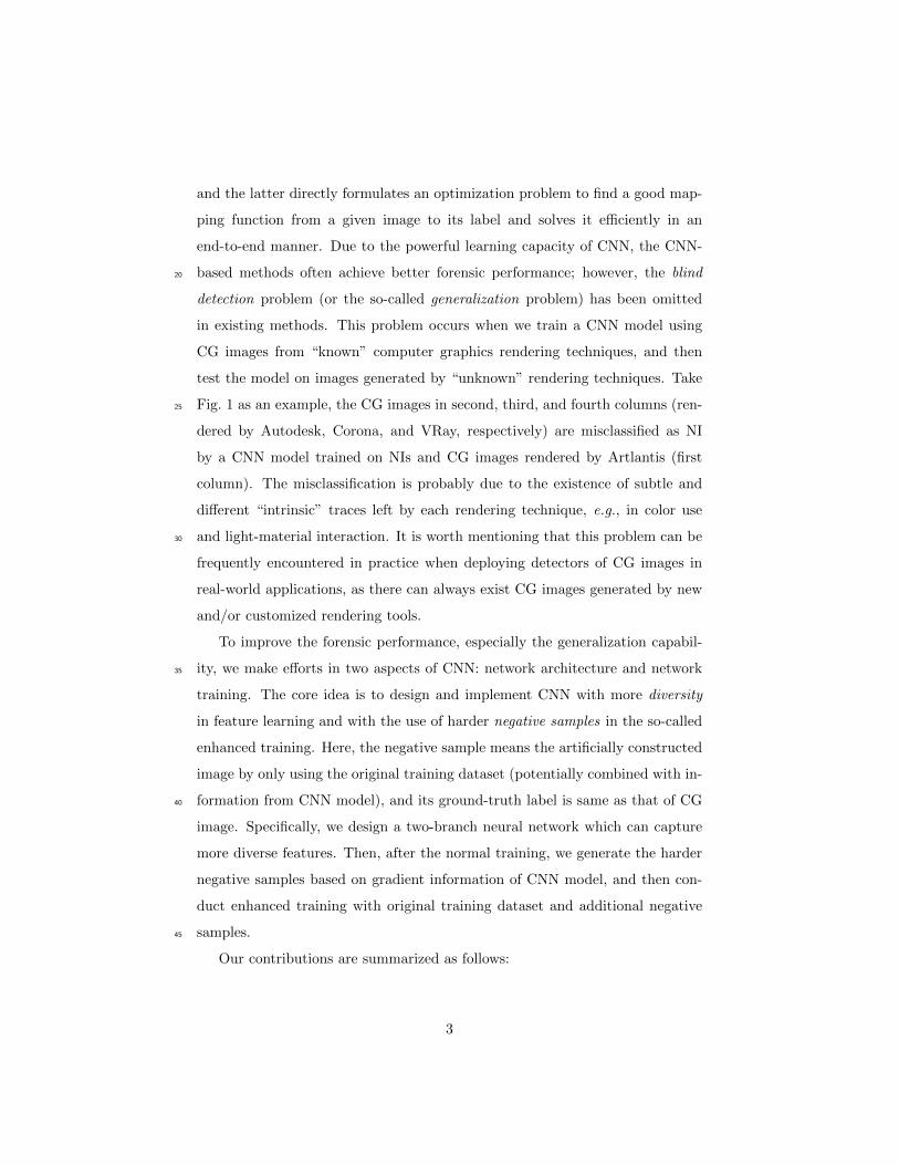
test the model on images generated by “unknown” rendering techniques. Take

Fig. 1 as an example, the CG images in second, third, and fourth columns (ren-25

dered by Autodesk, Corona, and VRay, respectively) are misclassified as NI

by a CNN model trained on NIs and CG images rendered by Artlantis (first

column). The misclassification is probably due to the existence of subtle and

different “intrinsic” traces left by each rendering technique, e.g., in color use

and light-material interaction. It is worth mentioning that this problem can be30

frequently encountered in practice when deploying detectors of CG images in

real-world applications, as there can always exist CG images generated by new

and/or customized rendering tools.

To improve the forensic performance, especially the generalization capabil-

ity, we make efforts in two aspects of CNN: network architecture and network35

training. The core idea is to design and implement CNN with more diversity

in feature learning and with the use of harder negative samples in the so-called

enhanced training. Here, the negative sample means the artificially constructed

image by only using the original training dataset (potentially combined with in-

formation from CNN model), and its ground-truth label is same as that of CG40

image. Specifically, we design a two-branch neural network which can capture

more diverse features. Then, after the normal training, we generate the harder

negative samples based on gradient information of CNN model, and then con-

duct enhanced training with original training dataset and additional negative

samples.45

Our contributions are summarized as follows:

3

• We first raise and study in the literature the generalization issue of the CG

image forensic problem. For the experimental study of this generalization

problem, we collect four computer graphics datasets which were generated

by four different rendering tools.50

• We design a new network which has better generalization. The beginning

part of the network has two branches with different initializations for the

first layer.

• We propose a novel and effective model-centric method to generate neg-

ative samples. Given a trained model and a CG image, we iteratively55

modify this image via gradient-based distortion to make the distorted

version close to the decision boundary of the CNN model. The gradient

can be easily computed using backpropagation.

The rest of this paper is organized as follows. Section 2 reviews related work.

Section 3 presents the datasets used for studying this generalization problem and60

for validating of our method. Section 4 discusses the motivation of our work,

and elaborates the details of the proposed method. Section 5 evaluates the

performance of our method. Section 6 draws the conclusions and discusses the

future working directions.

2. Related work65

2.1. Distinguishing between NIs and CG images

For the CG image forensic problem, there mainly exist two types of meth-

ods: hand-crafted-feature-based methods [6, 7, 8, 9, 10, 11, 12] and CNN-based

methods [13, 14, 15, 16, 17, 18, 19].

Hand-crafted-feature-based methods usually consist of two separate phases:70

(1) designing discriminative features; (2) training classifiers, e.g., support vec-

tor machine (SVM). The final detection performance heavily depends on the

discriminative capability of extracted features. Statistical methods are often

applied to construct features, such as the first-order and higher-order wavelet

4

statistics [7, 11], the statistical moments of wavelet characteristic function [8],75

the statistical property of local image edge patches [10], etc. The design of

features is more or less based on the prior knowledge of human beings, e.g., po-

tential differences between NI and CG images regarding the physical generation

process [6] and texture [12], and in practice these features often exhibit limited

forensic performance, especially on complex and challenging datasets [14].80

Inspired by the notable success of CNN in the field of computer vision and

pattern recognition, some recent works also applied CNN to solve the CG im-

age forensic problem [13, 14, 15, 16, 17, 18, 19]. Rahmouni et al. [13] explicitly

extracted low-order statistical information of convoluted image as discrimina-

tive features and trained a model to distinguish computer graphics from pho-85

tographic images. Quan et al. [14] proposed a CNN-based framework with

two cascaded convolutional layers in the beginning to identify NIs and CG im-

ages. They also tried to understand what the deep model has learned about

the differences between these two kinds of images by using a number of CNN

visualization tools. Yao et al. [15] proposed a method based on sensor pattern90

noise and CNN to solve this task. In their method, they used several high-pass

filters to enhance the residual signal as well as sensor pattern noise introduced

by the digital camera device. He et al. [16] combined CNN and recurrent neural

network (RNN) [20] to detect CG images. Nguyen et al. [17] used the capsule

network [21] for the CG image forensic problem. Bhalang Tarianga et al. [18]95

proposed an attention-based recurrent model to classify computer-generated

and natural images. Through exposing different characteristics between NIs

and CG images using the channel and pixel correlation information, Zhang et

al. [19] designed a hybrid-correlation-based CNN model.

While achieving decent classification accuracy on the detection of CG images,100

a very important issue, i.e., the generalization (or blind detection) problem, is

rarely studied by prior works. Very recently, Quan et al. [22] considered the

generalization problem in the task of colorized image detection, and proposed

negative-sample-based enhanced training to effectively improve the generaliza-

tion performance of CNN. In their work, they used linear interpolation of paired105

5

natural and colorized images to construct negative samples. Although this re-

quirement of paired images is not satisfied for the classification of NIs and CG

images, we extend this interpolation method in a straightforward way to the

unpaired setting and find that it can still improve the CNN’s generalization for

the CG image forensic problem. This data-centric method only uses training110

images and is “blind” to the CNN model; therefore, motivated by a poten-

tial performance boost, we propose a new and more effective method (so-called

model-centric method) by coupling the negative sample generation with the

gradient information of CNN loss function. This model-centric method borrows

idea from adversarial examples, and we briefly review this related topic in the115

next subsection.

2.2. Adversarial examples

In the following, we present some representative prior works on adversarial

examples which are closely related to our method. Readers could refer to recent

surveys [23, 24] for a comprehensive coverage of this rapidly evolving topic.120

Szegedy et al. [25] found an intriguing phenomenon: several high-performance

machine learning models, including advanced deep neural networks, are suscep-

tible to adversarial examples (or adversarial attacks). When applying a small

and imperceptible perturbation to a test sample, this perturbed version is very

likely to be misclassified by trained deep models. Goodfellow et al. [26] ex-125

plained that linearity in high-dimensional spaces is the primary cause of neural

networks’ vulnerability to adversarial perturbation. Based on this linear view,

they proposed the fast gradient sign method (FGSM) to generate adversarial

examples, where the required gradient can be computed efficiently using back-

propagation. This gradient-based method is the backbone of many subsequent130

construction methods of adversarial examples. FGSM is essentially a one-step

gradient-based method; therefore, a straightforward extension of this method is

to apply it in a multiple-step fashion with smaller step size (in extreme cases,

changing the value of each pixel only by 1 on each step) [27]. Tramer et al. [28]

proposed to prepend FGSM by a small random step, which is based on the sign135

6

of a Gaussian distribution.

In computer vision and machine learning, adversarial examples have been

used to improve the robustness of deep networks. There is less effort in the lit-

erature on using adversarial examples to improve network’s generalization. To

our knowledge, there is no such existing work in the image forensics community.140

In this paper, we propose a refined and appropriate method to generate adver-

sarial examples as negative samples (i.e., simulated proxy of “unknown” CG

images) for improving generalization. Specifically, our model-centric negative

sample generation method is based on a new iterative version of FGSM, i.e., we

randomly select certain percent of pixels to be changed by 1 for each step. The145

essential motivation of our method is to strictly control the strength of attack

(in other words and loosely speaking, the location of negative samples relative

to the decision boundary of CNN). Our method has different original intention

when compared to the conventional adversarial attacks in the field of machine

learning, where they prefer to maximally cross the decision boundary with as150

small as possible perturbation. Our method shares some similarities with the

iterative strategy of Tondi [29]; however, some differences exist: (1) [29] uses

adversarial examples to carry out attacks, while we use adversarial examples

to improve the generalization of CNN-based forensic detectors which is to our

knowledge new in the literature. (2) With some technical choices, our itera-155

tive version is more finely controlled in terms of the confidence level of negative

samples, which is important for the enhanced training.

3. Datasets

To study the generalization problem and validate our proposed method, we

collect four CG datasets1: Artlantis [2], Autodesk [3], Corona [4], and VRay [5].160

The CG images were downloaded from the websites of the four rendering soft-

ware tools. The collected CG images have high level of photorealism and are

1The datasets, either images or download links, will be made available upon request.

7

very close to real-world scenes. Some examples are shown in Fig. 1. The num-

ber of images of these four datasets are 1,620, 1,620, 1,593, and 1,579, respec-

tively. For each CG dataset, we randomly select 360 images as testing set, and165

the remaining images as training set (with the approximate ratio of 4:1). To

guarantee the diversity of NIs, we combine two datasets of RAISE [30] and VI-

SION [31] in our experiments. RAISE is a collection of 8,156 raw images that

were taken at very high resolution and we randomly select 4,700 images. In

order to simulate the real-world setting, we randomly resize and compress these170

raw images. For each raw image, we first resize with bicubic interpolation and

with the length of its shorter edge as an integer randomly sampled from the

set of {500, 750, 1000, 1500, 2000, 2500, 3000}. Then, we compress the resized

image with quality factor randomly sampled from the range of [70, 100]. VI-

SION is composed of images captured by 35 mobile devices where each device175

includes 100 natural images (in total 3,500 images). In addition, these natural

images were exchanged via the Facebook (high and low quality respectively) and

WhatsApp social media platforms, and thus each image has four versions (“nat”,

“natFBH”, “natFBL”, and “natWA” in [31]). Considering the same content of

these four versions, we randomly select one version for each image and obtain180

3,500 images. In the end, we have 8,200 NIs from RAISE and VISION.

In the following, we provide the details of datasets used in our experiments.

We randomly select 5,040 NIs and duplicate approximately 4 times of each CG

training set (5,040 CG images after duplication) to construct four final train-

ing datasets, corresponding respectively to the four rendering software tools185

(Artlantis, Autodesk, Corona, and VRay). From the remaining 3,160 NIs, we

respectively select 360 NIs for each CG dataset and combine corresponding test-

ing set (360 CG images) to construct four final testing datasets. The remaining

1,720 NIs constitute the so-called natural validation dataset, which is used for

the final CNN model selection in the stage of enhanced training (the details are190

described in Sec. 4.5).

8

4. Proposed method

4.1. Motivation

For the CG forensic problem, current CNN-based approaches can achieve

high classification accuracy. However, the performance of these forensic de-195

tectors often drops when testing the trained model on CG images generated

by “unknown” computer graphics rendering tools. To solve this generalization

problem, in this work, we consider two aspects of CNN: network architecture

and network training. Our network design is inspired by Quan et al.’ work [32]

about the impact of CNN’s first layer on forensic performance, where they pro-200

posed a simple criterion to combine the predictions of two independently trained

networks for obtaining the final result. In our work, we design and implement a

novel two-branch CNN model and apply different initialization strategy to the

first layer of these two branches. This network can be trained in the end-to-end

manner, and we expect to enrich the diversity of learned features through this205

ensemble-like design. For the network training, we adopt the enhanced train-

ing framework proposed in [22]. An important component of enhanced training

is the so-called negative samples, which are generated in [22] by linear inter-

polation of paired natural image and colorized image and which are deemed

to be more difficult to classify. In this work, we propose two types of genera-210

tion methods of negative samples (same label as CG images): (1) data-centric

method, which constructs negative sample via linear interpolation of unpaired

NI and CG image. (2) model-centric method, which generates negative sample

by modifying the CG image based on the gradient of CNN model.

4.2. Network architecture215

The standing point of our network design is to enrich the diversity of feature

learning. Inspired by the observation in [32] and ensemble learning, we design a

novel two-branch network to automatically and efficiently combine the kernels

initialized with SRM (Spatial Rich Model) filters [33] and Gaussian random

distribution in the beginning of network, and it can be trained in the standard220

9

FC

SRM

4096

k3n64 k3n64 k3n64

Input

FC(2)

Output

k5n30

SRM

SRM

RG

B

BN ReLUMax

Conv

BNConv

BN ReLU

Conv

BNConv

BN ReLU

Conv

Conv

k7n64s2 k5n48 k3n64 4096

L1 L2 L3 L4 L5 L6 L7 L8 L9 L10

B1

B2

Figure 2: Architecture of our network named ENet. The network input is a 233 × 233 RGB

image, and output is the class scores. For each convolutional layer, k is the kernel size, n is

the number of feature maps, and s is the stride. “FC(2)” stands for a fully-connected layer

with a 2-dimensional output of class scores. No padding exists in our network.

end-to-end way. This novel network is denoted by ENet (Ensemble Network),

and the corresponding network architecture is shown in Fig. 2. In practice, our

network takes the NcgNet proposed in [14] as backbone: the beginning part

(from L1 to L4 in Fig. 2) has a new two-branch design; starting from L5, the

network architecture is same as NcgNet. The input of ENet is an RGB image.225

After the first layer (so-called filter layer), we use three convolutional layers

without pooling operation (L2-4) to analyze the filtered signal. The analysis

results are concatenated (in the channel-wise manner) as the input of L5, and

three consecutive convolutional layers (L5-7) and two fully-connected layers (L8-

9) are applied to conduct high-level abstraction and reasoning. The last layer230

(L10) with softmax maps the high-level feature vector to the 2-dimensional class

scores (NI and CG). In total, ENet is a 10-layer network.

In our network, from L2 to L4, we do not use any pooling operation so as

to retain useful discriminative information, which also helps for improving the

diversity between the two branches. In the second branch (B2 in Fig. 2), the235

SRM means that the convolutional kernels are fixed as the thirty 5 × 5 SRM

residual filters borrowed from [33]. These three SRM blocks are applied to each

color channel of input image, i.e., R, G, and B, respectively. Then, all output

channels are directly concatenated together to form a ninety-channel input of

10

the second convolutional layer (L2). Except for the first layer (L1), each Conv240

is equipped with batch normalization (BN) layer. And we do not add activation

layer after L2 to preserve useful information as much as possible. Following [14],

all max-pooling layers have the same kernel size of 3× 3 and a stride of 2.

4.3. Data-centric method

This method constructs negative sample by linear interpolation, and the245

corresponding formulation is:

INS = α · INI + (1− α) · ICG, (1)

where INS is the negative sample, INI is the natural image, ICG is the computer-

generated image, and α ∈ {0.1, 0.2, 0.3, 0.4, · · · , 0.9, 0.99} is the interpolation

factor. For each factor, we randomly combine the NI and CG image of original

training dataset. To clearly illustrate this process with examples, we select four250

CG images, and then randomly select an NI for each CG image to generate the

negative sample via Eq. 1 with three different factors (α = 0.1, 0.5, 0.9). The

corresponding results are shown in Fig. 3. When α increases [from Fig. 3(c) to

Fig. 3(e)], the negative samples are progressively getting closer to the natural

images [Fig. 3(b)]. In addition, we allow the use of larger interpolation factor255

than the work in [22], i.e., α > 0.4, mainly due to the “blind” nature of this

method, i.e., it is blind to the decision boundary of trained CNN model.

4.4. Model-centric method

This method is related to the gradient-sign-based adversarial sample gen-

eration. In this subsection, we first recall the formulation of FGSM [26] and260

its iterative variant [27]. Then, we describe our iterative masked gradient sign

method (IMGSM) for constructing negative sample.

Let x be the original (or clean) image, x the perturbed version of x with

expected target t, M a deep model and JM(x, t) the loss function (e.g., cross-

entropy loss) used to train the original model M. The formulation of FGSM is265

x = x− εsign(OxJM(x, t)), (2)

11

(a)

(b)

(c)

(d)

(e)

Figure 3: Examples of data-centric method. From top to bottom: (a) four CG images rendered

by Corona [4]; (b) randomly selected NI for each CG image; (c), (d), and (e): the negative

samples generated by Eq. 1 with CG image and NI in (a) and (b) of the same column, where

the interpolation factor α is 0.1, 0.5, and 0.9, respectively. We calculate the PSNR (peak

signal-to-noise ratio) for the negative samples [(c), (d), and (e)], with the CG image [(a)] as

the reference. PSNR values (in dB) from left to right: (c) 28.12, 28.42, 28.09, and 27.32; (d)

14.24, 14.44, 14.31, and 13.12; (e) 9.14, 9.33, 9.20, and 8.02.

12

where hyper-parameter ε controls the magnitude of the perturbation.

An iterative variant of FGSM is

xk+1 = Clipx,ε{xk − βsign(OxJM(xk, t))}, (3)

where Clipx,ε{x′} is the operation which projects the image x′ into the L∞

ε-neighbourhood of the source image x [27]. Usually, the value of β depends on270

the data type of image pixel (integer or float) and is set following the minimal

distortion, i.e., changing the pixel value only by 1 for each modification.

Our goal is to modify a CG image x and output a harder negative sample

x with predicted probability p as NI under original trained model. x plays

the role of simulated proxy of “unknown” CG image that may be encountered275

during testing. To exactly control the predicted probability of negative sample,

we introduce the iterative masked gradient sign method (IMGSM). Compared

with Eq. 3, our formulation of IMGSM has two differences: (1) we have no clip

operation because we mainly consider the attack confidence of negative sample

(i.e., the probability p) and do not need to strictly limit the magnitude of the280

perturbation. (2) we introduce the random-mask-based strategy to perturb the

input image for each modification so that we can exactly control the attack con-

fidence of negative sample, e.g., falling into a certain interval. The formulation

is

xk+1 = xk − βmλ � sign(OxJM(xk, t)), (4)

where � is the element-wise product operation and mλ is the binary mask whose285

elements are randomly set as zeroes with probability λ. Note that x, O, and

mλ have the same shape. In our experiment, the 8-bit integer pixel is scaled to

float in [−1, 1], therefore, we set β = 2/255 to guarantee the minimal distortion.

In other words, after transforming back to the integer pixel value, ±β on float

means adding or subtracting by 1.290

Algorithm 1 illustrates the process of model-centric negative sample gen-

eration. To constrain the predicted confidence of generated negative sample

belonging to a certain interval [pmin,pmax], we introduce adaptive strategy to

adjust the mask probability λ shown in line 14-18 of Algorithm 1. Starting

13

Algorithm 1 Iterative masked gradient sign method

Input: trained model M, x, attack confidence interval [pmin,pmax], the max-

imal iterations K = 200, the initial mask probability λ0 = 0.96.

Output: negative sample x.

Initialization: current mask probability λ = λ0, p is set as the predicted

confidence of x as NI.

1: while p < pmin and λ <= 0.998 do

2: set x0 = x, xcand = x.

3: for k = 0 to K − 1 do

4: compute OxJM(xk, t) using backpropagation.

5: compute xk+1 via Eq. 4.

6: compute current attack confidence p of xk+1.

7: if p > pmax then

8: break.

9: else

10: set xcand = xk+1.

11: end if

12: end for

13: set x = xcand, and compute the attack confidence p of x.

14: if λ < 0.99 then

15: λ = λ+ 0.01.

16: else

17: λ = λ+ 0.002.

18: end if

19: end while

14

0.96 0.97 0.98 0.99 1Mask probability

0

200

400

600

800

1000

1200

1400

#Num

(a)

0 10 20 30 40 50 600

200

400

600

800

#Num

(b)

0 0.1 0.2 0.3 0.4 0.5 0.6 0.7 0.8 0.9 10

1000

2000

3000

4000

#Num

(c)

0 0.1 0.2 0.3 0.4 0.5 0.6 0.7 0.8 0.9 10

50

100

150

200

250

300

#Num

(d)

Figure 4: The statistics of model-centric negative sample generation: (a) mask probability λ,

(b) iterations k, (c) the predicted probability p of original CG images, and (d) the predicted

probability p of corresponding negative samples.

from a minimal value of λ which experimentally leads to large distortion (thus295

large jump of p) for each modification while iterating on k in line 3, the mask

probability progressively increases when the predicted probability of generated

negative sample cannot fall into the required interval. A mask with higher value

of λ leads to milder increase of p in each iteration, with more chance to meet

the constraint of required interval for p. In our experiment, we choose the300

confidence interval of generated negative sample as [0.3, 0.5], which means the

negative sample is close to original classification boundary and in the side of

CG image.

To clearly illustrate the process of model-centeric negative sample generation

15

Figure 5: Four groups of CG sample (top row) and corresponding negative sample (bottom

row) based on model-centric method. We calculate the PSNR for the negative sample, with

the CG sample as the reference. PSNR values (in dB) from left to right: 56.32, 58.92, 56.63,

and 56.25, respectively.

with an example, we train the ENet on Corona, and then generate the nega-305

tive samples of CG images in training dataset (in total, 5040 images). Fig. 4

shows the histogram of mask probability λ (a), iterations k (b), and predicted

probability p of original CG images (c) and corresponding negative samples (d).

Given a CG image, it is difficult to derive an algorithm which can theoretically

guarantee that the predicted probability p of negative sample strictly falls into310

the expected interval (i.e., [0.3, 0.5] in our experiment). In practice, by using

our adaptive mask strategy, we observe that experimentally almost all negative

samples can successfully fall into this interval, like Fig. 4(d), where only two

samples are not in [0.3, 0.5]. This is because the two original CG images have

p value larger than 0.5, i.e., 0.76 and 0.64.315

In addition, Fig. 5 shows four groups of negative samples (bottom row)

based on model-centric method and corresponding CG images (top row). From

left to right: for CG sample, p = 2.40e-5, 4.92e-3, 1.95e-4, 2.01e-4; for negative

samples, p = 0.32, 0.38, 0.48, 0.35. Comparing the two rows, we can find that

the CG images and the corresponding negative samples are visually almost the320

16

same (see PSNR values in the caption of Fig. 5). Furthermore, compared with

the PSNR values reported in the caption of Fig. 3, those of Fig. 5 are obviously

larger, which means that the perturbation introduced by model-centric method

is much smaller. We also analyze the min/max perturbation for CG images in

Fig. 5, i.e., the minimal/maximal perturbation value for pixels within an image.325

The min/max perturbations are from left to right: −3/3, −3/2, −3/3, and−4/3,

respectively (pixel values are in the range of 0 to 255). These results demonstrate

that when generating negative samples, gradient-based perturbation modifies

very slightly the pixels of CG images in an almost imperceptible way.

4.5. Network training330

In our work, a complete network training includes two stages: normal train-

ing and enhanced training. The CNN model first conducts normal training from

scratch with the original training dataset D, i.e., NIs and CG images generated

by “known” rendering tools. After the model converges, we continue to train

the model with enhanced training based on negative sample insertion. This335

enhanced training is an iterative process, and the main pipeline is described as

follows.

• We construct negative samples using Eq. 1 or Algorithm 1, and insert

them into D.

• We update the parameters of M using D. Starting from the second half340

of training process, we compute the error rate r on the so-called natural

validation dataset V and also mark the model as candidate model if its

r is less than θ (a threshold that determines the accepted degree of final

classification accuracy on NIs; in our experiment, we set θ = 4%).

• The above two steps interleave until reaching the stop condition. If the345

error rates on V starting from the second half of training process are all

larger than θ, we stop the iteration process; otherwise, we stop when the

number of iterations reaches maximal value Z: for data-centric method,

17

Z = 10 (α can take 10 values, see in Sec. 4.3); for model-centric method,

Z = 20.350

• From all candidate models, we select the final model which has the maxi-

mal r.

5. Experimental results

5.1. Implementation details

All the experiments are implemented with PyTorch. The GPU version is355

GeForce R© GTX 1080Ti of NVIDIA R© corporation. In this work, we consider

two recent state-of-the-art CNN models of YaoNet [15] and NcgNet [14]. In [15],

the images are first converted to grayscale and then fed into YaoNet to reduce

the computational complexity. For convenience and fair comparisons, we di-

rectly use RGB images as the input of YaoNet and this variant achieves better360

performance compared with grayscale input. Following [14], all images in our

experiments are resized using bicubic interpolation so that the shorter edge of

each resized image has 512 pixels, and for each image, we rescale its pixel values

to [−1, 1]. The input size of network is 233 × 233. Stochastic gradient descent

(SGD) with a minibatch of 32 is used to train ENet. For SGD optimizer, the365

momentum is 0.9 and the weight decay is 1e-4. The initial learning rate is 1e-3.

For the normal training (only using original training dataset) of ENet, we di-

vide the learning rate by 10 every 100 epochs, and the training procedure stops

after 300 epochs. For the normal training of YaoNet and NcgNet, we follow the

same learning rate schedule as described respectively in [15] and [14]. In the370

stage of enhanced training of these three networks, we adopt the same strategy

about learning rate: the learning rate is continued to be divided by 10 every 15

epochs (one insertion) and fixed after 4 iterations of negative sample insertion to

avoid learning rate becoming too small. Following [14], we adopt the standard

10-crop testing [34]: given a testing sample, the network extracts five patches375

of 233× 233 pixels (the center and four corner patches), flips these five patches

18

Table 1: The classification performance (HTER, in %, lower is better) of different network

architectures. “NcgNet Comb” is the combination result of predictions of “NcgNet” and

“NcgNet SRM” according to the combination criterion used by [32]. For the sake of clarity,

the results of generalization performance on “unknown” rendering engines are presented in

italics.

Network Autodesk Artlantis Corona VRay

YaoNet 4.61 28.14 15.00 21.17

NcgNet 2.84 16.61 12.78 16.58

NcgNet SRM 2.42 17.97 8.97 16.09

NcgNet Comb 2.16 13.14 7.75 12.61

ENet 1.56 10.39 7.67 13.39

in the left-right direction (i.e., horizontal reflection), and then averages the pre-

dictions of total 10 patches as the final result. We employ the half total error

rate (HTER) to evaluate the detection performance. The HTER is defined as

the average of misclassification rates (in %) of NIs and CG images, here same380

as the overall error rate on balanced testing datasets. In this work, all reported

results are the average of 5 runs.

5.2. Validation of our proposed network

We validate our network architecture design of ENet in terms of the conven-

tional classification performance and the generalization capability. All the net-385

works are trained on Autodesk and tested on Artlantis, Corona, and VRay. The

corresponding results are reported in Table 1. Compared with YaoNet, NcgNet

and NcgNet SRM, ENet demonstrates better performance for both “known” and

“unknown” rendering engines. Here, the NcgNet SRM is the variant of NcgNet

where the first layer of NcgNet is replaced with three SRM blocks like the first390

layer of B2 in Fig. 2. In addition, although NcgNet Comb and ENet have com-

parable results, the former needs to train two models separately, i.e., which

inevitably and approximately doubles the number of parameters and training

time.

Next, we evaluate the performance of four variants of our proposed ENet,395

19

Table 2: The classification performance (HTER, in %, lower is better) of our proposed ENet

and its four variants. All networks are trained on Autodesk. The results of generalization

performance on “unknown” rendering engines are presented in italics.

Network Autodesk Artlantis Corona VRay

ENet d 2.00 15.06 10.25 16.11

ENet SRM 2.00 11.19 7.30 13.44

ENet d half 1.72 12.53 8.44 13.44

ENet rand 2.28 15.97 10.33 16.89

ENet 1.56 10.39 7.67 13.39

i.e., ENet d, ENet SRM, ENet d half, and ENet rand. We remove the B2 of

ENet (the blue dotted rectangle in Fig. 2) and double the number of feature

maps of L3 and L4 to obtain ENet d. Similarly, we remove the B1 of ENet

(the red dotted rectangle in Fig. 2) and also double the number of feature maps

of L3 and L4 to obtain ENet SRM. For ENet d half, we combine the three400

SRM blocks with the first layer of ENet d, i.e., concatenating the outputs of

these three SRM blocks with the output of first layer of ENet d to form a 120-

channel input of the L2 of ENet d. In addition, we use the Gaussian random

distribution to initialize the first layer of B2 of ENet and make the corresponding

ninety kernels trainable, and this replaces the B2’s original setting of using fixed405

SRM filters. The corresponding model is denoted by ENet rand. Note that, the

number of parameters of these four variants are slightly larger than that of ENet.

Among these five networks, the ENet achieves better overall performance (see

Table 2). We find that ENet outperforms ENet rand (comparing the row of

“ENet rand” and “ENet”). This demonstrates that our ensemble-like design,410

with different intializations at the first layer of the two branches, can improve

the performance of network, especially generalization. It can also be observed

that ENet SRM and ENet d half have satisfying performance and that the ENet

can further decrease the conventional classification error rate meanwhile slightly

improving the overall generalization. Our conjecture is that convolutional layers415

without pooling operation in the front part of the two-branch structured ENet

20

(a) (b)

(c) (d)

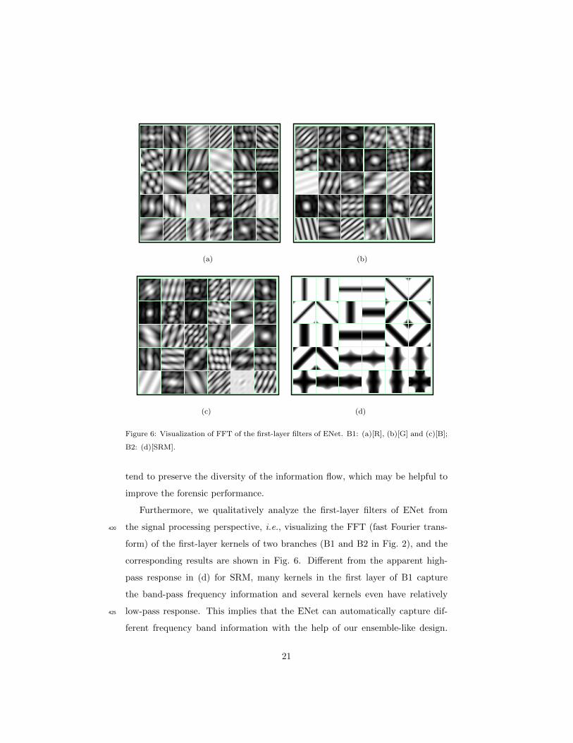
Figure 6: Visualization of FFT of the first-layer filters of ENet. B1: (a)[R], (b)[G] and (c)[B];

B2: (d)[SRM].

tend to preserve the diversity of the information flow, which may be helpful to

improve the forensic performance.

Furthermore, we qualitatively analyze the first-layer filters of ENet from

the signal processing perspective, i.e., visualizing the FFT (fast Fourier trans-420

form) of the first-layer kernels of two branches (B1 and B2 in Fig. 2), and the

corresponding results are shown in Fig. 6. Different from the apparent high-

pass response in (d) for SRM, many kernels in the first layer of B1 capture

the band-pass frequency information and several kernels even have relatively

low-pass response. This implies that the ENet can automatically capture dif-425

ferent frequency band information with the help of our ensemble-like design.

21

This is beneficial to enrich the extracted features and to improve the detection

performance.

5.3. Effect of enhanced training

In this work, we introduced two types of negative sample generation: data-430

centric method and model-centric method. To verify the effectiveness of these

two methods for generalization improvement, we conduct extensive experiments

with three CNN models on four datasets. We report in Table 3, 4, 5, and 6

the performance before (the column of “NT”) and after (the columns of “ET-

I” and “ET-G”) enhanced training of YaoNet, NcgNet, and ENet, when they435

are trained on Artlantis, Autodesk, Corona, and VRay, respectively. For each

table, starting from the second column, each consecutive three columns form

a group, in total four groups. The first group (e.g., “Artlantis” in Table 3)

is the conventional classification error rate, and the remaining three groups

(e.g., “Autodesk”, “Corona”, and “VRay” in Table 3) are the generalization440

performance.

From Table 3-6, we find that enhanced training with negative sample in-

sertion based on data-centric and model-centric methods usually leads to slight

increase of conventional classification error rate; however, the generalization of

the three networks can be apparently and consistently improved by these two445

methods (except for one case in Table 5, when we trained YaoNet on Corona

with data-centric method and tested on VRay, with a small increase of HTER

by 1.39% from 9.14% to 10.53%, but model-centric method can decrease it to

7.19%). As an example of performance improvement, when we trained ENet on

Artlantis with enhanced training based on model-centric method (comparing the450

columns of “NT” and “ET-G” of the last row in Table 3), the conventional clas-

sification accuracy decreases by 1.44%, whereas the generalization is improved

by 5.75%(Autodesk), 7.30%(Corona), and 6.36%(VRay), respectively. Further-

more, in Table 3-6, the HTER value of ENet is always the lowest among three

networks except for one case (3.08% in Table 4, i.e., training on Autodesk and455

testing on Autodesk with data-centric method). This illustrates our proposed

22

Table 3: Performance (HTER, in %, lower is better) of three networks when trained on Art-

lantis. “NT” stands for normal training; “ET-I” and “ET-G” stands for enhanced training

with negative samples produced by unpaired linear interpolation and gradient-based distor-

tion, respectively; The generalization performance results on “unknown” rendering engines

are in italics (same for Table 4, 5, and 6).

NetworkArtlantis Autodesk Corona VRay

NT ET-I ET-G NT ET-I ET-G NT ET-I ET-G NT ET-I ET-G

YaoNet 3.86 5.17 3.94 20.31 12.61 12.64 18.17 14.14 13.72 15.11 13.42 12.47

NcgNet 3.17 3.47 3.61 12.69 8.47 8.17 16.00 11.72 11.22 12.58 10.78 9.58

ENet 1.31 2.31 2.75 10.06 5.09 4.31 14.58 8.15 7.28 11.86 7.22 5.50

Table 4: Performance (HTER, in %, lower is better) of three networks when trained on

Autodesk.

NetworkAutodesk Artlantis Corona VRay

NT ET-I ET-G NT ET-I ET-G NT ET-I ET-G NT ET-I ET-G

YaoNet 4.61 3.86 2.72 28.14 22.50 16.84 15.00 11.31 8.00 21.17 16.00 12.97

NcgNet 2.84 2.87 2.67 16.61 11.48 11.03 12.78 9.50 9.06 16.58 12.32 12.64

ENet 1.56 3.08 2.39 10.39 5.64 5.58 7.67 5.39 4.86 13.39 7.47 8.22

Table 5: Performance (HTER, in %, lower is better) of three networks when trained on Corona.

NetworkCorona Artlantis Autodesk VRay

NT ET-I ET-G NT ET-I ET-G NT ET-I ET-G NT ET-I ET-G

YaoNet 3.79 3.79 3.28 19.53 17.17 11.33 10.87 10.50 8.42 9.14 10.53 7.19

NcgNet 2.73 3.06 2.81 21.74 15.05 13.69 9.56 7.25 7.67 8.08 6.11 5.75

ENet 1.50 2.72 2.14 16.08 7.61 6.39 7.92 6.83 7.03 7.78 4.36 4.39

Table 6: Performance (HTER, in %, lower is better) of three networks when trained on VRay.

NetworkVRay Artlantis Autodesk Corona

NT ET-I ET-G NT ET-I ET-G NT ET-I ET-G NT ET-I ET-G

YaoNet 4.28 4.22 3.64 16.77 15.75 11.64 15.30 11.89 9.64 9.05 7.47 6.33

NcgNet 3.20 3.53 2.84 14.06 10.19 8.97 15.00 8.86 8.53 5.53 5.17 5.33

ENet 1.25 2.22 1.72 11.58 6.94 5.39 9.97 5.97 6.08 4.53 4.31 3.17

ENet has the superior performance.

We also compare the performance of data-centric and model-centric based

enhanced training with that of “mixup” [35]. “mixup” is a learning principle to

23

Table 7: Performance (HTER, in %, lower is better) of ENet. Each row stands for the

training dataset. Starting from the second column, each consecutive four columns form a

group, and each group stands for the testing dataset. “NT” stands for normal training; “ET-

I” and “ET-G” stand for enhanced training with negative samples produced by unpaired

linear interpolation (data-centric) and gradient-based distortion (model-centric), respectively;

“MU” stands for “mixup” [35]. The generalization performance results are in italics.

DatasetArtlantis Autodesk Corona VRay

NT ET-I ET-G MU NT ET-I ET-G MU NT ET-I ET-G MU NT ET-I ET-G MU

Artlantis 1.31 2.31 2.75 1.75 10.06 5.09 4.31 11.95 14.58 8.15 7.28 16.03 11.86 7.22 5.50 11.86

Autodesk 10.39 5.64 5.58 13.30 1.56 3.08 2.39 1.70 7.67 5.39 4.86 9.44 13.39 7.47 8.22 14.44

Corona 16.08 7.61 6.39 14.67 7.92 6.83 7.03 6.97 1.50 2.72 2.14 1.31 7.78 4.36 4.39 6.06

VRay 11.58 6.94 5.39 9.22 9.97 5.97 6.08 9.72 4.53 4.31 3.17 4.33 1.25 2.22 1.72 1.19

regularize the neural network and encourage the trained model to behave lin-460

early in-between training examples. We train the ENet with “mixup” and set its

hyperparameter α = 0.4 as recommended in [35]. All the results are reported

in Table 7. Comparing the columns of “MU” with “ET-I” and “ET-G”, we

find that data-centric and model-centric based enhanced training significantly

outperforms “mixup”. Furthermore, the generalization performance of “mixup”465

sometimes is worse than that of normal training (without “mixup”), e.g., train-

ing on Autodesk and testing on Artlantis (10.39% vs. 13.30%). A possible rea-

son is that “mixup” is essentially a form of data augmentation that implicitly

affects the generalization of trained CNN model (in fact, this sometimes cannot

guarantee the improvement of generalization as reported in Table 7 and men-470

tioned above), whereas data-centric and model-centric based enhanced training

can explicitly change the decision boundary and then improve the generalization

of CNN-based detectors.

As shown above with experimental results, model-centric negative sample

insertion usually achieves better performance in terms of conventional classifi-475

cation accuracy and generalization capability, especially for YaoNet, when com-

pared with data-centric method. The reason is that model-centric method can

more exactly control the location of negative samples relative to the decision

boundary in the feature space of CNN, and thus more effectively improve the

generalization with relatively small decrease of the classification accuracy on480

24

(a) (b)

Figure 7: The deep feature visualization of YaoNet with t-SNE [36]. “C” means computer-

generated images and “N” means natural images. “C-Auto” means the CG images rendered

by Autodesk and “C-NS” means the negative samples generated by data-centric method (a)

and model-centric method (b). “Y-pred” means that the predicted label of CNN is Y. NIs

and CG images are randomly selected from training dataset for visualization.

NIs. To clearly illustrate the location of negative samples generated by data-

centric and model-centric methods in the feature space, we train YaoNet on

NIs and CG images rendered by Autodesk. We visualize the deep features of

negative samples in the last insertion of enhanced training with t-SNE [36], and

results are shown in Fig. 7. In Fig. 7(a), many negative samples are mixed with485

point cloud of NIs and predicted as NI (blue diamonds with red +) because

the linear interpolation is conducted in the image space and “blind” to CNN.

On the contrary, all negative samples of model-centric method in Fig. 7(b) are

predicted as CG (blue diamonds with blue +) and almost located in the middle

of point clouds of NIs and CG images.490

5.4. Discussion

In our study, we first observe a new problem regarding the generalization

performance of CG forensics, then propose a new method to cope with this

challenging problem, and finally validate the proposed method with extensive

experiments. New understanding we get from this study is mainly the following:495

when we roughly know that a class may have a relatively large distribution

25

change during testing, we can use our method to generate proxy samples of the

“unknown” distributions by only using available training data; the enhanced

training with such samples is effective to improve generalization. This is valid

for the 12 (4*3) tested cases. Our work is a small step towards the ultimate500

goal of fully understanding CNN’s generalization. We have also tried to gain

new understanding with FFT of first-layer filters and t-SNE visualization, which

may provide useful insights to colleagues.

6. Conclusion

In this work, we studied and solved the challenging blind detection problem505

of CG image forensics. To facilitate this study, we collected four CG datasets

with high level of photorealism. We designed and implemented a novel two-

branch network with different initializations in their respective first layer to

extract more diverse features, and this network has good generalization per-

formance. In the meanwhile, we also introduced the data-centric and model-510

centric negative sample generation used for conducting enhanced training. This

can further improve the generalization performance of CNN-based detectors.

More information and materials, including the source code, are available at

https://github.com/weizequan/CGDetection.

For this new and challenging CG forensic problem, our method does not of-515

fer a rigorous framework/formulation, which can be considered as a limitation.

However, this might also be an advantage: e.g., we avoid implicit restrictions

due to mathematical modeling, such as specific hypothesized parameterization

of the distributions of “unknown” CG images. Further, our approach does not

use any sample or prior knowledge of new distributions, which is usually neces-520

sary for a rigorous formulation (e.g., in many domain adaptation algorithms).

This makes our method simple, flexible and generic because our assumption

is very weak and everything is done “off-line” at the training side. In the fu-

ture, we plan to study the generalization improvement with a suitable rigorous

formulation. Our proposed method and such a future method are not contradic-525

26

tory, and can even complement each other, e.g., our “off-line” method applied

first, before an “on-line” continual learning method. Last but not least, our

study implies that in order to improve generalization it is beneficial to learn

diverse features and to learn from harder artificial samples. We would like to

test this idea in other research problems and in the meanwhile explore other530

approaches to understanding and enhancing the generalization of CNN-based

forensic detectors.

Acknowledgment

This work was funded in part by the National Natural Science Founda-

tion of China (61772523 and 61620106003), the National Key R&D Program of535

China (2019YFB2204104), the Beijing Natural Science Foundation (L182059),

and the French National Agency for Research through PERSYVAL-lab under

Grant ANR-11-LABX-0025-01 and through DEFALS under Grant ANR-16-

DEFA-0003. W. Quan acknowledges the support from the UCAS Joint PhD

Training Program. We thank Dr. D.-T. Dang-Nguyen and Dr. D. Shullani for540

kindly sharing the RAISE [30] and VISION [31] dataset respectively.

References

[1] T. Yamaguchi, T. Yatagawa, Y. Tokuyoshi, S. Morishima, Real-time ren-

dering of layered materials with anisotropic normal distributions, Compu-

tational Visual Media 6 (1) (2020) 29–36.545

[2] Artlantis gallery, https://atl.artlantis.com/en/gallery/, (visited on

2020-03-11).

[3] Autodesk A360 rendering gallery, https://gallery.autodesk.com/

a360rendering/, (visited on 2020-03-11).

[4] Corona renderer gallery, https://corona-renderer.com/gallery, (vis-550

ited on 2020-03-11).

27

[5] Chaosgroup gallery, https://www.chaosgroup.com/gallery; Learn V-

Ray gallery, https://www.learnvray.com/fotogallery/, (visited on

2020-03-11).

[6] T.-T. Ng, S.-F. Chang, J. Hsu, L. Xie, M.-P. Tsui, Physics-motivated fea-555

tures for distinguishing photographic images and computer graphics, in:

Proceedings of the ACM International Conference on Multimedia, 2005,

pp. 239–248.

[7] S. Lyu, H. Farid, How realistic is photorealistic?, IEEE Transactions on

Signal Processing 53 (2) (2005) 845–850.560

[8] W. Chen, Y. Q. Shi, G. Xuan, Identifying computer graphics using HSV

color model and statistical moments of characteristic functions, in: Pro-

ceedings of the IEEE International Conference on Multimedia & Expo,

2007, pp. 1123–1126.

[9] A. C. Gallagher, T. Chen, Image authentication by detecting traces of565

demosaicing, in: Proceedings of the IEEE Conference on Computer Vision

and Pattern Recognition, 2008, pp. 1–8.

[10] R. Zhang, R.-D. Wang, T.-T. Ng, Distinguishing photographic images and

photorealistic computer graphics using visual vocabulary on local image

edges, in: Proceedings of the International Workshop on Digital-Forensics570

and Watermarking, 2012, pp. 292–305.

[11] J. Wang, T. Li, Y.-Q. Shi, S. Lian, J. Ye, Forensics feature analysis in

quaternion wavelet domain for distinguishing photographic images and

computer graphics, Multimedia Tools and Applications 76 (22) (2017)

23721–23737.575

[12] F. Peng, D.-L. Zhou, M. Long, X.-M. Sun, Discrimination of natural im-

ages and computer generated graphics based on multi-fractal and regression

analysis, AEU - International Journal of Electronics and Communications

71 (2017) 72–81.

28

[13] N. Rahmouni, V. Nozick, J. Yamagishi, I. Echizen, Distinguishing com-580

puter graphics from natural images using convolution neural networks, in:

Proceedings of the IEEE International Workshop on Information Forensics

and Security, 2017, pp. 1–6.

[14] W. Quan, K. Wang, D.-M. Yan, X. Zhang, Distinguishing between natural

and computer-generated images using convolutional neural networks, IEEE585

Transactions on Information Forensics and Security 13 (11) (2018) 2772–

2787.

[15] Y. Yao, W. Hu, W. Zhang, T. Wu, Y. Q. Shi, Distinguishing computer-

generated graphics from natural images based on sensor pattern noise and

deep learning, Sensors 18 (4).590

[16] P. He, X. Jiang, T. Sun, H. Li, Computer graphics identification combin-

ing convolutional and recurrent neural networks, IEEE Signal Processing

Letters 25 (9) (2018) 1369–1373.

[17] H. H. Nguyen, J. Yamagishi, I. Echizen, Capsule-forensics: Using capsule

networks to detect forged images and videos, in: Proceedings of the IEEE595

International Conference on Acoustics, Speech and Signal Processing, 2019,

pp. 2307–2311.

[18] D. Bhalang Tarianga, P. Senguptab, A. Roy, R. Subhra Chakraborty,

R. Naskar, Classification of computer generated and natural images based

on efficient deep convolutional recurrent attention model, in: Proceedings of600

the IEEE Conference on Computer Vision and Pattern Recognition Work-

shops, 2019, pp. 146–152.

[19] R. Zhang, W. Quan, L. Fan, L. Hu, D.-M. Yan, Distinguishing computer-

generated images from natural images using channel and pixel correlation,

Journal of Computer Science and Technology 35 (3) (2020) 592–602.605

[20] B. Shuai, Z. Zuo, B. Wang, G. Wang, Dag-recurrent neural networks for

29

scene labeling, in: Proceedings of the IEEE Conference on Computer Vision

and Pattern Recognition, 2016, pp. 3620–3629.

[21] S. Sabour, N. Frosst, G. E. Hinton, Dynamic routing between capsules, in:

Proceedings of the Advances in Neural Information Processing Systems,610

2017, pp. 3856–3866.

[22] W. Quan, K. Wang, D.-M. Yan, D. Pellerin, X. Zhang, Improving the gen-

eralization of colorized image detection with enhanced training of CNN, in:

Proceedings of the International Symposium on Image and Signal Process-

ing and Analysis, 2019, pp. 246–252.615

[23] N. Akhtar, A. Mian, Threat of adversarial attacks on deep learning in

computer vision: A survey, IEEE Access 6 (2018) 14410–14430.

[24] X. Yuan, P. He, Q. Zhu, X. Li, Adversarial examples: Attacks and defenses

for deep learning, IEEE Transactions on Neural Networks and Learning

Systems 30 (9) (2019) 2805–2824.620

[25] C. Szegedy, W. Zaremba, I. Sutskever, J. Bruna, D. Erhan, I. Goodfel-

low, R. Fergus, Intriguing properties of neural networks, in: International

Conference on Learning Representations, 2014.

[26] I. Goodfellow, J. Shlens, C. Szegedy, Explaining and harnessing adversarial

examples, in: International Conference on Learning Representations, 2015.625

[27] A. Kurakin, I. J. Goodfellow, S. Bengio, Adversarial examples in the phys-

ical world, CoRR abs/1607.02533.

[28] F. Tramer, A. Kurakin, N. Papernot, I. Goodfellow, D. Boneh, P. Mc-

Daniel, Ensemble adversarial training: Attacks and defenses, in: Interna-

tional Conference on Learning Representations, 2018.630

[29] B. Tondi, Pixel-domain adversarial examples against CNN-based manipu-

lation detectors, Electronics Letters 54 (21) (2018) 1220–1222.

30

[30] D.-T. Dang-Nguyen, C. Pasquini, V. Conotter, G. Boato, RAISE: A raw

images dataset for digital image forensics, in: Proceedings of the ACM

Multimedia Systems Conference, 2015, pp. 219–224.635

[31] D. Shullani, M. Fontani, M. Iuliani, O. A. Shaya, A. Piva, VISION: a

video and image dataset for source identification, EURASIP Journal on

Information Security 2017 (1) (2017) 15.

[32] W. Quan, K. Wang, D.-M. Yan, D. Pellerin, X. Zhang, Impact of

data preparation and CNN’s first layer on performance of image foren-640

sics: A case study of detecting colorized images, in: Proceedings of the

IEEE/WIC/ACM International Conference on Web Intelligence – Com-

panion Volume, 2019, pp. 127–131.

[33] J. Fridrich, J. Kodovsky, Rich models for steganalysis of digital images,

IEEE Transactions on Information Forensics and Security 7 (3) (2012) 868–645

882.

[34] A. Krizhevsky, I. Sutskever, G. E. Hinton, ImageNet classification with

deep convolutional neural networks, in: Proceedings of the Advances in

Neural Information Processing Systems, 2012, pp. 1097–1105.

[35] H. Zhang, M. Cisse, Y. N. Dauphin, D. Lopez-Paz, mixup: Beyond empir-650

ical risk minimization, in: Proceedings of the International Conference on

Learning Representations, 2018.

[36] L. van der Maaten, G. E. Hinton, Visualizing high-dimensional data using

t-SNE, Journal of Machine Learning Research 9 (2008) 2579–2605.

31