leaf thickness and electrical capacitance as …
TRANSCRIPT

The Pennsylvania State University
The Graduate School
College of Agricultural Sciences
LEAF THICKNESS AND ELECTRICAL CAPACITANCE AS MEASURES
OF PLANT WATER STATUS
A Dissertation in
Agronomy
by
Sayed Amin Afzal
© 2017 Sayed Amin Afzal
Submitted in Partial Fulfillment
of the Requirements
for the Degree of
Doctor of Philosophy
May 2017

The dissertation of Sayed Amin Afzal was reviewed and approved* by the following:
Sjoerd Willem Duiker
Associate Professor of Soil Management
and Applied Soil Physics
Dissertation Co-Adviser
Co-Chair of Committee
John E. Watson
Professor of Soil Science/Soil Physics
Dissertation Co-Adviser
Co-Chair of Committee
Paul Heinemann
Professor of Agricultural and Biological
Engineering
Dawn Luthe
Professor of Plant Stress Biology
Erin L. Connolly
Professor of Plant Science
Head of the Department of Plant Science
*Signatures are on file in the Graduate School.

iii
Abstract
The goal of this study was to deliver a practical plant-based technique to monitor plant water
status suited for automation. Three experiments were conducted in this study to determine
feasibility of using leaf thickness (LT) and leaf electrical capacitance (CAP) to monitor plant
water status. The objectives of these experiments were: 1) determine the relationship between
leaf water content and LT across different crops and leaf locations on a plant; 2) examine the
relationship of LT and CAP with growth medium volumetric water content (θ); and 3) determine
the relationship of LT and CAP as a function of plant water stress levels determined by θ and
visual wilting stages. In this study, LT and CAP were measured by a developed leaf sensor. This
study helped in better understanding of the relationship between CAP and LT with plant water
status to investigate whether these measurements are suitable for practical monitoring of plant
water status.
In the first experiment, the relationship between leaf relative water content (RWC) and relative
leaf thickness (RLT) was determined on corn (Zea mays L.), sorghum (Sorghum bicolor (L.)
Moench), soybean (Glycine max (L.) Merr.), and fava bean (Vicia faba L.). Leaf samples brought
to full turgor were left to dehydrate in a lab. Piecewise linear modeling explained 86-97% of the
variations of the relationship between RWC and RLT. The estimated piecewise parameters
varied by species and leaf position on plant. The outcomes of this experiment showed that RLT
has a strong determinable relationship with RWC, however, different crops may be required for
different RLT thresholds as signals of water stress.
The second experiment was conducted on tomato (Solanum lycopersicum L.) in a growth
chamber with a constant temperature of 28°C and 12-hour on/off photoperiod for 11 days. Soil
iv
volumetric water content was measured by a soil moisture sensor. Soil water content was
maintained at field capacity for the first three days and allowed to decline thereafter. The daily
leaf thickness variations were minor with no significant day-to-day changes for soil moisture
contents between the field capacity and wilting point. Leaf thickness changes were more
noticeable at soil moisture contents below the wilting point until leaf thickness stabilized during
the final two days of the experiment. CAP was consistently at a minimum value during the dark
periods, but rapidly increased by illumination, implying that CAP was a reflection of
photosynthetic activity. The daily CAP variations decreased when θ was below the wilting point,
and eventually ceased during the final four days of the experiment. This result suggests that the
effect of water stress on CAP would be through its negative impact on photosynthesis. The
outcomes of this experiment show that LT and CAP can be used to monitor plant water status.
In the last experiment, eight tomato plants were grown in a controlled greenhouse, four in pots
filled with a potting mixture and the others in pots with a loamy mineral soil. One leaf sensor
was clipped on a leaf of each plant. Ambient temperature, relative humidity, light intensity, θ for
each pot, and LT and CAP for each leaf sensor were measured at five-minute intervals. The
irrigation regime was designed based on observed visual wilting stages such that water stress
level was increased over time. The stress levels ranged from a well-watered condition for the
first and second irrigations to an extreme stress level for the sixth irrigation.
The difference between night and day LT values increased with water stress. CAP was roughly at
a constant minimum value during the nights and rapidly increased when the plants were exposed
to light. The maximum daily CAP level decreased as water stress level increased. The daily
night- and noon-time LT and noon-time CAP were used as daily critical values, and normalized

v
by specific procedures to calculate their relative values. Piecewise linear regression gave strong
relationships of these normalized daily critical values of LT and CAP with θ.
The relationships between observed water stress θ, growth medium water potential (ψ), and the
daily critical values of LT and CAP were assessed. The means of ψ were not significantly
different across the water stress levels. Soil volumetric water content could identify the early
water stress levels for the potting mixture. However, θ could not identify the water stress levels
for the mineral soil. In contrast, relative noon-time LT clearly identified all the water stress
levels for the potting mixture, and the early stress levels for the mineral soil. Relative night-time
LT was insensitive to early stresses, while it identified the severe water stress levels. Relative
noon-time CAP distinguished the mid-range stress levels. The results indicate that a transition
from one stress level to the next level could be discerned by at least one of the relative values of
LT or CAP. Therefore, in contrast to the soil moisture measurements, the combination of the
relative values of LT and CAP could provide a complete coverage for identification of each
water stress level.
Finally, the results promise that LT and CAP measurements are suitable techniques for precision
monitoring of plant water status. However, it is essential to consider that the results of this study
were observed in limited conditions. Further studies are required to assess these techniques in
various environmental conditions and on different crops.

vi
Table of contents
List of tables ................................................................................................................................... ix
List of figures ................................................................................................................................ xii
Acknowledgement ...................................................................................................................... xvii
Chapter 1: Introduction ................................................................................................................... 1
Leaf thickness ...................................................................................................................... 5
Capacitive sensors ............................................................................................................... 8
Goal and objectives ........................................................................................................... 10
References ......................................................................................................................... 11
Chapter 2: The developed leaf sensor ........................................................................................... 19
Calibration of the leaf sensor measurement ...................................................................... 24
Effect of temperature on the output of the leaf sensor ...................................................... 24
Leaf thickness unit ................................................................................................. 24
Capacitance unit ..................................................................................................... 25
Quality tests of leaf thickness measurement unit .............................................................. 26
Precision ................................................................................................................. 26
Repeatability........................................................................................................... 27
Accuracy................................................................................................................. 28
Conclusion .............................................................................................................. 28
References ......................................................................................................................... 29
Chapter 3: Leaf thickness to predict plant water status ................................................................ 31
Abstract .............................................................................................................................. 32
Symbols and abbreviations ................................................................................................ 33
Introduction ....................................................................................................................... 33
Materials and methods ....................................................................................................... 38
Plant cultivation...................................................................................................... 38
Leaf sampling ......................................................................................................... 38
Leaf thickness and water content measurement ..................................................... 39
Statistical analysis .................................................................................................. 41
Results and discussion ....................................................................................................... 41
RWC-RT relationship ............................................................................................ 41
vii
Estimated model parameters by species ................................................................. 44
Monocotyledons versus dicotyledons .................................................................... 45
RWC-RT model and salt tolerance ........................................................................ 46
Effect of leaf location on the RWC-RT relationship.............................................. 48
Conclusion ......................................................................................................................... 49
References ......................................................................................................................... 50
Chapter 4: Leaf thickness and electrical capacitance as measures of plant water status .............. 60
Abstract .............................................................................................................................. 61
Symbols and abbreviations ................................................................................................ 62
Introduction ....................................................................................................................... 62
Materials and methods ....................................................................................................... 65
Leaf sensor ............................................................................................................. 65
Plant cultivation, growth medium, and experimental design ................................. 67
Growth medium physical properties ...................................................................... 69
Results ............................................................................................................................... 70
Relative thickness ................................................................................................... 74
Capacitance ............................................................................................................ 75
Discussion .......................................................................................................................... 76
Leaf thickness ......................................................................................................... 77
Capacitance ............................................................................................................ 80
Conclusion ......................................................................................................................... 85
References ......................................................................................................................... 85
Chapter 5: Leaf thickness and electrical capacitance to estimate plant water status in a
greenhouse condition .................................................................................................. 93
Abstract .............................................................................................................................. 94
Abbreviations and symbols ............................................................................................... 96
Introduction ....................................................................................................................... 98
Materials and methods ..................................................................................................... 101
Leaf sensor ........................................................................................................... 101
Experimental design ............................................................................................. 101
Growth medium physical properties .................................................................... 103
Plant dry mass, yield, and water use efficiency ................................................... 105
Statistical analysis ................................................................................................ 106

viii
Results and discussion ..................................................................................................... 106
Growth medium physical properties .................................................................... 106
Plant and environmental measurements ............................................................... 107
Analyses of leaf thickness and capacitance variations ......................................... 113
Conclusion ....................................................................................................................... 135
References ....................................................................................................................... 137
Chapter 6: Summary and recommendations ............................................................................... 146
References ....................................................................................................................... 151
Appendix A: Retention curves for the pots in Chapter 5 ....................................................... 152
Reference ......................................................................................................................... 158
Appendix B: Graphs of sensor measurements in Chapter 5 .................................................. 159
Appendix C: Correlation tables of Chapter 5......................................................................... 168

ix
List of tables
Table 2.1. Repeatability and accuracy of the thickness measurements. ....................................... 28
Table 3.1. Estimated parameters for the piecewise regression models of leaf relative water
content (RWC) vs. leaf relative thickness (RT) for different species. c is the RT at the
breakpoint of the piecewise model, b1 and b2 are the slopes of the model for
respectively RT > c and RT ≤ c, and a is the model intercept for RT ≤ c. ................... 42
Table 3.2. Estimated parameters for the piecewise regression models of leaf relative water
content (RWC) vs. leaf relative thickness (RT) across leaf locations of the species. c is
the RT at the breakpoint of the piecewise model, b1 and b2 are the slopes of the model
for respectively RT > c and RT ≤ c, and a is the model intercept for RT ≤ c. ............. 43
Table 3.3. The significance of leaf location as a factor in the variability of the piecewise model
parameters of leaf relative water content vs. leaf relative thickness (RT). c is the RT at
the breakpoint of the piecewise model, b1 and b2 are the slopes of the model for
respectively RT > c and RT ≤ c, and a is the model intercept for RT ≤ c. ................... 48
Table 4.1. The initial leaf thickness (initial) and the minimum recorded RLT (min RLT) of the
tomato leaves. The first column shows the figures of the graphs that apply to the data.
...................................................................................................................................... 75
Table 5.1. Physical properties of the growth media by pots, where BD is the bulk density, Ks is
the saturation hydraulic conductivity, θs is the saturation volumetric water content, θwp
is the volumetric water content at the water potential of -1500 kPa. .......................... 107
Table 5.2. Physical properties of the growth media (average values), where BD is the bulk
density, Ks is the saturation hydraulic conductivity, θs is the saturation volumetric water
content, θwp is the volumetric water content at the water potential of -1500 kPa. ...... 107
Table 5.3. Plant dry mass, leaf dry mass (the leaves that leaf sensors were clipped on), and the
fresh yield mass by pot at the end of the trial. Irrsum and WUE stand for respectively
cumulative effective irrigation and water use efficiency. ........................................... 108
Table 5.4. Averages of plant dry mass, leaf dry mass (the leaves that leaf sensors were clipped
on), and the fresh yield mass by medium at the end of the trial. ................................ 108
Table 5.5. The estimated piecewise linear model parameters of daily maximum relative leaf
thickness (RLTmax) versus growth medium volumetric water content (θ) by pot, where,
c is the breakpoint, a is the intercept for where θ≤c, and b1 and b2 are the slopes for
where respectively θ>c and θ≤c. ................................................................................. 117
Table 5.6. The estimated piecewise linear model parameters of daily maximum relative leaf
thickness (RLTmax) versus growth medium volumetric water content (θ) by growth

x
medium, where, c is the breakpoint, a is the intercept for where θ≤c, and b1 and b2 are
the slopes for where respectively θ>c and θ≤c. .......................................................... 117
Table 5.7. The estimated piecewise linear model parameters of daily maximum relative leaf
thickness (RLTmax) versus growth medium volumetric water content (θ) for all the
pots, where, c is the breakpoint, a is the intercept for where θ≤c, and b1 and b2 are the
slopes for where respectively θ>c and θ≤c. ................................................................ 118
Table 5.8. The estimated piecewise linear model parameters of daily minimum relative leaf
thickness (RLTmin) versus growth medium volumetric water content (θ) by pot, where,
c is the breakpoint, a is the intercept for where θ≤c, and b1 and b2 are the slopes for
where respectively θ>c and θ≤c. ................................................................................. 119
Table 5.9. The estimated piecewise linear model parameters of daily minimum relative leaf
thickness (RLTmin) versus growth medium volumetric water content (θ) for all the pots,
where, c is the breakpoint, a is the intercept for where θ≤c, and b1 and b2 are the slopes
for where respectively θ>c and θ≤c. ........................................................................... 120
Table 5.10. The estimated piecewise linear model parameters of normalized daily maximum
capacitance (RCAPmax) versus growth medium volumetric water content (θ) by pot,
where, c is the breakpoint, a is the intercept for where θ≤c, and b1 and b2 are the slopes
for where respectively θ>c and θ≤c. ........................................................................... 122
Table 5.11. The estimated piecewise linear model parameters of normalized daily maximum
capacitance (RCAPmax) versus growth medium volumetric water content (θ) for all the
pots, where, c is the breakpoint, a is the intercept for where θ≤c, and b1 and b2 are the
slopes for where respectively θ>c and θ≤c. ................................................................ 122
Table 5.12. The estimated piecewise linear model parameters of RCAPirr,max versus growth
medium volumetric water content (θ) by pot, where, c is the breakpoint, a is the
intercept for where θ≤c, and b1 and b2 are the slopes for where respectively θ>c and
θ≤c. The definition of RCAPirr,max is presented in the text. ........................................ 124
Table 5.13. The estimated piecewise linear model parameters of RCAPirr,max versus growth
medium volumetric water content (θ) for all the pots, where, c is the breakpoint, a is
the intercept for where θ≤c, and b1 and b2 are the slopes for where respectively θ>c and
θ≤c. The definition of RCAPirr,max is presented in the text. ........................................ 124
Table 5.14. The area below the curve of capacitance-time (CAParea) by pot. ............................. 134
Table A.1. The estimated parameters of Van Genuchten model for the growth medium retention
curves across the pots. The symbols are defined in the text. ...................................... 153

xi
Table C.1. Pearson correlation coefficients of the growth medium physical properties versus
plant dry mass, leaf dry mass, and fresh yield (the definition of the abbreviations and
symbols are provided in the text). The values in the parenthesis show the p-values of
the correlation analysis. .............................................................................................. 169
Table C.2. Pearson correlation coefficients of RLTmax piecewise parameters versus the growth
medium physical properties, plant dry mass, leaf dry mass, and fresh yield (the
definition of the abbreviations and symbols are provided in the text). The values in the
parenthesis show the p-values of the correlation analysis. ......................................... 170
Table C.3. Pearson correlation coefficients of RLTmin piecewise parameters versus the growth
medium physical properties, plant dry mass, leaf dry mass, and fresh yield (the
definition of the abbreviations and symbols are provided in the text). The values in the
parenthesis show the p-values of the correlation analysis. ......................................... 171
Table C.4. Pearson correlation coefficients of RCAPmax piecewise parameters versus the growth
medium physical properties, plant dry mass, leaf dry mass, and fresh yield (the
definition of the abbreviations and symbols are provided in the text). The values in the
parenthesis show the p-values of the correlation analysis. ......................................... 172
Table C.5. Pearson correlation coefficients of RCAPirr,max piecewise parameters versus the
growth medium physical properties, plant dry mass, leaf dry mass, and fresh yield (the
definition of the abbreviations and symbols are provided in the text). The values in the
parenthesis show the p-values of the correlation analysis. ......................................... 173
xii
List of figures
Fig. 2.1. Schematic of the leaf sensor. .......................................................................................... 21
Fig. 2.2. Exploded schematic of the leaf sensor. Read the text for description of the annotations.
...................................................................................................................................... 21
Fig. 2.3. The diagram of the developed monitoring system for the leaf sensor............................ 23
Fig. 2.4. The actual built leaf sensor unit. Read the text for description of the annotations. ....... 23
Fig. 2.5. Plot of ambient temperature versus the voltage output of a leaf sensor. ........................ 25
Fig. 2.6. Plot of ambient temperature versus the capacitance of a leaf sensor. The curve shows
the fitted nonlinear equation (𝐶𝑎𝑝𝑎𝑐𝑖𝑎𝑡𝑛𝑐𝑒 = 0.3594 +
0.0091𝑒−0.0236×(𝑡𝑒𝑚𝑝𝑒𝑟𝑎𝑡𝑢𝑟𝑒−16.6)2+ 0.0002 × 𝑡𝑒𝑚𝑝𝑒𝑟𝑎𝑡𝑢𝑟𝑒, standard error<0.001
pF). ................................................................................................................................ 26
Fig. 3.1. Schematic of the thickness sensor. ................................................................................. 40
Fig. 3.2. Fitted piecewise models of leaf relative water content (RWC) vs. leaf relative thickness
(RT) for corn (A), sorghum (B), soybean (C), and fava bean (D). The solid lines show
the piecewise regression lines. The gray points display the observations. ................... 42
Fig. 3.3. The relationship between piecewise linear model parameters of leaf relative water
content-relative thickness (RT) with soil electrical conductivity (EC) threshold
(maximum EC that does not result in yield loss) for corn (▲), sorghum (■), soybean
(○), and fava bean (●). c is the RT at the breakpoint of the piecewise model, and b1 and
b2 are the slopes of the model for respectively RT > c and RT ≤ c. A) b1 vs. threshold
(y = 0.035x + 0.126; R² = 0.95; p-value = 0.02), B) c vs. threshold (y = 0.028x +
0.542; R² = 0.54; p-value = 0.26), C) b2 vs. threshold (y = 0.027x + 0.903; R² = 0.33;
p-value = 0.42). The references for the EC threshold data of the crops are cited in the
text. ............................................................................................................................... 47
Fig. 4.1. Schematic of the leaf sensor. .......................................................................................... 66
Fig. 4.2. Ambient relative humidity, RH, (a) and growth medium volumetric water content, θ, (b)
measurements over time, and the leaf sensor measurements for one of the leaves,
relative leaf thickness, RLT, (c), leaf electrical capacitance, CAP, (d), and magnified
RH (e) and RLT (f) variations as shown in dashed boxes on respectively panels a and
c. The dark and light strips show respectively the dark and light periods. RLT (c) and
CAP (d) are split in three chronological phases based on changes in the patterns of
their individual dynamics. ............................................................................................. 71
Fig. 4.3. Relative leaf thickness (RLT) variations of five tomato leaves other than that displayed
in Fig. 4.2-C. The dark and light strips show respectively the dark and light periods. 72

xiii
Fig. 4.4. Leaf electrical capacitance (CAP) variations of five tomato leaves other than that shown
in Fig. 4.2-D. The leaves of the panels match with the panel labels of Fig. 3. The dark
and light strips show respectively the dark and light periods. ...................................... 73
Fig. 5.1. The order of the pots according to their growth medium. The pots filled with potting
mixture and mineral soil are shown respectively by square and circle shapes. The
labels indicate the pot numbers. .................................................................................. 102
Fig. 5.2. The environmental measurements versus time: ambient temperature (A), light (B), and
relative humidity (C). .................................................................................................. 110
Fig. 5.3. The leaf sensor measurements and the growth medium volumetric water (θ) for one of
the pots filled with potting mixture (pot 1) versus time: leaf thickness, LT (A),
electrical capacitance, CAP (B), and θ (C). ................................................................ 111
Fig. 5.4. Scatter plots of the daily maximum relative leaf thickness (RLTmax) versus growth
medium volumetric water content (θ) for all the pots. The labels of the panels indicate
the pot numbers. .......................................................................................................... 116
Fig. 5.5. Scatter plots of the daily minimum relative leaf thickness (RLTmin) versus growth
medium volumetric water content (θ) for all the pots. The method of RLTmin
calculation is presented in the text. The labels of the panels indicate the pot numbers.
.................................................................................................................................... 119
Fig. 5.6. Scatter plots of the normalized daily maximum capacitance (RCAPmax) versus growth
medium volumetric water content (θ) for all the pots. The method of RCAPmax
calculation is provided in the text. The labels of the panels indicate the pot numbers.
.................................................................................................................................... 121
Fig. 5.7. RCAPirr,max versus θ for all the pots. The definitions of the symbols are presented in the
text. The labels of the panels indicate the pot numbers. The points in the circle shown
on panel 8 displays the values related to the last irrigation cycle (from day 22 to the
end of experiment). ..................................................................................................... 123
Fig. 5.8. The interval plot of volumetric water content (θ) across the water stress levels for the
pots filled with a potting mixture. The brackets display the 95% confidence intervals of
the means (ⴲ). The letters indicate the grouping comparison by Tukey method
(α=0.05). The means that do not share a letter are significantly different (p-
value<0.05). ................................................................................................................ 126
Fig. 5.9. The interval plot of volumetric water content (θ) across the water stress levels for the
pots filled with a mineral soil. The brackets display the 95% confidence intervals of the
means (ⴲ). The letters indicate the grouping comparison by Tukey method (α=0.05).
The means that do not share a letter are significantly different (p-value<0.05). ........ 127

xiv
Fig. 5.10. The interval plot of pressure head (ψ) across the water stress levels for the pots filled
with a potting mixture. The brackets display the 95% confidence intervals of the means
(ⴲ). The letters indicate the grouping comparison by Tukey method (α=0.05). The
means that do not share a letter are significantly different (p-value<0.05). ............... 127
Fig. 5.11. The interval plot of pressure head (ψ) across the water stress levels for the pots filled
with mineral soil. The brackets display the 95% confidence intervals of the means (ⴲ).
The letters indicate the grouping comparison by Tukey method (α=0.05). The means
that do not share a letter are significantly different (p-value<0.05). .......................... 128
Fig. 5.12. The interval plot of normalized daily maximum leaf thickness (RLTmax) across the
water stress levels. The brackets display the 95% confidence intervals of the means
(ⴲ). The letters indicate the grouping comparison by Tukey method (α=0.05). The
means that do not share a letter are significantly different (p-value<0.05). ............... 129
Fig. 5.13. The interval plot of normalized daily minimum leaf thickness (RLTmin) across the
water stress levels for the pots filled with a potting mixture. The brackets display the
95% confidence intervals of the means (ⴲ). The letters indicate the grouping
comparison by Tukey method (α=0.05). The means that do not share a letter are
significantly different (p-value<0.05). ........................................................................ 130
Fig. 5.14. The interval plot of normalized daily minimum leaf thickness (RLTmin) across the
water stress levels for the pots filled with a mineral soil. The brackets display the 95%
confidence intervals of the means (ⴲ). The letters indicate the grouping comparison by
Tukey method (α=0.05). The means that do not share a letter are significantly different
(p-value<0.05)............................................................................................................. 130
Fig. 5.15. The interval plot of normalized daily minimum leaf thickness (RLTmin) across the
water stress levels (regardless of medium). The brackets display the 95% confidence
intervals of the means (ⴲ). The letters indicate the grouping comparison by Tukey
method (α=0.05). The means that do not share a letter are significantly different (p-
value<0.05). ................................................................................................................ 131
Fig. 5.16. The interval plot of normalized daily maximum capacitance (RCAPmax) across the
water stress levels. The brackets display the 95% confidence intervals of the means
(ⴲ). The letters indicate the grouping comparison by Tukey method (α=0.05). The
means that do not share a letter are significantly different (p-value<0.05). ............... 132
Fig. 5.17. The interval plot of normalized daily maximum capacitance within irrigation cycles
(RCAPirr,max) across the water stress levels. The brackets display the 95% confidence
intervals of the means (ⴲ). The letters indicate the grouping comparison by Tukey

xv
method (α=0.05). The means that do not share a letter are significantly different (p-
value<0.05). ................................................................................................................ 133
Fig. 5.18. Scatter plot of fresh yield versus the area below the curve of capacitance-time
(CAParea) across the pots. The solid line shows the fitted regression line (y = 12.78 x ̶
229.3, R2 = 0.75, p-value < 0.01). ............................................................................... 134
Fig. A.1. Retention curve for the pot 1 filled with a potting mixture. θ and ψ are respectively
volumetric water content and pressure head. .............................................................. 154
Fig. A.2. Retention curve for the pot 2 filled with a mineral soil. θ and ψ are respectively
volumetric water content and pressure head. .............................................................. 154
Fig. A.3. Retention curve for the pot 3 filled with a potting mixture. θ and ψ are respectively
volumetric water content and pressure head. .............................................................. 155
Fig. A.4. Retention curve for the pot 4 filled with a mineral soil. θ and ψ are respectively
volumetric water content and pressure head. .............................................................. 155
Fig. A.5. Retention curve for the pot 5 filled with a potting mixture. θ and ψ are respectively
volumetric water content and pressure head. .............................................................. 156
Fig. A.6. Retention curve for the pot 6 filled with a potting mixture. θ and ψ are respectively
volumetric water content and pressure head. .............................................................. 156
Fig. A.7. Retention curve for the pot 7 filled with a mineral soil. θ and ψ are respectively
volumetric water content and pressure head. .............................................................. 157
Fig. A.8. Retention curve for the pot 8 filled with a mineral soil. θ and ψ are respectively
volumetric water content and pressure head. .............................................................. 157
Fig. B.1. The leaf sensor measurements and the growth medium volumetric water (θ) for pot 1
(filled with a potting mixture) versus time: leaf thickness, LT (A), electrical
capacitance, CAP (B), and θ (C). ................................................................................ 160
Fig. B.2. The leaf sensor measurements and the growth medium volumetric water (θ) for pot 2
(filled with a mineral soil) versus time: leaf thickness, LT (A), electrical capacitance,
CAP (B), and θ (C). .................................................................................................... 161
Fig. B.3. The leaf sensor measurements and the growth medium volumetric water (θ) for pot 3
(filled with a potting mixture) versus time: leaf thickness, LT (A), electrical
capacitance, CAP (B), and θ (C). ................................................................................ 162
Fig. B.4. The leaf sensor measurements and the growth medium volumetric water (θ) for pot 4
(filled with a mineral soil) versus time: leaf thickness, LT (A), electrical capacitance,
CAP (B), and θ (C). .................................................................................................... 163

xvi
Fig. B.5. The leaf sensor measurements and the growth medium volumetric water (θ) for pot 5
(filled with a potting mixture) versus time: leaf thickness, LT (A), electrical
capacitance, CAP (B), and θ (C). ................................................................................ 164
Fig. B.6. The leaf sensor measurements and the growth medium volumetric water (θ) for pot 6
(filled with a potting mixture) versus time: leaf thickness, LT (A), electrical
capacitance, CAP (B), and θ (C). ................................................................................ 165
Fig. B.7. The leaf sensor measurements and the growth medium volumetric water (θ) for pot 7
(filled with a mineral soil) versus time: leaf thickness, LT (A), electrical capacitance,
CAP (B), and θ (C). .................................................................................................... 166
Fig. B.8. The leaf sensor measurements and the growth medium volumetric water (θ) for pot 8
(filled with a mineral soil) versus time: leaf thickness, LT (A), electrical capacitance,
CAP (B), and θ (C). .................................................................................................... 167

xvii
Acknowledgement
I would like to dedicate this dissertation to my family that without their supports succeeding this
path was impossible.
Dad, this accomplishment is the result of your inspirations in whole my life. You taught
me solution seeking, patience to find the solutions, and creativity. Thank you for all
your supports and advice.
Mom, you devoted all your life, love, and passion to support me to reach my goals.
Thank you for all your supports and love along my life.
To my love, Azadeh, you gave me love and supports to accomplish this path. Thank you
for being by my side through everything.
I would like to acknowledge The Pennsylvania State University as the institution gave me the
opportunity to do my Ph.D. in its great atmosphere.
I appreciate the supports and guides of my thesis advisors, Dr. Sjoerd W. Duiker and Prof. John
E. Watson. Thank you for believing me and giving me this opportunity. In addition, I would like
to deeply thank Prof. John E. Watson for his advice, directions, and supports throughout my
Ph.D. program.
I appreciate the supports of Prof. Paul Heinemann for his advice and providing me with some lab
space and a growth chamber for my Ph.D. experiments. In addition, I would like to thank Prof.
Dawn Luthe for her supports and directions during my Ph.D. program. I acknowledge Mr. Scott
Diloreto for his help during the greenhouse processes. I would like to thank Prof. Judd Michael
for his directions and providing me with a balance for my Ph.D. experiments.
In addition, I would like to appreciate my precedent institutions and their people.
Isfahan University of Technology: Prof. F. Mousavi, Dr. A. Sanaei, Dr. J. Pourabadeh.
Isfahan Agricultural and Natural Resources Research Center: Dr. M. Khanahmadi, H.
Aghayeghazvini, and M. Miranzadeh.
This project was partially supported by the USDA National Institute of Food and Agriculture,
Hatch project 4425. In addition, I acknowledge the awards and financial supports of Ben
Franklin TechCelerator program at State College, PA, Ag. Springboard Competition at
Pennsylvania State University, and Dow Sustainability Innovation Student Challenge,
Pennsylvania State University, as partial supports of my Ph.D. program.

1
Chapter 1: Introduction

2
Introduction
Water shortage is an acute global crisis facing human society, including the U.S. For example,
more than 50% of the U.S. experienced drought in 2014 (Luebehusen, 2014). In the summer of
2014, California was under an extreme drought which seriously affected both natural and
agricultural ecosystems (Luebehusen, 2014). Besides damaging the natural resources, irrigation
cost in Fresno-based Westlands Water District (Central Valley, California) increased to $1,100
per acre-foot from about $140 a year earlier (Vekshin, 2014). Drought led to $800 million loss in
farm revenues, $1.5 billion total direct costs to agriculture, and 17,100 job losses in California
(Howitt et al., 2014). These instances illustrate the importance of finding new ways to use water
more efficiently to preserve the ecosystem and the agricultural economy while satisfying
increasing demands from water resources.
Better irrigation scheduling is one way to improve water use efficiency in agriculture. Early or
late irrigation can potentially result in water or yield loss. Blonquist et al. (2006) showed the
benefit of precision irrigation scheduling using a sensor technology for turfgrass. They reported
that improved irrigation timing using soil moisture sensors reduced water consumption by 16%
compared to evapotranspiration calculations and 53% compared to preset irrigation schedules.
Soil moisture content or water potential measurements are proxies for plant water status.
Therefore, plant water status is approximated to detect the best irrigation time for precision
irrigation (Jones, 2004, 2007). In addition, plant water status is essential information for other
purposes such as drought monitoring and research studies dependent on the plant water condition
(Jones, 2007). However, technology for direct measurement of plant water status is still not well
developed.
3
The majority of the common plant water status estimation methods for practical applications are
either based on evapotranspiration models or soil moisture sensors (Vilsack & Reilly, 2014). The
logic behind using these methods is the soil-plant-atmosphere water relation (R. Feddes & Raats,
2004; Jones, 2007, 2014; Kramer & Boyer, 1995). Assuming plant water balance as a system,
water uptake and transpiration are the input and output flows of the plant water balance. Water
uptake and transpiration rates are dependent on various physiological and environmental factors
(Jones, 2004, 2007, 2014; Kramer & Boyer, 1995). For example, water uptake is dependent on
soil and plant conductivity, which are a function of several factors, including soil water content,
root geometry, root permeability, soil structure, and soil salinity (Brady, 1990; R. Feddes &
Raats, 2004; Taiz & Zeiger, 2006).
On the other hand, transpiration rate is dependent on the evaporative demand of the atmosphere
and the plant-atmosphere conductivity (Jones, 2014). Based on the Penman-Monteith equation,
potential evapotranspiration is a function of light intensity, relative humidity, wind speed, and
temperature (Jones, 2014). Various factors govern the plant-atmosphere conductivity, such as
leaf morphology and stomatal conductance (Jones, 2014; Taiz & Zeiger, 2006). Stomatal
conductance, as the major component of the soil-plant-atmosphere conductance (Jones, 2014),
itself is a complex function of physiological and environmental factors, such as light intensity,
relative humidity, leaf water potential, stomatal density, and osmoregulation (Damour,
Simonneau, Cochard, & Urban, 2010).
Considering the many factors influencing water uptake or transpiration makes evapotranspiration
calculations data demanding and complicated. Therefore, several factors are often ignored or
estimated when calculating evapotranspiration to estimate plant water status in practical
applications (Kramer & Boyer, 1995; Saseendran et al., 2008; Vilsack & Reilly, 2014). Even soil

4
moisture or potential measurements for irrigation scheduling are subject to uncertainties such as
the permanent wilting point for different crops and the trigger point at which irrigation of
different crops should start to avoid yield reductions. Using rough approximations or ignoring
certain important parameters potentially increases the cumulative errors that result in low
accuracy and unreliability of the methods.
An alternative approach is using plant-based methods to measure plant water status. Plant-based
methods estimate plant water status directly through plant organs (Jones, 2004). These methods
could circumvent some of the shortcomings of soil moisture and potential measurements and
evapotranspiration models by eliminating soil and atmosphere measurements from the soil-plant-
atmosphere continuum (Jones, 2004; Kramer & Boyer, 1995). Despite its potential advantages,
plant-based methods have not been widely adopted for continuous monitoring of plant water
status because of various reasons (Jones, 2004; 2007) . Some techniques to measure plant water
status are destructive to the plant organ and not suited for real-time monitoring, such as leaf
water content measurement by weighing or measurement of leaf water potential using a pressure
chamber (Jones, 2004; Kramer & Boyer, 1995; Turner, 1981). Other approaches are either
unreliable (e.g. psychrometer and visible wilting), expensive (e.g. growth rate), labor intensive
(e.g. porometer), affected by several interactive parameters (e.g. thermal sensing, spectrometry,
and sap-flow sensors) or elaborative (e.g. sap-flow sensors and β-ray thickness sensors) (Jones,
2004; 2014).
Some researchers suggested canopy thermal imaging as a promising plant-based method (Cohen
et al., 2005; O’Shaughnessy & Evett, 2010). However, in addition to the water status, canopy
temperature is dependent on the stomatal behavior and environmental factors, such as ambient

5
temperature, wind speed, and light intensity (Jones, 2014). Therefore, thermal canopy sensing
requires calibration (Jones, 2004).
There is a need, therefore, to develop plant-based techniques for estimation of plant water stress.
These methods should be non-destructive, accurate, and suited for automation. Since leaf water
content is the most sensitive plant organ to plant water changes (Kramer & Boyer, 1995), the leaf
appears the most promising to sense the variations of plant water status. Measurements of leaf
thickness and dielectric constant variations show most promise for estimation of plant water
status as is discussed in the following sections.
Leaf thickness
Bachmann (1922) was the first to report that leaf thickness (LT) decreases upon dehydration and
increases upon rehydration. Subsequently, several other researchers reported strong positive
correlations between LT and leaf water content of various crops (Búrquez, 1987; Meidner, 1952;
Neumann et al., 1974; Scoffoni et al., 2014). In addition, some researchers observed a negative
relationship between LT and transpiration rate (Búrquez, 1987; Giuliani et al., 2013; Rozema et
al., 1987; Seelig et al., 2011). LT was negatively correlated with temperature and light, while it
was positively associated with relative humidity (RH) (Búrquez, 1987; Rozema et al., 1987;
Syvertsen & Levy, 1982).
Some studies showed negative effects of water stress on LT (Rozema et al., 1987; Scoffoni et al.,
2014; Seelig et al., 2011). Leaf thickness appears as a gauge of leaf water balance such that
transpiration and water uptake rates affect it. Therefore, some researchers focused on leaf
thickness measurements to use it as a plant-based technique for estimation of plant water status.

6
The early devices to measure LT were calipers and micrometers (White and Montes-R, 2005;
Meidner, 1952; Marenco et al., 2009), which did not allow automated measurements. Some other
researchers used linear variable distance transducers (LVDT) that could be automated
(Dongsheng et al., 2007; Malone, 1993; McBurney, 1992; Syvertsen & Levy, 1982; Vile et al.,
2005). Rozema et al. (1987) developed a LT sensor by a potentiometer coupled with a
mechanism such that its resistance was dependent on the leaf thickness. However, these
instruments are bulky and hard to use for practical applications.
Sharon and Bravdo (1996) designed a small leaf sensor and evaluated it on grapefruit cv.
Oroblanco (Citrus x paradisi Macfad) in an irrigation study. The sensor-based treatments
resulted in the highest water use efficiency (WUE) compared to the preset irrigation schedule
treatments. Seelig et al. (2011) developed a tiny leaf sensor and assessed it on cowpea. In their
study, the sensor-based irrigation timing treatments saved 25-45% of irrigation water in
comparison with the prescheduled irrigation treatments.
These studies suggest LT measurements as a potential plant-based technique for estimation of
plant water status and irrigation scheduling. However, some questions related to the
implementation of this method for practical applications remain unanswered.
In an automated system, a quantified relationship is required for converting the LT variations to
meaningful water status levels. However, the earlier studies did not provide a quantitative
guideline for detection of critical plant water stress levels by LT variations. Although Seelig et
al. (2011) introduced some relative leaf thickness thresholds for triggering the irrigation, these
thresholds were derived from LT, instead of plant water stress levels, soil moisture, or potential
measures.
7
In addition, the relationship between LT and leaf water content depends on plant and leaf
physiological and structural properties. Primarily, LT is determined by leaf anatomy, including
the number, size, and arrangement of cells that can be completely different among species
(Carpenter & Smith, 1979; Eames & MacDaniels, 1925; Taiz & Zeiger, 2006; Vogelmann et al.,
1996). There is a significant variation in structure of leaf mesophyll even in different parts of a
plant (Eames & MacDaniels, 1925). Number and arrangement of palisade parenchyma and
collectively morphology of a leaf varies between species but also depends on environmental
variables such as light exposure, temperature, age, and irrigation regimes (Abrams & Kubiske,
1990; Búrquez, 1987; Carpenter & Smith, 1979; Eames & MacDaniels, 1925; Gausman et al.,
1970; Gausman, 1974; Hanba et al.,1999; Taiz & Zeiger, 2006).
LT is affected by ambient conditions and plant characteristics (Smith et al., 1998). Physiological
changes that affect LT can have a long-lasting effect. Smith et al. (1998) found that a decrease in
annual precipitation and an increase in leaf inclination were associated with thicker leaves. In
addition, there is a positive correlation between LT and total daily light exposure (Abrams &
Kubiske, 1990; Stanley et al., 1981; Eames & MacDaniels, 1925; Nobel & Hartsock, 1981;
Smith et al., 1998; Yun & Taylor, 1986). Nobel and Hartsock (1981) reported a positive
correlation between LT and age during maturation.
Therefore, the structure of a leaf may vary leaf-to leaf even within a single plant due to spatial,
age, and physiological variability. The relationship between LT and leaf water content may vary
within a plant, within a species, and across different crops.

8
Capacitive sensors
The dielectric constant of liquid water at 20 °C is 80 (a dimensionless quantity) which is
substantially greater than that of most other gasses, liquids and solids (Von Hippel, 1954; Young
& Frederikse, 1973). For example, the dielectric constant of air is 1, that of alcohol, mica, and
silica are respectively 24, 7, and 12. The reason for the high dielectric constant of water
compared to other materials is the dipolar nature of water molecules (Sharp, 2001). As a result,
dielectric constant measurement is used to estimate water content of various materials, such as
soil (Evett et al., 2008; Kramer & Boyer, 1995), wood (Lyons & Lessard, 2004), air (Alimi &
Davis, 2009), and grain (McIntosh & Casada, 2008).
Time domain reflectometry, frequency domain reflectometry, and dielectric spectroscopy are
some of the applied techniques to measure the dielectric constant and moisture content of
materials (Evett et al., 2008; Grimnes & Martinsen, 2008). Some researchers studied the
relationship between leaf electric capacitance and plant water status by microwave measurement
techniques (Dadshani et al., 2015; Gente et al., 2013; Sinha & Tabib-Azar, 2016). They observed
that these measurement varied according to plant water stress level. However, these sensors are
not suitable for practical automation applications because of the bulky structures and the
complexity of the methods.
Capacitors are also widely used to sense the dielectric constant changes of materials (Baxter,
1996). The electrical capacitance between two conductive plates is dependent on the dielectric
constant of the medium between the capacitive plates. The following equation calculates the
capacitance (C) of an ideal capacitor with two parallel capacitive plates (Baxter, 1996).

9
𝐂 = 𝛆𝐫𝛆𝟎𝐀/𝐝 (1)
where, ε0 is the permittivity of vacuum, εr is the dielectric constant of the medium (relative
permittivity), A is the area of the capacitive plates, and d is the distance between the capacitive
plates.
Afzal and Mousavi (2008) and Afzal et al. (2010) investigated the use of capacitance
measurements to estimate leaf water content. They designed a capacitive sensor with parallel
plates to study the relationship between the capacitance of the sensor (CAP) and leaf water
content for corn (Zea mays), sorghum (Sorghum sp.), sunflower (Helliantus annus), and common
bean (Phaseolus vulgaris). CAP was measured at two frequencies of 100 kHz and 1 MHz by a
C-V Analyzer (Keithley 590, Keithley Instruments, USA). In all cases, a strong correlation was
observed between CAP and leaf water content. Although the results were promising, the sensor
and the capacitance measurement instrument were bulky such that they were not suited for
practical applications.
Some other researchers studied the relationship between leaf electric capacitance and plant
water status by microwave measurement techniques (Dadshani et al., 2015; Gente et al., 2013;
Sinha & Tabib-Azar, 2016). They observed distinct signals on the measurement dynamics as
responses to water stress. However, these sensors are not suited for practical applications
because of the bulky structures and the complexity of the methods.
In addition to water content variations, changes in solute contents can potentially affect the
dielectric constant of a tissue (Grimnes & Martinsen, 2008). The polarizability of a molecule
determines how well the molecule rotates in an electrical field (Pethig, 1979). Therefore, a larger

10
polarizability results in a higher dielectric constant. Polarizability is dependent on the difference
between the electron density at two sides of a molecule, and the distance between these two sides
(Pethig, 1979). The asymmetry of the charges along a molecule (such as water molecules) causes
the molecule to rotate in an electric field, resulting in storing of electrical energy (capacitance).
In addition, the interactions of the molecules (and ions) may affect the dielectric constant of a
solution (Grimnes & Martinsen, 2008; Pethig, 1979). For example, ions in an aqueous solution
attract water molecules and result in hydrated ions. This effect reduces the polarizability of the
water molecules and the dielectric constant of the solution in turn (Pethig, 1979). However, a
membrane inside a solution changes the effects of solutes on the dielectric constant. The electric
field moves the ions so that a double layer will be built across the membrane resulting in an
electrical potential gradient across the membrane (Grimnes & Martinsen, 2008). Such local
electrical potential differences increase the electrical capacitance of a tissue. Therefore, the
dielectric constant of a leaf can potentially be affected by physiological processes affecting the
solute contents/concentrations of a leaf, such as photosynthesis and osmoregulation (Taiz &
Zeiger, 2006).
Goal and objectives
The goal of the experiments reported in this thesis was to develop a plant-based technique to
accurately estimate plant water status which would be suited for automated monitoring
applications, such as precision irrigation timing and research studies dependent on plant water
condition.

11
Since LT and CAP measurements appear as promising plant-based methods, three experiments
were conducted to address questions related to the feasibility of these methods for practical
applications. The objectives of the experiments were:
1. Determine the relationship between leaf water content and leaf thickness for different
species and leaf locations on a plant. The hypothesis was that the models of LT versus
leaf water content would differ between crops and leaf locations due to differences in leaf
structure.
2. Study the relationship between CAP and LT versus plant water status determined by
growth medium water content. The hypothesis was that CAP and LT are related to soil
water content.
3. Determine the relationship of LT and CAP variations with plant water status determined
by growth medium volumetric water content and visual wilting signs. In addition, the
effects of two different growth media on the observed relationships were assessed.
For these experiments, LT and CAP were measured by a developed leaf sensor that is introduced
in the next chapter.
References
Abrams, M., & Kubiske, M. (1990). Leaf structural characteristics of 31 hardwood and conifer
tree species in central Wisconsin: influence of light regime and shade-tolerance rank. Forest
Ecology and Management, 31, 245–253.
Afzal, A., & Mousavi, S. (2008). Estimation of moisture in maize leaf by measuring leaf
dielectric constant. International Journal of Agriculture and Biology, 10(1), 66–68.

12
Afzal, A., Mousavi, S., & Khademi, M. (2010). Estimation of leaf moisture content by
measuring the capacitance. Journal of Agricultural Science Technology, 12, 339–346.
Alimi, Y., & Davis, R. (2009). Structure for capacitive balancing of integrated relative humidity
sensor. US Patent 7,683,636. USA: United States Patent.
Bachmann, F. (1922). Studien über die dickenänderung von laubblättern. Jahrbücher Für
Wissenschaftliche Botanik, 61, 372–429.
Baxter, L. K. (1996). Capacitive sensors: design and applications. John Wiley & Sons. New
York: John Wiley & Sons.
Blonquist, J. M., Jones, S. B., & Robinson, D. a. (2006). Precise irrigation scheduling for
turfgrass using a subsurface electromagnetic soil moisture sensor. Agricultural Water
Management, 84(1-2), 153–165.
Brady, N. C. (1990). The nature and properties of soils (10th ed.). New York: Macmillan.
Búrquez, A. (1987). Leaf thickness and water deficit in plants: a tool for field studies. Journal of
Experimental Botany, 38(186), 109–114.
Carpenter, S. B., & Smith, N. D. (1979). Variation in shade leaf thickness among urban trees
growing in metropolitan Lexington, Kentucky. Castanea, 44(2), 94–98.
Carpenter, S. B., & Smith, N. D. (1981). A comparative study of leaf thickness among southern
Appalachian hardwoods. Canadian Journal of Botany, 59(8), 1393–1396.
Cohen, Y., Alchanatis, V., Meron, M., Saranga, Y., & Tsipris, J. (2005). Estimation of leaf water
potential by thermal imagery and spatial analysis. Journal of Experimental Botany, 56(417),

13
1843–1852.
Dadshani, S., Kurakin, A., Amanov, S., Hein, B., Rongen, H., Cranstone, S., … Ballvora, A.
(2015). Non-invasive assessment of leaf water status using a dual-mode microwave
resonator. Plant Methods, 11(1), 8.
Damour, G., Simonneau, T., Cochard, H., & Urban, L. (2010). An overview of models of
stomatal conductance at the leaf level. Plant, Cell and Environment, 33(9), 1419–1438.
Dongsheng, L., Manxi, H., Huijuan, W., & Ziqian, W. (2007). Law of fluctuation in plant leaves
thickness during day and night. Journal of Physics: Conference Series, 48, 1447–1452.
Eames, A. J., & MacDaniels, L. H. (1925). An introduction to plant anatomy (1st ed.). New York,
NY: McGraw-Hill.
Evett, S. R., Heng, L. K., Moutonnet, P., & Nguyen, M. L. (Eds.). (2008). Field estimation of
soil water content: a practical guide to methods, instrumentation and sensor technology.
International Atomic Energy Agency.
Feddes, R., & Raats, P. (2004). Parameterizing the soil-water-plant root system. In R. A. Feddes,
G. H. d. Rooij, & J. C. van Dam (Eds.), Unsaturated-zone modeling: progress, challenges
and applications (pp. 95–141). Dordrecht, Netherlands: Kluwer Academic Publisher.
Gausman, H. (1974). Leaf reflectance of near-infrared. Photogrammetric Engineering, 40, 183–
191.
Gausman, H. W., Allen, W. A., Cardenas, R., & Richardson, A. J. (1970). Relation of light
reflectance to histological and physical evaluations of cotton leaf maturity. Applied Optics,
14
9(3), 545–552.
Gente, R., Born, N., Voß, N., Sannemann, W., Léon, J., Koch, M., & Castro-Camus, E. (2013).
Determination of leaf water content from terahertz time-domain spectroscopic data. Journal
of Infrared, Millimeter, and Terahertz Waves, 34(3-4), 316–323.
Giuliani, R., Koteyeva, N., Voznesenskaya, E., Evans, M. A., Cousins, A. B., & Edwards, G. E.
(2013). Coordination of leaf photosynthesis, transpiration, and structural traits in rice and
wild relatives (genus Oryza). Plant Physiology, 162(3), 1632–51.
Grimnes, S., & Martinsen, Ø. G. (2008). Bioimpedance and Bioelectricity Basics (2nd ed.). New
York: Academic Press.
Hanba, Y. T., Miyazawa, S.-I., & Terashima, I. (1999). The influence of leaf thickness on the
CO2 transfer conductance and leaf stable carbon isotope ratio for some evergreen tree
species in Japanese warm-temperate forests. Functional Ecology, 13(5), 632–639.
Howitt, R., Lund, J., Medellín-Azuara, J., & Kerlin, K. (2014). Drought impact study: California
agriculture faces greatest water loss ever seen. University of California, Davis. Retrieved
August 8, 2016, from http://www.news.ucdavis.edu/search/news_detail.lasso?id=10978.
Jones, H. G. (2004). Irrigation scheduling: advantages and pitfalls of plant-based methods.
Journal of Experimental Botany, 55(407), 2427–36.
Jones, H. G. (2007). Monitoring plant and soil water status: Established and novel methods
revisited and their relevance to studies of drought tolerance. Journal of Experimental
Botany, 58(2), 119–130.

15
Jones, H. G. (2014). Plants and microclimate: a quantitative approach to environmental plant
physiology (3rd ed.). Cambridge: Cambridge University Press.
Kramer, P. J., & Boyer, J. S. (1995). Water relations of plants and soils. San Diego: Academic
Press.
Luebehusen, E. (2014). Percent area in U.S. drought monitor categories. The National Drought
Mitigation Center, the U.S. Department of Agriculture, and the National Oceanic and
Atmospheric Administration. Retrieved August 8, 2016, from
http://droughtmonitor.unl.edu/MapsAndData/DataTables.aspx.
Lyons, W. F., & Lessard, R. (2004). Dielectric wood moisture meter. USA: United States Patent.
Malone, M. (1993). Rapid inhibition of leaf growth by root cooling in wheat: kinetics and
mechanism. Journal of Experimental Botany, 44(268), 1663–1669.
McBurney, T. (1992). The relationship between leaf thickness and plant water potential. Journal
of Experimental Botany, 43(248), 327–335.
McIntosh, R., & Casada, M. (2008). Fringing field capacitance sensor for measuring the
moisture content of agricultural commodities. Sensors Journal, IEEE, 8(3), 240–247.
Meidner, H. (1952). An instrument for the continuous determination of leaf thickness changes in
the field. Journal of Experimental Botany, 3(9), 319–325.
Neumann, H. H., Thurtell, G. W., Stevenson, K. R., & Beadle, C. L. (1974). Leaf water content
and potential in corn, sorghum, soybean, and sunflower. Canadian Journal of Plant
Science, 54(1), 185–195.

16
Nobel, P. S., & Hartsock, T. L. (1981). Development of leaf thickness for Plectranthus
parviflorus – influence of photosynthetically active radiation. Physiologia Plantarum, 51(2),
163–166.
O’Shaughnessy, S. a., & Evett, S. R. (2010). Canopy temperature based system effectively
schedules and controls center pivot irrigation of cotton. Agricultural Water Management,
97(9), 1310–1316.
Pethig, R. (1979). Dielectric and electronic properties of biological materials. Chichester,
England: Wiley.
Rozema, J., Arp, W., Diggelen, J., Kok, E., & Letschert, J. (1987). An ecophysiological
comparison of measurements of the diurnal rhythm of the leaf elongation and changes of the
leaf thickness of salt-resistant dicotyledonae and monocotyledonae. Journal of
Experimental Botany, 38(188), 442–453.
Saseendran, S. A., Ahuja, L. R., Ma, L., Timlin, D., Stöckle, C. O., Boote, K. J., … Yu, Q.
(2008). Current water deficit stress simulations in selected agricultural system models. In L.
R. Ahuja, V. R. Reddy, S. A. Saseendran, & Q. Yu (Eds.), Response of crops to limited
water: understanding and modeling water stress effects on plant growth processes,
advances in agricultural systems modeling series 1 (pp. 1–37). American Society of
Agronomy, Crop Science Society of America, Soil Science Society of America.
Scoffoni, C., Vuong, C., Diep, S., Cochard, H., & Sack, L. (2014). Leaf shrinkage with
dehydration: coordination with hydraulic vulnerability and drought tolerance. Plant
Physiology, 164(4), 1772–1788.
17
Seelig, H. D., Stoner, R. J., & Linden, J. C. (2011). Irrigation control of cowpea plants using the
measurement of leaf thickness under greenhouse conditions. Irrigation Science, 30(4), 247–
257.
Sharon, Y., & Bravdo, B. (1996). Irrigation control of citrus according to the diurnal cycling of
leaf thickness. In Conference on Water & Irrigation, Tel Aviv, Israel (pp. 273–283).
Sharp, K. (2001). Water: structure and properties. In Encyclopedia of Life Sciences. John Wiley
and Sons. Retrieved April 21, 2015, from
http://onlinelibrary.wiley.com/doi/10.1038/npg.els.0003116/full.
Sinha, K., & Tabib-Azar, M. (2016). Effect of light and water on Schefflera plant electrical
properties. Journal of Scientific Research and Reports, 9(4), 1–11.
Smith, W. K., Bell, D. T., & Shepherd, K. A. (1998). Associations between leaf structure,
orientation, and sunlight exposure in five western Australian communities. American
Journal of Botany, 85(1), 56–63.
Syvertsen, J., & Levy, Y. (1982). Diurnal changes in citrus leaf thickness, leaf water potential
and leaf to air temperature difference. Journal of Experimental Botany, 33(135), 783–789.
Taiz, L., & Zeiger, E. (2006). Plant Physiology (4th ed.). Sunderland, MA: Sinauer Associates.
Turner, N. (1981). Techniques and experimental approaches for the measurement of plant water
status. Plant and Soil, 58(1-3), 339–366.
Vekshin, A. (2014). California water prices soar for farmers as drought grows. Bloomberg.
Retrieved August 8, 2016, from http://www.bloomberg.com/news/2014-07-24/california-

18
water-prices-soar-for-farmers-as-drought-grows.html.
Vile, D., Garnier, E., Shipley, B., Laurent, G., Navas, M.-L., Roumet, C., … Wright, I. J. (2005).
Specific leaf area and dry matter content estimate thickness in laminar leaves. Annals of
Botany, 96(6), 1129–36.
Vilsack, T., & Reilly, J. T. (2014). 2012 census of agriculture: farm and ranch irrigation survey
(2013). United States Department of Agriculture, National Agricultural Statistics Service
(Vol. 3). United States Department of Agriculture, National Agricultural Statistics Service.
Retrieved August 8, 2016, from
https://www.agcensus.usda.gov/Publications/2012/Online_Resources/Farm_and_Ranch_Irri
gation_Survey/fris13.pdf.
Vogelmann, T. C., Bornman, J. F., & Yates, D. J. (1996). Focusing of light by leaf epidermal
cells. Physiologia Plantarum, 98(1), 43–56.
Von Hippel, A. R. (1954). Dielectric materials and applications. Artech House.
White, J. W., & Montes-R, C. (2005). Variation in parameters related to leaf thickness in
common bean (Phaseolus vulgaris L.). Field Crops Research, 91(1), 7–21.
Young, K., & Frederikse, H. (1973). Compilation of the static dielectric constant of inorganic
solids. Journal of Physical and Chemical Reference Data, 2(2), 313–409.
Yun, J. Il, & Taylor, S. E. (1986). Adaptive implications of leaf thickness for sun- and shade-
grown Abutilon theophrasti. Ecology, 67(5), pp. 1314–1318.

19
Chapter 2: The developed leaf sensor

20
The developed leaf sensor
Schematics of the leaf sensor are shown in Fig. 2.1 and Fig. 2.2. Parts 100 and 101 (Fig. 2.2) are
the top and bottom of a transparent plastic clip. Part 102 is a piece of clear plastic attached to part
100 to guarantee a tight fit between this piece and part 111. In the actual built design, the clip has
a curvature at its tip that grips the leaf so that part 102 is unnecessary. Part 109 is an elastic
rubber to minimize the pressure on the leaf tissue.
Part 111 is a printed circuit board (PCB) to assemble the electronic components. Parts 103 and
104 are two conductive plates of a capacitor with coplanar geometry as a part of the PCB. The
capacitive plates are 2×4 mm2 rectangles placed next to each other lengthwise separated by a gap
of 0.5 mm.
Parts 105 and 106, and 107 are respectively a Hall-effect sensor and two permanent magnets,
respectively called the bias magnet and variable distance magnet (VD magnet), which are the
components of thickness measurement.
These magnets are mounted in the body of parts 101 and 102. Part 105 is fixed on the clip such
that its distance to the bias magnet (part 106) is constant while the distance between the Hall-
effect sensor (part 105) and VD magnet (part 107) varies depending on the leaf thickness.
The polarities of the magnets (parts 106 and 107) have to be opposite of each other to reduce the
magnetic flux density through the Hall-effect sensor and prevent sensor saturation for thin
thicknesses. When no leaf is inserted (thickness=0 µm), part 107 is in its closest position to the
Hall-effect sensor and therefore, the strength of the exposed magnetic field on the Hall- sensor is
maximum. However, Hall-effect sensors have limited ranges of sensitivities and can be saturated
for large magnetic flux densities (thin leaf thicknesses).

21
Fig. 2.1. Schematic of the leaf sensor.
Fig. 2.2. Exploded schematic of the leaf sensor. Read the text for description of the annotations.
One of the ways to solve this problem is to use Hall-effect sensors with less sensitivity (lower
output voltage variations per unit magnetic field changes). Although this helps to extend the
sensitivity range, it results in lower resolution of thickness measurements. An alternative solution
22
is to use a bias magnet (part 106), which has an opposite polarity to VD magnet (part 107). This
will reduce the magnetic field sufficiently to prevent saturation of the Hall-effect sensor.
In this design, the output voltage of the Hall-effect sensor is linearly dependent on the magnetic
flux density through it, which is a function of the distance from VD magnet to the Hall sensor, or
in other words, the thickness of the inserted leaf into the sensor.
Part 108 is a circuit that measures the output voltage of the Hall-effect sensor, the capacitance
(CAP) of the capacitive plates (parts 103 and 104), ambient temperature, and the voltage of the
power supply. The circuitry converts the measurements to digital values and sends them through
its terminal, part 110. The circuit measures CAP at the frequency of 32 kHz. The range of CAP
measurement is ±4.096 pF (picofarads) with an accuracy of 4 fF (femtofarads). The resolution of
temperature measurement is 0.1 °C with an accuracy of ±2 °C.
The entire circuitry, including the capacitive plates and the Hall-sensor, are electrically isolated
by an acrylic conformal coating to preserve the sensor from humidity and sunlight damage.
The leaf sensor is used in a monitoring system (Fig. 2.3) to acquire the information in a central
unit. The monitoring system consists of two major units, leaf sensor unit and central unit. The
leaf sensor unit is composed of a leaf sensor (part 117) and a sensor controller circuit (part 118).
The controller controls the leaf sensor, reads data from it, and communicates with the central unit
through a wireless transceiver (part 119). Fig. 2.4 depicts the actual built leaf sensor unit.
The central unit consists of a personal computer (part 121) and a wireless transceiver (part 120).
The tasks of the central unit are data collection and configuration of the leaf sensor units. In the
designed architecture, the central unit is able to communicate wirelessly with virtually unlimited

23
leaf sensor units. The developed software saves the data in a comma separated value file format
(CSV) that can be processed in Microsoft Excel.
Fig. 2.3. The diagram of the developed monitoring system for the leaf sensor.
Fig. 2.4. The actual built leaf sensor unit. Read the text for description of the annotations.
24
Calibration of the leaf sensor measurement
The leaf thickness measurement unit of the sensor was calibrated using nine paper sheets with
known thicknesses from 15 μm to 570 µm under lab conditions (ambient temperature 21±0.5 °C
and relative humidity 50±10 %). The known thicknesses were regressed on the voltage outputs
of the leaf sensor (linear regression analysis) to build the calibration equations. Since the
calibration equations were significantly different for different duplicated leaf sensors, the
calibration process was conducted for each leaf sensor separately. The coefficient of
determination (R2) of the calibration equations was greater than 0.97.
Effect of temperature on the output of the leaf sensor
In a practical application, the ambient temperature of a greenhouse or a field is variable. This
raises the question of the effect of ambient temperature on the leaf sensor outputs.
An experiment was therefore designed to assess the effect of ambient temperature on leaf sensor
output. Eight randomly selected leaf sensors were placed in a walk-in growth chamber (Conviron
CMP 4000, USA) while nothing was inserted into the sensors. The relative humidity of the
chamber was 50 ± 10 %. The temperature of the chamber was gradually increased from 5 to 33
°C over 12 hours. The output of the sensors was recorded with 5 min intervals. Regression
analysis in Minitab 16 was used to investigate the effect of ambient temperature on the output
voltage of the Hall-effect sensor (thickness measurement unit) and CAP.
Leaf thickness unit
Fig. 2.5 displays the linear voltage-temperature relationship for one of the leaf sensors. The
output voltage of the thickness measurement unit was negatively correlated with temperature (p-
value<0.05). However, the slope of voltage-temperature relationship varied across the sensors.

25
The regression analysis showed that temperature, the categorical effect of the sensors, and their
interaction had a significant effect on the voltage variations (p-value<0.05). These factors
explained more than 99% of the voltage variations. The actual voltage measurements were
corrected for temperature using the voltage-temperature relationship for each sensor.
Fig. 2.5. Plot of ambient temperature versus the voltage output of a leaf sensor.
Capacitance unit
Ambient temperature had a nonlinear effect on the capacitance measurement of the leaf sensors
(Fig. 2.6). However, the range of capacitance changes throughout the temperature variations was
smaller than 0.012 pF for all the leaf sensors. This value equals 0.1% of the sensor’s full-scale
measurement range (±4.096 pF). Therefore, the effect of temperature on the capacitance
measurements was neglected.

26
Fig. 2.6. Plot of ambient temperature versus the capacitance of a leaf sensor. The curve shows
the fitted nonlinear equation (𝐶𝑎𝑝𝑎𝑐𝑖𝑎𝑡𝑛𝑐𝑒 = 0.3594 + 0.0091𝑒−0.0236×(𝑡𝑒𝑚𝑝𝑒𝑟𝑎𝑡𝑢𝑟𝑒−16.6)2+
0.0002 × 𝑡𝑒𝑚𝑝𝑒𝑟𝑎𝑡𝑢𝑟𝑒, standard error<0.001 pF).
Quality tests of leaf thickness measurement unit
To assess the precision, reproducibility, repeatability, and accuracy of the leaf sensor, eight leaf
sensors were randomly selected from 16 built sensors and tested in a walk-in growth chamber
(Conviron CMP 4000, USA) with an ambient temperature of 25 ± 0.5 °C and a relative humidity
of 50 ± 10 %. In these tests, the effect of temperature deviation from the calibration condition
(25 °C versus 21 °C) was compensated by the method discussed in the previous section. Minitab
16 was used for the statistical analysis of this section.
Precision
To find the precision, four paper sheets with known thickness were used (56, 103, 177, and 265
µm). The thickness of the papers sheets were determined by a micrometer at a marked point on

27
each sheet. The thicknesses of these papers were different from the sheets of paper used for
calibration. For each thickness, the sheet remained in the sensor and the sensor output voltage
was measured five times with five second intervals. The recorded voltages were inserted into the
calibration equations to predict the thickness.
The means of predictions for each group of thickness × sensor were calculated. Then, the means
were deducted from the predictions to calculate the deviations from the means of each group.
Finally, the standard deviation was calculated as the precision of the leaf thickness measurement
over the five thickness levels.
The precision of thickness measurements was ±1 µm.
Repeatability
For calculation of repeatability, the same paper sheets for the previous step were used. Each
sheet was inserted in the leaf sensor and the output voltage was measured and then, the paper
sheet was removed from the sensor. This process was repeated five times for each paper sheet
and leaf sensor. The recorded voltages were inserted into the calibration equations to predict the
thickness.
The means of predictions for each group of thickness × sensor were calculated. Then, the means
were deducted from the predictions to calculate the deviations from the means of each group.
Finally, the standard deviation was calculated as the repeatability of the leaf thickness
measurement over the five thickness levels.
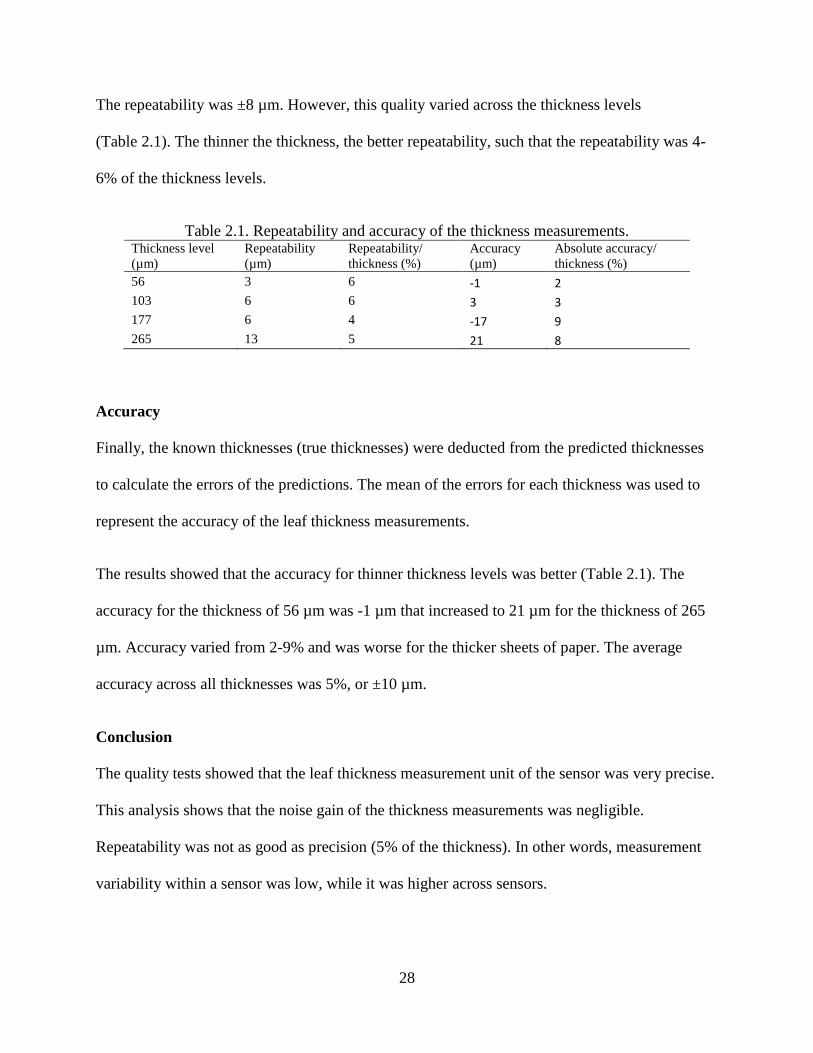
28
The repeatability was ±8 µm. However, this quality varied across the thickness levels
(Table 2.1). The thinner the thickness, the better repeatability, such that the repeatability was 4-
6% of the thickness levels.
Table 2.1. Repeatability and accuracy of the thickness measurements. Thickness level
(µm)
Repeatability
(µm)
Repeatability/
thickness (%)
Accuracy
(µm)
Absolute accuracy/
thickness (%)
56 3 6 -1 2
103 6 6 3 3
177 6 4 -17 9
265 13 5 21 8
Accuracy
Finally, the known thicknesses (true thicknesses) were deducted from the predicted thicknesses
to calculate the errors of the predictions. The mean of the errors for each thickness was used to
represent the accuracy of the leaf thickness measurements.
The results showed that the accuracy for thinner thickness levels was better (Table 2.1). The
accuracy for the thickness of 56 µm was -1 µm that increased to 21 µm for the thickness of 265
µm. Accuracy varied from 2-9% and was worse for the thicker sheets of paper. The average
accuracy across all thicknesses was 5%, or ±10 µm.
Conclusion
The quality tests showed that the leaf thickness measurement unit of the sensor was very precise.
This analysis shows that the noise gain of the thickness measurements was negligible.
Repeatability was not as good as precision (5% of the thickness). In other words, measurement
variability within a sensor was low, while it was higher across sensors.
29
In addition, the measurements were accurate for thin thicknesses while its quality decreased for
thicker thicknesses, such that the overall accuracy was moderately reliable (5% of the actual
thickness).
It is worth to mention that precision is the essential quality of a sensor for desired applications,
compared to accuracy and repeatability. In a real world applications, the actual leaf thickness is
not the most important information. Since the variability of leaf thickness across leaves of a
species is high (Carpenter & Smith, 1979; Hanba, Miyazawa, & Terashima, 1999; Nicotra et al.,
2011; Taiz & Zeiger, 2006), relative leaf thickness (normalized by the full-turgor thickness) was
used in previous studies of the relationship of leaf thickness versus leaf water content/potential
(Búrquez, 1987; Neumann et al., 1974; Scoffoni et al., 2014; Seelig et al., 2011). Other studies
employed the percent leaf shrinkage as an indicator of changes in the leaf water condition
(Búrquez, 1987; Neumann et al., 1974; Scoffoni et al., 2014; Seelig et al., 2011).
In conclusion, the high precision of the developed sensors supports the notion that the sensor is
suited to measure leaf thickness to determine plant water status.
References
Búrquez, A. (1987). Leaf thickness and water deficit in plants: a tool for field studies. Journal of
Experimental Botany, 38(186), 109–114.
Carpenter, S. B., & Smith, N. D. (1979). Variation in shade leaf thickness among urban trees
growing in metropolitan Lexington, Kentucky. Castanea, 44(2), 94–98.
Hanba, Y. T., Miyazawa, S.-I., & Terashima, I. (1999). The influence of leaf thickness on the
CO2 transfer conductance and leaf stable carbon isotope ratio for some evergreen tree

30
species in Japanese warm-temperate forests. Functional Ecology, 13(5), 632–639.
Neumann, H. H., Thurtell, G. W., Stevenson, K. R., & Beadle, C. L. (1974). Leaf water content
and potential in corn, sorghum, soybean, and sunflower. Canadian Journal of Plant
Science, 54(1), 185–195.
Nicotra, A. B., Leigh, A., Boyce, C. K., Jones, C. S., Niklas, K. J., Royer, D. L., & Tsukaya, H.
(2011). The evolution and functional significance of leaf shape in the angiosperms.
Functional Plant Biology, 38, 535–552.
Scoffoni, C., Vuong, C., Diep, S., Cochard, H., & Sack, L. (2014). Leaf shrinkage with
dehydration: coordination with hydraulic vulnerability and drought tolerance. Plant
Physiology, 164(4), 1772–1788.
Seelig, H. D., Stoner, R. J., & Linden, J. C. (2011). Irrigation control of cowpea plants using the
measurement of leaf thickness under greenhouse conditions. Irrigation Science, 30(4), 247–
257.
Taiz, L., & Zeiger, E. (2006). Plant Physiology (4th ed.). Sunderland, MA: Sinauer Associates.

31
Chapter 3: Leaf thickness to predict plant water status

32
Leaf thickness to predict plant water status
Abstract
Plant-based techniques to measure crop water status offer advantages over soil-based methods.
The objective of this study was to quantify the relationship between leaf thickness
measurements, as a promising plant-based technique, with leaf relative water content (RWC) and
assess the model across different species and leaf positions. The relationship between RWC and
relative thickness (RT) was determined on corn (Zea mays L.), sorghum (Sorghum bicolor (L.)
Moench), soybean (Glycine max (L.) Merr.), and fava bean (Vicia faba L.). RWC was calculated
as measured leaf water content/leaf water content at full turgor, and RT was measured as leaf
thickness/leaf thickness at full turgor. Two leaves from the top, middle, and bottom of five plants
of each species were collected at 60 days of age. Leaf samples brought to full turgor were left to
dehydrate in a lab. Leaf thickness was measured using a magnetic field sensor and water content
using weight loss. The RWC-RT relationship showed a distinct breakpoint, which we
hypothesize coincides with the turgor loss point. Piecewise linear modeling was used to regress
RWC versus RT, resulted in models explaining 86-97% of the variation. The precision was
improved by including leaf position in the model. The piecewise model parameters were related
to salt tolerance of the species, which is also an indicator of drought resistance. Generally, the
species with greater drought and salinity tolerance had a larger RT at the breakpoint.
Keywords: leaf thickness sensor; water stress; plant water status; drought tolerance; leaf
structure; piecewise model.

33
Symbols and abbreviations
Nomenclature
a The portion of the graph over which the data points of relative thickness are
equal to or smaller than the Relative Thickness at the breakpoint
b1 The portion of the graph over which the the data points of relative thickness are
greater than the Relative Thickness at the breakpoint
b2 The portion of the graph over which the the data points of relative thickness are
equal to or smaller than the Relative Thickness at the breakpoint
c The leaf relative thickness at the breakpoint of the piecewise linear model of
leaf relative water content versus leaf relative thickness
TLP Turgor loss point
RT Leaf relative thickness
RWC Leaf relative water content
Introduction
Increasing extraction of freshwater resources for various human needs is causing distress on all
continents. More than 50% of the U.S. has been facing drought for several years (Luebehusen,
2014). Improved water use efficiency in agriculture is one of the major ways to alleviate the
demand for freshwater, considering that 70% of globally extracted freshwater is used for
agriculture, primarily for irrigation (FAO, 2016). To improve water use efficiency in crop
production, it is necessary to determine when crops need water. The common methods of plant
water status estimation for practical applications are either based on evapotranspiration models
or soil moisture/potential measurements. Plant water is related to evapotranspiration and soil
moisture through complicated functions with several factors, such as stomatal behavior and root

34
geometry (Damour, Simonneau, Cochard, & Urban, 2010; Vogel, Votrubova, Dusek, & Dohnal,
2016). Evapotranspiration models typically require many weather and crop input data which are
often estimated, resulting in reduced accuracy. Soil water methods usually assume that wilting
point and field capacity are the same for all crops and that irrigation needs to start at 50% of the
difference. However, this ignores the fact that crops differ in their ability to extract water from
the soil and in their stomatal behavior to regulate the transpiration rate.
Instead of improving soil moisture measurement methods or evapotranspiration models, it
would, therefore, be much better if the critical water stress points at which irrigation should start
could be directly measured on the crops grown. Generally, plant-based approaches offer a more
reliable plant water status estimation by reducing the complexity associated with soil-plant-
atmosphere water relationship. In this study, we set out to determine if leaf thickness could be a
reliable indicator of water status of a plant.
Bachmann (1922) was the first to report that leaf thickness decreases upon dehydration and
increases upon rehydration. Subsequently, Meidner (1952) determined that there is a strong
correlation between leaf thickness and relative water content (RWC). Búrquez (1987) reported a
strong correlation between RWC and leaf thickness in Brassica napus L., Mirabilis jalapa L.,
Phaseolus vulgaris L., and Impatiens parviflora DC. These researchers measured leaf thickness
using different types of calipers and micrometers. Meidner (1952) used a gear-wheel micrometer
and Búrquez (1987) used a spring-loaded gear-wheel. These devices were bulky and hard to
automate to enable continuous plant water stress sensing. Transducer-based techniques were
explored to enable automated leaf thickness measurement (Dongsheng, Manxi, Huijuan, &
Ziqian, 2007; Li & Song, 2009; Malone, 1993; Marenco, Antezana-Vera, & Nascimento, 2009;
McBurney, 1992; Rozema, Arp, Diggelen, Kok, & Letschert, 1987; Syvertsen & Levy, 1982;
35
Vile et al., 2005; White & Montes-R, 2005). Most of these sensors are relatively bulky linear
variable displacement transducers (LVDT).
Sharon and Bravdo (1996) and Seelig, Stoner, and Linden (2011) developed small leaf thickness
sensors to optimize irrigation scheduling. Sharon and Bravdo (1996) compared irrigation
scheduling using continuous leaf thickness monitoring with four conventional drip irrigation
regimes based on timetables and water depletion. In this 4-year study, the sensor-based drip
irrigation treatment resulted in the highest yield and greatest water use efficiency of grapefruit
cv. Oroblanco (Citrus x paradisi Macfad). Similarly, Seelig et al. (2011) were able to improve
water use efficiency of irrigated cowpea 25 to 45% by an automated irrigation system based on a
leaf thickness sensor compared with timed irrigation scheduling. These studies show that
irrigation scheduling based on the automated leaf thickness sensing has the potential to improve
water use efficiency and conserve irrigation water.
The relationship between leaf thickness and RWC depends on plant and leaf characteristics and
is affected by environmental variables. Leaf thickness is determined by plant anatomy, including
the number, size, and arrangement of leaf cells that differ among species (Carpenter & Smith,
1979; Nicotra et al., 2011; Taiz & Zeiger, 2006; Vogelmann, Bornman, & Yates, 1996). Giuliani
et al. (2013) have reported a significant difference in leaf anatomy among species of the genus
Oryza. There is a significant variation in the structure of leaf mesophyll even between leaves
located at different positions on the same plant (Eames & MacDaniels, 1925). The number and
arrangement of the palisade parenchyma, as well as the overall morphology of a leaf, vary
between species. They also depend on environmental variables such as light exposure,
temperature, age, and irrigation regimes (Abrams & Kubiske, 1990; Búrquez, 1987; Carpenter &
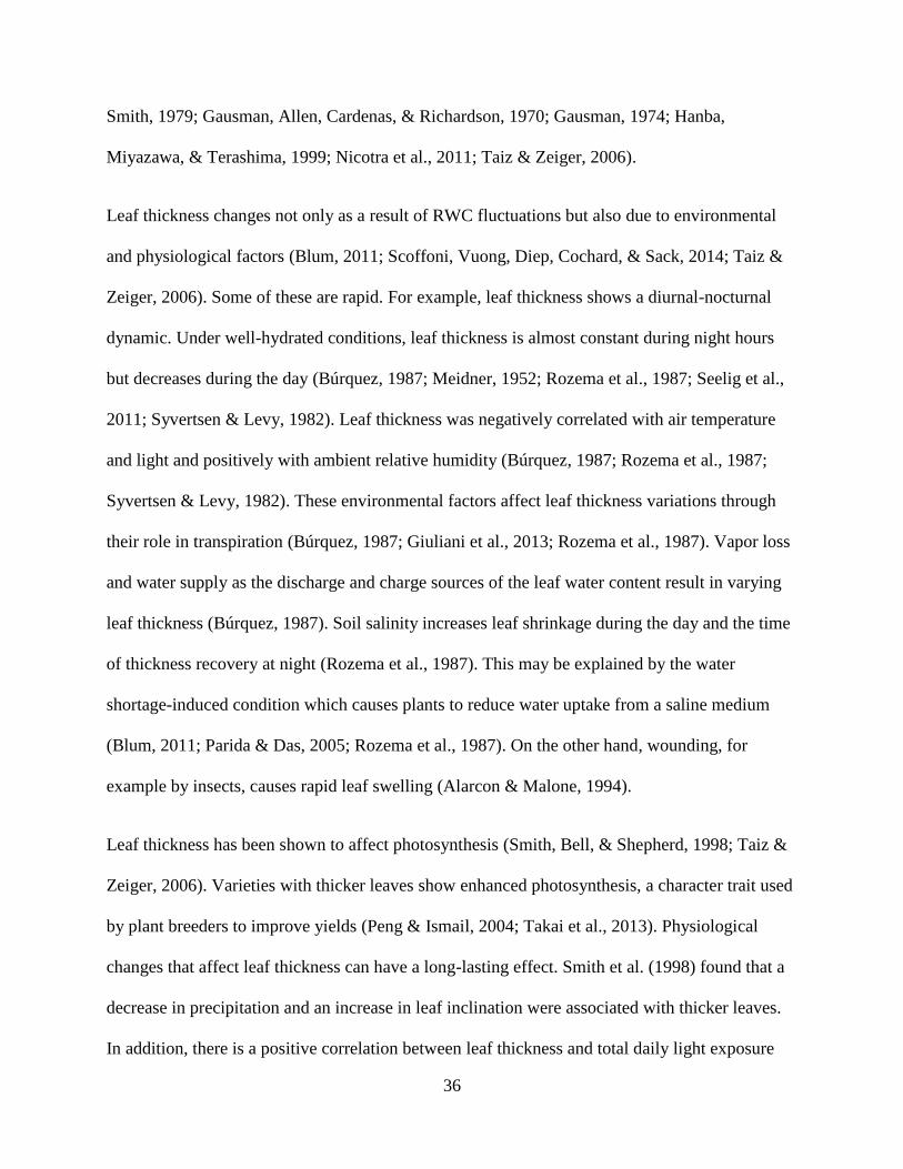
36
Smith, 1979; Gausman, Allen, Cardenas, & Richardson, 1970; Gausman, 1974; Hanba,
Miyazawa, & Terashima, 1999; Nicotra et al., 2011; Taiz & Zeiger, 2006).
Leaf thickness changes not only as a result of RWC fluctuations but also due to environmental
and physiological factors (Blum, 2011; Scoffoni, Vuong, Diep, Cochard, & Sack, 2014; Taiz &
Zeiger, 2006). Some of these are rapid. For example, leaf thickness shows a diurnal-nocturnal
dynamic. Under well-hydrated conditions, leaf thickness is almost constant during night hours
but decreases during the day (Búrquez, 1987; Meidner, 1952; Rozema et al., 1987; Seelig et al.,
2011; Syvertsen & Levy, 1982). Leaf thickness was negatively correlated with air temperature
and light and positively with ambient relative humidity (Búrquez, 1987; Rozema et al., 1987;
Syvertsen & Levy, 1982). These environmental factors affect leaf thickness variations through
their role in transpiration (Búrquez, 1987; Giuliani et al., 2013; Rozema et al., 1987). Vapor loss
and water supply as the discharge and charge sources of the leaf water content result in varying
leaf thickness (Búrquez, 1987). Soil salinity increases leaf shrinkage during the day and the time
of thickness recovery at night (Rozema et al., 1987). This may be explained by the water
shortage-induced condition which causes plants to reduce water uptake from a saline medium
(Blum, 2011; Parida & Das, 2005; Rozema et al., 1987). On the other hand, wounding, for
example by insects, causes rapid leaf swelling (Alarcon & Malone, 1994).
Leaf thickness has been shown to affect photosynthesis (Smith, Bell, & Shepherd, 1998; Taiz &
Zeiger, 2006). Varieties with thicker leaves show enhanced photosynthesis, a character trait used
by plant breeders to improve yields (Peng & Ismail, 2004; Takai et al., 2013). Physiological
changes that affect leaf thickness can have a long-lasting effect. Smith et al. (1998) found that a
decrease in precipitation and an increase in leaf inclination were associated with thicker leaves.
In addition, there is a positive correlation between leaf thickness and total daily light exposure

37
(Abrams & Kubiske, 1990; Carpenter & Smith, 1981; Eames & MacDaniels, 1925; Nobel &
Hartsock, 1981; Smith et al., 1998; Yun & Taylor, 1986). Nobel and Hartsock (1981) reported a
positive correlation between leaf thickness and leaf age.
A number of researchers have worked on the relationship between leaf thickness and leaf
structural and functional traits (Giuliani et al., 2013; Patakas & Noitsakis, 1997; Sack &
Scoffoni, 2012; Scoffoni et al., 2014). Leaf thickness was positively correlated with leaf
hydraulic conductivity (Scoffoni et al., 2014) and elastic modulus (Aasamaa, Niinemets, &
Sõber, 2005; Scoffoni et al., 2014). Drought results in cell wall hardening and larger elastic
modulus which helps the tissue maintain turgor pressure and avoid water stress (Blum, 2011;
Martinez et al., 2007). Salinity decreased the epidermal and mesophyll thickness of mangrove B.
parviflora leaves (Parida et al., 2004). The tight relationship between leaf thickness and leaf
water potential (𝜓𝑙𝑒𝑎𝑓) was shown in several studies (Búrquez, 1987; McBurney, 1992;
Neumann et al., 1974; Scoffoni et al., 2014; Syvertsen & Levy, 1982).
In summary, earlier work suggests leaf thickness measurement to be a feasible technique for
estimation of plant water status. However, the earlier studies lack models to quantify the
relationship between leaf thickness and RWC. In practical applications (e.g. irrigation timing),
using leaf thickness measurements as means for estimation of plant water status requires the
identification of a model which determines both the plant water condition and the best time for
irrigation. In addition, as mentioned earlier, leaf thickness is a function of leaf structural traits
which may vary by species and leaf position on the plant. Therefore, another question is whether
species and leaf position on the plant influence the leaf thickness - leaf water content
relationship.

38
Therefore, the objective of this study was to determine the relationship between RWC and leaf
relative thickness (RT) for different species. The species were selected from dicotyledons and
monocotyledons with different drought tolerances to study their differences in the RWC-RT
relationship. This study also considered the extent to which leaf location on a plant impacted the
relationship.
Materials and methods
Plant cultivation
Corn (Zea mays L.), sorghum (Sorghum bicolor (L.) Moench), soybean (Glycine max (L.)
Merr.), and fava bean (Vicia faba L.) were grown under controlled conditions in a greenhouse at
the Pennsylvania State University, University Park, Pennsylvania. Fifteen plants of each crop
were grown under a mixture of natural and artificial light to generate a photoperiod of 15 hours,
day/night temperatures of 27/18 °C, relative humidity of 60% (±20%), and were irrigated every
three days to saturation and allowed to drain –a growing condition without stress.
Leaf sampling
Sixty days after seeding, the pots were irrigated to saturation and allowed to drain for eight hours
before collecting the leaves. Two leaves were selected from the top, middle and bottom of five
randomly selected plants of each species (30 leaves within species, 120 leaves in total for the
four species). The petioles of the cut leaves were immediately submerged in distilled water and
the entire leaves and the container holding the water were enclosed in dark polyethylene bags.
These bags were stored in the dark at 7 °C for eight hours in a refrigerator to ensure that leaves
reached full turgidity (Búrquez, 1987).

39
Two 225 mm2 samples were taken from the center of a leaf (avoiding the edges and major veins)
under lab conditions (25 °C and relative humidity of 40 ±5%). One sample was used for
continuous leaf thickness measurement and the other sample was used for continuous leaf
weighing. This method was chosen because it was not possible to simultaneously weigh the
sample with the sensor attached to it due to wiring attaching the sensor to the data logger. In
addition, the aim was to not remove the leaf thickness sensor in order to prevent possible leaf
damage, loss of data continuity, and spikes or drops in thickness measured due to repositioning
the sensor. Preliminary data confirmed the assumption that the rate of water loss over time was
not significantly different between two leaf pieces dehydrating under the same conditions in the
lab.
Leaf thickness and water content measurement
Leaf thickness was measured by a developed leaf thickness sensor using a magnetic field sensor
and two permanent magnets that were fixed on a clear rigid clip (Fig. 3.1). One of the magnets
and the magnetic field sensor were fixed on opposite sides of the clip. The voltage output of the
magnetic field sensor varied based on the distance from this magnet enabling continuous leaf
thickness measurement. The second magnet was fixed under the magnetic field sensor with the
polarity opposite that of the other magnet to reduce the offset magnetic field. This magnet helps
to avoid sensor saturation for very small thicknesses while still allowing high resolution. Sensor
calibration using paper sheets of known thickness showed a coefficient of determination of 0.97.
Sensor output was recorded at one-minute intervals using a DT85M data logger (DataTaker,
Melbourne, Australia).
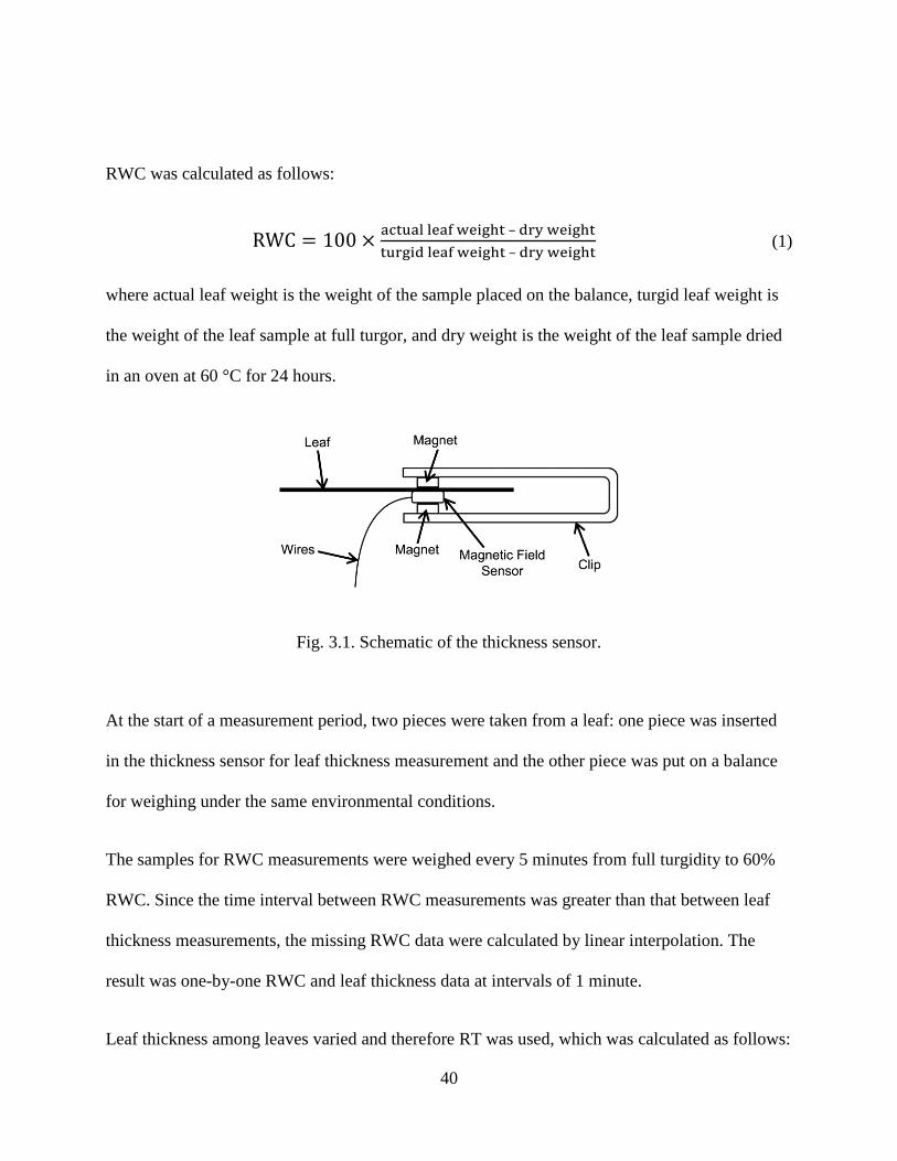
40
RWC was calculated as follows:
RWC = 100 ×actual leaf weight – dry weight
turgid leaf weight – dry weight (1)
where actual leaf weight is the weight of the sample placed on the balance, turgid leaf weight is
the weight of the leaf sample at full turgor, and dry weight is the weight of the leaf sample dried
in an oven at 60 °C for 24 hours.
Fig. 3.1. Schematic of the thickness sensor.
At the start of a measurement period, two pieces were taken from a leaf: one piece was inserted
in the thickness sensor for leaf thickness measurement and the other piece was put on a balance
for weighing under the same environmental conditions.
The samples for RWC measurements were weighed every 5 minutes from full turgidity to 60%
RWC. Since the time interval between RWC measurements was greater than that between leaf
thickness measurements, the missing RWC data were calculated by linear interpolation. The
result was one-by-one RWC and leaf thickness data at intervals of 1 minute.
Leaf thickness among leaves varied and therefore RT was used, which was calculated as follows:

41
RT = leaf thickness measured / leaf thickness at full turgor (2)
Statistical analysis
Minitab 16.0 was employed for ANOVA and regression of RWC vs. RT while SAS 9.3 was used
for piecewise linear regression as described by Ryan and Porth (2007).
Results and discussion
RWC-RT relationship
The RWC-RT relationship of each species is shown in Fig. 3.2. The RWC-RT curve showed a
sudden change in slope at a point we refer to as the “breakpoint”. This breakpoint was also
observed in other studies and is known as the turgor loss point (TLP), the point at which leaf turgor
pressure is equal to zero bar (Begg et al., 1964; Lenz, Wright, & Westoby, 2006; Neumann et al.,
1974; Sanchez-Diaz & Kramer, 1971; Scoffoni et al., 2014; Stoyanov, 2005).
Therefore, piecewise linear regression modeling was applied to the trends of RWC-RT (equation
3).
RWC = { 𝑎 + 𝑐(𝑏2 − 𝑏1) + 𝑏1RT, RT > 𝑐 (𝑝ℎ𝑎𝑠𝑒 1)
𝑎 + 𝑏2RT, RT ≤ 𝑐 (𝑝ℎ𝑎𝑠𝑒 2) (3)
where a is the intercept with the y-axis (RWC) of the regression line below the breakpoint, c is the
RT at the breakpoint, b1 is the slope of the line at RT>c, and b2 is the slope of the line at RT≤c.
Parameter estimates are shown in Tables 3.1 and 3.2.

42
Fig. 3.2. Fitted piecewise models of leaf relative water content (RWC) vs. leaf relative thickness
(RT) for corn (A), sorghum (B), soybean (C), and fava bean (D). The solid lines show the
piecewise regression lines. The gray points display the observations.
Table 3.1. Estimated parameters for the piecewise regression models of leaf relative water
content (RWC) vs. leaf relative thickness (RT) for different species. c is the RT at the breakpoint
of the piecewise model, b1 and b2 are the slopes of the model for respectively RT > c and RT ≤ c,
and a is the model intercept for RT ≤ c.
Species b1 c b2 a R2 P-value
Estimated
RWC at c
Corn 0.166
±0.113
0.672
±0.024
1.050
±0.051
0.208
±0.025
0.86 <0.001 91%
Sorghum 0.348
±0.075
0.750
±0.013
1.156
±0.032
0.032
±0.020
0.97 <0.001 90%
Soybean 0.322
±0.063
0.653
±0.024
0.935
±0.044
0.247
±0.022
0.93 <0.001 86%
Fava bean 0.192
±0.064
0.517
±0.029
0.885
±0.063
0.407
±0.021
0.89 <0.001 86%
Note: The margins of error are calculated based on a 95% confidence interval.

43
Table 3.2. Estimated parameters for the piecewise regression models of leaf relative water
content (RWC) vs. leaf relative thickness (RT) across leaf locations of the species. c is the RT at
the breakpoint of the piecewise model, b1 and b2 are the slopes of the model for respectively RT
> c and RT ≤ c, and a is the model intercept for RT ≤ c.
Species
Leaf
location b1 c b2 a R2 P-value
Estimated
RWC at c
Corn Top 0.229
±0.150
0.557
±0.025
1.435
±0.107
0.070
±0.056
0.99 <0.001 87%
Middle 0.169
±0.036
0.635
±0.007
1.220
±0.021
0.142
±0.010
0.99 <0.001 92%
Bottom 0.223
±0.022
0.662
±0.005
1.334
±0.029
0.015
±0.013
0.90 <0.001 90%
Sorghum Top 0.452
±0.059
0.694
±0.007
1.115
±0.021
0.075
±0.013
> 0.99 <0.001 85%
Middle 0.380
±0.036
0.728
±0.006
1.247
±0.020
-0.020
±0.012
> 0.99 <0.001 89%
Bottom 0.276
±0.022
0.766
±0.007
1.353
±0.018
-0.110
±0.010
> 0.99 <0.001 93%
Soybean Top 0.289
±0.045
0.650
±0.016
0.976
±0.066
0.248
±0.033
0.98 <0.001 88%
Middle 0.282
±0.025
0.637
±0.008
1.038
±0.021
0.209
±0.010
> 0.99 <0.001 87%
Bottom 0.379
±0.049
0.611
±0.017
1.118
±0.033
0.116
±0.016
0.98 <0.001 80%
Fava bean Top 0.239
±0.022
0.487
±0.011
1.236
±0.056
0.242
±0.016
0.91 <0.001 84%
Middle 0.211
±0.042
0.425
±0.013
1.314
±0.078
0.289
±0.024
0.97 <0.001 85%
Bottom 0.257
±0.082
0.394
±0.031
1.100
±0.166
0.374
±0.061
0.99 <0.001 81%
Note: The margins of error are calculated based on a 95% confidence interval.
The slope of the line at the early stages of dehydration (b1) was much smaller than the slope of the
line at the later stages of dehydration (b2). This means that a large change in RT accompanied a
small change in RWC at early stages of dehydration, while a small change of RT accompanied a
large change in RWC at later stages of dehydration. This result is in agreement with the results of
Sancho-Knapik et al. (2011) on Quercus muehlenbergii Engelm. They reported that a breakpoint

44
at the TLP occurred in the relationship of RWC and leaf thickness such that the changes of RWC
for a given decrement in leaf thickness from full turgor to TLP was small in comparison with that
below TLP. In addition, Scoffoni et al. (2014) observed a breakpoint at the TLP in the relationship
between leaf thickness and 𝜓𝑙𝑒𝑎𝑓. These results imply that the observed breakpoint in our study
occurred at TLP.
Estimated model parameters by species
Table 3.1 shows the estimated model parameters for each species, averaged over leaf locations.
Large differences were observed among the estimated model parameters of the species. The slope
of the regression line in phase 1 (b1) was greatest for sorghum, followed by soybean, fava bean
and smallest for corn. In phase 1, in sorghum, RT changed least with a given change of RWC,
while it changed most with a unit change of RWC in corn. The slope b1 of soybean was similar to
that of sorghum while b1 of fava bean was similar to that in corn. The breakpoint c occurred at the
largest RT in sorghum, followed by corn, soybean, and fava bean. The slope of the line in phase 2
(b2) was largest for sorghum, followed by corn, soybean, and smallest for fava bean.
The results show that the relationship between RWC-RT needs to be determined for each species
separately.
The dynamics of the RWC-RT relationship can possibly provide information about species’
drought tolerance. The greatest differences between the estimated slopes and breakpoint occurred
between sorghum and fava bean. Sorghum had the greatest slopes in both phases and the highest
RT at the breakpoint c. Fava bean, on the other hand, had the smallest b2, the smallest c, and the
second smallest b1. Sorghum is among the most drought tolerant cultivated crops (Sabadin et al.,
2012). Fava bean, on the other hand, is known for its lack of drought tolerance (Multari, Stewart,

45
& Russell, 2015). This observation is in agreement with Scoffoni et al. (2014) who reported that
the thickness of leaves of moist habitat species decreased more from full-turgor to TLP compared
with the leaves of dry habitat species better adapted to drought. This result is comparable with a
smaller c for drought-sensitive species while drought-tolerant species would have a larger c. This
interpretation implies that the drought tolerance of corn and soybean is intermediate between
sorghum and fava bean.
The larger RT at the breakpoint c of drought tolerant species would be explained by the relationship
between cell rigidity and drought tolerance. Cell wall rigidity is expressed as one of the drought
tolerance mechanisms by maintaining cell structure at lower water potentials (Blum, 2011;
Giuliani et al., 2013; Patakas & Noitsakis, 1997).
Monocotyledons versus dicotyledons
RT at the breakpoint c, the slope b2, and RWC at c were larger for the monocot (monocotyledon)
species than for the dicot (dicotyledon) species. These differences may reflect leaf anatomical
differences, specifically bulk leaf rigidity, between monocots and dicots. In contrast to the dicots,
the monocot leaves contain dense longitudinal main veins and silica deposition providing
mechanical strength to their long leaves (Read & Stokes, 2006). These effects seem to be more
pronounced below the TLP, suggesting a reason that b1 of monocots was not consistently larger
than that of dicots.
Thicker cell walls, greater lignin content in the vascular tissues (Myburg & Sederoff, 2001; Sack
& Scoffoni, 2013) and higher silica content (Read & Stokes, 2006), result in a more rigid bulk leaf
blade in the monocots than in dicots. A more rigid leaf structure of monocots would explain their
larger slopes b2 representing a smaller rate of RT change with a unit change in RWC below the

46
breakpoint. Hence, a cell with a rigid structure reaches TLP with less RT shrinkage and RWC loss
(Neumann et al., 1974; Scoffoni et al., 2014), the monocot leaves with more rigid structure would
shrink less and lose less RWC from full-turgor to TLP, explaining the larger RT and RWC at c.
RWC-RT model and salt tolerance
Salt tolerance of a species is characterized by a threshold EC below which crop yield is not
affected. The relationship between threshold EC levels for these species and model parameters
were therefore investigated. Salinity thresholds for corn came from Bernstein and Ayers (1949)
and Kaddah and Ghowail (1964), for sorghum from Francois et al. (1984), for soybeans from
Abel and MacKenzie (1964), Bernstein et al. (1955), and Bernstein and Ogata (1966), and for
fava bean from Ayers and Eberhard (1960). The slope b1 was strongly correlated with the salinity
thresholds (Fig. 3.3-A). The crops with higher thresholds tended to have greater RT values at the
breakpoint c and slopes b2 (Fig. 3.3-B and Fig. 3.3-C).
Salinity reduces soil water osmotic potential which impedes water uptake, increasing drought
stress (Taiz & Zeiger, 2006). Leaf elasticity and crop salt tolerance may be correlated since water
stress and water salinity have similar effects on leaf anatomy (Parida & Das, 2005) and salt and
drought tolerant species share common structural traits (Blum, 2011; Giuliani et al., 2013; Parida
& Das, 2005; Rhizopoulou & Psaras, 2003; Taiz & Zeiger, 2006).
These results suggest that the crop with a smaller decrease of RT with a unit decrease of RWC in
both phases (i.e. the crop with the smaller slope) and a larger c has a higher salt tolerance threshold.
The effect of cell wall rigidity may explain the positive correlation between the piecewise
parameters and the salinity threshold. Cell wall rigidity is one of the mechanisms of salt-tolerant
species to maintain cell structure at low water potentials (Gall et al., 2015; Morgan, 1986;

47
Zagorchev, Kamenova, & Odjakova, 2014). Therefore, a smaller rate of decrease of leaf thickness
with leaf moisture loss implies a more rigid bulk structure and accordingly higher salt tolerance.
Fig. 3.3. The relationship between piecewise linear model parameters of leaf relative water
content-relative thickness (RT) with soil electrical conductivity (EC) threshold (maximum EC
that does not result in yield loss) for corn (▲), sorghum (■), soybean (○), and fava bean (●). c is
the RT at the breakpoint of the piecewise model, and b1 and b2 are the slopes of the model for
respectively RT > c and RT ≤ c. A) b1 vs. threshold (y = 0.035x + 0.126; R² = 0.95; p-value =
0.02), B) c vs. threshold (y = 0.028x + 0.542; R² = 0.54; p-value = 0.26), C) b2 vs. threshold (y =
0.027x + 0.903; R² = 0.33; p-value = 0.42). The references for the EC threshold data of the crops
are cited in the text.

48
Effect of leaf location on the RWC-RT relationship
Table 3.2 shows the estimated piecewise parameters across the leaf locations on the plants. Leaf
location had a significant effect on most parameters of the RWC vs. RT relationship of all four
species. Leaf location significantly affected b1 for all the species, the breakpoint c for corn and
sorghum, and b2 and a for soybean and fava bean (Table 3.3).
Table 3.3. The significance of leaf location as a factor in the variability of the piecewise model
parameters of leaf relative water content vs. leaf relative thickness (RT). c is the RT at the
breakpoint of the piecewise model, b1 and b2 are the slopes of the model for respectively RT > c
and RT ≤ c, and a is the model intercept for RT ≤ c.
P-value
Species b1 c b2 a
Corn <0.01 0.01 0.51 0.66
Sorghum <0.01 0.01 0.20 0.21
Soybean 0.04 0.80 <0.01 <0.01
Fava bean 0.01 0.49 <0.01 0.01
Evidently, the effects of leaf position on model parameters varied by species. Leaf position reflects
leaf age and light exposure which affect leaf structural traits. Sylvester (2001) reported a
significant effect of age on the leaf anatomy of corn, rice, and bluegrass. Aging causes cell wall
thickening and increased elastic modulus (Lambers, Chapin, & Pons, 2008; Patakas & Noitsakis,
1997). The penetration of sunlight decreases from top to bottom of a canopy (Jones, 2014). In our
study, the plants were spaced sufficiently close together such that upper leaves shaded lower
leaves. Exposure to sunlight has a strong influence on the leaf structure resulting in the sun- and
shade-type leaves (Smith et al., 1998). Vogelmann et al. (1996) showed that sun leaves of
Thermopsis montana had longer palisade cells and were much thicker than shade leaves. The cell
49
walls of sun leaves have higher lignin content and greater rigidity than shade leaves (Gall et al.,
2015).
The breakpoint c of monocots was higher for the top than the lower leaves while this trend was
reversed for the dicots. The growth pattern of monocots implies that the older leaves are at the
bottom while younger leaves are at the top. Since age affects cell wall rigidity (Nobel, 2009;
Patakas & Noitsakis, 1997), the lower leaves of the monocots are expected to have more rigid bulk
structure than the higher leaves. This may help explain why lower leaves of the monocots had a
larger c. On the other hand, the growth pattern of dicot species does not ensure the vertical age
distribution of leaves. The plant grows vertically along the main stem and laterally by branching.
Therefore, random selection of leaves within leaf locations does not assure the order of leaf ages
along the main stem. However, the contrast between shade and light leaves may explain the order
of the breakpoints for the dicots. Light exposure of leaves of monocot species at lower levels in
the canopy may not decrease as much as in dicots because upright leaf position allows more light
penetration (Read & Stokes, 2006). On the other hand, the cell wall lignin content and the bulk
elastic modulus of sun leaves are greater than shade leaves (Gall et al., 2015). Therefore, it appears
that the leaves near the top of the dicots had more rigid cells, resulting in less shrinkage and lower
c values.
Conclusion
This study shows that leaf thickness can be used to measure leaf relative water content. We
observed an abrupt increase of the slope of the RWC-RT curve as leaves dried out. Piecewise
linear regression resulted in models that explained 86-97% of the variation of RWC-RT
relationship of the four species studied. We suggest that the factor c in these models represents the

50
RT at the TLP. The relationship between RT and RWC varied by species and leaf location. To use
leaf thickness as an estimate of leaf water content, it is, therefore, necessary to develop models
that vary by species and leaf location. It is recognized that model calibrations will change as leaves
age - a top leaf may become a middle leaf later. Additionally, environmental factors such as light,
temperature, relative humidity, disease, and pest pressure may affect leaf thickness as well.
Additional work, building on this research accounting for some of these environmental factors will
help develop practical models for use in the field. We suggest that the RWC-RT curves can provide
information about drought and salt tolerance of species. If it is true that the breakpoint c represents
TLP, the breakpoint implies a critical water stress level which leads to a dramatic change in the
leaf physiology. This information can be used to screen species and varieties for drought and
salinity tolerance. In addition, this knowledge can be used to develop leaf thickness sensors that
can be used to monitor plant water stress for irrigation scheduling and drought monitoring.
References
Aasamaa, K., Niinemets, U., & Sõber, A. (2005). Leaf hydraulic conductance in relation to
anatomical and functional traits during Populus tremula leaf ontogeny. Tree Physiology, 25,
1409–1418.
Abel, G. H., & MacKenzie, A. J. (1964). Salt tolerance of soybean varieties (Glycine max L.
Merrill) during germination and later growth. Crop Science, 4, 157–161.
Abrams, M., & Kubiske, M. (1990). Leaf structural characteristics of 31 hardwood and conifer
tree species in central Wisconsin: influence of light regime and shade-tolerance rank. Forest
Ecology and Management, 31, 245–253.

51
Alarcon, J., & Malone, M. (1994). Substantial hydraulic signals are triggered by leaf-biting
insects in tomato. Journal of Experimental Botany, 45(276), 953–957.
Ayers, A. D., & Eberhard, D. L. (1960). Response of edible broadbean to several levels of
salinity. Agronomy Journal, 52, 110–111.
Bachmann, F. (1922). Studien über die dickenänderung von laubblättern. Jahrbücher Für
Wissenschaftliche Botanik, 61, 372–429.
Begg, J. E., Bierhuizen, J. F., Lemon, E. R., Misra, D. K., Slatyer, R. O., & Stern, W. R. (1964).
Diurnal energy and water exchanges in bulrush millet in an area of high solar radiation.
Agricultural Meteorology, 1(4), 294–312.
Bernstein, L., & Ayers, A. D. (1949). Salt tolerance of sweet corn. Report to Collaborators.
Riverside, CA: United States Salinity Laboratory.
Bernstein, L., MacKenzie, A. J., & Krantz, B. A. (1955). Salt tolerance of field crops - soybeans.
Report to Collaborators. Riverside, CA: United States Salinity Laboratory.
Bernstein, L., & Ogata, G. (1966). Effects of salinity on nodulation, nitrogen fixation, and
growth of soybeans and alfalfa. Agronomy Journal, 58, 201–203.
Blum, A. (2011). Plant water relations, plant stress and plant production. Plant breeding for
water-limited environments (pp. 11–52). New York, NY: Springer New York.
Búrquez, A. (1987). Leaf thickness and water deficit in plants: a tool for field studies. Journal of
Experimental Botany, 38(186), 109–114.
Carpenter, S. B., & Smith, N. D. (1979). Variation in shade leaf thickness among urban trees

52
growing in metropolitan Lexington, Kentucky. Castanea, 44(2), 94–98.
Carpenter, S. B., & Smith, N. D. (1981). A comparative study of leaf thickness among southern
Appalachian hardwoods. Canadian Journal of Botany, 59(8), 1393–1396.
Damour, G., Simonneau, T., Cochard, H., & Urban, L. (2010). An overview of models of
stomatal conductance at the leaf level. Plant, Cell and Environment, 33(9), 1419–1438.
Dongsheng, L., Manxi, H., Huijuan, W., & Ziqian, W. (2007). Law of fluctuation in plant leaves
thickness during day and night. Journal of Physics: Conference Series, 48, 1447–1452.
Eames, A. J., & MacDaniels, L. H. (1925). An introduction to plant anatomy (1st ed.). New York,
NY: McGraw-Hill.
FAO. (2016). AQUASTAT website. Food and Agriculture Organization of the United Nations
(FAO). Retrieved April 22, 2016, from http://www.fao.org/nr/water/aquastat/water_use.
Francois, L. E., Donovan, T. J., & Maas, E. V. (1984). Salinity effects on seed yield, growth, and
germination of grain sorghum. Agronomy Journal, 82, 587–592.
Gall, H., Philippe, F., Domon, J.-M., Gillet, F., Pelloux, J., & Rayon, C. (2015). Cell wall
metabolism in response to abiotic stress. Plants, 4(1), 112–166.
Gausman, H. (1974). Leaf reflectance of near-infrared. Photogrammetric Engineering, 40, 183–
191.
Gausman, H. W., Allen, W. A., Cardenas, R., & Richardson, A. J. (1970). Relation of light
reflectance to histological and physical evaluations of cotton leaf maturity. Applied Optics,
9(3), 545–552.

53
Giuliani, R., Koteyeva, N., Voznesenskaya, E., Evans, M. A., Cousins, A. B., & Edwards, G. E.
(2013). Coordination of leaf photosynthesis, transpiration, and structural traits in rice and
wild relatives (genus Oryza). Plant Physiology, 162(3), 1632–51.
Hanba, Y. T., Miyazawa, S. I., & Terashima, I. (1999). The influence of leaf thickness on the
CO2 transfer conductance and leaf stable carbon isotope ratio for some evergreen tree
species in Japanese warm-temperate forests. Functional Ecology, 13(5), 632–639.
Jones, H. G. (2014). Plants and microclimate: a quantitative approach to environmental plant
physiology (3rd ed.). Cambridge: Cambridge University Press.
Kaddah, M. T., & Ghowail, S. I. (1964). Salinity effects on the growth of corn at different stages
of development. Agronomy Journal, 56, 214–217.
Lambers, H., Chapin, F. S., & Pons, T. L. (2008). Plant Physiological Ecology. New York:
Springer New York.
Lenz, T. I., Wright, I. J., & Westoby, M. (2006). Interrelations among pressure-volume curve
traits across species and water availability gradients. Physiologia Plantarum, 127(3), 423–
433.
Li, D., & Song, J. (2009). A novel irrigation system controlled by leaf thickness. In ASABE
Annual International Meeting. Reno, Nevada: American Society of Agricultural and
Biological Engineers (ASABE).
Luebehusen, E. (2014). Percent area in U.S. drought monitor categories. The National Drought
Mitigation Center, the U.S. Department of Agriculture, and the National Oceanic and

54
Atmospheric Administration. Retrieved July 12, 2016, from
http://droughtmonitor.unl.edu/MapsAndData/DataTables.aspx.
Malone, M. (1993). Rapid inhibition of leaf growth by root cooling in wheat: kinetics and
mechanism. Journal of Experimental Botany, 44(268), 1663–1669.
Marenco, R. A., Antezana-Vera, S. A., & Nascimento, H. C. S. (2009). Relationship between
specific leaf area, leaf thickness, leaf water content and SPAD-502 readings in six
Amazonian tree species. Photosynthetica, 47(2), 184–190.
Martinez, J. P., Silva, H., Ledent, J. F., & Pinto, M. (2007). Effect of drought stress on the
osmotic adjustment, cell wall elasticity and cell volume of six cultivars of common beans
(Phaseolus vulgaris L.). European Journal of Agronomy, 26(1), 30–38.
McBurney, T. (1992). The relationship between leaf thickness and plant water potential. Journal
of Experimental Botany, 43(248), 327–335.
Meidner, H. (1952). An instrument for the continuous determination of leaf thickness changes in
the field. Journal of Experimental Botany, 3(9), 319–325.
Morgan, J. a. (1986). The effects of N nutrition on the water relations and gas exchange
characteristics of wheat (Triticum aestivum L.). Plant Physiology, 80(1), 52–58.
Multari, S., Stewart, D., & Russell, W. R. (2015). Potential of fava bean as future protein supply
to partially replace meat intake in the human diet. Comprehensive Reviews in Food Science
and Food Safety, 14, 511–522.
Myburg, A. A., & Sederoff, R. R. (2001). Xylem structure and function. In Encyclopedia of Life

55
Sciences. Nature Publishing Group.
Neumann, H. H., Thurtell, G. W., Stevenson, K. R., & Beadle, C. L. (1974). Leaf water content
and potential in corn, sorghum, soybean, and sunflower. Canadian Journal of Plant
Science, 54(1), 185–195.
Nicotra, A. B., Leigh, A., Boyce, C. K., Jones, C. S., Niklas, K. J., Royer, D. L., & Tsukaya, H.
(2011). The evolution and functional significance of leaf shape in the angiosperms.
Functional Plant Biology, 38, 535–552.
Nobel, P. S. (2009). Physicochemical and environmental plant physiology (4th ed). San Diego:
Academic Press.
Nobel, P. S., & Hartsock, T. L. (1981). Development of leaf thickness for Plectranthus
parviflorus – influence of photosynthetically active radiation. Physiologia Plantarum,
51(2), 163–166.
Parida, A. K., & Das, A. B. (2005). Salt tolerance and salinity effects on plants: a review.
Ecotoxicology and Environmental Safety, 60(3), 324–349.
Parida, A. K., Das, A. B., & Mittra, B. (2004). Effects of salt on growth, ion accumulation,
photosynthesis and leaf anatomy of the mangrove, Bruguiera parviflora. Trees - Structure
and Function, 18(2), 167–174.
Patakas, A., & Noitsakis, B. (1997). Cell wall elasticity as a mechanism to maintain favorable
water relations during leaf ontogeny in grapevines. American Journal of Enology and
Viticulture, 48(3), 352–356.
56
Peng, S., & Ismail, A. M. (2004). Physiology basis of yield and environmental adaptation in rice.
In H. T. Nguyen & A. Blum (Eds.), Physiology and biotechnology integration for plant
breeding (pp. 72–118). New York: Marcel Dekker.
Read, J., & Stokes, A. (2006). Plant biomechanics in an ecological context. American Journal of
Botany, 93(10), 1546–1565.
Rhizopoulou, S., & Psaras, G. K. (2003). Development and structure of drought-tolerant leaves
of the Mediterranean shrub Capparis spinosa L. Annals of Botany, 92(3), 377–383.
Rozema, J., Arp, W., Diggelen, J., Kok, E., & Letschert, J. (1987). An ecophysiological
comparison of measurements of the diurnal rhythm of the leaf elongation and changes of the
leaf thickness of salt-resistant dicotyledonae and monocotyledonae. Journal of
Experimental Botany, 38(188), 442–453.
Ryan, S. E., & Porth, L. S. (2007). A tutorial on the piecewise regression approach applied to
bedload transport data. General technical report RMRS-GTR-189. General Technical
Report RMRS-GTR-189. Fort Collins, Colorado: U.S. Department of Agriculture, Forest
Service, Rocky Mountain Research Station. Retrieved on July 12, 2016, from
http://www.fs.fed.us/rm/pubs/rmrs_gtr189.pdf.
Sabadin, P. K., Malosetti, M., Boer, M. P., Tardin, F. D., Santos, F. G., Guimarães, C. T., …
Magalhaes, J. V. (2012). Studying the genetic basis of drought tolerance in sorghum by
managed stress trials and adjustments for phenological and plant height differences.
Theoretical and Applied Genetics, 124(8), 1389–1402.
Sack, L., & Scoffoni, C. (2012). Measurement of leaf hydraulic conductance and stomatal

57
conductance and their responses to irradiance and dehydration using the Evaporative Flux
Method (EFM). Journal of Visualized Experiments, 70(e4179). doi:10.3791/4179.
Sack, L., & Scoffoni, C. (2013). Leaf venation: structure, function, development, evolution,
ecology and applications in the past, present and future. New Phytologist, 198(4), 983–
1000.
Sanchez-Diaz, M. F., & Kramer, P. J. (1971). Behavior of corn and sorghum under water stress
and during recovery. Plant Physiology, 48(5), 613–616.
Sancho-Knapik, D., Alvarez-Arenas, T. G., Peguero-Pina, J. J., Fernández, V., & Gil-Pelegrín, E.
(2011). Relationship between ultrasonic properties and structural changes in the mesophyll
during leaf dehydration. Journal of Experimental Botany, 62(10), 3637–45.
Scoffoni, C., Vuong, C., Diep, S., Cochard, H., & Sack, L. (2014). Leaf shrinkage with
dehydration: coordination with hydraulic vulnerability and drought tolerance. Plant
Physiology, 164(4), 1772–1788.
Seelig, H. D., Stoner, R. J., & Linden, J. C. (2011). Irrigation control of cowpea plants using the
measurement of leaf thickness under greenhouse conditions. Irrigation Science, 30(4), 247–
257.
Sharon, Y., & Bravdo, B. (1996). Irrigation control of citrus according to the diurnal cycling of
leaf thickness. In Conference on Water & Irrigation, Tel Aviv, Israel (pp. 273–283).
Smith, W. K., Bell, D. T., & Shepherd, K. A. (1998). Associations between leaf structure,
orientation, and sunlight exposure in five western Australian communities. American

58
Journal of Botany, 85(1), 56–63.
Stoyanov, Z. (2005). Effects of water stress on leaf water relations of young bean plants. Central
European Agriculture, 6(1), 5–14.
Sylvester, A. (2001). Leaf shape and anatomy as indicators of phase change in the grasses:
comparison of maize, rice, and bluegrass. American Journal of Botany, 88(12), 2157–2167.
Syvertsen, J., & Levy, Y. (1982). Diurnal changes in citrus leaf thickness, leaf water potential
and leaf to air temperature difference. Journal of Experimental Botany, 33(135), 783–789.
Taiz, L., & Zeiger, E. (2006). Plant Physiology (4th ed.). Sunderland, MA: Sinauer Associates.
Takai, T., Adachi, S., Taguchi-Shiobara, F., Sanoh-Arai, Y., Iwasawa, N., Yoshinaga, S., …
Yamamoto, T. (2013). A natural variant of NAL1, selected in high-yield rice breeding
programs, pleiotropically increases photosynthesis rate. Scientific Reports, 3, 2149.
Vile, D., Garnier, E., Shipley, B., Laurent, G., Navas, M.-L., Roumet, C., … Wright, I. J. (2005).
Specific leaf area and dry matter content estimate thickness in laminar leaves. Annals of
Botany, 96(6), 1129–36.
Vogel, T., Votrubova, J., Dusek, J., & Dohnal, M. (2016). Mesoscopic aspects of root water
uptake modeling - Hydraulic resistances and root geometry interpretations in plant
transpiration analysis. Advances in Water Resources, 88, 86–96.
Vogelmann, T. C., Bornman, J. F., & Yates, D. J. (1996). Focusing of light by leaf epidermal
cells. Physiologia Plantarum, 98(1), 43–56.
White, J. W., & Montes-R, C. (2005). Variation in parameters related to leaf thickness in

59
common bean (Phaseolus vulgaris L.). Field Crops Research, 91(1), 7–21.
Yun, J. I., & Taylor, S. E. (1986). Adaptive implications of leaf thickness for sun- and shade-
grown Abutilon theophrasti. Ecology, 67(5), pp. 1314–1318.
Zagorchev, L., Kamenova, P., & Odjakova, M. (2014). The role of plant cell wall proteins in
response to salt stress. The Scientific World Journal, 2014.

60
Chapter 4: Leaf thickness and electrical capacitance as measures of plant
water status

61
Leaf thickness and electrical capacitance as measures of plant water status
Abstract
Plant-based sensors can potentially be an answer to mitigate the shortcomings of the common
plant water status monitoring methods. In this study, leaf thickness and leaf electrical
capacitance (CAP) were investigated as indicators of water stress. The experiment was
conducted on a tomato plant (Solanum lycopersicum) in a growth chamber with a constant
temperature of 28°C and 12-hour on/off photoperiod for 11 days. The growth medium used was
a peat potting mixture, with its volumetric water content, θ, measured by a soil moisture sensor.
The soil water content was maintained at field capacity for the first three days and allowed to
dehydrate thereafter, over a period of eight days. The daily leaf thickness variations were minor
with no significant day-to-day changes between soil moisture contents from field capacity to
wilting point. Leaf thickness changes were, however, more noticeable at soil moisture contents
below the wilting point until leaf thickness stabilized during the final two days of the experiment
when moisture content reached to 5%. The CAP stayed roughly constant at a minimum value
during the dark periods and increased rapidly during light periods, implying that CAP was a
reflection of photosynthetic activity. The daily CAP variations decreased when soil moisture was
below the wilting point and completely ceased below the soil volumetric water content of 11%,
suggesting that the effect of water stress on CAP was observed through its impact on
photosynthesis. The results suggest that leaf thickness and CAP can be used for estimating plant
water status.
Keywords: plant-based sensors; leaf sensor; water stress; photosynthesis; soil water content;
irrigation

62
Symbols and abbreviations
Nomenclature
𝜀0 permittivity of a vacuum
𝜀𝑟 dielectric constant of the medium
b1 width of the larger rectangular capacitive plate with a coplanar geometry
b2 width of the smaller rectangular capacitive plate with a coplanar geometry
C ideal capacitance of two capacitive plates with a coplanar geometry
CAP electrical capacitance measurement of the leaf sensor
L1 length of the larger rectangular capacitive plate with a coplanar geometry
L2 length of the smaller rectangular capacitive plate with a coplanar geometry
RH ambient relative humidity
RLT relative leaf thickness
s gap between the rectangular capacitive plates with a coplanar geometry
θ growth medium volumetric water content
Introduction
Water scarcity has been one of the major motivations of researchers to find new ways to use
water more efficiently. Modern irrigation systems, such as sprinkler and drip irrigation systems,
have helped to improve water use efficiency (Ali, 2011). Another way to optimize water
consumption is precise irrigation scheduling to avoid either late or early irrigation that may result
in yield or water loss (Ali, 2011; Jones, 2004). For this purpose, an estimate of plant water status
is required to detect when the plant needs water (Ali, 2011; Jones, 2004; Kramer & Boyer,
1995).
The majority of common plant water status estimation methods are either based on
evapotranspiration models or soil moisture sensors (Vilsack & Reilly, 2014). Since these
methods are associated with the complicated soil-plant-atmosphere continuum relationship

63
(Damour et al., 2010; Jones, 2004; 2014; Kramer & Boyer, 1995; Saseendran et al., 2008), some
researchers have worked on plant-based techniques to measure plant water status. A plant-based
approach estimates plant water status directly from the plant organs that potentially offers more
reliable results than evapotranspiration models or soil moisture measurements (Jones, 2004;
Kramer & Boyer, 1995). However, developing a plant-based monitoring method is challenging
since the method has to be non-destructive to the plant and be suitable for continuous
measurements. For example, although a pressure chamber is a well-accepted plant-based method,
it is not suitable for automatic monitoring systems since this technique is slow and invasive to
the plant (Jones, 2004).
Some researchers have reported promising remote sensing practices for estimation of plant water
status (Ali, 2011; Cohen et al., 2005; Jones, 2004). However, the environmental conditions and
stomatal behavior affect the canopy temperature that increases method complexity (Jones, 2004;
2014). Zimmermann et al. (2008) introduced a leaf pressure probe to estimate plant water status
based on the leaf tensile pressure. The leaf tensile properties are related to the tissue water
potential and leaf elasticity that can be affected by several factors such as the leaf anatomy, age,
soil salinity, and drought history (Gall et al., 2015; Scoffoni et al., 2014; Zimmermann et al.,
2008).
Another potential plant-based approach is to employ leaf thickness variations to estimate plant
water status. Several researchers have reported a strong positive relationship between leaf
thickness and leaf water content (Búrquez, 1987; McBurney, 1992; Meidner, 1952; Rozema et
al., 1987). Therefore, developing leaf thickness sensors and assessing them in response to leaf
water variations have been the focus of several studies. Some researchers employed calipers and
micrometers to measure leaf thickness that were not suitable for automatic measurements
64
(Búrquez, 1987; Marenco et al., 2009; Meidner, 1952; White & Montes-R, 2005). Rozema et al.
(1987) developed an apparatus consisting of a potentiometer coupled with a mechanical
mechanism such that its electrical resistance was dependent on the leaf thickness. Some other
researchers used linear variable displacement transducers (LVDT) to measure leaf thickness
(Malone, 1993; Syvertsen & Levy, 1982; Vile et al., 2005). However, these devices are bulky
and not appropriate for practical applications.
Advances in electronic technologies enabled other researchers to develop small leaf thickness
sensors. Sharon and Bravdo (1996) and Seelig et al. (2011) developed tiny leaf sensors and
evaluated them on grapefruit cv. Oroblanco (Citrus x paradisi Macfad) and cowpea (Vigna
unguiculata). Sharon and Bravdo (1996) reported that the sensor-based irrigation resulted in the
highest yield and water use efficiency in comparison with the other treatments in their study.
Seelig et al. (2011) also observed that the irrigation timing by the leaf thickness measurements
resulted in improved water use efficiency by 25 to 45% compared to the preset irrigation
scheduling treatments. These studies suggested leaf thickness can be a feasible plant-based
method for monitoring the water status but did not provide details about the relationship between
leaf thickness and its relationship to soil moisture content or plant water status.
Since the dielectric constant of water is significantly higher than that of many other substances
occurring in nature (Pethig, 1979), dielectric constant measurements have been used to measure
the water content of materials such as soil (Evett, Heng, Moutonnet, & Nguyen, 2008) and the
atmosphere (Farahani, Wagiran, & Hamidon, 2014). This suggests that leaf dielectric constant
measurement may be an applicable technique for estimating plant water status. However, little
work has been conducted to assess this approach. In contrast, the impedance and the permittivity
65
of human and animal biological materials have been extensively studied (Grimnes & Martinsen,
2008).
Some researchers applied microwave techniques to study the relationship between leaf
permittivity and plant water status and reported detectable signals in response to water stress
(Dadshani et al., 2015; Gente et al., 2013; Sinha & Tabib-Azar, 2016). Afzal et al. (2010)
developed a capacitive sensor with parallel capacitive plates to measure leaf water content on cut
leaves. They observed a positive relationship between the sensor capacitance and the leaf water
content at two measurement frequencies; 100 kHz and 1 MHz.
For this study, leaf thickness and electrical capacitance (CAP) measurements were integrated
into a leaf sensor. The objective of this study was to investigate whether leaf thickness and CAP
measurements could be used as measures of plant water stress.
Materials and methods
Leaf sensor
Fig. 4.1 shows the schematic of the leaf sensor (U.S. provisional patent application No.
62/287,693 ‘Capacitive Plant Tissue Sensor’ and No. 62/287,709 ‘Plant Tissue Thickness
Sensor’). The sensor consisted of a clear clip and a circuitry associated with two units, one
measuring leaf thickness and the other measuring capacitance. The thickness measurement unit
was composed of a magnet on one side of the clip and a Hall-effect sensor on the other side such
that the voltage output of the Hall sensor was dependent on the distance between the magnet and
the sensor. A secondary magnet with the opposite magnetic polarity to the primary magnet was

66
fixed below the Hall-effect sensor. This magnet was added to avoid Hall-sensor saturation by
decreasing the strength of the magnetic field of the primary magnet.
Fig. 4.1. Schematic of the leaf sensor.
The capacitance measurement frequency was 32 kHz. The capacitive sensor was composed of
two conductive plates (capacitive plates) with a coplanar geometry on one side of the clip. The
capacitive plates were two 2 mm × 4 mm rectangles with a thickness of 35 µm, positioned
lengthwise with a gap of 0.5 mm between them. Compared to a parallel geometry with capacitive
plates on both sides of a leaf, the capacitive plates of this sensor were on the underside of the leaf
so as not to block leaf light exposure.
The capacitance of two rectangle conductive plates with a coplanar geometry positioned side-by-
side can be calculated by the following equation (Baxter, 1996):
𝐶 =𝜀0𝜀𝑟𝐿2
𝜋𝑙𝑛
(𝑠+𝑏1)(𝑠+𝑏2)
𝑠(𝑠+𝑏1+𝑏2) (1)
where, C is the capacitance, 𝜀0 is the permittivity of a vacuum, 𝜀𝑟 is the dielectric constant of the
medium, L2 is the length of the smaller rectangle, s is the gap between the rectangles, and b1 and
b2 are the widths of the rectangles. The condition required for this equation to hold true is that
67
L1>>L2, where L1 is the length of the larger rectangle. Since the only variable parameter of the
equation is 𝜀𝑟, C is linearly related to the dielectric constant:
𝐶 ∝ 𝜀𝑟 (2)
Based on the geometry of the designed sensor, the capacitance in femtofarads (fF) can be
approximated by equation 1, which results in:
𝐶 = 11.52 𝜀𝑟 fF (3)
The entire sensor circuitry including the capacitive plates was electrically isolated by an acrylic
conformal coating to protect it against humidity and reduce the effect of leaf conductivity on the
capacitance measurements.
The sensor circuitry converted the measurements to digital values and another circuit transmitted
the sensor outputs wirelessly to a central unit. The central unit consisted of a wireless
transceiver, a computer, and software developed for storing the data. In the designed network
architecture, the central unit was capable of communicating with 256 leaf sensors.
Plant cultivation, growth medium, and experimental design
Ten tomato plants - variety Celebrity F1 (Solanum lycopersicum) - were seeded into 15-liter
pots filled with a peat potting mixture having a bulk density of 0.15 g cm-3, a saturation
volumetric water content of 0.90, a volumetric water content of 0.20 at the wilting point (matric
potential of -1.5 MPa), and a saturated hydraulic conductivity of 112 cm hr-1.
68
Since each pot was well watered a day before the beginning of the data collection and irrigation
water allowed to drain, and drainage ceased by the beginning of the data acquisition, the initial θ
(0.45) is approximately equal to the growth medium field capacity.
The plants were grown under controlled greenhouse conditions, under a mixture of natural and
artificial light to generate a photoperiod of 12 hours, day/night temperatures of 27/18 °C, and
were irrigated every three days to return the soil moisture content to field capacity. After eight
weeks, one of the pots was selected randomly and moved into a walk-in growth chamber
(Conviron CMP 4000, USA) a day before the start of the experiment.
The temperature of the growth chamber was set to 28 °C. The lighting regime was adjusted to a
light:dark photoperiod of 12:12 hr. The light was supplied by two 400 W metal-halide lamps one
meter above the top of the plant. The illuminance at the dark and light states was respectively 0
lx and 3400 lx just above the plant, determined by a LabNavigator lux meter (Forston Labs,
USA).
A soil moisture sensor (ECH2O EC-5, Decagon Devices, USA) was installed at the center of the
pot. The soil moisture sensor was calibrated separately by fitting a linear relationship between
the measurements of volumetric water content (θ) and the sensor output voltage. The regression
equation relating these two measurements resulted in a coefficient of determination (R2) of 0.96.
The ambient relative humidity (RH) was measured by a sensor (HIH-5030, Honeywell, USA).
The output voltage of the sensor was calibrated using the calibration equation provided by its
datasheet (Honeywell staff, 2010). The output voltages of the soil and the RH sensors were
recorded by a DT85M data logger (DataTaker, Australia).

69
Six leaves that were directly exposed to the light sources were randomly selected and the leaf
sensors were mounted on them, avoiding the main veins and the edges. The measurements were
recorded at 5 min intervals.
The pot was irrigated to saturation level and allowed to drain for a day until starting the trial. The
water content was controlled close to field capacity for the first three days of the data collection
period to assure a well-watered condition and observe the effect of light without water stress. No
water was applied thereafter in order to observe the effect of changes in water stress on the
sensor measurements. The experiment was continued until visual wilting was observed for three
consecutive dark periods. The plant was checked at the end of each light/dark period to observe
if the leaves were wilted.
Growth medium physical properties
After the experiment, the plant was cut from the medium surface and the medium physical
properties were analyzed.
The bulk density was calculated based on the oven-dried weight and the volume of the pot filled
with the medium. A sample was taken from the pot and the saturated hydraulic conductivity was
measured by the constant head method (Klute 1986).
The saturated volumetric water content was found by placing the pot in an enclosed tub. The tub
was gradually filled with water to the surface of the potting mixture. After 48 hours, three
samples were taken from the surface to estimate the saturated gravimetric water content. The
water content at wilting (-1.5 MPa matric potential) was found using a pressure plate extractor
(Soilmoisture Equipment Corp., USA) by the method described by Klute (1986). Briefly, three
samples were taken using rings with a diameter of 5 cm and a height of 2.5 cm. The bottom of

70
each ring was covered with cheese-cloth. The samples were wetted from the bottom by distilled
water on a 1.5 MPa pressure plate for 24 hr. The samples were kept in the pressure chamber at
1.5 MPa pressure until the water flux of the extractor ceased. This process took five days. The
dry weights of the samples were measured after drying the samples in an oven at 105 °C for 48
hours. Volumetric water content (θ) was then calculated by multiplying the gravimetric water
content by the bulk density.
Results
No visual wilting was observed during the first six days following the beginning of data
collection, while some leaves were wilted during the light period of day seven. Visual wilting
during a dark period was observed for the first time on some leaves on day nine (late day eight
and early day nine). All plant leaves remained wilted during the last two days of the experiment.
Fig. 4.2 depicts the graphs of RH, θ, and the leaf sensor measurements versus time for only one
of the leaves, to simplify the discussion. Figures 4.3 and 4.4 contain measurements from the
other leaves, with these results discussed following the discussion of the results in Fig. 4.2.
The leaf sensor measurements were relative leaf thickness (RLT) and CAP. RLT was calculated
by normalizing the measured leaf thickness by the initial leaf thickness. This relative leaf
thickness approach was utilized to reduce the variability of the leaf thickness data.
RH showed daily variations, with higher values during the light periods. However, the range of
the daily fluctuations began to diminish after seven days. The daily RH variations ceased from
day eight. The θ variations were small for the first three days (due to daily irrigation) and the last
four days (due to reduced evapotranspiration after the wilting point was reached) of the trial.
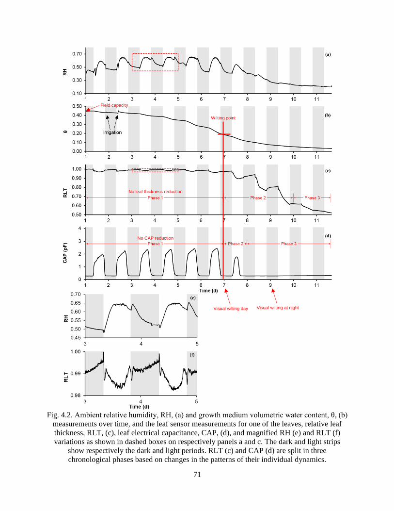
71
Fig. 4.2. Ambient relative humidity, RH, (a) and growth medium volumetric water content, θ, (b)
measurements over time, and the leaf sensor measurements for one of the leaves, relative leaf
thickness, RLT, (c), leaf electrical capacitance, CAP, (d), and magnified RH (e) and RLT (f)
variations as shown in dashed boxes on respectively panels a and c. The dark and light strips
show respectively the dark and light periods. RLT (c) and CAP (d) are split in three
chronological phases based on changes in the patterns of their individual dynamics.
No leaf thickness reduction
No CAP reduction
Wilting point
Visual wilting day Visual wilting at night
Field capacity

72
Fig. 4.3. Relative leaf thickness (RLT) variations of five tomato leaves other than that displayed
in Fig. 4.2-C. The dark and light strips show respectively the dark and light periods.

73
Fig. 4.4. Leaf electrical capacitance (CAP) variations of five tomato leaves other than that shown
in Fig. 4.2-D. The leaves of the panels match with the panel labels of Fig. 3. The dark and light
strips show respectively the dark and light periods.

74
Relative thickness
RLT dynamics (Fig. 4.2-C) showed small daily fluctuations, with slightly smaller values during
the light than dark periods during the first 6 days when θ decreased from 0.45 to 0.19
(approximately between the field capacity and wilting point). The night time RLT values
remained roughly constant on a daily basis, during this period. The daily variations increased
between day seven through ten. During this time, RLT decreased more during the light periods
and recovered less in the dark periods in comparison with the previous day. As a result, an
overall descending trend was observed in the RLT variations from day seven through ten, when
the stress level was greater. The daily RLT fluctuations diminished in the last two days of the
trial when θ was below 0.05.
Fig. 4.3 shows the graphs of RLT versus time for the leaves other than that shown in Fig. 4.2-C.
All the leaves showed small daily RLT variations during the first six days and the last two days.
Their daily RLT fluctuations increased from day seven to ten creating the same pattern as
discussed for Fig. 4.2-C.
The full-range of RLT variations from the beginning to the end of the trial varied from leaf to
leaf. Table 4.1 shows the initial leaf thickness and the minimum recorded RLT during the trial
for all the leaves. The initial leaf thickness and the minimum recorded RLT were strongly
correlated (p-value<0.01).
In addition, the displayed leaf in Fig. 4.3-E showed an overall slightly increasing trend during the
first four days.
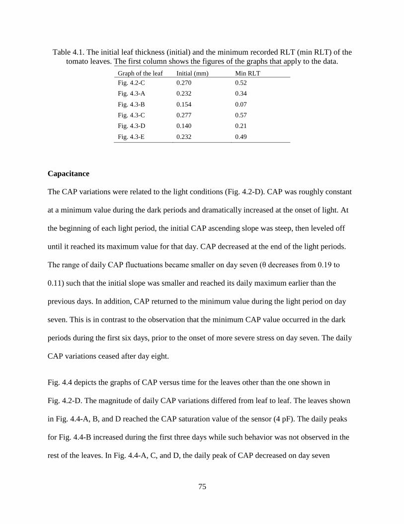
75
Table 4.1. The initial leaf thickness (initial) and the minimum recorded RLT (min RLT) of the
tomato leaves. The first column shows the figures of the graphs that apply to the data.
Graph of the leaf Initial (mm) Min RLT
Fig. 4.2-C 0.270 0.52
Fig. 4.3-A 0.232 0.34
Fig. 4.3-B 0.154 0.07
Fig. 4.3-C 0.277 0.57
Fig. 4.3-D 0.140 0.21
Fig. 4.3-E 0.232 0.49
Capacitance
The CAP variations were related to the light conditions (Fig. 4.2-D). CAP was roughly constant
at a minimum value during the dark periods and dramatically increased at the onset of light. At
the beginning of each light period, the initial CAP ascending slope was steep, then leveled off
until it reached its maximum value for that day. CAP decreased at the end of the light periods.
The range of daily CAP fluctuations became smaller on day seven (θ decreases from 0.19 to
0.11) such that the initial slope was smaller and reached its daily maximum earlier than the
previous days. In addition, CAP returned to the minimum value during the light period on day
seven. This is in contrast to the observation that the minimum CAP value occurred in the dark
periods during the first six days, prior to the onset of more severe stress on day seven. The daily
CAP variations ceased after day eight.
Fig. 4.4 depicts the graphs of CAP versus time for the leaves other than the one shown in
Fig. 4.2-D. The magnitude of daily CAP variations differed from leaf to leaf. The leaves shown
in Fig. 4.4-A, B, and D reached the CAP saturation value of the sensor (4 pF). The daily peaks
for Fig. 4.4-B increased during the first three days while such behavior was not observed in the
rest of the leaves. In Fig. 4.4-A, C, and D, the daily peak of CAP decreased on day seven
76
compared to the earlier days. In Fig. 4.4-B, the maximum value of CAP lasted for a shorter time
on day seven than on the previous day. Therefore, although CAP was saturated for this leaf
during a part of day seven, the early descending trend of CAP during the light period of day
seven indicates that the peak was smaller on this day than the previous day. However, the
smallest peak in Fig. 4.4-B occurred during the first day. In contrast with the rest of the leaves,
the daily peak of the leaf shown in Fig. 4.4-E did not decrease in day seven. However, the width
of the CAP peak decreased on this day, and the decline in CAP began before the light period
ended, similar to the CAP decline of the other leaves on this day. The maximum CAP in Fig. 4.4-
C showed a different behavior from other leaves during the first six days. The daily CAP
variations ceased for all the leaves from day eight onwards.
As mentioned above, the patterns of RLT and CAP daily variations could be distinguished
chronologically with three distinct phases. RLT variations could be split into the phases of (fig.
2c): (1) day one to seven (θ from 0.45 down to 0.19, from the field capacity to the wilting point
equivalently), (2) day seven to ten (θ from 0.19 down to 0.05), and (3) day ten to the end of the
experiment (θ below 0.05). The first phase for CAP occurred on the same days as the first phase
for RLT, but later phases differed. For CAP the phases were (fig. 2d): (1) day one to seven (θ
from 0.45 down to 0.19), (2) day seven to eight (θ from 0.19 down to 0.11), and (3) day eight to
the end of the experiment (θ below 0.11). Therefore, we refer to these three phases as phase 1, 2,
and 3.

77
Discussion
Leaf thickness
The daily RLT variations appeared to reflect the changes in transpiration rate. For instance, the
daily RH variations indicated that transpiration during the light periods increased the
atmospheric water content. Therefore, the coincidence of daily maximum RH and daily
minimum RLT may provide evidence of the negative impact of transpiration rate on RLT. The
negative effect of light and the transpiration rate on leaf thickness was reported by a number of
researchers (Búrquez, 1987; Rozema et al., 1987; Syvertsen & Levy, 1982). Light stimulates the
stomatal opening that results in increased transpiration rate and leaf water loss and decreased
RLT accordingly (Rozema et al., 1987). The daily RH variations indicate that transpiration
during the light periods increased atmospheric water content.
The differences in the daily RLT variations across phases 1 to 3 corresponded to the growth
medium available water content (Fig. 4.2). Volumetric water content, θ, was adequate in phase 1
such that the plant could meet the transpiration demand. In other words, the transpired water
from the leaf was replenished by water from the growth medium. Therefore, the daily leaf water
content variations, and accordingly the daily RLT variations, were small in phase 1.
The generally slightly smaller daily RLT minimums in phase 2 indicate a possible small
imbalance between the transpiration demand and water uptake. Such a behavior was also
observed by Seelig et al. (2011) who reported that the range of daily RLT variations increased
when water stress increased.
Large soil water tension causes a large hydraulic resistance between the soil and the plant that
results in a small water uptake rate (Kramer & Boyer, 1995). Considering that θ was below the

78
wilting point in phase 2, implying a large growth medium-to-plant hydraulic resistance, the
depleted leaf water content could not be replenished by water uptake during the period of high
evaporative demand resulting in decreased RLT. The small RLT increase during the dark periods
in phase 2 indicates a low water uptake rate when the evaporative demand was small. Every day
in phase 2, the daily minimum RLT in the light period and maximum RLT in the consecutive
dark period was lower than during the previous day, which implies that water stress was
developing in the leaf.
The RH variations could be an evidence of the relationship between RLT and the water stress
level. The large RH increase in the light periods implies a high transpiration rate in phase 1 due
to a small growth medium-plant-atmosphere hydraulic resistance. The decreased daily peaks of
RH during phase 2 appear to be signals of developing water stress. The concurrence of the
phases of RLT variations with those of RH variations appear as evidence of the relationship
between the pattern of RLT dynamics and the water stress level.
The above explanations hold true for all the leaves in this study. The leaves were exposed to the
same level of light exposure and belonged to the same plant. Therefore, the effect of water stress
on RLT was expected to be similar across all leaves.
Although the leaves shared the same pattern of RLT dynamics, the range of variations differed
between the leaves. The source of this variability could be the differences in the leaf tissue
elasticity. As Table 4.1 shows, the thicker leaves had the larger minimum recorded RLT during
the experiment. In other words, the percentage of the leaf thickness shrinkage was less in thicker
leaves, or better said, the tissue elasticity was negatively correlated with the leaf thickness. The
thicker leaves were possibly the older leaves with more lignin content in their cell wall and a

79
more rigid structure (Lambers et al., 2008; Patakas & Noitsakis, 1997; Sylvester, 2001). Another
possibility could be the history of the leaves during their growth prior to the initiation of the
experiment. The sun leaves have longer palisade cells and a ticker mesophyll than the shade
leaves (Taiz & Zeiger, 2006). Therefore, the thicker leaves would be the leaves that received
more light during the initial growth stage. Previous work suggests that leaves grown in light have
greater lignin content (Cabane et al., 2012; Gall et al., 2015; Syros et al., 2005), implying a more
rigid structure. Therefore, the strong correlation between the initial leaf thickness and the
minimum RLT could be explained by the lower bulk elasticity of the thicker leaves.
Leaf growth could possibly be the source of the observed RLT increase in the leaf shown in
Fig. 4.3-E. Leaf growth occurs in both lateral and thickness dimensions (Jones, 2004; Taiz &
Zeiger, 2006). This leaf thickness growth was absent in the other leaves.
Generally, the overall trend of the RLT variations reflected the pattern of the plant water stress
levels. Stress level is zero in a range of soil water content from field capacity down to a threshold
(Saseendran et al., 2008). After the threshold, stress level develops as soil water is further
depleted. The water stress level is constant at its maximum value below a certain level of soil
water content. The phases of the RLT variations showed a similar pattern. The slope of the
averaged RLT was close to zero in phase 1 that turned to a trend with a negative slope in phase
2. The slope of the overall RLT trend again changed to zero in phase 3. By applying the pattern
of water stress levels, the phases 1 to 3 could be interpreted as respectively the zero stress level,
the developing water stress stage, and the most severe water stress level. This explanation
suggests that the plant could tolerate growth medium water content from field capacity to about -
1.5 MPa matric potential (θ = 0.19) without observable symptoms of water stress. The
observation that no visible wilting occurred in phase 1 supports this interpretation.

80
These results suggest that changes in the maximum RLT during the dark periods or minimum
RLT in the light periods in comparison with the previous days can possibly be useful tools for
estimating the occurrence of water stress. A smaller RLT in a dark period compared to the
previous dark period would indicate the lack of the medium available water such that the plant
was not able to take up water and recoup the leaf turgor and RLT accordingly. In addition, a
smaller RLT during the light periods in comparison with the previous day could be interpreted as
the development of a water stress condition.
Seelig et al. (2011) reported that 10% RLT reductions of cowpea were within the range of daily
fluctuations so that they were not appropriate to trigger irrigation. Accordingly, they proposed
the RLT reduction thresholds of greater than 15% as triggers for irrigation. Our study showed
that the percent RLT reduction in phase 2 in response to a given θ reduction varied across the
leaves of the same plant. Therefore, selecting criteria as the indicators of a critical water stress
requires a strategy that takes the variability of the RLT dynamics into account.
Capacitance
The hypothesis that CAP was positively correlated with leaf water content would mean that CAP
variations should be directly related to plant water status. The effect of light is excluded in the
dark periods to determine the effect of dehydration alone. CAP during the early dark periods
(when the plant was well watered) should be greater than that of late dark periods (when the
medium water content was substantially depleted and the plant was wilted) if CAP was a
measure of water content. However, CAP in the dark periods was virtually constant throughout
the trial.
81
It seems, instead, that CAP was impacted by light. The onset of light caused a rapid increase in
CAP that then leveled off until a maximum was reached. The minimum CAP value was roughly
constant during the dark periods. CAP variations therefore seem to be a measure of leaf
photosynthetic activity instead of water content (Taiz & Zeiger, 2006).
The effect of light on CAP through photosynthesis may be explained by the effect of
photosynthesis on the leaf solute contents and its resultant dielectric properties. Changes in
solute contents of a solution can pronounce various effects on the solution’s dielectric constant
(Grimnes & Martinsen, 2008; Pethig, 1979). Generally, increasing the concentration of solutes in
an aqueous solution reduces the dielectric constant of the solution (Pethig, 1979; Wang &
Anderko, 2001). The magnitude of the solute effect depends on the nature of the solute and the
frequency of the dielectric measurement. However, the effect of ions on the dielectric properties
can be reversed in biological tissues. An applied electric field moves the ions in a tissue such that
a double layer of counterions will be built across the inner membranes resulting in increasing the
tissue capacitive effect (Grimnes & Martinsen, 2008). Therefore, an increase in the tissue ion
concentration increases the electrical capacitance.
Photosynthesis dynamically changes the concentration of the leaf solutes (Taiz & Zeiger, 2006).
For example, illumination causes the accumulation of protons in the thylakoid lumen and anions
in the stroma. Therefore, photosynthesis results in an ion charge gradient across the thylakoid
membrane that creates an electrical potential difference (Taiz & Zeiger, 2006). Such local
potential differences and the increased ion concentration could be the sources of the observed
CAP changes.
82
Based on this interpretation, the stomatal conductance is expected to have a significant effect on
CAP through its role in photosynthesis. Stomatal closure as a result of water stress reduces the
rate of CO2 intake that slows down the photosynthetic activity (Yokota & Takahara, 2006;
Chandler & Bartels, 1999; Taiz & Zeiger, 2006). Such behavior was observed in the CAP
dynamics. The amplitude of CAP decreased in day seven likely coinciding with partial stomatal
closure and reduced photosynthesis. Disappearance of the daily CAP fluctuations from day eight
onward could coincide with the absence of photosynthesis due to water stress.
The daily CAP peaks corresponded with the critical points in the RLT and RH dynamics such
that they would have emphasized the effect of stomatal conductance on CAP. The peaks of RH
occurred when CAP was at its maximum as well. In addition, the pattern of RH dynamics were
similar to those of CAP. Both showed large variations in phase 1, smaller variations on day
seven, and ceased thereafter. Reduced RH was reflective of a reduced transpiration rate because
of increased stomatal resistance. In addition, a critical point could be distinguished on the RLT
dynamics during the light periods. In phase 1, a minimum LT occurred during the light periods
where LT increased thereafter. In phase 2, this critical point turned into a moment that the rate of
the light time LT reduction decreased. A reduced stomatal conductance would explain these
changes in the RLT dynamics. A smaller stomatal conductance reduces the transpiration rate
(Taiz, 1984) that can potentially decrease the rate of LT reduction. Rozema et al. (1987) reported
a negative relationship between leaf thickness and stomatal conductance. Therefore, since the
mentioned critical points on the RH and RLT variations can be explained by changes in the
stomatal conductance, the concurrence of these critical points with the onset of the daily CAP
descending trend would suggest there is evidence that stomatal conductance and accordingly,
photosynthesis affected CAP.
83
Sinha & Tabib-Azar (2016) also reported a positive effect of illumination and a negative impact
of water stress on the electrical capacitance of Schefflera arboricola. They observed that the
capacitance increased in the daylight but the extent of the increment was dependent on the water
stress.
Afzal et al. (2010) reported a positive relationship between the sensor capacitance and the leaf
water content while the observations in this study did not follow a similar pattern. They used a
capacitive sensor composed of two parallel plates with a constant distance. The space between
the capacitive plates was occupied by the inserted leaf and an airspace. CAP was therefore a
composite of air and the leaf. As a result, the leaf thickness impacted the proportion of the space
between the capacitive plates occupied by the leaf and, in turn, the dielectric constant. Therefore,
the measured capacitance was probably affected by the leaf thickness. However, the different
species and measurement frequencies could also affect the results of these two studies. Afzal et
al. (2010) used corn, sorghum, common bean, and sunflower, while tomato was used in the
current study. The frequencies used in their study was 100 kHz and 1 MHz, but it was 32 kHz in
this study. In addition, Afzal et al. (2010) conducted their experiment on cut leaves in a lab
condition such that the effect of photosynthesis on the sensor capacitance was not considered.
The amplitude of CAP measurements varied across the leaves in this study (Fig. 4.2-D and
Fig. 4.4). This was probably a result of physiological differences between the leaves that affected
the photosynthetic capacity, such as stomatal density and chlorophyll density (Taiz & Zeiger,
2006).
For the leaf shown in Fig. 4.4-B, the increasing trend of daily CAP peak in the first three days
might be explained by recognizing an optimum available water content existed and that the plant

84
leaf was acclimating to the new environment (moving the plant from the greenhouse to the
growth chamber). Acclimation can result in improved photosynthetic activity (Taiz & Zeiger,
2006). However, the fluctuations in CAP during a portion of the light time period for the leaf
shown in Fig. 4.4-C remain unexplained.
This study therefore suggests that CAP can be a measure of photosynthetic activity, which in
turn can be employed to detect plant water (or other) stress(s). Indicators of stress based on CAP
variations could be a reduced maximum, a smaller area below the curve, and a short-lasting CAP
pulse. The effect of water stress was more pronounced on the CAP dynamics than the RLT
variations since it caused the complete cessation of CAP fluctuations from day eight. However,
stresses other than water deficit may reduce the photosynthesis and CAP in turn. For example,
pests and nutrition deficiencies can potentially reduce the photosynthetic activity (Ashraf &
Harris, 2013; Synková et al., 2006; Taiz & Zeiger, 2006) that may affect CAP.
The results showed that the plant did not show decreases of CAP, RLT, or signs of wilting from
the field capacity down to a matric potential of -1.5 MPa. Once the growth medium matric
potential decreased below this, however, these indicators were all evidence of plant stress.
The suggested explanation for CAP variations were that the solute contents resulting from
photosynthesis impacted readings. There are, of course, other factors that may affect the leaf
solute contents and thus may impact CAP dynamics. For example, soil salinity and fertilizers can
increase the leaf solute concentration (Ashraf & Harris, 2013; Liu et al., 2014; Taiz & Zeiger,
2006). However, the effect of such factors on the leaf solute contents and CAP accordingly is
possibly slow compared to the light effect. In addition, the behavior of CAP may be different for
various species. For example, the CAP variations may be affected by osmotic adjustment in

85
some species that accumulate solutes due to water stress (Yokota &Takahara, 2006; Farooq et
al., 2009; Taiz & Zeiger, 2006), a phenomenon that is absent in tomato (Rudich & Luchinsky,
1986).
Conclusion
Leaf thickness appeared to reflect the transpiration rate and water stress level. The range of leaf
thickness variations was small and consistent during a wide range of θ from field capacity to
wilting point. At that point leaf thickness decreased, first during the light period, with recovery
during the dark period. With increasing water stress level, RLT decreased more during the light
period and did not recover during the dark period. Therefore, the results suggest that RLT
reduction in comparison with previous days can be used to estimate plant water status during
daylight (when radiation is highest). CAP was strongly related to the light state that appeared to
reflect a strong relationship between photosynthesis and CAP. In addition, water stress reduced
the effect of light on CAP. The water stress could be distinguished from the decreased maximum
values of CAP during the light periods. Therefore, CAP could be an indirect measure of plant
water stress (or any other stress) through its effect on photosynthesis. Results may vary
depending on the sensor design and the measurement frequency as well as the plant species and
the environmental factors. Therefore, further studies are required to assess LT and CAP
variations versus water stress levels. However, the results of this study suggest that plant-based
sensors measuring RLT and CAP can be used to measure water stress directly on plants instead
of indirectly using soil matric potential, soil moisture content, or evapotranspiration models.
References
Afzal, A., Mousavi, S., & Khademi, M. (2010). Estimation of leaf moisture content by

86
measuring the capacitance. Journal of Agricultural Science Technology, 12, 339–346.
Ali, M. H. (2011). Practices of irrigation and on-farm water management: volume 2. Springer
(Vol. 2). New York: Springer.
Ashraf, M., & Harris, P. J. C. (2013). Photosynthesis under stressful environments: an overview.
Photosynthetica, 51(2), 163–190.
Baxter, L. K. (1996). Capacitive sensors: design and applications. John Wiley & Sons. New
York: John Wiley & Sons.
Búrquez, A. (1987). Leaf thickness and water deficit in plants: a tool for field studies. Journal of
Experimental Botany, 38(186), 109–114.
Cabane, M., Afif, D., & Hawkins, S. (2012). Lignins and abiotic stresses. In L. Jouanin & C.
Lapierre (Eds.), Advances in Botanical Research (1st ed., Vol. 61, pp. 219–262). Elsevier
Ltd.
Chandler, J., & Bartels, D. (1999). Plant desiccation. In H. R. Lerner (Ed.), Plant response to
environmental stresses: from phytohormones to genome reorganization (pp. 575–590). New
York: Marcel Dekker.
Cohen, Y., Alchanatis, V., Meron, M., Saranga, Y., & Tsipris, J. (2005). Estimation of leaf water
potential by thermal imagery and spatial analysis. Journal of Experimental Botany, 56(417),
1843–1852.
Dadshani, S., Kurakin, A., Amanov, S., Hein, B., Rongen, H., Cranstone, S., … Ballvora, A.
(2015). Non-invasive assessment of leaf water status using a dual-mode microwave

87
resonator. Plant Methods, 11(1), 8.
Damour, G., Simonneau, T., Cochard, H., & Urban, L. (2010). An overview of models of
stomatal conductance at the leaf level. Plant, Cell and Environment, 33(9), 1419–1438.
Evett, S. R., Heng, L. K., Moutonnet, P., & Nguyen, M. L. (Eds.). (2008). Field estimation of
soil water content: a practical guide to methods, instrumentation and sensor technology.
International Atomic Energy Agency.
Farahani, H., Wagiran, R., & Hamidon, M. (2014). Humidity sensors principle, mechanism, and
fabrication technologies: a comprehensive review. Sensors, 14(5), 7881–7939.
Farooq, M., Wahid, A., Kobayashi, N., Fujita, D., & Basra, S. M. A. (2009). Plant drought stress:
effects, mechanisms and management. Agronomy for Sustainable Development, 29(1), 185–
212.
Gall, H., Philippe, F., Domon, J.-M., Gillet, F., Pelloux, J., & Rayon, C. (2015). Cell wall
metabolism in response to abiotic stress. Plants, 4(1), 112–166.
Gente, R., Born, N., Voß, N., Sannemann, W., Léon, J., Koch, M., & Castro-Camus, E. (2013).
Determination of leaf water content from terahertz time-domain spectroscopic data. Journal
of Infrared, Millimeter, and Terahertz Waves, 34(3-4), 316–323.
Grimnes, S., & Martinsen, Ø. G. (2008). Bioimpedance and Bioelectricity Basics (2nd ed). New
York: Academic Press.
Honeywell staff. (2010). HIH-5030/5031 series: low voltage humidity sensors (datasheet).
Honeywell International Inc. Retrieved August 15, 2016, from
88
http://sensing.honeywell.com/index.php?ci_id=49692.
Jones, H. G. (2004). Irrigation scheduling: advantages and pitfalls of plant-based methods.
Journal of Experimental Botany, 55(407), 2427–36.
Jones, H. G. (2014). Plants and microclimate: a quantitative approach to environmental plant
physiology (3rd ed). Cambridge: Cambridge University Press.
Klute, A. (Ed.). (1986). Methods of soil analysis: part 1—physical and mineralogical methods. In
American Society of Agronomy, Soil Science Society of America (2nd ed.). Madison, WI.
Kramer, P. J., & Boyer, J. S. (1995). Water relations of plants and soils. San Diego: Academic
Press.
Lambers, H., Chapin, F. S., & Pons, T. L. (2008). Plant physiological ecology. New York:
Springer New York.
Liu, C.-W., Sung, Y., Chen, B.-C., & Lai, H.-Y. (2014). Effects of nitrogen fertilizers on the
growth and nitrate content of lettuce (Lactuca sativa L.). International Journal of
Environmental Research and Public Health, 11(4), 4427–4440.
Malone, M. (1993). Rapid inhibition of leaf growth by root cooling in wheat: kinetics and
mechanism. Journal of Experimental Botany, 44(268), 1663–1669.
Marenco, R. a., Antezana-Vera, S. a., & Nascimento, H. C. S. (2009). Relationship between
specific leaf area, leaf thickness, leaf water content and SPAD-502 readings in six
Amazonian tree species. Photosynthetica, 47(2), 184–190.
McBurney, T. (1992). The relationship between leaf thickness and plant water potential. Journal

89
of Experimental Botany, 43(248), 327–335.
Meidner, H. (1952). An instrument for the continuous determination of leaf thickness changes in
the field. Journal of Experimental Botany, 3(9), 319–325.
Patakas, A., & Noitsakis, B. (1997). Cell wall elasticity as a mechanism to maintain favorable
water relations during leaf ontogeny in grapevines. American Journal of Enology and
Viticulture, 48(3), 352–356.
Pethig, R. (1979). Dielectric and electronic properties of biological materials. Chichester,
England: Wiley.
Rozema, J., Arp, W., Diggelen, J., Kok, E., & Letschert, J. (1987). An ecophysiological
comparison of measurements of the diurnal rhythm of the leaf elongation and changes of the
leaf thickness of salt-resistant dicotyledonae and monocotyledonae. Journal of
Experimental Botany, 38(188), 442–453.
Rudich, J., & Luchinsky, U. (1986). Water economy. In J. G. Atherton & J. Rudich (Eds.), The
tomato crop: a scientific basis for improvement (pp. 335–367). London: Chapman and Hall.
Saseendran, S. A., Ahuja, L. R., Ma, L., Timlin, D., Stöckle, C. O., Boote, K. J., … Yu, Q.
(2008). Current water deficit stress simulations in selected agricultural system models. In L.
R. Ahuja, V. R. Reddy, S. A. Saseendran, & Q. Yu (Eds.), Response of crops to limited
water: understanding and modeling water stress effects on plant growth processes,
advances in agricultural systems modeling series 1 (pp. 1–37). American Society of
Agronomy, Crop Science Society of America, Soil Science Society of America.

90
Scoffoni, C., Vuong, C., Diep, S., Cochard, H., & Sack, L. (2014). Leaf shrinkage with
dehydration: coordination with hydraulic vulnerability and drought tolerance. Plant
Physiology, 164(4), 1772–1788.
Seelig, H. D., Stoner, R. J., & Linden, J. C. (2011). Irrigation control of cowpea plants using the
measurement of leaf thickness under greenhouse conditions. Irrigation Science, 30(4), 247–
257.
Sharon, Y., & Bravdo, B. (1996). Irrigation control of citrus according to the diurnal cycling of
leaf thickness. In Conference on Water & Irrigation, Tel Aviv, Israel (pp. 273–283).
Sinha, K., & Tabib-Azar, M. (2016). Effect of light and water on Schefflera plant electrical
properties. Journal of Scientific Research and Reports, 9(4), 1–11.
Sylvester, A. (2001). Leaf shape and anatomy as indicators of phase change in the grasses:
comparison of maize, rice, and bluegrass. American Journal of Botany, 88(12), 2157–2167.
Synková, H., Semorádová, Š., Schnablová, R., Müller, K., Pospíšilová, J., Ryšlavá, H., …
Čeřovská, N. (2006). Effects of biotic stress caused by Potato virus Y on photosynthesis in
ipt transgenic and control Nicotiana tabacum L. Plant Science, 171(5), 607–616.
Syros, T. D., Yupsanis, T. A., & Economou, A. S. (2005). Expression of peroxidases during
seedling growth in Ebenus cretica L. as affected by light and temperature treatments. Plant
Growth Regulation, 46(2), 143–151.
Syvertsen, J., & Levy, Y. (1982). Diurnal changes in citrus leaf thickness, leaf water potential
and leaf to air temperature difference. Journal of Experimental Botany, 33(135), 783–789.
91
Taiz, L. (1984). Regulation of cell wall mechanical properties. Annual Review of Plant
Physiology, 35, 585–657.
Taiz, L., & Zeiger, E. (2006). Plant physiology (4th ed.). Sunderland, MA: Sinauer Associates.
Vile, D., Garnier, E., Shipley, B., Laurent, G., Navas, M.-L., Roumet, C., … Wright, I. J. (2005).
Specific leaf area and dry matter content estimate thickness in laminar leaves. Annals of
Botany, 96(6), 1129–36.
Vilsack, T., & Reilly, J. T. (2014). 2012 census of agriculture: farm and ranch irrigation survey
(2013). United States Department of Agriculture, National Agricultural Statistics Service
(Vol. 3). United States Department of Agriculture, National Agricultural Statistics Service.
Retrieved August 15, 2016, from
https://www.agcensus.usda.gov/Publications/2012/Online_Resources/Farm_and_Ranch_Irri
gation_Survey/fris13.pdf.
Wang, P., & Anderko, a. (2001). Computation of dielectric constants of solvent mixtures and
electrolyte solutions. Fluid Phase Equilibria, 186(1-2), 103–122.
White, J. W., & Montes-R, C. (2005). Variation in parameters related to leaf thickness in
common bean (Phaseolus vulgaris L.). Field Crops Research, 91(1), 7–21.
Yokota, A. K., & Takahara, K. A. (2006). Water stress. In K. V. Madhavaro, A. S. Raghavendra,
& K. Janardhanreddy (Eds.), Physiology and molecular biology of stress tolerance in plants
(pp. 15–39). Dordrecht, Netherlands: Springer.
Zimmermann, D., Reuss, R., Westhoff, M., Gessner, P., Bauer, W., Bamberg, E., …

92
Zimmermann, U. (2008). A novel, non-invasive, online-monitoring, versatile and easy
plant-based probe for measuring leaf water status. Journal of Experimental Botany, 59(11).

93
Chapter 5: Leaf thickness and electrical capacitance to estimate plant water
status in a greenhouse condition
94
Leaf thickness and electrical capacitance to estimate plant water status in a
greenhouse condition
Abstract
The objective of this experiment was to determine the relationship of leaf thickness (LT) and
capacitance (CAP) with plant water stress levels under lesser-controlled conditions than in the
previous experiment. Eight tomato plants (Solanum lycopersicum) were grown in a controlled
greenhouse, four in pots filled with a potting mixture and the others in pots with a loamy mineral
soil. One leaf sensor was clipped on a leaf of each plant. Ambient temperature, relative humidity,
light intensity, growth medium volumetric water content (θ) for each pot, and LT and CAP for
each leaf sensor were measured at five-minute intervals. The irrigation regime was designed
based on observed visual wilting stages which reflected increased water stress over time. The
designated stress levels ranged from a well-watered condition for the first and second irrigations
to an extreme stress level for the sixth irrigation.
The difference between night and day LT values increased with water stress development. CAP
was roughly at a constant minimum value during the nights and rapidly increased as plants were
exposed to light. The maximum daily CAP values decreased as water stress increased.
The daily night- and noon-time LT and noon-time CAP were used as daily critical values, and
normalized by specific procedures to calculate their relative values. Piecewise linear regression
gave strong relationships of these normalized daily critical values of LT and CAP with θ.
The visual wilting water stress levels were correlated with θ, growth medium matric potential
(ψ), and the daily critical values of LT and CAP. The means of ψ were not significantly different

95
across the water stress levels. Soil volumetric water content could identify the early water stress
levels for the potting mixture. However, θ could not identify the water stress levels for the
mineral soil. In contrast, relative noon-time LT clearly identified all the water stress levels for
the potting mixture, and the early stress levels for the mineral soil. Relative night-time LT was
insensitive to early stresses, while it identified the severe water stress levels. Relative noon-time
CAP distinguished the mid-range stress levels. The results indicate that a transition from a stress
level to the next level could be discerned by at least one of the relative values of LT or CAP.
Therefore, in contrast to the soil moisture measurements, the combination of the relative values
of LT and CAP could provide a complete coverage for identification of each water stress level.
Keywords: plant-based method, leaf sensor, water stress, water content, water potential,
photosynthesis, irrigation timing.

96
Abbreviations and symbols
a The intercept of the piecewise linear model of daily critical relative leaf
thickness/capacitance versus growth medium volumetric water content for where
growth medium volumetric water content is equal or smaller than the breakpoint
b1 The slope of the piecewise linear model of daily critical relative leaf
thickness/capacitance versus growth medium volumetric water content for where
growth medium volumetric water content is greater than the breakpoint
b2 The slope of the piecewise linear model of daily critical relative leaf
thickness/capacitance versus growth medium volumetric water content for where
growth medium volumetric water content is equal or smaller than the breakpoint
BD Bulk density
c The breakpoint of the piecewise linear model of daily critical relative leaf
thickness/capacitance versus growth medium volumetric water content
CAP Leaf electrical capacitance (measured by the leaf sensor)
CAParea Area below the curve of capacitance-time
CAPirr,m The maximum recorded capacitance from the latest irrigation until the interested
capacitance measurement
CAPm Maximum recorded leaf electrical capacitance from the beginning of the
experiment until the interested capacitance measurement
CAPmax Maximum daily capacitance
Irrsum Cumulative effective irrigation
Ks Growth medium saturation hydraulic conductivity
LT Leaf thickness

97
LTm Maximum recorded leaf thickness from the beginning of the experiment until the
interested leaf thickness measurement
LTmax Daily maximum leaf thickness
LTmin Daily minimum leaf thickness
RCAP Capacitance normalized by the maximum recorded capacitance from the
beginning of the experiment until the interested capacitance measurement
RCAPirr,max Daily maximum capacitance normalized by the maximum recorded capacitance
from the latest irrigation until the interested capacitance measurement
RCAPmax Daily maximum capacitance normalized by the maximum recorded capacitance
from the beginning of the experiment until the interested capacitance
measurement
RH Atmospheric relative humidity
RLTmax Daily maximum leaf thickness normalized by the maximum recorded leaf
thickness from the beginning of the experiment until the interested leaf thickness
measurement
RLTmin Daily minimum leaf thickness normalized by the maximum recorded leaf
thickness from the beginning of the experiment until the interested leaf thickness
measurement
WUE Water use efficiency
θ Growth medium volumetric water content
θFC Growth medium volumetric water content at field capacity
θs Growth medium saturation volumetric water content
θwp Growth medium volumetric water content at the matric potential of -1500 kPa

98
ψ Growth medium matric potential
Introduction
Common methods to measure plant water status are either based on evapotranspiration models or
soil moisture/potential measurements (Vilsack & Reilly, 2014). However, soil water
content/potential and evapotranspiration rate are related to plant water balance through
complicated relationships (Damour et al., 2010; Jones, 2004, 2014; Kramer & Boyer, 1995;
Saseendran et al., 2008). For example, soil-plant hydraulic resistance is a function of soil texture,
salinity, and root geometry (Brady, 1990; Feddes & Raats, 2004; Vogel et al., 2016). Similarly,
plant-atmosphere conductance is a function of stomatal behavior and density, leaf geometry, and
environmental factors such as wind speed, light intensity, and temperature (Damour et al., 2010;
Jones, 2014). These factors make the soil-plant-atmosphere water relations heavily
parameterized and difficult to use for practical applications. On the other hand, reducing the
number of included parameters in models will increase the cumulative errors that result in
increased uncertainty of plant water status estimations. Increased uncertainty can potentially lead
to an inaccurate irrigation timing that can result in yield or water loss.
Plant-based methods can also be used to measure water status. The advantage of the plant-based
methods is that they by-pass the complicated soil-plant-atmosphere relationships to determine
plant water status (Jones, 2004; Kramer & Boyer, 1995). However, the majority of the plant-
based methods are not suitable for automatic monitoring systems, such as tissue weighing and
growth chamber techniques that are invasive to the plant, or porometer that are labor intensive
(Jones, 2004; Kramer & Boyer, 1995). Some researchers have used canopy thermal imaging as a
promising plant-based technique for automatic monitoring of plant water status (Cohen et al.,
99
2005; O’Shaughnessy & Evett, 2010). However, canopy temperature is also dependent on the
stomatal behavior and environmental factors, such as ambient temperature, wind speed, and light
intensity (Jones, 2014). As a consequence, thermal canopy sensing requires calibration (Jones,
2004).
Another promising method is leaf thickness (LT) measurements. For the first time, Bachmann
(1922) observed that leaves shrink by dehydration and swell by irrigation. Several researchers
reported strong positive correlations between leaf water content/potential and LT (Búrquez,
1987; Meidner, 1952; Neumann et al.,1974; Scoffoni et al., 2014). In addition, some studies
showed a negative association of LT with transpiration rate (Búrquez, 1987; Giuliani et al., 2013;
Rozema et al.,1987; Seelig et al., 2011). Leaf thickness was negatively associated with ambient
temperature and light intensity, while it was positively correlated with atmospheric relative
humidity (RH) (Búrquez, 1987; Rozema et al., 1987; Syvertsen & Levy, 1982). Therefore, leaf
thickness may be a suitable measure of plant water stress.
Because of the strong relationship between LT and leaf water content/potential, some researchers
have attempted to use LT measurements as a means for estimating plant water status. The early
instruments used for LT measurements were calipers and micrometers that were not suitable for
automatic measurements (Búrquez, 1987; Marenco et al., 2009; Meidner, 1952; White &
Montes-R, 2005). Some other researchers used linear variable distance transducers (LVDT) that
could be used in automatic systems (Dongsheng et al., 2007; Malone, 1993; McBurney, 1992;
Syvertsen & Levy, 1982; Vile et al., 2005). Rozema et al. (1987) developed a LT sensor by
employing a potentiometer to estimate leaf thickness. However, these instruments were bulky
and hard to use for practical applications.

100
Sharon and Bravdo (1996) designed a small leaf sensor using strain gauges. They evaluated their
sensor on grapefruit cv. Oroblanco (Citrus x paradisi Macfad) to improve irrigation water use
efficiency. They reported that the sensor-based treatments resulted in the highest water use
efficiency (WUE) compared to the preset irrigation schedule treatments. Seelig et al. (2011)
developed a small leaf sensor and assessed it on cowpea. In their study, the sensor-based
irrigation timing treatments saved 25-45% of irrigation water in comparison with the
prescheduled irrigation treatments.
These studies suggest LT measurements as a promising plant-based method for estimation of
plant water status and irrigation scheduling. However, some questions related to the
implementation of this method for practical applications remain unanswered. In an automatic
system, a quantified relationship is required for converting the LT variations to meaningful water
status levels. However, the earlier studies did not provide a quantitative guideline for detection of
critical plant water stress levels by LT variations. Although Seelig et al. (2011) introduced some
relative leaf thickness thresholds to trigger irrigation, these thresholds were determined
independent from the soil or plant measurements, such as plant water content/potential, soil
moisture measurements, visual wilting signs, or yield.
Since water has a large dielectric constant compared to most other materials in nature (Pethig,
1979), dielectric constant measurements have been used to estimate moisture content of various
materials, such as soil (Evett et al., 2008) and the atmosphere (Farahani et al., 2014). Leaf
dielectric constant could therefore be an alternative measure of leaf water content besides LT.
Afzal et al. (2010) developed a capacitive sensor with parallel capacitive plates and assessed it
on detached leaves of corn, sorghum, common bean, and sunflower at measurement frequencies

101
of 100 kHz and 1 MHz. They reported positive correlations between leaf water content and
capacitance. In addition, some other researchers studied the relationship between leaf electric
capacitance and plant water status using microwave measurement techniques (Dadshani et al.,
2015; Gente et al., 2013; Sinha & Tabib-Azar, 2016). They reported that water stress resulted in
changes in the measurement dynamics as signals of water stress. However, these sensors are not
suitable for practical automation applications because of the bulky structures and the complexity
of the methods.
In the previous experiment, the responses of LT and CAP to water stress were examined on a
tomato plant in highly controlled conditions. In that trial, LT and CAP dynamics were shown to
be sensitive to water stress. CAP was related to illumination when adequate water was available.
This unexpected result suggests that CAP reflects photosynthetic activity, and can reflect the
effect of water stress that limits photosynthesis.
The objective of the present study was to determine the relationship of LT and CAP with plant
water status determined by growth medium volumetric water content (θ) and visual wilting signs,
and assess the variability of these relationships across two different growth media.
Materials and methods
Leaf sensor
The leaf sensor used and data acquisition system are explained in Chapter 4.
Experimental design
Eight tomato plants variety Celebrity F1 (Solanum lycopersicum) were seeded in 7-lit pots. Four
pots were filled with a mineral soil and four others were filled with a potting mixture.

102
The plants were grown in a greenhouse with day/night ambient temperature of 27/18 °C and a
combination of natural and artificial light to produce a 12-hr photoperiod. The pots were
randomly placed in a line on a bench (Fig. 5.1). Prior to our experiment, no water stress was
applied to the plants by irrigating the pots to saturation every three days.
Fig. 5.1. The order of the pots according to their growth medium. The pots filled with potting
mixture and mineral soil are shown respectively by a square or a circular shape. The labels
indicate the pot numbers.
The experiment was conducted for 29 days, started 60 days after planting. During this 29 day
period, water was applied to obtain water stress based on signs of visual wilting. This way, well-
watered, moderate, severe, and extreme water stress levels were obtained by observing no visual
wilting, occurrence of a moderate wilting during day, observing wilting during night, and visual
wilting during two consecutive nights. These four levels of water stress were considered for the
first and second (for well-watered), third and fourth (for moderate), fifth (for severe), and sixth
(for extreme) irrigation events. Thereafter, the plants were not irrigated in order to observe the
effect of complete desiccation on LT and CAP.
LT, CAP, growth medium volumetric water content (θ), ambient light, RH, and temperature
were measured at 5-min intervals.
A leaf sensor was mounted on a randomly selected mature leaf per plant to monitor CAP and LT
(eight leaf sensors in total).

103
Temperature, light, and RH were measured by respectively a thermocouple, a light dependent
resistor, and an HIH-5030 humidity sensor (Honeywell, USA). These measurements were
collected by a DT85M data logger (DataTaker, Australia). The data logger was used to calibrate
the thermocouple. The RH sensor was calibrated by the equation provided in the product
datasheet. The light sensor was calibrated by fitting a regression model on the paired
measurements of the light sensor and a lux meter (LabNavigator, Forston Labs, USA).
Volumetric water content was measured by inserting a soil moisture sensor (EC5-H2O, Decagon
Devices, USA) at the center of each pot. To calibrate the sensors, the plants were cut from the
growth medium surface after the trial. The pots were watered to saturation and left to dehydrate.
From this process, a linear equation was fitted to the paired measurements of the sensor output
and θ to develop the calibration model. The volumetric water content was found by weighing the
pots, calculating the gravimetric water content and finally, converting it to θ using the medium
bulk density (Klute, 1986).
Growth medium physical properties
After the experiment, all the plants were cut at the medium surface and medium physical
properties were determined.
Bulk density (BD) was calculated as follows:
BD =oven dried weight of the pot – empty pot weight
volume of the pot occupied by the growth medium (4)
Volumetric water content at field capacity (θFC) was approximated based on the maximum stable
θ after the first irrigation during the experiment (after draining the gravitational water). To find
the saturation volumetric water content (θs), the pots were placed in a tub and gradually filled
104
with water to the medium surface. The level of water increased in three steps with 24-hr
intervals. During this process, the tub was enclosed to limit the evaporation. When water was at
the medium surface for 48 hr, three samples were taken from the medium surface to measure the
wet weights. Then, samples were placed in an oven with the temperature of 105 °C for 48 hr to
calculate θs. To obtain the volumetric water content of the growth medium at the matric potential
(ψ) of -1 kPa, the level of water in the tub was decreased to 10 cm below the medium surface.
After 48 hr, three samples were taken from the medium surface to find θ.
Retention curves of the media were constructed by combining θs, θ at ψ = -1 kPa, paired
measurements of θ-ψ collected by tensiometers, and the data collected by the pressure plate
extractor method. A tensiometer was used for the wet parts of the retention curves, from field
capacity to ψ = -30 kPa for the potting mixture, and to ψ = -80 kPa for the mineral soil. A soil
moisture sensor and a tensiometer were inserted into each pot to collect θ-ψ measurements from
field capacity down to the minimum suction at which the tensiometer worked properly.
The pressure plate extractor method was used at the drier parts of the retention curve (Klute,
1986). Briefly, three samples were collected by 2.5 cm high × 5 cm diameter rings for each
pressure within the pots. The bottom of samples was covered with a cheese-cloth and placed on
the pressure plates. The samples and pressure plates were wetted from below and soaked in
distilled water for 24 hr. Then, the pressure plates and the samples were moved to the pressure
extractors and subject to the predetermined pressures. The samples were kept under the pressure
until the water out flux ceased. This process took four to ten days. The applied pressures were
1500 kPa for the mineral soil, and 70, 300, and 1500 kPa for the potting mixture.

105
The retention curves were created using RETC software, version 6.02, based on the Van
Genuchten model as follows (Radcliffe & Šimunek, 2010):
θ(ψ) = θr +θs − θr
[1 + (α|ψ|)n]1−1 n⁄ (5)
where, θ(ψ) is the volumetric water content (θ) at the growth medium matric potential of ψ, θr is
the residual θ, θs is the saturation θ, and α and n are the model parameters.
A cylindrical core sample (9 cm diameter × 12 cm height) was taken from each pot and the
growth medium saturation hydraulic conductivity (Ks) was measured by the constant head
method (Klute, 1986). The mineral soil texture was determined by the hydrometer method with
four replications (Klute, 1986).
Plant dry mass, yield, and water use efficiency
At the end of the experiment, the fruits of each plant were weighed as the fresh yield weight and
the plants were cut from the medium surface and dried in an oven (70°C for 48 hr) to measure
the plant dry mass.
The amount of water applied at each irrigation was determined. To determine it, for each
irrigation event, the difference in θ before and after the irrigation event was calculated. Through
this process, the volumetric water content after the irrigation was determined based on the
maximum stable θ following the irrigation and after the gravitational water had drained, and this
value was subtracted by θ at the irrigation time (minimum θ before the irrigation). The calculated
difference was multiplied by the volume of the pot to obtain the amount of applied water that the
growth medium could hold (here called effective irrigation). Cumulative effective irrigation
(Irrsum) was calculated as the sum of the effective irrigations for all the irrigation events within
106
the pots. Finally, the fresh yield was divided by Irrsum to find water use efficiency (WUE) for
each plant.
Statistical analysis
Minitab 16 was used for linear regression and correlation analysis. The piecewise linear
equations were fitted by the model procedure of SAS 9.4 based on the method explained by
Ryan and Porth (2007). The following equation shows the applied parametric piecewise model:
y = { 𝑎 + 𝑐(𝑏2 − 𝑏1) + 𝑏1θ, θ > 𝑐
𝑎 + 𝑏2θ, θ ≤ 𝑐 (6)
where, y is the response, θ is growth medium water content as the independent variable, c is the
breakpoint, a is the intercept for θ≤c, b1 is the line slope for θ>c, and b2 is the line slope for θ ≤c.
Results and discussion
Growth medium physical properties
Table 5.1 and Table 5.2 show the physical properties of the growth media by pot and medium.
Except for ѱ at θFC, the analysis of variance showed that all the physical properties significantly
varied by growth medium (p-value<0.05). Bulk density of the mineral soil was about seven
times that of the potting mixture, while Ks of the potting mixture was ten times greater than that
of the mineral soil. Subtracting θwp from θFC indicates that the potting mixture had a larger
available water holding capacity.

107
Table 5.1. Physical properties of the growth media by pots, where BD is the bulk density, Ks is
the saturation hydraulic conductivity, θs is the saturation volumetric water content, θFC is the
volumetric water content at field capacity, θwp is the volumetric water content at the water
potential of -1500 kPa. Pot
number Medium BD (g cm-3) Ks (cm day-1) θs θwp θFC ψ (kPa) at θFC
1 Potting 0.15 2799 0.90 0.20 0.66 -2
2 Mineral 1.23 256 0.70 0.18 0.44 -11
3 Potting 0.15 2447 0.91 0.18 0.58 -2
4 Mineral 1.01 304 0.68 0.17 0.45 -2
5 Potting 0.16 2842 0.90 0.20 0.54 -3
6 Potting 0.14 2521 0.90 0.21 0.68 -2
7 Mineral 1.06 207 0.59 0.15 0.43 -11
8 Mineral 1.11 210 0.68 0.17 0.40 -2
Table 5.2. Physical properties of the growth media (average values), where BD is the bulk
density, Ks is the saturation hydraulic conductivity, θs is the saturation volumetric water content,
θwp is the volumetric water content at the water potential of -1500 kPa.
Medium BD (g cm-3) Ks (cm day-1) θs θwp θFC
Potting 0.15 2652 0.90 0.21 0.62
Mineral 1.10 244 0.66 0.17 0.43
The mineral soil particle analysis showed that its texture was loam, composed of 47% sand, 45%
silt, and 8% clay. The information about the retention curves are provided in Appendix A.
Plant and environmental measurements
Table 5.3 and Table 5.4 display plant dry mass, fresh yield, and WUE respectively by pot and
medium. The analysis of variance showed that fresh yield and WUE significantly varied by
growth medium (p-value<0.05). Higher fertility of the potting mixture with a high organic matter
may explain the better yield and WUE of the plants grown in the potting mixture compared to
those in the mineral soil (Taiz & Zeiger, 2006).
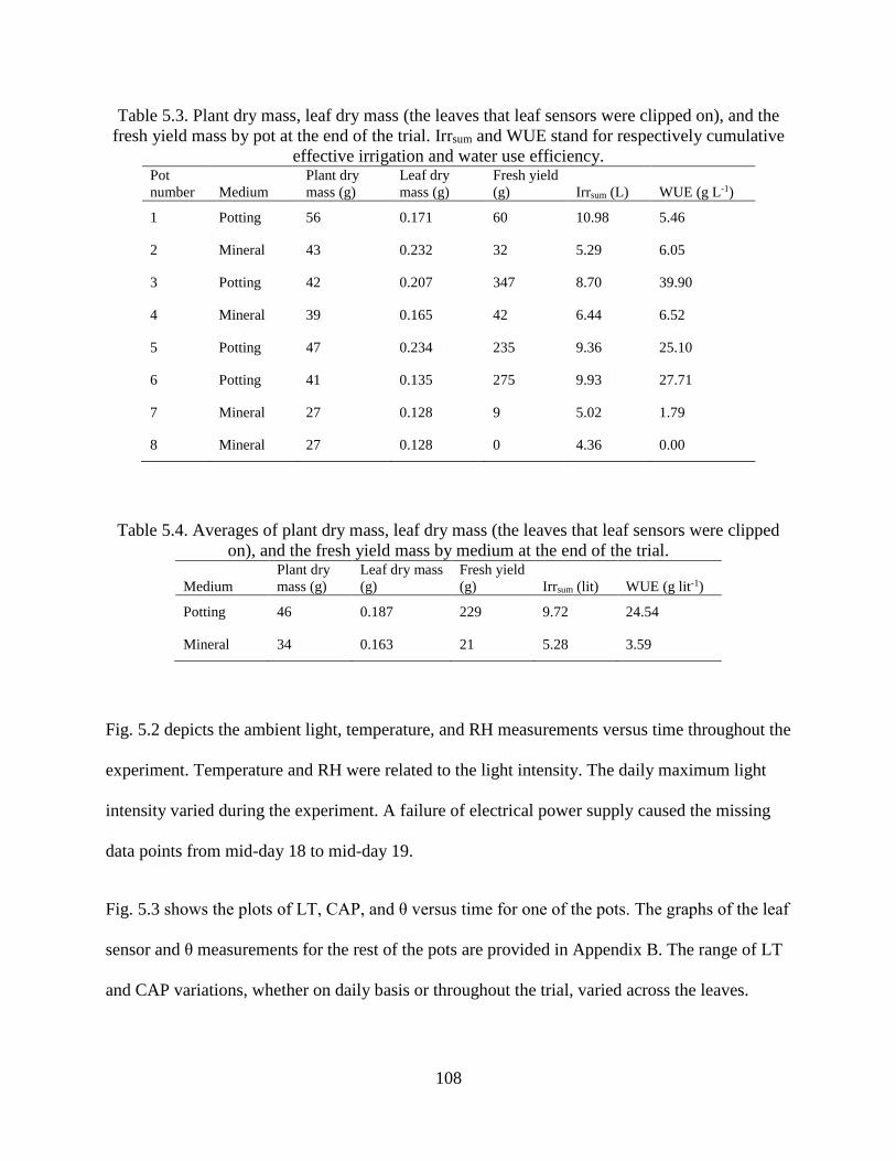
108
Table 5.3. Plant dry mass, leaf dry mass (the leaves that leaf sensors were clipped on), and the
fresh yield mass by pot at the end of the trial. Irrsum and WUE stand for respectively cumulative
effective irrigation and water use efficiency. Pot
number Medium
Plant dry
mass (g)
Leaf dry
mass (g)
Fresh yield
(g) Irrsum (L) WUE (g L-1)
1 Potting 56 0.171 60 10.98 5.46
2 Mineral 43 0.232 32 5.29 6.05
3 Potting 42 0.207 347 8.70 39.90
4 Mineral 39 0.165 42 6.44 6.52
5 Potting 47 0.234 235 9.36 25.10
6 Potting 41 0.135 275 9.93 27.71
7 Mineral 27 0.128 9 5.02 1.79
8 Mineral 27 0.128 0 4.36 0.00
Table 5.4. Averages of plant dry mass, leaf dry mass (the leaves that leaf sensors were clipped
on), and the fresh yield mass by medium at the end of the trial.
Medium
Plant dry
mass (g)
Leaf dry mass
(g)
Fresh yield
(g) Irrsum (lit) WUE (g lit-1)
Potting 46 0.187 229 9.72 24.54
Mineral 34 0.163 21 5.28 3.59
Fig. 5.2 depicts the ambient light, temperature, and RH measurements versus time throughout the
experiment. Temperature and RH were related to the light intensity. The daily maximum light
intensity varied during the experiment. A failure of electrical power supply caused the missing
data points from mid-day 18 to mid-day 19.
Fig. 5.3 shows the plots of LT, CAP, and θ versus time for one of the pots. The graphs of the leaf
sensor and θ measurements for the rest of the pots are provided in Appendix B. The range of LT
and CAP variations, whether on daily basis or throughout the trial, varied across the leaves.

109
Generally, LT was smaller during the days than nights. A smaller θ was associated with larger
daily LT variations. The night-time and noon-time LT decreased with a smaller θ. LT of some
plants showed an overall growth trend during the first half of the experiment. During the first
irrigation cycle (from the beginning of the experiment to day 6), LT showed small daily
variations with a consistent pattern. The last day of the second and third irrigation cycles showed
larger daily variations. This range of daily fluctuations increased on the last day of the later
irrigation cycles. The daily LT variations decreased from day 26 to the end of the experiment.
The observed associations between LT variations and light and θ can be explained by changes in
the leaf water balance through transpiration and water uptake. Earlier studies reported a negative
relationship between LT and transpiration rate (Búrquez, 1987; Giuliani et al., 2013; Rozema et
al., 1987). Seelig et al.(2011) observed that the range of daily LT fluctuations increased at
smaller θ values.
In our study, the range of daily LT variations was associated with the applied water stress levels
across the irrigation cycles, suggesting the night-time and noon-time LT values may be
promising measures of plant water status.

110
Fig. 5.2. The environmental measurements versus time: ambient temperature (A), light (B), and relative humidity (C).

111
Fig. 5.3. The leaf sensor measurements and the growth medium volumetric water (θ) for one of the pots filled with potting mixture
(pot 1) versus time: leaf thickness, LT (A), electrical capacitance, CAP (B), and θ (C).
112
CAP was strongly associated with light exposure. CAP was roughly constant at a minimum
value during the nights and rapidly increased when exposed to light. Generally, the daily
maximum CAP (CAPmax) was larger on the days with a greater light intensity. In addition, a
small θ was associated with a small CAPmax such that daily CAP variations ceased during the last
three days of the experiment. Sinha and Tabib-Azar (2016) designed a 10 GHz microwave
sensor and assessed it in response to the water status of Schefflera arboricola. They observed
that the sensor capacitance was positively associated with light and negatively with water stress.
Because of the large dielectric constant of water (Pethig, 1979), our original hypothesis was that
there would be a positive correlation between leaf water content and CAP. If this hypothesis was
true, CAP should be positively correlated with θ during the nights (considering just nights to
reduce the effect of light). However, such a behavior was not observed; CAP was roughly
constant regardless of θ during the nights.
In contrast, it appears that the CAP variations may have been related to changes in the leaf solute
contents. Photosynthesis increases the solute contents (Taiz & Zeiger, 2006) such that it can
potentially affect the electrical capacitance of the tissue. Generally, an increase in the solute
concentration of aqueous solutions decreases the dielectric constant of the solution (Pethig, 1979;
Wang & Anderko, 2001). However, in biological tissues, an electric field applied on the tissue
polarizes the ion contents across the membranes that creates local electrical potential gradients,
that increases the electrical capacity of the tissue (Grimnes & Martinsen, 2008). Similarly,
photosynthesis causes the accumulation of anions in the stroma and protons in the lumen of
thylakoid that makes a potential gradient across the thylakoid membrane (Taiz & Zeiger, 2006).
Therefore, result of such local electrical gradients can potentially increase the electrical
capacitance of the tissue.

113
The effect of θ on CAP can therefore be explained as an indirect effect of water stress on
photosynthesis. Plants regulate the stomatal conductance by experiencing water stress to
minimize the transpiration rate to save water, which results in a reduced CO2 intake and
photosynthesis (Yokota & Takahara, 2006; Chandler & Bartels, 1999; Taiz & Zeiger, 2006).
Therefore, decreased θ would reduce the photosynthetic activity and CAP accordingly.
In this interpretation, the hypothesized effect of photosynthesis on CAP was explained by the
effect of photosynthesis on the leaf solute content variations. However, the effects of solute and
ionic contents vary for different measurement frequencies (Grimnes & Martinsen, 2008; Pethig,
1979). The effects of solutes can be amplified at smaller frequencies (Grimnes & Martinsen,
2008; Ishai, Talary, Caduff, Levy, & Feldman, 2013; Pethig, 1979; Schwan, 1992; Yoon, 2011);
(our sensor operated at a frequency of 32kHz). Therefore, the observed effects on the
measurements can be different for various frequencies. For example, the effect of photosynthesis
may be reduced at higher frequencies such that the effect of water content variations may be the
dominant effect. However, the smaller CAP values and higher noise gains associated with higher
frequencies would be a concern (Afzal et al., 2010).
Analyses of leaf thickness and capacitance variations
Instead of modeling all the LT and CAP variations, the critical points of the curves were
extracted and analyzed. This method has two major advantages for automatic systems. It
decreases the number of data points, thereby decreasing computational cost. In addition, the
system will only need to collect data at certain moments when approximate critical values are
expected, for example, at some data points around 1:00 pm and 3:00 am when respectively the
approximate daily maximum and minimum light intensity and temperature (maximum and
minimum transpiration rates) are expected. Therefore, the power consumption of the

114
measurement device will be significantly reduced from that required for a system that collects
data with short intervals. This can be an essential advantage for a battery-operated device.
As mentioned earlier, the dynamics of LT and CAP had daily fluctuations with distinct daily
minimum and maximum values.
Daily maximum and minimum LT (LTmax and LTmin) were observed respectively at night and
close to time. This reflects the negative correlation of LT and transpiration rate reported by other
researchers (Búrquez, 1987; Giuliani et al., 2013; Rozema et al., 1987). Therefore, LTmax and
LTmin can be considered as respectively the highest and lowest leaf turgor during night and day.
Similarly, the daily minimum and maximum CAP occurred at respectively night and day.
However, the minimum CAP did not provide interesting information since it was roughly
constant during the nights throughout the experiment. On the other hand, the daily maximum
CAP (CAPmax) coincided with the maximum light intensity, which was approximately at noon.
Assuming that CAP was a measure of photosynthetic activity, analysis of the effect of water
stress on CAPmax could be interpreted as the impact of water stress on the noon-time
photosynthetic activity.
The following section, the relationships between the daily minimum and maximum values of LT
and CAP versus θ and then, versus the visual water stress levels are presented.
Leaf thickness versus growth medium water content
The daily maximum and minimum LT values (LTmax and LTmin) were extracted from the
measurements as the daily critical values to investigate their relationships with θ.
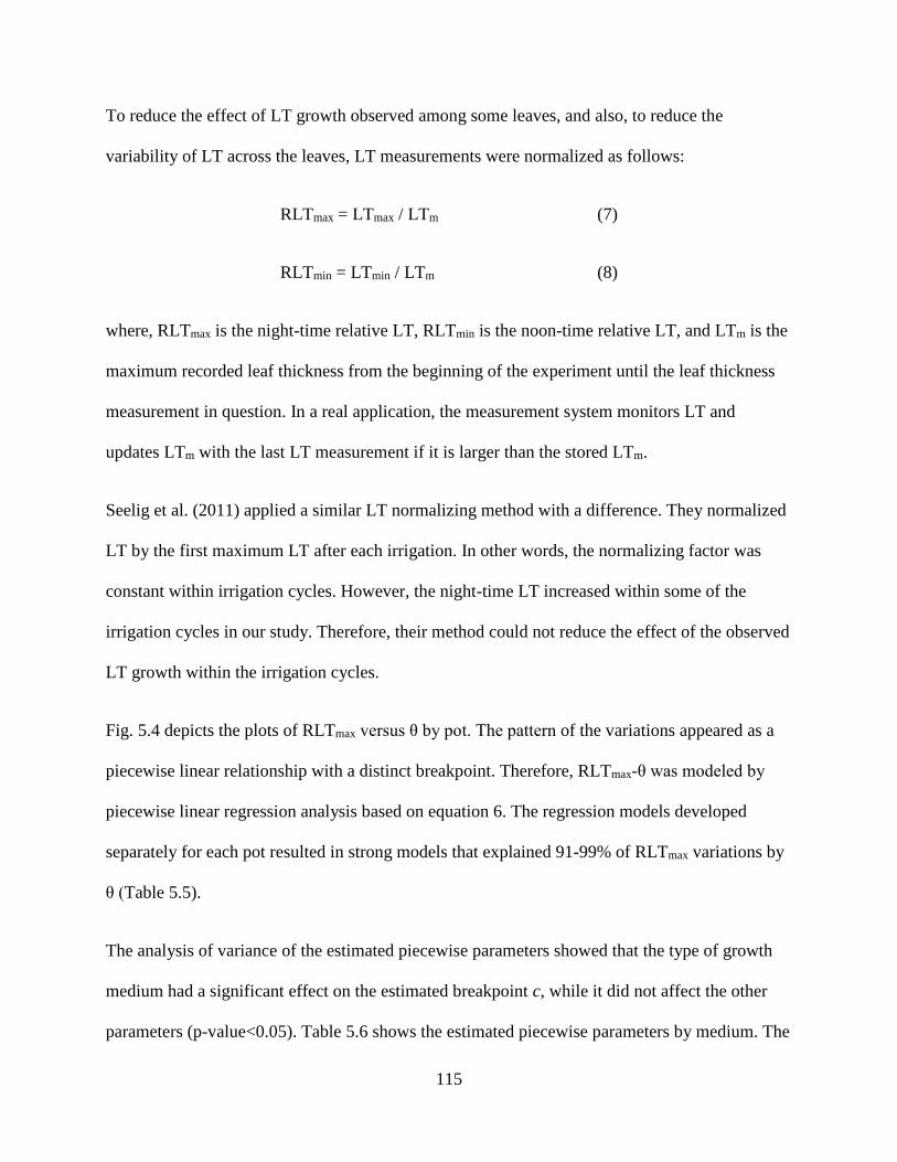
115
To reduce the effect of LT growth observed among some leaves, and also, to reduce the
variability of LT across the leaves, LT measurements were normalized as follows:
RLTmax = LTmax / LTm (7)
RLTmin = LTmin / LTm (8)
where, RLTmax is the night-time relative LT, RLTmin is the noon-time relative LT, and LTm is the
maximum recorded leaf thickness from the beginning of the experiment until the leaf thickness
measurement in question. In a real application, the measurement system monitors LT and
updates LTm with the last LT measurement if it is larger than the stored LTm.
Seelig et al. (2011) applied a similar LT normalizing method with a difference. They normalized
LT by the first maximum LT after each irrigation. In other words, the normalizing factor was
constant within irrigation cycles. However, the night-time LT increased within some of the
irrigation cycles in our study. Therefore, their method could not reduce the effect of the observed
LT growth within the irrigation cycles.
Fig. 5.4 depicts the plots of RLTmax versus θ by pot. The pattern of the variations appeared as a
piecewise linear relationship with a distinct breakpoint. Therefore, RLTmax-θ was modeled by
piecewise linear regression analysis based on equation 6. The regression models developed
separately for each pot resulted in strong models that explained 91-99% of RLTmax variations by
θ (Table 5.5).
The analysis of variance of the estimated piecewise parameters showed that the type of growth
medium had a significant effect on the estimated breakpoint c, while it did not affect the other
parameters (p-value<0.05). Table 5.6 shows the estimated piecewise parameters by medium. The
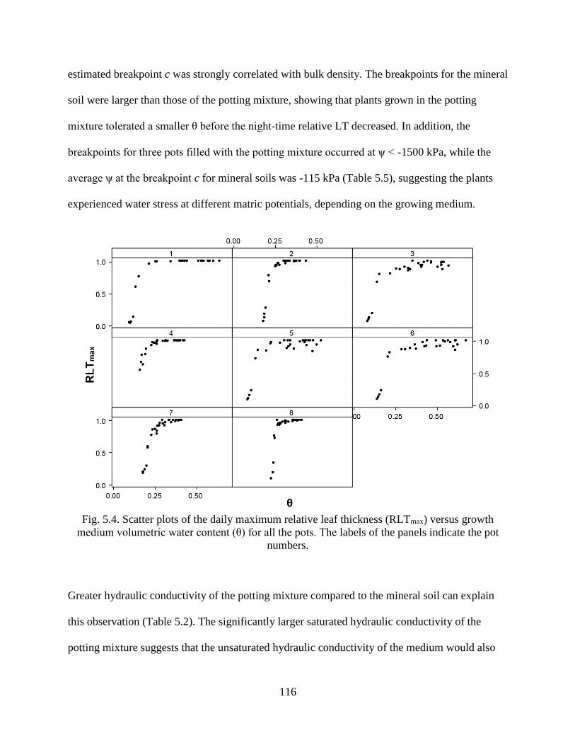
116
estimated breakpoint c was strongly correlated with bulk density. The breakpoints for the mineral
soil were larger than those of the potting mixture, showing that plants grown in the potting
mixture tolerated a smaller θ before the night-time relative LT decreased. In addition, the
breakpoints for three pots filled with the potting mixture occurred at ψ < -1500 kPa, while the
average ψ at the breakpoint c for mineral soils was -115 kPa (Table 5.5), suggesting the plants
experienced water stress at different matric potentials, depending on the growing medium.
Fig. 5.4. Scatter plots of the daily maximum relative leaf thickness (RLTmax) versus growth
medium volumetric water content (θ) for all the pots. The labels of the panels indicate the pot
numbers.
Greater hydraulic conductivity of the potting mixture compared to the mineral soil can explain
this observation (Table 5.2). The significantly larger saturated hydraulic conductivity of the
potting mixture suggests that the unsaturated hydraulic conductivity of the medium would also

117
also be larger. Generally, the medium with higher organic matter content has better aggregation
and higher porosity, which results in a better medium hydraulic conductivity (Brady, 1990;
Eusufzai & Fujii, 2012; Nemes, Rawls, & Pachepsky, 2005). Therefore, the critical hydraulic
conductivity to limit the water uptake and reduce the night-time LT was expected to occur at a
smaller θ for the potting mixture with a higher organic matter compared to the mineral soil.
Table 5.7 displays the estimated piecewise parameters of RLTmax-θ for all the pots in a single
equation.
Table 5.5. The estimated piecewise linear model parameters of daily maximum relative leaf
thickness (RLTmax) versus growth medium volumetric water content (θ) by pot, where, c is the
breakpoint, a is the intercept for where θ≤c, and b1 and b2 are the slopes for where respectively
θ>c and θ≤c. Pot
number a b1 c b2
R2 of the
model RLTmax at c ψ (kPa) at c
1 -1.455 0.054 0.171 14.25 0.98 0.98 <-1500
2 -3.468 0.403 0.228 19.30 0.99 0.94 -309
3 -0.889 0.301 0.158 11.03 0.97 0.85 <-1500
4 -0.232 0.178 0.233 5.16 0.91 0.97 -29
5 -1.108 0.147 0.154 13.21 0.96 0.92 <-1500
6 -1.385 0.241 0.221 10.25 0.97 0.88 -30
7 -2.114 0.904 0.238 12.53 0.99 0.87 -99
8 -6.952 0.360 0.259 30.48 0.95 0.95 -22
Table 5.6. The estimated piecewise linear model parameters of daily maximum relative leaf
thickness (RLTmax) versus growth medium volumetric water content (θ) by growth medium,
where, c is the breakpoint, a is the intercept for where θ≤c, and b1 and b2 are the slopes for where
respectively θ>c and θ≤c.
Medium a b1 c b2
R2 of the
model RLTmax at c
Mineral -0.688 0.215 0.282 5.90 0.64 0.97
Potting -0.484 0.140 0.223 6.33 0.87 0.923

118
Table 5.7. The estimated piecewise linear model parameters of daily maximum relative leaf
thickness (RLTmax) versus growth medium volumetric water content (θ) for all the pots, where, c
is the breakpoint, a is the intercept for where θ≤c, and b1 and b2 are the slopes for where
respectively θ>c and θ≤c.
a b1 c b2
R2 of the
model RLTmax at c
-0.295 0.020 0.285 4.44 0.73 0.97
The breakpoint c represents the volumetric water content at which the rate of decrease of the
night-time LT versus θ changed significantly. The breakpoint c reflected therefore the critical
water content at which the plants started to experience significant turgor loss at night. However,
turgor loss at night occurs under severe water stress. Therefore, it suggests that night-time LT
would be a suitable signal for late, but not early detection of water stress.
Fig. 5.5 depicts the plots of RLTmin versus θ, implying a piecewise linear relationship. Therefore,
equation 6 was used to model the RLTmin - θ relationship. Table 5.8 shows the estimated
piecewise parameters for RLTmin versus θ by pot. The models explained 68-92% of RLTmin
variations. The analysis of variance showed that the type of growth medium did not have a
significant effect on model parameters (p-value<0.05). The R2 of the model developed for all the
pots was 72% (Table 5.9).
Table 5.8 shows that the breakpoints occurred at larger θ and ѱ values compared to those of
RLTmax, showing that noon-time LT responded to water stress at a higher θ compared to night-
time LT. Therefore, RLTmin appeared as an earlier water stress signal compared to RLTmax.
Table 5.8 shows that RLTmin at the estimated breakpoints were equal to or smaller than 0.85.
This result is in agreement with the study of Seelig et al. (2011) on LT dynamics of cowpea.
They suggested RLTmin≤0.85 as the irrigation timing thresholds since the larger values may fall
into the normal daily LT fluctuations.

119
Fig. 5.5. Scatter plots of the daily minimum relative leaf thickness (RLTmin) versus growth
medium volumetric water content (θ) for all the pots. The method of RLTmin calculation is
presented in the text. The labels of the panels indicate the pot numbers.
Table 5.8. The estimated piecewise linear model parameters of daily minimum relative leaf
thickness (RLTmin) versus growth medium volumetric water content (θ) by pot, where, c is the
breakpoint, a is the intercept for where θ≤c, and b1 and b2 are the slopes for where respectively
θ>c and θ≤c. Pot
number a b1 c b2
R2 of the
model RLTmin at c ψ (kPa) at c
1 -0.320 0.195 0.273 3.97 0.90 0.76 -12
2 -1.177 0.296 0.295 6.84 0.89 0.84 -75
3 -0.143 -0.114 0.328 2.95 0.92 0.82 -5
4 0.027 0.304 0.281 2.93 0.84 0.85 -12
5 -0.247 0.165 0.233 3.96 0.90 0.67 -20
6 -0.249 0.065 0.383 2.61 0.90 0.75 -6
7 -1.813 0.632 0.241 10.36 0.87 0.68 -94
8 -2.462 1.845 0.274 11.80 0.68 0.77 -16

120
Table 5.9. The estimated piecewise linear model parameters of daily minimum relative leaf
thickness (RLTmin) versus growth medium volumetric water content (θ) for all the pots, where, c
is the breakpoint, a is the intercept for where θ≤c, and b1 and b2 are the slopes for where
respectively θ>c and θ≤c.
a b1 c b2
R2 of the
model RLTmin at c
-0.253 -0.147 0.317 3.38 0.72 0.82
Capacitance versus growth medium water content
The range of daily CAP fluctuations varied across the leaves. Therefore, the same approach for
normalizing leaf thickness was applied for CAPmax:
RCAPmax = CAPmax / CAPm (9)
where, CAPmax is the daily maximum CAP (the noon-time CAP), CAPm is the maximum
recorded CAP from the beginning until the respective measurement, and RCAPmax is the relative
daily maximum CAP. In a real application, the measurement system monitors CAP and updates
CAPm with the last CAP measurement if it is larger than the stored CAPm.
The relationship of RCAPmax and θ was analyzed. Fig. 5.6 shows the scatter plots of RCAPmax-θ
by pot. The plots of RCAPmax-θ appeared to have a piecewise linear relationship. Therefore, the
parametric equation 6 was applied to RCAPmax-θ considering b1≥0 as a boundary limit of the
model. This limit was considered since estimated b1 for some of the pots were negative with p-
value<0.05. However, assuming that CAP is a measure of photosynthesis, a negative effect of θ
on photosynthesis and RCAPmax in turn is not expected. It is worth mentioning that removing the
boundary limit did not improve the models.
Table 5.10 and Table 5.11 present the estimated piecewise parameters respectively by pot and all
the pots in one model. The models estimated by pots explained 56-95% of RCAPmax variations.
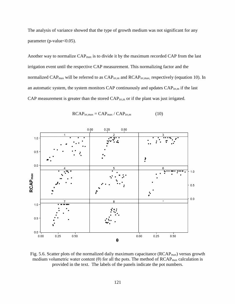
121
The analysis of variance showed that the type of growth medium was not significant for any
parameter (p-value<0.05).
Another way to normalize CAPmax is to divide it by the maximum recorded CAP from the last
irrigation event until the respective CAP measurement. This normalizing factor and the
normalized CAPmax will be referred to as CAPirr,m and RCAPirr,max, respectively (equation 10). In
an automatic system, the system monitors CAP continuously and updates CAPirr,m if the last
CAP measurement is greater than the stored CAPirr,m or if the plant was just irrigated.
RCAPirr,max = CAPmax / CAPirr,m (10)
Fig. 5.6. Scatter plots of the normalized daily maximum capacitance (RCAPmax) versus growth
medium volumetric water content (θ) for all the pots. The method of RCAPmax calculation is
provided in the text. The labels of the panels indicate the pot numbers.
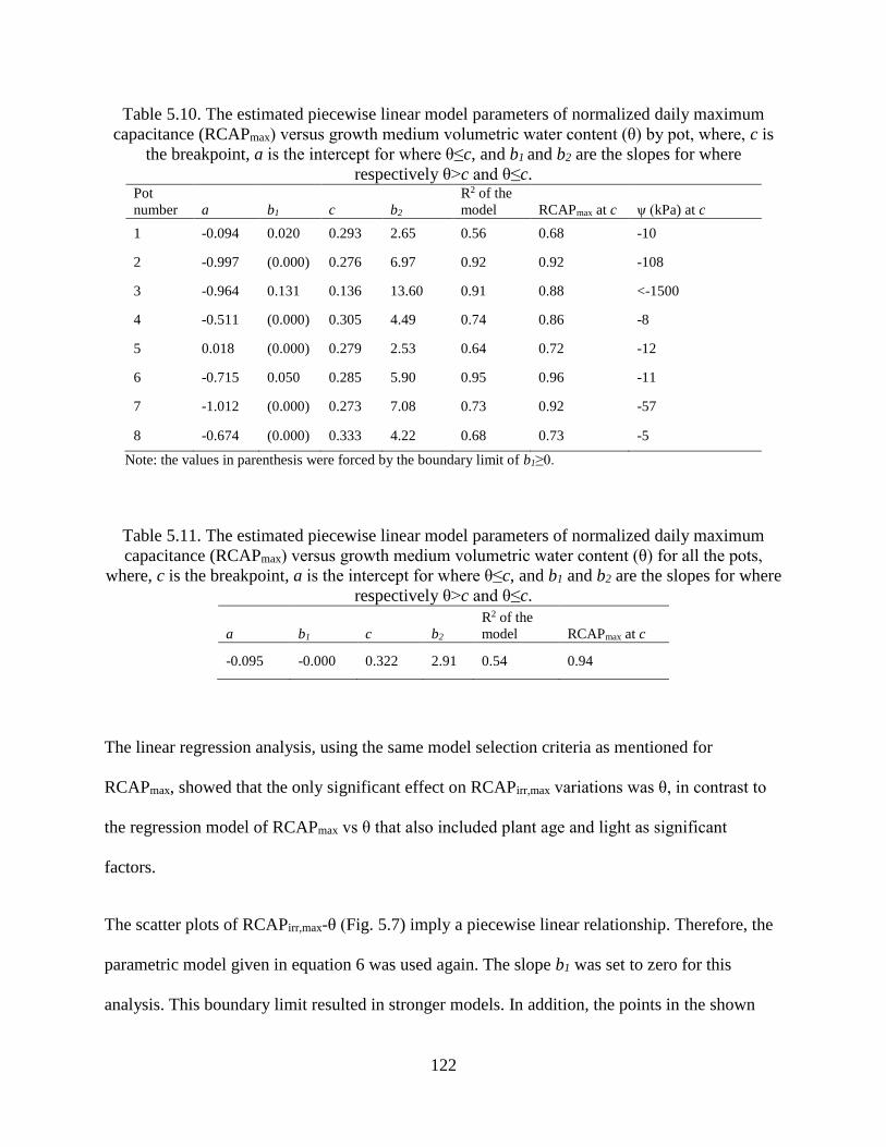
122
Table 5.10. The estimated piecewise linear model parameters of normalized daily maximum
capacitance (RCAPmax) versus growth medium volumetric water content (θ) by pot, where, c is
the breakpoint, a is the intercept for where θ≤c, and b1 and b2 are the slopes for where
respectively θ>c and θ≤c. Pot
number a b1 c b2
R2 of the
model RCAPmax at c ψ (kPa) at c
1 -0.094 0.020 0.293 2.65 0.56 0.68 -10
2 -0.997 (0.000) 0.276 6.97 0.92 0.92 -108
3 -0.964 0.131 0.136 13.60 0.91 0.88 <-1500
4 -0.511 (0.000) 0.305 4.49 0.74 0.86 -8
5 0.018 (0.000) 0.279 2.53 0.64 0.72 -12
6 -0.715 0.050 0.285 5.90 0.95 0.96 -11
7 -1.012 (0.000) 0.273 7.08 0.73 0.92 -57
8 -0.674 (0.000) 0.333 4.22 0.68 0.73 -5
Note: the values in parenthesis were forced by the boundary limit of b1≥0.
Table 5.11. The estimated piecewise linear model parameters of normalized daily maximum
capacitance (RCAPmax) versus growth medium volumetric water content (θ) for all the pots,
where, c is the breakpoint, a is the intercept for where θ≤c, and b1 and b2 are the slopes for where
respectively θ>c and θ≤c.
a b1 c b2
R2 of the
model RCAPmax at c
-0.095 -0.000 0.322 2.91 0.54 0.94
The linear regression analysis, using the same model selection criteria as mentioned for
RCAPmax, showed that the only significant effect on RCAPirr,max variations was θ, in contrast to
the regression model of RCAPmax vs θ that also included plant age and light as significant
factors.
The scatter plots of RCAPirr,max-θ (Fig. 5.7) imply a piecewise linear relationship. Therefore, the
parametric model given in equation 6 was used again. The slope b1 was set to zero for this
analysis. This boundary limit resulted in stronger models. In addition, the points in the shown
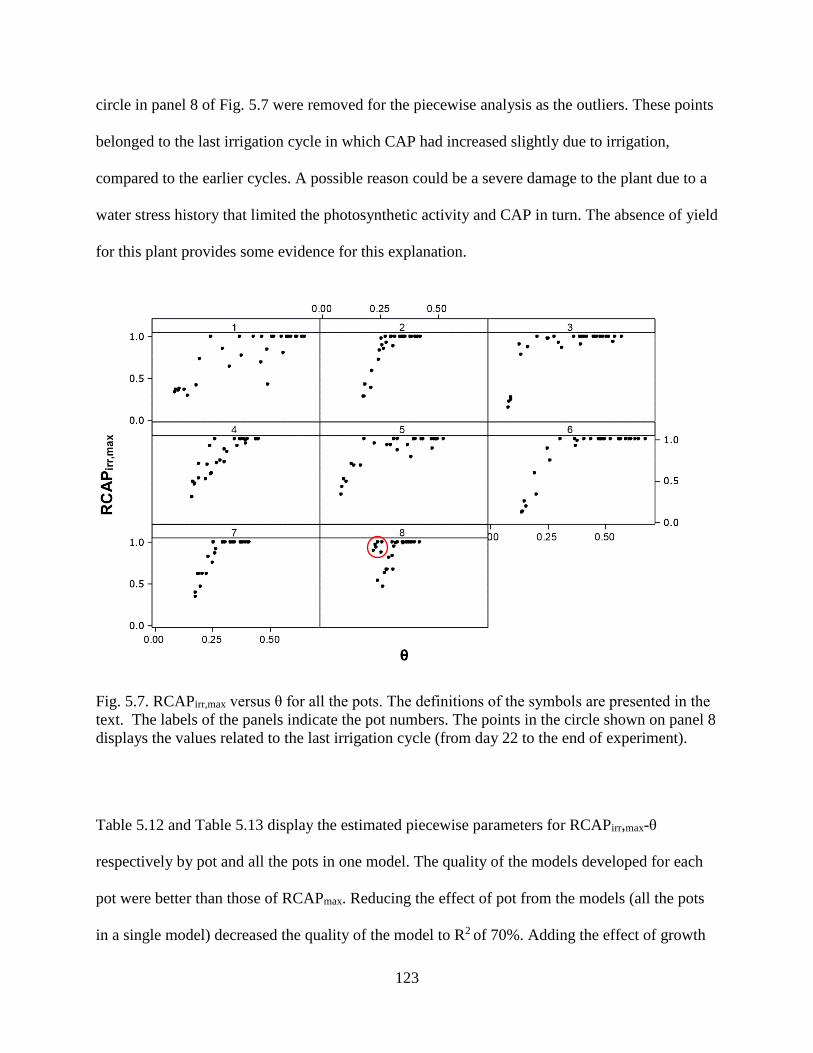
123
circle in panel 8 of Fig. 5.7 were removed for the piecewise analysis as the outliers. These points
belonged to the last irrigation cycle in which CAP had increased slightly due to irrigation,
compared to the earlier cycles. A possible reason could be a severe damage to the plant due to a
water stress history that limited the photosynthetic activity and CAP in turn. The absence of yield
for this plant provides some evidence for this explanation.
Fig. 5.7. RCAPirr,max versus θ for all the pots. The definitions of the symbols are presented in the
text. The labels of the panels indicate the pot numbers. The points in the circle shown on panel 8
displays the values related to the last irrigation cycle (from day 22 to the end of experiment).
Table 5.12 and Table 5.13 display the estimated piecewise parameters for RCAPirr,max-θ
respectively by pot and all the pots in one model. The quality of the models developed for each
pot were better than those of RCAPmax. Reducing the effect of pot from the models (all the pots
in a single model) decreased the quality of the model to R2 of 70%. Adding the effect of growth

124
medium to the model (modeling RCAPirr,max-θ for each medium separately) did not improve the
model as much as the effect of pot. It can be explained by the analysis of variance on the
estimated parameters that showed medium did not significantly affect the estimated parameters
(p-value<0.05).
Table 5.12. The estimated piecewise linear model parameters of RCAPirr,max versus growth
medium volumetric water content (θ) by pot, where, c is the breakpoint, a is the intercept for
where θ≤c, and b1 and b2 are the slopes for where respectively θ>c and θ≤c. The definition of
RCAPirr,max is presented in the text. Pot
number a c b2
R2 of the
model RCAPirr,max at c ψ (kPa) at c
1 -0.108 0.259 3.90 0.71 0.90 -14
2 -1.035 0.276 7.33 0.95 0.99 -107
3 -0.964 0.143 13.60 0.97 0.98 <-1500
4 -0.019 0.354 2.85 0.82 0.99 -5
5 -0.033 0.197 5.08 0.90 0.96 -47
6 -0.684 0.290 5.79 0.97 1.00 -10
7 -0.673 0.277 6.04 0.92 1.00 -54
8 -1.146 0.330 6.49 0.86 1.00 -5
Table 5.13. The estimated piecewise linear model parameters of RCAPirr,max versus growth
medium volumetric water content (θ) for all the pots, where, c is the breakpoint, a is the intercept
for where θ≤c, and b1 and b2 are the slopes for where respectively θ>c and θ≤c. The definition of
RCAPirr,max is presented in the text.
a c b2
R2 of the
model RCAPirr,max at c
0.033 0.325 2.90 0.70 0.98
The estimated breakpoints for RCAPmax and RCAPirr,max were closer to those of RLTmin
compared to RLTmax. Therefore, RCAPmax and RCAPirr,max can possibly be measures for early
identification of plant water stress. However, RCAPirr,max predicted θ better than RCAPmax. In

125
addition, normalizing by CAPirr,m could reduce the effect of plant age from the model, which
resulted in stronger models.
Leaf thickness and capacitance versus water stress levels
Recalling the applied water stress levels across the irrigation cycles, the last day of each
irrigation cycle stands as the designated water stress level for that cycle. For example, for the
irrigation cycle from day 13 to the end of day 16, the plants were not irrigated until observing
signs of visual wilting during night, which reflected a severe water stress level. The effect of
severe water stress on day 16 of the irrigation cycle on θ and the relative critical values of LT
and CAP was investigated.
The analysis of variance showed that water stress level and its interaction with the type of growth
medium were significant for θ (p-value<0.05). Fig. 5.8 and Fig. 5.9 show the interval plots of θ
across the water stress levels for respectively the potting mixture and the mineral soil. For the
potting mixture, the means of θ were significantly different from well-watered to severe water
stress levels while there was no significant difference in θ from severe to desiccation levels (p-
value<0.05). For the mineral soil, the means of θ for each stress level was not statistically
different from θ at the next stress level. These results show that measurement of θ was able to
distinguish well-watered from moderate stress, and moderate stress from severe stress for the
potting mixture but not between severe and desiccation.
In contrast, the means of θ for the mineral soil were not significantly different from the next
stress level. For example, there was only a significant difference between well-watered and
severe water stress level (p-value< 0.05, Fig. 5.9). Therefore, θ for the mineral soil was not

126
suitable for early detection of water stress. As Fig. 5.8 and Fig. 5.9 show, the ranges of the means
of θ were 0.30 for the potting mixture and 0.09 for the mineral soil.
Fig. 5.8. The interval plot of volumetric water content (θ) across the water stress levels for the
pots filled with potting mixture. The brackets display the 95% confidence intervals of the means (ⴲ). The letters indicate the grouping comparison by Tukey method (α=0.05). The means that do
not share a letter are significantly different (p-value<0.05).
In the potting mixture, growth medium matric potential was below -1500 kPa for severe and
extreme water stress levels, with an exception that ψ of one pot was -24 kPa at the severe water
stress level (Fig. 5.10). Growth medium matric potential was in the range of below -1500 kPa to
-50 kPa for the desiccation stress level within the mineral soil (Fig. 5.11). To avoid
extrapolation, the water stress levels at ψ<-1500 kPa were removed from the analysis of
variance. The analysis of variance across the well-watered and moderate water stress levels
showed that medium significantly affected ψ, but there was no interaction of medium with water
stress level (p-value<0.05).
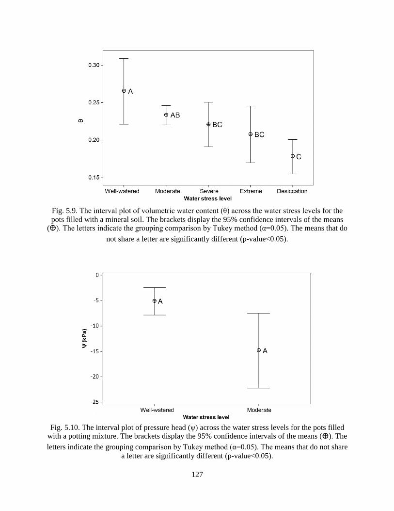
127
Fig. 5.9. The interval plot of volumetric water content (θ) across the water stress levels for the
pots filled with a mineral soil. The brackets display the 95% confidence intervals of the means (ⴲ). The letters indicate the grouping comparison by Tukey method (α=0.05). The means that do
not share a letter are significantly different (p-value<0.05).
Fig. 5.10. The interval plot of pressure head (ψ) across the water stress levels for the pots filled
with a potting mixture. The brackets display the 95% confidence intervals of the means (ⴲ). The
letters indicate the grouping comparison by Tukey method (α=0.05). The means that do not share
a letter are significantly different (p-value<0.05).

128
Fig. 5.11. The interval plot of pressure head (ψ) across the water stress levels for the pots filled
with mineral soil. The brackets display the 95% confidence intervals of the means (ⴲ). The
letters indicate the grouping comparison by Tukey method (α=0.05). The means that do not share
a letter are significantly different (p-value<0.05).
Fig. 5.10 and Fig. 5.11 show that the means of ψ within the growth media were not significantly
different across the water stress levels. Therefore, this suggests that the means of ψ could not be
used to distinguish the water stress levels until it was below the wilting point.
Fig. 5.12 shows the means of night time relative leaf thickness (RLTmax) across the water stress
levels. There was no significant difference between the means of RLTmax from well-watered to
severe water stress while there was a significant difference between severe and desiccation (p-
value<0.05). This suggests RLTmax is sensitive to detect severe water stress but not moderate
water stress.

129
Fig. 5.12. The interval plot of normalized daily maximum leaf thickness (RLTmax) across the water stress levels. The brackets display the 95% confidence intervals of the means (ⴲ). The
letters indicate the grouping comparison by Tukey method (α=0.05). The means that do not share
a letter are significantly different (p-value<0.05).
The analysis of variance showed that growth medium and water stress level significantly affected
RLTmin (p-value<0.05). Therefore, RLTmin was analyzed separately for each medium. Fig. 5.13
displays the means of RLTmin across the water stress levels in the potting mixture. The means
were significantly different between all the water stress levels. For the mineral soil, the means of
RLTmin were significantly different between well-watered and moderate stress levels, but there
was not a significant difference between RLTmin at moderate stress and severe water stress,
although RLTmin at moderate stress was significantly different from that at extreme water stress
(Fig. 5.14).

130
Fig. 5.13. The interval plot of normalized daily minimum leaf thickness (RLTmin) across the
water stress levels for the pots filled with a potting mixture. The brackets display the 95% confidence intervals of the means (ⴲ). The letters indicate the grouping comparison by Tukey
method (α=0.05). The means that do not share a letter are significantly different (p-value<0.05).
Fig. 5.14. The interval plot of normalized daily minimum leaf thickness (RLTmin) across the
water stress levels for the pots filled with a mineral soil. The brackets display the 95% confidence intervals of the means (ⴲ). The letters indicate the grouping comparison by Tukey
method (α=0.05). The means that do not share a letter are significantly different (p-value<0.05).

131
This result suggests that a transition from well-watered to moderate water stress level could be
detected by variations in the noon-time relative thickness (RLTmin) regardless of the growth
medium. However, RLTmin may not be used to detect more severe water stress depending on the
growth medium. Fig. 5.15 shows the means of RLTmin averaged for both growth media. The
means of RLTmin were significantly different between each water stress level except those at
severe and extreme stress level.
Fig. 5.15. The interval plot of normalized daily minimum leaf thickness (RLTmin) across the
water stress levels (regardless of medium). The brackets display the 95% confidence intervals of the means (ⴲ). The letters indicate the grouping comparison by Tukey method (α=0.05). The
means that do not share a letter are significantly different (p-value<0.05).
Fig. 5.16 and Fig. 5.17 present the interval plots of RCAPmax and RCAPirr,max across the water
stress levels. The means of RCAPmax and RCAPirr,max were significantly different between
moderate and severe stress levels, and between extreme and desiccation levels, while there was
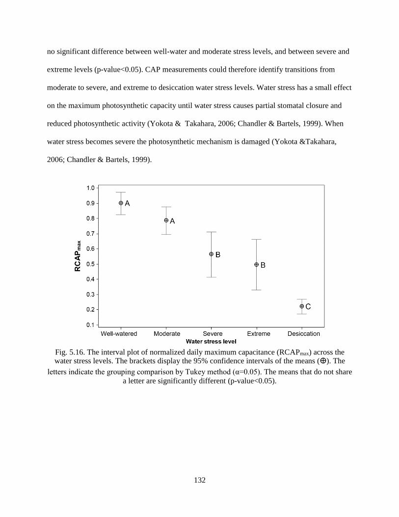
132
no significant difference between well-water and moderate stress levels, and between severe and
extreme levels (p-value<0.05). CAP measurements could therefore identify transitions from
moderate to severe, and extreme to desiccation water stress levels. Water stress has a small effect
on the maximum photosynthetic capacity until water stress causes partial stomatal closure and
reduced photosynthetic activity (Yokota & Takahara, 2006; Chandler & Bartels, 1999). When
water stress becomes severe the photosynthetic mechanism is damaged (Yokota &Takahara,
2006; Chandler & Bartels, 1999).
Fig. 5.16. The interval plot of normalized daily maximum capacitance (RCAPmax) across the water stress levels. The brackets display the 95% confidence intervals of the means (ⴲ). The
letters indicate the grouping comparison by Tukey method (α=0.05). The means that do not share
a letter are significantly different (p-value<0.05).

133
Fig. 5.17. The interval plot of normalized daily maximum capacitance within irrigation cycles
(RCAPirr,max) across the water stress levels. The brackets display the 95% confidence intervals of the means (ⴲ). The letters indicate the grouping comparison by Tukey method (α=0.05). The
means that do not share a letter are significantly different (p-value<0.05).
Although Fig. 5.16 and Fig. 5.17 suggest that RCAPmax and RCAPirr,max behaved similarly across
water stress levels, the pricewise models of RCAPirr,max-θ were stronger than those of RCAPmax-
θ. Therefore, RCAPirr,max may be preferred to determine water stress in plants.
Capacitance as a predictor of yield
Although the objective of this study was to investigate the effects of growth medium water
content and water stress levels on LT and CAP, the relationship between CAP and yield may
help in a better understanding of the mechanism of CAP variations in relation to photosynthetic
activity. If CAP is a gauge of photosynthetic activity, the area below the curve of CAP-time
(CAParea) is an estimate of cumulative photosynthetic activity which should determine yield.
Table 5.14 shows CAParea and fresh yield (fruits) by pot. CAParea and fresh yield were strongly

134
correlated (p-value<0.01; Fig. 5.18), suggesting that CAP can be used as a gauge for
photosynthetic activity to predict the yield. However, this result needs to be validated in other
studies with a larger sample size and more leaf sensors per plant.
Table 5.14. The area below the curve of capacitance-time (CAParea) by pot.
Pot CAParea (pF day) Fresh yield (g)
1 24.2 60
2 18.5 32
3 45.5 347
4 29.4 42
5 35.2 235
6 29.1 275
7 23.0 9
8 17.0 0
Fig. 5.18. Scatter plot of fresh yield versus the area below the curve of capacitance-time
(CAParea) across the pots. The solid line shows the fitted regression line (y = 12.78 x ̶ 229.3, R2
= 0.75, p-value < 0.01).

135
Conclusion
LT and CAP showed daily fluctuations associated with ambient light and growth medium water
content and visual water stress levels. CAP was shown to be a possible indicator of
photosynthetic activity. CAP was roughly at a constant minimum value during the nights and
rapidly increased during the day. The peak of CAP occurred close to noon. However, daily
maximum CAP were positively correlated with θ, possibly showing the effect of water stress on
photosynthetic activity. That CAP could be an indicator of photosynthetic activity was further
confirmed by the observation that the area below the curve of CAP-time (CAParea) was positively
correlated with yield. However, further studies are required to investigate the relationship
between the photosynthetic metabolism and CAP to confirm this.
Factors other than photosynthesis that change leaf solute contents such as osmoregulation may
also affect CAP (Yokota & Takahara, 2006; Farooq et al., 2009; Taiz & Zeiger, 2006). Tomato,
used in this trial, does not exhibit osmoregulation (Rudich & Luchinsky, 1986), but it might
compromise the use of CAP to measure photosynthesis (and water stress) in other crops. Other
factors such as fertilizers and soil salinity may also affect leaf solute contents and CAP readings
(Ashraf & Harris, 2013; Liu, Sung, Chen, & Lai, 2014; Taiz & Zeiger, 2006). Therefore, more
research is warranted to investigate the use of CAP to determine photosynthesis and water stress.
Use of daily maximum and minimums values of LT and maximum values of CAP helped
interpret their effects on water stress. This can also help to reduce computation costs and data
collection intervals, which are essential factors for the efficiency of automatic systems.
The LT and CAP normalization methods used in this study improved comparison of readings
from different leaves and reduced the effects of growth and water stress history.

136
Night-time relative leaf thickness (RLTmax) and noon-time relative thickness (RLTmin) had a
strong piecewise linear relationship with θ. The relationships between the night-time and noon-
time relative LT versus θ (RLTmax-θ and RLTmin-θ) had shallow slopes for θ greater than the
breakpoints and the slopes increased rapidly for θ below the breakpoints. Other researchers also
observed such a piecewise relationship with a distinct breakpoint in the relationship between LT
and leaf water potential (Neumann et al., 1974; Scoffoni et al., 2014). These authors suggested
that this breakpoint corresponds with the turgor loss point (turgor pressure of zero Pa). The
breakpoints of RLTmax-θ occurred at smaller θ values compared to RLTmin-θ, suggesting that the
noon-time relative thickness (RLTmin) was an earlier water stress signal. However, the observed
relationship between RLTmax and θ was stronger than that of RLTmin.
As mentioned earlier, CAP was dependent on the light intensity. Volumetric water content, light,
plant age, and the categorical effect of the pots explained 91% of RCAPmax variations. In
contrast, RCAPirr,max was not dependent on light and plant age. Therefore, the piecewise models
of RCAPirr,max-θ were stronger than those of RCAPmax-θ, suggesting that RCAPirr,max can be a
better gauge for plant water status compared to RCAPmax. However, RCAPmax may be a better
measure of photosynthesis over the plant’s entire life. We therefore suggest RCAPmax as a
general signal for various types of plant stresses which reduce the photosynthetic activity, such
as low light intensity and disease (Selvaraj & Fof, 2012; Taiz & Zeiger, 2006). On the other
hand, RCAPirr,max would be preferred for estimation of water status.
In our study, leaf thickness and capacitance measurement was able to distinguish between water
stress levels better than soil moisture or potential measurements, especially in the topsoil
medium. The night-time relative LT (RLTmax) could clearly identify a transition from severe to
extreme and then to desiccation stress level. Noon-time relative LT (RLTmin), on the other hand,

137
could identify all the stress levels except between severe and extreme levels if data of both
growth mediums were combined. Finally, relative maximum CAP (RCAPmax and RCAPirr,max)
was significantly different between moderate and severe water stress levels, and between
extreme and desiccation stress levels.
Therefore, these results suggest that a combination of the relative values gives a power to clearly
detect each water stress level. For example, RLTmin can be used to recognize a transition from
well-watered to moderate water stress level, while RCAPirr,max and RLTmax may be preferred to
detect a transition for respectively middle and late water stress levels.
The results of this study show great promise to improve measurement of plant water status and
hence irrigation efficiency by using leaf thickness and capacitance instead of soil moisture and
matric potential. The sensors developed in this project allow LT and CAP measurements using
automatic systems for practical applications, such as irrigation scheduling and research purposes.
However, considering the limited number of species, environmental conditions, and management
variables (such as irrigation schedules), more research is needed to test and develop this
technology further.
References
Ackerson, R. C. (1980). Stomatal response of cotton to water stress and abscisic Acid as affected
by water stress history. Plant Physiology, 65(3), 455–9.
Afzal, A., Mousavi, S., & Khademi, M. (2010). Estimation of leaf moisture content by
measuring the capacitance. Journal of Agricultural Science Technology, 12, 339–346.
Ashraf, M., & Harris, P. J. C. (2013). Photosynthesis under stressful environments: An overview.

138
Photosynthetica, 51(2), 163–190.
Aubuchon, R. R., Thompson, D. R., & Hinckley, T. M. (1978). Environmental influences on
photosynthesis withing the crown of a white oak. Oecologia, 35(3), 295–306.
Bachmann, F. (1922). Studien über die dickenänderung von laubblättern. Jahrbücher Für
Wissenschaftliche Botanik, 61, 372–429.
Baxter, L. K. (1996). Capacitive sensors: design and applications. John Wiley & Sons. New
York: John Wiley & Sons.
Brady, N. C. (1990). The nature and properties of soils (10th ed.). New York: Macmillan.
Búrquez, A. (1987). Leaf thickness and water deficit in plants: a tool for field studies. Journal of
Experimental Botany, 38(186), 109–114.
Chandler, J., & Bartels, D. (1999). Plant desiccation. In H. R. Lerner (Ed.), Plant response to
environmental stresses: from phytohormones to genome reorganization (pp. 575–590). New
York: Marcel Dekker.
Clifford, S. C., Arndt, S. K., Corlett, J. E., Joshi, S., Sankhla, N., Popp, M., & Jones, H. G.
(1998). The role of solute accumulation, osmotic adjustment and changes in cell wall
elasticity in drought tolerance in Ziziphus mauritiana (Lamk.). Journal of Experimental
Botany, 49(323), 967–977.
Cohen, Y., Alchanatis, V., Meron, M., Saranga, Y., & Tsipris, J. (2005). Estimation of leaf water
potential by thermal imagery and spatial analysis. Journal of Experimental Botany, 56(417),
1843–1852.

139
Dadshani, S., Kurakin, A., Amanov, S., Hein, B., Rongen, H., Cranstone, S., … Ballvora, A.
(2015). Non-invasive assessment of leaf water status using a dual-mode microwave
resonator. Plant Methods, 11(1), 8.
Damour, G., Simonneau, T., Cochard, H., & Urban, L. (2010). An overview of models of
stomatal conductance at the leaf level. Plant, Cell and Environment, 33(9), 1419–1438.
Dongsheng, L., Manxi, H., Huijuan, W., & Ziqian, W. (2007). Law of fluctuation in plant leaves
thickness during day and night. Journal of Physics: Conference Series, 48, 1447–1452.
Eusufzai, M. K., & Fujii, K. (2012). Effect of organic matter amendment on hydraulic and pore
characteristics of a clay loam soil. Open Journal of Soil Science, 2, 372–381.
Evett, S. R., Heng, L. K., Moutonnet, P., & Nguyen, M. L. (Eds.). (2008). Field estimation of
soil water content: a practical guide to methods, instrumentation and sensor technology.
International Atomic Energy Agency.
Farahani, H., Wagiran, R., & Hamidon, M. (2014). Humidity Sensors Principle, Mechanism, and
Fabrication Technologies: A Comprehensive Review. Sensors, 14(5), 7881–7939.
Farooq, M., Wahid, A., Kobayashi, N., Fujita, D., & Basra, S. M. A. (2009). Plant drought stress:
effects, mechanisms and management. Agronomy for Sustainable Development, 29(1), 185–
212.
Feddes, R., & Raats, P. (2004). Parameterizing the soil-water-plant root system. In R. A. Feddes,
G. H. d. Rooij, & J. C. van Dam (Eds.), Unsaturated-zone modeling: progress, challenges
and applications (pp. 95–141). Dordrecht, Netherlands: Kluwer Academic Publisher.

140
Gall, H., Philippe, F., Domon, J.-M., Gillet, F., Pelloux, J., & Rayon, C. (2015). Cell wall
metabolism in response to abiotic stress. Plants, 4(1), 112–166.
Gente, R., Born, N., Voß, N., Sannemann, W., Léon, J., Koch, M., & Castro-Camus, E. (2013).
Determination of leaf water content from terahertz time-domain spectroscopic data. Journal
of Infrared, Millimeter, and Terahertz Waves, 34(3-4), 316–323.
Giuliani, R., Koteyeva, N., Voznesenskaya, E., Evans, M. A., Cousins, A. B., & Edwards, G. E.
(2013). Coordination of leaf photosynthesis, transpiration, and structural traits in rice and
wild relatives (genus Oryza). Plant Physiology, 162(3), 1632–51.
Grimnes, S., & Martinsen, Ø. G. (2008). Bioimpedance and Bioelectricity Basics (2nd ed.). New
York: Academic Press.
Ishai, P. Ben, Talary, M. S., Caduff, A., Levy, E., & Feldman, Y. (2013). Electrode polarization
in dielectric measurements: a review. Measurement Science and Technology, 24(10), 1–21.
Jones, H. G. (2004). Irrigation scheduling: advantages and pitfalls of plant-based methods.
Journal of Experimental Botany, 55(407), 2427–36.
Jones, H. G. (2014). Plants and microclimate: a quantitative approach to environmental plant
physiology (3rd ed.). Cambridge: Cambridge University Press.
Klute, A. (Ed.). (1986). Methods of soil analysis: part 1—physical and mineralogical methods. In
American Society of Agronomy, Soil Science Society of America (2nd ed.). Madison, WI.
Kramer, P. J., & Boyer, J. S. (1995). Water relations of plants and soils. San Diego: Academic
Press.

141
Liu, C.-W., Sung, Y., Chen, B.-C., & Lai, H.-Y. (2014). Effects of Nitrogen Fertilizers on the
Growth and Nitrate Content of Lettuce (Lactuca sativa L.). International Journal of
Environmental Research and Public Health, 11(4), 4427–4440.
Malone, M. (1993). Rapid inhibition of leaf growth by root cooling in wheat: kinetics and
mechanism. Journal of Experimental Botany, 44(268), 1663–1669.
Marenco, R. a., Antezana-Vera, S. a., & Nascimento, H. C. S. (2009). Relationship between
specific leaf area, leaf thickness, leaf water content and SPAD-502 readings in six
Amazonian tree species. Photosynthetica, 47(2), 184–190.
McBurney, T. (1992). The relationship between leaf thickness and plant water potential. Journal
of Experimental Botany, 43(248), 327–335.
Medrano, H., Escalona, J. M., Bota, J., Gulías, J., & Flexas, J. (2002). Regulation of
photosynthesis of C3 plants in response to progressive drought: Stomatal conductance as a
reference parameter. Annals of Botany, 89(SPEC. ISS.), 895–905.
Meidner, H. (1952). An instrument for the continuous determination of leaf thickness changes in
the field. Journal of Experimental Botany, 3(9), 319–325.
Nemes, A., Rawls, W. J., & Pachepsky, Y. a. (2005). Influence of organic matter on the
estimation of saturated hydraulic conductivity. Soil Science Society of America Journal,
69(4), 1330–1337.
Neumann, H. H., Thurtell, G. W., Stevenson, K. R., & Beadle, C. L. (1974). Leaf water content
and potential in corn, sorghum, soybean, and sunflower. Canadian Journal of Plant

142
Science, 54(1), 185–195.
O’Shaughnessy, S. a., & Evett, S. R. (2010). Canopy temperature based system effectively
schedules and controls center pivot irrigation of cotton. Agricultural Water Management,
97(9), 1310–1316.
Pethig, R. (1979). Dielectric and electronic properties of biological materials. Chichester,
England: Wiley.
Radcliffe, D. E., & Šimunek, J. (2010). Soil physics with Hydrus: modeling and applications.
Boca Raton: CRC Press.
Rozema, J., Arp, W., Diggelen, J., Kok, E., & Letschert, J. (1987). An ecophysiological
comparison of measurements of the diurnal rhythm of the leaf elongation and changes of the
leaf thickness of salt-resistant dicotyledonae and monocotyledonae. Journal of
Experimental Botany, 38(188), 442–453.
Rudich, J., & Luchinsky, U. (1986). Water economy. In J. G. Atherton & J. Rudich (Eds.), The
tomato crop: a scientific basis for improvement (pp. 335–367). London: Chapman and Hall.
Ryan, S. E., & Porth, L. S. (2007). A tutorial on the piecewise regression approach applied to
bedload transport data. General technical report RMRS-GTR-189. General Technical
Report RMRS-GTR-189. Fort Collins, Colorado: U.S. Department of Agriculture, Forest
Service, Rocky Mountain Research Station.
Saseendran, S. A., Ahuja, L. R., Ma, L., Timlin, D., Stöckle, C. O., Boote, K. J., … Yu, Q.
(2008). Current water deficit stress simulations in selected agricultural system models. In L.

143
R. Ahuja, V. R. Reddy, S. A. Saseendran, & Q. Yu (Eds.), Response of crops to limited
water: understanding and modeling water stress effects on plant growth processes,
advances in agricultural systems modeling series 1 (pp. 1–37). American Society of
Agronomy, Crop Science Society of America, Soil Science Society of America.
Schwan, H. P. (1992). Linear and nonlinear electrode polarization and biological materials.
Annals of Biomedical Engineering, 20(3), 269–288.
Scoffoni, C., Vuong, C., Diep, S., Cochard, H., & Sack, L. (2014). Leaf shrinkage with
dehydration: coordination with hydraulic vulnerability and drought tolerance. Plant
Physiology, 164(4), 1772–1788.
Seelig, H. D., Stoner, R. J., & Linden, J. C. (2011). Irrigation control of cowpea plants using the
measurement of leaf thickness under greenhouse conditions. Irrigation Science, 30(4), 247–
257.
Selvaraj, K., & Fof, B. (2012). An overview of plant photosynthesis modulation by pathogen
Attacks. In M. M. Najafpour (Ed.), Advances in Photosynthesis - Fundamental Aspects (pp.
465–486). InTech.
Sharon, Y., & Bravdo, B. (1996). Irrigation control of citrus according to the diurnal cycling of
leaf thickness. In Conference on Water & Irrigation, Tel Aviv, Israel (pp. 273–283).
Sinha, K., & Tabib-Azar, M. (2016). Effect of light and water on Schefflera plant electrical
properties. Journal of Scientific Research and Reports, 9(4), 1–11.
Syvertsen, J., & Levy, Y. (1982). Diurnal changes in citrus leaf thickness, leaf water potential

144
and leaf to air temperature difference. Journal of Experimental Botany, 33(135), 783–789.
Taiz, L., & Zeiger, E. (2006). Plant Physiology (4th ed.). Sunderland, MA: Sinauer Associates.
Vile, D., Garnier, E., Shipley, B., Laurent, G., Navas, M.-L., Roumet, C., … Wright, I. J. (2005).
Specific leaf area and dry matter content estimate thickness in laminar leaves. Annals of
Botany, 96(6), 1129–36.
Vilsack, T., & Reilly, J. T. (2014). 2012 census of agriculture: farm and ranch irrigation survey
(2013). United States Department of Agriculture, National Agricultural Statistics Service
(Vol. 3). United States Department of Agriculture, National Agricultural Statistics Service.
Retrieved August 8, 2016, from
https://www.agcensus.usda.gov/Publications/2012/Online_Resources/Farm_and_Ranch_Irri
gation_Survey/fris13.pdf
Vogel, T., Votrubova, J., Dusek, J., & Dohnal, M. (2016). Mesoscopic aspects of root water
uptake modeling - Hydraulic resistances and root geometry interpretations in plant
transpiration analysis. Advances in Water Resources, 88, 86–96.
Wang, P., & Anderko, a. (2001). Computation of dielectric constants of solvent mixtures and
electrolyte solutions. Fluid Phase Equilibria, 186(1-2), 103–122.
White, J. W., & Montes-R, C. (2005). Variation in parameters related to leaf thickness in
common bean (Phaseolus vulgaris L.). Field Crops Research, 91(1), 7–21.
Yan, W., Zhong, Y., & Shangguan, Z. (2016). A meta-analysis of leaf gas exchange and water
status responses to drought. Scientific Reports, 6(February), 20917.

145
Yokota, A. K., & Takahara, K. A. (2006). Water stress. In K. V. Madhavaro, A. S. Raghavendra,
& K. Janardhanreddy (Eds.), Physiology and molecular biology of stress tolerance in plants
(pp. 15–39). Dordrecht, Netherlands: Springer.
Yoon, G. (2011). Dielectric properties of glucose in bulk aqueous solutions: Influence of
electrode polarization and modeling. Biosensors and Bioelectronics, 26(5), 2347–2353.

146
Chapter 6: Summary and recommendations

147
Summary and recommendations
The goal of this project was to deliver a plant-based technique for monitoring of plant water
status in practical applications. The new advances in electronics enabled to develop small,
affordable, and efficient instrumentations to monitor leaf thickness and electrical capacitance
without damaging the leaf. The next question is how these measurements can be translated to
plant water status. Therefore, the focus of this project was to assess and determine the
relationship of leaf thickness (LT) and capacitance (CAP) measurements with plant water status.
For this project, a small leaf sensor was developed that measured LT and CAP. In addition, a
data acquisition system was designed that had the capability to wirelessly collect the
measurements of several leaf sensors in a greenhouse or field. The results showed that the leaf
sensor could precisely measure CAP and LT.
The first experiment showed that the pattern of leaf relative water content (RWC) versus relative
leaf thickness (RLT) was consistent across four crops and three leaf locations on the plants. The
relationships could be determined by piecewise linear regression with a distinct breakpoint such
that the slope of RWC-RLT variations was shallow for water contents close to full turgor and
steep below the breakpoint. The results suggested that the breakpoint could be an indicator of a
critical water status, probably turgor loss point (turgor pressure of 0 Pa), that causes dramatic
changes in the leaf physiological behavior.
The breakpoints occurred at various values of RLT across the species. RLT at the breakpoints
may be related to the drought and salt tolerance of the crops. If so, the breakpoints may be
indicators of crop drought tolerance. This hypothesis needs to be examined in further studies. In
addition, the breakpoints varied across different leaf locations on a plant. These results imply

148
different RLT thresholds (for example the breakpoints) as critical water stress levels based on the
species and leaf locations.
In the second experiment, the responses of LT and CAP to the variations of growth medium
water content were studied. RLT was negatively associated with light, which reflected the
negative impact of transpiration rate on the leaf water balance. The extent of these daily
variations was small and consistent from field capacity to wilting point. The daily fluctuations
increased below wilting point. In this range, the daily minimum and maximum RLT were smaller
than the previous day such that RLT had an overall descending trend.
Capacitance was positively related to light. It was at a constant minimum value during the dark
periods and rapidly increased by light. The daily maximum CAP (day-time CAP) decreased and
finally ceased under water stress. The results suggested that CAP was related to the leaf
photosynthetic activity and the effect of water stress on CAP was through reducing the rate of
photosynthetic activity.
As a general conclusion for the second experiment, clear and consistent responses of RLT and
CAP to water stress across all the leaves promise that the analysis of RLT and CAP dynamics
can be used to estimate plant water status. The results suggested that an increase in the daily RLT
fluctuations, a smaller night-time RLT, a smaller day-time RLT, or a smaller day-time CAP can
be indicators of water stress.
The third experiment supported the findings of the second experiment. Daily LT fluctuations
were small and consistent for well-watered conditions and increased by water stress. CAP was
consistently at a minimum value during nights and increased by light. Water stress had a
negative impact on the daily maximum CAP (noon-time CAP).

149
The daily minimum and maximum LT (noon- and night-time LT) and the noon-time CAP were
extracted from the data as the daily critical values, and normalized by some proposed procedures
to calculate their relative values. The relative values of critical LT and CAP had a piecewise
linear relationship with the growth medium volumetric water content (θ). The relative values had
little variations for the range of θ from the field capacity to a breakpoint where the rate of
variations increased rapidly for a given reduction in θ. The results suggest that the breakpoints or
a large decrease in the relative values of daily critical LT or CAP could be indicators of critical
water conditions. Since the breakpoint for the night-time relative LT occurred at a smaller θ than
those of noon-time relative CAP and noon-time relative LT, the later relative values would be
preferred for early detection of water stress.
Another analysis compared the performance of soil moisture measurements (θ and matric
potential) and the relative values of LT and CAP for identifying various water stress levels. The
results suggested that transition from a water stress level to a more severe level may not be
detected by soil matric potential measurements until it drops below the wilting point, which can
be considered as a late water stress signal. Soil volumetric water content measurements may suit
for early detection of water stress depending on the growth medium. Soil water content
measurements could identify the early water stress levels for the potting mixture, while the
measurements could not distinguish the water stress level for the mineral soil. Since the majority
of the growth media in the real-world applications are mineral soils, the results suggested that
soil moisture measurements do not suit for early detection of water stress.
The results suggested that the night-time relative LT can be used to clearly detect the severe
water stress levels. Noon-time relative LT clearly identified all the water stress levels for the
potting mixture. For the mineral soil, it could distinguish the early water stress levels but not the

150
middle-range and late stress levels. The means of the noon-time relative CAP were significantly
different for the mid-range water stress levels. Therefore, these results suggest that a
combination of the relative values of the daily critical LT and CAP measurements can provide an
opportunity to clearly detect each water stress level.
In addition, the results suggested that CAP measurement may be used as a measure of
photosynthetic activity that may be useful for detection of plant stresses impacting
photosynthesis (not only water stress) and impacting the yield. The effect of photosynthesis on
CAP was explained by the effect of photosynthesis on the leaf solutes. It is recognized that other
factors can change the solute contents and concentrations of the leaf may have impact on CAP.
For example, some crops have osmoregulatory mechanisms to tolerate drought stress by
accumulating solutes in the leaf (Taiz & Zeiger, 2006). Therefore, CAP may increase as a result
of increased solute concentrations induced by the water stress response of these crops. Thus,
more detailed studies are required to assess the mechanism of CAP variations in response to the
plant physiological behavior and investigate the CAP dynamics across various crops. In addition,
a capacitive sensor with a higher measurement frequency may result in reducing the effect of
solute variations (Grimnes & Martinsen, 2008; Ishai et al., 2013; Pethig, 1979; Schwan, 1992;
Yoon, 2011). However, this approach can result in smaller CAP values and larger noise that
decreases the precision and accuracy of measurements (Afzal et al., 2010; Pethig, 1979).
Finally, the results suggest a promising opportunity to apply LT and CAP measurements for
precision estimation of plant water status. The last experiment presented methods of extracting
and normalizing the daily critical values of LT and CAP dynamics that can be efficiently
implemented into automatic systems for practical applications, such as irrigation scheduling and
research purposes. However, it is important to recognize that the results of this study were

151
observed in a under controlled conditions, with few species, growth chamber or greenhouse
conditions, and short length of the experiments. Further studies are needed to assess the
variability of the relationships of LT and CAP with plant water status for different species, more
variable environmental conditions (e.g. field condition), and different growth stages.
References
Afzal, A., Mousavi, S., & Khademi, M. (2010). Estimation of leaf moisture content by
measuring the capacitance. Journal of Agricultural Science Technology, 12, 339–346.
Grimnes, S., & Martinsen, Ø. G. (2008). Data and models. In Bioimpedance and Bioelectricity
Basics (2nd ed., pp. 283–332). New York: Elsevier.
Ishai, P. Ben, Talary, M. S., Caduff, A., Levy, E., & Feldman, Y. (2013). Electrode polarization
in dielectric measurements: a review. Measurement Science and Technology, 24(10), 1–21.
Pethig, R. (1979). Dielectric and electronic properties of biological materials. Chichester,
England: Wiley.
Schwan, H. P. (1992). Linear and nonlinear electrode polarization and biological materials.
Annals of Biomedical Engineering, 20(3), 269–288.
Taiz, L., & Zeiger, E. (2006). Plant Physiology (4th ed.). Sunderland, MA: Sinauer Associates.
Yoon, G. (2011). Dielectric properties of glucose in bulk aqueous solutions: Influence of
electrode polarization and modeling. Biosensors and Bioelectronics, 26(5), 2347–2353.

152
Appendix A: Retention curves for the pots in Chapter 5
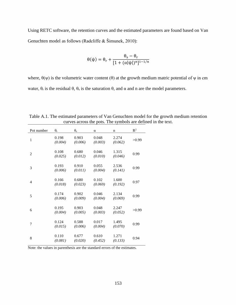
153
Using RETC software, the retention curves and the estimated parameters are found based on Van
Genuchten model as follows (Radcliffe & Šimunek, 2010):
θ(ψ) = θr +θs − θr
[1 + (α|ψ|)n]1−1 n⁄
where, θ(ψ) is the volumetric water content (θ) at the growth medium matric potential of ψ in cm
water, θr is the residual θ, θs is the saturation θ, and α and n are the model parameters.
Table A.1. The estimated parameters of Van Genuchten model for the growth medium retention
curves across the pots. The symbols are defined in the text.
Pot number θr θs α n R2
1 0.198 0.903 0.048 2.274
>0.99 (0.004) (0.006) (0.003) (0.062)
2 0.108 0.680 0.046 1.315
0.99 (0.025) (0.012) (0.010) (0.046)
3 0.193 0.910 0.055 2.536
0.99 (0.006) (0.011) (0.004) (0.141)
4 0.166 0.680 0.102 1.600
0.97 (0.018) (0.023) (0.069) (0.192)
5 0.174 0.902 0.046 2.134
0.99 (0.006) (0.009) (0.004) (0.069)
6 0.195 0.903 0.048 2.247
>0.99 (0.004) (0.005) (0.003) (0.052)
7 0.124 0.588 0.017 1.495
0.99 (0.015) (0.006) (0.004) (0.070)
8 0.110 0.677 0.610 1.271
0.94 (0.081) (0.020) (0.452) (0.133)
Note: the values in parenthesis are the standard errors of the estimates.

154
Fig. A.1. Retention curve for the pot 1 filled with a potting mixture. θ and ψ are respectively
volumetric water content and pressure head.
Fig. A.2. Retention curve for the pot 2 filled with a mineral soil. θ and ψ are respectively
volumetric water content and pressure head.

155
Fig. A.3. Retention curve for the pot 3 filled with a potting mixture. θ and ψ are respectively
volumetric water content and pressure head.
Fig. A.4. Retention curve for the pot 4 filled with a mineral soil. θ and ψ are respectively
volumetric water content and pressure head.

156
Fig. A.5. Retention curve for the pot 5 filled with a potting mixture. θ and ψ are respectively
volumetric water content and pressure head.
Fig. A.6. Retention curve for the pot 6 filled with a potting mixture. θ and ψ are respectively
volumetric water content and pressure head.

157
Fig. A.7. Retention curve for the pot 7 filled with a mineral soil. θ and ψ are respectively
volumetric water content and pressure head.
Fig. A.8. Retention curve for the pot 8 filled with a mineral soil. θ and ψ are respectively
volumetric water content and pressure head.

158
Reference
Radcliffe, D. E., & Šimunek, J. (2010). Soil physics with Hydrus: modeling and applications.
Boca Raton: CRC Press.

159
Appendix B: Graphs of sensor measurements in Chapter 5
Leaf thickness, leaf electrical capacitance, and growth medium volumetric water content for the
pots in Chapter 5
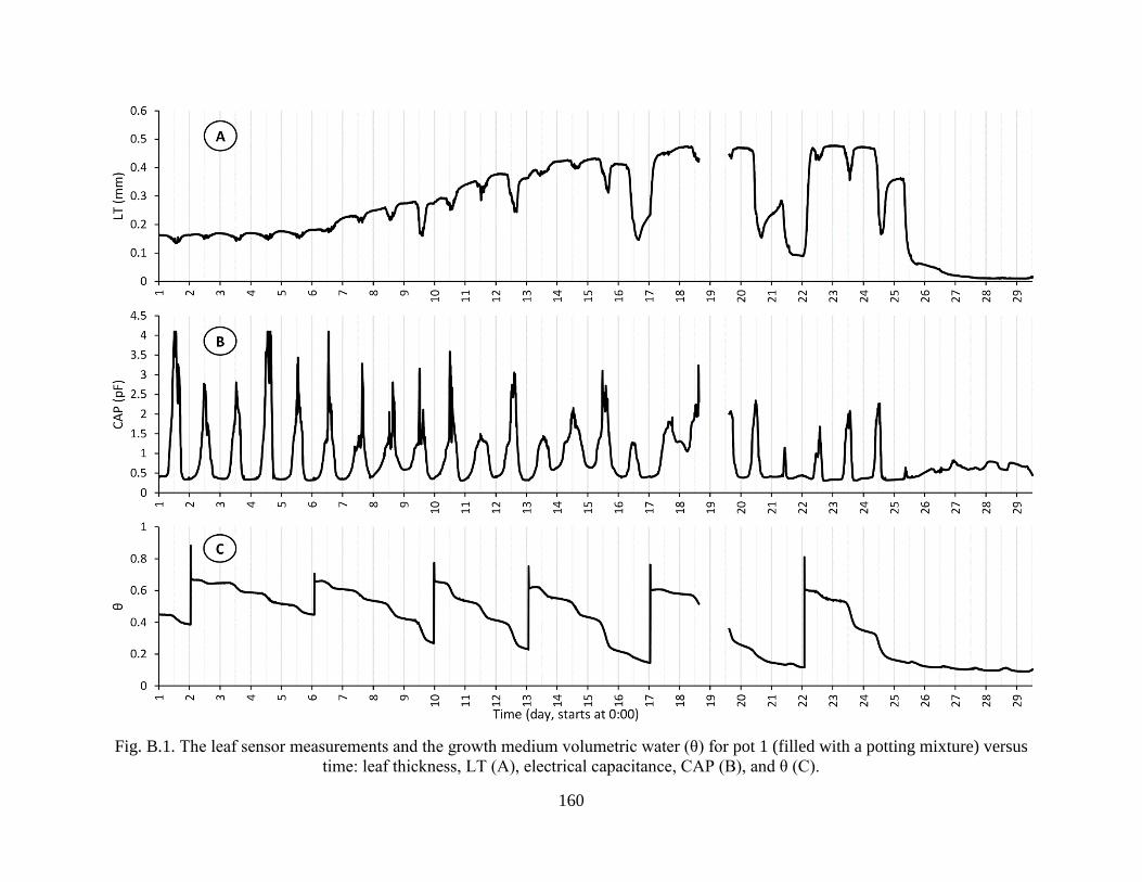
160
Fig. B.1. The leaf sensor measurements and the growth medium volumetric water (θ) for pot 1 (filled with a potting mixture) versus
time: leaf thickness, LT (A), electrical capacitance, CAP (B), and θ (C).

161
Fig. B.2. The leaf sensor measurements and the growth medium volumetric water (θ) for pot 2 (filled with a mineral soil) versus time:
leaf thickness, LT (A), electrical capacitance, CAP (B), and θ (C).

162
Fig. B.3. The leaf sensor measurements and the growth medium volumetric water (θ) for pot 3 (filled with a potting mixture) versus
time: leaf thickness, LT (A), electrical capacitance, CAP (B), and θ (C).
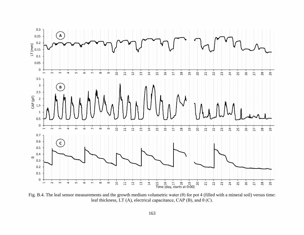
163
Fig. B.4. The leaf sensor measurements and the growth medium volumetric water (θ) for pot 4 (filled with a mineral soil) versus time:
leaf thickness, LT (A), electrical capacitance, CAP (B), and θ (C).
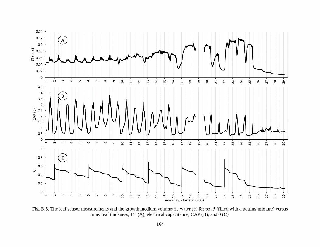
164
Fig. B.5. The leaf sensor measurements and the growth medium volumetric water (θ) for pot 5 (filled with a potting mixture) versus
time: leaf thickness, LT (A), electrical capacitance, CAP (B), and θ (C).

165
Fig. B.6. The leaf sensor measurements and the growth medium volumetric water (θ) for pot 6 (filled with a potting mixture) versus
time: leaf thickness, LT (A), electrical capacitance, CAP (B), and θ (C).

166
Fig. B.7. The leaf sensor measurements and the growth medium volumetric water (θ) for pot 7 (filled with a mineral soil) versus time:
leaf thickness, LT (A), electrical capacitance, CAP (B), and θ (C).

167
Fig. B.8. The leaf sensor measurements and the growth medium volumetric water (θ) for pot 8 (filled with a mineral soil) versus time:
leaf thickness, LT (A), electrical capacitance, CAP (B), and θ (C).

168
Appendix C: Correlation tables of Chapter 5
The tables of correlation matrices for growth medium physical properties, plant dry mass, fresh
yield (fruit), and the estimated piecewise parameters of relative leaf thickness and capacitance
versus growth medium volumetric content, related to the Chapter 5

169
Table C.1. Pearson correlation coefficients of the growth medium physical properties versus
plant dry mass, leaf dry mass, and fresh yield (the definition of the abbreviations and symbols are
provided in the text). The values in the parenthesis show the p-values of the correlation analysis.
BD Ks θs θwp θFC
Plant dry mass -0.66 0.73 0.75 0.75 0.71
(0.077) (0.039) (0.031) (0.030) (0.050)
Fresh yield -0.80 0.76 0.80 0.57 0.66
(0.016) (0.027) (0.016) (0.137) (0.076)
WUE (g lit-1) -0.75 0.71 0.76 0.51 0.60
(0.031) (0.047) (0.027) (0.197) (0.117)
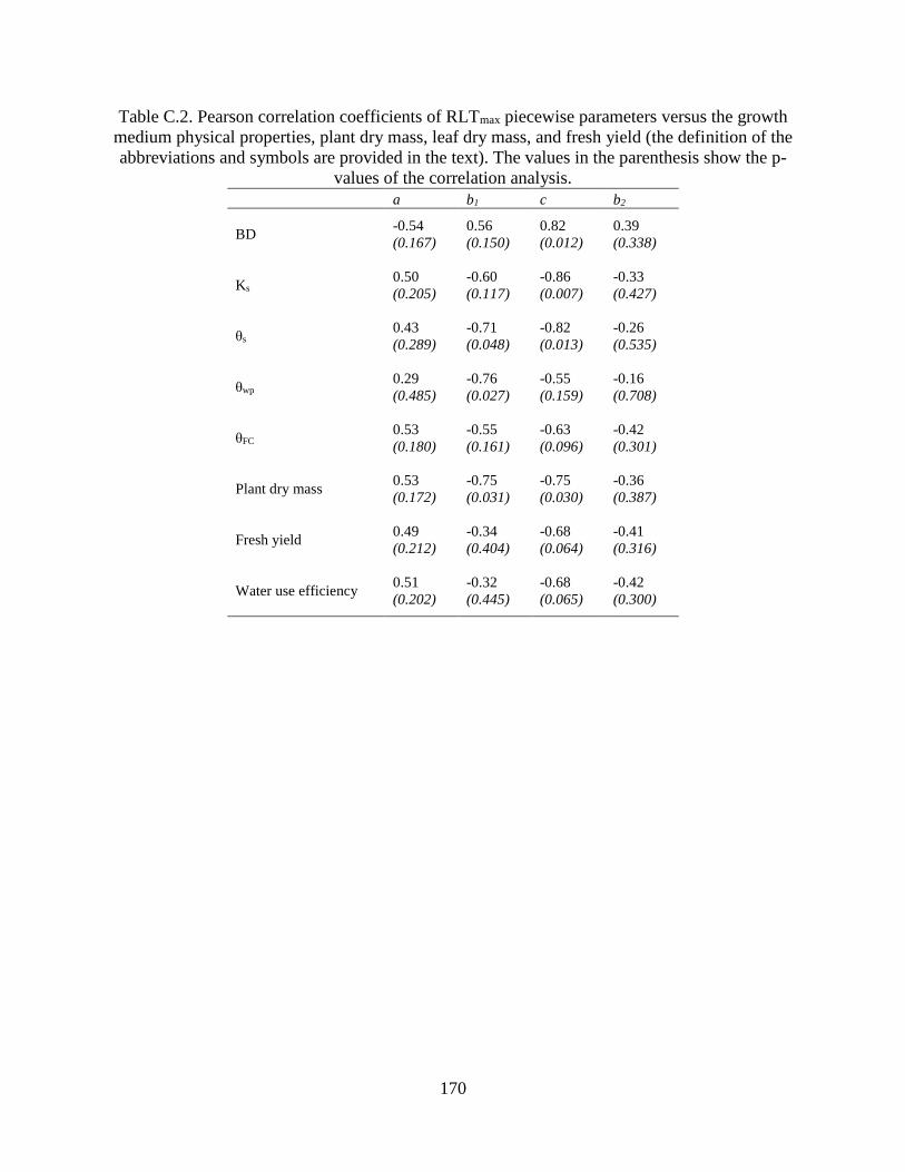
170
Table C.2. Pearson correlation coefficients of RLTmax piecewise parameters versus the growth
medium physical properties, plant dry mass, leaf dry mass, and fresh yield (the definition of the
abbreviations and symbols are provided in the text). The values in the parenthesis show the p-
values of the correlation analysis.
a b1 c b2
BD -0.54 0.56 0.82 0.39
(0.167) (0.150) (0.012) (0.338)
Ks 0.50 -0.60 -0.86 -0.33
(0.205) (0.117) (0.007) (0.427)
θs 0.43 -0.71 -0.82 -0.26
(0.289) (0.048) (0.013) (0.535)
θwp 0.29 -0.76 -0.55 -0.16
(0.485) (0.027) (0.159) (0.708)
θFC 0.53 -0.55 -0.63 -0.42
(0.180) (0.161) (0.096) (0.301)
Plant dry mass 0.53 -0.75 -0.75 -0.36
(0.172) (0.031) (0.030) (0.387)
Fresh yield 0.49 -0.34 -0.68 -0.41
(0.212) (0.404) (0.064) (0.316)
Water use efficiency 0.51 -0.32 -0.68 -0.42
(0.202) (0.445) (0.065) (0.300)
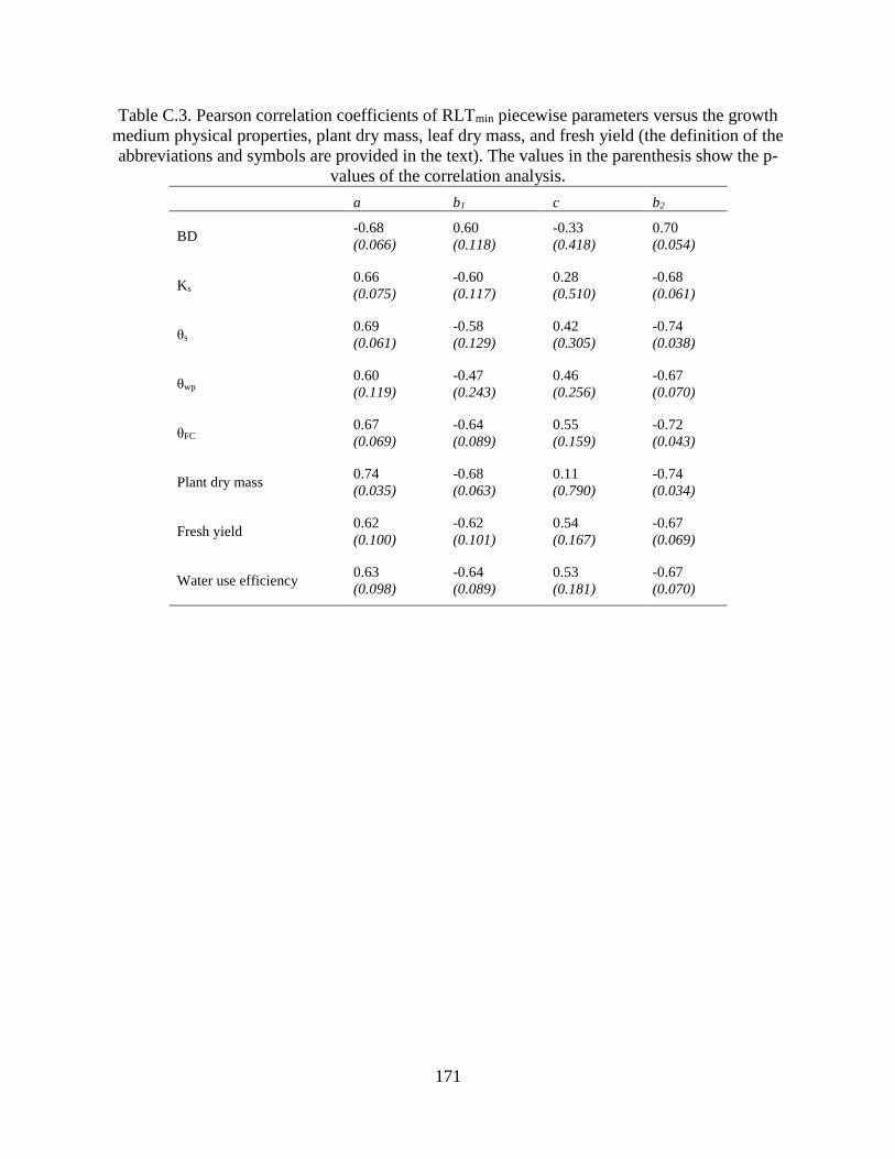
171
Table C.3. Pearson correlation coefficients of RLTmin piecewise parameters versus the growth
medium physical properties, plant dry mass, leaf dry mass, and fresh yield (the definition of the
abbreviations and symbols are provided in the text). The values in the parenthesis show the p-
values of the correlation analysis.
a b1 c b2
BD -0.68 0.60 -0.33 0.70
(0.066) (0.118) (0.418) (0.054)
Ks 0.66 -0.60 0.28 -0.68
(0.075) (0.117) (0.510) (0.061)
θs 0.69 -0.58 0.42 -0.74
(0.061) (0.129) (0.305) (0.038)
θwp 0.60 -0.47 0.46 -0.67
(0.119) (0.243) (0.256) (0.070)
θFC 0.67 -0.64 0.55 -0.72
(0.069) (0.089) (0.159) (0.043)
Plant dry mass 0.74 -0.68 0.11 -0.74
(0.035) (0.063) (0.790) (0.034)
Fresh yield 0.62 -0.62 0.54 -0.67
(0.100) (0.101) (0.167) (0.069)
Water use efficiency 0.63 -0.64 0.53 -0.67
(0.098) (0.089) (0.181) (0.070)

172
Table C.4. Pearson correlation coefficients of RCAPmax piecewise parameters versus the growth
medium physical properties, plant dry mass, leaf dry mass, and fresh yield (the definition of the
abbreviations and symbols are provided in the text). The values in the parenthesis show the p-
values of the correlation analysis.
a b1 c b2
BD -0.50 -0.58 0.43 -0.06
(0.206) (0.133) (0.289) (0.891)
Ks 0.56 0.50 -0.38 -0.01
(0.148) (0.203) (0.349) (0.974)
θs 0.49 0.58 -0.42 0.06
(0.215) (0.131) (0.302) (0.884)
θwp 0.57 0.22 0.00 -0.28
(0.141) (0.605) (0.993) (0.504)
θFC 0.38 0.52 -0.29 0.02
(0.358) (0.192) (0.482) (0.967)
Plant dry mass 0.61 0.19 -0.18 -0.20
(0.106) (0.661) (0.675) (0.629)
Fresh yield 0.06 0.79 -0.70 0.48
(0.886) (0.020) (0.049) (0.230)
Water use efficiency 0.00 0.82 -0.76 0.55
(0.995) (0.014) (0.028) (0.160)

173
Table C.5. Pearson correlation coefficients of RCAPirr,max piecewise parameters versus the
growth medium physical properties, plant dry mass, leaf dry mass, and fresh yield (the definition
of the abbreviations and symbols are provided in the text). The values in the parenthesis show
the p-values of the correlation analysis.
a c b2
BD -0.37 0.65 -0.19
(0.368) (0.084) (0.649)
Ks 0.38 -0.66 0.16
(0.349) (0.074) (0.711)
θs 0.26 -0.64 0.25
(0.527) (0.089) (0.554)
θwp 0.31 -0.28 -0.11
(0.454) (0.503) (0.798)
θFC 0.31 -0.41 0.06
(0.453) (0.308) (0.884)
Plant dry mass 0.54 -0.4 -0.12
(0.166) (0.327) (0.784)
Fresh yield 0.01 -0.74 0.56
(0.975) (0.038) (0.146)
Water use efficiency -0.02 -0.76 0.62
(0.967) (0.029) (0.102)

VITAE
SAYED AMIN AFZAL
BIRTH
LOCATION/
DATE:
Esfahan, Iran. January 27, 1983.
FAMILY: Azadeh Sanayi Ostovar (wife), Sayed Mostafa Afzal and Batoul
Pourabadeh (parents).
EDUCATION: The Pennsylvania State University, PA
Agronomy
Doctor of Philosophy
Isfahan University of Technology, Esfahan, Iran
Agricultural Machinery Engineering
Bachelor of Science
PUBLICATIONS: Afzal, A., Duiker, S., Watson, J., & Luthe, D. (accepted 11/21/2016,
pending revision). A leaf sensor to estimate plant water status and
photosynthetic activity (submitted to Transactions of the ASABE).
Afzal, A., Duiker, S., & Watson, J. (accepted 9/21/2016, pending
revision). Leaf thickness to predict plant water status (submitted to
Biosystems Engineering).
Afzal, A., Mousavi, F., & Khademi, M. (2010). Estimation of leaf
moisture by measuring capacitance. Journal of Agricultural Science
and Technology, 12, 339-346.
H. Aghayeghazvini, A. Afzal, M. Heidarisoltanabadi, S. Malek, & L.
Mollabashi. (2009). Determining percentage of broken rice by using
image analysis. In D. Li, & Z. Chunjiang (Eds.). Computer and
Computing Technologies in Agriculture (Vol. 2), International
Federation for Information Processing (pp. 1019–1027). Springer.
Afzal, A., & Mousavi, F. (2008). Estimation of leaf moisture in maize
by measuring leaf dielectric constant. International Journal of
Agriculture and Biology, 10, 66-68.
HONORS: 2nd place of the 30th Graduate Exhibition. Pennsylvania State
University.
1st place of Dow Sustainability Innovation Student Challenge.
Pennsylvania State University.
1st place of Ag. Springboard Competition. Pennsylvania State
University.