layer-wise cnn surgery for visual sentiment prediction€¦ · layer-wise cnn surgery for visual...
TRANSCRIPT
LAYER-WISE CNN SURGERY FOR VISUAL SENTIMENT PREDICTION
A Degree Thesis
Submitted to the Faculty of the
Escola Tècnica d'Enginyeria de Telecomunicació de
Barcelona
Universitat Politècnica de Catalunya
by
Víctor Campos Camúñez
In partial fulfilment
of the requirements for the degree in
SCIENCE and TELECOMMUNICATION TECHNOLOGIES
ENGINEERING
Advisors:
Xavier Giró (Universitat Politècnica de Catalunya)
Brendan Jou (Columbia University)
Amaia Salvador (Universitat Politècnica de Catalunya)
Barcelona, July 2015

1
Abstract
Visual media are powerful means of expressing emotions and sentiments. The constant generation of new content in social networks highlights the need of automated visual sentiment analysis tools. While Convolutional Neural Networks (CNNs) have established a new state-of-the-art in several vision problems, their application to the task of sentiment analysis is mostly unexplored and there are few studies regarding how to design CNNs for this purpose. In this work, we study the suitability of fine-tuning a CNN for visual sentiment prediction as well as explore performance boosting techniques within this deep learning setting. Finally, we provide a deep-dive analysis into a benchmark, state-of-the-art network architecture to gain insight about how to design patterns for CNNs on the task of visual sentiment prediction.

2
Resum
Els continguts audiovisuals són un mitjà molt poderós per tal d’expressar emocions i
sentiments. La contínua generació de nou contingut en les xarxes socials destaca la
necessitat de disposar d’eines d’anàlisi automàtic de sentiments visuals. Mentre que les
Xarxes Neuronal Convolucionals (de l’anglès, CNNs) han establert l’estat de l’art en
nombrosos problemes de visió, la seva aplicació a l’anterior tasca roman pràcticament
inexplorada i disposem de molt poc coneixement sobre com dissenyar CNNs per aquest
propòsit. En aquest treball estudiem la viabilitat de fer fine-tuning sobre una CNN per
predicció de sentiments visuals i explorem l’ús de tècniques de millora de rendiment de
deep learning (aprenentatge profund). Finalment, desenvolupem un profund anàlisi
d’aquesta arquitectura per tal d’entendre millor el disseny de CNNs per la tasca de
predicció de sentiments visuals.

3
Resumen
Los contenidos audiovisuales son un medio muy poderoso para expresar emociones y
sentimientos. La constante generación de nuevos contenidos en las redes sociales
destaca la necesidad de disponer de herramientas capaces de realizar un análisis
automático de sentimientos visuales. Mientras las Redes Neuronales Convolucionales
(del inglés, CNNs) han establecido el estado del arte en numerosos problemas de visión,
su aplicación a la anterior tarea permanece prácticamente inexplorada y se dispone de
muy poco conocimiento sobre cómo diseñar CNNs para tal propósito. En este trabajo
estudiamos la viabilidad de hacer fine-tuning sobre una CNN para la tarea de predicción
de sentimientos visuales y exploramos técnicas de mejora de rendimiento de deep
learning (aprendizaje profundo). Finalmente, desarrollamos un profundo análisis de la
anterior arquitectura con el objetivo de entender mejor el diseño de CNNs para la tarea
de predicción de sentimientos visuales.

4
Para mi madre, Mari, por ser mi bastón en el
largo camino.
Para mi padre, Paco, por ser un ejemplo día tras
día de la cultura del esfuerzo.
Y para mi abuelo, Pruden, por su apoyo
incondicional durante todos estos años.

5
Acknowledgements
In the first place, I would like to thank my three advisors, Amaia Salvador, Brendan Jou
and Xavi Giró, for their support and guidance during this thesis, as well as for giving me
the chance of taking part in such an interesting project.
I am very grateful to Albert Gil and Josep Pujal for their help with technical problems
during these last months.
I also want to thank my colleagues in the X-Theses and DeepGPI meetings for their ideas
and help in the development of this project.
We gratefully acknowledge the support of NVIDIA Corporation with the donation of
the GeoForce GTX Titan Z used in this work.
Finalment, voldria fer una menció especial als companys de fatigues durant els últims
anys: Chema, Ferran, Fullana, Jiménez, Romero. Sense vosaltres aquest projecte no
hauria estat possible.

6
Revision history and approval record
Revision Date Purpose
0 22/06/2015 Document creation
1 08/07/2015 Document revision
2 09/07/2015 Document approval
DOCUMENT DISTRIBUTION LIST
Name e-mail
Víctor Campos [email protected]
Xavier Giró [email protected]
Amaia Salvador [email protected]
Brendan Jou [email protected]
Written by: Reviewed and approved by:
Date 22/06/2015 Date 09/07/2015
Name Víctor Campos Name Xavier Giró
Position Project Author Position Project Supervisor
7
Table of contents
Abstract ............................................................................................................................ 1
Resum .............................................................................................................................. 2
Resumen .......................................................................................................................... 3
Acknowledgements .......................................................................................................... 5
Revision history and approval record ................................................................................ 6
Table of contents .............................................................................................................. 7
List of Figures ................................................................................................................... 9
List of Tables .................................................................................................................. 10
1. Introduction .............................................................................................................. 11
1.1. Motivation and contributions ............................................................................. 11
1.2. Work plan ......................................................................................................... 12
1.3. Incidences and modifications to the original work plan ..................................... 13
2. State of the art ......................................................................................................... 14
3. Methodology ............................................................................................................ 15
3.1. Convolutional Neural Networks ......................................................................... 15
3.2. K-fold cross-validation ...................................................................................... 16
3.3. Experimental setup ........................................................................................... 16
3.3.1. Fine-tuning CaffeNet ................................................................................. 17
3.3.2. Layer by layer analysis .............................................................................. 18
3.3.3. Layer ablation ............................................................................................ 18
3.3.3.1. Raw ablation ........................................................................................... 19
3.3.3.2. 2-neuron on top ....................................................................................... 19
3.3.4. Layer addition ............................................................................................ 19
3.3.5. Results visualization .................................................................................. 20
3.3.5.1. Score histograms .................................................................................... 20
3.3.5.2. t-Distributed Stochastic Neighbor Embedding (t-SNE) ............................ 20
3.3.5.3. Top-K scores ........................................................................................... 21
3.3.5.4. Receptive fields ....................................................................................... 21
4. Results .................................................................................................................... 22
4.1. Evaluation metric: Accuracy ............................................................................. 22
4.2. Fine-tuning CaffeNet ........................................................................................ 22
4.3. Layer by layer analysis ..................................................................................... 23
4.4. Layer ablation ................................................................................................... 24
8
4.5. Layer addition ................................................................................................... 25
4.6. Results visualization ......................................................................................... 25
4.6.1. Score histograms ...................................................................................... 25
4.6.2. t-Distributed Stochastic Neighbor Embedding (t-SNE) ............................... 26
4.6.3. Top-K scores ............................................................................................. 28
4.6.4. Receptive fields ......................................................................................... 29
5. Budget ..................................................................................................................... 31
6. Conclusions and future work.................................................................................... 32
Bibliography: ................................................................................................................... 33
Appendix 1: Work packages ........................................................................................... 35
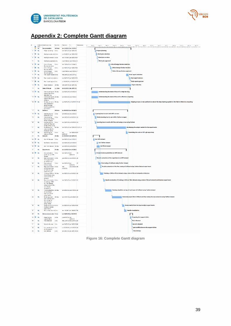
Appendix 2: Complete Gantt diagram ............................................................................. 39
Glossary ......................................................................................................................... 40
9
List of Figures
Figure 1: Gantt diagram .................................................................................................. 13
Figure 2: Single neuron diagram ..................................................................................... 15
Figure 3: Multi-layer Neural Network ............................................................................... 15
Figure 4: Pipeline of the proposed Visual Sentiment Analysis framework ....................... 16
Figure 5: Experimental setup for the layer analysis using linear classifiers ..................... 18
Figure 6: Layer ablation architectures ............................................................................. 19
Figure 7: Architectures reusing information from the original fc8 in CaffeNet .................. 20
Figure 8: Bar chart of the results for the layer analysis using linear classifiers ................ 23
Figure 9: Score histogram for the regular fine-tuning ...................................................... 26
Figure 10: Score histogram for architecture fc6-2 ........................................................... 26
Figure 11: t-SNE visualization (1) ................................................................................... 27
Figure 12: t-SNE visualization (2) ................................................................................... 28
Figure 13: top-5 scores visualization ............................................................................... 29
Figure 14: Receptive Fields visualization for unit 49 in conv5 ......................................... 30
Figure 15: Receptive Fields visualization for unit 55 in conv5 ......................................... 30
Figure 16: Complete Gantt diagram ................................................................................ 39

10
List of Tables
Table 1: 5-fold cross-validation results on 5-agree Twitter dataset.................................. 22
Table 2: Layer analysis with linear classifiers: 5-fold cross-validation results on 5-agree
Twitter dataset ................................................................................................................ 23
Table 3: Layer ablation: 5-fold cross-validation results on 5-agree Twitter dataset ......... 24
Table 4: Layer addition: 5-fold cross-validation results on 5-agree Twitter dataset ......... 25
11
1. Introduction
1.1. Motivation and contributions
The recent growth of social networks has led to a massive increase in the amount,
throughput and variety of multimedia content generated every day. One reason for the
richness of this social multimedia content comes from how it has become one of the
principal ways in which users share their feelings and opinions about nearly every sphere
of their lives. In particular, visual media, like images and videos, have risen as one of the
most pervasively used and shared documents in which emotions and sentiments are
expressed.
The advantages of having machines capable of understanding human feelings are
numerous and would imply a revolution in fields such as robotics, medicine or
entertainment. Some interesting preliminary applications are already beginning to emerge,
e.g. for emotional understanding of viewer responses to advertisements using facial
expressions [15]. However, while machines are approaching human performance on
several recognition tasks, such as image classification [4], the task of automatically
detecting sentiments and emotions from images and videos still presents many unsolved
challenges. Numerous approaches towards bridging the affective gap, or the conceptual
and computational divide between low-level features and high-level affective semantics,
have been presented over the years for visual multimedia [14],[5],[1], [9], but the
performance has remained fairly conservative. In addition, the intuition behind affective
analysis largely lacks in comparison to their counterparts in traditional computer vision
and multimedia tasks.
Promising results obtained using Convolutional Neural Networks (CNNs) [13] in many
fundamental vision tasks have led us to consider the efficacy of such machinery for
higher abstraction tasks like sentiment analysis, i.e. classifying the visual sentiment
(either positive or negative) that an image provokes to a human. Recently, some works
[27], [25] explored CNNs for the task of visual sentiment analysis and obtained some
encouraging results that outperform the state of the art, but develop very little intuition
and analysis into the CNN architectures they used. Our work focuses on acquiring insight
into unsolved questions in the problem of visual sentiment prediction using CNNs which
were originally trained for object detection, with a similar goal as the authors of [29]
studied object detectors in a CNN trained for places. We address such task using fine-
tuned networks and assessing the contribution of each layer in the former architectures to
the overall performance.
Our contributions include: (1) a visual sentiment prediction framework that outperforms
the state-of-the-art approach on an image dataset collected from Twitter using a fine-
tuned CNN, (2) a rigorous analysis of layer-wise performance in the task of visual
sentiment prediction by training individual classifiers on feature maps from each layer in
the former CNN, and (3) network architecture surgery applied to a fine-tuned CNN for
visual sentiment prediction.

12
1.2. Work plan
Work Packages
WP1: Documentation
WP2: State of the art
WP3: Software
WP4: Datasets
WP5: Experiments
WP6: Oral communication
A detailed description for each Work Package, including dates and tasks, can be found in
Appendix 1.
Milestones
WP# Task# Short title Milestone / deliverable Date (week)
1 T4 Work plan approval Work plan 27/02/2015
5 T3 Fine-tuning of ImageNet’s
network using Twitter
Dataset
Fine-tuned network for
Twitter dataset
2/03/2015
1 T7 Critical Design Review
approval
Critical Design Review 24/04/2015
1 T10 Final report approval Final report 10/07/2015
1 T11 Scientific publication with
the results from the
project
Paper submission 13/07/2015
3 T5 Submitting the code Code 15/07/2015
6 T4 Last modifications on the
support slides
Slides 19/07/2015
6 T5 Oral defense Oral defense 20/07/2015

13
Gantt diagram
Figure 1: Gantt diagram
The complete Gantt diagram can be found in Appendix 2.
1.3. Incidences and modifications to the original work plan
No major changes have been done to the Work Plan in the Project Critical Review, as the
datelines and milestones have been fulfilled in time. Some small changes with respect to
the previous Work Plan are the following:
The deadline for the paper submission to the Affect and Sentiment in Multimedia
(ASM) Workshop in ACM MM 2015 was extended until July 13th.
Some results visualization experiments that were not originally planned were
performed and were added as tasks to WP5.
The code was submitted to GPI’s git repository instead of Pyxel.

14
2. State of the art
Visual sentiment analysis
Several approaches towards overcoming the gap between visual features and affective
semantic concepts can be found in the literature. In [21], the authors explore the potential
of two low-level descriptors common in object recognition, Color Histograms (LCH, GCH)
and SIFT-based Bag-of-Words, for the task of visual sentiment prediction. Some other
works have considered the use of descriptors inspired by art and psychology to address
tasks such as visual emotion classification [14] or automatic image adjustment towards a
certain emotional reaction [17]. In [1], a Visual Sentiment Ontology based on psychology
theories and web mining consisting of 3,000 Adjective Noun Pairs (ANP) is built. These
ANPs serve as a mid-level representation that attempt to bridge the affective gap, but
they are dependent on the data used to build the ontology and are not completely
suitable for domain transfer. The best 1,200 ANP detectors are released under the name
of SentiBank.
CNNs applied to Visual Sentiment Analysis
The increase in computational power in GPUs and the creation of large image datasets
such as [3] have allowed Convolutional Neural Networks (CNNs) to show outstanding
performance in computer vision challenges [11], [22], [4]. And despite requiring huge
amounts of training samples to tune their millions of parameters, CNNs have proved to be
very effective in domain transfer experiments [16]. This interesting property of CNNs is
applied to the task of visual sentiment prediction in [25], where the winning architecture of
ILSVRC 2012 [11] (5 convolutional and 3 fully connected layers) is used as a high-level
attribute descriptor in order to train a sentiment classifier based on Logistic Regression.
Although the authors do not explore the possibility of fine-tuning, they show how the off-
the-shelf descriptors outperform hand-crafted low-level features and SentiBank [1]. Given
the distinct nature of visual sentiment analysis and object recognition, the authors in [27]
explore the possibility of designing a new architecture specific for the former task, training
a network with 2 convolutional and 4 fully connected layers. However, there is very little
rationale given for why they configured their network in this way except for the last two
fully connected layers. Our work focuses on fine-tuning a CNN for the task of visual
sentiment prediction and later performing a rigorous analysis of its architecture, in order
to shed some light on the problem of CNN architecture designing for visual sentiment
analysis.
15
3. Methodology
3.1. Convolutional Neural Networks
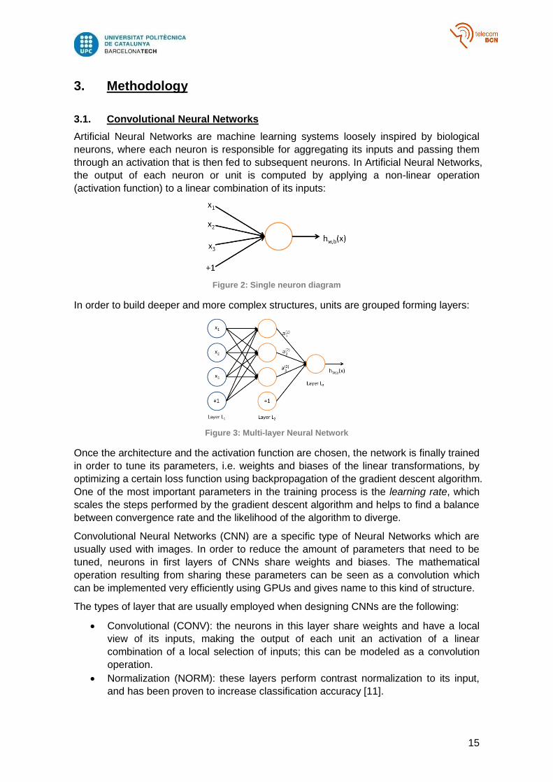
Artificial Neural Networks are machine learning systems loosely inspired by biological
neurons, where each neuron is responsible for aggregating its inputs and passing them
through an activation that is then fed to subsequent neurons. In Artificial Neural Networks,
the output of each neuron or unit is computed by applying a non-linear operation
(activation function) to a linear combination of its inputs:
Figure 2: Single neuron diagram
In order to build deeper and more complex structures, units are grouped forming layers:
Figure 3: Multi-layer Neural Network
Once the architecture and the activation function are chosen, the network is finally trained
in order to tune its parameters, i.e. weights and biases of the linear transformations, by
optimizing a certain loss function using backpropagation of the gradient descent algorithm.
One of the most important parameters in the training process is the learning rate, which
scales the steps performed by the gradient descent algorithm and helps to find a balance
between convergence rate and the likelihood of the algorithm to diverge.
Convolutional Neural Networks (CNN) are a specific type of Neural Networks which are
usually used with images. In order to reduce the amount of parameters that need to be
tuned, neurons in first layers of CNNs share weights and biases. The mathematical
operation resulting from sharing these parameters can be seen as a convolution which
can be implemented very efficiently using GPUs and gives name to this kind of structure.
The types of layer that are usually employed when designing CNNs are the following:
Convolutional (CONV): the neurons in this layer share weights and have a local
view of its inputs, making the output of each unit an activation of a linear
combination of a local selection of inputs; this can be modeled as a convolution
operation.
Normalization (NORM): these layers perform contrast normalization to its input,
and has been proven to increase classification accuracy [11].
16
Pooling (POOL): the goal of these layers is to perform a dimensionality reduction
by applying a pooling operation, i.e. max pooling, average pooling.
Fully Connected (FC): this layer connect every input to every neuron in the layer,
effectively making the output of each unit an activation of the linear combination of
all inputs; they are usually placed at the end of a network architecture.
Softmax: this layer is almost always placed on top of the architecture; the output
values of the last layer are converted into probabilities by applying the Softmax
transformation.
3.2. K-fold cross-validation
This is a common methodology in pattern classification that allows obtaining more
significant statistics, especially when working with small datasets. It consists of dividing
the dataset in K groups, or “folds,” and then using K-1 groups for training and the
remaining one for testing. The final result is obtained by repeating the former procedure K
times (so that each fold is used once as test data) and finally performing an average
operation.
3.3. Experimental setup
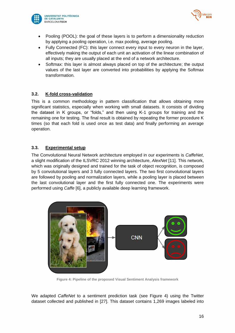
The Convolutional Neural Network architecture employed in our experiments is CaffeNet,
a slight modification of the ILSVRC 2012 winning architecture, AlexNet [11]. This network,
which was originally designed and trained for the task of object recognition, is composed
by 5 convolutional layers and 3 fully connected layers. The two first convolutional layers
are followed by pooling and normalization layers, while a pooling layer is placed between
the last convolutional layer and the first fully connected one. The experiments were
performed using Caffe [6], a publicly available deep learning framework.
Figure 4: Pipeline of the proposed Visual Sentiment Analysis framework
We adapted CaffeNet to a sentiment prediction task (see Figure 4) using the Twitter
dataset collected and published in [27]. This dataset contains 1,269 images labeled into
17
positive or negative by 5 different annotators. The choice was made based on the fact
that images in Twitter dataset are labeled by human annotators, oppositely to other
annotation methods which rely on textual tags or predefined concepts. Due to this fact,
the Twitter dataset is less noisy and allows the models to learn stronger concepts related
to the sentiment that an image provokes to a human. Given the subjective nature of
sentiment, different subsets can be formed depending on the number of annotators that
agreed on their decision. Only images that built consensus among all the annotators (5-
agree subset) were considered in our experiments. The resulting dataset is formed by
880 images (580 positive, 301 negative), which was later divided in 5 different folds to
evaluate experiments using cross-validation.
Each of the following subsections is self-contained and describes a different set of
experiments. Although the training conditions for all the experiments were defined as
similar as possible for the sake of comparison, there might be slight differences given
each individual experimental setup. For this reason, every section contains the
experiment description and its training conditions as well.
3.3.1. Fine-tuning CaffeNet
The adopted CaffeNet [6] architecture contains more than 60 million parameters, a figure
too high for training the network from scratch with the limited amount of data available in
the Twitter dataset. Given the good results achieved by previous works about transfer
learning [16], [20], we decided to explore the possibility of fine-tuning an already existing
model. Fine-tuning consists in initializing the weights in each layer but the last one with
those values learned from another model. The last layer is then replaced by a new one,
usually containing the same amount of neurons as classes in the dataset, and setting
random weights to this last layer. The advantage of this procedure compared to a random
initialization of all the network weights is that the gradient descent algorithm starting point
is much closer to an optimum, reducing both the amount of iterations needed before the
algorithm converges and the likelihood of overfitting when training with small datasets.
In the addressed problem of sentiment analysis, the last layer from the original architecture, fc8, is replaced by a new one composed of 2 neurons, one for positive and another for negative sentiment. The model of CaffeNet trained using ILSVRC 2012 dataset is used to initialize the rest of parameters in the network for the fine-tuning experiment. As the results are evaluated using 5-fold cross-validation, five different models of the same architecture need to be trained (one for each training set). They are all fine-tuned during 65 epochs (that is, every training image is fed 65 times into the CNN), with an initial base learning rate of 0.001 that is divided by 10 every 6 epochs. As the weights in the last layer are the only ones which are randomly initialized, its learning rate is set to be 10 times higher than the base learning rate in order to provide a faster convergence rate.
A common practice when working with CNNs is data augmentation, which consists in
generating different versions of each image by applying simple transformations such as
flips and crops. Recent work has proved that this technique reports a consistent
improvement in accuracy [2], so we decided to explore whether data augmentation
improves the spatial generalization capability of our system by feeding 10 different
combination of flips and crops of the original image to the network in the test stage. The
classification scores obtained for each combination are finally fused with an averaging
operation.
18
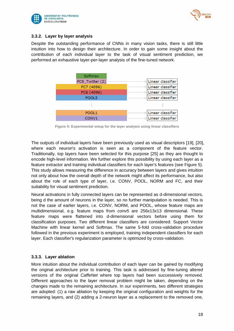
3.3.2. Layer by layer analysis
Despite the outstanding performance of CNNs in many vision tasks, there is still little
intuition into how to design their architecture. In order to gain some insight about the
contribution of each individual layer to the task of visual sentiment prediction, we
performed an exhaustive layer-per-layer analysis of the fine-tuned network.
Figure 5: Experimental setup for the layer analysis using linear classifiers
The outputs of individual layers have been previously used as visual descriptors [19], [20],
where each neuron's activation is seen as a component of the feature vector.
Traditionally, top layers have been selected for this purpose [25] as they are thought to
encode high-level information. We further explore this possibility by using each layer as a
feature extractor and training individual classifiers for each layer's features (see Figure 5).
This study allows measuring the difference in accuracy between layers and gives intuition
not only about how the overall depth of the network might affect its performance, but also
about the role of each type of layer, i.e. CONV, POOL, NORM and FC, and their
suitability for visual sentiment prediction.
Neural activations in fully connected layers can be represented as d-dimensional vectors,
being d the amount of neurons in the layer, so no further manipulation is needed. This is
not the case of earlier layers, i.e. CONV, NORM, and POOL, whose feature maps are
multidimensional, e.g. feature maps from conv5 are 256x13x13 dimensional. These
feature maps were flattened into d-dimensional vectors before using them for
classification purposes. Two different linear classifiers are considered: Support Vector
Machine with linear kernel and Softmax. The same 5-fold cross-validation procedure
followed in the previous experiment is employed, training independent classifiers for each
layer. Each classifier's regularization parameter is optimized by cross-validation.
3.3.3. Layer ablation
More intuition about the individual contribution of each layer can be gained by modifying
the original architecture prior to training. This task is addressed by fine-tuning altered
versions of the original CaffeNet where top layers had been successively removed.
Different approaches to the layer removal problem might be taken, depending on the
changes made to the remaining architecture. In our experiments, two different strategies
are adopted: (1) a raw ablation by keeping the original configuration and weights for the
remaining layers, and (2) adding a 2-neuron layer as a replacement to the removed one,
19
on top of the remaining architecture and just before the Softmax layer. A more detailed
definition of the experimental setup for each configuration is described in the following
subsections.
Figure 6: Layer ablation architectures
3.3.3.1. Raw ablation
In this set of experiments, the Softmax layer is placed on top of the remaining
architecture, e.g. if fc8 and fc7 are removed, the output of fc6 is connected to the input of
the Softmax layer. Weights from the original model are kept as well. The configurations
studied in our experiments include versions of CaffeNet where (1) fc8 has been ablated,
and (2) both fc8 and fc7 have been removed (architectures fc7-4096 and fc6-4096,
respectively, in Figure 6). The models are trained during 65 epochs, with a base learning
rate of 0.001 that is divided by 10 every 6 epochs. With this configuration all the weights
are initialized using the pre-trained model, so random initialization of parameters is not
necessary. Given this fact, there is no need to increase the individual learning rate of any
layer.
3.3.3.2. 2-neuron on top
As described in Section 3.3.1, fine-tuning consists in replacing the last layer in a net by a
new one and using the weights in a pre-trained model as initialization for the rest of layers.
Inspired by this procedure, we decided to combine the former methodology with the layer
removal experiments: instead of leaving the whole remaining architecture unmodified
after a layer is removed, its last remaining layer is replaced by a 2-neuron layer with
random initialization of the weights. This set of experiments comprises the fine-tuning of
modified versions of CaffeNet where (1) fc8 has been removed and fc7 has been
replaced by a 2-neuron layer, and (2) fc8 and fc7 have been ablated and fc6 has been
replaced by a 2-neuron layer (architectures fc7-2 and fc6-2, respectively, in Figure 6).
The models are trained during 65 epochs, dividing the base learning rate by 10 every 6
epochs and with a learning rate 10 times higher than the base one for the 2-neuron layer,
as its weights are being randomly initialized. The base learning rate of the former
configuration is 0.001, while the latter's was set to 0.0001 to avoid divergence.
3.3.4. Layer addition
None of the architectures that have been introduced so far take into account the
information encoded in the last layer (fc8) of the original CaffeNet model. This layer
contains a confidence value for the image belonging to each one of the 1,000 classes in
ILSVRC 2012. In addition, fully connected layers contain, by far, most of the parameters
in a Convolutional Neural Network. Therefore, from both of the former points of view, a
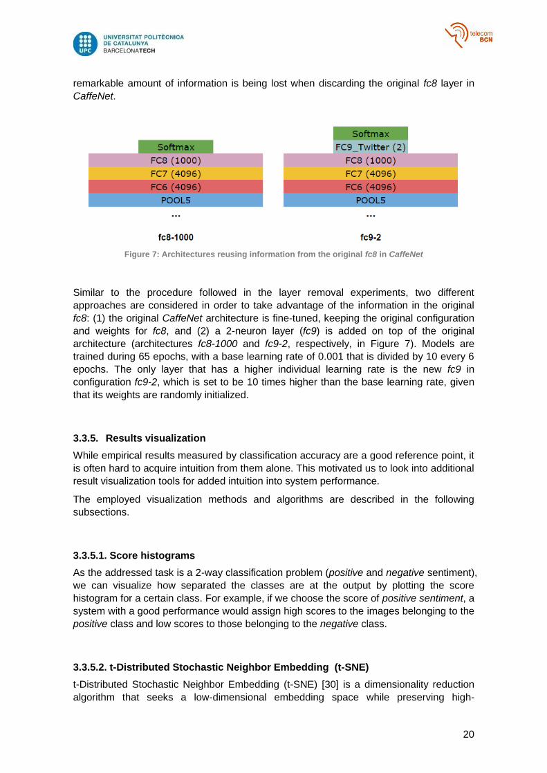
20
remarkable amount of information is being lost when discarding the original fc8 layer in
CaffeNet.
Figure 7: Architectures reusing information from the original fc8 in CaffeNet
Similar to the procedure followed in the layer removal experiments, two different
approaches are considered in order to take advantage of the information in the original
fc8: (1) the original CaffeNet architecture is fine-tuned, keeping the original configuration
and weights for fc8, and (2) a 2-neuron layer (fc9) is added on top of the original
architecture (architectures fc8-1000 and fc9-2, respectively, in Figure 7). Models are
trained during 65 epochs, with a base learning rate of 0.001 that is divided by 10 every 6
epochs. The only layer that has a higher individual learning rate is the new fc9 in
configuration fc9-2, which is set to be 10 times higher than the base learning rate, given
that its weights are randomly initialized.
3.3.5. Results visualization
While empirical results measured by classification accuracy are a good reference point, it
is often hard to acquire intuition from them alone. This motivated us to look into additional
result visualization tools for added intuition into system performance.
The employed visualization methods and algorithms are described in the following
subsections.
3.3.5.1. Score histograms
As the addressed task is a 2-way classification problem (positive and negative sentiment),
we can visualize how separated the classes are at the output by plotting the score
histogram for a certain class. For example, if we choose the score of positive sentiment, a
system with a good performance would assign high scores to the images belonging to the
positive class and low scores to those belonging to the negative class.
3.3.5.2. t-Distributed Stochastic Neighbor Embedding (t-SNE)
t-Distributed Stochastic Neighbor Embedding (t-SNE) [30] is a dimensionality reduction
algorithm that seeks a low-dimensional embedding space while preserving high-
21
dimensional distance information. This representation has become particular popular in
the deep learning community as a visualization tool.
3.3.5.3. Top-K scores
By visualizing the top-K images that produce the highest score for each class it is
possible to gain some intuition about which elements or visual features are associated
with each sentiment in the network.
3.3.5.4. Receptive fields
The concept of a receptive field is exploited in [29] to visualize which parts of an image
activate certain neuronal units. With this visualization, they conclude that they are better
able to visualize patterns discovered by deep networks, e.g. starting with edges or
textures in the first layers and ending with parts of objects or even complete objects in the
highest layers.
This kind of visualization, unlike previous ones, allows us to better understand the
behavior of individual units in the CNN with respect to the original input image space.
22
4. Results
This section presents the results for the experiments proposed in Section 3.3, as well as
intuition and conclusions.
4.1. Evaluation metric: Accuracy
Accuracy is the evaluation metric employed in our experiments, and is defined by the
following equation:
𝐴𝑐𝑐𝑢𝑟𝑎𝑐𝑦 = 𝑛𝑢𝑚𝑏𝑒𝑟 𝑜𝑓 𝑐𝑜𝑟𝑟𝑒𝑐𝑡𝑙𝑦 𝑝𝑟𝑒𝑑𝑖𝑐𝑡𝑒𝑑 𝑠𝑎𝑚𝑝𝑙𝑒𝑠
𝑛𝑢𝑚𝑏𝑒𝑟 𝑜𝑓 𝑠𝑎𝑚𝑝𝑙𝑒𝑠
4.2. Fine-tuning CaffeNet
Average accuracy results over the 5 folds for the fine-tuning experiment are presented in Table 1, which also includes the results for the best fine-tuned model in [27]. This CNN, with a 2CONV-4FC architecture, was designed specifically for visual sentiment prediction and trained using almost half million sentiment annotated images from Flickr dataset [1]. The network was finally fine-tuned on the Twitter 5-agree dataset with a resulting accuracy of 0.783 which is, to best of our knowledge, the best result on this dataset so far.
Model Accuracy
Fine-tuned CNN from You et al. [27] 0.783
Fine-tuned CaffeNet 0.817 ± 0.038
Fine-tuned CaffeNet with oversampling 0.830 ± 0.034
Table 1: 5-fold cross-validation results on 5-agree Twitter dataset
Surprisingly, fine-tuning a net that was originally trained for object recognition reported higher accuracy in visual sentiment prediction than a CNN that was specifically trained for that task. On one hand, this fact suggests the importance of high-level representations such as semantics in visual sentiment prediction, as transferring learning from object recognition to sentiment analysis actually generates high accuracy rates. On the other hand, it seems that visual sentiment prediction architectures also benefit from a higher amount of convolutional layers, as suggested by [28] for the task of object recognition.
Averaging the prediction over modified versions of the input image (oversampling) results in a consistent improvement in the prediction accuracy. This behavior, which was already observed by the authors of [2] when addressing the task of object recognition, suggests that the former procedure also increases the network's generalization capability for visual sentiment analysis, as the final prediction is far less dependent on the spatial distribution of the input image.
23
4.3. Layer by layer analysis
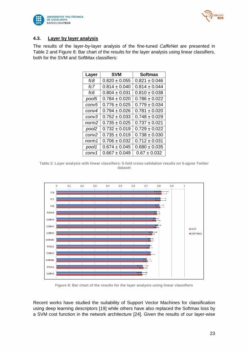
The results of the layer-by-layer analysis of the fine-tuned CaffeNet are presented in
Table 2 and Figure 8: Bar chart of the results for the layer analysis using linear classifiers,
both for the SVM and SoftMax classifiers:
Layer SVM Softmax
fc8 0.820 ± 0.055 0.821 ± 0.046
fc7 0.814 ± 0.040 0.814 ± 0.044
fc6 0.804 ± 0.031 0.810 ± 0.038
pool5 0.784 ± 0.020 0.786 ± 0.022
conv5 0.776 ± 0.025 0.779 ± 0.034
conv4 0.794 ± 0.026 0.781 ± 0.020
conv3 0.752 ± 0.033 0.748 ± 0.029
norm2 0.735 ± 0.025 0.737 ± 0.021
pool2 0.732 ± 0.019 0.729 ± 0.022
conv2 0.735 ± 0.019 0.738 ± 0.030
norm1 0.706 ± 0.032 0.712 ± 0.031
pool1 0.674 ± 0.045 0.680 ± 0.035
conv1 0.667 ± 0.049 0.67 ± 0.032
Table 2: Layer analysis with linear classifiers: 5-fold cross-validation results on 5-agree Twitter dataset
Figure 8: Bar chart of the results for the layer analysis using linear classifiers
Recent works have studied the suitability of Support Vector Machines for classification
using deep learning descriptors [19] while others have also replaced the Softmax loss by
a SVM cost function in the network architecture [24]. Given the results of our layer-wise
24
analysis, it is not possible to claim that any of the two classifiers provides a consistent
gain compared to the other for visual sentiment analysis, at least, in the Twitter 5-agree
dataset with the proposed network architecture.
Accuracy trends at each layer reveal that the depth of the networks contributes to the
increase of performance. Not every single layer produces an increase in accuracy with
respect to the previous one, but even in those stages it is hard to claim that the
architecture should be modified as higher layers might be benefiting from its effect, e.g.
conv5 and pool5 report lower accuracy rates than earlier conv4 when their feature maps
are used for classification, but later fully connected layers might be benefiting from the
effect of conv5 and pool5 as all of them report higher accuracy than conv4.
An increase in performance is observed with each fully connected layer, as every stage
introduces some gain with respect to the previous one. This fact suggests that adding
additional fully connected layers might report even higher accuracy rates, but further
research is necessary to evaluate this hypothesis.
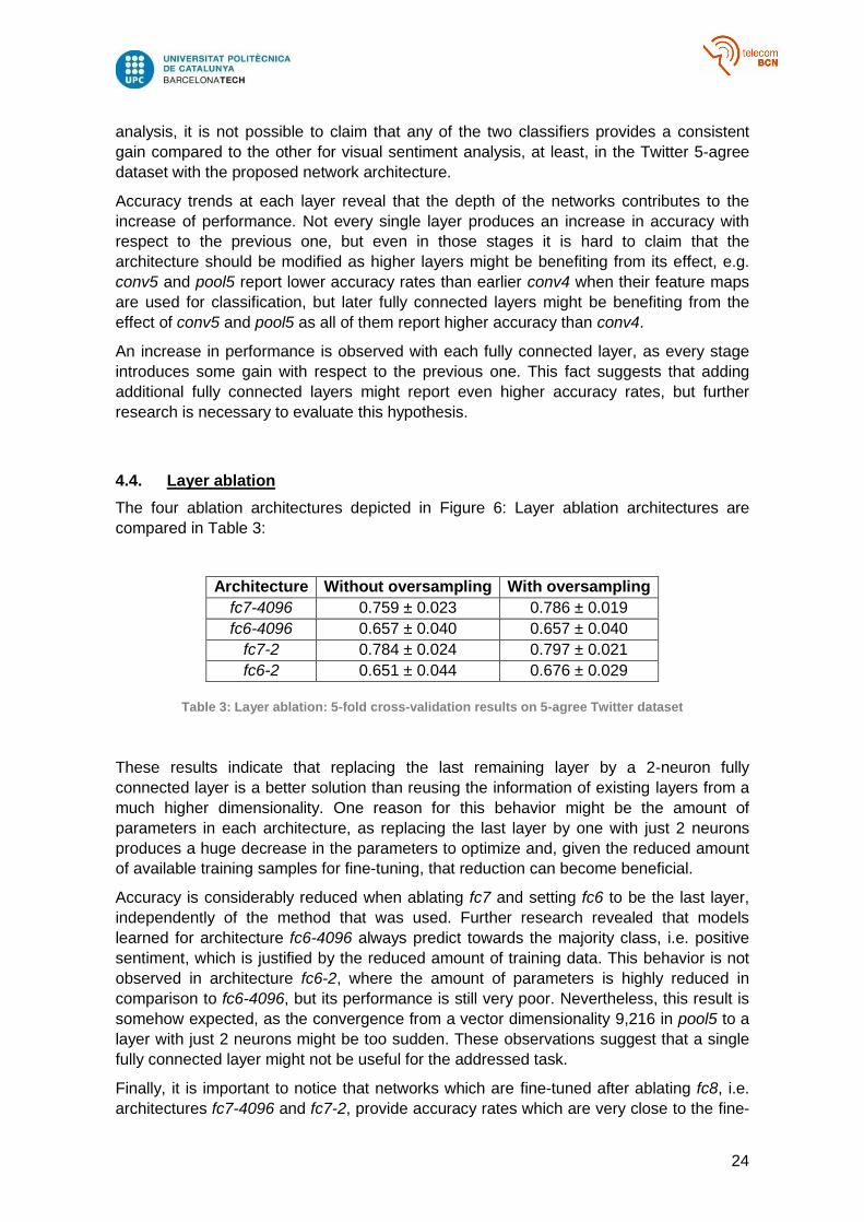
4.4. Layer ablation
The four ablation architectures depicted in Figure 6: Layer ablation architectures are
compared in Table 3:
Architecture Without oversampling With oversampling
fc7-4096 0.759 ± 0.023 0.786 ± 0.019
fc6-4096 0.657 ± 0.040 0.657 ± 0.040
fc7-2 0.784 ± 0.024 0.797 ± 0.021
fc6-2 0.651 ± 0.044 0.676 ± 0.029
Table 3: Layer ablation: 5-fold cross-validation results on 5-agree Twitter dataset
These results indicate that replacing the last remaining layer by a 2-neuron fully
connected layer is a better solution than reusing the information of existing layers from a
much higher dimensionality. One reason for this behavior might be the amount of
parameters in each architecture, as replacing the last layer by one with just 2 neurons
produces a huge decrease in the parameters to optimize and, given the reduced amount
of available training samples for fine-tuning, that reduction can become beneficial.
Accuracy is considerably reduced when ablating fc7 and setting fc6 to be the last layer,
independently of the method that was used. Further research revealed that models
learned for architecture fc6-4096 always predict towards the majority class, i.e. positive
sentiment, which is justified by the reduced amount of training data. This behavior is not
observed in architecture fc6-2, where the amount of parameters is highly reduced in
comparison to fc6-4096, but its performance is still very poor. Nevertheless, this result is
somehow expected, as the convergence from a vector dimensionality 9,216 in pool5 to a
layer with just 2 neurons might be too sudden. These observations suggest that a single
fully connected layer might not be useful for the addressed task.
Finally, it is important to notice that networks which are fine-tuned after ablating fc8, i.e.
architectures fc7-4096 and fc7-2, provide accuracy rates which are very close to the fine-
25
tuned CNN in [27] or even higher. These results, as shown by the authors in [28] for the
task of object recognition, suggest that removing one of the fully connected layers (and
with it, a high percentage of the parameters in the architecture) only produces a slight
deterioration in performance, but the huge decrease in the parameters to optimize might
allow the use of smaller datasets without overfitting the model. This is a very interesting
result for visual sentiment prediction given the complexity of obtaining reliable annotated
images for such task.
4.5. Layer addition
The architectures that keep fc8 are evaluated in Table 4, indicating that architecture fc9-2
outperforms fc8-1000. This observation, together with the previous in Section 4.4,
strengthens the thesis that CNNs deliver a higher performance in classification tasks
when the last layer contains one neuron for each class.
Architecture Without oversampling With oversampling
fc8-1000 0.723 ± 0.041 0.731 ± 0.036
fc9-2 0.795 ± 0.023 0.803 ± 0.034
Table 4: Layer addition: 5-fold cross-validation results on 5-agree Twitter dataset
The best accuracy results when reusing information from the original fc8 are obtained by
adding a new layer, fc9, although they are slightly worse than those obtained with the
regular fine-tuning (Table 1). At first sight, this observation may seem contrary to intuition
gained in the layer-wise analysis, which suggested that a deeper architecture would have
a better performance. If a holistic view is taken and not only the network architecture is
considered, we observe that including information from the 1,000 classes in ILSVRC
2012 (e.g. zebra, library, red wine) may not help in sentiment prediction, as they are
mainly neutral or do not provide any sentimental cues without contextual information.
The reduction in performance when introducing semantic concepts that are neutral with
respect to sentiment, together with the results in Section 4.3, highlights the importance of
appropriate mid-level representation such as the Visual Sentiment Ontology built in [1]
when addressing the task of visual sentiment prediction. Nevertheless, they suggest that
generic features such as neural codes in fc7 outperform semantic representations when
the latter are not sentiment specific. This intuition meets the results in [25], where the
authors found out that training a classifier using CaffeNet’s fc7 instead of fc8 reported
better performance for the task of visual sentiment prediction.
4.6. Results visualization
4.6.1. Score histograms
Empirical results from the previous experiments show a reduction in accuracy when
removing layers and even when adding the new fc9. This behavior can also be observed
by comparing the score histograms for each network architecture as classes become less

26
separated. Figure 9 and Figure 10 demonstrate this statement by depicting the score
histograms the CNN with the regular fine-tuning (best performance) and for the ablated
architecture fc6-2 (poor performance).
Figure 9: Score histogram for the regular fine-tuning
Figure 10: Score histogram for architecture fc6-2
4.6.2. t-Distributed Stochastic Neighbor Embedding (t-SNE)
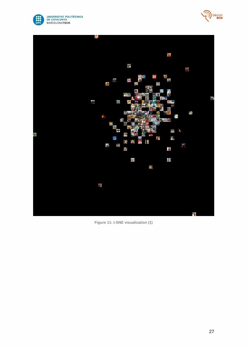
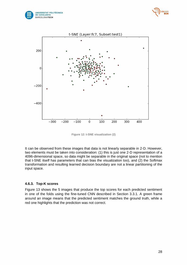
The following figures show the t-SNE representation for the first fold using fc7 layer from the fine-tuned network described in Section 3.3.1. While Figure 11 contains thumbnails of the images, Figure 12 contains their ground truth (where green dots represent positive images and red dots, negative images):
Positive sentiment score
Positive sentiment score
27
Figure 11: t-SNE visualization (1)
28
Figure 12: t-SNE visualization (2)
It can be observed from these images that data is not linearly separable in 2-D. However, two elements must be taken into consideration: (1) this is just one 2-D representation of a 4096-dimensional space, so data might be separable in the original space (not to mention that t-SNE itself has parameters that can bias the visualization too), and (2) the Softmax transformation and resulting learned decision boundary are not a linear partitioning of the input space.
4.6.3. Top-K scores
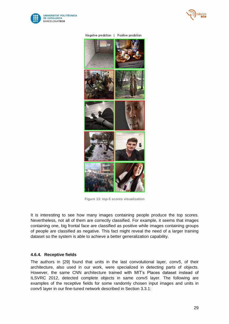
Figure 13 shows the 5 images that produce the top scores for each predicted sentiment
in one of the folds using the fine-tuned CNN described in Section 3.3.1. A green frame
around an image means that the predicted sentiment matches the ground truth, while a
red one highlights that the prediction was not correct.
29
Figure 13: top-5 scores visualization
It is interesting to see how many images containing people produce the top scores.
Nevertheless, not all of them are correctly classified. For example, it seems that images
containing one, big frontal face are classified as positive while images containing groups
of people are classified as negative. This fact might reveal the need of a larger training
dataset so the system is able to achieve a better generalization capability.
4.6.4. Receptive fields
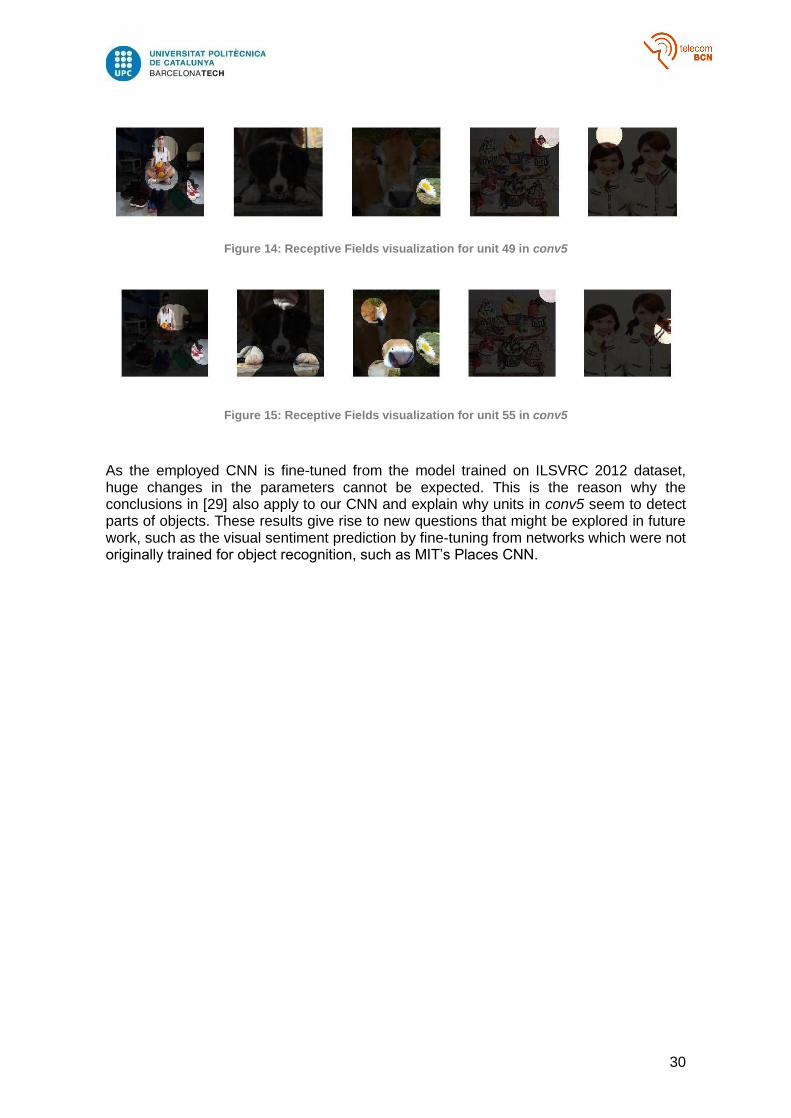
The authors in [29] found that units in the last convolutional layer, conv5, of their
architecture, also used in our work, were specialized in detecting parts of objects.
However, the same CNN architecture trained with MIT’s Places dataset instead of
ILSVRC 2012, detected complete objects in same conv5 layer. The following are
examples of the receptive fields for some randomly chosen input images and units in
conv5 layer in our fine-tuned network described in Section 3.3.1:
30
Figure 14: Receptive Fields visualization for unit 49 in conv5
Figure 15: Receptive Fields visualization for unit 55 in conv5
As the employed CNN is fine-tuned from the model trained on ILSVRC 2012 dataset, huge changes in the parameters cannot be expected. This is the reason why the conclusions in [29] also apply to our CNN and explain why units in conv5 seem to detect parts of objects. These results give rise to new questions that might be explored in future work, such as the visual sentiment prediction by fine-tuning from networks which were not originally trained for object recognition, such as MIT’s Places CNN.

31
5. Budget
This research project has been developed using open source software, so its cost mainly comes in the shape of the time spent by the researchers involved in it:
Amount Wage Hours spent Total
Junior engineer 1 8.00€/h 360h 2,880€
Senior engineer 3 20.00€/h 60h 3,600€
TOTAL: 6,480€

32
6. Conclusions and future work
We presented several experiments studying the suitability of fine-tuned CNNs for the task
of visual sentiment prediction. We showed the utility of deep architectures that are
capable of capturing high level features when addressing the former task, obtaining
models that outperform the best results so far in the evaluation dataset. Data
augmentation has been demonstrated to be a useful technique for increasing visual
sentiment prediction accuracy as well. Our study of domain transfer from object
recognition to sentiment analysis has reinforced common good practices in the field:
discarding the last fully connected layer adapted to another task, and the addition of a
new randomly initialized layer with as many neurons as the amount of categories to
classify.
The layer-wise analysis both with linear classifiers and modified architectures has shown
the importance of the depth in CNNs when addressing tasks that require a high
abstraction level, such as visual sentiment prediction.
Future work will compare between entirely different architectures, in addition to modified
versions of the same network, and the expansion of the presented experiments to CNNs
which are trained from scratch for the task of visual sentiment prediction. Nevertheless,
the previous task arises new problems such as the generation of huge sentiment
annotated datasets, which may be noisy given the subjective nature of perceived
sentiment, and the reduction and handling of such noise when training new models.
Finally, the work reported in this thesis is the core contribution of a scientific publication
under progress co-authored with my three advisors. This paper will be submitted to the
Affect and Sentiment in Multimedia (ASM) workshop, to be held in conjunction of the
ACM Multimedia Conference 2015 in Brisbane, Australia.
33
Bibliography:
[1] BORTH, D.; JI, R.; CHEN, T.; BREUEL, T. & CHANG, S.-F.: Large-scale Visual Sentiment Ontology and Detectors Using Adjective Noun Pairs. In: ACM MM., 2013
[2] CHATFIELD, K.; SIMONYAN, K.; VEDALDI, A. & ZISSERMAN, A.: Return of the Devil in the Details: Delving Deep into Convolutional Nets. In: British Machine Vision Conference., 2014
[3] DENG, J.; DONG, W.; SOCHER, R.; LI, L.-J.; LI, K. & FEI-FEI, L.: ImageNet: A large-scale hierarchical image database. In: Computer Vision and Pattern Recognition, 2009. CVPR 2009. IEEE Conference on., 2009, S. 248--255
[4] HE, K.; ZHANG, X.; REN, S. & SUN, J.: Delving Deep into Rectifiers: Surpassing Human-Level Performance on ImageNet Classification. In: arXiv:abs/1502.01852 [cs.CV] (2015)
[5] JIA, J.; WU, S.; WANG, X.; HU, P.; CAI, L. & TANG, J.: Can We Understand van Gogh's mood?: Learning to Infer Affects from Images in Social Networks. In:ACM MM., 2012
[6] JIA, Y.; SHELHAMER, E.; DONAHUE, J.; KARAYEV, S.; LONG, J.; GIRSHICK, R.; GUADARRAMA, S. & DARRELL, T.: Caffe: Convolutional Architecture for Fast Feature Embedding. In:ACM MM., 2014
[7] JIANG, Y.-G.; XU, B. & XUE, X.: Predicting Emotions in User-Generated Videos. In: AAAI., 2014
[8] JIN, X.; GALLAGHER, A.; CAO, L.; LUO, J. & HAN, J.: The Wisdom of Social Multimedia: Using Flickr for Prediction and Forecast. In: ACM MM., 2010
[9] JOU, B.; BHATTACHARYA, S. & CHANG, S.-F.: Predicting Viewer Perceived Emotions in Animated GIFs. In: ACM MM., 2014
[10] KIM, Y.; LEE, H. & PROVOST, E. M.: Deep learning for robust feature generation in audiovisual emotion recognition. In: ICASSP., 2013
[11] KRIZHEVSKY, A.; SUTSKEVER, I. & HINTON, G. E.: ImageNet Classification with Deep Convolutional Neural Networks. In: NIPS., 2012
[12] LANG, P.; BRADLEY, M. & CUTHBERT, B.: International Affective Picture System (IAPS): Technical Manual and Affective Ratings, Bericht, NIMH CSEA, 1997
[13] LECUN, Y.; BOTTOU, L.; BENGIO, Y. & HAFFNER, P.: Gradient-based Learning Applied to Document Recognition. In: Proc. of the IEEE., 1998
[14] MACHAJDIK, J. & HANBURY, A.: Affective Image Classification Using Features Inspired by Psychology and Art Theory. In: ACM MM., 2010
[15] MCDUFF, D.; KALIOUBY, R.; COHN, J. & PICARD, R.: Predicting Ad Liking and Purchase Intent: Large-scale Analysis of Facial Responses to Ads., 2014
[16] OQUAB, M.; BOTTOU, L.; LAPTEV, I. & SIVIC, J.: Learning and transferring mid-level image representations using convolutional neural networks. In: Computer Vision and Pattern Recognition (CVPR), 2014 IEEE Conference on., 2014, S. 1717--1724
[17] PENG, K.-C.; CHEN, T.; SADOVNIK, A. & GALLAGHER, A.: A Mixed Bag of Emotions: Model, Predict, and Transfer Emotion Distributions. In: CVPR., 2015
[18] PLUTCHIK, R.: Emotion: A Psychoevolutionary Synthesis: Harper & Row., 1980
[19] RAZAVIAN, A. S.; AZIZPOUR, H.; SULLIVAN, J. & CARLSSON, S.: CNN Features off-the-shelf: An Astounding Baseline for Recognition. In: Computer Vision and Pattern Recognition Workshops (CVPRW), 2014 IEEE Conference on., 2014, S. 512--519
[20] SALVADOR, A.; ZEPPELZAUER, M.; MANCHON-VIZUETE, D.; CALAFELL, A. & GIRO-I-NIETO, X.: Cultural Event Recognition with Visual ConvNets and Temporal Models. In: Computer Vision and Pattern Recognition Workshops (CVPRW), 2015 IEEE Conference on., 2015
[21] SIERSDORFER, S.; MINACK, E.; DENG, F. & HARE, J.: Analyzing and predicting sentiment of images on the social web. In:Proceedings of the international conference on Multimedia., 2010, S. 715--718
[22] SZEGEDY, C.; LIU, W.; JIA, Y.; SERMANET, P.; REED, S.; ANGUELOV, D.; ERHAN, D.; VANHOUCKE, V. &
RABINOVICH, A.: Going deeper with convolutions. In: arXiv preprint arXiv:1409.4842 (2014)
[23] SZEGEDY, C.; ZAREMBA, W.; SUTSKEVER, I.; BRUNA, J.; ERHAN, D.; GOODFELLOW, I. & FERGUS, R.: Intriguing properties of neural networks. In: ICLR., 2014
[24] TANG, Y.: Deep Learning using Linear Support Vector Machines. In: ICML Workshop on Challenges in Representation Learning., 2013
[25] XU, C.; CETINTAS, S.; LEE, K.-C. & LI, L.-J.: Visual Sentiment Prediction with Deep Convolutional Neural Networks. In: arXiv preprint arXiv:1411.5731 (2014)

34
[26] YANULEVSKAYA, V.; VAN GEMERT, J.; ROTH, K.; HERBOLD, A.; SEBE, N. & GEUSEBROEK, J. M.: Emotional Valence Categorization Using Holistic Image Features. In: ICIP., 2008
[27] YOU, Q.; LUO, J.; JIN, H. & YANG, J.: Robust Image Sentiment Analysis using Progressively Trained and Domain Transferred Deep Networks. In: The Twenty-Ninth AAAI Conference on Artificial Intelligence (AAAI)., 2015
[28] ZEILER, M. D. & FERGUS, R.: Visualizing and understanding convolutional networks: Springer. : Computer Vision–ECCV 2014., 2014, S. 818--833
[29] ZHOU, B.; KHOSLA, A.; LAPEDRIZA, A.; OLIVA, A. & TORRALBA, A.: Object detectors emerge in deep scene cnns. In: (2015)
[30] VAN DER MAATEN, LAURENS; HINTON, GEOFFREY. Visualizing data using t-SNE. Journal of Machine Learning Research, 2008, vol. 9, no 2579-2605, p. 85.

35
Appendix 1: Work packages
Documentation WP ref: WP1
Major constituent: Documentation Sheet 1 of 6
Short description:
Develop the different documents that describe the
project and its development
Planned start date:
16/02/2015
Planned end date: 10/07/2015
Start event: Project start
End event: Final report
submission
T1: Project planning
T2: Work plan redaction
T3: Work plan revision
T4: Work plan approval
T5: Critical Design Review redaction
T6: Critical Design Review revision
T7: Critical Design Review approval
T8: Final report redaction
T9: Final report revision
T10: Final report approval
T11: Scientific publication with the results from the
project
Deliverables:
Work plan
CDR
Final Report
Paper
submission
Dates:
27/02/2015
24/04/2015
10/07/2015
13/07/2015
State of the art WP ref: WP2
Major constituent: Documentation Sheet 2 of 6
Short description:
Study and understand the state of the art solutions in the
fields of deep learning and affective computing related to
computer vision
Planned start date:
02/02/2015
Planned end date:
10/07/2015
Start event: Project start
End event: -
T1: Understanding the state of the art for deep learning Deliverables: Dates:
36
T2: Understanding the state of the art for affective
computing
T3: Keeping an eye on new publications about deep
learning applied to the field of affective computing
Software WP ref: WP3
Major constituent: Software Sheet 3 of 6
Short description:
This package includes getting used to the software tools
used during the project and all the scripting that needs to
be done to perform the experiments
Planned start date:
09/02/2015
Planned end date:
10/07/2015
Start event: Project start
End event: -
T1: Learning how to work with GPI’s servers
T2: Understanding how to use Caffe’s Python wrapper
T3: Learning how to work with files and numpy arrays
using Python
T4: Developing the scripts needed for the experiments
T5: Submitting the code to GPI’s git repository
Deliverables:
Code
submission
Dates:
15/07/2015
Datasets WP ref: WP4
Major constituent: Data obtaining Sheet 4 of 6
Short description:
Finding suitable datasets for the experiments and
obtaining them.
Planned start date:
09/02/2015
Planned end date:
24/04/2015
Start event: 1st Meeting with
Brendan
End event: -
T1: Get IAPS dataset
T2: Get Twitter dataset
Deliverables: Dates:
37
T3: Get Flickr dataset
Experiments WP ref: WP5
Major constituent: Experimentation and Results
evaluation
Sheet 5 of 6
Short description:
Designing and performing experiments in the field of
affective computing using deep learning.
Planned start date:
09/02/2015
Planned end date:
24/06/2015
Start event: 1st Meeting with
Brendan
End event: -
T1: Arousal/valence prediction on IAPS dataset
T2: Results evaluation of the experiment on IAPS dataset
T3: Fine-tuning CaffeNet using Twitter Dataset
T4: Results evaluation of the fine-tuning of Caffenet
using Twitter Dataset experiment
T5: Training a CNN on Flickr dataset using a state of the
art network architecture
T6: Results evaluation of training a CNN on Flickr
dataset using a state of the art network architecture
experiment
T7: Training classifiers on top of each layer of CaffeNet
using Twitter dataset
T8: Removing layers from CaffeNet and fine-tuning the
new networks using Twitter dataset
T9: Assess results from the layer analysis experiments
T10: Results visualization
Deliverables: Dates:
Oral communication WP ref: WP6
Major constituent: Documentation Sheet 6 of 6
Short description:
Preparation of the thesis’ oral defense
Planned start date:
10/07/2015
Planned end date:

38
20/07/2015
Start event: Final report
approval
End event: Oral defense
T1: Preparing the support slides
T2: First rehearsal
T3: Second rehearsal
T4: Last modifications on the support slides
T5: Oral defense
Deliverables:
Slides
Dates:
39
Appendix 2: Complete Gantt diagram
Figure 16: Complete Gantt diagram

40
Glossary
CNN: Convolutional Neural Network
ILSVRC: Image Large Scale Visual Recognition Challenge
SVM: Support Vector Machine
t-SNE: t-Distributed Stochastic Neighbor Embedding