latin american beer production and import demand for
TRANSCRIPT

Latin American Beer Production and Import Demand for Regional Malt and Malted Barley
DOCUMENTO DE TRABAJO N° 85
Agosto de 2021
Red Nacional deInvestigadoresen Economía
Rodrigo García Arancibia (Universidad Nacional del Litoral/CONICET/RedNIE)
Mariano Coronel (Universidad Nacional del Litoral)
Jimena Vicentin Masaro (Universidad Nacional del Litoral / RedNIE)

Los documentos de trabajo de la RedNIE se difunden con el propósito degenerar comentarios y debate, no habiendo estado sujetos a revisión de pares.Las opiniones expresadas en este trabajo son de los autores y nonecesariamente representan las opiniones de la RedNIE o su ComisiónDirectiva.
The RedNIE working papers are disseminated for the purpose of generatingcomments and debate, and have not been subjected to peer review. Theopinions expressed in this paper are exclusively those of the authors and donot necessarily represent the opinions of the RedNIE or its Board of Directors.
Citar como:García Arancibia, Rodrigo, Mariano Coronel y Jimena Vicentin Masaro (2021).Latin American Beer Production and Import Demand for Regional Malt andMalted Barley. Documento de trabajo RedNIE N°85.

Latin American beer production and import demand for Regional
malt and malted barley∗
Rodrigo Garcıa Arancibia1,2,3, Mariano Coronel1, and Jimena Vicentin Masaro1,3
1Instituto de Economıa Aplicada Litoral (IECAL), FCE-Universidad Nacional del Litoral2Consejo Nacional de Investigaciones Cientıficas y Tecnologicas (CONICET, Argentina)
3RedNIE
Abstract
The Latin American beer sector has undergone important changes over the last 25 years.
The growth in beer production, consumption, and trade has been accompanied by a greater
demand for malt and barley produced and traded in the region, displacing other traditional
export countries of these inputs. Based on these facts, we studied the long-term relationship
between this increase in beer production and the prices of imported inputs. In addition, we
estimated the elaticities of demand of imported inputs of the main Latin American brewing
countries. This allow as to infer about Latin America’s competitive position as a supplier of its
own beer inputs.
Keywords: beer inputs; import demand; cointegration; demand elasticities; regional integration.
∗Acknowledgments: This work was supported by the Agencia Nacional de Promocion a la Investigacion, el De-
sarrollo Tecnologico y la Innovacion (Ministerio de Ciencia, Tecnologıa e Innovacion, Argentina) under Grant PICT
2018-04377. We thank Ana Laura Chara for her work as a research assistant, contributing to the data collection
and maps. Corresponding author: IECAL-FCE, Moreno 2557. S3000CVE - Santa Fe. Santa Fe. Argentina, e-mail:
1

1 Introduction
Important changes have occurred in the Latin American beer market over last twenty-five years.
These changes have occurred both from the point of view of production and consumption, with a
domestic market expansion in each particular country, as well as in regional and international trade.
Whereas the production and demand have stagnated in traditional regions, such as Europe, the
United States (US), and Canada, non-traditional ones have had a sustained growth in these items,
such as Latin America, Africa, and Asia (Swinnen, 2011). In fact, Latin America has overtaken
the US and Canada joint production since 2006, which is mainly explained by the increase in beer
production in Brazil and Mexico. Furthermore, Mexico has become the world’s leading exporter,
surpassing the main traditional beer exporters since 2010, such as the Netherlands, Belgium, and
Germany (Thome and Soares, 2015). So much so that in 2019 Mexican exports doubled those of
Netherlands, the second largest exporter in the world (WTEx, 2020).
Latin America has positioned itself as one of the main beer-consuming regions. In particular,
it is remarkable the case of Brazil, which together with China and the United States has become
one of the main beer markets in world (Swinnen and Briski, 2017). According to the World Health
Organization (WHO) consumption series, there are some common facts in the changes in alcohol
consumption patterns that can be highlighted (WHO, 2018). Specifically, while the amount of total
alcohol consumption is decreasing considering the last 30 years, the same is not true for beer, which
shows a growing trend. This shows a propensity of consumption in the region in favor of beer, to
the detriment of other beverages of habitual consumption like wine and spirits. In particular, in
those countries where wine consumption was traditionally predominant, such as Argentina, Chile,
and Uruguay, beer consumption has come to equal or exceed it. Similarly, in countries such as Peru,
Paraguay, Bolivia, and a large majority of the countries of Central America and the Caribbean,
where the consumption of spirits has historically been the predominant one, beer has taken its place
over the total number of alcoholic beverages consumed (see country profiles from WHO, 2018).
This growth in beer production, which has been absorbed by a higher regional and international
demand, led to an increased need for the main inputs or ingredients for beer manufacture, that
is, malt and malted barley. Traditionally, inputs for beer production in Latin America had been
imported from others regions. For example, barley had mainly come from Australia, US, and
Canada. In the 1990’s, these three countries accounted for 63% of total barley imports in Latin
America on average. Although the participation of Argentinian and Uruguayan malt was important
in this period, imports from other regions still accounted for more than half (68% on average),
mainly from Europe, US, and Canada. However, over the last 20 years that trend has changed.
Latin American countries have become the main supplier of barley in the region since 2003; this
occurred a little later with malt (2012). The Argentinian and Uruguayan share in the imports of
Latin American barley increased from 12% in 2000 to 95% in 2018; from 37% to 51% in malt in
the same period. In this way, both countries became leader suppliers in the region.
2

This verticalization of regional production finds its support both on the theoretical and empir-
ical literature. For example, Berlingieri et al. (2018) showed that multinationals have incentives
to vertically integrate high cost shared (or more technologically important) such as malt for beer.
Additionally, Alfaro et al. (2016) pointed out that product prices could determine vertical inte-
gration through a “pecuniary” channel when the benefits in terms of increased profitability due
to higher product prices are higher than integrated costs. Since the average beer prices in Latin
America have increased over the period (see Blecher et al., 2018), this could has been the channel
that encourages the production of local inputs.
From this new production configuration characterized by a greater vertical integration at re-
gional level, two research questions arise that will be addressed in this paper. First, if this evolution
towards a greater composition of regional inputs has been beneficial for beer production in terms
of the response of price inputs. That is, have input prices decreased in response to increased beer
production? The answer to this question is not trivial, since the increased demand for inputs has
effects that could more than offset the effect of increased supply and competitive pressure among
suppliers. Second, since malt and malt barley production must compete with other high-quality
productions from other regions (e.g. European Union, Canada, and Russia, among others), it is of
interest to know how competitive the region is when relative prices and beer production (and there-
fore, the total input demand) change. To answer the first question, the long-term relationship of
cointegration between beer production and input prices will be studied. For the second one, import
demand systems will be estimated, differentiating them by origin (Latin American countries versus
non-Latin American countries). Parameter estimates are used to compute elasticities to quantify
how Latin American beer producers respond to changes in inputs prices in Latin and non-Latin
American countries; as well as to know how an increase in input demand is distributed due to the
growth of beer production. Ultimately, the aim is to evaluate the competitive performance of beer,
malt, and barley production in Latin America, based on the quantification of price relationships
and the behavior of the beer industry as demander of inputs from the same region and from other
internationally competitive countries.
In the literature, there are some papers on different aspects of the beer industry in Latin
American countries, but not so many on the relationship between regional beer production and
regional trade of its main inputs. Mena et al. (2016) presented an interesting study on the history
and evolution of the Latin American beer industry, covering in general lines, the evolution of
production and trade as well as some issues related to mergers and acquisitions by multinational beer
companies. Bullard (2004) provided a characterization of the institutional aspects of competition
in Latin American beer markets. On the other hand, Toro-Gonzalez (2015) analyzed some market
conditions of brewing industry in Latin America with special attention to the potential of micro
brewing firms. In another paper (Toro-Gonzalez, 2017), he focused on the expansion of the craft
beer production in the region and the potential of the market for its development. In particular,
for Latin America countries, there are some works on the evolution of beer sector in each country
3

focusing on productive aspects as well as on the evolution of the market structure. Among others,
Rendon and Mejia (2005) studied the production of Mexican beer and its relationship with economic
cycles of US and Mexico; de Freitas (2015) showed the economic importance of the Brazilian beer
sector and the role of regulation; Trujillo-Sandoval et al. (2018) analized the evolution of economic
concentration in the Ecuadorian brewery market; Casarin et al. (2019) studied the Peruvian brewing
market in terms of the role of competition policy in market power; and Benıtez and Torda (2019)
evaluated the effects of mergers in the Argentinian beer market. At the same time, there is a lot of
recent literature on the growth and evolution of craft beer in the region (e.g. de Oliveira Dias and
Falconi, 2018; Duarte Alonso et al., 2020; Toro-Gonzalez, 2015, 2018; Colino et al., 2017, among
others). However, few studies have focused on the role of the production and trade of beer inputs
(malt and/or barley) in the region and its relationship with the growing production of beer, so the
present papers seeks to fill this gap. Among the studies that have addressed the demand for imports
of beer supplies, the one by Satyanarayana et al. (1999) can be highlighted, since they include some
Latin American countries that demanded imported malt, such as Brazil and Venezuela, although
in a very different regional context from the one presented in our paper.
The rest of this paper is structured as follows: the following section briefly describes the evolu-
tion of beer production and the changes that have occurred in the demand for imported of malt and
barley according to their origin (Latin American or not). The econometric methodologies and the
data to be used are presented in Materials and methods. In Results and discussion, both the results
of the cointegration model of input prices and beer production and the estimated import demand
models with their respective elasticities are discussed. Some brief conclusions are presented at the
end.
2 Evolution of beer production in Latin America and changes in
the sources of imported inputs
Beer production in Latin America has shown a continuously increasing trend, almost tripling in
the last 30 years. Figure 1 shows the growth of production for each country in the region between
the average for the periods 1990-1995 and 2012-2017, ranking countries according to the produced
volume. Among the countries in the region, Brazil and Mexico are the main beer producers; they
experienced a growth of beer production of 167% and 124%, respectively, in the period. Together
they account for 60-70% of the total beer production in Latin America. However, the production
of these countries is also important worldwide, and their remarkable growth placed them in the
top world ranking: Brazil stepped from the fifteenth level to the fourth level and Mexico from the
eighth level to sixth level from the 1980s to the new century (Yenne, 2014).
In addition to Brazil and Mexico, the rest of the Latin American countries also experienced a
growth in beer production in the period under consideration, although at different rates. Colombia
and Argentina, which are ranked third and fourth in regional production, had a productive growth
4

Figure 1: Latin American beer production by main producers
●
●
●
●
●
●
●
●
●
●
●
●
●
●
●
●
●
●
●
●
●
●
●
●
●
●
●
●
●
●
●
●
●
●
●
●
●
●
●
●
●
●
Guyana
Suriname
Costa Rica
Nicaragua
Uruguay
Honduras
El Salvador
Guatemala
Paraguay
Cuba
Panama
Bolivia
Dominican Republic
Ecuador
Chile
Peru
Venezuela
Argentina
Colombia
Mexico
Brazil
0 5000 10000Thousands of tons
●● ●●Annual mean production 2012−2017 Annual mean production 1990−1995
Source: Own elaboration.
of approximately 122% and 88%, respectively. On the other hand, Venezuela, which until 2012
was ranked third in the region, only grew by 8% during the period. This is due to the precipitous
drop in national production that began in 2015, which went from 2 billion liters in that year to 720
million in 2017, closing in 2019 with just 250 million1. As a result of the exchange control imposed
by the Venezuelan government in 2016, imports of malt and barley were restricted, leading the most
important brewing companies to stop their production2. In fact, between 1990-1995 and 2006-2011,
Venezuelan beer production increased by 53%, while between 2012 and 2017, it decreased by 66%.
For Peru and Chile, we can also observe a notable growth, more than doubling their beer production
in the period. In turn, Ecuador, which is the next in the ranking with position eight, is the one that
reveals the highest growth in the region in proportional terms, increasing its average production
1http://www.producto.com.ve/pro/mercados/peor-o-cerveza-nacional. Accessed: 2020-11-292https://www.bbc.com/mundo/noticias/2016/04/160429-venezuela-polar-paraliza-plantas-cerveza-divisas-
escasez-ab. Accessed: 2020-11-29
5

by 330% between 1990-1995 and 2012-2017. With this increase, Ecuador surpassed the Dominican
Republic that previously occupied its place in the ranking and became the nation with the highest
production within Central America and the Caribbean.
The rest of the Latin American countries, in despite of having a considerably lower beer produc-
tion than the leaders of the region, also registered a very relevant increase in terms of production.
For example, Bolivia, Guatemala, and Nicaragua show an increase in production of more than
150% in the period. Some managed to double it, such as Panama and El Salvador, while others
showed slower growth (of approximately 50%), such as Uruguay, Paraguay, and Costa Rica.
These changes in production volume happened at the time of production structure variations.
Historically, beer production inputs have been demanded from others regions different from Latin
America, predominantly Australia, US, and Canada as barley exporters, and European countries,
US, and Canada as malt exporters. However, over the past 20 years that trend has changed.
Specifically, since 2003 Latin American countries have become the main barley supplier in the
region and since 2012 the same occurred with malt, with a leading role of Argentina and Uruguay
as input exporters.
During the last decades, a few Latin American countries has significantly increased their barley
production reaching markets usually supplied by North American, Russian, and European barley.
Farmers from Argentina, Uruguay, Chile, and Mexico have changed their traditionally winter plant-
ing – made up by wheat, oat, lucerne, and spring planting, such as corn, soybeans and sunflowers
– to barley production. Although these behaviors respond to the international price increase, it is
related to the internal public policies that have also taken place in its regional economies. Since
1970, Argentina has sustained a positive trend in its barley production setting some years of record
production. In this sense, although since 2000 Argentinian barley production has increased strongly,
productive data shows that since 2004 the amount of barley grew exponentially, consolidating 2012
as a record year (MinAgri, 2016). This fact agreed with the announcement made by the current
government those days referred to taxes on the export of wheat as well as other major crops. As
wheat competes with barley sharing the same sowing season, this could partially explain the large
increase in barley production. Usually, export taxes to major crops in Argentina encourage farmers
to sow alternative crops exempted from paying taxes. Another fact that could explain the boost in
Argentinian barley production is the domestic demand, for which barley production is mediated by
agreed contracts where beer companies and farmers agree on quantity, quality, and delivery dates
of barley crops.
6

Fig
ure
2:L
atin
Am
eric
anb
arle
yan
dm
alt
imp
ort
par
tici
pat
ion
into
tal
imp
orts
,by
cou
ntr
ies
(a)
Barl
ey
(b)
Malt
Source:
Ownelaboration
7

Figure 2 presents maps with the average evolution, in three selected periods, of the Latin
American export share in the total imports of barley and malt made by each Latin American
country. As it could be seen in these maps, almost all the countries in southern Latin America
increase the import participation of Latin American origin of both barley and malt. On average, all
these countries imported barley about 28% of the total barley imports from the region in 1990/1999,
growing to 60% in 2009/2017. In particular countries, such as Chile, Peru, Colombia, and Ecuador,
there is an increase in their barley imports from the Latin American region from almost zero in
1990/1999 to 75% in 2009/2017, on average.
Although the increase was smaller, Latin America malt import participation in total malt
imports went from 29% to 43% between 1990/1999 and 2009/2017. In the first decade of the period
covered, Ecuador, Argentina, Bolivia, and Paraguay were the main buyers of Latin American malt.
More than 80% of the total malt imported by these countries had Latin American origin in the
1990s, followed by Brazil and Peru, countries where Latin American malt accounted for less than
60% and 40% of their total malt imports, respectively. At the beginning of the new millennium, with
the sustained increase in barley production in southern Latin American countries, Latin American
malt seems to be consolidating itself as the main beer input in several countries in the region, for
example, in Uruguay, where the participation of Latin American malt amounts to more than 80
percent. Moreover, other countries such as Peru, Brazil, and Chile end up registering between 60
and 80 percent of their malt imports from Latin American countries. The last decade analyzed
has as its protagonist Brazil, a country that together with Uruguay, Chile, Bolivia, and Paraguay
place the participation of Latin American malt in the quartile with the highest value. On the other
hand, Mexico remained throughout the period as an extra regional importer of both barley and
malt.
3 Materials and methods
To learn about Latin American beer producers behavior in terms of the demand for inputs (i.e.
malt and malted barley) and its association with beer production, we first sought to determine the
long-term relationships that potentially exist between the prices of these production factors and
output supply. This was done using cointegration techniques for panel data on these variables. In
this way, we sought to know the dynamics of these variables, i.e. how they move when exogenous
changes or disturbances occur in the associated markets. As mentioned above, this seeks to contrast
whether the convergence toward a greater composition of regional inputs (greater demand for inputs
imported from the same region) has been beneficial to beer production in terms of achieving lower
input prices. Second, we rationalized the producers’ import behavior using a flexible system based
on a microeconomic model of allocation. Specifically, within the so-called Differential Approach, we
adopted a general demand system that encompasses different specifications commonly used. With
the econometric specification of this model, we estimated input demand elasticities, which will
8

allow us to quantify the producers’ short-term behavior in the region under prices and production
changes. The methodological tools to address both approaches will be detailed in the following two
subsections.
3.1 Cointegration methods for beer production and input prices
As mentioned above, the malt and malted barley used for beer production in Latin American
countries come mainly from imports, so the CIF implicit prices of these inputs can be considered as
the cost unit value that enters into the production decisions of beer companies. In fact, these prices
are considered as demand prices because it can be considered that beer companies are demanding
these inputs at those prices. Taking into account this feature, given the supply of these inputs, a
demand increase would generate an increase in their prices, thus encouraging their production. At
the same time, an increase in input supply (e.g. an increase in the Latin American malt and barley
production), pushes prices down, assuming that these inputs are close substitutes for those already
existing in the market (i.e. of similar quality). Then, from a standard microeconomics point of
view, the net long-term effect on input prices is not clear.
But if we consider the increased Latin American malt and barley supply as a vertical integration
process within the region, then, following McAfee (1999), we might expect that the final effect will
be lower prices (costs) of inputs from all sources. The argument behind this result is the reaction
of other input suppliers to vertical integration. Specifically, the phenomena of vertical integration
consist of reducing the demand for imported inputs from other regions to give easier access to Latin
American inputs, which tends to lower the prices of foreign inputs. This, in turn, induces Latin
American suppliers to sell their inputs at lower prices as well, which may reduce the input cost
from all origins3. In order to contrast such hypothesis and to know the order of such association, it
is necessary to explore the empirical long-term relations between beer production and those input
prices to clarify whether there is a common behavior of them through Latin American countries. In
that sense, cointegration analysis is a useful tool to measure comovements among variables to know
if they are potentially stablely related in the long run. This is interesting for economic purposes as
it allows us to know if the variation of economic variables has a common trend, that is if variations
in one of them are related with the change in the others.
For cointegration panel data analysis, unit root tests are performed for each variables at first.
The Augmented Dickey Fuller (ADF) test is done following Choi (2001), as it does not require
strongly balanced data, and the individual series can have gaps. After that, for testing cointegration
relationships between the production of beer and the import prices of malted barley and malt, three
panel data contegration test are performed: Kao (1999), Pedroni (1999), and Westerlund (2005).
All of them allow including panel-specific means (fixed effects) and panel-specific time trends in
3The conclusion obtained from this approach is opposite to the one of the so-called raising rival’s cost theory,
which predicts an increase in the cost of inputs as a result of vertical integration (Salinger, 1988; Hart and Tirole,
1990; Ordover et al., 1990)
9

the cointegrating regression model.
Following Wang and Wu (2012), it is considered the time-series matrix process (yt,x′t)′
in panel
data, which have correlation relationship,
y1t = x′tβ + d
′1tγ1 + u1t
xt = Γ1d1t + Γ2d2t + εt (1)
∆εt = u2t,
where d1t and d2t are deterministic trend regressors. The former enters into both the cointegretion
and regressors equations and the latter only in the regressor equation. A priori, the three variables
are considered endogenous, which is contrasted by performing the Granger causality test. In any
case, the long-term relationship will be presented by taking y1t as the price of malt and xt as the
beer production and the price of barley. This is in line with the hypothesis to be tested: higher
beer production increases the demand for inputs, encourages the production of inputs from Latin
America competing with other foreign suppliers, and generates a decrease in malt costs. Since
barley is an input for malt, a positive price transmission between them is expected. Furthermore,
even when it would be interesting to differenciate between Latin and non-Latin American prices for
the study, the data structure does not allow to do so, as prices come from import data at country
level and there is too much missing information to get a complete data set for an estimation.
It is also known that if there is a long-term correlation in error structure, the OLS estimation
is not efficient. For this purpose, a Dynamic Ordinary Least Squares (DOLS), a Fully Modified
Ordinary Least Squares (FMOLS), and a Canonical Cointegration Regression (CCR) could be
implemented as estimation methods, and the one with the best fit goodness in their estimations
might be selected.
3.2 Differential approach to malt and malted barley imports
Malted barley is one of the main brew industry inputs. In the case of Latin America, most of the
countries have to import malt or malted barley to meet the requirements of this activity. Import
decision depends on firms behavior, and therefore the microeconomic production approach seems
the most appropriate (Laitinen, 1980; Laitinen and Theil, 1978). Nonetheless, the data needed
to estimate input demand functions are not available for the period and countries analyzed in
the present work. Hence, like Satyanarayana et al. (1999), we modeled the import decision of
malt and barley following the consumer theory approach. In fact, the second-stage procedures in
the consumer and production approaches yield empirically identical demand systems and equiv-
alent conditional elasticities (Washington and Kilmer, 2002). Therefore, accounting for this data
restriction, the differences in both approaches are interpretation matters.
A wide range of models have been developed for the estimation of source differentiated import
demand systems in applied agricultural economics. However, the Rotterdam (Barten, 1964; Theil,
1965) and the AIDS (Deaton and Muellbauer, 1980) models have become the most popular ones
10

in this field. In the present study, we proposed a general demand system that encompasses the
Rotterdam model and the differential version of the linear approximation of AIDS model, and
hybrids of these two (Barten, 1993; Brown et al., 1994; Erdil, 2006; Lee et al., 1994). The general
system is,
wid log qi = (di + δ1wi)d logQ+∑j
[eij − δ2wi(δij − wi)] d log pj , (2)
where wi is the commodity budget share i, d log qi and d log pj are the logarithmic change in the
imported commodity quantity i and the price of commodity j, respectively, and d logQ is the
Divisia volume index, that is d logQ =∑
iwi log qi. Parameters di and eij are
di = δ1βi + (1 − δ1)θi
eij = δ2γij + (1 − δ2)πij ,(3)
where δij is the Kronecker delta equal to unity if i = j and zero otherwise, θi and πij are known
parameters from the Rotterdam model, and βi and γij are known parameters from the AIDS model.
From this parameterization, (2) becomes the Rotterdam model if δ1 = δ2 = 0, and the differential
LA-AIDS if δ1 = δ2 = 1. When δ1 = 1 and δ2 = 0, equation (2) becomes in the CBS model (Keller
and Van Driel, 1985), whereas if δ1 = 0 and δ2 = 1 (2) becomes the NBR model (Neves, 1987).
Under the general demand system, theoretical consistency requires the following constraints
Adding-up:∑i
di = 1 − δ1 and∑i
eij = 0
Homogeneity:∑j
eij = 0
Symmetry: eij = eji.
(4)
The general specification not only allows choosing the appropriate model, but also, can be taken
as a demand system in its own right (Brown et al., 1994). General expenditure and conditional
price elasticities take the forms
ηi = (di + δ1wi)/wi and ηij = [eij − δ2wi(δij − 1)]/wi, (5)
respectively.
3.3 Data and estimation
For the cointegration proposal, we used barley and malt import prices and beer production taken
from UN Comtrade (2020) and FAOSTAT (2020). All are yearly variables ranging from 1990 to
2017 of 17 Latin American countries. All variables were handled in logarithm. As mentioned
above, prices were implicit, so when a country did not import an item during that period, we did
not have the price information of that input. That is why this panel data was unbalanced, and
the reason why malt and malted barley prices were not divided into Latin and non-Latin America.
After a unit root analysis in these variables, a cointegration regression was estimated in panel data
11

using FMOLS, testing some breaks in the long-term relationship and including the panel effect,
selecting the appropriate model using the Akaike Information Criterion (Khodzhimatov, 2018).
The estimation was performed using the Stata 15 statistic software.
To estimate the parameters of the differential model, we proposed the following strategy. First,
to highlight the competition between barley and malt imports from Latin American countries and
the rest of the world, we estimated a pooled model in a panel data framework including five countries
that imported malt and barley from Latin and non-Latin America for at least two consecutive years.
These countries were Brazil, Chile, Colombia, Ecuador, and Peru, and yearly data from 1992 to
2018 were used to estimate this model. Second, differential models were individually estimated
for Brazil and Mexico, which are the main barley and malt importers in Latin America, as well
as the major beer producers. In addition, by choosing these two countries we could represent two
very different profiles in terms of the origin of the trade in beer inputs: One country (Brazil) that
mainly supplied Latin American supplies and another one (Mexico) that, on the contrary, depended
fundamentally on non-Latin American inputs, mainly nearby countries such as US and Canada.
Monthly data from 2010 to 2019 were used for estimation of the different model specification for
the demand analysis of Mexico and Brazil. Since the import values and quantities for Mexico were
not available for several months, we used export data from Mexico’s suppliers. For the period 2010-
2020 the major malt suppliers for Brazil were Argentina, Uruguay, and European countries such
as Belgium, France, and Germany. Barley was imported almost entirely from Argentina. Hence,
Brazilian imports were categorized as: malt from Latin America and the rest of the world (ROW)
and barley from Latin America. Regarding Mexico, malt suppliers leaders were US, Canada, and
European countries, whereas US was the main barley import source. However, barley monthly data
was not available for almost half of the period considered. Therefore, we considered Mexican malt
imports differentiated by three origins: US, Canada, and Europe.
For the application of equation (2), wi is approximated by (wit+wit−1)/2, d log qi by log(qit/qit−1)
and pi by log(pit/pit−1), where t is time indicator. Import and export values and quantities were ob-
tained from UN Comtrade (2020). Parameters were estimated by the maximum likelihood method
using Stata 15. The sem package was used for demand system estimation, since it allowed to
obtain clustered standard errors in panel data model and robust standard errors for Brazil and
Mexico models. Due to the adding-up condition, one system equation was excluded: barley from
the ROW in the pooled model, barley from Latin America for Brazil, and malt from Europe
for Mexico. In addition, lagged budget shares were used on the right-hand-side of equation (2)
to avoid simultaneity (Eales and Unnevehr, 1988, 1993). For model comparison, the statistic
LR = −2[logL(θG) − logL(θR)] was computed, where θG and θR are the estimated coefficients
vectors from the general and restricted models, that is Rotterdam, AIDS, CBS, or NBR, respec-
tively, and logL(·) represents the likelihood function log value. Under the null hypothesis, LR
has an asymptotic χ2 distribution with two degrees of freedom, that is equal to the difference be-
tween the number of free parameters of the general model and each of the four restricted models.
12
Homogeneity and symmetry restrictions for the varied models were evaluated by the same pro-
cess. Finally, compensated price and conditional expenditure elasticities were calculated from the
selected models, and their standard errors were computed by the Delta method.
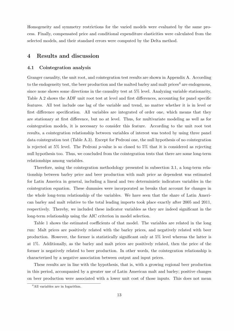
4 Results and discussion
4.1 Cointegration analysis
Granger casuality, the unit root, and cointegration test results are shown in Appendix A. According
to the endogeneity test, the beer production and the malted barley and malt prices4 are endogenous,
since none shows some directions in the causality test at 5% level. Analyzing variable stationarity,
Table A.2 shows the ADF unit root test at level and first differences, accounting for panel specific
features. All test include one lag of the variable and trend, no matter whether it is in level or
first difference specification. All variables are integrated of order one, which means that they
are stationary at first difference, but no at level. Thus, for multivariate modeling as well as for
cointegration models, it is necessary to consider this feature. According to the unit root test
results, a cointegration relationship between variables of interest was tested by using three panel
data cointegration test (Table A.3). Except for Pedroni one, the null hypothesis of no cointegration
is rejected at 5% level. The Pedroni p-value is so closed to 5% that it is considered as rejecting
null hypothesis too. Thus, we concluded from the cointegration tests that there are some long-term
relationships among variables.
Therefore, using the cointegration methodology presented in subsection 3.1, a long-term rela-
tionship between barley price and beer production with malt price as dependent was estimated
for Latin America in general, including a lineal and two deterministic indicators variables in the
cointegration equation. These dummies were incorporated as breaks that account for changes in
the whole long-term relationship of the variables. We have seen that the share of Latin Ameri-
can barley and malt relative to the total leading imports took place exactly after 2005 and 2011,
respectively. Thereby, we included these indicator variables as they are indeed significant in the
long-term relationship using the AIC criterion in model selection.
Table 1 shows the estimated coefficients of that model. The variables are related in the long
run: Malt prices are positively related with the barley prices, and negatively related with beer
production. However, the former is statistically significant only at 5% level whereas the latter is
at 1%. Additionally, as the barley and malt prices are positively related, then the price of the
former is negatively related to beer production. In other words, the cointegration relationship is
characterized by a negative association between output and input prices.
These results are in line with the hypothesis, that is, with a growing regional beer production
in this period, accompanied by a greater use of Latin American malt and barley; positive changes
on beer production were associated with a lower unit cost of those inputs. This does not mean
4All variables are in logarithm.
13

Table 1: Parameter estimates for cointegration equation of malt price on barley price and beer
production in Latin America
Variable Coefficients
ln(Barley price) 0.011**
ln(Beer production) -0.428***
linear 0.924***
After 2005 -0.027***
After 2011 2.187***
Constant 0.012
R2 0.860
Adj −R2 0.783
RMSE 0.172
Note: *** statistically significant at 1% level, ** significant at 5% level
that the input prices had a decreasing trend along the period (in fact, it is increasing as shown in
Figure 3) while the production increased. Actually, a long-term stable relationship between these
variables was confirmed and kept even when the increases in production levels resulted in decreases
in the input prices, and vice versa. Specifically, Table 1 shows that when beer production increased
by 1 percent, malt prices felt by 0.43% on average over the whole period in the Latin American
region.
Since the endogeneity of the three variables was statistically confirmed by causality tests, an-
other interpretation of these results could be that beer production responds positively to cheaper
inputs, which is expected from the microeconomic theory.
Figure 3: Evolution of input prices by origin
(a) Barley prices (b) Malt prices
Source: Own elaboration.
Although we identified a growing beer production in this period with a greater use of Latin
American inputs, the cointegration results do not indicate that these input prices are lower than
14

those from other regions. In fact, as shown in Figure 3, Latin American barley prices are generally
below those of non-Latin America ones, and the opposite occurs in malt prices. Therefore, this leads
to the counterfactual question of whether this negative relationship between production and input
prices would be kept even without the appearance of Latin American barley and malt production.
This question cannot be answered with this methodology and level of data, so it represent an
extension for future research.
For the specific case of Argentina, Gianello and Vicentin Masaro (2014) found a positive long-
term relationship between the export prices of barley and beer. These results would not be consis-
tent with our results for in whole Latin America, given that there was an increasing in price and
beer production in the period. This may be due to the fact that Gianello and Vicentin Masaro
(2014) captured the price transmission from exports to the agricultural sector, while we modeled
the countries that are self-sufficient and export barley together with those that have import it
mostly for beer production.
4.2 Demand analysis for imported malt and malted barley
Pooled model estimations
The different specification log-likelihoods without homogeneity and symmetry restrictions and the
respective LR tests are presented in Table B.1. Results show that only the Rotterdam model
is not rejected by the general system, which implies a better fit to data according to the other
models. Given the model selection test results, Table B.2 shows the likelihood ratio statistics for
the constraints of homogeneity and symmetry for Rotterdam model. Whereas homogeneity is not
rejected, the hypothesis of homogeneity and symmetry is indeed rejected at 1% level. Although the
symmetry condition for the pooled model is not fulfilled, it is imposed in the estimation to make
the model consistent with economic theory.
Parameters estimated by the pooled Rotterdam model and each commodity mean shares are
presented in Table 2. Single equations R2 are 0.29, 0.22, and 0.72 for LA malt, LA barley, and
ROW malt, respectively. However, the overall determination coefficient is 0.90, which implies
that the whole system explains 90% of the variation in allocation5. The expenditure coefficient
θi shows the additional amount spent on commodity i when total imports increase by 1 dollar.
Except for barley imported from the rest of the world, all expenditure coefficients are significantly
different from zero. These coefficient magnitude implies similar preferences for malt and barley
imported from Latin America and for malt imported from non-Latin American origins to fulfill
beer production requirements. However, in general terms, the value of the expenditure coefficients
supports the fact that for the analyzed period, imports from Latin America have a greater response
5Overall R2 is computed as
1 − det(Ψ)
det(Σ),
where Ψ is the estimated covariance matrix of error terms and Σ is the estimated covariance matrix of all variables.
15

to increases in the total value of imports of inputs in the region. All own-price elasticities are
negative and statistically significant at the 5% level, with the exception of Latin American barley.
Cross price parameters reveal substitution between malt from Latin American and ROW sources
and substitution between malt and barley imports from non-Latin American countries.
Table 2: Parameter estimates for pooled Rotterdam demand model
Mean Expenditure Price coefficients: πij
share: si coefficient: θi LA malt LA barley ROW malt ROW barley
LA malt 0.38 0.310*** -0.125** 0.003 0.125** -0.003
(0.111) (0.056) (0.013) (0.050) (0.034)
LA barley 0.25 0.336* -0.113 0.059 0.051
(0.186) (0.089) (0.043) (0.043)
ROW malt 0.18 0.270*** -0.284*** 0.100**
(0.064) (0.041) (0.041)
ROW barley 0.19 0.084 -0.149***
(0.103) (0.049)
Notes: *** statistically significant at 1% level, ** significant at 5% level * significant at 10% level.
Clustered standard errors in parentheses.
Table 3 shows the import demand elasticities derived from the pooled Rotterdam model with
their respective asymptotic standard errors. Except for Latin American barley, all own-price elas-
ticities are negative and statistically significant at the 5% level. The estimated elasticities indicate
that the demand for malt from Latin America and barley from the ROW sources are price inelastic,
whereas the demand for malt from the ROW are price elastic. In fact, in absolute value, the own-
price elasticity of Latin American malt is the lowest, which would indicate a better competitive
position of the same product with respect to inputs from the rest of the world. Specifically, an
increase of 10% in the price of Latin American malt would reduce on average 3.33% the quantity
demanded by the Latin American countries considered in the pool, whereas if the price of malt
from the ROW increases in that proportion, the quantity demanded would be reduced by 15.36%
on average. In turn, barley from Latin America is totally price insensitive in statistical terms, and
this also reflects a competitive advantage for Latin American barley exporters.
Cross price elasticities indicate that malt imports from Latin America are less sensitive to
changes in price of ROW malt compared to the response of malt imports from the ROW to price
changes in Latin American malt. The values indicate that a reduction by 10% in the price of malt
imported from the ROW implies a reduction of 3.31% in the quantity of malt demanded from Latin
America. On the other hand, a 10% reduction of the price of Latin American malt is associated
with a 6.74% lower quantity of malt demanded from the ROW. This suggests that Latin America
is more price competitive than the ROW in the Latin American malt import market. Additionally,
16

we found a significant substitution between malt and barley from the ROW. On average, a 10%
increase in the price of ROW malt (ROW Barley) would increase the quantity of ROW barley
(ROW malt) demanded by Latin American countries by approximately 5%.
Finally, all expenditure elasticities are positive and statistically significant, except for ROW
barley. Latin American barley and ROW malt elasticities are greater than one, implying that on
average additional expenditure favors imports of these commodities. These elasticities provide a
characterization of how a higher outlay on imported inputs/ingredients is distributed as the result
of an increase in beer production. That is, higher expenditure on imports for beer production
generates a more than proportional increase in the demand for malt from ROW and for Latin
American barley, whereas the demand for Latin American malt grows less than proportionally. On
the one hand, this can be explained by the fact that during the period, Latin American malt is
the one with the highest average share of the total imported inputs, therefore its increase would
be smaller in proportional terms. On the other hand, these results also show that there is a trend
to spend more on imported barley for the country’s own malt production for subsequent beer
production. A greater expenditure elasticity of ROW malt could be related to issues of the quality
of certain malts for the production of specific types or brands of beer, which classifies economically
this input not as a necessity but as a luxury good for Latin American beer producers.
Table 3: Elasticity estimates for pooled Rotterdam model
Expenditure Own and cross price elasticities
elasticity LA malt LA barley ROW malt ROW barley
LA malt 0.824*** -0.332** 0.009 0.331** -0.007
(0.295) (0.149) (0.036) (0.134) (0.090)
LA barley 1.350* 0.013 -0.455 0.237 0.205
(0.748) (0.054) (0.358) (0.174) (0.174)
ROW malt 1.462*** 0.674** 0.319 -1.536*** 0.543**
(0.347) (0.273) (0.235) (0.223) (0.224)
ROW barley 0.442 -0.014 0.269 0.527** -0.782***
(0.540) (0.178) (0.228) (0.218) (0.259)
Notes: *** statistically significant at 1% level, ** significant at 5% level * significant at 10% level
Asymptotic standard errors in parentheses.
Brazil and Mexico input demand elasticities
In this subsection, we present the demand estimations for imported inputs for the two main beer-
producing countries in Latin America, that is Mexico and Brazil. We perform a separate analysis
for them, according to their relevance and particularity as malt and barley demanding countries.
Likelihood ratio tests for model selection indicate that Rotterdam and AIDS models show a
17

better fit to data for Brazil and Mexico, respectively, than the other specifications (Table B.3 in
Appendix B). In addition, homogeneity and symmetry constraints are not rejected for these two
models at 1% significance level (Table B.4 in Appendix B). Therefore, we choose the Rotterdam
specification for Brazil and the AIDS specification for Mexico to model the import behavior.
Table 4 shows parameter estimates for the Brazilian demand model and average shares of each
commodity. The overall coefficient of determination is 0.88, which implies that the variability in
allocation between these commodities is 88% explained by the whole system. For the period 2010-
2020, malt and barley comes mainly from Latin American sources, which accounts for 87% of the
total imports on average. All expenditure coefficients are positive and significantly different from
zero. Own-price coefficients are negative, but the ROW equation is statistically significant only
for malt. On the other hand, cross-price coefficients shows that both barley and malt from Latin
America compete with malt from the ROW in the Brazilian market.
Table 4: Parameter estimates for the Brazilian Rotterdam demand model
Mean Expenditure Price coefficients: πij
share: si Coefficient: θi LA malt ROW malt LA barley
LA malt 0.65 0.639*** -0.139 0.299*** -0.161
(0.045) (0.162) (0.077) (0.149)
ROW malt 0.13 0.112*** -0.490*** 0.191***
(0.026) (0.075) (0.068)
LA barley 0.22 0.249*** -0.031
(0.042) (0.157)
Notes: ***statistically significant at 1% level, ** significant at 5% level *significant at 10% level.
Robust standard errors in parentheses.
Brazilian import demand elasticities are reported in Table 5. From the own-price elasticities, we
could infer that the Brazilian demands for imported malt and malted barley from Latin America
are inelastic and not statistically different to zero. These results are consistent with the ones of the
pooled model, in the sense that the demand response for Latin American inputs is invariant under
own-price variations, which indicates an advantageous position for its exporters. On the contrary,
the Brazilian demand for malt imported from the ROW is very elastic. Specifically, a change of
10% in the price of malt from the ROW countries produces an opposite change in the quantity
demanded of 37.1% as response. Additionally, this demand is elastic with respect to Latin American
input prices (cross-price elasticities). However, demands for Latin American malt and barley are
inelastic with respect to the prices of foreign malt. Despite this, these cross-price elasticities show
that the demand for Latin American inputs would only be sensitive to the prices of malt from its
competitors from the ROW. As in the pooled case, we found that Latin American inputs are more
difficult to substitute (due to price changes) than those from the ROW; in the case of Brazil, the
18
gap between substitution possibilities is much greater.
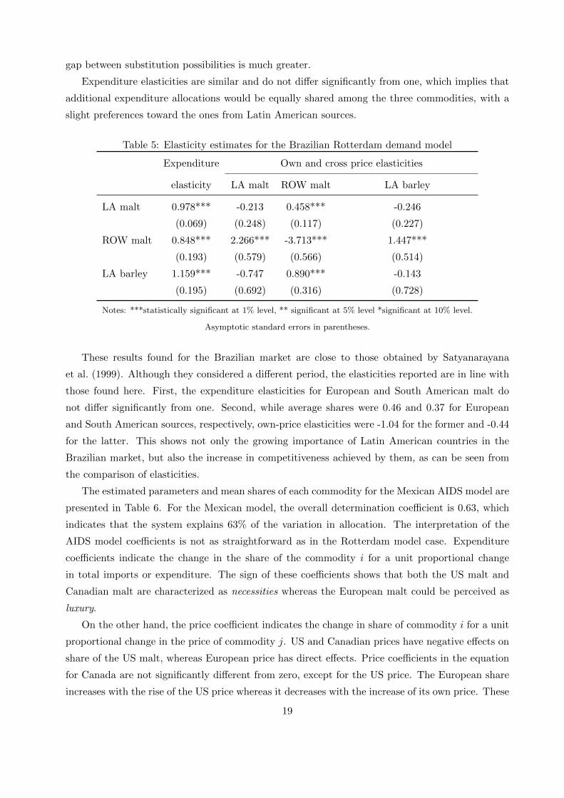
Expenditure elasticities are similar and do not differ significantly from one, which implies that
additional expenditure allocations would be equally shared among the three commodities, with a
slight preferences toward the ones from Latin American sources.
Table 5: Elasticity estimates for the Brazilian Rotterdam demand model
Expenditure Own and cross price elasticities
elasticity LA malt ROW malt LA barley
LA malt 0.978*** -0.213 0.458*** -0.246
(0.069) (0.248) (0.117) (0.227)
ROW malt 0.848*** 2.266*** -3.713*** 1.447***
(0.193) (0.579) (0.566) (0.514)
LA barley 1.159*** -0.747 0.890*** -0.143
(0.195) (0.692) (0.316) (0.728)
Notes: ***statistically significant at 1% level, ** significant at 5% level *significant at 10% level.
Asymptotic standard errors in parentheses.
These results found for the Brazilian market are close to those obtained by Satyanarayana
et al. (1999). Although they considered a different period, the elasticities reported are in line with
those found here. First, the expenditure elasticities for European and South American malt do
not differ significantly from one. Second, while average shares were 0.46 and 0.37 for European
and South American sources, respectively, own-price elasticities were -1.04 for the former and -0.44
for the latter. This shows not only the growing importance of Latin American countries in the
Brazilian market, but also the increase in competitiveness achieved by them, as can be seen from
the comparison of elasticities.
The estimated parameters and mean shares of each commodity for the Mexican AIDS model are
presented in Table 6. For the Mexican model, the overall determination coefficient is 0.63, which
indicates that the system explains 63% of the variation in allocation. The interpretation of the
AIDS model coefficients is not as straightforward as in the Rotterdam model case. Expenditure
coefficients indicate the change in the share of the commodity i for a unit proportional change
in total imports or expenditure. The sign of these coefficients shows that both the US malt and
Canadian malt are characterized as necessities whereas the European malt could be perceived as
luxury.
On the other hand, the price coefficient indicates the change in share of commodity i for a unit
proportional change in the price of commodity j. US and Canadian prices have negative effects on
share of the US malt, whereas European price has direct effects. Price coefficients in the equation
for Canada are not significantly different from zero, except for the US price. The European share
increases with the rise of the US price whereas it decreases with the increase of its own price. These
19

relationships become clearer when analyzing the elasticity estimates.
Table 6: Parameter estimates for the Mexican AIDS model
Mean Expenditure Price coefficients: γij
share: si coefficient: βi US malt Canada malt EUR malt
US malt 0.75 -0.286*** -0.163* -0.118*** 0.282***
(0.072) (0.094) (0.039) (0.102)
Canada malt 0.17 -0.088*** 0.040 0.078
(0.028) (0.036) (0.051)
EUR malt 0.08 0.374*** -0.360***
(0.076) (0.125)
Notes: *** statistically significant at 1% level, ** significant at 5% level, * significant at 10% level.
Robust standard errors in parentheses.
Table 7 shows the estimated demand elasticities for the Mexican market. Note in own-price
elasticities that the Mexican demand for malt from the US and Canada is inelastic with respect
to their own prices: on average, a 10% increase in malt prices implies a 4.6% and 5.9% reduction
in the quantities demanded, respectively. Nevertheless, the European malt import demand is very
elastic, showing that a 10% increase in its price reduces by half the quantity demanded. In addition,
in the values of cross-price elasticities, there is a high substitution in the demand for European
malt when the prices of its competitors (Canada and US) change. In turn, there are no cross-price
effects between US and Canada. Finally, as it was deduced from demand coefficients, expenditure
elasticities indicate that a higher expenditure on malt imports produces a greater proportional
weight on the demand for European malt, which is expected given its low market share in relation
to US and Canada.
When comparing with Brazil, we found similarities in the malt demand behavior of Mexico
with respect to the price of its North American neighbors and with Latin American exporters. At
the same time, in the same way that Brazil has a very elastic demand for malt imported from
the ROW (in which Belgium is the main exporter), Mexico has a very elastic demand for malt of
European origin. This would suggest a greater competitiveness (through prices) of the malt from
American countries compared to the malt from European ones. The main difference between the
demands from Mexico and Brazil is that the Latin American input demand elasticity converges to
zero whereas the US and Canada input demand is is greater than zero even when it is inelastic.
This shows a greater market positioning of Latin American countries in the Brazilian beer input
(i.e. malt and malted barley) markets than the one that North American countries have in the
Mexican malt market.
Finally, these results found for both countries reflect the role of multilateral free trade agree-
ments, that is, NAFTA for Mexico and Mercosur for Brazil, as pointed out by Mena et al. (2016)
20

in terms of the consolidation of national companies. Each one has competitive advantages in terms
of input availability from the main producer countries from the American continent: Canada and
US for Mexico, and Argentina and Uruguay for Brazil. At the same time, these malt and bar-
ley exporters have a strong competitive position reflected in high market shares, low own-price
elasticities, and high cross-price elasticities with respect to other competitors.
Table 7: Elasticity Estimates for the Mexican AIDS model
Expenditure Own and cross price elasticities
elasticity US malt Canada malt Europe malt
US malt 0.6206*** -0.4624*** 0.0144 0.4480***
(0.0954) (0.1245) (0.0519) (0.1347)
Canada malt 0.4881*** 0.0635 -0.5936*** 0.5301*
(0.1636) (0.2284) (0.2111) (0.2968)
Europe malt 6.0237*** 4.5401*** 1.2209* -5.7610***
(1.0262) (1.3656) (0.6835) (1.6800)
Notes: *** statistically significant at 1% level, ** significant at 5% level * significant at 10% level.
Asymptotic standard errors in parentheses.
5 Conclusions
In the present paper, we addressed the phenomenon of the growing demand for Latin American
malt and barley within the same region. We interpreted this phenomenon as a process of vertical
integration of the region, and from this hypothesis, the general aim of this research was to char-
acterize the phenomenon in terms of its effects on the brewing industry competitiveness as well as
on the main beer input producers/exporters. In particular, we studied the relationship between
input prices and beer production and then analyzed the behavior of Latin American countries as
importers of malt and barley from both the same and other regions, such as Europe and North
America (excluding Mexico).
This greater participation of Latin American input exporters accompanied a continuous growth
on beer production into a greater trade liberalization context, a multilateral trade agreement sign-
ing, a growing firm internationalization and more concentrated markets from numerous mergers
and acquisitions that took place in most nations in the region.
To carry out this study, we used different techniques and econometric models. First, we used
panel data cointegration techniques to quantify the long-term relationship between input prices
and beer production. Second, we estimated import demand systems to obtain imported malt and
barley demand elasticities. We used last methodology for grouped data, to model the main Latin
American countries that demand malt and barley in the region, as well as study in a disaggregated
21

way Brazil and Mexico, the two main producers in the region.
From the cointegration approach, we found a negative long-term relationship between input
prices and beer production. Therefore, we can conclude that this period with growing beer pro-
duction, characterized with a vertical integration process within the region, is consistent with the
achievement of lower input prices.
Based on the malt and malted barley import demand elasticities, a strong competitive po-
sitioning of Latin American exporters is observed, supported by increasing shares in importing
markets, lower (and in some cases, zero) own-price elasticities, and lower sensitivity with respect to
the competing prices from countries in other regions. On the other hand, expenditure elasticities
allow Latin American inputs to be classified in microeconomic terms as necessary goods for beer
production, whereas those from the rest of the world are classified as luxury goods.
Finally, it is clear the role that free trade agreements play on the main beer producers of
the region, that is, Mexico and Brazil, which based on NAFTA and Mercosur, achieved a bloc
integration with a strong competitive positioning of malt and barley exporters.
References
Alfaro, L., Conconi, P., Fadinger, H., and Newman, A. F. (2016). “Do Prices Determine Vertical
Integration?” Review of Economic Studies, 83 (3), 855–888.
Barten, A. P. (1964). “Consumer demand functions under conditions of almost additive prefer-
ences.” Econometrica: Journal of the Econometric Society, 1–38.
Barten, A. P. (1993). “Consumer allocation models: choice of functional form.” Empirical Eco-
nomics, 18 (1), 129–158.
Benıtez, L., and Torda, A. (2019). “Evaluating the performance of merger simulation using different
demand systems: Evidence from the Argentinian beer market.”
Berlingieri, G., Pisch, F., and Steinwender, C. (2018). “Organizing Global Supply Chains: In-
put Cost Shares and Vertical Integration.” NBER Working Papers 25286, National Bureau of
Economic Research, Inc.
Blecher, E., Liber, A., Van Walbeek, C., and Rossouw, L. (2018). “An international analysis of the
price and affordability of beer.” PLOS ONE, 13 (12), 1–16.
Brown, M., Lee, J.-Y., and Seale Jr, J. (1994). “Demand relationships among juice beverages:
A differential demand system approach.” Journal of Agricultural and Applied Economics, 26,
417–429.
Bullard, A. (2004). “Competition policies, market competitiveness and business efficiency: lessons
22

from the beer sector in Latin America.” In U. Nations (Ed.), Competition, Competitiveness and
Development: Lessons from Developing Countries, 143–169, New York: United Nations.
Casarin, A. A., Cornejo, M., and Delfino, M. E. (2019). “Market power absent merger review:
Brewing in Peru.” Review of Industrial Organization, 1–22.
Choi, I. (2001). “Unit root tests for panel data.” Journal of International Money and Finance,
20 (2), 249–272.
Colino, E., Civitaresi, H. M., Capuano, A., Quiroga, J. M., and Winkelman, B. (2017). “Analisis
de la estructura y dinamica del complejo cervecero artesanal de Bariloche, Argentina.” Revista
Pilquen-Seccion Ciencias Sociales, 20 (2), 79–91.
de Freitas, A. G. (2015). “Relevancia do mercado cervejeiro brasileiro: avaliacao e perspectivas e a
busca de uma agenda de regulacao.” Pensamento & Realidade, 30 (2).
de Oliveira Dias, M., and Falconi, D. (2018). “The evolution of craft beer industry in Brazil.”
Journal of Economics and Business, 1 (4), 618–626.
Deaton, A., and Muellbauer, J. (1980). “An almost ideal demand system.” The American economic
review, 70 (3), 312–326.
Duarte Alonso, A., Kok, S., and O’Shea, M. (2020). “Peru’s emerging craft-brewing industry and
its implications for tourism.” International Journal of Tourism Research.
Eales, J. S., and Unnevehr, L. J. (1988). “Demand for beef and chicken products: separability and
structural change.” American Journal of Agricultural Economics, 70 (3), 521–532.
Eales, J. S., and Unnevehr, L. J. (1993). “Simultaneity and structural change in US meat demand.”
American Journal of Agricultural Economics, 75 (2), 259–268.
Erdil, E. (2006). “Demand systems for agricultural products in OECD countries.” Applied Eco-
nomics Letters, 13, 163–169.
Gianello, L., and Vicentin Masaro, J. (2014). “Transmision entre precios de exportacion: cebada
cervecera y cerveza.” In A. A. de Economıa Agraria (Ed.), Anales de la XLV Reunion Anual
2014 y IV Congreso Regional.
Hart, O., and Tirole, J. (1990). “Vertical integration and market foreclosure.” Brookings Papers on
Economic Activity, 21 (1990 Microeconomics), 205–286.
Kao, C. (1999). “Spurious regression and residual-based tests for cointegration in panel data.”
Journal of Econometrics, 90 (1), 1–44.
Keller, W. J., and Van Driel, J. (1985). “Differential consumer demand systems.” European Eco-
nomic Review, 27 (3), 375–390.
23

Khodzhimatov, R. (2018). “XTCOINTREG: Stata module for panel data generalization of coin-
tegration regression using fully modified ordinary least squares, dynamic ordinary least squares,
and canonical correlation regression met.” Statistical Software Components, Boston College De-
partment of Economics.
Laitinen, K. (1980). “A theory of the multiproduct firm.” In H. Theil, and H. Glejser (Eds.), Studies
in Mathematical and Managerial Economics, chap. 28, New York: North Holland.
Laitinen, K., and Theil, H. (1978). “Supply and demand of the multiproduct firm.” European
Economic Review, 11 (2), 107 – 154.
Lee, J.-Y., Brown, M. G., and Seale Jr, J. L. (1994). “Model choice in consumer analysis: Taiwan,
1970–89.” American Journal of Agricultural Economics, 76 (3), 504–512.
McAfee, R. P. (1999). “The effects of vertical integration on competing input suppliers.” Economic
Review, (Q I), 2–8.
Mena, L. A. R., Vidales, K. B. V., and Garcıa, J. O. G. (2016). “South of the border: The beer and
brewing industry in South America.” In I. Cabras, D. Higgins, and D. Preece (Eds.), Brewing,
Beer and Pubs: A Global Perspective, 162–181, London: Palgrave Macmillan UK.
MinAgri (2016). “Informe de cebada.”
Neves, P. (1987). “Analysis of consumer demand in Portugal, 1958-198.” Tech. rep., Louvain-la-
Neuve.
Ordover, J. A., Saloner, G., and Salop, S. C. (1990). “Equilibrium vertical foreclosure.” The Amer-
ican Economic Review, 80 (1), 127–142.
Pedroni, P. (1999). “Critical values for cointegration tests in heterogeneous panels with multiple
regressors.” Oxford Bulletin of Economics and statistics, 61 (S1), 653–670.
Rendon, L., and Mejia, P. (2005).
Salinger, M. A. (1988). “Vertical mergers and market foreclosure.” The Quarterly Journal of Eco-
nomics, 103 (2), 345–356.
Satyanarayana, V., Wilson, W. W., and Johnson, D. D. (1999). “Import demand for malt in selected
countries: A linear approximation of AIDS.” Canadian Journal of Agricultural Economics/Revue
canadienne d’agroeconomie, 47 (2), 137–149.
Swinnen, J. (Ed.) (2011). The Economics of Beer. Oxford University Press.
Swinnen, J., and Briski, D. (2017). Beeronomics: How Beer Explains the World. No. 9780198808305
in OUP Catalogue, Oxford University Press.
24

Theil, H. (1965). “The analysis of disturbances in regression analysis.” Journal of the American
Statistical Association, 60 (312), 1067–1079.
Thome, K., and Soares, A. (2015). “International market structure and competitiveness at the
malted beer: from 2003 to 2012.” Agricultural Economics – Czech, 61, 166–178.
Toro-Gonzalez, D. (2015). “The Beer Industry in Latin America.” AAWE Working Paper 177,
American Association of Wine Economists.
Toro-Gonzalez, D. (2017). “The Craft Brewing Industry in Latin America.” Choices: The Magazine
of Food, Farm, and Resource Issues, 32 (3).
Toro-Gonzalez, D. (2018). “The craft brewing industry in Latin America: The case of Colombia.”
In Economic Perspectives on Craft Beer, 115–136, Springer.
Trujillo-Sandoval, D., Puente-Guijarro, C., and Andrade-Quevedo, K. (2018). “Concentracion
economica en el mercado cervecero ecuatoriano.” Ciencia Unemi, 10 (25), 67–78.
Wang, Q., and Wu, N. (2012). “Long-run covariance and its applications in cointegration regres-
sion.” The Stata Journal, 12 (3), 515–542.
Washington, A. A., and Kilmer, R. L. (2002). “The production theory approach to import demand
analysis: A comparison of the Rotterdam model and the differential production approach.”
Journal of Agricultural and Applied Economics, 34 (3), 431–443.
Westerlund, J. (2005). “New simple tests for panel cointegration.” Econometric Reviews, 24 (3),
297–316.
WHO (2018). “Global status report on alcohol and health 2018. World Health Organization.”
WTEx (2020). “World’s top exports: Beer exports by country.” url:
http://www.worldstopexports.com/beer-exports-by-country/, accessed: 2020-10-08.
Yenne, B. (2014). Beer: The ultimate world tour. Race Point Pub.
25

Appendices
A Tests for cointegration analysis
Table A.1: Granger-causality test
H0 z-bar estadistic p-value
Beer production does not cause Barley price 2.217 0.027
Beer production does not cause Malt price 8.038 0.000
Barley price does not cause Beer production 8.979 0.000
Barley price does not cause Malt price 5.796 0.000
Malt price does not cause Beer production 3.049 0.002
Malt price does not cause Barley price 8.038 0.000
Notes: Granger – causality test, accounting panel data features
Table A.2: Augmented Dickey Fuller unit root tests
Variables Level First difference
Beer production1.98 -13.13
[0.976] [0.000]
Barley price0.054 -7.44
[0.522] [0.000]
Malt price1.001 -5.504
[0.842] [0.000]
# Panels 17
Notes: data in brackets are p-values
Table A.3: Cointegration tests
Statistic p-value
Kao* 2.5103 0.006
Pedroni* 1.5757 0.0575
Westerlund** -2.2191 0.0132
# Panles 17
Notes* are ADF statistics, ** are variance ratio
B Tests for demand analysis
26

Table B.1: Test results for model selection
Log likelihoodsa LRb
General 640.9608
Rotterdam 638.4166 5.0884
AIDS 623.8189 34.2836
CBS 628.5854 24.7508
NBR 632.2119 17.4977
a Log likelihoods from unrestricted models, that is,
without homogeneity and symmetry.
b Table value for χ22 at α = 0.01 is 9.21.
Table B.2: Test results for Rotterdam model constraints
Log likelihoods LRa
Unrestricted 638.4166
Homogeneity 634.3502 8.1327(3)
Homogeneity and symmetry 624.4001 28.0330(6)
a Degrees of freedom in parentheses.
Table values for χ23 and χ2
6 at α = 0.01 are 11.34 and 16.81, respectively.
Table B.3: Test results for model selection
Brazil Mexico
Log likelihoodsa LRb Log likelihoodsa LRb
General model 1206.6641 1299.4450
Rotterdam 1205.5415 2.2452 1292.8442 13.2016
AIDS 1202.5699 8.1884 1298.9575 0.9750
CBS 1203.7450 5.8382 1297.5022 3.8856
NBR 1205.1728 2.9826 1294.0875 10.7150
a Log likelihoods from unrestricted models, that is, without homogeneity and symmetry.
b Table value for χ22 at α = 0.01 is 9.21.
27

Table B.4: Test results for model constraints
Brazil Rotterdam Mexico AIDS
Log likelihoods LRa Log likelihoods LRa
Unrestricted 1205.5415 1298.9575
Homogeneity 1204.3056 2.4718(2) 1295.1225 7.6700(2)
Homogeneity and symmetry 1202.7631 5.5568(3) 1294.4805 8.9540(3)
a Degrees of freedom in parentheses. Table values for χ22 and χ2
3 at α = 0.01 are 9.21 and 11.34, respectively.
28