laszl´ o m´ arkus´ department of probability th

Tail estimation for nonlinear stationary models

Laszlo MarkusDepartment of Probability Th. & Statistics,

Eotvos Lorand University

April 27, 2015

Laszlo Markus, Eotvos Lorand University Tail estimation for nonlinear stationary models April 27, 2015 1 / 57

Introduction

Occurrence of extremes

Tails of distributions control the occurrence of unusually large or lowvalues in the sample, i.e. the occurrence of extremal events.Extreme values are important in environmental modelling, industrialsafety planning and assessment, reserves calculations in insurances,valuation of risky financial assets and credit portfolios, and the row canbe continued.So, there is no doubt about the practical use of inference on the tailestimations.


Introduction

The influence of the dynamics

When the phenomenon in question is time dependent and generated bya dynamics from a random source the nature of the dynamics cansignificantly influence the occurrence of the extremes.By and large, linear systems respond to a driving force by an output ofapproximately the same nature, whereas when nonlinearity is presenteven bounded induction can trigger an unbounded response. So it is ofutmost importance to understand the nature of nonlinearities and takeinto account their presence when modelling.In the introductory talk I’m going to give a survey of classical results fortail behaviour of time series of various linear and non-linear dynamics.


Introduction

Tails of the stationary distributions

We wish to concentrate mainly on the strictly stationary time series drivenby the considered dynamics. To this end we suppose that there exists astrictly stationary process generated by the dynamics from an i.i.d. noisein a causal way (current values are independent of the future of thenoise). The distribution of such a process is unique given the noisedistribution.For the stationary series the marginal distribution is the same for everyX (t), and it is the tail of this marginal distribution that we are interested in.

driving noise (i.i.d.)dynamics

=⇒ structured process.

noise distributiondynamics

=⇒ stationary distribution.It is not straightforward to determine the stationary distribution.


Introduction

First order autoregression, causal solution

Let ε(t) be an independent value noise i.e. an i.i.d. sequence. Mostly, butnot necessarily Eε(t) = 0.First order autoregression:

X (t) = αX (t−1) + σε · ε(t). (1)

Iterating the equation, elementary considerations yield that a causalstationary solution exists if and only if |α|< 1.In terms of the noise this causal stationary solution can be written as

X (t) =∞

∑u=0

αu · ε(t−u)

and the sum is convergent both in L2 and almost surely.In particular we see here that the causal AR(1) process has arepresentation as the linear combination of the past values of the noise,hence it is a causal linear process.


Introduction

Stationary distributions of AR(1) models, normal noise

For the causal solution X (t−1) and ε(t) are independent, and whenε(t)-s are N(0,1) distributed, then the stationary solution has normalmarginals, X (t) = N(0,σ2

X ) with σ2X = σ2

ε

1−α2

This assertion relies heavily on the fact that the normal family is closedunder summation.Is it also that easy to get the stationary distribution of such a simplemodel for different noises?


Introduction

Stationary distributions of AR(1) models, discretenoise

Suppose ε(t) takes only two values 0 and 12 , and

P(ε(t) = 1

2

)= P (ε(t) = 0) = 1

2 .

With the autoregressive parameter α = 12 the stationary solution of the

equation X (t) = 12X (t−1) + ε(t) can be written as

∞

∑u=0

(12

)u

ε(t−u) =∞

∑u=0

(12

)u+1

·2ε(t−u).

2ε(t−u) is a random 0-1 sequence. Multiplied by the powers of 12 any

real number in [0,1] can be obtained in the limit, and as every 0-1sequence ”uniformly probable”, the distribution of the produced numberswill be uniform on [0,1]. So the a stationary distribution will be U(0,1).As we’ve seen discrete noise may generate absolutely continuousstationary distribution.


Introduction

Prescribed stationary distributions of AR(1) models

We may consider the question on the other way round. Does there existan i.i.d. noise sequence that generates a prescribed distribution as thestationary one of the AR(1) model with a suitable parameter α?If the solution we are looking for is a positive random variable then α

must be taken from the (0,1) interval rather than from (-1,1). In this caseLaplace transforms may be of help.Indeed taking Laplace transform of the autoregressive equation we get

Lε (s) = LX (s)/LX (αs).

This equation opens the way to construct an AR(1) process with theprescribed stationary distribution if and only if Lε (s) is the Laplacetransform of a distribution.


Introduction

Self decomposable distributions of AR(1) models

Gaver and Lewis pointed out that Lε (s) is the Laplace transform of adistribution iff the prescribed stationary distribution is self decomposablei.e. φ(t) = φ(αt)φα (t) holds for its characteristic function φ(t) with someother characteristic function φα (t) for every α ∈ (0,1). In terms of randomvariables it means that X has to be decomposable as X = αX + Xα forevery α ∈ (0,1), with an Xα independent of X.(Equality is meant here indistribution only.)All non-degenerate self decomposable distributions are absolutelycontinuous.Self decomposable distributions are a proper class of the infinitelydivisible distributions and contain the stable, gamma, inverse Gaussian,hyperbolic distributions just as the CGMY (Carr-Geman-Madan-Yor)distribution of mathematical finance.


Introduction

An example and some references

All these self decomposable distributions, not just the positive ones, mayserve as stationary distributions of AR(1) processes, see e.g.Loeve(1945), Bunge(1997), but even they do not exhaust that class.In particular, if Xt is prescribed to have the exponential distribution ofparameter λ then the noise has to have a mixture distribution that is 0with probability α, and exponential Exp(λ ) with probability 1-α.


Introduction

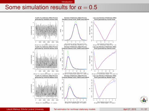
Some simulation results for α = 0.5

0 1000 2000 3000 4000 5000

−4

−2

02

4

A path of a stationary AR(1) Processgenerated by standard normal noise

timeAR par= 0.5 , Normal pars: mean=0, var= 1.33

rts1

[250

00:3

0000

]

−4 −2 0 2 4

0.0

0.1

0.2

0.3

0.4

Density of Stationary AR(1) ProcessStandard normal noise, 50000 observations

blue=empirical, red=par−fitted, green=noiseAR par= 0.5 , Normal pars: mean=0, var= 1.33

den$

y

−4 −2 0 2 4

0.0

0.5

1.0

1.5

2.0

2.5

Log−Log−Density of Stationary AR(1)series generated by normal noise

blue=empirical, red=par−fittedAR par= 0.5 , Normal pars: mean=0, var= 1.33

log(

−lo

g(de

n$y)

)

0 1000 2000 3000 4000 5000

−5

05

1015

A path of a stationary AR(1) Processgenerated by centered Gamma noise

timeAR par= 0.5 , Gamma pars, shape= 1.5 , scale= 0.5

rts1

[250

00:3

0000

]

−5 0 5 10 15 20

0.00

0.05

0.10

0.15

0.20

0.25

Density of Stationary AR(1) ProcessCentered Gamma noise, 50000 observations

blue=empirical, red=par−fitted, green=noiseAR par= 0.5 , Gamma pars, shape= 1.5 , scale= 0.5

den$

y

−5 0 5 10 15 20

0.5

1.0

1.5

2.0

2.5

Log−Log−Density of Stationary AR(1) series generated by Gamma noise

blue=empirical, red=par−fittedAR par= 0.5 , Gamma pars, shape= 1.5 , scale= 0.5

log(

−lo

g(de

n$y)

)

0 1000 2000 3000 4000 5000

−1

01

23

4

A path of a stationary AR(1) Processgenerated by centered Weibull noise

timeAR par= 0.5 , Weibull shape= 1.5 , scale=1

rts1

[250

00:3

0000

]

−2 −1 0 1 2 3 4 5

0.0

0.2

0.4

0.6

0.8

1.0

Density of Stationary AR(1) ProcessCentered Weibull noise, 50000 observations

blue=empirical, red=par−fitted, green=noiseAR par= 0.5 , Weibull shape= 1.5 , scale=1

den$

y

−2 −1 0 1 2 3 4 5

−0.

50.

51.

01.

52.

02.

5

Log−Log−Density of Stationary AR(1) series generated by Weibull noise

blue=empirical, red=par−fittedAR par= 0.5 , Weibull shape= 1.5 , scale=1

ld


Introduction

Some simulation results for α = 0.9

0 1000 2000 3000 4000 5000

−5

05

10

A path of a stationary AR(1) Processgenerated by standard normal noise

timeAR par= 0.9 , Normal pars: mean=0, var= 5.26

rts1

[250

00:3

0000

]

−10 −5 0 5 10

0.0

0.1

0.2

0.3

0.4

Density of Stationary AR(1) ProcessStandard normal noise, 50000 observations

blue=empirical, red=par−fitted, green=noiseAR par= 0.9 , Normal pars: mean=0, var= 5.26

den$

y

−10 −5 0 5 10

0.5

1.0

1.5

2.0

2.5

Log−Log−Density of Stationary AR(1)series generated by normal noise

blue=empirical, red=par−fittedAR par= 0.9 , Normal pars: mean=0, var= 5.26

log(

−lo

g(de

n$y)

)

0 1000 2000 3000 4000 5000

−10

010

2030

A path of a stationary AR(1) Processgenerated by centered Gamma noise

timeAR par= 0.9 , Gamma pars, shape= 1.5 , scale= 0.5

rts1

[250

00:3

0000

]

−20 −10 0 10 20 30 40

0.00

0.05

0.10

0.15

0.20

0.25

Density of Stationary AR(1) ProcessCentered Gamma noise, 50000 observations

blue=empirical, red=par−fitted, green=noiseAR par= 0.9 , Gamma pars, shape= 1.5 , scale= 0.5

den$

y

−20 −10 0 10 20 30 40

1.0

1.5

2.0

2.5

Log−Log−Density of Stationary AR(1) series generated by Gamma noise

blue=empirical, red=par−fittedAR par= 0.9 , Gamma pars, shape= 1.5 , scale= 0.5

log(

−lo

g(de

n$y)

)

0 1000 2000 3000 4000 5000

−4

−2

02

4

A path of a stationary AR(1) Processgenerated by centered Weibull noise

timeAR par= 0.9 , Weibull shape= 1.5 , scale=1

rts1

[250

00:3

0000

]

−4 −2 0 2 4 6 8

0.0

0.2

0.4

0.6

0.8

1.0

Density of Stationary AR(1) ProcessCentered Weibull noise, 50000 observations

blue=empirical, red=par−fitted, green=noiseAR par= 0.9 , Weibull shape= 1.5 , scale=1

den$

y

−4 −2 0 2 4 6 8

0.5

1.0

1.5

2.0

2.5

Log−Log−Density of Stationary AR(1) series generated by Weibull noise

blue=empirical, red=par−fittedAR par= 0.9 , Weibull shape= 1.5 , scale=1

ld


Linear Models

Linear Processes

The series Xt is a causal linear process if Xt =∞

∑u=0

cuεt−u, where εu is an

independent value noise, i.e. an i.i.d. sequence. General linearprocesses have the two sided representation

Xt =∞

∑u=−∞

cuεt−u. (2)

In general they are non - causal as their value depends on the future ofthe noise. Following Rootzen we shall consider general linear processes.We suppose that at least one of cu-s is positive.

Although∞

∑u=−∞

c2u < ∞ would be enough for (2) to converge in L2 when

Eε2t < ∞, if we have only E |εt |< ∞, the stronger

∞

∑u=−∞

|cu|< ∞ ensures

convergence of the sum with probability 1 (Brockwell, Davis, p.49). Weassume this latter condition throughout the rest of the talk.


Linear Models

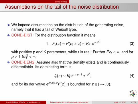
Assumptions on the tail of the noise distribution

We impose assumptions on the distribution of the generating noise,namely that it has a tail of Weibull type.COND-DIST: For the distribution function it means

1−Fε (z) = P(εt > z)∼ Kzr e−zp(3)

with positive p and K parameters, while r is real. Further Eεt < ∞, and forp > 1 Eε2

t < ∞.COND-DENS: Assume also that the density exists and is continuouslydifferentiable. Its dominating term is

fε (z)∼ Kpzr+p−1e−zp, (4)

and for its derivative econst ·z f ′(z) is bounded for z ∈ (−∞,0).


Linear Models

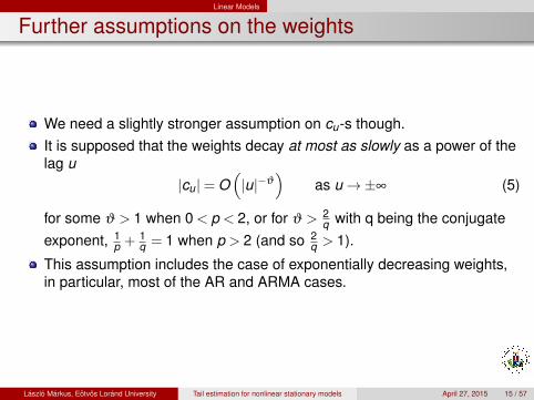
Further assumptions on the weights

We need a slightly stronger assumption on cu-s though.It is supposed that the weights decay at most as slowly as a power of thelag u

|cu|= O(|u|−ϑ

)as u→±∞ (5)

for some ϑ > 1 when 0 < p < 2, or for ϑ > 2q with q being the conjugate

exponent, 1p + 1

q = 1 when p > 2 (and so 2q > 1).

This assumption includes the case of exponentially decreasing weights,in particular, most of the AR and ARMA cases.


Linear Models

Notations related to the weights

We shall denote by ‖c‖q the usual `q norm(

∞

∑u=−∞

|cu|q < ∞

) 1q.

Further, let the constants c+,c− be:

c+ = max(cu : u = . . .−1,0,1, . . .),c− = sup(−cu : u = . . .−1,0,1, . . .),

the sup is not being attained only when all cu > 0 and then c− = 0 fromthe conditions on cu and above. Define also the sequences

c+u = max(0,cu), u = . . .−1,0,1, ...,

c−u = max(0,−cu), u = . . .−1,0,1, ...,

and the constant

γ =

(c+c−

)p

.


Linear Models

Three cases of interest, when 0 < p ≤ 1

There are three cases of interest, the case of positive weights (PW), thebalanced tails (BT), and the dominating (right) tails (DT).0 < p ≤ 1PW. The weights are non-negative: cu ≥ 0 and satisfy (5)*, furthermoreCOND-DIST holds true for the noise tail.BT. (5)* for the weights and COND-DIST for the right tail holds, while for

the left tail P(εt < z)∼ K−zr e−zp

γ as z→−∞.DT. (5)* holds for the weights, COND-DIST is imposed on the right tail,

whereas for negative z values P(εt < z) = o(

e−zp

γ

)as z→−∞.

* recall: |cu |= O(|u|−ϑ

)as u→±∞


Linear Models

The three cases of interest, when p > 1

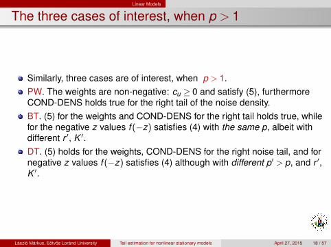
Similarly, three cases are of interest, when p > 1.PW. The weights are non-negative: cu ≥ 0 and satisfy (5), furthermoreCOND-DENS holds true for the right tail of the noise density.BT. (5) for the weights and COND-DENS for the right tail holds true, whilefor the negative z values f (−z) satisfies (4) with the same p, albeit withdifferent r ′, K ′.DT. (5) holds for the weights, COND-DENS for the right noise tail, and fornegative z values f (−z) satisfies (4) although with different p′ > p, and r ′,K ′.


Linear Models

Tails of the linear process, when 0 < p < 1

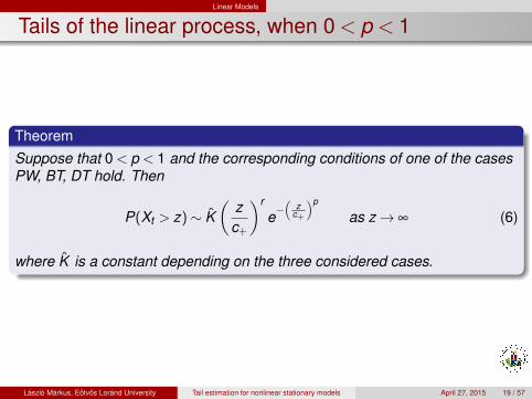
TheoremSuppose that 0 < p < 1 and the corresponding conditions of one of the casesPW, BT, DT hold. Then

P(Xt > z)∼ K(

zc+

)r

e−(

zc+

)p

as z→ ∞ (6)

where K is a constant depending on the three considered cases.


Linear Models

Tails of the linear process, when p = 1

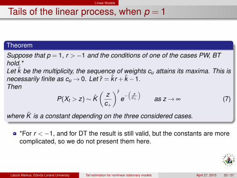
TheoremSuppose that p = 1, r >−1 and the conditions of one of the cases PW, BThold.*Let k be the multiplicity, the sequence of weights cu attains its maxima. This isnecessarily finite as cu → 0. Let r = k r + k −1.Then

P(Xt > z)∼ K(

zc+

)r

e−(

zc+

)as z→ ∞ (7)

where K is a constant depending on the three considered cases.

*For r <−1, and for DT the result is still valid, but the constants are morecomplicated, so we do not present them here.


Linear Models

Tails of the linear process, when p > 1

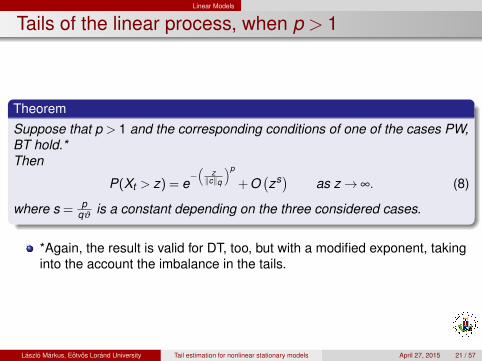
TheoremSuppose that p > 1 and the corresponding conditions of one of the cases PW,BT hold.*Then

P(Xt > z) = e−(

z‖c‖q

)p

+ O(zs) as z→ ∞. (8)

where s = pqϑ

is a constant depending on the three considered cases.

*Again, the result is valid for DT, too, but with a modified exponent, takinginto the account the imbalance in the tails.


Linear Models

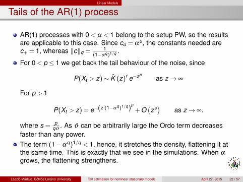
Tails of the AR(1) process

AR(1) processes with 0 < α < 1 belong to the setup PW, so the resultsare applicable to this case. Since cu = αu, the constants needed arec+ = 1, whereas ‖c‖q = 1

(1−αq)1/q .

For 0 < p ≤ 1 we get back the tail behaviour of the noise, since

P(Xt > z)∼ K (z)r e−zpas z→ ∞

For p > 1

P(Xt > z) = e−(z·(1−αq)1/q)p

+ O(zs) as z→ ∞.

where s = pqϑ

. As ϑ can be arbitrarily large the Ordo term decreasesfaster than any power.The term (1−αq)1/q < 1, hence, it stretches the density, flattening it atthe same time. This is exactly that we see in the simulations. When α

grows, the flattening strengthens.


Linear Models

Maxima of the linear process, when p > 1

Suppose that p > 1 and the corresponding conditions of one of the casesPW, BT hold. (Similar result holds true for DT as well.)Let Mn denote the sequence of the maxima Mn = max{X1, . . . ,Xn}.Then

P(an(Mn−bn ≤ x)→ e−e−xas n→ ∞. (9)

where the norming constants

an = p1‖c‖q

(logn)1p , bn = ‖c‖q(logn)

1q + O(logn)

1−ϑ

qϑ

are the same as for the associated independent sequence.In other words, the stationary distribution is in the maximum domain ofattraction of the Gumbel distribution.


Linear Models

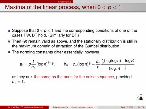
Maxima of the linear process, when 0 < p < 1

Suppose that 0 < p < 1 and the corresponding conditions of one of thecases PW, BT hold. (Similarly for DT.)Then (9) remain valid as above, and the stationary distribution is still inthe maximum domain of attraction of the Gumbel distribution.The norming constants differ essentially, however,

an = p1

c+(logn)1− 1

p , bn = c+(logn)1p +

c+p

rp (log logn) + logK

(logn)1− 1p

as they are the same as the ones for the noise sequence, providedc+ = 1.


Linear Models

On the maxima in general

In summary,the b-s that give the center of the distribution of the maxima are of theorder (logn)

1p in all cases, which tends to infinity with n.

The a-s are of the order (logn)1− 1p , which tends to infinity for p > 1, thus

showing that the scale of extremes decreases in this case, whereas ittends to zero for 0 < p < 1, corresponding to the increasing scale ofextremes, and remains constant for p=1.


Linear Models

On the maxima in general

Resnick and Davis consider the case when the distribution of the noise isentirely different, i.e. it is regularly varying at 0. They show that if we consideronly finite moving averages then the marginal distribution of the stationarylinear process will also have regular variation around 0. To the contrary,infinite moving averages under quite general conditions will not remainregularly varying at 0. In particular, ARMA processes with exponentiallydecreasing weights satisfy these conditions. When the maxima of thoseinfinite moving averages are concerned, the distribution will tend to a Weibulltype one, hence the stationary distribution belongs to the maximum domain ofattraction of the Weibull type.


Non-Linear Models

Non-Linear Processes

Though clearly, all processes that doesn’t belong to the linear class arecalled non-linear processes, the notion is still vague to some extent. Thereason is that non-linear processes does not have a canonic form, hencea unified approach is not viable, as opposed to the case of the linearprocesses. As a consequence, various model classes may be consideredseparately, and the results established within that class.Non-linear dynamics can create phenomena that linear systems arenever capable of. One such thing is e.g. the presence of attractors, orchaotic behaviour.Non-linearities make the system far more sensible to sudden changes orshocks.


Non-Linear Models

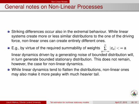
General notes on Non-Linear Processes

Striking differences occur also in the extremal behaviour. While linearsystems create more or less similar distributions to the one of the drivingforce, non-linear ones can create entirely different ones.

E.g., by virtue of the required summability of weights∞

∑u=−∞

|cu|< ∞ a

linear dynamics driven by a generating noise of bounded distribution will,in turn generate bounded stationary distribution. This does not remain,however, the case for non-linear dynamics.While linear dynamics tend to flatten the distributions, non-linear onesmay also make it more peaky with much heavier tail.


Non-Linear Models

ARCH−GARCH Processes

One of the most frequently considered model class of non-linear time series isthe (General) Autoregressive Conditionally Heteroscedastic one, theARCH−GARCH. Let ε(t) be an i.i.d. noise, with D2ε(t) = 1, whenever D2ε(t)is finite, and

X (t) = σ(t)ε(t) (10)

with the time dependent variance σ2(t), that is in the ARCH(p) casesupposed to be conditional on past values of the process, and as such to be aquadratic function of the past:

σ2(t) = α0 +

p

∑i=1

αi X 2(t− i) (11)

with positive constants αi > 0, i = 0,1, . . . ,p. The conditional variance in theGARCH(p,q) case is dependent in addition on past values of the variance, aswell:

σ2(t) = α0 +

p

∑i=1

αi X 2(t− i)+q

∑j=1

βj σ2(t− j), (12)

where αi > 0, i = 0,1, . . . ,p and βj > 0, j = 1, . . . ,q holds true, too.


Non-Linear Models

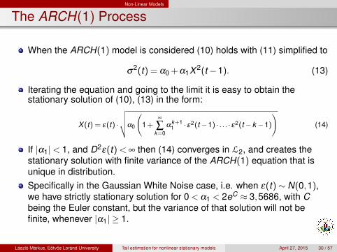
The ARCH(1) Process

When the ARCH(1) model is considered (10) holds with (11) simplified to

σ2(t) = α0 + α1X 2(t−1). (13)

Iterating the equation and going to the limit it is easy to obtain thestationary solution of (10), (13) in the form:

X(t) = ε(t) ·

√√√√α0

(1+

∞

∑k=0

αk+11 · ε2(t−1) · . . . · ε2(t−k −1)

)(14)

If |α1|< 1, and D2ε(t) < ∞ then (14) converges in L2, and creates thestationary solution with finite variance of the ARCH(1) equation that isunique in distribution.Specifically in the Gaussian White Noise case, i.e. when ε(t)∼ N(0,1),we have strictly stationary solution for 0 < α1 < 2eC ≈ 3,5686, with Cbeing the Euler constant, but the variance of that solution will not befinite, whenever |α1| ≥ 1.


Non-Linear Models

Stochastic Recurrence Equations

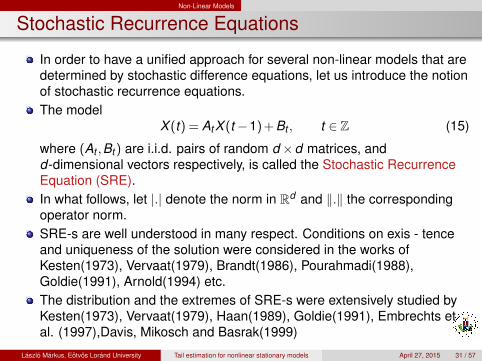
In order to have a unified approach for several non-linear models that aredetermined by stochastic difference equations, let us introduce the notionof stochastic recurrence equations.The model

X (t) = AtX (t−1) + Bt , t ∈ Z (15)

where (At ,Bt ) are i.i.d. pairs of random d ×d matrices, andd-dimensional vectors respectively, is called the Stochastic RecurrenceEquation (SRE).In what follows, let |.| denote the norm in Rd and ‖.‖ the correspondingoperator norm.SRE-s are well understood in many respect. Conditions on exis - tenceand uniqueness of the solution were considered in the works ofKesten(1973), Vervaat(1979), Brandt(1986), Pourahmadi(1988),Goldie(1991), Arnold(1994) etc.The distribution and the extremes of SRE-s were extensively studied byKesten(1973), Vervaat(1979), Haan(1989), Goldie(1991), Embrechts etal. (1997),Davis, Mikosch and Basrak(1999)


Non-Linear Models

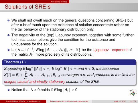
Solutions of SRE-s

We shall not dwell much on the general questions concerning SRE-s butafter a brief touch upon the existence of solution concentrate rather onthe tail behavior of the stationary distribution only.The negativity of the (top) Ljapunov exponent, together with some furthertechnical assumptions give the condition for the existence anduniqueness for the solution.Let Λ = inf

{ 1n ·E log‖A1 · . . . ·An)‖, n ∈ N

}be the Ljapunov - exponent of

the matrix An, more precisely of its distribution’s.

Theorem (1.)

Supposing E log+ ‖A1‖< ∞, E log+ |B1|< ∞ and Λ < 0, the sequence

X (t) = Bt +∞

∑k=1

At · . . . ·At−k+1Bt−k converges a.s. and produces in the limit the

unique, causal and strictly stationary solution of the SRE.

Notice that Λ < 0 holds if E log‖A1‖< 0


Non-Linear Models

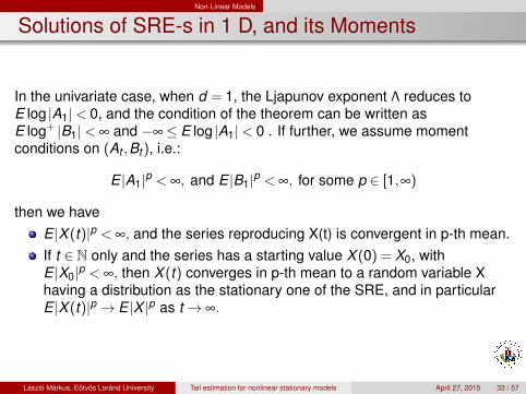
Solutions of SRE-s in 1 D, and its Moments

In the univariate case, when d = 1, the Ljapunov exponent Λ reduces toE log |A1|< 0, and the condition of the theorem can be written asE log+ |B1|< ∞ and −∞≤ E log |A1|< 0 . If further, we assume momentconditions on (At ,Bt ), i.e.:

E |A1|p < ∞, and E |B1|p < ∞, for some p ∈ [1,∞)

then we haveE |X (t)|p < ∞, and the series reproducing X(t) is convergent in p-th mean.If t ∈ N only and the series has a starting value X (0) = X0, withE |X0|p < ∞, then X (t) converges in p-th mean to a random variable Xhaving a distribution as the stationary one of the SRE, and in particularE |X (t)|p→ E |X |p as t → ∞.


Non-Linear Models

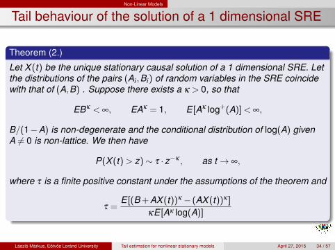
Tail behaviour of the solution of a 1 dimensional SRE

Theorem (2.)

Let X (t) be the unique stationary causal solution of a 1 dimensional SRE. Letthe distributions of the pairs (Ai ,Bi ) of random variables in the SRE coincidewith that of (A,B) . Suppose there exists a κ > 0, so that

EBκ < ∞, EAκ = 1, E [Aκ log+(A)] < ∞,

B/(1−A) is non-degenerate and the conditional distribution of log(A) givenA 6= 0 is non-lattice. We then have

P(X (t) > z)∼ τ ·z−κ , as t → ∞,

where τ is a finite positive constant under the assumptions of the theorem and

τ =E [(B + AX (t))κ − (AX (t))κ ]

κE [Aκ log(A)]


Non-Linear Models

Remarks on the tail behaviour

It is rather striking that no matter how the random pair (A,B) isdistributed, X (t) has Pareto-like tail.The constant κ is called the tail exponent, and τ is the tail index.The tail exponent does not always exist (and hence the tail index, too) .


Non-Linear Models

Regularly varying distributions

Let me remember you the definition of Regularly Varying distributions(RV)The X d-dimensional random vector has regularly varying distributionswith the regularity index κ ≥ 0 if there exists a sequence of real numbers(an), that

n ·P(|X |> t ·an,eX ∈ BS)−→ t−κQ(BS) n→ ∞

where eX denotes the unit vector to the direction of X and BS is a Borelset of the d-dimensional unit sphere S.In d = 1 dimension, accounting for the positivity of |X |, BS can only be thesingle point {+1} and n ·P(|X |> t ·an)−→ const · t−κ . Let e.g. an = n,then P(|X |> t ·n)∼ const

n · t−κ . This relation means that for sufficientlylarge n, i.e. if we start from far enough, the tail is of order t−κ , we haveParetian tails.


Non-Linear Models

Tail behaviour of the solution of a multidimensionalSRE

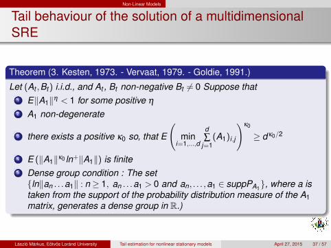
Theorem (3. Kesten, 1973. - Vervaat, 1979. - Goldie, 1991.)

Let (At ,Bt ) i.i.d., and At , Bt non-negative Bt 6= 0 Suppose that1 E‖A1‖η < 1 for some positive η

2 A1 non-degenerate

3 there exists a positive κ0 so, that E

(min

i=1,...,d

d∑

j=1(A1)i ,j

)κ0

≥ dκ0/2

4 E (‖A1‖κ0 ln+‖A1‖) is finite5 Dense group condition : The set{ln‖an . . .a1‖ : n ≥ 1, an . . .a1 > 0 and an, . . . ,a1 ∈ suppPA1}, where a istaken from the support of the probability distribution measure of the A1matrix, generates a dense group in R.)


Non-Linear Models

Tail behaviour of the solution of a multidimensionalSRE

Theorem (3. continued)

Under these assumptions the followings hold true1 There exists κ1 ∈ (0,κ0] a unique solution of the equation

0 = lim 1n · logE‖An · . . . ·A1‖κ1

2 There exists a unique, strictly stationary causal solution to the SRE .3 If further E |B|κ1 is finite, then X (t) is regularly varying with tail exponent

κ1.

Remark.Making use in one dimension that the independence yieldslogE‖An · . . . ·A1‖κ1 = n · logE |A1|κ1 , the first statement reduces to0 = logE |A1|κ1 that is equivalent to the equation 1 = E |A1|κ1 . So, thatabsolute moment is to be find which has its value equal to 1.


Non-Linear Models

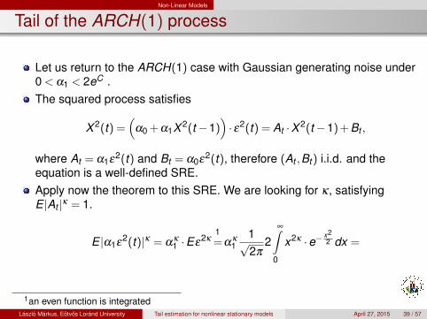
Tail of the ARCH(1) process

Let us return to the ARCH(1) case with Gaussian generating noise under0 < α1 < 2eC .The squared process satisfies

X 2(t) =(

α0 + α1X 2(t−1))· ε2(t) = At ·X 2(t−1) + Bt ,

where At = α1ε2(t) and Bt = α0ε2(t), therefore (At ,Bt ) i.i.d. and theequation is a well-defined SRE.Apply now the theorem to this SRE. We are looking for κ, satisfyingE |At |κ = 1.

E |α1ε2(t)|κ = α

κ1 ·Eε

2κ1=α

κ1

1√2π

2∞∫

0

x2κ ·e−x22 dx =

1an even function is integratedLaszlo Markus, Eotvos Lorand University Tail estimation for nonlinear stationary models April 27, 2015 39 / 57

Non-Linear Models

Tail of the ARCH(1) process, continued

Let us now integrate by substitution, let t = x2

2 , and with thatdx = 1

2√

2t·2dt = 1√

2tdt . The equality can be continued as follows

= ακ1

√2√π

∫∞

02κ · tκ ·e−t · 1√

2tdt

= (2α1)κ 1√π

∞∫0

t (κ+12 )−1 ·e−tdt

= (2α1)κ · 1√π·Γ(

κ +12

)= h(κ) = 1.

In the end we have arrived at the functional form for κ in terms of thegamma function as

(2α1)κ ·Γ(

κ +12

)=√

π.

In particular, κ = 1 is a good choice for α1 = 1, because√

π

2 = Γ(3

2

).


Non-Linear Models

Tail of the ARCH(1) process

h(κ) is a strictly convex decreasing function, so the equation has a uniquepositive solution. For the solution h(κ) = 1:

κ > 1, if α1 ∈ (0,1)

κ = 1, if α1 = 1κ < 1, if α1 ∈ (1,2eC)

The equation cannot be solved explicitly but numeric solutions are known asin the table below:

α1 0.1 0.3 0.5 0.7 0.9 1.0 1.5 2.0 2.5 3 3.5κ 13.24 4.18 2.37 1.59 1.15 1.0 0.54 0.31 0.17 0.075 0.007

Since we started from the equation for X 2, the tail exponent for the ARCH(1)process is exactly 2κ, prescribing a Paretian tail for the stationary solution ofthe ARCH(1) equation.


Non-Linear Models

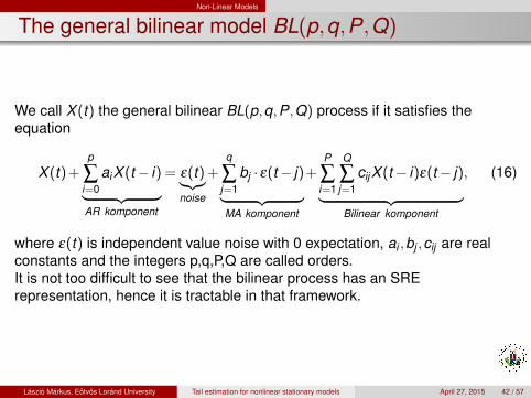
The general bilinear model BL(p,q,P,Q)

We call X (t) the general bilinear BL(p,q,P,Q) process if it satisfies theequation

X (t) +p

∑i=0

aiX (t− i)︸︷︷︸AR komponent

= ε(t)︸︷︷︸noise

+q

∑j=1

bj · ε(t− j)︸︷︷︸MA komponent

+P

∑i=1

Q

∑j=1

cijX (t− i)ε(t− j)︸︷︷︸Bilinear komponent

, (16)

where ε(t) is independent value noise with 0 expectation, ai ,bj ,cij are realconstants and the integers p,q,P,Q are called orders.It is not too difficult to see that the bilinear process has an SRErepresentation, hence it is tractable in that framework.


Non-Linear Models

The general bilinear model BL(p,q,P,Q)

Subba Rao(1981),Wang(1983), Gabr(1984), Tong(1990), Liu(1992),Pham(1993), Davis and Hsing (1995), Turkman and Turkman(1997), Igloiand Terdik (1999), Giraitis and Surgailis(2002) and others studied thestationarity, ergodicity, moments of various orders and distributionalproperties of the model.Liu and Brockwell gave in 1988 a quite general condition for the existenceand uniqueness of the stationary solution of the bilinear equation.


Non-Linear Models

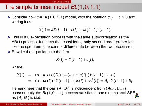
The simple bilinear model BL(1,0,1,1)

Consider now the BL(1,0,1,1) model, with the notation c1,1 = c > 0 andwriting it as :

X (t) = aX (t−1) + ε(t) + cX (t−1)ε(t−1).

This is a 0 expectation process with the same autocorrelation as theAR(1) process. It means that considering only second order propertieslike the spectrum, one cannot differentiate between the two processes.Rewrite the equation into the form

X (t) = Y (t−1) + ε(t),

where

Y (t) = (a + c · ε(t))X (t) = (a + c · ε(t))(Y (t−1) + ε(t))

= (a + cε(t)) ·Y (t−1) + (aε(t) + cε2(t)) = At ·Y (t−1) + Bt .

Remark here that the pair (At ,Bt ) is independent from (At−1,Bt−1)consequently the BL(1,0,1,1) process satisfies a one dimensional SRE,as (At ,Bt ) is i.i.d.


Non-Linear Models

The simple bilinear model, Gaussian Noise

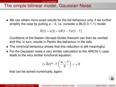
We can obtain more exact results for the tail behaviour only, if we furthersimplify the case by putting a = 0, i.e. consider a BL(0,0,1,1) model:

X (t) = ε(t) + cX (t−1)ε(t−1).

Conditions of the Kesten-Vervaat-Goldie theorem can then be verifiedand this, in turn, results in Pareto like behaviour in the tails.The nontrivial behaviour shows that this reduction is still meaningful.For the Gaussian noise a very similar calculation to the ARCH(1) caseleads to the very similar functional equation:

(√

2c)κ1 ·Γ(

κ1 + 12

)=√

π

that can be solved numerically, again.


Non-Linear Models

The simple bilinear model, Uniform Noise

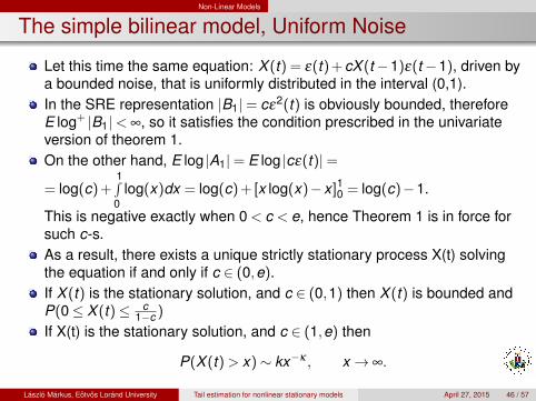
Let this time the same equation: X (t) = ε(t) + cX (t−1)ε(t−1), driven bya bounded noise, that is uniformly distributed in the interval (0,1).In the SRE representation |B1|= cε2(t) is obviously bounded, thereforeE log+ |B1|< ∞, so it satisfies the condition prescribed in the univariateversion of theorem 1.On the other hand, E log |A1|= E log |cε(t)|=

= log(c) +1∫0

log(x)dx = log(c) + [x log(x)−x ]10 = log(c)−1.

This is negative exactly when 0 < c < e, hence Theorem 1 is in force forsuch c-s.As a result, there exists a unique strictly stationary process X(t) solvingthe equation if and only if c ∈ (0,e).If X (t) is the stationary solution, and c ∈ (0,1) then X (t) is bounded andP(0≤ X (t)≤ c

1−c )

If X(t) is the stationary solution, and c ∈ (1,e) then

P(X (t) > x)∼ kx−κ , x → ∞.


Non-Linear Models

Simple bilinear model, Uniform Noise, Tail Exponent

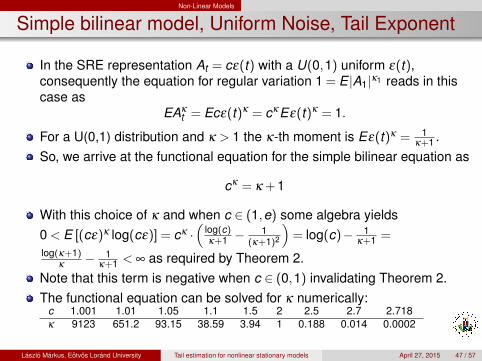
In the SRE representation At = cε(t) with a U(0,1) uniform ε(t),consequently the equation for regular variation 1 = E |A1|κ1 reads in thiscase as

EAκt = Ecε(t)κ = cκEε(t)κ = 1.

For a U(0,1) distribution and κ > 1 the κ-th moment is Eε(t)κ = 1κ+1 .

So, we arrive at the functional equation for the simple bilinear equation as

cκ = κ + 1

With this choice of κ and when c ∈ (1,e) some algebra yields0 < E [(cε)κ log(cε)] = cκ ·

(log(c)κ+1 −

1(κ+1)2

)= log(c)− 1

κ+1 =

log(κ+1)κ

− 1κ+1 < ∞ as required by Theorem 2.

Note that this term is negative when c ∈ (0,1) invalidating Theorem 2.The functional equation can be solved for κ numerically:

c 1.001 1.01 1.05 1.1 1.5 2 2.5 2.7 2.718κ 9123 651.2 93.15 38.59 3.94 1 0.188 0.014 0.0002


Non-Linear Models

Essential Supremum and Infimum

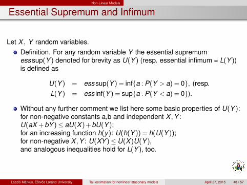
Let X , Y random variables.Definition. For any random variable Y the essential supremumess sup(Y ) denoted for brevity as U(Y ) (resp. essential infimum = L(Y ))is defined as

U(Y ) = ess sup(Y ) = inf{a : P(Y > a) = 0}, (resp.L(Y ) = ess inf(Y ) = sup{a : P(Y < a) = 0}).

Without any further comment we list here some basic properties of U(Y ):for non-negative constants a,b and independent X ,Y :U(aX + bY )≤ aU(X ) + bU(Y );for an increasing function h(y): U(h(Y )) = h(U(Y ));for non-negative X ,Y : U(XY )≤ U(X )U(Y ),and analogous inequalities hold for L(Y ), too.


Non-Linear Models

Simple bilinear model, Uniform Noise, BoundedDistribution

Let 0 < c < 1. We have X (t) > 0 since ε(t) > 0, too.The coefficients of the SRE representation are At = cε(t), Bt = cε2(t),and remember, the solution can be given as

X (t) = Bt +∞

∑k=1

At · . . . ·At−k+1Bt−k .

By virtue of the mentioned elementary properties of U(.) and the fact thatU(ε(t)) = U(ε2(t)) = 1 the upper bound can be estimated as

U(X (t)) ≤ U(cε2(t)) +

∞

∑k=1

U(cε(t)) · . . . ·U(cε(t−k + 1)U(cε2(t−k))≤

≤ c +∞

∑k=1

ck+1 =c

1−c.

This proves the assertion on the boundedness from above of the stationarydistribution, when 0 < c < 1. The lower bound can be proven similarly.


Non-Linear Models

AR(1) model, generated by ARCH(1) Noise

Consider the equation:

X (t) = αX (t−1) +√

α0 + α1X (t−1)2ε(t), (17)

where α ∈ R,α0,α1 > 0, and the starting value, X (0) is independent ofε(t), t ≥ 0 guaranteeing causality of the stationary solution.The solution is evidently a homogeneous Markov chain with R as its statespace.It does not have an SRE representation, however.Suppose the noise distribution

1 has full support: R,2 is symmetric,3 has a Lebesgue density f(z),4 has finite second moment.5 the density f(z) is monotonously decreasing in the positive halfline,


Non-Linear Models

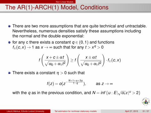
The AR(1)-ARCH(1) Model, Conditions

There are two more assumptions that are quite technical and untractable.Nevertheless, numerous densities satisfy these assumptions includingthe normal and the double exponential:for any c there exists a constant q ∈ (0,1) and functionsf±(c,x)→ 1 as x → ∞ such that for any t > xq > 0

f

(x + c±αt√

α0 + α1t2

)≥ f

(x±αt√α0 + α1t2

)· f±(c,x)

There exists a constant η > 0 such that

f (z) = o(z−N+1+η+3q

1−q ), as z→ ∞

with the q as in the previous condition, and N = inf {u : E |√α1ε|u > 2}


Non-Linear Models

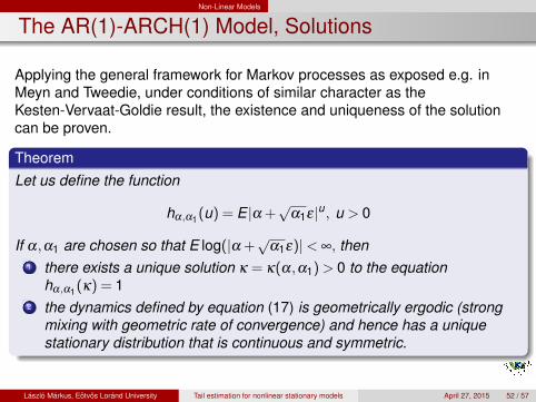
The AR(1)-ARCH(1) Model, Solutions

Applying the general framework for Markov processes as exposed e.g. inMeyn and Tweedie, under conditions of similar character as theKesten-Vervaat-Goldie result, the existence and uniqueness of the solutioncan be proven.

TheoremLet us define the function

hα,α1(u) = E |α +√

α1ε|u, u > 0

If α,α1 are chosen so that E log(|α +√

α1ε)|< ∞, then1 there exists a unique solution κ = κ(α,α1) > 0 to the equation

hα,α1(κ) = 12 the dynamics defined by equation (17) is geometrically ergodic (strong

mixing with geometric rate of convergence) and hence has a uniquestationary distribution that is continuous and symmetric.


Non-Linear Models

The AR(1)-ARCH(1) Model, Tail Behavior (theoremcontinued)

TheoremFor the right tail of the distribution function

P(X (t) > z)∼ l(z) ·z−κ

with the same κ as in the previous statement, and with the slowly varyingfunction l(z).If we choose N so that E |√α1ε|N > 2 then the N-th moment of the stationarydistribution is infinite EX (t)N = ∞.

For the values of κ = κ(α,α1) we find the following relationship:1 κ > 2, if α2 + α1E(ε)2 < 1 Thus, X (t) has finite 2nd moment.2 κ = 2, if α2 + α1E(ε)2 = 13 κ < 2, if α2 + α1E(ε)2 > 1


Non-Linear Models

The AR(1)-ARCH(1) Model, Remarks

Remarks. I wish to stress that although the result is very much similar to theones deduced from Kesten and Goldie, it is necessary to use differenttechnique here, a Tauberian theorem is the key the so called Drasin-Sheatheorem. It is noteworthy to mention that all results so far found heavy tailbehaviour. Little is known about exponential or subexponential speed in thedecay of the tails.


Non-Linear Models

References

Bingham, N. H., Goldie, C. M. and Teugels, J. L. (1987). Regular Variation. Cambridge Univ.Press.

Bollerslev, T. (1986). Generalized autoregressive conditional heteroscedasticity. J.Econometrics 31 307-327.

Borkovec, M. (2000). Extremal behavior of the autoregressive process with ARCH(1) errors.Stochastic Process Appl. 85 189-207.

Davis, R. and Resnick, S.I. (1985) Limit theory for moving averages of random variableswith regularly varying tail probabilites. Ann. Probab., 13, 179-195.

Diebolt, J. and Guegan, D. (1990). Probabilistic properties of the general nonlinearMarkovian process of order one and applications to time series modelling. TechnicalReport, 125, L.S.T.A., Paris 6.

Embrechts, P., Kluppelberg, C. and Mikosch, T. (1997). Modelling Extremal Events forInsurance and Finance. Springer, Berlin.

Engle, R. F. (1982). Autoregressive conditional heteroscedasticity with estimates of thevariance of U.K. inflation. Econometrica 50 987-1007.

Goldie, C. M. (1991). Implicit renewal theory and tails of solutions of random equations.Ann. Appl. Probab. 1 126-166.

Kesten, H. (1973). Random difference equations and renewal theory for products of randommatrices. Acta Math. 131 207-248.


Non-Linear Models

Some references, continued

Klueppelberg, C. and S. Pergamenchtchikov, 2007, Extremal Behaviour of Models withMultivariate Random Recurrence Representation, Stochastic Processes and theirApplications, 117, 432-456.

Maercker, G. (1997). Statistical inference in conditional heteroskedastic autoregressivemodels. Dissertation, Univ. Braunschweig.

Meyn, S. P. and Tweedie, R. L. (1993). Markov Chains and Stochastic Stability. Springer,London.

Rootzen, H. (1986) Extreme value theory for moving averages. Ann. Probab., 14, 612-652.

Tong, H. (1990). Nonlinear Time Series: A Dynamical System Approach. Oxford Univ.Press.

Tweedie, R. L. (1983b). The existence of moments for stationary Markov chains. J. Appl.Probabab. 20 191-196.

Vervaat, W. (1979). On a stochastic difference equation and a representation ofnonnegative infinitely divisible random variables. Adv. Appl. Probab. 11 750-783.


Non-Linear Models

Thank you for your attention!


laszl´ o m´ arkus´ department of probability th

Documents