1

1.6 METHODS OF ANALYSING VARIABILITY

Lars Gottschalk

Department of Geosciences, University of Oslo, Norway

Keywords: Random variable, - process, - vector; persistence; time series; integral scale;

distribution function; correlation function; semivariogram; Karhunen- Loève expansion;

Summary

In an introductory part basic concepts from probability theory, and specifically from the

theory of random processes, are introduced as a basis for the characterization of

variability of hydrological time series, space processes and time-space processes. A

partial characterization of the random process under study is adopted in accordance with

three different schemes:

i) Characterization by distribution function (one dimensional),

ii) Second moment characterization, and

iii) Karhunen-Loève expansion i.e. a series representation in terms of random

variables and deterministic functions of a random process.

Chapter follows the same division into three major sections. In the first one distribution

functions of frequent use in hydrology are shortly described as well as the flow duration

curve. The treatment of second order moments includes covariance/correlation functions,

spectral functions and semivariograms. They allow establishing the structure of the data

in space and time and its scale of variability. They also give the possibility of testing

basic hypothesis of homogeneity and stationarity. By means of normalization and

standardization data can be transformed into new data sets owing these properties.

The section on Karhunen-Loève expansion includes harmonic analysis, analysis by

wavelets, principal component analysis, and empirical orthogonal functions. The

characterization by series representation in its turn assumes homogeneity with respect to

the variance-covariance function. It is as such a tool for analyzing spatial-temporal

variability relative to the first and second order moments in terms of new sets of common

orthogonal random functions.

2

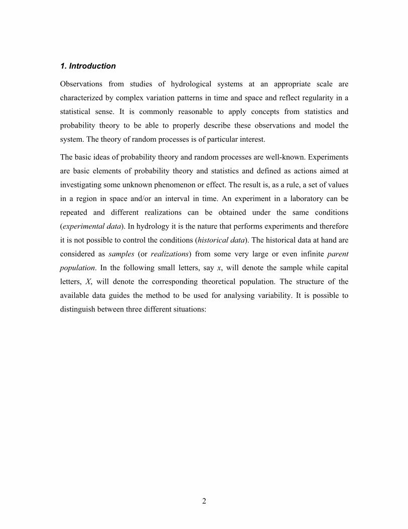
1. Introduction

Observations from studies of hydrological systems at an appropriate scale are

characterized by complex variation patterns in time and space and reflect regularity in a

statistical sense. It is commonly reasonable to apply concepts from statistics and

probability theory to be able to properly describe these observations and model the

system. The theory of random processes is of particular interest.

The basic ideas of probability theory and random processes are well-known. Experiments

are basic elements of probability theory and statistics and defined as actions aimed at

investigating some unknown phenomenon or effect. The result is, as a rule, a set of values

in a region in space and/or an interval in time. An experiment in a laboratory can be

repeated and different realizations can be obtained under the same conditions

(experimental data). In hydrology it is the nature that performs experiments and therefore

it is not possible to control the conditions (historical data). The historical data at hand are

considered as samples (or realizations) from some very large or even infinite parent

population. In the following small letters, say x, will denote the sample while capital

letters, X, will denote the corresponding theoretical population. The structure of the

available data guides the method to be used for analysing variability. It is possible to

distinguish between three different situations:

3

0

100

200

300

400

500

600

700

800

900

1800 1820 1840 1860 1880 1900 1920 1940

year

Stea

mflo

w [m

3 /s]

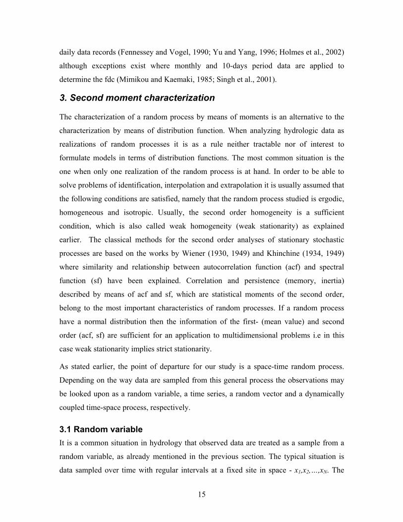
Figure.1 Time series: Streamflow of the Göta River at Sjötorp, Sweden 1807-1938.

i. An observation point in space is fixed and only the development in time is

observed at this point, as illustrated in Fig. 1, where the annual streamflow for the

Göta River for the period 1807-1938 is shown. This is referred to as a time series

xk=x(tk), k=1,...,N, where tk denotes the (regular) observation points in time (here

years) and N is the number of observations (in the example N=131). The process

is characterized by an active and inherent dynamic uncertainty, the properties in

different points change with time in a random manner. In the general case the

order in which time series is sampled is of outmost importance as the temporal

fluctuations show persistence i.e. adjacent observations show dependence. The

opposite situation when data are independent and can be reshuffled without loss

of information is an important special case.

4

p47

p45

p43

p41

GPR profiles

p41p43p45p47

MoreppenN

10 m

Figure.2 Space process: The geological structure of the top layer of the Gardemoen delta

deposit at Moreppen (Norway) as reflected by georadar measurements (Ground

Penetrating Radar (GPR) signals for 4 profiles. The strong reflectors in the dipping foreset unit

are from silty layers with high soil moisture content. Yellow and green colours reflect drier sand.

ii. The second situation – a space process xi=x(ui), i=1,...,M- is illustrated by

georadar measurements reflecting the geological structure of the top layer of the

Gardemoen delta deposit at Moreppen (Norway) along transects of some 10th of

meters. ui denotes the position in space of the i-th measurement, of totally M. In

the example observations are made at a regular grid in space. More common is the

case of spatial measurements from an irregular observation network. It may be

assumed in this case that the changes over time of the system are small (at a

human time scale). The uncertainty in the description of the properties of a

disordered system, for which the development in time does not matter, is of

passive nature. Though the changes in time of a characteristic at a given position

might be negligible, its value is unknown until it is measured. Measurements in

5

all possible points are, as a rule, neither feasible nor economic, and the

information value is lowered by the measurement errors as well. Persistence in

data is also of relevance for spatial data i.e. the order in which they are sampled in

the two dimensional space is of vital importance.

Figure.3 Time-space process: Estimated streamflow of the Rhône River for the twelve

months of the year (From Sauquet and Leblois, 2001) .

iii. Fig. 3 offers an attempt to illustrate of the most general case showing the space-

time development of streamflow (monthly values) along the different branches of

the Rhône River (French part). In reality, observations of such a time-space

process xik=x(ui,tk), i=1,...,M; k=1,...,N represent measurements in discrete

irregular points along the river network at discrete regular times (and not as the

6

fully reconstructed space-time development as in Fig. 3), i.e. a vector of data

where columns represent different points in space and rows time. These

observations are used to get an idea about the pattern of variation of the whole

system by means of reconstructing the past development in time and space and/or

forecasting the future.

7

Figure 4. Observed precipitation at Blindern (Oslo) with 5 different time resolutions 2

minutes, 1 hour, 1 day, 1 month and 1 year.

8

The scale problem is fundamental in all description and modelling of time-space

processes. A phenomenon that seems to contain mainly deterministic elements in a micro

scale might at a larger scale demonstrate characteristics that vary much and demand a

probabilistic approach for their description. At a still larger scale (macro scale) the same

structure can appear to be a part of an object that can be described by its mean value or

by classes. Variation of precipitation intensity at annual and daily time scales seems to

behave totally at random, while at a finer time scale (minutes) this variation assumes a

dynamically varying pattern (Fig 4). At the monthly scale a seasonal variation might be

present. In other words, there is, as a rule, the lower and the upper boundary for the

variation range (distance or time) within which a model for characterization of the

patterns of variations has a practical value. This is the point of departure for the

application of classical theory of random processes in hydrology which has been mainly

applied to study stationary (time independent) random processes like annual or sub-

monthly quantities (upper three graphs, and lower graph in Fig. 4). Possible large scales

elements like “trends” and “periods” were looked upon as “deterministic”, and as such

identified and subtracted from the original data (e.g. Hansen 1971, Yevjevich 1972). This

perspective contrasts with the current view accepting “... irregularly changes, for

unknown reasons on all time scales” (National Research Council, 1991). Random process

models need to be changed accordingly. The scale problem is of course not only limited

to processes in time. Referring to the geological structure in Fig. 2 the patterns of

variability and its character will change drastically both when going down in scale as

when going up. The topic of scale is further developed in Chapters hsa005 and hsa008).

Let us turn back to probability theory terminology and continue formalizing the

description of the outcome of an experiment. In the elementary case the population is

described in terms of a random variable and in more complex situations as a random

process (random field). Our basic model is illustrated in Fig. 3, where each point in the

sample space u ∈Ω (points along rivers) maps into a time function X(u,t). A point uk in

space can be specified which results in a random process in time, a time series,

X(t)=Xk(t), like the one shown in Fig. 1. If the data of the series fulfil the condition of

having an independent identical distribution (i.i.d.) they can be treated as a sample of a

random variable X. Only in this latter case the one dimensional probability distribution

9

FX(x) will give a complete characterization of X. The time t=ti can be frozen which leads

to a random process in space only X(u)=Xi(u), illustrated in Fig. 2. Also in this case a one

dimensional distribution describes variations across space. The i.i.d. condition should, of

course, be fulfilled to give a complete description.

Many important characteristics of random processes viz. homogeneity (stationarity),

isotropy and ergodicity, permit a more effective use of the limited data amount available

for estimation of important properties of the process. The strict definitions of these

characteristics can be formulated with the help of the multivariate (M-dimensional)

distribution function FM(x) (abbreviated df). A random process is called homogeneous if

all multivariate distributions do not change with the movement in the parameter space

(translation, not rotation). This implies that all probabilities depend on relative and not

absolute positions of points in the parameter space. The term "stationary" instead of

homogeneous is usually used for one-dimensional random processes (time series) i.e. the

df does not change with time. A process is called isotropic if the multivariate distribution

function remains the same even when the constellation of points is rotated in the

parameter space. A random process is ergodic if all information about this multivariate

distribution (and its parameters) is contained in a single realization of the random field. It

is important to note that this property is also related to the characteristic scale of

variability of the process. If the process is observed over a time interval (or region in

space), which in its extension is of the same order of magnitude as the characteristic scale

(or smaller), the estimate of the variability of the process will by necessity be negatively

biased. The process will not be able to show its whole range of patterns of variability. A

rule of thumb has been to say that a process needs to be observed for a period of time that

is at least ten times the characteristic scale of the process, in order to eliminate the

negative bias in the variance. In times when environmental and climate change are in

focus and accepting that the process shows variability on a range of scales, the dilemma

related to the ergodicity problem is obvious. Do the observed data reveal the real

variability of the natural processes under study? In Chapter hsa008 this topic is brought

further and the process scale related to the natural variability is confronted with the

measurement scale, defined in terms of extent (coverage), spacing (resolution) and

support (integration volume (time) of a data set).

10

The parameter space of a random process X(u,t) in the general case includes an unlimited

and infinite number of points. Characterization by means of distributions functions is

therefore only of a theoretical value. When complex variation patterns are concerned, a

possibility of a direct estimation of the underlying multivariate distribution function is not

tractable. The conventional way of handling this difficulty is to accept a partial

characterization. The two most widely used are:

i) Characterization by distribution function (one dimensional), and

ii) Second moment characterization.

In a characterization by the distribution function only the first order probability density is

specified. In a characterisation by distribution function in the general case a multivariate

distribution would be needed for a complete characterisation. The one dimensional

distribution constitutes in this case the marginal distribution of the data. The flow

duration curve (fdc) widely used in hydrology is a good example. In a second-moment

characterization only the first and second moments of the process are specified i.e. mean

values, variances and covariances. Random processes, which are postulated to be

homogenous (stationary), in practice satisfy this condition only in a weak sense and not

strongly, which means that they possess this property only with respect the to the first and

second order moments (weak homogeneity, weak stationarity). A further possibility is to

apply

iii) Karhunen-Loève expansion i.e. a series representation in terms of random

variables and deterministic functions of a random process.

The deterministic functions can either be postulated as for harmonic analysis and analysis

by wavelets or they can be determined from the data themselves by analysis in terms of

empirical orthogonal functions (eof) or principal components (pca).

In this chapter these three ways for representation of a random process will be followed,

thus defining three methods for describing variability of hydrologic variables. The

development of relations between variability and scale is treated in Ch. hsa008, although

some aspects of the problem are touched upon here as well. Before going into a detailed

statistical analysis the importance of "looking" at data should be stressed. A visual

11

inspection of graphical plots of the observed data like those shown in Figs. 1, 2 and 4, is a

natural point of departure when analysing variability. In our age of nearly unlimited

computing power this visual graphical data exploration is becoming increasingly

important. A further step is an exploratory data analysis, where different hypotheses

concerning the structure of the data are tested (Tukey, 1977).

2. Characterization by distribution function

Restricting ourselves to the one-dimensional case, the basic problem is the following:

find a distribution function (df) FX(x) (probability density function fX(x), pdf), which is a

good model for the parent data x1,x2,…,xN. From probability theory it is well known that

this distribution only gives a full description of phenomena in case data can fulfil the

condition of being independent identically distributed (i.i.d.). In many applications in

hydrology the i.i.d.-assumption is rather postulated than really tested and the one

dimensional distribution is to be interpreted as a partial characterisation (the marginal

distribution function of a multivariate one). Anyhow this marginal distribution might be a

proper tool to study the data. The application of the normal distribution for frequency

analysis of runoff data by Hazen (1917) symbolises the start of the fitting a theoretical

distribution to observed data in hydrology. Somewhat later it became obvious that the

river runoff distribution is not symmetrical and also the gamma distribution was

introduced in hydrological analysis (Foster, 1923 and 1924; Sokolovskij, 1930).

Important benchmarks in the utilisation of probability theory and statistical methods in

hydrology were the developments by Kritskij and Menkel (1946) who suggested a

transformation of the gamma distribution and Chow (1954) who introduced the log-

normal distribution. Fig. 5 illustrates the change in the distribution (pdf) of precipitation

with changing time step for data from to two stations in Norway, starting from a highly

skewed distribution for daily data, to a lognormal shape for monthly data and ending with

a symmetric normal distribution for annual data. This example provides an illustration of

the Central Limit Theorem in Statistics that states that the distribution of a sum of

random variables converges to normal distribution as the number of elements in the sum

approaches infinity. How quickly the sum converges (and also if it converges) depends

on how well certain assumptions are fulfilled. Still it is important to note that data follow

12

statistical laws and that knowledge of these laws helps when analysing and interpreting

results as well as in choosing an appropriate model. The list of theoretical distributions

applied to hydrological data since Hazen can be made very long. A remark might be that

the advantage of using a more complex distribution with many parameters instead of the

classical ones (the normal, the gamma, the lognormal) is usually minor in relation to the

small data samples commonly available and thereby related uncertainty.

13

Figure 5. The distribution (pdf) of rainfall at two Norwegian rainfall stations (Skjåk and

Samnanger) for three different durations 1 day, 1 month and 1 year.

14

The flow-duration curve (fdc) represents the relationship between the magnitude and

frequency of daily, weekly, monthly (or some other time interval) of streamflow for a

particular river basin, providing an estimate of the percentage of time a given streamflow

was equalled or exceeded over a historical period (Vogel and Fennessey , 1994). The fdc

has a long tradition of application for applied problems in hydrology. The first paper on

this topic, in accordance with Foster (1933), is the one published by Herschel in 1878.

The interpretation of fdc by Foster is: “(Frequency and) duration curves may be

considered as forms of probability curves, showing the probability of occurrence of items

of any given magnitude of the data.” In this respect a fdc is a plot of the empirical

quantile function Xp, i.e. the p-th quantile or percentile of streamflow for a certain

duration versus exceedance probability p, where p is defined by:

( )xFxXPp X−=≤−= 11 (1)

Foster sees two distinct uses of the fdc: 1) if treated as a probability curve, it may be used

to determine the probability of occurrence of future events; and 2) it can be used merely

as a conventional tool for studying of the data. Mosley and McKerchar (1992) look at the

problem from a different point of view: “It (a flow duration curve) is not a probability

curve, because discharge is correlated between successive time intervals, and discharge

characteristics are dependent on season of the year. Hence the probability that discharge

on a particular day exceeds a specific value depends on the discharge on proceeding days

and on the time of the year”. Indeed the fdc gives a static and incomplete description of a

dynamic phenomenon in terms of cumulative frequency of discharge. To have a complete

description it is necessary to turn over to a multivariate distribution, which defines the

parent distribution of the data. Anyhow the marginal distribution of this parent

distribution is the fdc. It is a natural point of departure when analysing streamflow data,

which is evident from its wide practical application (Foster, 1933; Vogel and Fennessey,

1995; Holmes et al., 2002).

Foster in his original paper compared daily, monthly and annual fdcs and recognised the

fact that the differences between the curves for different durations (time scale) changed

with the type of river basins. Searcy (1959) performed a similar comparison. With

present computer technology it is usually taken for granted that the fdc is founded on

15

daily data records (Fennessey and Vogel, 1990; Yu and Yang, 1996; Holmes et al., 2002)

although exceptions exist where monthly and 10-days period data are applied to

determine the fdc (Mimikou and Kaemaki, 1985; Singh et al., 2001).

3. Second moment characterization

The characterization of a random process by means of moments is an alternative to the

characterization by means of distribution function. When analyzing hydrologic data as

realizations of random processes it is as a rule neither tractable nor of interest to

formulate models in terms of distribution functions. The most common situation is the

one when only one realization of the random process is at hand. In order to be able to

solve problems of identification, interpolation and extrapolation it is usually assumed that

the following conditions are satisfied, namely that the random process studied is ergodic,

homogeneous and isotropic. Usually, the second order homogeneity is a sufficient

condition, which is also called weak homogeneity (weak stationarity) as explained

earlier. The classical methods for the second order analyses of stationary stochastic

processes are based on the works by Wiener (1930, 1949) and Khinchine (1934, 1949)

where similarity and relationship between autocorrelation function (acf) and spectral

function (sf) have been explained. Correlation and persistence (memory, inertia)

described by means of acf and sf, which are statistical moments of the second order,

belong to the most important characteristics of random processes. If a random process

have a normal distribution then the information of the first- (mean value) and second

order (acf, sf) are sufficient for an application to multidimensional problems i.e in this

case weak stationarity implies strict stationarity.

As stated earlier, the point of departure for our study is a space-time random process.

Depending on the way data are sampled from this general process the observations may

be looked upon as a random variable, a time series, a random vector and a dynamically

coupled time-space process, respectively.

3.1 Random variable It is a common situation in hydrology that observed data are treated as a sample from a

random variable, as already mentioned in the previous section. The typical situation is

data sampled over time with regular intervals at a fixed site in space - x1,x2,…,xN. The

16

situation of data sampled on a regular or irregular network in space at a fixed time is also

of interest, e.g. snow or soil moisture surveys.

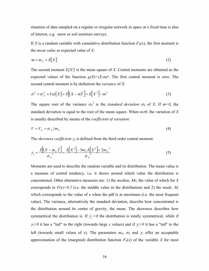
If X is a random variable with cumulative distribution function FX(x), the first moment is

the mean value or expected value of X:

[ ]XEmm X == (2)

The second moment E[X²] is the mean square of X. Central moments are obtained as the

expected values of the function g(X)=(X-m)n. The first central moment is zero. The

second central moment is by definition the variance of X:

[ ] ( )[ ] [ ] 22222 mXEmXEXVarX −=−===σσ (3)

The square root of the variance σX2 is the standard deviation σX of X. If m=0, the

standard deviation is equal to the root of the mean square. When m≠0, the variation of X

is usually described by means of the coefficient of variation:

XXX mVV σ== (4)

The skewness coefficient γ1 is defined from the third order central moment:

( )[ ] [ ] [ ]3

323

3

3

123

X

XX

X

X mXEmXEmXEσσ

γ +−=

−= (5)

Moments are used to describe the random variable and its distribution. The mean value is

a measure of central tendency, i.e. it shows around which value the distribution is

concentrated. Other alternative measures are: 1) the median, Me, the value of which for X

corresponds to F(x)=0.5 (i.e. the middle value in the distribution) and 2) the mode, M,

which corresponds to the value of x when the pdf is at maximum (i.e. the most frequent

value). The variance, alternatively the standard deviation, describe how concentrated is

the distribution around its centre of gravity, the mean. The skewness describes how

symmetrical the distribution is. If γ1 =0 the distribution is totally symmetrical, while if

γ1>0 it has a "tail" to the right (towards large x values) and if γ1<0 it has a "tail" to the

left (towards small values of x). The parameters mX, σX and γ1 offer an acceptable

approximation of the (marginal) distribution function FX(x) of the variable X for most

17

applications in hydrology. In the applied case mX, σX and γ1 are substituted by the

corresponding sample moments 1,, gsx , respectively:

( )∑=

=N

kktx

Nx

1

1 (2’)

( )∑=

−=N

kkX xtx

Ns

1

222 1 (3’)

( ) ( ) 3

1

2

1

31 2131 sxtx

Nxtx

Ng

N

kk

N

kk

+−= ∑∑

==

(5’)

The moments of the sample are accompanied with sampling errors (standard errors) and

biases. The well known formula for the standard error of the mean is:

NXX σσ =&&& (6)

or as estimated from the sample:

Nss XX =&&& (6’)

The standard error of the mean is not dependent on the distribution of the population.

Standard errors of higher order moments are related to the theoretical distribution

(Kendall et al., 1987). The moments developed here are obviously of the same

importance whether or not the necessary i.i.d. conditions are satisfied. On the other hand

it is important to clearly state whether the moments of the one dimensional distribution of

a random variable are considered or the moments of the marginal distribution of a

random process. In the latter case the standard errors and the bias of the moments are

related to the structure (covariance function) of the data (see 3.2 below). The classical

methods for statistical tests for random variables are thus not directly applicable in this

latter case.

3.2 Time series A time series is a sequence of data are sampled over time with regular intervals at a fixed

site in space or data are sampled along a line in space at regular intervals at a fixed time –

x(t1),x(t2),…,x(tN) like in Fig. 3.1. The difference, compared to the previous section, is

18

that the order in which data are sampled in the parameter space t1, t2,...,tN is here of vital

importance. The two first order moments mX and σX determine the marginal distribution

function FX(x) of the random process X(t), like in the case of a random variable.

However, for a random process a descriptor of the random structure of this process needs

to be added and the autocovariance function (acf) (the second order mixed moment)

determines this structure as an acceptable approximation. The covariance B(t,t’) of the

state of a random process between two different points in time X(t) and X(t’) defines this

autocovariance function (of t and t’):

( ) ( ) ( ) ( )[ ] ( ) ( )[ ] ( ) ( )tmtmtXtXEtXtXCovttBttB X ′−′=′=′=′ ,,,, (7)

Similarly, the autocorrelation function is defined by:

( ) ( ) ( )( ) ( )tt

ttBtttt X ′′

=′=′σσ

ρρ ,,, (8)

which is the correlation coefficient between X(t) and X(t’). A weakly stationary random

process has the following properties:

( )[ ] ( ) mtmtXE == ,

( )[ ] ( )[ ]( )∞<tXVartallforexiststXVar , , and (9)

( ) ( ) ( )τBttBttB =′−=′,

τ=|t-t’| describes the relative distance between the two points in time. The autocovariance

function, as well as the autocorrelation function, depend therefore only on relative

positions in time, and not absolute ones. A simple measure of the scale of variability can

be defined as the integral under the autocorrelation for τ>0, the integral scale θX of a

stationary process i.e.:

( )∫∞

=0

ττρθ dX (10)

For stationary processes, a characterization using the spectral function (sf) SX(f), where f

is the frequency, is equivalent to the covariance function characterization:

19

( ) ( )∫∞

∞−

= ττ τπ deBfS fiXX

2 (11)

and

( ) ( )∫∞

∞−

−= dfefSfB fiXX

τπ2 (12)

These two equations are usually referred to as the Wiener-Kinchine relations.

The stationarity assumption eq. (9), which also is the theoretical background for the

derivation of the Wiener-Kinchine equations, demands finite variance. The existence of a

process with variation at many scales might violate this assumption theoretically. The

demand of a weak stationarity is then too strong. An alternative is then to put the demand

of stationarity on the differences [X(ti)-X(tj)], i.e. that its mean value is constant and

variance is finite and independent on absolute position. This means mathematically:

( ) ( )[ ] 0=− ji tXtXE , and (13)

( ) ( )[ ] ( ) ( )( )[ ] ( ) ( )τγγ 22 212 =−=−=− tttXtXEtXtXVar jiji (14)

The conditions above are called the intrinsic hypothesis. In classical works on turbulence

and also in meteorology the function eq. (14) is named structure function (Kolmogorov,

1941). It is also called variogram (Matheron, 1965) and γ(τ) is accordingly called

semivariogram (sv), i.e.:

( ) ( ) ( )( )[ ]2212

1 tXtXE −=τγ (15)

The intrinsic assumption is more general than the demand for second order stationarity

(weak stationarity). If the condition for weak stationarity is satisfied, i.e. the variance

exists and equals B(0), the following relation between the semivariogram and covariance

functions can be established:

( ) ( ) ( )ττγ BB −= 0 (16)

The semivariogram is not commonly used for analysing temporal data in hydrology. It is

treated more in detail in the section for the analysis of spatial data below.

20

-0.5

-0.4

-0.3

-0.2

-0.1

0

0.1

0.2

0.3

0.4

0.5

0.6

0.7

0.8

0.9

1

0 1 2 3 4 5 6 7 8 9 10 11 12 13 14 15 16 17 18 19 20

years

auto

corr

elat

ion

-0.5

-0.4

-0.3

-0.2

-0.1

0

0.1

0.2

0.3

0.4

0.5

0.6

0.7

0.8

0.9

1

0 12 24 36 48 60 72 84 96 108 120 132 144 156 168 180 192

months

auto

corr

elat

ion

0

1000

2000

3000

4000

5000

6000

7000

8000

9000

10000

0 1 2 3 4 5 6 7 8 9 10 11 12 13 14 15 16 17 18 19 20

years

sem

ivar

iogr

am

0

2000

4000

6000

8000

10000

12000

14000

0 12 24 36 48 60 72 84 96 108 120 132 144 156 168 180 192

months

sem

ivar

iogr

am

1000

10000

100000

0 0.05 0.1 0.15 0.2 0.25 0.3 0.35 0.4 0.45 0.5

frequency

log-

spec

trum

10000

100000

1000000

0 0.05 0.1 0.15 0.2 0.25 0.3 0.35 0.4 0.45 0.5

frequency

log-

spec

trum

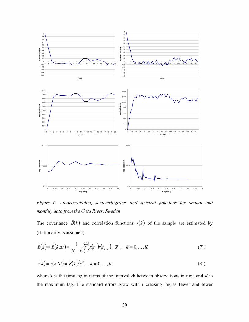
Figure 6. Autocorrelation, semivariograms and spectral functions for annual and

monthly data from the Göta River, Sweden

The covariance ( )kB and correlation functions ( )kr of the sample are estimated by

(stationarity is assumed):

( ) ( ) ( ) ( ) KkxtxtxkN

tkBkBkN

kkjj ,,0;1ˆˆ 2

1K=−

−=∆= ∑

−

=+ (7’)

( ) ( ) ( ) KkskBtkrkr ,,0;ˆ 2 K==∆= (8’)

where k is the time lag in terms of the interval ∆t between observations in time and K is

the maximum lag. The standard errors grow with increasing lag as fewer and fewer

21

observations are available for estimation. A rule of thumb is to set K=0.1*N as only a few

foremost terms can be known with some acceptable confidence. An estimate of the

sample semivariogram ( )kγ when data are available at regular time intervals is

( ) ( ) ( ) ( ) ( )( ) KktxtxkN

tkkkN

kkjj ,,0;

21ˆˆ

2

1K=−

−=∆= ∑

−

=+γγ . (15’)

The estimation of the sample spectral function is more complicated. There exist two

principal approaches. One relies on the Wiener-Khinchine equation (11) and the spectral

function is calculated from the sample autocorrelation function by numerical integration

of this equation. The other is founded on an expansion of the observed data in terms of

Fourier series resulting in a so called periodogram. Very fast algorithms are available i.e.

FFT (Fast Fourier Transform) for this purpose. The highest frequency that can be

represented by the sample spectral function is the so called Nyquist frequency fN=1/(2∆t).

Low frequency components with wavelengths in the order of magnitude of the total

period of observations (T=N*∆t) or larger are estimated with poor accuracy and are

numerically filtered out. The sample spectrum thus cover frequencies for the range

( )tfTNK ∆<< 211 , where K as before is the truncation level for the time lag. Fig. 6

illustrates the estimated acf, sv and sf of the discharge data from the Göta River, Sweden

(Fig.1). This river drains a large lake Vänern, which explains the very high

autocorrelation in these series both for the annual and the monthly time step. A seasonal

variation pattern as well as a strong between year variability is noted. Note that the

Nyquist frequency of 0.5 in the lower left diagram for annual data relates to a period of 2

years while the corresponding lower right diagram for monthly data relates to a period of

2 months.

How far can the information about the variability of the studied process contained in the

acf, sv and sf be interpreted i.e. which model can be applied? This question is linked to

the discussion in the introductory section about the existence of variability in data across

a range of scales. A traditional approach, as already commented on, has been to divide

the variability in time series into two parts viz. one related to deterministic variations and

the remaining one to random fluctuation. The goal in this approach has been to be able to

describe the random part by a stationary random process. The deterministic part in its

22

turn may be described by long term trends as well as purely periodic fluctuations. A

common model for this case would look as follows:

( ) ( )tSPDtX ttt ε++= (17)

where Dt denotes the trend, Pt and St represent the periodic elements in the mean value

and standard deviation, respectively, and ε(t) is the random fluctuations. The random

component is found by means of rearrangement:

( ) ( )t

tt

SPDtXt −−

=ε (18)

which then is assumed to be a stationary process. It can be described by a simple Markov

process like an autoregressive model of order one, AR(1), or two, AR(2). The correlation

function for these latter two models has the form:

( ) ( )τρτρ 1= (19)

( ) ( )( ) ( ) ( ) ( ) ( )( ) ( )( ) ( ) ( )( )22 121211211 ρρτρρρρτρρτρ −−−−−−= (20)

The first one exponentially decays towards zero. For the second one it is more difficult to

deduct its performance. It can be shown that it also decays exponentially for large lags

towards zero from the positive side if both the lag one and lag two correlations are

positive or as a periodically damped oscillation around zero when the two correlations

have different signs. The corresponding spectra have the form:

( ) ( )( ) ( ) ( )f

fS XX πρρρσ

2cos121111

2

22

−+−

= (21)

( ) ( )( ) ( )( ) ( ) ( )fbfbbbb

bbbbfS XX ππσ

4cos22cos121111

2212

22

1

2222

212

−+−++−−+−

= (22)

where b1 and b2, are the parameters of the AR(2) scheme tttt xbxbx ε++= −− 2211 . This is

simplified to ttt xbx ε+= −11 for the AR(1) case for which ( )11 ρ=b .

The AR(1) and AR(2) models are both examples of Markov models or “short memory

processes” and as such they are members of the larger family of ARIMA (Auto

23

Regressive Integrated Moving Average) models (Box & Jenkins, 1970), which have been

widely in use in hydrology.

Another development in stochastic hydrology has been initiated by the findings of Hurst

(1951) when analysing the long record of water level information from the Nile River and

also other long term geophysical observation series. Hurst studied asymptotic behaviour

of the range of cumulative departures from the mean for a given sequence of runoff for N

years. In case of a Markov model this statistics will grow as N0.5, where N is the number

of years of observations. Hurst found that the growth of the rescaled range with the

number of years rather followed a relation NH, with H>0.5, where H is named the Hurst

coefficient. A scientific discussion followed with a focus on the ability of random models

to reproduce the so called Noah and Joseph effects of natural series, i.e. the ability to

reproduce extreme extremes and the tendency of long spells of dry and wet years. A

natural mechanism inducing a long memory to the system was proposed as a possible

explanation to this behaviour and a fractional Gaussian noise (fGn) model containing

such a “long memory” component was developed by Mandelbrot and Wallis (1968,

1969a,b). fGn is able to generate synthetic data with H different from 0.5. The correlation

function and the spectral function, respectively, have the expressions:

( ) ( ) ( )[ ] HHH 22221 11 ττττρ −+−−= (23)

( ) HcffS 21−= (24)

A recent contribution to this discussion is provided by Koutsoyiannis (2002, 2003), who

especially criticise the notion of “deterministic trends” in the model eq. (14) but also

gives an alternative interpretation of the Hurst phenomenon: “It relies on an “absence of

memory” concept rather than a “long memory” concept. The hypotheses proposed is that

not only does the system disremember what the value of the process was 100 years ago,

but it further forgets what the process mean value at that time was”. The idea is thus a

composite random process with variations at several time scales (Vanmarcke, 1988).

Koutsoyiannis (2003) shows that a Markovian underlying process with random

fluctuations of the process mean at different scales yields a process very similar to fGn,

the composite process being stationary. In the same sense it can be argued that trends

cannot be deterministic, but rather reflect this variability at a range of scales. Looking

24

back at the times series in Fig. 2 a trend can for sure be identified in the data for a period

of time of, say, 30 years. For the next 30 year period the trend has changed and continues

to change for subsequent 30 year periods.

Are then the periodic components in hydrologic time series to be considered as

deterministic ones? Indeed, the astronomic periodic fluctuations originating from the Sun

and the Moon ranging from half a day to 10th of thousands of years with the annual cycle

being the most important are of a deterministic character and might contribute to the

variability of hydrologic records. The strength of these signals to the outer atmosphere is

filtered through a complex chain of processes resulting in an often weak oscillation

entering the surface hydrologic system with an intensity that may change over time. The

annual cycle, the seasonal variation, is anyhow strong for most climates. River flow

regimes, and related seasonal patterns in precipitation, show large variations around the

globe and maybe useful for classification of hydrological regional features. The regime is

usually defined as the average seasonal pattern over many years of observations. The

assumption is that the hydrologic regime is stable and shows the same average pattern

from year to year. There exist indeed flow regimes for which this is true, e.g. snowmelt

fed regimes in cold climates. However, many flow regimes show instability (Krasovskaia

and Gottschalk, 1992, Krasovskaia 1996) i.e. the seasonal patterns alternate among

several flow regime patterns during individual years in a chaotic way. Climate change

accentuates this instability and gives rise to a change over time in the frequency of

different seasonal patterns observed at a site.

It is important to underline the difference in working with the statistics of a random

variable and that of a random process (here time series). The autocovariance in data,

independent of whether it reflects a short or a long memory process, introduces a loss in

the precision in parameter estimation and also in biases. Accepting that our process is

described by an AR(1) model the standard error of the mean value is (Hansen, 1971):

( ) ( )( ) ( )( )( )( )

21

2111111121

−−−−

+=ρ

ρρρσσ

NX

X

NNN

(25)

This standard error can be compared with that for the mean of a random variable eq. (7).

This comparison allows defining the “equivalent number of independent observations”

25

Ne, i.e. the number of independent observations that have the same precision in the

estimate of the mean:

( ) ( )( ) ( )( )( )( )

1

2111111121

−

−−−−

+=ρ

ρρρ N

eN

NNN (26)

For an AR(1) process the variance estimate is:

( )( )

( )( ) ( )( )( )( )

−−−−

−−= 2

22

111111

1121~

ρρρρσσ

N

XXN

NN (27)

which is a negatively biased estimate. The fact that data are correlated does thus hamper

the process from showing its full range of variability during a short observation period.

For an AR(1) process the characteristic integral scale is θX=-∆t/ln[ρ(1)] ≅

0.5∆t(1+ρ(1))/(1-ρ(1)), where ∆t is the time step. It was noted when discussing the

ergodicity concept that the process needs to be observed during an interval that is at least

10 times this scale to secure that the true variability of the process is not underestimated.

Turning back to the Göta River data with a lag one correlation coefficient of 0.476 this

means that the 131 years of observations is replaced by 47 years of equivalent

independent data. The estimated time scale is θX=1.35 years and the variance is

underestimated by about one per cent.

Koutsoyiannis (2003) gives the corresponding standard error estimate of the mean for a

“long memory” process:

HX

X N −= 1

σσ (28)

The corresponding “equivalent number of independent years” would then be:

He NN 22−= (29)

A corresponding expression for a “long memory” process for an unbiased estimate of the

variance is (Beran, 1994):

212

2 1~~XHX NN

N σσ −−−

= (30)

26

i.e. an underestimation of the real variability of the process.

3.3 Random vector Data sampled at several fixed sites in space over time with regular intervals: x(ui,tk) at M

stations at points ui, i=1,...,M at N points of time, tk, k=1,...,N might be considered as a

realization of a random vector. This is a common situation in meteorology and

hydrology. It is possible to determine the first and second order moments at each site and

between sites from this data set. A special case is when only one observation at each site

is available, common in hydrogeology. It is then not possible to estimate individual

moments for a single site. The characterisation of variability between sites is done in

terms of a semivariogram. The general situation is treated first.

Let the M random variables X1,X2,...,XM denote the elements of the random vector X. The

mixed second order moment – the covariance Bij– between two elements of Xi and Xj is

defined as the expected value of the product of the deviations from respective mean

values:

[ ] ( )( )[ ] [ ] jijijjiiijji mmXXEmXmXEBXXCov −=−−==, (31)

If we divide Bij by σiσj, the dimensionless correlation coefficient between Xi and Xj is

obtained:

[ ]ji

ij

ji

jiXXij

BXXCovji σσσσ

ρρ ===,

(32)

It follows from the definition that Bij=Bji, ρij=ρji and that ρij≤1 (and consequently that

Bij≤σiσj). Independence of two random variables means that there is no correlation while

the opposite is not valid. The correlation coefficient is a measure of the degree of linear

dependence. The covariance of M random variables X1,X2,...,XM (which are elements of

the vector X) can be arranged in a symmetrical M by M covariance matrix B=BX:

=

MMMM

M

M

BBB

BBBBBB

K

MMMM

K

K

21

22221

11211

B (33)

27

The spatial correlation function

In the applied situation first and second order sample moments are determined from the

observations x(ui,tk) in M stations at points ui, i=1,...,M at k points of time, tk, k=1,...,N.

As a first step, the time means can be calculated for each station as:

( )∑=

==N

kkii Mitux

Nx

1,,1,,1

K (34)

The variance can be obtained as:

( )∑=

=−==N

kikiiii Mixtux

NsB

1

222 ,1,,1ˆ K (35)

pairwise covariances as:

( ) ( )∑=

=−=N

kjikjkiij Mjixxtuxtux

NB

1

,1,;,,1ˆ K (36)

and pairwise correlation coefficients as:

( ) MjissBr jiijij ,,1,;ˆ K== (37)

The only condition for these calculations is that observations are stationary in time.

A second step would be to investigate the relationship between moments for two points in

dependence on the distance between them, direction and also special physiographic

characteristics at these points. Fig. 8 shows diagrams illustrating pairwise correlation

coefficients rij in dependence on the distance hij between the observation points for

precipitation events in the Oslo region. The data sample has been divided in dependence

on the precipitation type into two parts - frontal and convective, respectively.

28

Figure 8. Dependence of the values of pairwise correlation coefficients on the distance

between observation points for precipitation events of frontal precipitation (left graph)

and convective precipitation (right graph). Data from the Oslo region, marked by the

rectangle on the map, have been used. The circles on the map show the location of the

observation points. (from Skaugen, 1993).

A third step in the analysis is a check of the validity of the assumptions. Performing such

a check, it is important to bear in mind that moments estimated empirically might have

statistical errors. A large scatter in the correlation coefficients' values can be noted in Fig.

8, but in general, these values lie within the boundaries of a confidence interval for a

theoretical correlation function. The premises of homogeneity and isotropy are hardly

always satisfied. It is common that the correlation structure demonstrates homogeneity

while the covariances do not. An appropriate model in this case will be:

( )ijjiij hB ρσσ= (38)

29

We can cope with the condition of anisotropy by a simple linear transformation of the

coordinate scale, assuming an elliptical form of the direction dependence. The problem of

nonhomogeneity in the mean and variance can be handled by means of a respective

normalization and standardization of the initial data. This is actually not a complete

solution as it is necessary to find an approach for interpolation of the mean and,

alternately, mean and variance. These statistical parameters, however, can be expected to

have a more even and uniform spatial distribution than the initial observations and their

map representation does not absolutely require application of stochastic interpolation

methods.

The model eq.(38) assumes that it is possible to find an analytical expression ρ(hij) that

can be fitted to the ensemble of points in the diagrams in Fig. 8. A choice of this

correlation function is not totally free, however. The following conditions must be

satisfied (Christakos, 1984):

i) The standardized covariance ρ(h) must be a real, even and continuous function

(possibly, except for h=0) for which it is valid for each h that:

( ) ( )hh ρρ =− (39)

Thus, only functions of positive h can be considered.

ii) The standardized covariance ρ(h) always has an upper boundary:

( ) ( ) 10 =≤ ρρ h (40)

iii) The decay for h→∞ is determined by the following expression:

( )( ) 021 =−

→∞D

h hhlim ρ (41)

where D is the dimension of the vector u (thus, here D=2).

iv) Variances of linear combinations of variables X(ui), i=1,...,M, should be positive,

which is guaranteed if the standardized covariance function is positively definite, i.e.:

( )∑∑= =

>M

j

M

kjkkj h

1 10ρλλ (42)

30

for all M and real coefficients λ1,...,λM (different from zero).

Matérn (1960) presents different methods to derive "appropriate" isotropic correlation

functions. Below follow some frequently used expressions for correlation functions:

( ) ( )22hexph αρ −= "Gaussian" (43)

( ) ( ) 0,1 22 >+=− nhh n

αρ (44)

( ) ( ) ( ) ( ) 0,0,2

11 >>Γ

= − nhKhn

h nn

n αααρ (45)

where α and n are parameters and Kn is the modified Bessel function of the second type.

The latter expression describes the so called Matérn class of correlation functions for an

isotropic random process (Handcock and Stein, 1993). α>0 is a scale controlling the

range of correlation. The smoothness parameter n>0 (which for the general case is a real

number) directly controls the smoothness of the random field. The following cases are of

a special interest:

( ) ( )hexphn αρ −== ;21 (46)

i.e. the exponential function which in one dimension represents a fist-order

autoregressive process (Fig. 2.b);

( ) ( )hhKhn ααρ 1;1 == (47)

which corresponds to eq.(46) in two dimensions (Fig. 2.b);

( ) ( ) ( )hexphhn αβρ −+== 1;1 21 (48)

the linear exponential function which corresponds to a second order autoregressive

process in one dimension (Fig. 2c).

31

0 2 4 6 8 100

0.2

0.4

0.6

0.8

1

distance

corre

latio

n

0 2 4 6 8 100

0.2

0.4

0.6

0.8

1

distance

corre

latio

n

0 2 4 6 8 100

0.2

0.4

0.6

0.8

1

distance

corre

latio

n

a=0.5

a=1.0

a=2.0

Figure 9. Examples of theoretical correlation functions: Exponential function (eq. 46)

(upper left graphs); Modified Bessel function (eq. 47) (upper right graphs); Linear

exponential function (eq. 48) (lower graphs).

As n→∞ the expression eq. (45) approaches the Gaussian function eq. (43). This model

forms the upper limit of smoothness in the class and will rarely represent natural

phenomena because realisations from it are infinitely differentiable. Parameters α and n,

in principle, can be determined by means of least square methods for an ensemble of

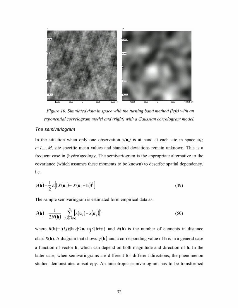
pairwise correlations. In practice, a manual "try and error" fitting is applied, relying

totally on visual criteria. Data are usually too sparse to allow identifying the true structure

of the studied spatial process. The importance of the choice of theoretical covariance

model is revealed only when using the identified covariance structure for simulation of

spatial fields. Fig. 10 shows the results of simulations with equal spatial integral scales of

the model but with the two extremes of smoothness, exponential and Gaussian,

respectively. The difference is striking and underlines the importance of the choice of

theoretical correlation to be used for simulations.

32

Figure 10. Simulated data in space with the turning band method (left) with an

exponential correlogram model and (right) with a Gaussian correlogram model.

The semivariogram

In the situation when only one observation x(ui) is at hand at each site in space ui,;

i=1,...,M, site specific mean values and standard deviations remain unknown. This is a

frequent case in (hydro)geology. The semivariogram is the appropriate alternative to the

covariance (which assumes these moments to be known) to describe spatial dependency,

i.e.

( ) ( ) ( )( )[ ]2ii2

1 huuh +−= XXEγ (49)

The sample semivariogram is estimated form empirical data as:

( ) ( ) ( ) ( )[ ]( ) ( )∑∈

−=N

Rjixx

N huu

hh

,

2ji2

1γ (50)

where R(h)=(i,j):|h-ε|≤|ui-uj|≤|h+ε| and N(h) is the number of elements in distance

class R(h). A diagram that shows ( )hγ and a corresponding value of h is in a general case

a function of vector h, which can depend on both magnitude and direction of h. In the

latter case, when semivariograms are different for different directions, the phenomenon

studied demonstrates anisotropy. An anisotropic semivariogram has to be transformed

33

into an isotropic one in order to be used (Journel and Huijbregts, 1978). In the following,

isotropy will be assumed and, thus, distance can be handled as a scalar h.

It can be expected, that the difference [X(i)-X(i+h)] increases with the distance between

observations, h. Observations, situated in the vicinity of each other, can be expected to be

more alike than those far away. However, in practice γ(h) often approaches some positive

value C0, called the "nugget-effect", when h approaches zero. This value reveals a

discontinuity in the semivariogram in the vicinity of the origin of coordinates at the

distance that is shorter than the shortest distance between observation points. This

discontinuity is caused by variability in a scale smaller than the shortest distance and also

by observation errors.

The procedure of estimation of a theoretical model to an experimental variogram depends

on discrete empirical values at specified distances. It can involve a certain degree of

subjectivity. Procedures for automatic estimation are least square estimation (LSE),

maximum likelihood (ML) and Bayesian estimators (Smith, 2001). Such automatic

methods are becoming more frequent in hydrology but still subjective trial-and-error

fitting dominates. An experimental variogram is very sensitive to errors and uncertainties

in data (Gottschalk et al., 1995).

Similar to the premises that have been formulated for a theoretical correlation function,

the following conditions should be satisfied for a theoretical semivariogram (Christakos,

1984):

i) A semivariogram γ(h) should be a real, even and continuous function (possibly with the

exception of h=0) for which the following condition is valid for any h:

( ) ( )hh γγ =− (51)

ii) The value of this function should follow the following dependency when h approaches

infinity :

( )∞→= h

hhlim 02

γ (52)

34

iii) Variance of linear combinations of variables X(ui), i=1,...,M, in accordance with

eq.(1.9) must be positive, which is satisfied when -γ(h) is conditionally positively

definite, i.e.:

( )∑∑= =

>M

j

M

kkj h

1 10γλλ when ∑

=

=M

ji

10λ for all M. (53)

In this case it can be noted that there is no demand that γ(h) should have some upper

boundary as in the case of the correlation (covariance) function, which might be seen as

an advantage of using the semivariogram.

0 1 2 3 4 5 60

20

40

60

80

100

distance

"Sill"

"Nugget"

"Range"

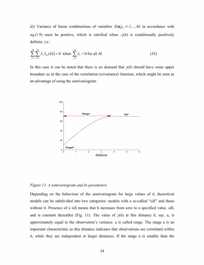
Figure 11. A semivariogram and its parameters.

Depending on the behaviour of the semivariogram for large values of h, theoretical

models can be subdivided into two categories: models with a so-called “sill” and those

without it. Presence of a sill means that h increases from zero to a specified value, sill,

and is constant thereafter (Fig. 11). The value of γ(h) at this distance h, say, a, is

approximately equal to the observation’s variance. a is called range. The range a is an

important characteristic as this distance indicates that observations are correlated within

it, while they are independent at larger distances. If the range a is smaller than the

35

shortest distance between observations, a pure nugget-effect is observed i.e. data are

independent. The phenomenon studied demonstrates in this case a completely random

pattern with respect to the distances between observation points available.

Below, five often used theoretical semivariograms are presented: a) linear; b) spherical;

c) Gaussian; d) exponential and e) fractal. The nugget-effect is denoted by C0, sill is

denoted by C0+C1 and range by a:

a)

0 1 2 3 4 5 60

20

40

60

80

100

distance

varia

nce

b)

0 1 2 3 4 5 60

20

40

60

80

100

distance

varia

nce

d)

0 1 2 3 4 5 60

20

40

60

80

100

distance

varia

nce

c)

0 1 2 3 4 5 60

20

40

60

80

100

distance

varia

nce

e)A=10

0 1 2 3 4 5 60

20

40

60

80

100

distance

varia

nce

B=0.5

B=1.0

B=1.5

Figure 12 Examples of theoretical semivariograms: a) linear, b) spherical, c) Gaussian,.

d) exponential, e) fractal.

a) Linear (Figure 12a)

( )( ) ahCCh

ahhBCh≥+=

<≤∗+=

10

0 0γγ

(54)

where B is the slope for 0≤h≤a.

b) Spherical (Figure 12b)

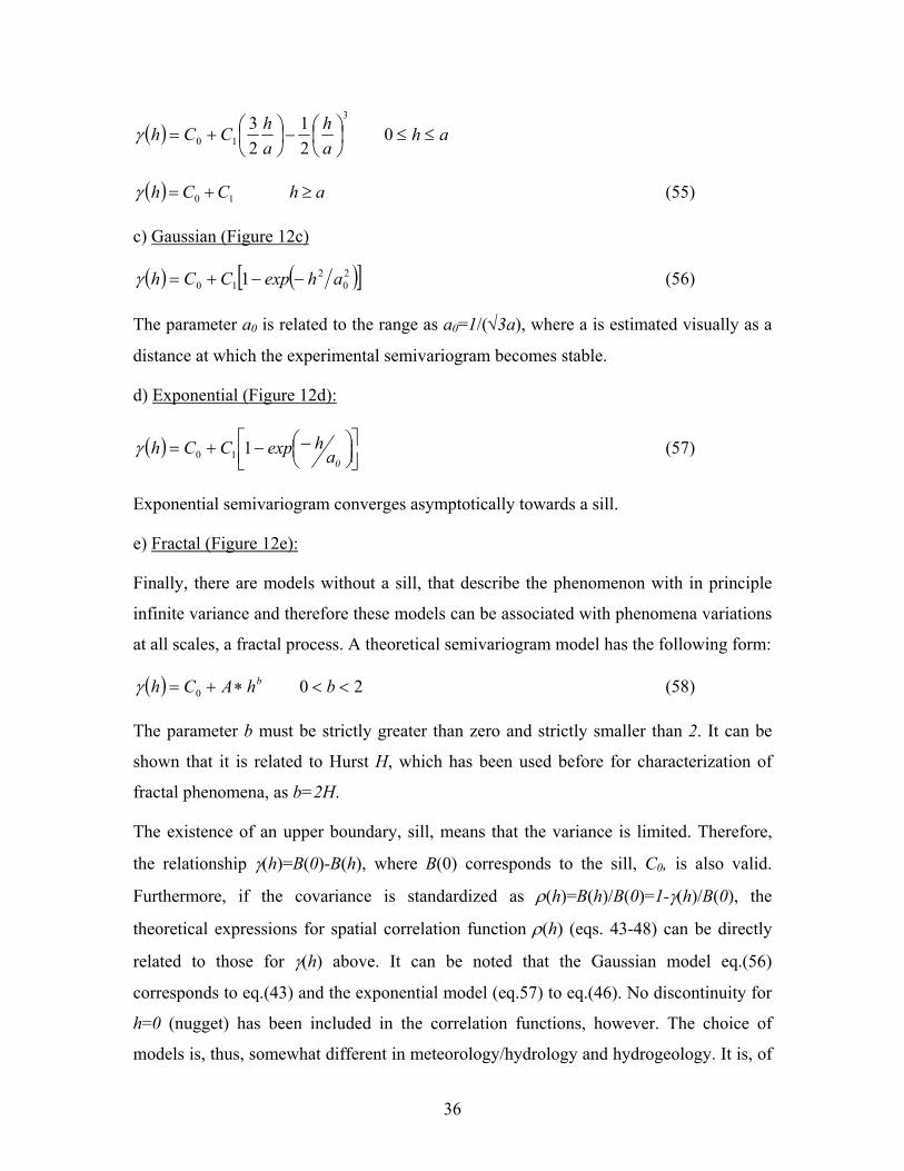
36

( ) ahah

ahCCh ≤≤

−

+= 0

21

23 3

10γ

( ) ahCCh ≥+= 10γ (55)

c) Gaussian (Figure 12c)

( ) ( )[ ]20

210 1 ahexpCCh −−+=γ (56)

The parameter a0 is related to the range as a0=1/(√3a), where a is estimated visually as a

distance at which the experimental semivariogram becomes stable.

d) Exponential (Figure 12d):

( )

−−+=

0ahexpCCh 110γ (57)

Exponential semivariogram converges asymptotically towards a sill.

e) Fractal (Figure 12e):

Finally, there are models without a sill, that describe the phenomenon with in principle

infinite variance and therefore these models can be associated with phenomena variations

at all scales, a fractal process. A theoretical semivariogram model has the following form:

( ) 200 <<∗+= bhACh bγ (58)

The parameter b must be strictly greater than zero and strictly smaller than 2. It can be

shown that it is related to Hurst H, which has been used before for characterization of

fractal phenomena, as b=2H.

The existence of an upper boundary, sill, means that the variance is limited. Therefore,

the relationship γ(h)=B(0)-B(h), where B(0) corresponds to the sill, C0, is also valid.

Furthermore, if the covariance is standardized as ρ(h)=B(h)/B(0)=1-γ(h)/B(0), the

theoretical expressions for spatial correlation function ρ(h) (eqs. 43-48) can be directly

related to those for γ(h) above. It can be noted that the Gaussian model eq.(56)

corresponds to eq.(43) and the exponential model (eq.57) to eq.(46). No discontinuity for

h=0 (nugget) has been included in the correlation functions, however. The choice of

models is, thus, somewhat different in meteorology/hydrology and hydrogeology. It is, of

37

course, possible to choose any of the semivariogram models referred to earlier and/or

correlation functions with or without a nugget. The only exception is the fractal model

eq.(58), which does not have a bounded variance.

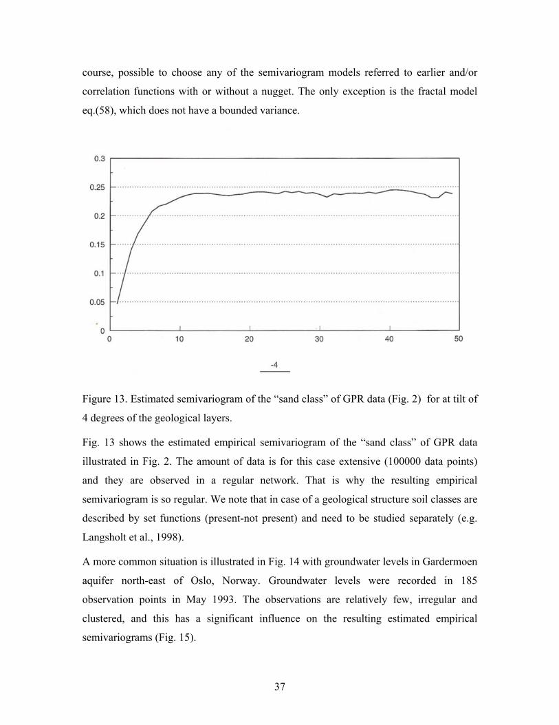
Figure 13. Estimated semivariogram of the “sand class” of GPR data (Fig. 2) for at tilt of

4 degrees of the geological layers.

Fig. 13 shows the estimated empirical semivariogram of the “sand class” of GPR data

illustrated in Fig. 2. The amount of data is for this case extensive (100000 data points)

and they are observed in a regular network. That is why the resulting empirical

semivariogram is so regular. We note that in case of a geological structure soil classes are

described by set functions (present-not present) and need to be studied separately (e.g.

Langsholt et al., 1998).

A more common situation is illustrated in Fig. 14 with groundwater levels in Gardermoen

aquifer north-east of Oslo, Norway. Groundwater levels were recorded in 185

observation points in May 1993. The observations are relatively few, irregular and

clustered, and this has a significant influence on the resulting estimated empirical

semivariograms (Fig. 15).

38

Figure 14. Location of 185 observation points of groundwater levels in the Gardermoen

area in May 1993 (from Engen, 1995).

The estimated global semivariogram from these data is presented in Fig. 15a. Fig. 15b

shows the four directional semivariograms (note the difference in scale for the variogram

between the two figures). Irregular and limited amount of data results in irregular

empirical semivariograms. It is an evidence of the uncertainty in specifying spatial

dependence in the same manner as the scatter of estimates of spatial correlation in Fig. 8.

39

Figure 15. Estimated global semivariogram (left) and four direction variograms (right) (from Engen,

1995).

3.4 Spatial-temporal random processes The most general case is a random process in time as well as in space. The observations

are thus not realisations of a random vector as in the previous case but rather a set of time

series for each site of observation. In the general case the joint time space dynamics of

the process under study needs to be considered in terms of two dimensional time-space

covariance functions. Common examples are the development of precipitation over an

area at a time scale of minutes or hours and runoff at an hourly time scale for a small

catchment. At larger time scales say a week, a month or a year in most hydrologic

situations there exists no dynamic link between the processes in space and time and they

can be treated separately by a covariance structure in space and another in time. The

methods that are developed below in section 4 of this chapter are well suited to handle

this latter situation. For the general case a dynamic spatial-temporal model needs to be

formulated. Models for precipitation may serve as examples (e.g. Northrop et al., 1999).

For simple linear hydrologic systems expressed in terms of an ordinary or partial

differential equation it is possible to directly derive a theoretical covariance function from

these equations (Gottschalk, 1977, 1978). Here only some simple examples of time-space

correlation functions are treated.

For the general formulation of a time-space process Vanmarcke (1988) distinguishes

between three important special types of two dimensional covariance functions, namely:

• the covariance structure is separable, i.e. ( ) ( ) ( )τρρστρσ hh 22 , = and an example

is: ( ) ( ) ( ) 22

21

22 exp, kkhh τστρσ −−=

• the correlation structure is isotropic, i.e. the covariance structure can be expressed

in terms of the “radial” covariance function where 22 τ+= hr :

( ) ( ) ( ) ( )τρσρσρσρσ ,,00, 2222 hrrrR ===

• the covariance structure is ellipsoidal, i.e. by appropriate scaling and rotation of

the coordinate axes random fields with ellipsoidal covariance structure can be

reduced to isotropic random fields.

40

Gandin and Kagan (1976) suggest a covariance model similar to the second type for use

in meteorology and climatology:

[ ] ( )( )τρστ += vhh 2,Cov (59)

where v is a velocity and h/v can be interpreted as a time of travel. Bass (1954) refers to a

similar expression for application in turbulence theory.

4 Karuhnen-Loève expansion

4.1 Introduction A technique of expanding a deterministic function f(t), defined on a finite interval [a,b],

into a series, based on some special deterministic orthogonal function (e.g. a Fourier

series), is well-known from mathematics. The problem can be generalized also to two

dimensions where function f(u) is defined for an area Ω (e.g. two-dimensional Fourier

series). In a similar manner a random function can be expanded in terms of random

variables and deterministic orthogonal functions. The “proper orthogonal decomposition

theorem” (Loève, 1945) states: “A random function X(t) continuous in quadratic mean on

a closed interval has on this interval an orthogonal decomposition:

( )∑= ttX nnn ψξλ)( (60)

with

[ ] ,mnnmE δξξ = (61)

( ) ( ) mnnm dttt δψψ =∫ (62)

if, and only if, the 2nλ are the proper values (eigenvalues) and the ( )tnψ are the

orthonormalised proper functions (eigenfunctions) of its covariance. Then the series

converges in quadratic mean uniformly on I”.

The eigenfunctions, which as noted from the above theorem are the eigenfunctions of the

covariance, are thus determined from the following equation (a Fredholm’s integral

equation of the first type)

41

( ) ( ) ( )ttdtttB nnn ψλψ 2, =′′′∫ (63)

Furthermore the covariance can be written as a series expansion

( ) ( )[ ] ( ) ( ) ( )∑ ′=′=′ ttttBtXtXCov nnn ψψλ 2, (64)

which for the variance reduces to the simple expression

( )[ ] ( ) ∑== 2,Var nttBtX λ (65)

The nξ s are random variables and are derived from the relation

( ) ( )∫= dtttX nnn ψξλ (66)

The covariance between the random function X(t) and nξ is

( )[ ] ( )ttXCov nnn ψλξ = (67)

The representation eq. (60) of a random function is widely used under the name

“Karhunen – Loève expansion”. It appears to have been introduced independently by a

number of scientists (see Lumley, 1970): Kosambi (1943), Loève (1945), Karhunen

(1946), Pougachev (1953) and Obukhov (1954). In case of normally distributed data the

statistical orthogonality eq. (61) is equivalent to independence and the projection eq. (66)

is equivalent to conditioning. Karhunen – Loève expansion is used for analysing data in

terms of a “spectral” representation, for reconstruction and simulation of data. It might

also be an effective tool for dimensionality reduction of large data sets to eliminate

redundant information.

5.2 Harmonic (spectral) analysis

In physics, the most important orthogonal decomposition is the harmonic one, for,

loosely speaking, it yields “amplitudes”, and hence “energies”, corresponding to various

parts of the “spectrum” of the random function. Following Loève’s strict formulation the

random function has an imaginary as well as a real part. A more physical approach avoids

complex number algebra (Vanmarcke, 1988). In this latter case the stationary random

function X(t) is expressed as a sum of its mean m=c0/2 and 2K sinusoids with positive and

negative frequencies fk=±kf1, random amplitudes ck and phase angles θk, k=1,...,K.

42

( ) ( )∑−=

++=K

Kkkkk tfcctX θπ2cos02

1 (68)

All random amplitudes and phase angles are mutually independent random variables and

the phase angles are uniformly distributed over [0,2π]. Every single term in the sum has a

mean zero and the variance [ ].2212

kcEk =σ , and the total variance

( )[ ] [ ]∑= 221Var kcEtX (69)

Equations (68) and (69) have there direct parallels to equations (60) and (65) above.

Generalizing to a continuous spectrum for a homogeneous process, i.e. with

B(t,t’)=B(|t-t’|) we derive the two-sided spectral function eq. (12). It can be rewritten with

the help of known trigonometric relationships and taking into consideration that S(f) is an

even function, as:

( ) ( )∫∞

∞−

−= '' '22 dtettBefS tfitfi ππ (70)

This expression can be compared with eq.(63). Similar results can be obtained if [a,b] is

finite, as long as the spectrum S(f) is a rational function. Analytical expressions for this

case can be found in Davenport and Root (1958) and Fortus (1973).

5.3 Wavelet analysis In the Fourier series representation the orthonormal base function ( )tnψ is generated by

dilation of a single function ( ) itet =ψ , i.e. ( ) ( )nttn ψψ = . For any integer n with large

absolute value, the wave has high frequency, and for n with small absolute value, the

wave has low frequency. So every function is composed of waves with different

frequencies. The sinusoidal function is defined on one period of 2π and the condition for

the existence of a series expansion is that the random function is absolute integrable over

this period.

( ) ∞<∫ dttX 22

0

π (71)

In case of wavelets the point of departure is also an orthogonal decomposition in

accordance with eq. (60) (Chui, 1992). The difference first of all lays in the fact the

43

random function is defined on the real line and that the random function thus satisfies the

condition

( ) ∞<∫∞

∞−dttX 2 (72)

The two function spaces are quite different since, in particular, the local average of every

function must decay to zero at ∞± and the sinusoidal (wave)functions do not satisfy this

condition. Waves that can satisfy this condition should decay to zero at ∞± , and for all

practical purposes the decay should be fast. Small waves or “wavelets” are thus

appropriate. It is preferred to have one single generating function, like in Fourier series

(mother wavelet or analyzing wavelet ( )tψ ). But if the wavelet has a very fast decay,

how, can it cover the whole real line? The answer is to allow shifts along the real line.

The power of two is used for frequency partitioning

( )ktj −2ψ (73)

It is obtained from a single wavelet function by binary dilation (i.e. dilation by 2j) and

dyadic translation (of k/2j). Normalisation results in:

( ) ( )ktt jjkj −= 22 2

, ψψ (74)

The normalising equation corresponding to eq. (62) has the form

( ) ( ) kmjlmlkj dttt δδψψ =∫∞

∞− ,, (75)

The series expansion is written:

( )∑ ∑∞

−∞=

∞

−∞=

=j k

kjkj ttX ,,)( ψβ (76)

The coefficients in the series expansion are determined from

( ) ( )∫= dtttX kjkj ,, ψβ (77)

A simple example is the Haar function

44

( )

<≤−

<≤

=

else011

01

21

21

tt

tHψ (78)

Similar to the harmonic analysis we can turn over to a continuous representation and

define a wavelet transform as (Chui, 1992):

( ) ( )∫∞

∞−

−

= dts

ts

txsW τψτ *1, (79)

where ψ*(t) is the complex conjugate of ψ (t). The inverse transform of eq. (79) for

reconstruction of x(t) is written down as:

( ) ( )∫ ∫∞

∞−

∞

∞−

−

= dtds

ts

sWC

tX ττψτψ

21,1 (80)

where Cψ is a constant of admissibility, which depends on the wavelet used and needs to

satisfy the condition:

( )∞<= ∫

∞

∞−

ωωωψ

ψ dC2ˆ

(81)

( ( )ωψ is the Fourier transform of ψ (t)).

Basic works introducing wavelets are those by Grossman and Morlet (1984) and Meyer

(1988). Wavelet decomposition has found many applications in for instance image

processing and fluid dynamics and turbulence. Wavelets also provide a convenient tool

for studying scaling characteristics of a random process (Mallat, 1989; Wornell, 1990;

Kumar and Foufula-Georgiou, 1993). A simple example from Feng (2002) illustrates the

application to hydrologic data (Fig. 15). In this case a quadratic spline function is used as

mother wavelet to be able to reconstruct and simulate observed periodic hydrological

time series.

45

Figure 15. Illustration of traditional wavelet decomposition and reconstruction: upper

graph shows measured time series with five main periods; middle graphs decomposed

wavelet series ( )tnψ ; and lower graph reconstructed series (from Feng, 2002).

5.4 Principal Component Analysis (pca)

The basic matrix equation for the principal component analysis of a random function is

expressed as

ΛΨ=ΨXB (82)

where in the general case BX is a covariance matrix, Ψ a coefficient matrix of

eigenvectors and Λ a diagonal matrix of eigenvalues. Each M by M symmetrical

positively definite covariance matrix BX has a set of M positive eigenvalues. Furthermore,

there exists a linear transformation Z=ΨTX of the original observation matrix X which

46

has a diagonal covariance matrix BZ. ΨT is an M by M coefficient matrix representing the

eigenvectors of BX. The variables Z are named Principal Components. The observation

matrix X can now be expressed as a linear combination of the principal components:

ZX Ψ= (83)

The coefficient matrix Ψ is orthogonal, i.e. ΨΨT=I. The principal components Z have the

following covariance matrix:

Λ=ΨΨ== XT

Z1 BZZB T

n (84)

where BX is, as before, the covariance matrix of X, BX=(1/n)XXT and Λ is the diagonal

matrix of eigenvalues λ2j, j=1,...,M. If eq. (83) is written as a sum:

ntMjzzxM

kktkjk

M

kktjkjt ,...,1;,...,1;

11

==′== ∑∑==

λψψ (85)

where z’k is the normalised values of zk with respect to its variance λk . Parallels to eq.

(60) can be seen clearly by a simple exchange of symbols. From eq.(84) we have:

Mkjzzn

zzn

n

tjkktjt

n

tjkkktjt ,,1,1;1

11

2K==′′= ∑∑

==

δδλ (86)

and using the condition of orthogonality of the coefficient matrix Ψ we get:

∑=

==M

ljklkjl Mkj

M 1,,1,;1

Kδψψ (87)

Finally, multiplying eq.(84) by Ψ from the left yields:

∑=

==M

ljkjlkjk MjB

1,,1, Kψλψ (88)

Also here there are parallels to eqs. (61), (62) and (63), respectively, if a symbol change

is done.

The method of pca representation is usually carried out in terms of the solution of the

matrix equation eq. (82) of very general applicability. Principal component analysis

(factor analysis) has its root in psychometrics. The classical work is the one by Hotelling

47

(1933). The generality of the method might be a strength for many applications, but with

caution. Hydrological time series data are as a rule collected at regular time intervals.

For this case we can apply the matrix equation as a simple approximation of the more

general eq. (63). In the case of application to spatial data in meteorology, as pointed out

by Buell (1971), there are very strong geometrical elements (in the general case the

covariance matrix represents covariances between irregularly spaced observation points)

that can be advantageous, but which are missing in the matrix formulation. Hydrological

applications have as a rule the same strong geometrical elements and BX is usually the

covariance matrix (eq.33) with elements Bij = E[(xi-mi)(xj-mj)], i,j=1,...M, covariances

between values xi measured at point ui and xj measured at point uj.

It is found appropriate to differ between situations when geometrical aspects of the

problem are strong and when they are not. In the latter case the pca matrix formulation

eq. (82) is appropriate. In the other case the point of departure is eq. (63) and for discrete

data a numerical solution of this equation should be developed. The name for this

situation that will be used here is empirical orthogonal functions (eof).

5.6 Empirical orthogonal functions (eof).

The notion of empirical orthogonal functions, was first introduced in the classical work

by Lorenz (1956). Other earlier applications of this technique in meteorology are those by

Obukhov (1960) and Holmström (1963) (without using the name “eof”). Already Lorenz

mentions the parallel in the problem with that of factor analysis (principal component

analysis) used by psychologists quoting the classical work by Hotelling (1933). The point

of departure for the development of this technique for Lorenz was dimensionality

reduction, i.e. getting rid of the large amount of redundant information contained in

meteorological data. In psychology, on the other hand, the central point was to interpret

psychological tests into observed behaviour of their patients. Today both approaches are

used in meteorology and climatology as well as in hydrology and a difference can be

traced in the interpretation of the empirical functions – are those only mathematical

constructions or can they be interpreted in some process oriented way. In the latter case

this has led forward to the use of rotations of the principal components yielding

possibilities for a better interpretation of results (see Richman (1986) and Jolliffe

48

(1990,1993) for an overview). Long unfruitful discussions about the possible distinction

between pca and eof can be found in the climatological literature. One such distinction

should be related to how the normalisation is performed.

The point of departure in the works by Lorenz and Holmström is a random process X(u,t)

that develops in space u=(u1,u2) over a certain domain in space Ω and time t. Eq. (63) is

for this case generalised to a process in space:

( ) ( ) ( )uuuuu nnn dB ψλψ 2, =′′′∫Ω

(89)

It is important to emphasize that this integral equation formulation is the appropriate one

for problems like in meteorology and hydrology dealing with a random function X on a

continuum in space. The geometrical relations involving the domain of integration and

the relations between the points ui, i=1,...,M are completely ignored in the matrix

formulation. The fact that function values are obtained from measurements at discrete

points (perhaps sparsely located) is a practical limitation to the numerical solution of the

problem (e.g. Obled and Creutin, 1986).

X(u,t) is expanded into double orthogonal series of the form:

( ) ( ) ( )∑=n

nn tztX uu ψ, (90)

where eigenfunctions ψj(u) and ψk(u) as before are analytically orthogonal:

( ) ( )∫ ∫Ω

= kjjk d δψψ uuu (91)

i.e. ψk(u) can be regarded as a deterministic function. It is determined by numerical

solution of eq. (89). The functions ψk(u) depend both on the covariance function and the

area Ω.

zj(t) and zk(t), on the other hand, are statistically orthogonal or uncorrelated:

( ) ( )[ ] 2kkjjk tztzE λδ= (92)

where δkj is Kronecker's delta and λk2 is the eigenvalue as before.

The function zk(t) is obtained as:

49

( ) ( ) ( )∫ ∫Ω

= uuu dtXtz kk ψ, (93)

i.e. by means of projection of the realization at time t on the k-th eigenfunction.

For a given analytical expression for the autocorrelation function, eigenfunctions

corresponding to it can be found. Fortus (1975) and Braud (1990) show an analytical

solution for the case when Ω is a circle. B(u,v) can be written as a series expansion:

( ) ( ) ( )∑=n

nnnB vuvu ψψλ 2, (94)

in correspondence with eq. (64). The expansion eq.(90) can be truncated till, say, N terms

as:

( ) ( ) ( )∑=

=N

nnnN tztX

1,ˆ uu ψ (95)

which minimizes the variance in the estimation error of X by NX :

( ) ( ) uuu dtXtXE N

−∫ ∫

Ω

2,ˆ, (96)

and which obtains the value ∑∞

+= 1

2

Nnkλ . In case of high redundancy in the data the

expansion eq. (95) converges rapidly which indicates a possibility of truncating the series

expansion after rather few terms. This is the idea behind the use of eof for dimensionality

reduction. The functions zk(t), often called amplitude functions, represent time series that

are not linked to any specific points of the domain Ω. On the other hand they can be used

to construct X(uk,t) for a point uk if the functions Ψn(uk), n=1,...,N are known at this point.

Fig. 16 illustrates the principle where the eof method is applied to monthly runoff data

from the Rhône basin in France. Amplitude functions are shown as well the results of

prediction of the runoff pattern for independent stations to the right (Sauquet et al., 2000).

Fig. 3 in the introduction of this chapter shows a prediction of the monthly flow patterns

for the whole river system.

50

51

Figure 16. Example of spatial interpolation of monthly runoff patterns for the Rhone basin in France (upper map). The first six amplitude functions are shown to the left and the result of prediction of the runoff pattern for independent stations to the right (Sauquet et al., 2000).

Concluding remarks In the introductory part of this chapter it was adopted to use a partial characterization of

the random process under study in accordance with three different schemes:

iv) Characterization by distribution function (one dimensional),

v) Second moment characterization, and

vi) Karhunen-Loève expansion i.e. a series representation in terms of random

variables and deterministic functions of a random process.

This should not be understood so that one replaces the other. On the contrary these three

schemes for partial characterization complement each other. All methods of analysing

variability developed in this chapter are applied in practice without consideration of the

parent distribution of the data. On the other hand all these methods have a strong

theoretical base if normality can be assumed. For instance, as already noted normally

distributed data weak homogeneity equals strict homogeneity. For normally distributed

data statistical orthogonality is equivalent to independence and a projection onto a system

of orthogonal axes is equivalent to conditioning. Furthermore the assumption of

normality opens up for related statistical tests. Analyzing the distribution function of the

data is therefore a logical first step (after “looking at data”). If the data are far from

normally distributed it might be worthwhile to utilise a transformation to normal. The

following transformations to normality are often used in hydrology: i) ln(x) in case of

lognormally distributed data; ii) The cube root ( )31

xx (Wilson & Hilferty, 1931)

transformation in case of gamma distributed data; and iii) the more general power

transformation ( )[ ] hcx h 1−+ , where h and c are parameters (Box and Cox, 1964).

The characterization by second moments allows establishing the structure of the data in

space and time and its scale of variability. It also gives the possibility of testing basic

hypothesis of homogeneity and stationarity. By means of normalization and

standardization data can be transformed into new data sets owing these properties. The

52

characterization by series representation in its turn assumes homogeneity with respect to

the variance-covariance function. It is as such a tool for analyzing spatial-temporal

variability relative to the first and second order moments in terms of new sets of common

orthogonal random functions.

The conclusions is thus that the approaches developed here form logical steps in a

sequential analysis of variability: i) looking at data, exploring data; ii) analyzing the

distribution of data; iii) analyzing first and second order moments; iv) analyzing data by

means of series expansion.

References Bass, J (1954) Space and time correlations in a turbulent fluid, Part I. Univ. of California

Press, Berkely and Los Angeles, 83p. Beran, J. (1994) Statistics for long memory processes. Vol. 61 of Monographs on

Statistical and Applied Probability, Chapman and Hall, New York. Box, G.E.P. and Cox, D.R. (1964) An analysis of transformations. J.R. Statist. Soc. B

26:211. Box, G.E.P. and Jenkins, G.M. (1970) Time series analysis, forecasting and control.

Holden Day, San Fransisco. Braud, I. (1990) Etude méthodologique de l’Analyse en Composantes Principales de

processes bidiminsionelles. Doctorat INPG, Grenoble. Buell, E.C. (1971) Integral equation representation for factor analysis. J.Atmos.Sci. 28:

1502-1505. Chow, Ven-te (1954) The log-probability law and its engineering application.

Proceedings ASCE Vol 80, separate. Christakos, G. (1984) On the problem of permissible covariance and variogram models.

Wat.Resour.Res. 20(2): 251-265. Chui, C.K. (1992) An introduction to wavelet. Academic Press, Boston. Davenport, W.B. and Root, W.L. (1958) An Introduction to the Theory of Random

Signal and Noise. McGraw-Hill. Engen, T. (1995) Stokastisk interpolasjon av grunnvannspeilet i israndsdeltaet på

Gardermoen. Hovedfagsoppgave i hydrologi. Institutt for Geofysikk, Universitet i Oslo.

Feng, G. (2002) A method for simulation of periodic hydrological time series using wavelet transform. In. Bolgov, V., Gottschalk, L., Krasovskaia, I. and Moore, R.J. (eds.) “Hydrological Models for Environmental Management”, NATO Science series, 2. Environmental Security – Vol. 79, Kluwer Academic Publishers, Dordrecht.

Fennessey, N.M. and Vogel, R.M. (1990) Regional flow duration curves for ungauged sites in Massachusetts. Journal of Water Resources Planning and Management 116(4):530-549.

Fortus, M.I. (1973) Statistically orthogonal functions of a finite interval of a stochastic process (in Russian). Fizika Atmosfery I Okeana IX(1).

53

Fortus, M.I. (1975) Statistically orthogonal functions of stochastic fields defined for a finate area (in Russian). Fizika Atmosfery I Okeana XI(11).

Foster, A. (1923) Theoretical frequency curves. Proceedings ASCE. Foster, A. (1924) Theoretical frequency curves and their application to engineering

problems. Transactions ASCE Vol. (87). Foster, A. (1933) Duration curves. Transactions ASCE 99 :1213-1267. Gandin, L.S. and Kagan, P.L. (1976) Statistical methods for interpretation of

meteorological observations (in Russian). Gidrometeoizdat, Leningrad. Gelfand, I.M. and Vilenkin, N.Ya. (1964) Generalazed functions. Vol. 4: Applications of

Harmonic Analysis. Academic Press, New York. Gosh, B. (1951) Random distances within a rectangle and between two rectangles. Bull.

Calcutta Math. Soc. 43. Gottschalk, L. (1977) Correlation structure and time scale of simple hydrological

systems. Nordic Hydrology 8:129-140. Gottschalk, L. (1978) Spatial correlation of hydrologic and physiographic elements.

Nordic Hydrology 9:267-276. Gottschalk, L. Krasovskaia, I. and Kundzewicz, Z.W. (1995) Detecting outliers in flood

data with geostatistical methods. In: Z.W.Kundzewicz (ed.) “New Uncertainty Concepts in Hydrology and Water resources”, Cambridge Univ. Press: 206-214, 1995.

Grossman, A. and Morlet, J. (1984) Decomposition of Hardy functions into square integrable wavelets of constant shape. SIAM Journal of Math. Anal. 15(4):723-736.

Handcock, M.S and Stein, M.L. Stein (1993) A Bayesian analysis of kriging. Technometrics 35(4):403-410.

Hansen, E. (1971) Analyse af hydrologiske tidsserier. (in Danish) Polyteknisk forlag, København.

Hazen, A. (1917) The storage to be provided in impounding reservoirs for municipal water supply. Transactions ASCE.

Holmes, M.G.R., Young, A.R., Gustard, A. and Grew, R. (2002) A region influence approach to predicting flow duration curves within ungauged basins. Hydrology and Earth System Sciences 6(4):721-731.

Holmström, I. (1963) On a method for parametric representation of the state of the atmosphere. Tellus 15(2):127-149.

Holmström, I. (1970) Analysis of time series by means of empirical orthogonal functions. Tellus 22:638-647.

Hotelling, H. (1933) Analysis of a complex of statistical variables into principal components. J. Educ. Psychol. 24:417-441,498-520.

Hurst, H.E. (1951) Long-term storage capacity of reservoirs. Trans. ASCE, Vol.116, 770-799.

Jolliffe, I.T. (1990) Principal component analysis: A beginner’s guide – I. Introducation and application. Weather 45:375-382.

Jolliffe, I.T. (1993) Principal component analysis: A beginner’s guide – II. Pitfalls, myths and extensions. Weather 48:246-252.

Journel, A. and Huijbregts, Ch.J. (1978) Mining Geostatistics. Academic Press, New York.

54

Karhunen, K. (1946) Zur spektraltheorie stochastic prozesse. Annales Academiae Scientarium Fennicae Series A I. Mathematica-Physica 34, Helsinki.

Kendall, M., Stuart, A. and Ord, J.K. (1987) Kendall’s Advanced Theory of Statistics (Ch. 10 Standard Errors). Charles Griffin, London.

Khinchine, A.I. (1949) Mathematical foundations of statistical mechanics. Dover, New York.

Kolmogorov, (1941) The local turbulence structure of an incompressible viscous liquids for very big Reynolds numbers (in Russian). Doklady Acad. Nauk SSSR, 30(4):299-303.

Kosambi, D.D. (1943) Statistics in function space. J. Indian Math. Soc. 7:76-88. Koutssoyannis, D. (2002) The Hurst phenomenon and fractional Gaussian noise made

easy. Hydrological Sciences Journal 47(4):573-595. Koutssoyannis, D. (2003) Climate change, the Hurst phenomenon, and hydrological

statistics. Hydrological Sciences Journal 47(4):573-595. Krasovskaia, I. and Gottschalk,L. (1992) Stability of River Flow Regimes. Nordic

Hydrology, 23:137-154. Krasovskaia,I. (1996) Sensitivity of the stability of river flow regimes to small

fluctuations in temperature. Hydr.Sci.J., 41(2), 251-264 Krasovskaia, I., Gottschalk, L. & Kundzewicz, Z.W. (1999) Dimensionality of

Scandinavian river flow regimes. Hydrologica Science Journal 45(5):705-723. Kritskij, S.N. and Menkel, M.F. (1946) On models for studies of random variations in

river runoff (in Russian). In “runoff and hydrological calculations”, Ser. IV, Vyp. 29, Gidrometeoizdat, Leningrad.

Kumar, P. and Foufoula-Georgiou, E. (1993) A new look at rainfall fluctuations and scaling properties of spatial rainfall using orthogonal wavelets. Journal off Allied Meteorology 32:209-222.

Langsholt, E., Kitteröd, N-O. and Gottschalk, L. (1998) Development of 3-dimensional hydrostratigraphical models based on soft and hard data. Ground Water 36(1):104-111.

Loève, M. (1945) Fonctions aleatoire de second ordre. Compt Rend. Acad. Sci. (Paris) 220.

Lorenz, E.N. (1956) Empirical orthogonal functions and statistical weather prediction. MIT Department of Meterology, Statistical forecasting project, Scientific report no 1, Cambridge, Massachusetts.

Lumley, J.L.(1970) Stochastic tools in turbulence. Academic Press, New York and London.

Mallat, S.G. (1989) A theory for multiresolution signal decomposition : the wavelet representation. IEEE Tansactions on Pattern Analysis and Machine Intelligence 11(7): 674-693.

Matheron, G. (1965) Les variables régionalisées et leur estimation. Masson, Paris. Mandelbrot, B.B. and Van Ness, R., (1968) Fractional Brownian Motions, fractional

noises and applications. SIAM Review,.10( 4): 422-437. Mandelbrot, B.B. and Wallis, J.R. (1968) Noah, Joseph and operational hydrology. Water

Resour.Res., 4(5):

55

Mandelbrot, B.B. and Wallis, J.R. (1969a.) Computer experiments with fractional gaussian noises. Part 1: Averages and variances. Part 2: Rescaled ranges and spectra. Part 3: Mathematical appendix. Water Resour.Res., 5( 1)

Mandelbrot, B.B. and Wallis, J.R. (1969b) Some long run properties of geophysical records. Water Resour.Res., 5(1):

Meyer, Y. (1988) Ondelettes et Operateurs. Hermann. Mimikou, M. and Kaemak, S. (1985) Regionalization of flow duration characteristics.

Journal of Hydrology 82:77-91. Mosley, M.P. and McKerchar, A.I. (1992) Ch. 8 Streamflow in Maidment D.R. (ed.)

Handbook of Hydrology, MCGraw-Hill, N.Y. (p 8.27) National Research Council (1991) Opportunities in the hydrologic sciences. National

Academy Press, Washington D.C. Northrop, P.J., Chandler, R.E., Isham, V.S., Onof, C. and Wheater, H.S. (1999) Spatial-

temporal stochastic rainfall modelling for hydrological design. IAHS publication no. 255:225-235.

Obled, C. and Creutin, J.D. (1986) Some developments in the use of Empirical Orthogonal Functions for mapping meteorological fields. J.Appl.Meteorol. 25(9): 1189-1204.

Obukhov, A.M. (1954) Statisticheskii opisanie nepereryvnikh polej (Statistical description of continous fields). Akademii Nauk SSSR, Trudy Geofizicheskogo instituta no 24(151):3-42.

Obukhov, A.M. (1960) O statisticheski ortogonalnykh pazlozheniyakh empericheskyikh funktsii (On statistical orthogonal expansions of empirical functions). Izvestija Akademii Nauk SSSR, Ser. Geofizicheskaja 3: 432-439.

Pougachev, V.S. (1953) Obschaya teoriya korrelatsii cluchainykh funktsii (A general theory of korrelation of random functions). Izvestija Akademii Nauk SSSR, Ser. matematicheskaja 17: 401-420.

Richman, M.R. (1986) Rotation of principal components. Journal of Climatology 6:293-335.

Sauquet, E., Krasovskaia, I. and Leblois, E. (2000) Mapping mean monthly runoff patterns using EOF analysis. Hydrology and Earth System Science 4(1):79-73.

Sauquet, E. and Leblois, E. (2001) Mapping runoff within the GEWEX-Rhone project. La Houille Blanche, 2001(6-7): 120-129.

Searcy, J.K. (1959) Flow duration curves. U.S. Geological Survey Water Supply Paper 1542-A, 33p.

Singh, R.D., Mishra, S.K. and Chowdhary, H. (2001) Regional flow-duration models for large number of ungauged Himalayan catchment for planning microhydro projects. Journal of Hydrologic Engineering 6(4):310-316.

Skaugen, T. Personal communication 1993. Smith, R.L. Environmental Statistics. Dep. of Statistics, University of North Carolina.

Web reference: /www.stat.unc.edu/postscript/rs/envnotes.ps, July 2001. Sokolovksij, D.L. (1930) Application of distribution curves to determine probability of

fluctuations in annual runoff for rivers in the European part of USSR (in Russian). Gostechizdat, Leningrad.

Tukey, J.W. (1977) Exploratory Data Analysis, Addison Wesley, Reading, Mass.

56

Vanmarcke, E. (1988) Random fields: Analysis and Synthesis, MIT Press Cambridge Mass. Third printing.

Vogel, R.M. and Fennessey, N.M. (1994) Flow duration curves I: New interpretation and confidence intervals. Journal of Water Resources Planning and Management 120(4):485-504.

Vogel, R.M. and Fennessey, N.M. (1995) Flow duration curves II: Application in water resources planning. Water Resources Bulletin 31(6):1029-1039.

Wiener, H. (1930) Generalized harmonic analysis. Acta Math. 55:117-258. Wiener, H. (1949) Extrapolation, interpolation and smoothing of stationary time series.

MIT Press, Cambridge, Mass. Wilson, E.B. and Hilferty, M.M. (1931) The distribution of chi-square. Proc. Nat. Acad.

Sci. USA 17:684. Wornell, G.W. (1990) A Karhunen-Loève-like expansion for 1/f processes via wavelets.

IEEE Tansactions on Information Theory 36(4):859-861. Yevjevich, V. (1972) Stochastic processes in hydrology. Water Resources Publications,

Forth Collins, Colorado. Yu, P.-S. and Yang, T.-C. (1996) Synthetic regional flow duration curve for southern

Taiwan. Hydrological Processes 10:373-391.