Large Panel Data Models with Cross-SectionalDependence: A Surevey

Hashem PesaranUniversity of Southern California, CAFE, USA, and Trinity

College, Cambridge, UK

A Course on Panel Data Models, University of Cambridge, 29May 2013

Introduction

I Early panel data literature assumed cross sectionallyindependent errors and slope homogeneity; and heterogeneityacross units was modelled by using unit-specic interceptsonly, treated as xed or random.

I Cross-sectional error dependence was only considered inspatial models, but not in standard panels. However, with anincreasing availability of data (across countries, regions, orindustries), panel literature moved from predominantly micropanels, where the cross section dimension (N) is large and thetime series dimension (T ) is small, to models with both Nand T large, and it has been recognized that, even afterconditioning on unit-specic regressors, individual units, ingeneral, need not be cross-sectionally independent.

I Ignoring error cross-sectional dependence can have seriousconsequences, and the presence of some form ofcross-sectional correlation of errors in panel data applicationsin economics is likely to be the rule rather than the exception.Cross correlations of errors could be due to omitted commone¤ects, spatial e¤ects, or could arise as a result of interactionswithin socioeconomic networks.

I Conventional panel estimators such as xed or random e¤ectscan result in misleading inference and even inconsistentestimators, depending on the extent of cross-sectionaldependence and on whether the source generating thecross-sectional dependence (such as an unobserved commonshock) is correlated with regressors.

I The problem of testing for the extent of cross-sectionalcorrelation of panel residuals and modelling the cross-sectionaldependence of errors are therefore important issues.

Outline

I Types of cross-sectional dependenceI Modeling cross-sectional dependence by a multi-factor errorstructure

I Estimation and inference on large panels with strictlyexogenous regressors and a factor error structure

I Estimation and inference on large dynamic panel data modelswith a factor error structure

I Tests of error cross-sectional dependence

Types of cross-sectional (CS) dependenceI Let fxit , i 2 N, t 2 Zg be a double index process dened ona suitable probability space and assume:

E (xt ) = 0, Var (xt ) = Σx ,

where xt = (x1t , x2t , ..., xNt )0 and the elements of Σx , denoted

as σx ,ij for i , j = 1, 2, ...,N, are uniformly bounded in N,namely jσx ,ij j < K .

I These assumptions could be relaxed, by consideringconditional expectations and variances, nonzero time-varyingmeans, and time-varying variances.

I Various summary measures of the matrix Σx have beenconsidered in the literature.

I The largest eigenvalue of Σx , denoted as λ1 (Σx ), hasreceived a great deal of attention in the literature, butλ1 (Σx ) is di¢ cult to estimate when the cross sectiondimension, N, is large compared to the time dimension, T .

I Chudik, Pesaran and Tosetti (2011) summarize the extent ofCS correlations based on the behavior of CS averages. Letxwt = ∑N

i=1 wixit , where the weights w = (w1,w2, ...,wN )0

satisfy the following granularityconditions:

kwk =pw0w = O

N1/2

, and

wikwk = O

N1/2

uniformly in i 2 N.

I fxitg is cross-sectionally weakly dependent (CWD) if for anysequence of granular weights w, we have

limN!∞

Var (xwt ) = 0.

Otherwise, fxitg is cross-sectionally strongly dependent(CSD).

I Bailey, Kapetanios and Pesaran (2012) characterize thepattern of cross-sectional dependence further. Let wi = N1,for all i , and consider

Var (xt ) = Var

1N

N

∑i=1xit

!=

1N2

N

∑i=1

σx ,ii +1N2

N

∑i=1

N

∑j=1,j 6=i

σx ,ij| z κx ,N

,

where jσx ,ij j < K and therefore 0 Var (Nxt ) < KN2.I The extent of cross-sectional dependence relates directly tothe term, κN , and Bailey et al. parametrize this term by anexponent of cross-sectional dependence α 2 [0, 1] thatsatises

limN!∞

N22ακx ,N = K for some constant 0 < K < ∞.

Spatial examples

I Leading examples of a cross sectionally dependent processesare factor models or spatial models.

I Spatial models of the error vector ut = (u1t , u2t , ..., uNt )0 can

be written asut = Rεt , εt (0, IN )

I For instance, R = (IN ρW)1 1/2, in the rst order spatialautoregressive model ut = ρWut +1/2εt , where is adiagional matrix. It is easy to see that ut is CWD when rowand column matrix norms of R are both bounded.

Modelling cross-sectional dependence by a factor errorstructure

I Consider the m factor model for fzitg

zit = γi1f1t + γi2f2t + ...+ γim fmt + eit , i = 1, 2, ...,N,

or, in matrix notations

zt = Γft + et , (1)

where ft = (f1t , f2t , ..., fmt )0, et = (e1t , e2t , ..., eNt )0, andΓ= (γij ), for i = 1, 2, ...,N, j = 1, 2, ...,m, is an N mmatrix of xed coe¢ cients, known as factor loadings.

I The common factors, ft , simultaneously a¤ect all cross sectionunits, albeit with di¤erent degrees as measured byγi = (γi1,γi2, ...,γim)

0.I Examples of observed common factors that tend to a¤ect allhouseholds and rms consumption and investment decisionsinclude interest rates and oil prices. Aggregate demand andsupply shocks represent examples of common unobservedfactors.

I In multifactor models interdependence arises from commoncorrelated reaction of units to some external events. Further,according to this representation, correlation between any pairof units does not depend on how far these observations areapart, and violates the distance decay e¤ect that underlies thespatial interaction model.

Assumptions of exact factor modelI The following assumptions are typically made regarding thecommon factors, f`t , and the idiosyncratic errors, eit .

I ASSUMPTION CF.1: The m 1 vector ft is a zero meancovariance stationary process, with absolute summableautocovariances, distributed independently of eit 0 for all i , t, t

0,such that E (f 2`t jΩt1 ) = 1 and E (f`t fpt jΩt1 ) = 0, for` 6= p = 1, 2, ...,m.

I ASSUMPTION CF.2: Var (eit jΩt1 ) = σ2i < K < ∞, eit andejt are independently distributed for all i 6= j and for all t.Specically, maxi

σ2i= σ2max < K < ∞.

I Assumption CF.1 is an identication condition, since it is notpossible to separately identify ft and Γ. Under the aboveassumptions, the covariance of zt conditional on Ωt1 isgiven by

Eztz0t jΩt1

= ΓΓ0 +V,

where V is a diagonal matrix with elements σ2i on the maindiagonal.

Approximate factor modelsI The assumption that the idiosyncratic errors, eit , arecross-sectionally independent is not necessary and can berelaxed. The factor model that allows the idiosyncraticshocks, eit , to be cross-sectionally weakly correlated is knownas the approximate factor model. See Chamberlein (1983).

I In general, the correlation patterns of the idiosyncratic errorscan be characterized by

et = Rεt ,

where εt = (ε1t , ε2t , ..., εNt )0 s (0, IN ). In the case of this

formulation V = RR0, which is no longer diagonal, and furtheridentication restrictions are needed.

I To this end it is typically assumed that the matrix R hasbounded row and column sum matrix norms (so that thecross-sectional dependence of et is su¢ ciently weak) and thefactor loadings are such that limN!∞(N1Γ0Γ) is a full rankmatrix.

Strong and weak common factors

I To ensure that the factor component of (1) represents strongcross-sectional dependence (so that it can be distinguishedfrom the idiosyncratic errors) it is su¢ cient that the absolutecolumn sum matrix norm of kΓk1 = maxi2f1,2,...,Ng ∑N

j=1

γij rises with N at the rate N, which is necessary forlimN!∞(N1Γ0Γ) to be a full rank matrix, as required earlier.

I The factor f`t is said to be strong if

limN!∞

N1N

∑i=1jγi`j = K > 0.

I The factor f`t is said to be weak if

limN!∞

N

∑i=1jγi`j = K < ∞.

Intermediate cases

I It is also possible to consider intermediate cases of semi-weakor semi-strong factors. In general, let α` be a positiveconstant in the range 0 α` 1 and consider the condition

limN!∞

Nα`N

∑i=1jγi`j = K < ∞. (2)

I Strong and weak factors correspond to the two values ofα` = 1 and α` = 0, respectively. For any other values ofα` 2 (0, 1) the factor f`t can be said to be semi-strong orsemi-weak. It will prove useful to associate the semi-weakfactors with values of 0 < α` < 1/2, and the semi-strongfactors with values of 1/2 α` < 1. In a multi-factor set upthe overall exponent of cross-sectional dependence can bedened by α = max(α1, α2, ..., am).

I The relationship between the notions of CSD and CWD andthe denitions of weak and strong factors are explored in thefollowing theorem.

Theorem 1Consider the factor model (1) and suppose that AssumptionsCF.1-CF.2 hold, and there exists a positive constantα = max(α1, α2, ..., am) in the range 0 α 1, such thatcondition (2) is met for any ` = 1, 2, ..,m. Then the followingstatements hold:

(i) The process fzitg is cross-sectionally weakly dependent at agiven point in time t 2 T if α < 1, which includes cases ofweak, semi-weak or semi-strong factors, f`t , for ` = 1, 2, ...,m.

(ii) The process fzitg is cross-sectionally strongly dependent at agiven point in time t 2 T if and only if there exists at leastone strong factor.

I Consistent estimation of factor models with weak orsemi-strong factors may be problematic, as evident from thefollowing example.

Example 2Consider the following single factor model with known factorloadings

zit = γi ft + εit , εit IID0, σ2

.

The least squares estimator of ft , which is the best linear unbiasedestimator, is given by

ft =∑Ni=1 γizit

∑Ni=1 γ2i

, Varft=

σ2

∑Ni=1 γ2i

.

If for example ∑Ni=1 γ2i is bounded, as in the case of weak factors,

then Varftdoes not vanish as N ! ∞, for each t. See also

Onatski (2012).

I Weak, strong and semi-strong common factors may be usedto represent very general forms of cross-sectional dependence.

Estimation and inference on large panels with strictlyexogenous regressors and a factor error structure

I Consider the following heterogeneous panel data model

yit = α0idt + β0ixit + uit , (3)

where dt is a n 1 vector of observed common e¤ects, xit isa k 1 vector of observed individual-specic regressors on theith cross-section unit at time t, and disturbances, uit , havethe following common factor structure

uit = γi1f1t + γi2f2t + ...+ γim fmt + eit = γ0i ft + eit , (4)

in which ft = (f1t , f2t , ..., fmt )0 is an m-dimensional vector ofunobservable common factors, and γi = (γi1,γi2, ...,γim)

0 isthe associated m 1 vector of factor loadings. The number offactors, m, is assumed to be xed relative to N, and inparticular m << N.

I The idiosyncratic errors, eit , could be CWD.I The factor loadings, γi , could be either considered draws froma random distribution, or xed unknown coe¢ cients.

I We distinguish between the homogenous coe¢ cient casewhere βi = β for all i , and the heterogenous case where βiare random draws from a given distribution. In the latter case,we assume that the object of interest is the mean coe¢ cientsβ = E (βi ).

I When the regressors, xit , are strictly exogenous and thedeviations υi = βi β are distributed independently of theerrors and the regressors, the mean coe¢ cients, β, can beconsistently estimated using pooled as well as mean groupestimation procedures. But only mean group estimation willbe consistent if the regressors are weakly exogenous and/or ifthe deviations are correlated with the regressors/errors.

I The assumption of slope homogeneity is also cruciallyimportant for the derivation of the asymptotic distribution ofthe pooled or the mean group estimators of β. Under slopehomogeneity the asymptotic distribution of the estimator of βtypically converges at the rate of

pNT , whilst under slope

heterogeneity the rate ispN.

I We review the following estimators:I The Principal Components (PC) approach proposed byCoakley, Fuertes and Smith (2002) and Bai (2008)

I The Common Correlated E¤ects (CCE) approach proposedby Pesaran (2006) and extended by Kapetanios, Pesaran andYagamata (2011), Pesaran and Tosetti (2011) and Chudik,Pesaran and Tosetti (2011).

Principal components estimators

I PC approach implicitly assumes that all the unobservedcommon factors are strong by requiring that N1Γ0Γ tends toa positive denite matrix

I Coakley, Fuertes and Smith (2002) consider the panel datamodel with strictly exogenous regressors and homogeneousslopes (i.e., βi = β), and propose a two-stage estimationprocedure:

1. PCs are extracted from the OLS residuals as proxies for theunobserved variables.

2. The following augmented regression is estimated

yit = α0idt + β0xit +γ0i ft + εit , for i = 1, 2, ...,N; t = 1, 2, ...,T ,(5)

where ft is an m 1 vector of principal components of theresiduals computed in the rst stage.

I The resultant estimator is consistent for N and T large, butonly when ft and the regressors, xit , are uncorrelated.

I Bai (2008) has proposed an iterative method which consists ofalternating the PC method applied to OLS residuals and theleast squares estimation of (5), until convergence. Inparticular, to simplify the exposition suppose αi = 0. Thenthe least squares estimator of β and F is the solution of:

βPC =

N

∑i=1XiMFXi

!1 N

∑i=1XiMF yi ,

1NT

N

∑i=1

yi Xi βPC

yi Xi βPC

0F = FV,

where Xi = (xi1, xi2, ..., xiT )0, yi = (yi1, yi2, ..., yiT )

0,

MF = IT FFF

01F0, F =

f1, f2, ..., fT

0, and V is a

diagonal matrix with the m largest eigenvalues of the matrix

∑Ni=1

yi Xi βPC

yi Xi βPC

0arranged in a decreasing

order.

I The solution βPC , F and γi =F0F1

F0yi Xi βPC

minimizes the sum of squared residuals function,

SSRNT =N

∑i=1(yi Xiβ Fγi )

0 (yi Xiβ Fγi ) ,

where F = (f1, f2, ..., fT )0.

I This function is a Gaussian quasi maximum likelihood functionof the model and in this respect, Bais iterative principalcomponents estimator can also be seen as a quasi maximumlikelihood estimator, since it minimizes the quasi likelihoodfunction.

I Bai (2008) shows that such an estimator is consistent even ifcommon factors are correlated with the explanatory variables.Specically, the least square estimator of β obtained from theabove procedure, βPC , is consistent if both N and T go toinnity, without any restrictions on the ratio T/N. When inaddition T/N ! K > 0, βPC converges at the rate

pNT ,

but the limiting distribution ofpNT

βPC β

does not

necessarily have a zero mean. Nevertheless, Bai shows thatthe asymptotic bias can be consistently estimated andproposes a bias corrected estimator.

I A shortcoming of the iterative PC estimator is that it requiresthe determination of the unknown number of factors (PCs) tobe included in the second stage, since estimation of m canintroduce a certain degree of sampling uncertainty into theanalysis.

Common Correlated E¤ects estimators

I Pesaran (2006) suggests the CCE approach, which consists ofapproximating the linear combinations of the unobservedfactors by cross section averages of the dependent andexplanatory variables, and then running standard panelregressions augmented with these cross section averages.

I Both pooled and mean group versions are proposed, dependingon the assumption regarding the slope homogeneity.

I Under slope heterogeneity the CCE approach assumes thatβ0i s follow the random coe¢ cient model

βi = β+ υi , υi IID(0,Ωυ) for i = 1, 2, ...,N,

where the deviations, υi , are distributed independently ofejt , xjt , and dt , for all i , j and t.

I The following model for the individual-specic regressors in(3) is adopted

xit = A0idt +0i ft + vit , (6)

where Ai and i are n k and m k factor loading matriceswith xed components, vit is the idiosyncratic component ofxit distributed independently of the common e¤ects ft 0 anderrors ejt 0 for all i , j , t and t 0. However, vit is allowed to beserially correlated, and cross-sectionally weakly correlated.

I Equations (3), (4) and (6) can be combined into the followingsystem of equations

zit =yit , x0it

0= B0idt +C

0i ft + ξit ,

where ξit =eit + β0ivit , v

0it

0,

Bi = ( αi Ai )1 0βi Ik

, Ci = ( γi Γi )

1 0βi Ik

.

I Consider the weighted average of zit , zwt =N∑i=1wizit , using

the weights wi satisfying the granularity conditions:

zwt = Bwdt +Cw ft + ξwt ,

where Bw =N∑i=1wiBi , Cw =

N∑i=1wiCi , ξwt =

N∑i=1wi ξit .

I Assume that Rank(Cw ) = m k + 1 (this condition can berelaxed). We have

ft = (CwC0w )1Cw

zwt B

0wdt ξwt

.

I Under the assumption that eits and vits are CWD processes,it is possible to show that

ξwtq.m.! 0, which implies ft (CwC

0w )1Cw

zwt B

0dtq.m.! 0,

as N ! ∞, where C = limN!∞(Cw ) = eΓ 1 0β Ik

,eΓ = [E (γi ),E (Γi )] and β = E (βi ).

I Therefore, the unobservable common factors, ft , can beapproximated by a linear combination of observed e¤ects, dt ,the cross section averages of the dependent variable, ywt , andthose of the individual-specic regressors, xwt .

I When the parameters of interest are the cross section meansof the slope coe¢ cients, β, we can consider two alternativeestimators, the CCE Mean Group (CCEMG) estimator and theCCE Pooled (CCEP) estimator.

I Let Mw be dened by

Mw = IT Hw (H0wHw )

H0w ,

where Hw = (D,Zw ), and D and Zw are, respectively, thematrices of the observations on dt and zwt = (ywt , x0wt )0.

The CCEMG estimatorI The CCEMG is a simple average of the estimators of theindividual slope coe¢ cients

βCCEMG = N1

N

∑i=1

βCCE ,i ,

whereβCCE ,i = (X

0iMwXi )1X0iMw yi .

I Pesaran (2006) shows that, under some general conditions,βCCEMG is asymptotically unbiased for β, and, as(N,T )! ∞,

pN(βCCEMG β)

d! N(0,ΣCCEMG ),

where ΣCCEMG = Ωv . A consistent estimator of ΣCCEMG , canbe obtained by adopting the non-parametric estimator:

ΣCCEMG =1

(N 1)N

∑i=1(βCCE ,i βCCEMG )(βCCE ,i βCCEMG )

0.

The CCEP estimatorI The CCEP estimator is given by

βCCEP =

N

∑i=1wiX0iMwXi

!1 N

∑i=1wiX0iMw yi .

I Under some general conditions, Pesaran (2006) proves thatβCCEP is asymptotically unbiased for β, and, as (N,T )! ∞,

N

∑i=1w2i

!1/2 βCCEP β

d! N(0,ΣCCEP ),

where ΣCCEP = Ψ1RΨ1,

Ψ = limN!∞

N

∑i=1wiΣi

!, R = lim

N!∞

"N1

N

∑i=1w2i (Σi ΩυΣi )

#,

Σi = p limT!∞

T1X0iMwXi

, and wi =

wiqN1 ∑N

i=1 w2i

.

I A consistent estimator of Var

βCCEP

, denoted bydVar βCCEP

, is given by

dVar βCCEP

=

N

∑i=1w2i

!1ΣCCEP =

N

∑i=1w2i

!1Ψ1RΨ

1,

where

Ψ=

N

∑i=1wi

X0iMwXiT

,

R =1

N 1N

∑i=1w2i ∆i∆

0i , where ∆i =

X0iMwXiT

(βCCE ,i βCCEMG ).

I The rate of convergence of βCCEMG and βCCEP ispN when

Ωυ 6= 0. Note that even if βi were observed for all i , then theestimate of β = E (βi ) cannot converge at a faster rate thanpN. If the individual slope coe¢ cients βi are homogeneous

(namely if Ωυ = 0), βCCEMG and βCCEP are still consistentand converge at the rate

pNT rather than

pN.

I Advantage of the nonparametric estimators ΣCCEMG andΣCCEP is that they do not require knowledge of the weakcross-sectional dependence of eit (provided it is su¢ cientlyweak) nor the knowledge of serial correlation of eit .

I An important question is whether the non-parametric varianceestimatorsdVar βCCEMG

= N1ΣCCEMG anddVar βCCEP

can be used in both cases of homogenous and heterogenousslopes.

I As established in Pesaran and Tosetti (2011), the asymptoticdistribution of βCCEMG and βCCEP depends on nuisanceparameters when slopes are homogenous (Ωυ = 0), includingthe extent of cross-sectional correlations of eit and their serialcorrelation structure.

I However, it can be shown that the robust non-parametricestimatorsdVar βCCEMG

anddVar βCCEP

are consistent

when the regressor-specic components, vit , are independentlydistributed across i .

I The CCE continues to be applicable even if the rank conditionis not satised. This could happen if, for example, the factorin question is weak, in the sense dened above. Anotherpossible reason for failure of the rank condition is if thenumber of unobservable factors, m, is larger than k + 1,where k is the number of the unit-specic regressors includedin the model.

I In such cases, common factors cannot be estimated from crosssection averages. However, the cross section means of theslope coe¢ cients, βi , can still be consistently estimated, underthe additional assumption that the unobserved factor loadings,γi , are independently and identically distributed across i , andof ejt , vjt , and gt = (d0t , f 0t )0 for all i , j and t. No assumptionsare required on the loadings attached to the regressors, xit .

I Advantage of the CCE approach is that it does not require ana priori knowledge of the number of unobserved commonfactors.

I Further advantage of the CCE approach is that it yieldsconsistent estimates under a variety of situations:

I Kapetanios, Pesaran and Yagamata (2011) consider the casewhere the unobservable common factors follow unit rootprocesses and could be cointegrated.

I Pesaran and Tosetti (2011) prove consistency and asymptoticnormality for CCE estimators when feitg are generated by aspatial process.

I Chudik, Pesaran and Tosetti (2011) prove consistency andasymptotic normality of the CCE estimators when errors aresubject to a nite number of unobserved strong factors and aninnite number of weak and/or semi-strong unobservedcommon factors, provided that certain conditions on theloadings of the innite factor structure are satised.

I In a Monte Carlo (MC) study, Coakley, Fuertes and Smith(2006) compare ten alternative estimators for the mean slopecoe¢ cient in a linear heterogeneous panel regression withstrictly exogenous regressors and unobserved common(correlated) factors. Their results show that, overall, the meangroup version of the CCE estimator stands out as the moste¢ cient and robust.

I These conclusions are in line with those in Kapetanios,Pesaran and Yagamata (2011) and Chudik, Pesaran andTosetti (2011), who investigate the small sample properties ofCCE estimators and the estimators based on principalcomponents. The MC results show that PC augmentedmethods do not perform as well as the CCE approach, and canlead to substantial size distortions, due, in part, to the smallsample errors in the number of factors selection procedure.

Estimation and inference on large dynamic panel datamodels with a factor error structure

I Consider the following heterogeneous dynamic panel datamodel

yit = λiyi ,t1 + β0ixit + uit , (7)

uit = γ0i ft + eit , (8)

for i = 1, 2, ...,N; t = 1, 2, ...,T . It is assumed that jλi j < 1,and the dynamic processes have started a long time in thepast.

I Fixed e¤ects and observed common factors (denoted by dtpreviously) can also be included in the model. They areexcluded to simplify the notations.

I The problem of estimation of panels subject to cross-sectionalerror dependence becomes much more complicated once theassumption of strict exogeneity of the unit-specic regressorsis relaxed.

I As before, we distinguish between the case of homogenouscoe¢ cients, where λi = λ and βi = β for all i , and theheterogenous case, where λi and βi are randomly distributedacross units and the object of interest are the meancoe¢ cients λ = E (λi ) and β = E (βi ).

I This distinction is more important for dynamic panels, sincenot only the rate of convergence is a¤ected by the presence ofcoe¢ cient heterogeneity, but, as shown by Pesaran and Smith(1995), pooled least squares estimators are no longerconsistent in the case of dynamic panel data models withheterogenous coe¢ cients.

I It is convenient to dene the vector of regressorsζit = (yi ,t1, x

0it )0 and the corresponding parameter vector

π i =λi , β

0i

0so that (7) can be written as

yit = π0i ζit + uit .

I We review the following estimators:I Quasi Maximum Likelihood Estimator (QMLE) proposedby Moon and Weidner (2010a,b).

I Extension of the Principal Components (PC) approach todynamic heterogenous panels proposed Song (2013)

I Extension of the Common Correlated E¤ects (CCE)approach to dynamic heterogeneous panels by Chudik andPesaran (2013b).

QMLE approach

I Moon and Weidner (2010a,b) assume π i = π for all i anddevelop a Gaussian QMLE of the homogenous coe¢ cientvector π:

πQMLE = argminπ2B

LNT (π) ,

where B is a compact parameter set assumed to contain thetrue parameter values, and the objective function is the prolelikelihood function.

LNT (π) = minfγi g,fftg

1NT

N

∑i=1(yi Ξiπ Fγi )

0 (yi Ξiπ Fγi ) ,

where

Ξi =

0BBB@yi1 x0i ,2yi ,2 x0i ,3...

...yi ,T1 x0iT

1CCCA

I Both πQMLE and βPC minimize the same objective functionand therefore, when the same set of regressors is considered,these two estimators are numerically the same, but there areimportant di¤erences in their bias-corrected versions and inother aspects of the analysis of Bai and the analysis of Moonand Weidner (MW).

I MW allow for more general assumptions on regressors,including the possibility of weak exogeneity, and adopt aquadratic approximation of the prole likelihood function,which allows the authors to work out the asymptoticdistribution and to conduct inference on the coe¢ cients.

I MW show that πQMLE is a consistent estimator of π, asN,T ! ∞ without any restrictions on the ratio T/N.

I To derive the asymptotic distribution of πQMLE , MW requireT/N ! , 0 < < ∞, as N,T ! ∞, and assume that theidiosyncratic errors, eit , are cross-sectionally independent.

I MW show thatpNT (πQMLE π) convergences to a normal

distribution that is not centered around zero. The nonzeromean is due to two types of asymptotic bias:

I the rst is due to the heteroskedasticity of the error terms, asin Bai (2009), and

I the second source of bias is due to the presence of weaklyexogenous regressors.

I Authors provide consistent estimators of each component ofthe asymptotic bias.

I Regarding the tests on the estimated parameters, MWpropose modied versions of the Wald, the likelihood ratio,and the Lagrange multiplier tests. Modications are requireddue to the asymptotic parameter bias.

I Using MC experiments MW show that their bias correctedQMLE preforms well in small samples.

I Same as in Bai (2009), the number of factors is assumed tobe known and therefore the estimation of m can introduce acertain degree of sampling uncertainty into the analysis.

I To overcome this problem, MW show, under somewhat morerestrictive set of assumptions, that it is su¢ cient to assumean upper bound mmax on the number of factors and conductthe estimation with mmax principal components so long asm mmax.

PC approach

I Song (2013) extends Bais (2009) approach to dynamic panelswith heterogenous coe¢ cients. The focus of Songs analysis ison the estimation of unit-specic coe¢ cients π i =

λi , β

0i

0.

I Song proposes an iterated least squares estimator of π i , andas in Bai (2009) shows that the solution can be obtained byalternating the PC method applied to the least squaresresiduals and the least squares estimation ofyit = λiyi ,t1 + β0ixit + uit until convergence.

I The least squares estimator of π i and F is the solution to thefollowing set of non-linear equations

π i ,PC =Ξ0iMFΞi

1Ξ0iMF yi , for i = 1, 2, ...,N,

1NT

N

∑i=1(yi Ξi π i ,PC ) (yi Ξi π i ,PC )

0 F = FV.

I Song establishes consistency of π i ,PC when N,T ! ∞without any restrictions on T/N. If in addition T/N2 ! 0,Song shows that π i ,PC is

pT consistent, but derives the

asymptotic distribution only under some additionalrequirements including the cross-sectional independence of eit .

I Song does not provide theoretical results on the estimation ofthe mean coe¢ cients π = E (π i ), but considers the meangroup estimator,

πsPCMG =

1N

N

∑i=1

π i ,PC ,

in a Monte Carlo study.I Results on the asymptotic distribution of πs

PCMG are not yetestablished in the literature, but results of Monte Carlo studypresented in Chudik and Pesaran (2013b) suggest thatpN (πs

PCMG π) is asymptotically normally distributed withmean zero and a covariance matrix that can be estimatednonparametrically in the same way as in the case of theCCEMG estimator.

CCE approachI The CCE approach as it was originally proposed in Pesaran(2006) does not cover the case where the panel includes alagged dependent variable or weakly exogenous regressors.

I Chudik and Pesaran (2013b, CP) extends the CCE approachto dynamic panels with heterogenous coe¢ cients and weaklyexogenous regressors.

I The inclusion of lagged dependent variable amongst theregressors has three main consequences for the estimation ofthe mean coe¢ cients:1. The time series bias, which a¤ects the individual specicestimates and is of order O

T1

.

2. The full rank condition becomes necessary for theconsistent estimation of the mean coe¢ cients (unless thefactors in ft are serially uncorrelated).

3. The interaction of dynamics and coe¢ cient heterogeneity leadsto innite lag order relationships between unobservedcommon factors and cross section averages of the observableswhen N is large.

I CP show that there exists the following large N distributed lagrelationship between the unobserved common factors andcross section averages of the dependent variable and theregressors, zwt = (ywt , x0wt )

0,

Λ (L) Γ0ft = zwt +Op

N1/2

,

where as before Γ = E (γi , Γi ).I The existence of a large N relationship between theunobserved common factors and cross section averages ofvariables is not surprising considering that only thecomponents with the largest exponents of cross-sectionaldependence can survive cross-sectional aggregation withgranular weights.

I The decay rate of the matrix coe¢ cients in Λ (L) depends onthe heterogeneity of λi and βi and other related distributionalassumptions.

I Assuming Γ has full row rank, i.e. rankΓ= m, and the

distributions of coe¢ cients are such that Λ1 (L) exists andhas exponentially decaying coe¢ cients yields followingunit-specic cross-sectionally augmented auxiliary regressions,

yit = λiyi ,t1 + β0ixit +pT

∑`=0

δ0i`zw ,t` + eyit , (9)

where zwt and its lagged values are used to approximate ft .I The error term eyit consists of three parts: an idiosyncraticterm, eit , an error component due to the truncation ofpossibly innite distributed lag function, and an Op

N1/2

error component due to the approximation of unobservedcommon factors based on large N relationships.

I CP consider the least squares estimates of π i =λi , β

0i

0based on the cross sectionally augmented regression (9),

denoted as π i =

λi , β0i

0, and the mean group estimate of

π = E (π i ) based on π i , denoted as bπMG =1N ∑N

i=1 π i .

I CP show that bπ i and bπMG are consistent estimators of π i

and π , respectively assuming that the rank condition issatised and (N,T , pT )! ∞ such that p3T /T ! ,0 < < ∞, but without any restrictions on the ratio N/T .

I The rank condition is necessary for the consistency of bπ i

because the unobserved factors are allowed to be correlatedwith the regressors. If the unobserved common factors wereserially uncorrelated (but still correlated with xit), then bπMG

is consistent also in the rank decient case, despite theinconsistency of bπ i , so long as factor loadings areindependently, identically distributed across i .

I The convergence rate of bπMG ispN due to the heterogeneity

of the slope coe¢ cients. CP show that bπMG converges to anormal distribution as (N,T , pT )! ∞ such thatp3T /T ! 1 and T/N ! 2, 0 < 1,2 < ∞.

I The ratio N/T needs to be restricted for conductinginference, due to the presence of small time series bias.

I In the full rank case, the asymptotic variance of bπMG is givenby the variance of π i alone. When the rank condition doesnot hold, but factors are serially uncorrelated, then theasymptotic variance depends also on other parameters,including the variance of factor loadings.

I In both cases the asymptotic variance can be consistentlyestimated non-parametrically as before.

I Monte Carlo experiments in Chudik and Pesaran (2013b)show that extension of the CCE approach to dynamic panelswith a multi-factor error structure performs reasonably well (interms of bias, RMSE, size and power).

I This is particularly the case when the parameter of interest isthe average slope of the regressors (β), where the smallsample results are quite satisfactory even if N and T arerelatively small (around 40).

I The situation is di¤erent if the parameter of interest is themean coe¢ cient of the lagged dependent variable (λ), wherethe CCEMG estimator su¤ers form the well known time seriesbias and tests based on it tend to be over-sized, unless T issu¢ ciently large.

I To mitigate the consequences of this bias, Chudik andPesaran (2013b) consider application of half-panel jackknifeprocedure (Dhaene and Jochmansy, 2012), and the recursivemean adjustment procedure (So and Shin, 1999), both ofwhich are easy to implement.

I The proposed jackknife bias-corrected CCEMG estimator isfound to be more e¤ective in mitigating the time series bias,but it can not fully deal with the size distortion when T isrelatively small.

I Improving the small T sample properties of the CCEMGestimator of λ in the heterogeneous panel data models stillremains a challenge to be taken on in the future.

Further extensions of the CCE approach

I The application of the CCE approach to static panels withweakly exogenous regressors (namely without laggeddependent variables) has not yet been investigated in theliterature.

I Monte Carlo study by Chudik and Pesaran (2013a) suggestsfor this case that:

I The CCE mean group estimator performs very well (in terms ofbias and RMSE) for T > 50 (for all values of N considered).Also tests based on this estimator are correctly sized and havegood power properties. These results are obtained inexperiments where the rank condition does not hold.

I The CCE pooled estimator, in contrast, is no longer consistentin the case of weakly exogenous regressors with heterogenouscoe¢ cients, due to the bias caused by the correlation betweenthe slope coe¢ cients and the regressors.

Tests of error cross-sectional dependence

I Consider the following panel data model

yit = ai + β0ixit + uit , (10)

where ai and βi for i = 1, 2, ...,N are assumed to be xedunknown coe¢ cients, and xit is a k-dimensional vector ofregressors.

I We provide on overview of alternative approaches to testingthe cross-sectional independence or weak dependence of theerrors uit .

I We consider both cases where the regressors are strictly andweakly exogenous, as well as when they include lagged valuesof yit .

I The literature on testing for error cross-sectional dependencein large panels follow two separate strands, depending onwhether the cross section units are ordered or not. In whatfollows we review the various attempts made in the literatureto develop tests of cross-sectional dependence when thecross-section units are unordered.

I In the case of cross section observations that do not admit anordering, tests of cross-sectional dependence are typicallybased on estimates of pair-wise error correlations (ρij ) and areapplicable when T is su¢ ciently large so that relativelyreliable estimates of ρij can be obtained.

I An early test of this type is the Lagrange multiplier (LM) testof Breusch and Pagan (1980) which tests the null hypothesisthat all pair-wise correlations are zero. This test is based onthe average of the squared estimates of pair-wise correlations,and under standard regularity conditions it is shown to beasymptotically (as T ! ∞) distributed as χ2 withN(N 1)/2 degrees of freedom.

I The LM test tends to be highly over-sized in the case ofpanels with relatively large N.

I In the remainder, we review the various attempts made in theliterature to develop tests of cross-sectional dependence whenN is large.

I When N is relatively large and rising with T , it is unlikely tomatter if out of the total N(N 1)/2 pair-wise correlationsonly a few are non-zero. Accordingly, Pesaran (2013) arguesthat the null of cross-sectionally uncorrelated errors, dened by

H0 : E (uitujt ) = 0, for all t and i 6= j , (11)

is restrictive for large panels and the null of a su¢ ciently weakcross-sectional dependence could be more appropriate sincemere incidence of isolated dependencies are of littleconsequence for estimation or inference about the parametersof interest, such as the individual slope coe¢ cients, βi , ortheir average value, E (βi ) = β.

I Let uit be the OLS estimator of uit dened by

uit = yit ai β0ixit ,

with ai , and βi being the OLS estimates of ai and βi , basedon the T sample observations, yt , xit , for t = 1, 2, ...,T .

I Consider the sample estimate of the pair-wise correlation ofthe residuals, uit and ujt , for i 6= j

ρij = ρji =∑Tt=1 uit ujt

∑Tt=1 u

2it

1/2 ∑Tt=1 u

2jt

1/2 .

I It is known that, under the null (11) and when N is nite,pT ρij

a N(0, 1),

for a given i and j , as T ! ∞, and T ρ2ij is asymptoticallydistributed as a χ21.

I Consider the following statistic

CDLM =

s1

N(N 1)N1∑i=1

N

∑j=i+1

T ρ2ij 1

. (12)

I Based on the Euclidean norm of the matrix of samplecorrelation coe¢ cients, (12) is a version of the LagrangeMultiplier test statistic due to Breusch and Pagan (1980).

I Frees (1995) rst explored the nite sample properties of theLM statistic, calculating its moments for xed values of T andN, under the normality assumption. He advanced anon-parametric version of the LM statistic based on theSpearman rank correlation coe¢ cient.

I Dufour and Khalaf (2002) have suggested to apply MonteCarlo exact tests to correct the size distortions of CDLM innite samples. However, these tests, being based on thebootstrap method applied to the CDLM , are computationallyintensive, especially when N is large.

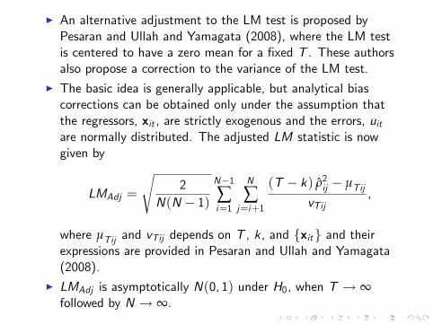
I An alternative adjustment to the LM test is proposed byPesaran and Ullah and Yamagata (2008), where the LM testis centered to have a zero mean for a xed T . These authorsalso propose a correction to the variance of the LM test.

I The basic idea is generally applicable, but analytical biascorrections can be obtained only under the assumption thatthe regressors, xit , are strictly exogenous and the errors, uitare normally distributed. The adjusted LM statistic is nowgiven by

LMAdj =

s2

N(N 1)N1∑i=1

N

∑j=i+1

(T k) ρ2ij µTijvTij

,

where µTij and vTij depends on T , k, and fxitg and theirexpressions are provided in Pesaran and Ullah and Yamagata(2008).

I LMAdj is asymptotically N(0, 1) under H0, when T ! ∞followed by N ! ∞.

I The application of the LMAdj test to dynamic panels or panelswith weakly exogenous regressors is further complicated bythe fact that the bias corrections depend on the true values ofthe unknown parameters and will be di¢ cult to implement.The implicit null of LM tests when T and N ! ∞, jointlyrather than sequentially could also di¤er from the null ofuncorrelatedness of all pair-wise correlations.

I To overcome some of these di¢ culties Pesaran (2004) hasproposed a test that has exactly mean zero for xed values ofT and N. This test is based on the average of pair-wisecorrelation coe¢ cients

CDP =

s2T

N(N 1)

N1∑i=1

N

∑j=i+1

ρij

!.

I As N,T ! ∞ in any order, CDP tends approximately to astandardized normal. One important advantage of the CDPtest is that it is applicable also to autoregressiveheterogeneous panels, even for a xed T , so long as uit aresymmetrically distributed around zero. The CD test can alsobe applied to unbalanced panels.

I Pesaran (2013) extends the analysis of CDP test and showsthat the implicit null of the test is that of weak cross-sectionaldependence and it depends on the relative expansion rates ofN and T .

I In particular, using the exponent of cross-sectionaldependence, α, developed in Bailey, Kapetanios and Pesaran(2011) and discussed above, Pesaran shows that whenT = O (Nε) for some 0 < ε 1 the implicit null of the CDPtest is given by 0 α < (2 ε) /4. This yields the range0 α < 1/4 when N,T ! ∞ at the same rate such thatT/N ! for some nite positive constant , and the range0 α < 1/2 when T is small relative to N.

I For larger values of α, as shown by Bailey, Kapetanios andPesaran (2011), α can be estimated consistently using thevariance of the cross-sectional averages.

I Monte Carlo experiments reported in Pesaran (2013) showthat the CD test has good small sample properties for valuesof α in the range 0 α 1/4, even in cases where regressorsare weakly exogenous.

I Other statistics have also been proposed in the literature totest for zero contemporaneous correlation in the errors uit .

I Using results from the literature on spacing discussed in Pyke(1965), Ng (2006) considers a statistic based on the qth

di¤erences of the cumulative normal distribution associated tothe N(N 1)/2 pair-wise correlation coe¢ cients orderedfrom the smallest to the largest, in absolute value.

I Building on the work of John (1971), and under theassumption of normal disturbances, strictly exogenousregressors, and homogenous slopes, Baltagi, Feng and Kao(2011) propose a test of the null hypothesis of sphericity,dened by HBFK0 : ut IIDN

0, σ2uIN

. Joint assumption of

homoskedastic errors and homogenous slopes is quiterestrictive in applied work and therefore the use of the JBFKstatistics as a test of cross-sectional dependence should beapproached with care.

Conclusions

I We have characterized the cross-sectional dependence as weakor strong, and dened the exponent of cross-sectionaldependence, α.

I We have also considered estimation and inference on largepanels with a factor error structure. We have distinguishedbetween panels with strictly exogenous regressors and dynamicpanels.

I Last but not least, we have provided an overview of theliterature on tests of error cross-sectional dependence when Nis large and units are unordered.

Reading list

This lecture is based on the following survey paper:

I Chudik, A. and M. H. Pesaran (2013a). Large Panel DataModels with Cross-Sectional Dependence: A Survey. Mimeo,May 2013.

For further reading on the topics covered in this lecture, seethe following papers.- On the types of cross-sectional dependence:

I Chudik, A., M. H. Pesaran, and E. Tosetti (2011). Weak andstrong cross section dependence and estimation of largepanels. The Econometrics Journal 14, C45C90.

I Bailey, N., G. Kapetanios, and M. H. Pesaran (2012).Exponents of cross-sectional dependence: Estimation andinference. CESifo Working Paper No. 3722, revised October2012.

- On the estimation and inference on large panels withstrictly exogenous regressors and a factor error structure:(a) PC methods

I Coakley, J., A. M. Fuertes, and R. Smith (2002). A principalcomponents approach to cross-section dependence in panels.Birkbeck College Discussion Paper 01/2002.

I Bai, J. (2009). Panel data models with interactive xede¤ects. Econometrica 77, 12291279.

(b) CCE approachI Pesaran, M. H. (2006). Estimation and inference in largeheterogenous panels with multifactor error structure.Econometrica 74, 9671012.

Extensions of CCE approach:

I Chudik, A., M. H. Pesaran, and E. Tosetti (2011). Weak andstrong cross section dependence and estimation of largepanels. The Econometrics Journal 14, C45C90

I Kapetanios, G., M. H. Pesaran, and T. Yagamata (2011).Panels with nonstationary multifactor error structures. Journalof Econometrics 160, 326348.

I Pesaran, M. H. and E. Tosetti (2011). Large panels withcommon factors and spatial correlation. Journal ofEconometrics 161 (2), 182202.

(c) Monte Carlo studyI Coakley, J., A. M. Fuertes, and R. Smith (2006). Unobservedheterogeneity in panel time series. Computational Statisticsand Data Analysis 50, 23612380.

- On the estimation and inference on large dynamic paneldata models with a factor error structure:(a) QMLE approachI Moon, H. R. and M. Weidner (2010a). Dynamic linear panelregression models with interactive xed e¤ects. Mimeo, July2010.

I Moon, H. R. and M. Weidner (2010b). Linear regression forpanel with unknown number of factors as interactive xede¤ects. Mimeo, July 2010.

(b) PC approachI Song, M. (2013). Asymptotic theory for dynamicheterogeneous panels with cross-sectional dependence and itsapplications. Mimeo, 30 January 2013.

(c) CCE approachI Chudik, A. and M. H. Pesaran (2013b). Common correlatede¤ects estimation of heterogeneous dynamic panel datamodels with weakly exogenous regressors. CESifo WorkingPaper No. 4232.

- On the tests of error cross-sectional dependence:

I Pesaran, M. H. (2004). General diagnostic tests for crosssection dependence in panels. CESifo Working Paper No.1229.

I Pesaran, M. H. (2013). Testing weak cross-sectionaldependence in large panels. forthcoming in EconometricReviews.

I Pesaran, M. H., A. Ullah, and T. Yamagata (2008). Abias-adjusted LM test of error cross section independence.The Econometrics Journal 11, 105127.