large eddy simulation of atmospheric convection on mars

Q. J. R. Meteorol. Soc. (2002), 128, pp. 1–999 doi: 10.1256/qj.02.169

Large eddy simulation of atmospheric convection on Mars

By TIMOTHY I. MICHAELS�

and SCOT C. R. RAFKINSouthwest Research Institute, USA

(Received 1 January 2000; revised 31 January 2001)

SUMMARY

Large Eddy Simulations are performed using the Mars Regional Atmospheric Modeling System (a non-hydrostatic, mesoscale model) in order to obtain a detailed, three-dimensional understanding of the daytime Marsatmospheric boundary layer. These microscale runs utilize the full radiative transfer (including a static dust profile)routines of the mesoscale model and a multi-level, prognostic subsurface thermal model. Surface albedo, thermalinertia, Coriolis parameter, and solar forcing are homogeneously set to values at the Mars Pathfinder landing site�19.33°N, 33.55°W (IAU1991); L � = 143° � . The initial state is obtained from a previous mesoscale simulation,

and is representative of the Mars Pathfinder landing site during summer.The convective boundary layer of Mars is found to exhibit structures and turbulent statistics outwardly

similar to that of Earth’s convective boundary layer. However, direct infrared radiative heating of the near-surfaceatmosphere is the primary mechanism for the transfer of energy from the solar-heated surface, and affects thebehaviour of the convection. Mars convection is more intense than that on Earth, primarily due to lesser gravity andatmospheric mass. Also, certain empirical scaling constants within the subgrid-scale turbulence parametrization(originally developed for terrestrial Large Eddy Simulations) appear to require significant reduction in order forthe scheme to perform adequately on Mars. The simulation results are used to further meaningfully interpretspacecraft images of convective clouds. The results also compare favourably with Mars Pathfinder in situmeteorological measurements, and help reconcile large daytime variances in that dataset.

KEYWORDS: Convective boundary layer Dust devils Subgrid-scale turbulence parametrization

1. INTRODUCTION

The structure and dynamics of the Mars atmospheric boundary layer (ABL) areneither well known nor well understood. However, the complex processes and motionswithin this lowest region of the atmosphere directly impact the descent and landedphases of all surface-based Mars missions, regardless of whether they are robotic ormanned. Furthermore, the processes that cause aeolian erosion of landforms, raise andredeposit dust, and allow for the surface deposition and sublimation of water and carbondioxide ices all occur within the ABL. This region of the atmosphere also providesa primary energy conduit through which solar energy drives the large-scale generalcirculation. Thus it appears that investigation of the Martian ABL is well-warranted.A summary of past work and the current state of knowledge pertaining to this topicfollows.

(a) Spacecraft measurementsThe twin Viking Lander spacecraft provided the first in situ measurements of the

near-surface Mars atmosphere in 1976. This data was examined by Sutton et al. (1978),who concluded that the likely daytime ABL, or convective boundary layer (CBL), depthat the Viking 1 Lander site during summer is 4-5 km, the maximum daytime surfacesensible heat flux is 15-20 W m �� , and low-level convection is three times as vigorousas its terrestrial counterpart. Although the results of such studies are important andquite useful, one must not lose sight of the fact that such quantities are very difficult tomeasure, even on Earth, and that many assumptions and/or approximations (e.g., surfacetemperature determination method, use of scaling laws developed for Earth, instrumentuncertainties, etc.) were made in order to indirectly arrive at these quantities. OtherViking-era evidence of Mars CBL depth and structure includes large dust devils up to�

Corresponding author: Southwest Research Institute, 1050 Walnut St, Suite 400, Boulder, CO 80302, USA.© Royal Meteorological Society, 2002.

1

2 T. I. MICHAELS and S. C. R. RAFKIN

7 km in height (Thomas and Gierasch 1985) and convective cloud streets (Briggs et al.1977) captured in Viking Orbiter spacecraft imagery.

Mars Pathfinder (MPF) collected in 1997 the most recent and highest temporalresolution in situ dataset yet. MPF results (Schofield et al. 1997) confirmed the presenceof strong near-surface temperature gradients, chronicled the passage of dust devils andother convective structures over the lander, and suggested that the turbulent powerspectrum of Mars’ atmosphere is similar to that of Earth in some conditions. Also, small(on the order of 100 m in diameter) nearby dust devils were discovered in MPF imagery(Metzger et al. 1999), offering yet another clue to the structure of the Mars CBL.

Recent imagery from the Mars Orbiter Camera (MOC) aboard the Mars GlobalSurveyor (MGS) spacecraft has improved our indirect knowledge of the CBL. Severalintermediate-size dust devils have been imaged by MOC at high resolution. Numerousdust devil tracks are visible on much of the planet’s surface, often exhibiting complexloops and turns that are indicative of the dynamical CBL processes that the phenomenawere embedded in (Malin and Edgett 2001). Convective cloud streets have been imagedin greater detail than before (Wang and Ingersoll 2002). Convective structures are evenrevealed in detailed MOC images of dust plumes. These data only offer hints at thenature of the CBL, as it remains invisible for the most part.

(b) Analytical and numerical modeling studiesThe work of Goody and Belton (1967) implied that Mars might have a relatively

deep ABL compared to that of Earth (the terrestrial ABL depth is typically 1-3 km),owing to the short radiative time constant of the Martian atmosphere. A one-dimensional(1-D) analytical and numerical study conducted by Blumsack et al. (1973) concludedthat the daytime ABL (also known as the convective boundary layer, or CBL) on Marsis likely 3-15 km in depth. It was emphasized that the gross ABL structure appearsto be controlled primarily by the radiative heating of the lowest few kilometers dueto upwelling infrared energy from the surface � further supported by the later work ofHaberle et al. (1993) and Savijarvi (1991) � . An early three-dimensional (3-D) Marsgeneral circulation model (without direct solar heating of suspended dust) attained amaximum CBL depth of 6-8 km (Pollack et al. 1976).

Ye et al. (1990) applied improved analytical techniques and two-dimensional (2-D) numerical modeling to the problem, and concluded that the Martian CBL is likely3-4 times deeper, has a smaller daytime surface sensible heat flux (15-30 W m �� ), andexhibits a representative eddy mixing coefficient ten times larger (i.e., convection ismore vigorous) than the terrestrial CBL. Subsequent modeling studies using variousone-, two- and three-dimensional numerical models (Savijarvi and Siili 1993; Haberle etal. 1993; Savijarvi 1995) yielded values similar to the Viking results. Model simulationsof the Mars Pathfinder atmosphere attained CBL depths of 4-5 km and satisfactorilysimulated the near-surface temperature measurements (Savijarvi 1999; Haberle et al.1999).

However, it must be noted that the above work was carried out using surface layertheories and largely empirical bulk turbulence parametrizations developed for Earth’satmosphere. It has not been rigorously shown that these methods are universal for allatmospheres similar to the terrestrial one (e.g., Mars’ atmosphere). Furthermore, theseparametrizations often do not accurately reflect the detailed effects of CBL turbulence,even on Earth. In order to examine the Mars CBL with the least practical amount ofparametrization and thus presumably with less error, a Large Eddy Simulation (LES)may be performed. The LES method attempts to explicitly resolve all of the important,larger turbulent motions that transport the vast majority of energy in the CBL, while

MARS ATMOSPHERIC CONVECTION 3

parametrizing the small turbulent motions that primarily act to diffuse and dissipateenergy.

The pioneering terrestrial LES work was by Deardorff (1972). That first investi-gation compared relatively well with available observations. However, computationalpower proved to be a severely limiting factor, and little additional numerical workwas published until the mid-1980s, when computers had improved sufficiently. By theclose of that decade, the primary structure of the convective boundary layer had beendescribed in detail (Schmidt and Schumann 1989), though there are a paucity of ob-servations to compare those results to. Briefly, the buoyantly-driven ABL is seen todevelop quasi-steady cellular updraught/downdraught structures, roughly hexagonal inshape, with narrow, intense updraughts surrounding much wider and less intense down-draughts. As computer capability continued to improve, additional investigations wereconducted, such as comparing shear- and buoyancy-driven ABLs (Moeng and Sullivan1994). The widening of the cellular structures with time in LES has been noted byFiedler and Khairoutdinov (1994) and Dornbrack (1997). Recently, Kanak et al. (2000)has laid the groundwork for the numerical investigation of small-scale vortices in theEarth’s CBL (e.g., dust devils). Also, the terrestrial version of the model modified (forMars) for use in this study has been used successfully for LES (e.g., Hadfield et al. 1991;Walko et al. 1992).

Studies of the Mars atmosphere using a 2-D LES (Odaka et al. 1998; Odaka 2001)predict vigorous turbulent mixing to a depth of approximately 10 km in the Mars CBL. Aprevious 3-D LES simulation using an early version of the Mars Regional AtmosphericModeling System (MRAMS) predicted a maximum CBL depth of 7 km, quite vigorousconvection, and possible dust devil circulations (Rafkin et al. 2001). At the time ofwriting, there are no other independently published 3-D Mars LES works.

(c) Current state of knowledge and the present approachBased on results and conclusions from previous work, the overall consensus appears

to be the following: The maximum depth of the Mars CBL varies with season andlocation but generally is in the range of 3-8 km. Dust devils appear to be ubiquitousat many scales in the CBL, and can be several times larger than their terrestrialcounterparts. Convective cloud streets appear to be similar to those associated withEarth’s CBL, implying that the overall structure of Mars convection is similar as well.Turbulence is more vigorous due in part to the lesser gravity and thin atmosphere ofMars. There exist present-day mechanisms for lifting dust in the Mars CBL, proven inpart by the existence of dust devils, their tracks on the surface, and the non-permanenceof those tracks. Radiative heating of the lowest kilometer of the atmosphere is likelyan important mechanism in the Mars CBL, and contrasts strongly with the heatingmechanism of the Earth CBL. Surface layer theories developed for Earth appear to bevalid (or at least similar) for Mars as well, according to MPF measurements (Schofieldet al. 1997).

The present study is undertaken to simulate and investigate the three-dimensionalprocesses and structure of the Mars CBL using MRAMS large eddy simulations. Thisstudy has the following three goals:

(1) Determine the three-dimensional structure of the Mars CBL under low wind-shear conditions, and compare with the structure of the Earth’s CBL.

(2) Quantify the turbulent statistics of the 3-D Mars CBL.


(3) Compare LES results with spacecraft measurements and images, in order to gainconfidence in the model solution and offer insight on how to more fully interpret thosedata.

2. METHODOLOGY

(a) Numerical model descriptionThe model employed in this study is the Mars Regional Atmospheric Modeling

System. In brief, MRAMS is a non-hydrostatic, finite-difference, limited domain (withoptional nested domains), mesoscale model designed to simulate the atmosphere ofMars. It is an improved version of the model described and used by Rafkin et al. (2001).Details pertaining to the recent model modifications may be found in Michaels (2002).For the present purpose, however, only the modifications made to the subgrid-scale(SGS) turbulence parametrization used in the LES are relevant.

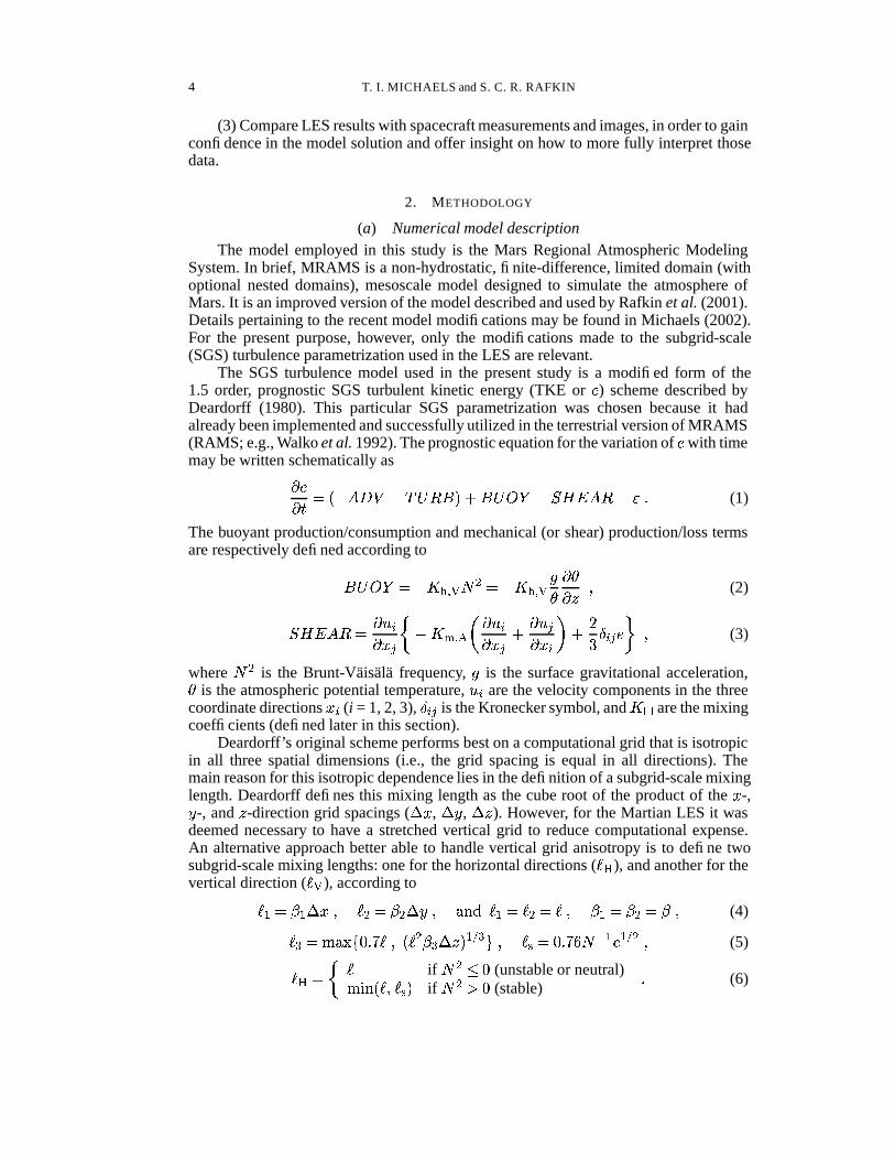
The SGS turbulence model used in the present study is a modified form of the1.5 order, prognostic SGS turbulent kinetic energy (TKE or � ) scheme described byDeardorff (1980). This particular SGS parametrization was chosen because it hadalready been implemented and successfully utilized in the terrestrial version of MRAMS(RAMS; e.g., Walko et al. 1992). The prognostic equation for the variation of � with timemay be written schematically as� �� "!$#&%� ��('*) (1)

The buoyant production/consumption and mechanical (or shear) production/loss termsare respectively defined according to

��+��,�-/. 0$1 � �+�2,�-/. 0234 � 4�6587 (2)

!$#&%� �9� ��:<;�6=?> @ �(,BA . CED �6:6;�6=?>E� ��:F>�6=6;HGI�KJLNM ;O> �FP 7 (3)

where 1 � is the Brunt-Vaisala frequency, 3 is the surface gravitational acceleration,4is the atmospheric potential temperature,

:�;are the velocity components in the three

coordinate directions=Q;

(i = 1, 2, 3), M ;O> is the Kronecker symbol, and ,�R are the mixingcoefficients (defined later in this section).

Deardorff’s original scheme performs best on a computational grid that is isotropicin all three spatial dimensions (i.e., the grid spacing is equal in all directions). Themain reason for this isotropic dependence lies in the definition of a subgrid-scale mixinglength. Deardorff defines this mixing length as the cube root of the product of the

=-,S -, and

5-direction grid spacings ( T = , T S , T 5 ). However, for the Martian LES it was

deemed necessary to have a stretched vertical grid to reduce computational expense.An alternative approach better able to handle vertical grid anisotropy is to define twosubgrid-scale mixing lengths: one for the horizontal directions ( U/V ), and another for thevertical direction ( U 0 ), according toU/W �IX WYT = 7 U � �IX � T S 7 Z\[�] U^W � U � � U 7 X W �IX � ��X 7 (4)U`_ �ba Z/c �ed )gf U 7 � U � X _hT 5 � Wji _ � 7 Ulk � d )gfHmH1 � W � Wji � 7 (5)

U V � @ U if 1 �on d (unstable or neutral)a�p [ � U 7 U`k � if 1 �oq d (stable)7 (6)


U 0 � @ U`_ if 1 � n d (unstable or neutral)a�p [ � U _ 7 Ulk � if 1 � q d (stable)7 (7)

where X and X _ are scaling constants (discussed in more detail later in this section).The lower limit for U _ (Eq. 5) was chosen arbitrarily to prevent the vertical mixing frombeing insufficient where T 5 is small (near the surface).

The SGS mixing lengths defined above are used with the turbulent Prandtl number(��

) to calculate the mixing coefficients for horizontal momentum, horizontal scalars,average momentum, vertical momentum, and vertical scalars,,BA . V ��,�-/. V � d )�� Wji � U V 7 ,BA . C � d )�� Wji � � U`VNU`VNU 0 � Wji _ 7 (8), A . 0 � d )�� U 0 � Wji � 7 ,B-/. 0 ��, A . 0�� , A . 0 � � � J � U 0�� U _ � � 7 (9)

respectively. Note that in the shear term of the prognostic calculation of subgrid-scaleTKE (Eq. 3), Deardorff’s definition of the mixing length is retained (within , A . C ),since it does contain information (however muted) about the full dimensions of eachgrid cube.

Viscous dissipation ( ' ) is parametrized by

'o� � _ i �� U V U V U 0 � Wji _ 7 � �� d )��2� d )�� D U V U V U 0U W U � U _ GWji _ 7 (10)

except in the lowest model layer (nearest the surface) where � L )�� , as suggestedin Deardorff (1980) and elsewhere to better handle “wall effects”. � � is the 3-Dadvection of � by the resolved-scale wind, and �� is primarily the subgrid-scaletransport (diffusion; uses the mixing coefficients given above) of � by small turbulenteddies (also implicitly includes the “pressure correlation” term of the full TKE tendencyequation). The latter two terms are calculated outside of the SGS model (detailed inRafkin et al. 2001).

It was found through preliminary numerical experiments that the values for thescaling constants ( X and X _ ), which in practice have a value equal to or slightly greaterthan unity on Earth, needed to be decreased by a factor of at least three (scaling constantsused in this work are X � d )��ef , X _ � d )�� ) in order to avoid overdiffusing (i.e., noconvective motions are able to develop at any time during the day) the model solution forMars. If the scaling constants (and thus ultimately the mixing coefficients) are too large,resolved-scale convection fails to initiate, and instead a very quiescent ABL developsdue solely to the accumulated action of subgrid-scale diffusion. If the scaling constantsare made too small, numerical noise (“2 T = ” noise) quickly develops and dominates themodel solution. Many combinations of scaling values were tried, including pairs whereX _ was much greater than X , and vice versa. It was found that the horizontal scalingconstant ( X ) effectively controlled the timing of the onset of resolved-scale convectionand the damping of numerical noise. In stark contrast, the model solution appeared to bemuch less sensitive to the value given to the vertical scaling constant. The significanceof these observations is uncertain.

(b) Numerical experiment designTwo separate LES were performed at different horizontal and vertical resolutions.

This was done in order to better understand the impact of model grid spacing onthe resulting solution, to attempt to resolve convective structures more clearly, and toelucidate the characteristics of the flow at and during the onset of ABL convection.


Both simulations were initialized in exactly the same manner, and used the same modelphysics and parametrizations. However, due to finite time and computational resources,the computational grids of the simulations were not the same size, nor were theyintegrated over the same period of time.

The computational grid of Simulation 1 (hereafter referred to as S150) is 24 � 24km in the horizontal and approximately 9.5 km deep in the vertical. The horizontalgrid spacing is 150 m, and was chosen based on earlier two- and three-dimensionaltrial runs that indicated this value to be satisfactory for modeling the largest CBLeddies. The vertical grid was gradually stretched with height, with a first layer thicknessof 4 m (lowest level at about 1.9 m above the surface), increasing to a maximumof 225 m (1.5 times the horizontal grid spacing, in order to keep the bulk of thethree-dimensional computational grid approximately isotropic) aloft. These dimensionsrequire 160 � 160 � 61 grid points. The rationale for choosing the above grid dimensionsis that Mason (1989) postulated that a grid at least 3.2 times the width of an individualconvective cell was necessary to properly represent CBL statistics on Earth. Based onearlier tests (which suggested that Martian convective cells were 7 to 8 km wide) andcomputer limitations (both memory/storage and computational time needed), the abovedimensions were chosen – with the aim of having significant CBL statistics and realisticCBL structures and dynamics.

The computational grid of Simulation 2 (hereafter referred to as S30) is 6 � 6 km inthe horizontal and approximately 2.3 km deep in the vertical. The horizontal grid spacingis 30 m. The vertical grid is gradually stretched with height, with a first layer thicknessof 4 m (lowest level at about 1.9 m above the surface), increasing to a maximum of 45m aloft. These dimensions require 200 � 200 � 61 grid points.

All grids were made strictly Cartesian (i.e., no attention was paid to planetary cur-vature). Flat topography was assumed (i.e., topography was set to zero meters every-where). The entire domain of each simulation was assumed to be at the location of theMars Pathfinder landing site at the southern edge of Chryse Planitia � 19.33°N, 33.55°W(IAU1991 areographic coordinate system) � for the purpose of radiative computations.This also allows for a more meaningful comparison with actual landed MPF data. Ther-mal inertia and albedo were set to be constant over the entire grid (set to representativevalues from the MPF site: thermal inertia = 384.5 J K � W m �� s � Wji � , albedo = 0.197). Thesurface aerodynamic roughness length used was 0.03 meters. A static dust distributionwas used (dust concentration decreased roughly exponentially with height), with a dustoptical depth of 0.3 on a pressure surface of 6.1 hPa.

Cyclic (sometimes termed periodic) lateral boundary conditions were used forboth simulations, and effectively simulate an infinite planar domain. This type ofboundary condition was primarily chosen because there are no three-dimensional ABLobservations for Mars to use as boundary conditions and an appropriate mesoscalesimulation to provide boundary conditions was judged to be too time-intensive toundertake at present. Moreover, it is likely a reasonably good approximation to thesituation in the northern plains of Mars. Assuming a mean wind of 5 m s � W , theequivalent domain simulated during a solar convective day of 10 Mars-hours (about36990 s) is basically a flat plain 200 km wide with atmospheric convection occurringeverywhere. A plain of such a size is easily found near the MPF landing site. Atthe model top, a Rayleigh friction layer 5 vertical grid points thick was used with adissipation time-scale of one Mars-hour.

The Coriolis parameter was kept spatially constant (set to the value at 19.33°N)for both simulations. The full subsurface thermal model of MRAMS was used, aswell as the full radiation code (from the NASA Ames Mars general circulation model;


includes dust and carbon dioxide gas plane-parallel radiative transfer at visible/near-infrared wavelengths and in two infrared ranges). However, the use of cyclic boundaryconditions necessitated that the solar zenith angle be treated as if the entire grid was asingle point (the areographical location of the grid center). A radiative time step of 30 swas used in an attempt to capture the radiative changes induced by the largest convectiveABL eddies (since they may significantly alter the temperature/pressure profile over thatperiod of time). The starting season was approximately

� k � �� L °, which is the latterportion of the Northern Hemisphere summer. This season was chosen partly because thesynoptic scale disturbances should be weak at the MPF site (allowing for approximateatmospheric repeatability sol after sol), and secondly, this was the season that the MarsPathfinder spacecraft landed at, so the model results should compare well with thelanded observations.

Both simulations were initialized with a single sounding from a previous mesoscalesimulation of the MPF site. The initial fields were thus horizontally homogeneous.Only the sounding temperature and pressure profiles were used. Wind components werespecified as follows:

:= 5 m s� W , � = 0 m s � W , and � = 0 m s � W . Although there is no

initial wind shear, after the simulation begins friction with the surface quickly producesweak shear throughout the lowest several hundred meters of the CBL. This choice wasmade in order to examine the intrinsic structure (i.e., the weakly sheared structure) ofthe convective boundary layer on Mars, but still have a slight amount of mean wind inone direction to move the convective cells/phenomena across the domain (which addsrealism). The horizontally homogeneous potential temperature field from the soundingwas randomly perturbed by up to 0.1 K at the lowest model level in order to provide aslight amount of inhomogeneity to foster the onset of resolved convection.

Two generic 24 Mars-hour time systems are used in this work. The first, analogousto the terrestrial Coordinated Universal Time (UTC) system and shares the same name,defines 0000 UTC to be midnight at the 0°E meridian in the IAU1991 areographiccoordinate system. The second, Local Solar Time (LST), is offset from UTC by asimple linear function of areographic longitude analogous to local time on Earth. Bothsimulations were started at 0810 UTC (about 0556 LST), which is just after the localsunrise, in order to simulate the entire convective ABL evolution (achieved only inS150).

A dynamical time step of 2 s was required to keep S150 numerically stable afterresolved convection initiated, due to large vertical velocities across the relatively thinmodel layers near the surface. A fully three-dimensional snapshot of all prognosticvariables was archived every 300 simulated seconds. S150 was halted at 2020 UTC(1805 LST, 45000 s after start) after the ABL convection had almost completelydissipated. Similarly, a dynamical time step of 1 s was required to keep S30 numericallystable. Model output occurred every 180 s. S30 was halted at 1349 UTC (1134 LST,20880 s after start) after it was judged that the convective cells were becoming too largefor the grid.

3. RESULTS

(a) Spatial and dynamic CBL structure

(i) Convective cells. Loss of momentum to the ground (due to friction) quickly createsnear-surface speed shear in the initially vertically homogeneous wind profile. Soon after,the surface/air interface becomes warmer than the immediately overlying air (due toinsolation), and atmospheric convection ensues (as the fluid’s natural way to cool its


lower boundary). The convective boundary layer initially evolves purely due to subgrid-scale (SGS) turbulence, evidenced by a deepening layer of greatly increased SGSturbulent kinetic energy (the only SGS quantity truly prognosed by the model) boundedby the surface and having no resolved spatial perturbations in wind, temperature, orpressure. When this SGS CBL attains a depth roughly equal to three times the horizontalgrid spacing, resolved-scale convection initiates and immediately dominates the SGSprocesses (by an order of magnitude or more in terms of turbulent energy fluxes). Thisdisparity between the magnitude of the SGS and resolved-scale fluxes at nearly the sametime of sol is noteworthy, as it suggests that the SGS parametrization is not adequatelyrepresenting the real-world SGS turbulence intensity (discussed further in Section 3b).The CBL depth at which this transition takes place is strongly a function of the strengthof the horizontal SGS diffusion in the model. SGS diffusion was tuned to initiateresolved-scale convection at approximately three times the horizontal grid spacing sincethe model cannot properly treat turbulent eddies smaller than that (assuming the saideddies are all quasi-isotropic).

Resolved-scale convection begins as regularly spaced linear plumes of buoyant fluidaligned parallel to the mean shear vector (Fig. 1a). Note that updraughts and down-draughts occupy equal areas and have roughly equal magnitudes at this stage. However,in a near-surface (i.e., where there is vertical speed shear due to friction) environmentdominated by buoyant forces, rather than shear forces, such linear structures are notstable. In order to maintain such symmetric structures, the three-dimensional fluid flowmust somehow maintain an excruciating spatial symmetry, since any asymmetries willtend to amplify (because of momentum transport from aloft) or at least produce otherasymmetries in the flow. In the model solutions, the first returning fluid (i.e., fluid thathas journeyed upwards in one of the initial updraughts and has now returned to thesurface in a downdraught) exhibits spatial asymmetries in vorticity (generated alongthe updraught lines), momentum, and heat (perhaps in part caused by gravity waveinteractions along the upper boundary of the CBL) that warps sections of the linearupdraught/downdraught structures in directions roughly perpendicular to the mean shearvector. The warping causes sections of adjacent updraught structures to connect, form-ing elongated, closed loop updraught structures. As this process continues, the linearupdraught structures give way to roughly elliptical structures (Fig. 1b), which in turndivide into roughly circular structures (Fig. 1c). Also, downdraughts gradually encom-pass much more area and become weaker than updraughts. Finally, updraught strengthincreases dramatically during this period, as insolation, and thus the heating of the lowerboundary of the atmosphere (most importantly due to absorption of upwelling infraredradiation, and secondarily due to molecular thermal conduction from the surface) in-creases. The shape of the approximately circular convective structures, or cells, is oftenmore aptly described as polygonal (chiefly quadrilateral, pentagonal, and hexagonal).These polygonal cells persist throughout the remainder of the solar convective day.

The structure of these polygonal convective cells is startlingly complex and effi-cient. Every cell side is shared with an adjoining cell, so that there is no surface arealeft unencompassed. The cell sides are composed of relatively narrow and intense up-draughts, while the majority of the cell interior contains only broad, relatively weakdowndraughts. The lowest several hundred meters of each cell interior is a region ofdivergent flow towards the cell sides. Embedded in this low-level flow are much smallerconvective cells with a structure similar to their larger cousins. This smaller-scale con-vection, kept from growing larger by subsidence and shear due to descending air in thelarge-scale cell interior, serves to channel near-surface buoyant fluid from the interior ofthe cell outward to feed the larger-scale updraughts that make up the cell sides.


Figure 1. Horizontal cross-sections (each 6 � 6 km; � is vertical axis, � is horizontal axis) of S30 vertical velocity�filled areas are regions of upward (positive) velocity � at z = 25.4 m for: (a) 0749 LST, initiation of resolved-scale

convection, with contours at -0.01 and 0.01 m s ��; (b) 0804 LST, warping of linear convective features, with

contours at -0.2 and 0.1 m s ��; and (c) 0833 LST, early polygonal convective cells, with contours at -0.2 and 0.1

m s ��.

The Mars Orbiter Camera (MOC) aboard the Mars Global Surveyor (MGS) space-craft has frequently imaged what appear to be convective clouds over the Syria Planumregion of Mars (Wang and Ingersoll 2002). Figure 2a is a 48 � 48 km portion of sucha MOC image (M0104901, taken at approximately 1430 LST). Comparing the overallshapes and distribution of the white cloud areas in Fig. 2a with the contoured areas(regions of strong vertical velocity near the top of the S150 CBL at 1441 LST) of Fig.2b, there are striking similarities that appear to further confirm (albeit indirectly) thenature of these clouds, as well as providing a real-world partial validation of the LESresults (i.e., that regions of the Mars atmosphere exhibit convection of similar scale andstructure as the simulation). The approximate size, height (compared to cloud heightsestimated from cast shadows), spatial distribution, and lobed nature of the simulated


Figure 2. (a) Area (48 � 48 km) of presumed convective clouds over Syria Planum (portion of Mars OrbiterCamera image M0104901). Horizontal cross-sections (4 copies tiled to create an area of 48 � 48 km) of S150vertical velocity (filled areas are regions of velocity greater than 2 m s �

�) at 1441 LST and: (b) z = 4342 m; (c) z

= 2092 m; (d) z = 988 m; and (e) z = 385 m. Straight solid line in above horizontal sections indicates the locationof the vertical cross-section shown in Fig. 3 below.


Figure 3. Vertical (X-Z) cross-section of vertical velocity through the S150 domain (location indicated in Figs.2b-e by straight solid line) 1441 LST. The contour interval is 2 m s �

�, and dashed contours indicate negative

(descending) velocities.

updraught cores all compare well with the MOC image. These clouds’ morphologyand formation mechanism are quite similar to terrestrial “open” cellular convectiveclouds (Atkinson and Zhang 1996) that occur over warm ocean surfaces during cold-air outbreaks. A notable difference is that in the relatively dry atmosphere of Mars,condensation is only able to occur above the very strongest updraughts (at the verticesof the cellular structure), whereas the terrestrial cellular clouds are often seen to tracethe outline of the entire convective cell (not just the vertices), due to abundant watervapor.

The numerical simulation results provide detailed representative information aboutatmospheric structure invisible in the spacecraft image. Figure 2c shows the updraughtsorganized into large convective cells mid-way through the CBL (2092 m). Updraughtintensity within the cell walls is not uniform. Descending to 988 m, Fig. 2d illustrateshow the convective cells become smaller and more distinct, and their constituentupdraughts narrower (and also less intense) near the surface. At a height of 385 m(Fig. 2e), a multitude of small, rapidly changing updraught structures are present,transporting highly buoyant fluid away from the surface. A west-to-east vertical cross-section (of vertical velocity) through the domain at the same time is shown in Fig. 3. Theproportions of this figure are 1:1 (i.e., no vertical exaggeration). Several deep updraughtsare visible, along with shallow updraughts and the broad downdraughts.

The mean size of all scales of convective cells broadens continuously throughoutthe day. This occurs at a pace dictated by the current available insolation and verticaltemperature and momentum structure of the atmosphere (i.e., the cells may broadenvery rapidly if a marginally stable layer of the atmosphere lies above them or if alayer of heightened momentum aloft is encountered and is then brought down to thesurface). The overall mechanism that causes the cells to broaden appears to be simplyconservation of mass (i.e., if there is more mass going up per unit time, there shouldalso be correspondingly more mass per unit time descending to take its place, and viceversa).

Figure 4a shows the mean (averaged over the entire horizontal domain) potentialtemperature profiles of S150 and S30 at roughly the same time in the morning. S30 hasdeveloped a profile that is more than 2 K cooler than S150 throughout most of the CBL.S30 also displays the warmest potential temperature near the surface. The net result is


Figure 4. Potential temperature (using a reference pressure of 1000 hPa): (a) Comparison of mid-morning meanprofiles. (b) Several representative, instantaneous S150 profiles at 1042 LST.

that S30 is significantly more superadiabatic at low levels than S150. Also, note thatS30 exhibits a slightly shallower CBL than S150. In both simulations, the mean profileis superadiabatic for fully half of the depth of the CBL, implying that convection is notefficient enough to overcome radiative heating from below. This structure is deceiving,however, since most of the domain is populated by downdraughts whose potentialtemperature profiles are nearly adiabatic throughout most of the CBL (Fig. 4b). Theextreme profiles of the narrow and deep large-scale updraughts are solely responsiblefor the shape of the mean profile. The profile through a shallow updraught in the interiorof a convective cell differs from the downdraught profile only in that the lowest levelsare very warm compared to even the deep updraught. Also note in Fig. 4b that theCBL depth in the downdraught is significantly less than in the two updraught profiles.Finally, the shape of the deep updraught profile indicates that the buoyant fluid is ableto rise relatively adiabatically and unentrained (i.e., without mixing much with coolerfluid) through much of the depth of the CBL.

The Mars LES work of Odaka (2001) utilizes a 2-D anelastic numerical model withno radiatively active atmospheric dust, but nevertheless may be qualitatively comparedto the present results. The large-scale structure of the convective eddies are quitesimilar, even though those of Odaka exhibit a greater vertical extent (10 km). Theapproximate maximum wind speeds seen by Odaka � max � : 7 � �� J d m s � W , � �

L d ms � W � are roughly twice the wind magnitudes seen in either S30 or S150. However, thesedifferences may be due in part to the 2-D nature of Odaka’s work, as 2-D LES lack theability to stretch vorticity. Preliminary MRAMS 2-D simulations using the present SGSformulation are seen to exhibit a deeper CBL and stronger winds than a corresponding3-D simulation. Additionally, the mean potential temperature profiles of Odaka’s resultsreveal a superadiabatic layer several hundred meters in depth (bounded by the surface),which compares well with MRAMS results (Fig. 4a).

(ii) Vertical convective vortices. Convective vortices known as dust devils are knownto be common across plains during the daytime on Mars (Ryan and Lucich 1983;Thomas and Gierasch 1985; Murphy and Nelli 2002). Specimens as large as 1 kmin width and 7 km tall have been seen in orbital imagery. Viking Lander and MarsPathfinder meteorology instruments have recorded several suspected small dust devilspassing over or near them (Schofield et al. 1997). Small dust devils have also been found


in Mars Pathfinder lander imagery (Metzger et al. 1999). Given dust devils’ often largesize and apparent ubiquity at many places on Mars, it seems probable that they maybe modeled in a Mars LES simulation. An LES such as S30 or even S150 should inprinciple be able to capture these atmospheric phenomena.

It is important to realize that a given dust devil circulation may not be visible tothe unaided eye if there is no dust to entrain, the circulation does not extend fully to thesurface, or if the circulation is too weak to entrain dust. In such cases, the circulation ismore generally referred to as a vertical convective vortex. Also, the fine details of thedust devil circulation, especially near the ground, occur at quite small scales, and thuswill not be resolved in any current LES. Finally, the structure, dynamics, and evolutionof dust devils on both Earth (Sinclair 1969, 1973) and Mars are not well known. Thelarge size of Martian dust devils may enable them to be simulated and studied withgreater ease and the results applied by analogy to the study of the often much smallerterrestrial variety.

Additionally, both S30 and S150 simulation results contain abundant vertical con-vective vortices at many different spatial scales (several kilometers to several hundredmeters in diameter) throughout the convective day that do not extend sufficiently nearthe surface (within about 100 meters) to be considered dust devils. In fact, the candidatedust devil circulations appear to comprise but a small subset of the total population ofCBL vertical vortices. Thus these observationally “invisible” vortices appear to be animportant part of the overall CBL structure on Mars � the work of Kanak et al. (2000)suggests a similar reality in the terrestrial CBL � . Preliminary examinations of the LESresults appear to indicate that the vorticity of the simulated vertical convective vortices(including dust devils) is first generated baroclinically along updraught lines as hori-zontal relative vorticity, then concentrated (via horizontal convergence), tilted into thevertical, and stretched at the convective cell vertices.

Surface-based convective vortices (i.e., dust devil candidates or DDC) were foundin both S30 and S150, beginning shortly after resolved-scale convection initiated andending when the large-scale convection began to collapse. It must be noted that S150and S30 utilize no dust lifting parametrization, and thus do not provide any quantitativeway of determining whether a given convective vortex in the model solution shouldbe termed a dust devil. The strongest and largest vertical vortices occurred during theearly afternoon, when convection is at its maximum intensity. The DDC vertical vorticesnearly always occurred along large-scale convective cell boundaries (updraughts), andthe most intense of these vortices occurred at the vertices of the polygonal convectivecell pattern. Near-surface wind speeds in the modeled DDC vortices were local maxima(on the order of 10 m s � W ), but not significantly greater than speed maxima caused bylarger-scale processes. Distinct negative pressure perturbations (up to about 2 Pa) wereassociated with all of the mature DDC vortex circulations (as in Rafkin et al. 2001).The magnitude of this pressure drop compares well (after considering the difference inambient atmospheric pressure) with measurements of Earth dust devils which exhibitperturbations of about 2 hPa. Calculations performed for a number of the modeledDDC circulations indicated that they are very nearly cyclostrophically balanced, with noobvious preferred direction of rotation. Many of the modeled DDC vortex circulationswere found to attain heights of 60% of the CBL depth or more.

An example of a simulated DDC vertical convective vortex is shown in the nextseveral figures. Figure 5a is a plot of the horizontal streamlines (1.9 m; the mean windhas been subtracted from the wind components) for a vortex that was present in S30at 1112 LST. Note that convective vortices at this time of day are not near their peakintensity and size. The anticyclonic vortex is approximately 200 m wide at its base,


Figure 5. Horizontal cross-sections of a S30 convective vortex at 1112 LST and z = 1.9 m: (a) streamlines (meanwind removed); and (b) contours of pressure (hPa).


and widens and tilts toward the northeast somewhat with height. This vortex is onlyabout 500 m deep, and if it were dust-laden, an observer would likely describe it asa wedge-type dust devil. Figure 5b illustrates the perturbation imposed on the totalpressure field by the same vortex, which is quite small (about 0.55 Pa), but neverthelessis unambiguously present. This vortex lies along and is embedded in one of the narrow,quasi-linear updraught features. Due to a mean west to east wind, the northern halfof this vortex exhibits the most intense wind (constructive interference). A west-eastvertical cross-section of three-dimensional relative vorticity magnitude through thevortex is shown in Fig. 6a. The vortex clearly tilts with height. Figure 6b shows a similarcross-section of vertical velocity, illustrating how the convective vortex is embedded ina much larger-scale buoyant plume. Note that the maximum vertical velocity is locatedalong the leading edge of the vortex (movement is from left to right), whereas the trailingedge is composed of a much weaker updraught.

(b) Turbulent statisticsIn light of the fact that the CBL is rife with many similar, ever-changing three-

dimensional structures, it is instructive to compute a number of statistics about the flow(e.g., covariances, variances, skewness, mean profiles). For a detailed description of thestatistical methods and assumptions used here, refer to Chapter 2 of Stull (1988). Suchstatistics provide a two-dimensional view (height and time) of the overall effects ofthe complex convective flows. All turbulent statistics presented here are computed as asingle vertical profile for each model output time, with each profile point being assignedthe average of that quantity over the entire horizontal domain at that level.

A time-height plot of the covariance of vertical velocity and temperature (a quantityproportional to the turbulent heat flux) from S150 is shown in Fig. 7a. Clearly, resolved-scale convection does not initiate in S150 until after 0930 LST. The entrainment zoneabove the CBL is plainly evident, growing deeper and more intense as the convectiveelements become larger and more energetic. The maximum value of 1.42 K m s � Wis reached at 1300 LST (just after the time of maximum insolation), and is nearlyan order of magnitude greater than maximum values measured in terrestrial desertatmosphere studies such as Schneider (1991). However, the maximum actual thermalenergy flux, which is obtained by multiplying the covariance by the air density and heatcapacity, is nearly an order of magnitude less than that on Earth, owing to the Martianair density being nearly two orders of magnitude smaller than on Earth. Since Marsreceives approximately half the terrestrial amount of solar insolation, the Martian CBLmust be more vigorous and deeper than the terrestrial CBL, due to the fact that theMartian atmosphere is so much less efficient at transporting heat. More intriguing isthe presence in the mean statistics of what appear to be regular pulses of convectiveactivity (especially evident in the entrainment zone; several can be seen in Fig. 7a –three between 1000 and 1100 LST, and two others centered at 1300 and 1415 LST) thatbecome more intense but less frequent as the day passes. This suggests that all (or at leastmost) of the convective cells in the domain are involved in a concerted (i.e., not random)cycle of overturning. Finally, the amount of vertical heat transport diminishes graduallythroughout the afternoon, until convection collapses completely sometime after 1700LST.

The time-height profile of S150 turbulent kinetic energy (TKE) provides a similarperspective (not shown). The maximum depth of the CBL, when defined as the regionof relatively high TKE bounded by the ground, is about 6 to 7 kilometers. The MRAMSTKE values are two to three times greater than in the typical terrestrial desert atmos-phere. The intensity of the CBL circulations is greatest at around 1400 LST. After 1600


Figure 6. X-Z vertical sections (y = 35) through the vortex shown in Fig. 5: (a) Three-dimensional relativevorticity magnitude (rad s �

�); and (b) vertical velocity (m s �

�, solid contours), dashed contours in lower center

are relative vertical vorticity – intended only to show vortex location.


Figure 7. Time-height sections of the covariance of vertical velocity and temperature (units of K m s ��, contours

are not all equally spaced) for: (a) entire length of the S150 simulation (dashed contours indicate negative values);and (b) entire length of the S30 simulation (solid), plotted atop the corresponding S150 results (dashed).


LST, the CBL eddies rapidly lose strength and have effectively collapsed by 1730 LST.The majority of the resolved-scale turbulent kinetic energy in the Martian CBL appearsto be contributed by vertical motions (as indicated by the comparison of perturbationvelocity values in the vertical with those in the horizontal). This suggests that the large-scale Martian convective eddies are strongly anisotropic (in intensity).

The vertical flux of horizontal momentum (the covariance of the horizontal andvertical velocities) is not shown, but worth noting. The values of this statistic are slightlyless than analogous measurements on Earth. Alternating (with time and height) positiveand negative values are a puzzling feature, as they indicate periods of mean gradient andcounter-gradient transport across the domain (as previously noted in Rafkin et al. 2001).Both individual covariances exhibit the same behavior, so the phenomenon is likely athree-dimensional process.

The next series of figures illustrate the differences between the statistics of S150and S30. Figure 7b shows the covariance of vertical velocity and temperature fromboth simulations. The height of the CBL becomes slightly shallower in S30 than S150,and is believed to be the result of changes in energy transport (caused by the higherresolution grid) and not boundary effects at the model top. The most obvious differenceis the location and intensity of the near-surface vertical gradient of the statistic. S30has covariance magnitudes similar to S150, but exhibits a much stronger gradient nearthe surface. This difference is exemplified by the profiles of S30 and S150 covariancesat approximately 0930 LST (immediately before resolved-scale convection begins inS150) shown in Fig. 8a. The S30 covariance is an order of magnitude or more greaterthan that of S150 throughout most of the CBL depth. Also, in S30 the SGS contributionis nearly two orders of magnitude less than the resolved one. In Earth LES studies,the resolved-scale covariance profile appears similar to that of S30. However, on Earth,the SGS contribution is quite significant near the surface, causing the total covarianceprofile (resolved+SGS) to be linear (negative slope) throughout the entire depth of theCBL. This profile shape indicates (via vertical heat flux divergence considerations)that convection on Earth acts to warm the atmosphere throughout the CBL. On Mars,the SGS contribution (as it is parametrized in this work) is negligible, and the lowestportion of the covariance profile exhibits a positive slope, indicating that near thesurface, resolved-scale convection is acting to cool the atmosphere. To make sense ofthis, consider that on Earth the atmosphere receives most of its energy via conductionfrom the surface, while on Mars the atmosphere likely receives most of its energy viathe absorption of upwelling infrared radiation from the surface � Mars’ atmosphere isrelatively opaque in certain regions of the infrared spectrum; see Haberle et al. (1993)and Savijarvi (1991) � . The role of convection in a fluid is to equalize the distributionof energy in the fluid, and as Mars’ atmosphere is significantly heated internally at lowlevels by radiation (not just at its lowest boundary via conduction), convection wouldnaturally act to cool the atmosphere in that region and warm the portion above.

Figure 8b shows the covariance profiles after both simulations have achievedresolved-scale convection. It clearly shows a difference in CBL depth and in near-surface structure between S30 and S150. A comparison of S30 and S150 TKE statisticsreveals a similar situation. This contrast is likely due to inadequacies of the SGSparametrization, as the total S150 covariance should be similar to the S30 results atthe same time and height if the SGS scheme were performing perfectly. Unfortunately,a parametrization is, by its very nature, an approximation, and therefore will likely neverperfectly represent its real-life or analytical counterpart. SGS parametrizations also donot perform ideally on Earth (e.g., Mason 1989), but this fact does not prevent terrestrialLES studies from drawing many meaningful conclusions. Thus, similar conclusions may


Figure 8. Comparisons of the S150 and S30 vertical profiles of the covariance of vertical velocity and tempera-ture (sum of resolved-scale and subgrid-scale contributions) for: (a) mid-morning; and (b) late-morning.


be also be made about the Mars CBL if the level of parametrization imperfection appearsto be of minimal importance to the robustness of key CBL structure and statistics. Suchappears to be the case, as the maximum and minimum values of the covariance (Fig. 8b)in both S30 and S150 are nearly identical, as are the qualitative shapes of the profiles.Furthermore, the large-scale convective structure of S30 and S150 are quite similar,and the MRAMS LES results compare well with high-resolution spacecraft images ofsmall-scale atmospheric phenomena (e.g., convective clouds), providing a measure ofqualitative model validation.

Figure 9b shows the vertical velocity skewness profiles of S30 and S150. Assumingthat the domain mean vertical velocity at each level is zero (in reality it is quite small),a positive value of this statistic indicates that updraughts are narrower than surroundingdowndraughts, and vice versa. The vertical velocity skewness is positive throughoutmost of the CBL, and has a maximum near the top of the CBL. Gravity (buoyancy)waves propagating along the top of the CBL are the reason for the sudden decrease abovethe maximum, since they have roughly equal areas of upward and downward velocity.Near the surface, the skewness becomes distinctly negative, indicating a tendency fornarrow downdraughts and broad rising motion there. These profiles are quite similar inall respects to Earth LES results, though those terrestrial results do not agree well withEarth observations (Moeng and Rotunno 1990). Also note the effect grid resolutionhas on the skewness profiles. Figure 9a shows a time-height plot of the S150 verticalvelocity skewness. It shows that throughout the convective day, the skewness profile isquite consistent until about 1630 LST, when skewness aloft decreases rapidly, indicatingthe collapse of the narrow updraughts. Also visible at approximately 1715 LST isthe reversal of the near-surface skewness from negative to positive, indicating broaddownward motion and narrow regions of upward motion. Nearly simultaneously, theskewness aloft also switches sign. These reversals appear to indicate the onset of thenocturnal ABL processes.

(c) Comparison to Mars Pathfinder (MPF) dataThe measured MPF temperature and wind time series have a rather large variance

during the day. This has been interpreted as primarily being the effects of daytimeconvection at the MPF site. If that is the case, the variance of the temperature and windtime series from the present LES simulations (at the MPF site) should compare wellwith the lander dataset. It is important to note, however, that with the possible exceptionof temperature, the mean magnitudes of the LES quantities cannot be expected to matchthose of the MPF observations, due to the partially idealized nature of the present LES(i.e., no topography or mesoscale pressure gradients). LES results are from S150 andare plotted every 300 s. The time resolution of the MPF data vary, but are generallyof higher time resolution than the LES results presented here. Finally, though the S30results will not be shown here, the variation that they exhibit is slightly greater than thatof the S150 results. Also, the MPF wind data shown in Fig. 10 have not yet been fullycalibrated. Even so, it is likely that most values are close to the fully calibrated values.

Figure 10a compares observed and modeled temperature at a height of 1.27 m abovethe surface. MRAMS temperatures here are simply linearly extrapolated from the lowestmodel level of 1.9 m. The MRAMS values are slightly colder than the MPF data, but doexhibit a variance of about 4 K (observed value is about 10K during mid-day).

Modeled and observed wind speeds are shown in Fig. 10c. Again MRAMS exhibitsa sizable amount of variation (about 7 m s � W ) due to convective motions. Also note thesteep drop (after the 25.7 time graduation) in the wind magnitude and variability afterthe large-scale convection collapses (seen also in the MPF dataset). A comparison of


Figure 9. Vertical velocity skewness (dimensionless): (a) S150 time-height section (dashed contours denotenegative values); and (b) comparison of late-morning S30 and S150 profiles.


Figure 10. Time series comparison of 1.27 m Mars Pathfinder (MPF) measurements (wind data provided by Dr.J. Murphy, New Mexico State University, USA) and extrapolated S150 results for: (a) temperature (black points,MPF; black line, S150); (b) wind direction (dark points, MPF; black asterisks, S150); and (c) wind speed (dark

points, MPF; black line, S150).


modeled and observed wind direction is shown in Fig. 10b. The amount of variationin the MRAMS wind direction compares well to the MPF data. Again note that afterconvection collapses, the wind direction becomes much more constant (borne out in theMPF data as well).

4. CONCLUSIONS

Two LES of the Martian atmosphere were performed using horizontal grid spacingsof 30 and 150 m. The convective boundary layer of Mars was found to exhibit large-scale structures and turbulent statistics outwardly similar to those in Earth’s CBL.Numerous convective vortices (including possible dust devils) were also present inboth simulations. MRAMS LES results compared well with high-resolution spacecraftimages of small-scale atmospheric phenomena, such as convective clouds, which attestto the existence of certain CBL structures. However, several key differences betweenthe CBL of Mars and Earth were noted: First, the lower atmosphere of Mars likelyreceives energy from the Sun primarily through the absorption of upwelling infraredradiation from the surface. This causes convection on Mars to cool the lower levels ofthe CBL and heat the remainder, whereas on Earth convection heats the entire CBL.Secondly, Mars’ lesser gravity, much lower atmospheric density (thus much less heattransport efficiency), and comparable amount of insolation (roughly half that of Earth)result in anisotropic convection that is several times deeper and more intense than thaton Earth. Finally, the scaling constants (see Section 2a) used in the lightly modifiedterrestrial subgrid-scale turbulence scheme employed by this study required significantreduction (to less than one-fourth their usual terrestrial values) in order for resolved-scale convection to initiate at all.

A suggested cause for the latter conclusion: the presence of non-dissipative, en-ergetic turbulence (“large eddies”) that occurs at considerably smaller scales than onEarth. In essence, the “large eddies” of the Mars atmosphere may exist in a wider spa-tial range than that of Earth (i.e., approximately 0.2 - 3 km on Earth, � 0.2 - 8 km onMars). Additionally, even though the assumptions made by the SGS parametrization arelargely quite general (e.g., isotropic turbulence, parametrized turbulence acts to dissi-pate energy, etc.), they will improperly represent the effects of such “large eddies” onthe atmospheric energy budget. In light of this, it is surmised that the terrestrial SGSscheme scaling constants (Deardorff 1980) should become approximately valid at somenon-molecular scale on Mars (possibly significantly smaller than 30 m). Future workwill investigate these issues further.

The ABL is a complex and important region of the Mars atmosphere that should notbe ignored nor treated as a perfect analog of Earth’s ABL. This study both elucidateddetails of and raised further questions about a partially idealized, representative MarsCBL. Also, after further effort, spacecraft images may be used to estimate Mars CBLdepths and structure over large portions of the planet without expressly conducting time-and resource-intensive Large Eddy Simulations. Additional future work should striveto use relevant spacecraft data and more realistic LES (e.g., incorporate topography,seasonality, mesoscale atmospheric forcings, 3-D radiative transfer, full diurnal cycle)to further constrain our knowledge of the Mars ABL.

ACKNOWLEDGEMENTS

The authors wish to thank Dr. James Murphy of New Mexico State University(USA), for kindly providing high-resolution Mars Pathfinder wind data for comparison


to the Mars LES solution. This work was supported by National Aeronautics and SpaceAdministration (USA) (NASA) Mars Data Analysis Program (MDAP) grant No. NAG5-9500. Lastly, the comments of two anonymous reviewers are appreciated. They providedinsightful comments that improved this manuscript.

REFERENCES

Atkinson, B. W. and Zhang, J. W. 1996 Mesoscale shallow convection in the atmosphere, Rev. Geophys.,34, 403–431

Blumsack, S. L., Gierasch, P. J. andWessel, W. R.

1973 An analytical and numerical study of the Martian planetaryboundary layer over slopes. J. Atmos. Sci., 30, 66–82

Briggs, G., Klaasen, K., Thorpe, T.and Wellman, J.

1977 Martian dynamical phenomena during June-November 1976:Viking Orbiter imaging results. J. Geophys. Res., 82, 4121–4149

Deardorff, J. W. 1972 Numerical investigation of neutral and unstable planetary bound-ary layers. J. Atmos. Sci., 29, 91–115

1980 Stratocumulus-capped mixed layers derived from a three-dimensional model. Bound. Layer Meteor., 18, 495–527

D ornbrack, A. 1997 Broadening of convective cells. Q. J. R. Meteorol. Soc., 123, 829–847

Fiedler, B. H. andKhairoutdinov, M.

1994 Cell broadening in three-dimensional thermal convection be-tween poorly conducting boundaries: Large eddy simula-tions. Beitr. Phys. Atmos., 67, 235–241

Goody, R. M. and Belton, M. J. S. 1967 Radiative relaxation times for Mars. Plan. Space Sci., 15, 247–256

Haberle, R. M., Houben, H. C.,Hertenstein, R. and Herdtle, T.

1993 A boundary-layer model for Mars: Comparison with Viking lan-der and entry data. J. Atmos. Sci., 50, 1544-1559

Haberle, R. M., Joshi, M. M.,Murphy, J. R., Barnes, J. R.,Schofield, J. T., Wilson, G. W.,Lopez-Valverde, M.,Hollingsworth, J. L.,Bridger, A. F. C. andSchaeffer, J.

1999 General circulation model simulations of the Mars Pathfinderatmospheric structure investigation/meteorology data. J.Geophys. Res., 104, 8957–8974

Hadfield, M. G., Cotton, W. R. andPielke, R. A.

1991 Large-eddy simulations of thermally-forced circulations in theconvective boundary layer. Part I: A small-scale circulationwith zero wind. Boundary-Layer Meteorol., 57, 79–114

Kanak, K., Lilly, D. and Snow, J. 2000 The formation of vertical vortices in the convective boundarylayer. Q. J. R. Meteorol. Soc., 126, 2789–2810

Malin, M. C. and Edgett, K. S. 2001 The Mars Global Surveyor Mars Orbiter Camera: Interplane-tary Cruise through Primary Mission. J. Geophys. Res.,106(E10), 23429–23570

Mason, P. J. 1989 Large-eddy simulation of the convective atmospheric boundarylayer. J. Atmos. Sci., 46, 1492–1516

Metzger, S. M., Carr, J. R.,Johnson, J. R., Parker, T. J. andLemmon, M.

1999 Dust devil vortices seen by the Mars Pathfinder camera. Geophys.Res. Lett., 26, 2781–2784

Michaels, T. I. 2002 ‘Large eddy simulation of atmospheric convection on Mars’.M.Sc. thesis, San Jose State University, USA

Moeng, C. H. and Rotunno, R. 1990 Vertical-velocity skewness in the buoyancy-driven boundarylayer. J. Atmos. Sci., 47, 1149–1162

Moeng, C. H. and Sullivan, P. P. 1994 A comparison of shear- and buoyancy-driven planetary boundarylayer flows. J. Atmos. Sci., 51, 999–1022

Murphy, J. R. and Nelli, S. 2002 Mars Pathfinder Convective Vortices: Frequency ofOccurrence Geophys. Res. Lett., 29(23), 2103,doi:10.1029/2002GL015214

Odaka, M. 2001 A numerical simulation of Martian atmospheric convection with atwo-dimensional anelastic model: A case of dust-free Mars.Geophys. Res. Lett., 28, 895–898

Odaka, M., Nakajima, K.,Takehiro, S., Ishiwatari, M.and Hayashi, Y.-Y.

1998 A numerical study of the Martian atmospheric convection with atwo dimensional anelastic model. Earth, Planet and Space,50, 431–437

Pollack, J. B., Leovy, C. B.,Mintz, Y. and Van Camp, W.

1976 Winds on Mars during the Viking season: Predictions based ona general circulation model with topography. Geophys. Res.Lett., 3, 479–483


Rafkin, S. C. R, Haberle, R. M. andMichaels, T. I.

2001 The Mars Regional Atmospheric Modeling System: model de-scription and selected simulations. Icarus, 151, 228–256

Ryan, J. A. and Lucich, R. D. 1983 Possible dust devils: Vortices on Mars. J. Geophys. Res., 88,11005–11011

Savij arvi, H. 1991 Radiative fluxes on a dustfree Mars. Contrib. Atmos. Phys., 64,103-112

1995 Mars boundary layer modeling: Diurnal moisture cycle and soilproperties at the Viking Lander 1 site. Icarus, 117, 120–127

1999 A model study of the atmospheric boundary layer in the MarsPathfinder lander conditions. Q. J. R. Meteorol. Soc., 125,483–493

Savij arvi, H. and Siili, T. 1993 The Martian slope winds and the nocturnal PBL jet. J. Atmos. Sci.,50, 77–88

Schmidt, H. and Schumann, U. 1989 Coherent structure of the convective boundary layer derived fromlarge-eddy simulations. J. Fluid Mech., 200, 511–562

Schneider, J. M. 1991 ‘Dual Doppler Measurement of a Sheared Convective BoundaryLayer’. PhD thesis, The University of Oklahoma, Norman,USA

Schofield, J. T., Barnes, J. R.,Crisp, D., Haberle, R. M.,Larsen, S., Magalhaes, J. A.,Murphy, J. R., Seiff, A.,Wilson, G.

1997 The Mars Pathfinder atmospheric structure investiga-tion/meteorology (ASI/MET) experiment. Science, 278,1752–1758

Sinclair, P. C. 1969 General characteristics of dust devils, J. Appl. Meteorol., 8, 32-451973 Lower structure of dust devils, J. Atmos. Sci., 30, 1599-1619

Stull, R. B. 1988 Boundary Layer Meteorology. Kluwer Academic Publications,Dordrecht, The Netherlands

Sutton, J. L., Leovy, C. B. andTillman, J. E.

1978 Diurnal variation of the martian surface layer meteorologicalparameters during the first 45 sols at two Viking lander sites.J. Atmos. Sci., 35, 2346–2355

Thomas, P. and Gierasch, P. J. 1985 Dust devils on Mars. Science, 230, 175–177Walko, R. L., Cotton, W. R. and

Pielke, R. A.1992 Large-eddy simulation of the effects of hilly terrain on the convec-

tive boundary layer. Boundary-Layer Meteorol., 58, 133–150Wang, H. and Ingersoll, A. P. 2002 Martian clouds observed by Mars Global Surveyor Mars

Orbiter Camera. J. Geophys. Res., 107(E10), 5078,doi:10.1029/2001JE001815

Ye, Z. J., Segal, M. andPielke, R. A.

1990 A comparative study of daytime thermally induced upslope flowof Mars and Earth. J. Atmos. Sci., 47, 612–628

large eddy simulation of atmospheric convection on mars

Documents