large deformation analyses of space-frame structures ...large deformation analyses of space-frame...

Copyright © 2009 Tech Science Press CMES, vol.54, no.3, pp.335-368, 2009

Large Deformation Analyses of Space-Frame Structures,Using Explicit Tangent Stiffness Matrices, Based on theReissner variational principle and a von Karman Type

Nonlinear Theory in Rotated Reference Frames

Yongchang Cai1,2, J.K. Paik3 and Satya N. Atluri3

Abstract: This paper presents a simple finite element method, based on assumedmoments and rotations, for geometrically nonlinear large rotation analyses of spaceframes consisting of members of arbitrary cross-section. A von Karman type non-linear theory of deformation is employed in the updated Lagrangian co-rotationalreference frame of each beam element, to account for bending, stretching, and tor-sion of each element. The Reissner variational principle is used in the updatedLagrangian co-rotational reference frame, to derive an explicit expression for the(12x12) symmetric tangent stiffness matrix of the beam element in the co-rotationalreference frame. The explicit expression for the finite rotation of the axes of the co-rotational reference frame, from the global Cartesian reference frame is derivedfrom the finite displacement vectors of the 2 nodes of each finite element. Thus,the explicit expressions for the tangent stiffness matrix of each finite element of thebeam, in the global Cartesian frame, can be seen to be derived as text-book exam-ples of nonlinear analyses. When compared to the primal (displacement) approachwherein C1 continuous trial functions (for transverse displacements) over each el-ement are neccessary, in the current approch the trial functions for the transversebending moments and rotations are very simple, and can be assumed to be linearwithin each element. The present (12×12) symmetric tangent stiffness matrices ofthe beam, based on the Reissner variational principle and the von Karman type sim-plified rod theory, are much simpler than those of many others in the literature. Thepresent approach does not involve such numerical procedures as selective reducedintegration or suppression of attendant Kinematic modes. The present methodolo-

1 Key Laboratory of Geotechnical and Underground Engineering of Ministry of Education, De-partment of Geotechnical Engineering, Tongji University, Shanghai 200092, P.R.China. E-mail:[email protected]

2 Center for Aerospace Research & Education, University of California, Irvine3 Lloyd’s Register Educational Trust (LRET) Center of Excellence, Pusan National University, Ko-

rea

336 Copyright © 2009 Tech Science Press CMES, vol.54, no.3, pp.335-368, 2009

gies can be extended to study the very large deformations of plates and shells aswell. Metal plasticity may also be included, through the method of plastic hinges,etc. This paper is a tribute to the collective genius of Theodore von Karman (1881-1963) and Eric Reissner (1913-1996).

Keywords: Large deformation, Unsymmetrical cross-section, Explicit tangentstiffness, Updated Lagrangian formulation, Rod, Space frames, Reissner varia-tional principle

1 Introduction

In the past decades, large deformation analyses of space frames have attracted muchattention due to their significance in diverse engineering applications. Many differ-ent methods were developed by numerous researchers for the geometrically non-linear analyses of 3D frame structures. Bathe and Bolourchi (1979) employed thetotal Lagrangian and updated Lagrangian approaches to formulate fully nonlinear3D continuum beam elements. Punch and Atluri (1984) examined the performanceof linear and quadratic Serendipity hybrid-stress 2D and 3D beam elements. Basedon geometric considerations, Lo (1992) developed a general 3D nonlinear beamelement, which can remove the restriction of small nodal rotations between twosuccessive load increments. Kondoh, Tanaka and Atluri (1986), Kondoh and Atluri(1987), Shi and Atluri(1988) presented the derivations of explicit expressions ofthe tangent stiffness matrix, without employing either numerical or symbolic inte-gration. Zhou and Chan (2004a, 2004b) developed a precise element capable ofmodeling elastoplastic buckling of a column by using a single element per mem-ber for large deflection analysis. Izzuddin (2001) clarified some of the conceptualissues which are related to the geometrically nonlinear analysis of 3D framed struc-tures. Simo (1985), Mata, Oller and Barbat (2007, 2008), Auricchio, Carotenutoand Reali (2008) considered the nonlinear constitutive behavior in the geometri-cally nonlinear formulation for beams. Iura and Atluri (1988), Chan (1994), Xueand Meek (2001), Wu, Tsai and Lee(2009) studied the nonlinear dynamic responseof the 3D frames. Lee, Lin, Lee, Lu and Liu (2008), Lee, Lu, Liu and Huang (2008),Lee and Wu (2009) gave the exact large deflection solutions of the beams for somespecial cases. Gendy and Saleeb (1992); Atluri, Iura, and Vasudevan(2001) hadbrief discussions of arbitrary cross sections. Dinis, Jorge and Belinha (2009), Han,Rajendran and Atluri (2005), Lee and Chen (2009), Rabczuk and Areias (2006),Shaw and Roy (2007), Wen and Hon (2007) applied meshless methods to the anal-yses of nonlinear problems with large deformations or rotations. Large rotations inbeams, plates and shells, and attendant variational principles involving the rotationtensor as a direct variable, were studied extensively by Atluri and his co-workers

Large Deformation Analyses of Space-Frame Structures 337

(see, for instance, Atluri 1980, Atluri 1984, and Atluri and Cazzani 1994).

This paper presents a simple finite element method, based on assumed momentsand rotations, for geometrically nonlinear large rotation analyses of space framesconsisting of members of arbitrary cross-section. A von Karman type nonlineartheory of deformation is employed in the updated Lagrangian co-rotational refer-ence frame of each beam element, to account for bending, stretching, and torsionof each element. The Reissner variational principle (1953) [see also Atluri andReissner (1989)] is used in the updated Lagrangian co-rotational reference frame,to derive an explicit expression for the (12x12) symmetric tangent stiffness matrixof the beam element in the co-rotational reference frame. The explicit expressionfor the finite rotation of the axes of the co-rotational reference frame, from theglobal Cartesian reference frame is derived from the finite displacement vectors ofthe 2 nodes of each finite element. Thus, the explicit expressions for the tangentstiffness matrix of each finite element of the beam, in the global Cartesian frame,can be seen to be derived as text-book examples of nonlinear analyses. When com-pared to the primal (displacement) approach wherein C1 continuous trial functions(for transverse displacements) over each element are necessary, in the current ap-proach the trial functions for the transverse bending moments and rotations arevery simple, and can be assumed to be linear within each element. The present(12×12) symmetric tangent stiffness matrices of the beam, based on the Reissnervariational principle and the von Karman type simplified rod theory, are much sim-pler than those of many others in the literature, such as, Simo (1985), Bathe andBolourchi (1979), Kondon, Tanaka and Atluri (1986), Kondoh and Atluri (1987),and Shi and Atluri (1988). The present approach does not involve such numericalprocedures as selective reduced integration or suppression of attendant Kinematicmodes. The present methodologies can be extended to study the very large de-formations of plates and shells as well. Metal plasticity may also be included,through the method of plastic hinges, etc. Furthermore, Unlike in the formulationsof Simo(1985), Crisfield (1990) [and many others who followed them], which leadto the currently popular myth that the stiffness matrices of finitely rotated structuralmembers should be unsymmetric, the (12x12) stiffness matrix of the beam elementin the present paper is enormously simple, and remains symmetric throughout thefinite rotational deformation. This paper is a tribute to the collective genius ofTheodore von Karman (1881-1963) and Eric Reissner (1913-1996).

2 Von-Karman type nonlinear theory for a rod with large deformations

We consider a fixed global reference frame with axes xi (i = 1,2,3) and base vectorsei. An initially straight rod of an arbitrary cross-section and base vectors ei, inits undeformed state, with local coordinates xi (i = 1,2,3), is located arbitrarily in


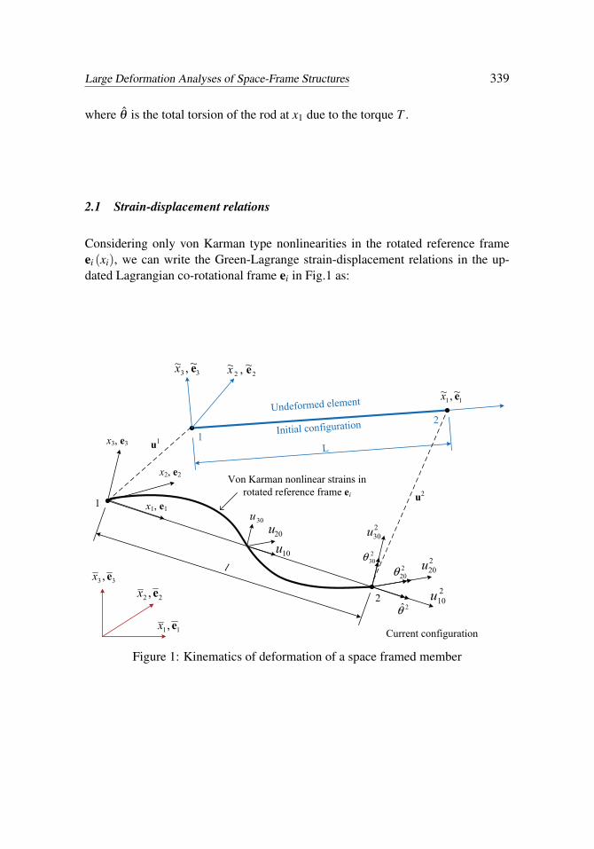
space, as shown in Fig.1. The current configuration of the rod, after arbitrarily largedeformations (but small strains) is also shown in Fig.1.

The local coordinates in the reference frame in the current configuration are xi andthe base vectors are ei (i = 1,2,3). The nodes 1 and 2 of the rod (or an element ofthe rod) are supposed to undergo arbitrarily large displacements, and the rotationsbetween the ei (i = 1,2,3) and the ek (k = 1,2,3) base vectors are assumed to bearbitrarily finite. In the continuing deformation from the current configuration, thelocal displacements in the xi (ei) coordinate system are assumed to be moderate,and the local gradient (∂u10/∂x1) is assumed to be small compared to the transverserotations (∂uα0/∂x1)(α = 2,3). Thus, in essence, a von-Karman type deformationis assumed for the continued deformation from the current configuration, in the co-rotational frame of reference ei (i = 1,2,3) in the local coordinates xi (i = 1,2,3).If H is the characteristic dimension of the cross-section of the rod, the preciseassumptions governing the continued deformations from the current configurationareu10

H� 1;

HL� 1

uα0

H≈ O(1)(α = 2,3)

∂u10

∂x1� ∂uα0

∂x1(α = 2,3)

and(

∂uα0∂x1

)2(α = 2,3) are not negligible.

As shown in Fig.2, we consider the large deformations of a cylindrical rod, sub-jected to bending (in two directions), and torsion around x1. The cross-section isunsymmetrical around x2 and x3 axes, and is constant along x1.

As shown in Fig.2, the warping displacement due to the torque T around x1 axis isu1T (x2,x3) and does not depend on x1, the axial displacement at the origin (x2 =x3 = 0) is u10 (x1), and the bending displacement at x2 = x3 = 0 along the axis x1are u20 (x1) (along x2) and u30 (x1) (along x3).

We consider only loading situations when the generally 3-dimensional displace-ment state in the ei system, donated as

ui = ui (xk) i = 1,2,3; k = 1,2,3

is simplified to be of the type:

u1 = u1T (x2,x3)+u10 (x1)− x2∂u20

∂x1− x3

∂u30

∂x1

u2 = u20 (x1)− θx3

u3 = u30 (x1)+ θx2

(1)


where θ is the total torsion of the rod at x1 due to the torque T .

2.1 Strain-displacement relations

Considering only von Karman type nonlinearities in the rotated reference frameei (xi), we can write the Green-Lagrange strain-displacement relations in the up-dated Lagrangian co-rotational frame ei in Fig.1 as:

x3, e3

1

2210u

220u

230u

2θ

220θ

230θ

11, ex

Von Karman nonlinear strains in rotated reference frame ei

12

11~,~ ex

Undeformed element

Initial configuration

Current configuration

10u

30u20u

x2, e2

x1, e1

22~,~ ex33

~,~ ex

22 , ex33 , ex

L

l

u1

u2

Figure 1: Kinematics of deformation of a space framed member


x1,e1T

M2

M3

x2

x3

x1

x2

x3

x1

u30(x1)u20(x1)

u10(x1)

u1T(x2,x3) due to T

θ

Current configuration

x2,e2

x3,e3

Figure 2: Large deformation analysis model of a cylindrical rod

ε11 =∂u1

∂x1+

12

(∂u2

∂x1

)2

+12

(∂u3

∂x1

)2

=∂u10

∂x1+

12

(∂u20

∂x1

)2

+12

(∂u30

∂x1

)2

− x2∂ 2u20

∂x21− x3

∂ 2u30

∂x21

ε12 =12

(∂u1

∂x2+

∂u2

∂x1

)=

12

(∂u1T

∂x2− ∂u20

∂x1+

∂u20

∂x1− ∂ θ

∂x1x3

)=

12

(∂u1T

∂x2−θ x3

)ε13 =

12

(∂u1

∂x3+

∂u3

∂x1

)=

12

(∂u1T

∂x3− ∂u30

∂x1+

∂u30

∂x1+θx2

)=

12

(∂u1T

∂x3+θx2

)ε22 =

∂u2

∂x2+

12

(∂u1

∂x2

)2

+12

(∂u2

∂x2

)2

+12

(∂u3

∂x2

)2

≈ 0+12

(∂u20

∂x1

)2

+0≈ 0

ε23 ≈ 0

ε33 ≈ 0

(2)


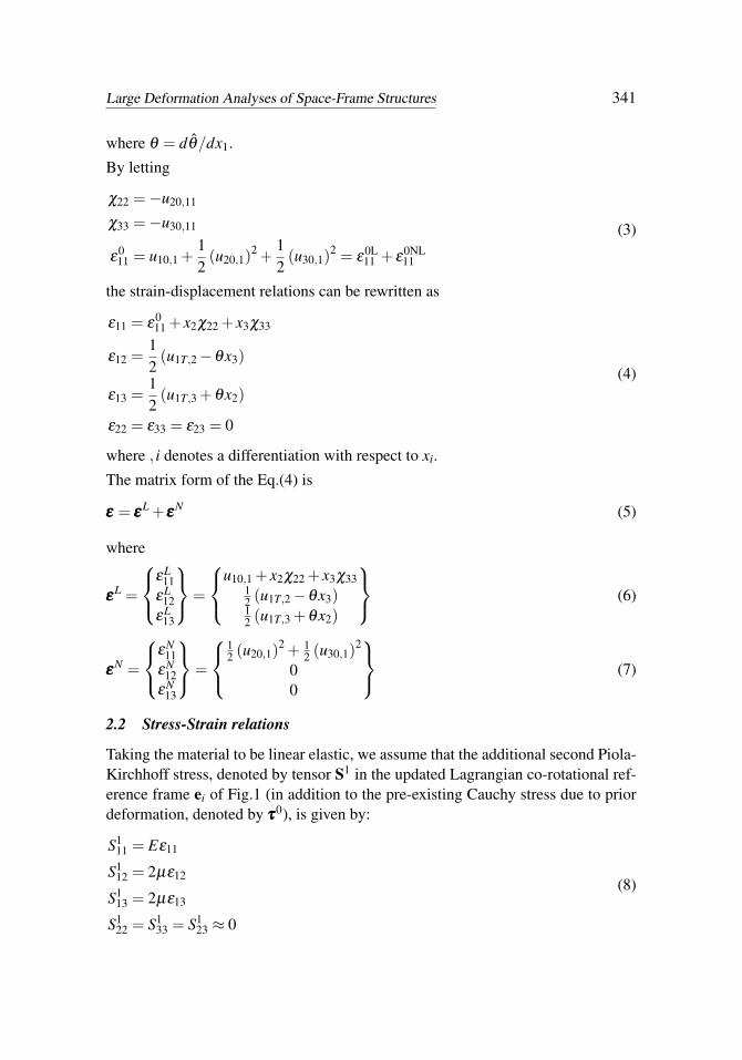
where θ = dθ/dx1.

By letting

χ22 =−u20,11

χ33 =−u30,11

ε011 = u10,1 +

12

(u20,1)2 +

12

(u30,1)2 = ε

0L11 + ε

0NL11

(3)

the strain-displacement relations can be rewritten as

ε11 = ε011 + x2χ22 + x3χ33

ε12 =12

(u1T,2−θx3)

ε13 =12

(u1T,3 +θx2)

ε22 = ε33 = ε23 = 0

(4)

where , i denotes a differentiation with respect to xi.

The matrix form of the Eq.(4) is

εεε = εεεL +εεε

N (5)

where

εεεL =

εL

11εL

12εL

13

=

u10,1 + x2χ22 + x3χ33

12 (u1T,2−θx3)12 (u1T,3 +θx2)

(6)

εεεN =

εN

11εN

12εN

13

=

12 (u20,1)

2 + 12 (u30,1)

2

00

(7)

2.2 Stress-Strain relations

Taking the material to be linear elastic, we assume that the additional second Piola-Kirchhoff stress, denoted by tensor S1 in the updated Lagrangian co-rotational ref-erence frame ei of Fig.1 (in addition to the pre-existing Cauchy stress due to priordeformation, denoted by τττ0), is given by:

S111 = Eε11

S112 = 2µε12

S113 = 2µε13

S122 = S1

33 = S123 ≈ 0

(8)


where µ = E2(1+ν) ; E is the elastic modulus; ν is the Poisson ratio.

By using Eq.(5), Eq.(8) can also be written as

S1 = D(εεε

L +εεεN)= S1L +S1N (9)

where

D =

E 0 00 2µ 00 0 2µ

(10)

From Eq.(4) and Eq.(8), the generalized nodal forces of the rod element in Fig.2can be written as

N11 =∫

AS1

11dA = E(

Aε011 + χ22

∫A

x2dA+ χ33

∫A

x3dA)

= E(Aε

011 + I2χ22 + I3χ33

)M33 =

∫A

S111x3dA = E

∫A

(Aε

011 + x2χ22 + x3χ33

)x3dA

= E(I3ε

011 + I23χ22 + I33χ33

)M22 =

∫A

S111x2dA = E

∫A

(Aε

011 + x2χ22 + x3χ33

)x2dA

= E(I2ε

011 + I22χ22 + I23χ33

)T =

∫A

S113x2−S1

12x3dA = 2µ

∫A(x2ε13 + x3ε12)x2dA

=2µ

2

∫A[(u1T,3 +θ x2)x2− (u1T,2−θx3)]dA

= µ

∫A

θ(x2

2 + x23)

dA+ µ

∫A(u1T,3x2−u1T,2x3)dA

= µIrrθ + µ

∮S(u1T n3x2−u1T n2x3)dS

= µIrrθ

(11)

where n j is the outward norm, I2 =∫

A x2dA, I3 =∫

A x3dA, I22 =∫

A x22dA, I33 =∫

A x23dA, I23 =

∫A x2x3dA, and Irr =

∫A

(x2

2 + x23)

dA.

The matrix form of the above equations isσ1σ2σ3σ4

=

N11M22M33T

=

EA EI2 EI3 0EI2 EI22 EI23 0EI3 EI23 EI33 00 0 0 µIrr

ε011

χ22χ33θ

(12)


It can be denoted as

σσσ = DE (13)

where

σσσ =

σ1σ2σ3σ4

=

N11M22M33T

= element generalized stresses (14)

D =

EA EI2 EI3 0EI2 EI22 EI23 0EI3 EI23 EI33 00 0 0 µIrr

(15)

E = EL +EN =

E1E2E3E4

=

ε0

11χ22χ33θ

= element generalized strains (16)

where

EL =[u10,1 −u20,11 −u30,11 θ,1

]T(17)

EN =[

12

(u2

20,1 +u230,1

)0 0 0

]T(18)

3 Updated Lagrangian formulation in the co-rotational reference frame ei

3.1 The use of the Reissner variational principle in the co-rotational updatedLagrangian reference frame

If τ0i j are the initial Cauchy stresses in the updated Lagrangian co-rotational frame

ei of Fig.1, S1i j are the additional (incremental) second Piola-Kirchhoff stresses in

the same updated Lagrangian co-rotational frame with axes ei, Si j = S1i j +τ0

i j are thetotal stresses, and ui are the incremental displacements in the co-rotational updated-Lagrangian reference frame, the functional of the Reissner variational principle(Reissner 1953) [see also Atluri and Reissner (1989)] for the incremental S1

i j and ui

in the co-rotational updated Lagrangian reference frame is given by [Atluri 1979,1980]

ΠR =∫V

{−B(S1

i j)+

12

τ0i juk,iuk, j +

12

Si j (ui, j +u j,i)−ρbiui

}dV −

∫Sσ

TiuidS (19)


Where V is the volume in the current co-rotational reference state, Sσ is the surfacewhere tractions are prescribed, bi = b0

i +b1i are the body forces per unit volume in

the current reference state, and Ti = T 0i + T 1

i are the given boundary tractions.

The conditions of stationarity of ΠR, with respect to variations δS1i j and δui lead

to the following incremental equations in the co-rotational updated- Lagrangianreference frame.

∂B∂S1

i j=

12

[ui, j +u j,i] (20)

[S1

i j + τ0iku j,k

], j

+ρb1i =−

(τ

0i j), j−ρb0

i (21)

n j[S1

i j + τ0iku j,k

]−T 1

i =−n jτ0i j + T 0

i at Sσ (22)

In Eq.(19), the displacement boundary conditions,

ui = ui at Su (23)

are assumed to be satisfied a priori, at the external boundary, Su. Eq.(21) leads toequilibrium correction iterations.

If the variational principle embodied in Eq.(19) is applied to a group of finite ele-ments, Vm, m = 1,2, · · · ,N, which comprise the volume V , ie, V = ∑Vm, then

ΠR =

∑m

∫Vm

{−B(S1

i j)+

12

τ0i juk, juk, j +

12

Si j (ui, j +u j,i)−ρbiui

}dV −

∫Sσm

TiuidS

(24)

Let ∂Vm be the boundary of Vm, and ρm be the part of ∂Vm which is shared by theelement with its neighbouring elements. If the trial function ui and the test function∂ui in each Vm are such that the inter-element continuity condition,

u+i = u−i at ρm (25)

(where + and – refer to either side of the boundary ρm) is satisfied a priori, then itcan be shown (Atluri 1975,1984; Atluri and Murakawa 1977; Atluri, Gallagher andZienkiewicz 1983) that the conditions of stationarity of ΠR in Eq.(24) lead to:

∂B∂S1

i j=

12[ui, j +u j,i

]in Vm (26)


[S1

i j + τ0iku j,k

], j

+ρb1i =−τ

0i j, j−ρb0

i in Vm (27)

[ni(S1

i j + τ0iku j,k

)]++[ni(S1

i j + τ0iku j,k

)]−=−

[niτ

0i j]+− [niτ

0i j]−

at ρm (28)

n j[S1

i j + τ0iku j,k

]− T 1

i =−n jτ0i j + T 0

i at Sσm (29)

Eq.(28) is the condition of traction reciprocity at the inter-element boundary, ρm.Eqs(27) and (28) lead to corrective iterations for equilibrium within each element,and traction reciprocity at the inter-element boundaries, respectively.

Carrying out the integration over the cross sectional area of each rod, and usingEqs.(4) and (12), Eq.(24) can be easily shown to reduce to:

ΠR = ∑elem

∫l

(−1

2σσσ

T D−1σσσ

)dl +

∫l

N011

12(u2

20,1 +u230,1)

dl

+∫l

(N11ε

0L11 + M22χ22 + M33χ33 + T θ

)dl− Qq

(30)

where D is given in Eq.(15), C = D−1, l is the length of the rod element, σσσ is givenin Eq.(14), σ0

i j =[N0

11 M022 M0

33 T 0]T is the initial element-generalized- stress

in the corotational reference coordinates ei, and σσσ =σσσ0 +σσσ =[N11 M22 M33 T

]Tis the total element generalized stresses in the corotational reference coordinates ei.Q is the nodal external generalized force vector (consisting of force as well asmoments) in the global Cartesian reference frame, and q is the incremental nodalgeneralized displacement vector (consisting of displacements as well as rotations)in the global Cartesian reference frame. It should be noted that while ΠR in Eq.(30)represents a sum over the elements, the relevant integrals are evaluated over eachelement in it’s own co-rotational updated Lagrangian reference frame.


By integrating by parts, the second item of the left side can be written as

∫l

N11ε0L11 dl =

∫l

N11u10,1dl =−∫l

N11,1u10dl + N11u10∣∣l0∫

l

M22χ22dl =−∫l

M22u20,11dl

=−∫l

M22,11u20dl + M22,1u20∣∣l0− M22u20,1

∣∣l0∫

l

M33χ33dl =−∫l

M33u30,11dl

=−∫l

M33,11u30dl + M33,1u30∣∣l0− M33u30,1

∣∣l0∫

l

T θdl =∫l

T θ,1dl =−∫l

T,1θdl + T θ∣∣l0

(31)

The condition of stationarity of ΠR in Eq.(30) leads to:

D−1σ = E =

[u10,1 −u20,11 −u30,11 θ

]TN11,1 = 0 in each element

T,1 = 0 in each element

M22,11 +(N0

11u20,1),1 = 0 in each element

M33,11 +(N0

11u30,1),1 = 0 in each element

(32)

and the nodal equilibrium equations, which arise out of the term:

∑elem

(N11δu10

∣∣l0 + M22,1δu20

∣∣l0 − M22δu20,1

∣∣l0 + M33,1δu30

∣∣l0 − M33δu30,1

∣∣l0 +

T δ θ∣∣l0 +(N0

11u20,1)

δ u20|l0 +(N0

11u30,1)

δ u30|l0− Qδq)

= 0

(33)


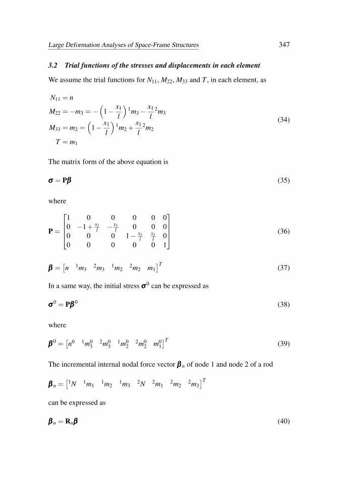
3.2 Trial functions of the stresses and displacements in each element

We assume the trial functions for N11, M22, M33 and T , in each element, as

N11 = n

M22 =−m3 =−(

1− x1

l

)1m3−

x1

l2m3

M33 = m2 =(

1− x1

l

)1m2 +

x1

l2m2

T = m1

(34)

The matrix form of the above equation is

σσσ = Pβββ (35)

where

P =

1 0 0 0 0 00 −1+ x1

l − x1l 0 0 0

0 0 0 1− x1l

x1l 0

0 0 0 0 0 1

(36)

βββ =[n 1m3

2m31m2

2m2 m1]T (37)

In a same way, the initial stress σσσ0 can be expressed as

σσσ0 = Pβββ

0 (38)

where

βββ0 =

[n0 1m0

32m0

31m0

22m0

2 m01

]T (39)

The incremental internal nodal force vector βββ n of node 1 and node 2 of a rod

βββ n =[

1N 1m11m2

1m32N 2m1

2m22m3]T

can be expressed as

βββ n = Rnβββ (40)


where

Rn =

1 0 0 0 0 00 0 0 0 0 10 0 0 1 0 00 1 0 0 0 01 0 0 0 0 00 0 0 0 0 10 0 0 0 1 00 0 1 0 0 0

(41)

In the functional in Eq.(30), only the squares of (u20,1) and (u30,1) occur withineach element. Thus, (u20,1) and (u30,1) are assumed directly to be linear withineach element, in terms of their respective nodal values. This will be enormouslysimple and advantageous in the case of plate and shell elements. This is in contrastto the primal (displacement) approach (Cai, Paik and Atluri 2010) wherein u20 andu30 were required to be C1 continuous over each element, and thus were assumed tobe Herimitian polynomials over each element. In this paper, however, we assume:

uθ = Nθ aθ =[

φ1 0 φ2 00 φ1 0 φ2

]1θ201θ302θ202θ30

(42)

whereφ1 = 1−ξ

φ2 = ξ

(ξ =

x1

l

)(43)

Assuming that ‘a’ represents the vector of generalized displacements of the nodesof the rod element in the updated Lagrangian co-rotational frame ei of Fig.1, thedisplacement vectors of node i are:ia =

[iu1

iu2iu3

iu4iu5

iu6]T

=[

iu10iu20

iu30iθ iθ20

iθ30]T (i = 1,2)

(44)

The relation between aθ and a can be expressed as

aθ = Tθ a (45)

where

Tθ =

0 0 0 0 1 0 0 0 0 0 0 00 0 0 0 0 1 0 0 0 0 0 00 0 0 0 0 0 0 0 0 0 1 00 0 0 0 0 0 0 0 0 0 0 1

(46)


3.3 Explicit expressions of the tangent stiffness matrix for each element

Because of the assumption of the trial functions of the stresses in Eqs.(35), thefollowing items in Eq.(31) become∫l

N11,1u10dl = 0

∫l

M22,11u20dl = 0

∫l

M33,11u30dl = 0

∫l

T,1θdl = 0

(47)

Eq.(30) can be rewritten as

ΠR =−ΠR1 +ΠR2 +ΠR3−ΠR4 (48)

where

ΠR1 = ∑elem

∫l

(12

σσσT D−1

σσσ

)dl = ∑

elem

∫l

(12

βββT PT CPβββ

)dl (49)

ΠR2 = ∑elem

{2N2u10− 1N1u10 +

1l

(1m3− 2m3)(2u20− 1u20

)+ 2m3

2θ30− 1m3

1θ30

+1l

(2m2− 1m2)(2u30− 1u30

)+ 2m2

2θ20− 1m2

1θ20 + 2m1

2θ − 1m1

1θ

}= ∑

elem

{(βββ n)

T Rσ a}

= ∑elem

{(βββ )T RT

n Rσ a}

(50)

where

Rσ =

−1 0 0 0 0 0 0 0 0 0 0 00 0 0 −1 0 0 0 0 0 0 0 00 0 1

l 0 −1 0 0 0 −1l 0 0 0

0 −1l 0 0 0 −1 0 1

l 0 0 0 00 0 0 0 0 0 1 0 0 0 0 00 0 0 0 0 0 0 0 0 1 0 00 0 −1

l 0 0 0 0 0 1l 0 1 0

0 1l 0 0 0 0 0 −1

l 0 0 0 1

(51)


ΠR3 = ∑elem

∫l

N011

[12

(u20,1)2 +

12

(u30,1)2]

dl = ∑elem

∫l

σ01

[12

(θ20)2 +

12

(θ30)2]

dl

= ∑elem

∫l

σ01

2uT

θ uθ dl = ∑elem

∫l

σ01

2aT TT

θ NTθ Nθ Tθ adl

(52)

Letting Ann = TTθ

NTθ

Nθ Tθ , ΠR3 can be rewritten as

ΠR3 = ∑elem

∫l

σ01

2aT Annadl (53)

and

ΠR4 = ∑elem

(aT F−aT RT

σ Rnβββ0) (54)

By invoking δΠR = 0, we can obtain

δΠR = ∑elem

δβββT

−∫l

PT CPβdl +RTn Rσ a

+

∑elem

δaT

RTσ Rnβββ +σ

01

∫l

Annadl +RTσ Rnβββ

0−F

(55)

Let

H =∫l

PT CPdl, G = RTn Rσ , KN = σ

01

∫l

Anndl, F0 = GTβββ

0 (56)

then

δΠR = ∑elem

δβββT {−Hβ +Ga}− ∑

elemδaT {GT

βββ +KNa−F+F0}= 0 (57)

Since δβββ T in Eq.(53) are independent and arbitrary in each element, one obtains

βββ = H−1Ga (58)

and

∑elem

δaT {(KL +KN)a−F+F0}= 0 (59)


where

KL = GTH - 1G (60)

KN = σ01

∫l

Anndl (61)

The components of the element tangent stiffness matrix, KL and KN , respectively,can be derived explicitly, after some simple algebra, as follows.

KN =lσ0

16

0 0 0 0 0 0 0 0 0 0 0 00 0 0 0 0 0 0 0 0 0 0

0 0 0 0 0 0 0 0 0 00 0 0 0 0 0 0 0 0

2 0 0 0 0 0 1 02 0 0 0 0 0 1

0 0 0 0 0 00 0 0 0 0

sym. 0 0 0 00 0 0

2 02

(62)

KL =ElA

[KL1 KL12KT

L12 KL2

](63)

where

KL1 =

A2 0 0 0 AI3 −AI212(AI22−I2

2)l2

12(AI23−I2I3)l2 0 −6(AI23−I2I3)

l6(AI22−I2

2)l

12(AI33−I23)

l2 0−6(AI33−I2

3)l

6(AI23−I2I3)l

Aµ

E Irr 0 0symmetric 4AI33−3I2

3 −4AI23 +3I2I34AI22−3I2

2

(64)


KL2 =

A2 0 0 0 AI3 −AI212(AI22−I2

2)l2

12(AI23−I2I3)l2 0 6(AI23−I2I3)

l−6(AI22−I2

2)l

12(AI33−I23)

l2 06(AI33−I2

3)l

−6(AI23−I2I3)l

Aµ

E Irr 0 0symmetric 4AI33−3I2

3 −4AI23 +3I2I34AI22−3I2

2

(65)

KL12 =

−A2 0 0 0 −AI3 AI2

0−12(AI22−I2

2)l2

−12(AI23−I2I3)l2 0 −6(AI23−I2I3)

l6(AI22−I2

2)l

0 −12(AI23−I2I3)l2

−12(AI33−I23)

l2 0−6(AI33−I2

3)l

6(AI23−I2I3)l

0 0 0 −Aµ

E Irr 0 0

−AI36(AI23−I2I3)

l6(AI33−I2

3)l 0 2AI33−3I2

3 −2AI23 +3I2I3

AI2−6(AI22−I2

2)l

−6(AI23−I2I3)l 0 −2AI23 +3I2I3 2AI22−3I2

2

(66)

Thus, KL is the usual linear symmetric (12×12) stiffness matrix of the beam in theco-rotational reference frame, with the geometric parameters I2, I3, I22, I33, I23 andIrr, and the current length l.

It is clear from the above procedures, that the present (12×12) symmetric tan-gent stiffness matrices of the beam in the co-rotational reference frame, based onthe Reissner variational principle and simplified rod theory, are much simpler thanthose of Kondon, Tanaka and Atluri (1986), Kondoh and Atluri (1987), and Shi andAtluri (1988). Moreover, the explicit expressions for the tangent stiffness matrix ofeach rod can be seen to be derived as text-book examples of nonlinear analyses.

3.4 Cubic trial functions of the displacements in the beam element, using theReissner variational principle

When using the Reissner functional in Eq.(30), one may directly assume the ro-tation field (u20,1) and (u30,1) as linear functions in terms only of their respectivenodal values, as in Eq.(42). Alternatively, u20 and u30 may be assumed as cubicpolynomials in terms of the four nodal values 1u20, 2u20, 1u20,1, 2u20,1 (1u30, 2u30,1u30,1, 2u30,1 for u30), and derive the element fields for u20,1 (and u30,1) from thesecubic polynomials [even though the Reissner principle does not demand it]. Thiswill be particularly advantageous for plate and shell elements which demand C1


continuity while using the potential energy approach, while C1 continuity of thedisplacement field will not be demanded in the Reissner principle.

In general, we assume over each element:

u20 = α1 +α2ξ +α3ξ2 +α4ξ

3

u30 = γ1 + γ2ξ + γ3ξ2 + γ4ξ

3 (67)

By letting

u20|ξ=ξ0= 1u20, u20|ξ=ξ1

= 2u20, u20,1|ξ=ξ0= 1

θ30, u20,1|ξ=ξ1= 2

θ30

u30|ξ=ξ0= 1u30, u30|ξ=ξ1

= 2u30,−u30,1|ξ=ξ0= 1

θ20,−u30,1|ξ=ξ1= 2

θ20(68)

we can approximate the displacement function in each rod element by

uc = Na =[

1N 2N]{1a

2a

}(69)

where

uc =[u10 u20 u30 θ

]T(70)

1N =

φ1 0 0 0 0 00 N1 0 0 0 N20 0 N1 0 −N2 00 0 0 φ1 0 0

(71)

1N =

φ2 0 0 0 0 00 N3 0 0 0 N40 0 N3 0 −N4 00 0 0 φ2 0 0

(72)

N1 = 1−3ξ2 +2ξ

3,N3 = 3ξ2−2ξ

3

N2 =(ξ −2ξ

2 +ξ3) l,N4 =

(ξ

3−ξ2) l

(73)

and φ1, φ2 are defined in Eq.(43).

By using the cubic trial functions of Eq.(69) and deriving the equations in a sameway as the section 3.3, we obtain the respective discrete equations, as follows.

∑elem

δaT {(KL +KcN)a−F+F0}= 0 (74)


where KL,F and F0 are the same as Eq.(59), and the nonlinear stiffness matrix KcN

is explicitly expressed as

(12×12 symmetric matrix)

KcN =

σ01l

0 0 0 0 0 0 0 0 0 0 0 01.2 0 0 0 0.1l 0 −1.2 0 0 0 0.1l

1.2 0 −0.1l 0 0 0 −1.2 0 −0.1l 00 0 0 0 0 0 0 0 0

2l2

15 0 0 0 0.1l 0 −l2

30 02l2

15 0 −0.1l 0 0 0 −l2

300 0 0 0 0 0

1.2 0 0 0 −0.1lsym. 1.2 0 0.1l 0

0 0 02l2

15 02l2

15

(75)

4 Transformation between deformation dependent co-rotational local [ei],and the global [ei] frames of reference

As shown in Fig.1, xi (i = 1,2,3) are the global coordinates with unit basis vectorsei. xi and ei are the local coordinates for the rod element at the undeformed element.The basis vector ei are initially chosen such that (Shi and Atluri 1988, Cai, Paik andAtluri 2010)

e1 = (∆x1e1 +∆x2e2 +∆x3e3)/L

e2 = (e3× e1)/|e3× e1|e3 = e1× e2

(76)

where ∆xi = x2i − x1

i ,L =(∆x2

1 +∆x22 +∆x2

3) 1

2 .

Then ei and ei have the following relations:e1e2e3

=

∆x1/L ∆x2/L ∆x3/L−∆x2/S ∆x1/S 0

−∆x1∆x3/(SL) −∆x2∆x3/(SL) s/L

e1e2e3

(77)

where S =(∆x2

1 +∆x22) 1

2 .


Thus we can define a transformation matrix λλλ 0 between ei and ei as

λλλ 0 =

∆x1/L ∆x2/L ∆x3/L−∆x2/S ∆x1/S 0

−∆x1∆x3/(SL) −∆x2∆x3/(SL) S/L

(78)

When the element is parallel to the x3 axis, S =[∆x2

1 +∆x22] 1

2 = 0 and Eq.(64) isnot valid. In this case, the local coordinates is determined by

e1 = e3, e2 = e2, e3 =−e1 (79)

Let xi and ei be the co-rotational reference coordinates for the deformed rod ele-ment. In order to continuously define the local coordinates of the same rod elementduring the whole range of large deformation, the basis vectors ei are chosen suchthat

e1 = (∆x1e1 +∆x2e2 +∆x3e3)/l = a1e1 +a2e2 +a3e3

e2 = (e3× e1)/|e3× e1|e3 = e1× e2

(80)

where ∆xi = x2i − x1

i , l =(∆x2

1 +∆x22 +∆x2

3) 1

2 .

We denote e3 in Eq.(77) as

e3 = c1e1 + c2e2 + c3e3 (81)

Then ei and ei have the following relations:e1e2e3

=

a1 a2 a3b1 b2 b3

a2b3−a3b2 a3b1−a1b3 a1b2−a2b1

e1e2e3

= λλλ 0ei (82)

where

b1 = (c2a3− c3a2)/l31

b2 = (c3a1− c1a3)/l31

b3 = (c1a2− c2a1)/l31

(83)

l31 =[(c2a3− c3a2)

2 +(c3a1− c1a3)2 +(c1a2− c2a1)

2] 1

2(84)


and

λλλ 0 =

a1 a2 a3b1 b2 b3

a2b3−a3b2 a3b1−a1b3 a1b2−a2b1

(85)

Thus, the transformation matrix λλλ , between the 12 generalized coordinates in theco-rotational reference frame, and the corresponding 12 coordinates in the globalCartesian reference frame, is given by

λλλ =

λλλ 0

λλλ 0λλλ 0

λλλ 0

(86)

Letting xi and ei be the reference coordinates, and repeating the above steps [Eq.(70)– Eq.(86)], the transformation matrix of each incremental step can be obtained in asame way.

Then the element matrices are transformed to the global coordinate system using

a = λλλT a (87)

K = λλλT Kλλλ (88)

F = λλλT F (89)

where a, K, F are respectively the generalized nodal displacements, element tan-gent stiffness matrix and generalized nodal forces, in the global coordinates system.

The Newton-Raphson method, modified Newton-Rapson method or the artificialtime integration method (Liu 2007a, 2007b; Liu and Atluri 2008) can be employedto solve Eqs.(59) and (74). In this implementation, the Newton-Raphson algorithmis used. In all examples, the assumptions of linear trial functions of the rotationswere employed, except where stated otherwise.

5 Numerical examples

5.1 Buckling of a beam

The (12×12) tangent stiffness matrix for a beam in space should be capable ofpredicting buckling under compressive axial loads, when such an axial load inter-acts with the transverse displacement in the beam. We consider a simply supportedbeam subject to an axial force as shown in Fig.3 and assume that EI = 1 and L = 1.


The buckling loads of the beam obtained by the present method using differentnumbers of elements are shown in Tab.1. It is seen that the buckling load predictedby the present method agrees well with the analytical solution (buckling load isπ2).

Figure 3: A simply supported beam subject to an axial force

Table 1: Buckling load of the simply supported beam

Present method(Number of elements) Analytical1 2 3 4 10 solution

Buckling load 12.005 12.005 10.799 10.384 9.950 9.870

When the beam is fixed at x1 = 0, while at the other end it is free and under acompressive load P, the buckling load of the beam obtained by the present methodusing different number of elements is shown in Tab.2 (the analytical solution isπ2EI4L2 ).

Table 2: Buckling load of the beam fixed at x1 = 0

Present method(Number of elements) Analytical1 2 3 4 10 solution

Buckling load 3.0003 2.5967 2.5240 2.4994 2.4722 2.4674

5.2 Large deformation analysis of a cantilever beam with a symmetric crosssection

A large deflection and moderate rotation analysis of a cantilever beam subject to atransverse load at the tip, as shown in Fig. 5, is considered. The cross section ofthe beam is a square with h = 1. The Poisson’s ration is ν = 0.3. Fig.5 shows theresults obtained in the analysis of the cantilever problem. It is seen that the presentresults using 10 elements agree well with those of Bathe and Bolourchi (1979).


Figure 4: A cantilever beam subject to a transverse load at the tip

PL2 / E

I

L/δ

Figure 5: Deflections of a cantilever under a concentrated load


5.3 Large rotations of a cantilever subject to an end-moment and a transverseload

An initially-straight cantilever subject to an end moment M∗ = ML2πEI (Crisfield

1990) as shown in Fig.6, is considered. The beam is divided into 10 equal ele-ments. When M∗ = 1, the beam is curled into a complete circle as shown in Fig.6.

If a non-conservative, follower-type transverse load P∗ = PL2

2πEI is applied at the tip,instead of M∗, the initial and deformed geometries of the cantilever are shown inFig.7.

5.4 Large deformation analysis of a cantilever beam with an asymmetric crosssection

We consider the large deflection of a cantilever beam with an asymmetric crosssection, as shown in Fig.8. The Poisson’s ration is ν = 0.3. The areas of thesymmetric and asymmetric cross section in Fig.8 are all equal to 1.

Fig.9 shows the comparison of the deflections in x3 direction, between the casesof symmetric and asymmetric cross sections. Fig.10 shows the deflection in x2direction for the cantilever beam with an asymmetric cross section. However, thedeflections in x2 direction are zero in the case of a symmetric cross section.

5.5 Large displacement analysis of a 45-degree space bend

The large displacement response of a 45-degree bend subject to a concentrated endload [Bathe and Bolourchi (1979)] is calculated as shown in Fig.11. The radiusof the bend is 100, the cross section area is 1 and lies in the x1− x2 plane. Theconcentrated is applied in the x3 direction.

8 equal straight elements and 140 equal load steps are used in the analysis of theproblem. Fig.12 shows the tip deflection predicted by the present method and Batheand Bolourchi (1979). It can be seen that the results of the present method agreeexcellently with the results of Bathe and Bolourchi (1979).

5.6 A framed dome

A framed dome shown in Fig.13 is considered (Shi and Atluri 1988). A concen-trated vertical load P is applied at the crown point. Each member of the dome ismodeled by 4 elements.

The linear approaches of the displacements in Eq.(42) are robust for most casesin the large deformation analysis of the space frames. However, the solution wasfound to diverge when λ > 0.59 by using the linear interpolations for rotations


L

EI2MLM*

π=

M*=0

M*=0.3M*=0.5

M*=1.0

Figure 6: Initial and deformed geometries for cantilever subject to an end-moment

L

EI2PLP

2*

π=

P*=0.0

P*=1.0

P*=2.0

P*=4.0

P*=6.0

Figure 7: Initial and deformed geometries for cantilever subject to a transverse load


L=50

EI

P

δ

x1

x2

x3

bb

a(a=0.2, b=1.3)

P

Asymmetric cross section

x2

x3

bbP

a

Symmetric cross section

(a=0.2, b=5/6)

x2

x3

Figure 8: A cantilever beam with an asymmetric cross section

for this example. Thus, the nonlinear stiffness matrix in Eq.(75), which is derivedfrom cubic trial functions of the displacements, was used, and the converged resultsshown in Fig.14 were obtained.

6 Conclusions

Based on the Reissner variational principle and a von Karman type nonlinear theoryin a rotated reference frame, a simplified finite deformation theory of a cylindricalrod subjected to bending and torsion has been developed. The present (12×12)symmetric explicit tangent stiffness matrices of the beam are much simpler thanthose of many others based on the primal approach or potential energy approach.


L/δ

Figure 9: Comparison of the deflections in x3 direction of a cantilever beam

Lu 2

Figure 10: Deflections in x2 direction for the cantilever beam with asymmetriccross section

The explicit expressions for the tangent stiffness matrix of each element can beseen to be derived as text-book examples of nonlinear analyses. The proposedmethod is capable of handling large rotation geometrically nonlinear analysis offrames with arbitrary cross sections, which haven’t been considered by a majorityof previous studies. Numerical examples demonstrate that the present method isjust as competitive as the existing methods in terms of accuracy and efficiency.


Figure 11: Model of a 45-degree circular bend

0 1 2 3 4 5 6 70.0

0.1

0.2

0.3

0.4

0.5

0.6

Non

-dim

ensi

onal

tip

defle

ctio

n

Load parameter

Present method

Bathe,Bolourchi(1979)

Linear solutionu3/R

-u2/R

-u1/R

EIPRk

2

=

u3/R

Figure 12: Three-dimensional large deformation of a 45-degree circular bend


1.55

4.55

1.22

10.885

21.115

Figure 13: Framed dome (the unit of length is metre)

The present method can be extended to consider the formation of plastic hinges ineach beam of the frame; and also to consider large-rotations of plates and shells,by implementing only a von Karman type nonlinear theory in the co-rotationalreference frame of each beam/plate element. It is noted that the present approachdoes not involve any reduced integration, or suppression of Kinematic modes.

Acknowledgement: The authors gratefully acknowledge the support of the Na-ture Science Foundation of China (NSFC, 10972161). This research was alsosupported by the World Class University (WCU) program through the NationalResearch Foundation of Korea funded by the Ministry of Education, Science andTechnology (Grant no.: R33-10049). The second author is also pleased to acknowl-edge the support of the Lloyd’s Register Educational Trust (LRET) which is anindependent charity working to achieve advances in transportation, science, engi-


0.0 0.5 1.0 1.5 2.0 2.50.0

0.2

0.4

0.6

0.8

Present method

Kondoh,Tanaka,Atluri(1986)

Shi,Atluri(1988)

MN8.123λP ×=

crP/Pλ =

d(m)

Figure 14: Force-displacement curve for the crown point of a framed dome

neering and technology education, training and research worldwide for the benefitof all.

References

Atluri, S.N. (1975): On ’hybrid’ finite element models in solid mechanics, Ad-vances in computer methods for partial differential equations, R. Vichrevetsky, Ed.,AICA, pp. 346-355.

Atluri, S.N. (1979): On rate principles for finite strain analysis of elastic and inelas-tic nonlinear solids, Recent research on mechanical behavior, University of TokyoPress, pp. 79-107.

Atluri, S.N. (1980): On some new general and complementary energy theoremsfor the rate problems in finite strain, classical elastoplasticity. Journal of StructuralMechanics, Vol. 8(1), pp. 61-92.

Atluri, S.N. (1984): Alternate stress and conjugate strain measures, and mixedvariational formulations involving rigid rotations, for computational analyses offinitely deformed plates and shells: part-I: thoery. Computers & Structures, Vol.18(1), pp. 93-116.


Atluri, S.N.; Cazzani, A. (1994): Rotations in computational solid mechanics,invited feature article. Archives for Computational Methods in Engg., ICNME,Barcelona, Spain, Vol 2(1), pp. 49-138.

Atluri, S. N.; Gallagher, R. H.; Zienkiewicz, O. C. (Editors). (1983): Hybrid &Mixed Finite Element Methods, J. Wiley & Sons, 600 pages.

Atluri, S.N.; Iura, M.; Vasudevan, S.(2001): A consistent theory of finite stretchesand finite rotations, in space-curved beams of arbitrary cross-section. Computa-tional Mechanics, vol.27, pp.271-281

Atluri, S.N.; Murakawa, H. (1977): On hybrid finite element models in nonlinearsolid mechanics, finite elements in nonlinear mechanics, P.G. Bergan et al, Eds.,Tapir Press, Norway, vol. 1, pp. 3-40.

Atluri, S.N.; Reissner, E. (1989): On the formulation of variational theorems in-volving volume constraints. Computational Mechanics, vol. 5, pp 337-344.

Auricchio, F.; Carotenuto, P.; Reali, A. (2008): On the geometrically exact beammodel: A consistent, effective and simple derivation from three-dimensional finite-elasticity. International Journal of Solids and Structures, vol.45, pp. 4766–4781.

Bathe, K.J.; Bolourchi, S. (1979): Large displacement analysis of three- dimen-sional beam structures. International Journal for Numerical Methods in Engineer-ing, vol.14, pp.961-986.

Cai, Y.C.; Paik, J.K.; Atluri S.N. (2010): Large deformation analyses of space-frame structures, with members of arbitrary cross-section, using explicit tangentstiffness matrices, based on a von Karman type nonlinear theory in rotated referenceframes. CMES: Computer Modeling in Engineering & Sciences, vol. 53, no. 2, pp.123-152.

Chan, S.L. (1996): Large deflection dynamic analysis of space frames. Computers& Structures, vol. 58, pp.381-387.

Crisfield, M.A. (1990): A consistent co-rotational formulation for non-linear, three-dimensional, beam-elements. Computer Methods in Applied Mechanics and Engi-neering, vol.81, pp. 131–150.

Dinis, L.W.J.S.; Jorge, R.M.N.; Belinha, J. (2009): Large deformation applica-tions with the radial natural neighbours interpolators. CMES: Computer Modelingin Engineering & Sciences, vol.44, pp. 1-34

Gendy, A.S.; Saleeb, A.F. (1992): On the finite element analysis of the spatialresponse of curved beams with arbitrary thin-walled sections. Computers & Struc-tures, vol.44, pp.639-652

Han, Z.D.; Rajendran, A.M.; Atluri, S.N. (2005): Meshless Local Petrov- Galerkin(MLPG) approaches for solving nonlinear problems with large deformations and


rotations. CMES: Computer Modeling in Engineering & Sciences, vol.10, pp. 1-12

Iura, M.; Atluri, S.N. (1988): Dynamic analysis of finitely stretched and rotated3-dimensional space-curved beams. Computers & Structures, Vol. 29, pp.875-889

Izzuddin, B.A. (2001): Conceptual issues in geometrically nonlinear analysis of3D framed structures. Computer Methods in Applied Mechanics and Engineering,vol.191, pp. 1029–1053.

Kondoh, K.; Tanaka, K.; Atluri, S.N. (1986): An explict expression for thetangent-stiffness of a finitely deformed 3-D beam and its use in the analysis ofspace frames. Computers & Structures, vol.24, pp.253-271.

Kondoh, K.; Atluri, S.N. (1987): Large-deformation, elasto-plastic analysis offrames under nonconservative loading, using explicitly derived tangent stiffnessesbased on assumed stresses. Computational Mechanics, vol.2, pp.1-25.

Lee, M.H.; Chen, W.H. (2009): A three-dimensional meshless scheme with back-ground grid for electrostatic-structural analysis. CMC: Computers Materials &Continua, vol.11, pp. 59-77

Lee, S.Y.; Lin, S.M.; Lee, C.S.; Lu, S.Y.; Liu, Y.T. (2008): Exact large deflec-tion of beams with nonlinear boundary conditions.CMES: Computer Modeling inEngineering & Sciences, vol.30, pp. 27-36

Lee, S.Y.; Lu, S.Y.; Liu, Y.R.; Huang, H.C. (2008): Exact large deflection so-lutions for Timoshenko beams with nonlinear boundary conditions. CMES: Com-puter Modeling in Engineering & Sciences, vol.33, pp. 293-312

Lee, S.Y.; Wu, J.S. (2009): Exact Solutions for the Free Vibration of ExtensionalCurved Non-uniform Timoshenko Beams. CMES: Computer Modeling in Engi-neering & Sciences,vol.40, pp.133-154.

Liu, C. S. (2007a): A modified Trefftz method for two-dimensional Laplace equa-tion considering the domain’s characteristic length. CMES: Computer Modeling inEngineering & Sciences, vol. 21, pp. 53-66.

Liu, C.S. (2007b): A highly accurate solver for the mixed-boundary potential prob-lem and singular problem in arbitrary plane domain. CMES: Computer Modelingin Engineering & Sciences, vol. 20, pp. 111-122.

Liu, C.S.; Atluri, S.N. (2008): A novel time integration method for solving a largesystem of non-linear algebraic equations. CMES: Computer Modeling in Engineer-ing & Sciences, vol.31, pp. 71-83.

Lo, S.H. (1992): Geometrically nonlinear formulation of 3D finite strain beamelement with large rotations. Computers & Structures, vol.44, pp.147-157

Mata, P.; Oller, S.; Barbat A.H. (2007): Static analysis of beam structures un-der nonlinear geometric and constitutive behavior. Computer Methods in Applied


Mechanics and Engineering, vol.196, pp. 4458–4478.

Mata, P.; Oller, S.; Barbat A.H. (2008): Dynamic analysis of beam structuresconsidering geometric and constitutive nonlinearity. Computer Methods in AppliedMechanics and Engineering, vol.197, pp. 857–878.

Punch, E.F.; Atluri, S.N. (1984): Development and testing of stable, invariant,isoparametric curvilinear 2-D and 3-D hybrid-stress elements. Computer Methodsin Applied Mechanics and Engineering, Vol.47, pp.331-356

Rabczuk, T.; Areias, P. (2006): A meshfree thin shell for arbitrary evolving cracksbased on an extrinsic basis. CMES: Computer Modeling in Engineering & Sci-ences,vol.16, pp.115-130.

Reissner, E. (1953): On a variational theorem for finite elastic deformations, Jour-nal of Mathematics & Physics, vol. 32, pp. 129-135.

Shaw, A.; Roy, D. (2007): A novel form of reproducing kernel interpolationmethod with applications to nonlinear mechanics. CMES: Computer Modeling inEngineering & Sciences,vol.19, pp.69-98.

Simo, J.C. (1985): A finite strain beam formulation. The three-dimensional dy-namic problem. Part I. Computer Methods in Applied Mechanics and Engineering,vol. 49, pp.55–70.

Shi, G.; Atluri, S.N. (1988): Elasto-plastic large deformation analysis of space-frames: a plastic-hinge and strss-based explict derivation of tangent stiffnesses.International Journal for Numerical Methods in Engineering, vol.26, pp.589-615.

Wen, P.H.; Hon, Y.C. (2007): Geometrically nonlinear analysis of Reissner- Mindlinplate by meshless computation. CMES: Computer Modeling in Engineering & Sci-ences, vol.21, pp.177-191.

Wu, T.Y.; Tsai, W.G.;Lee, J.J. (2009):Dynamic elastic-plastic and large deflec-tion analyses of frame structures using motion analysis of structures. Thin-WalledStructures, vol.47, pp. 1177-1190.

Xue, Q.; Meek J.L. (2001): Dynamic response and instablity of frame structures.Computer Methods in Applied Mechanics and Engineering, vol.190, pp. 5233–5242.

Zhou, Z.H.; Chan,S.L. (2004a): Elastoplastic and Large Deflection Analysis ofSteel Frames by One Element per Member. I: One Hinge along Member. Journalof Structural Engineering, vol. 130, pp.538–544.

Zhou, Z.H.; Chan,S.L. (2004b): Elastoplastic and Large Deflection Analysis ofSteel Frames by One Element per Member. II: Three Hinges along Member. Jour-nal of Structural Engineering, vol. 130, pp.545–5553.

large deformation analyses of space-frame structures ...large deformation analyses of space-frame...

Documents