land-atmosphere feedback experiment (lafe) … feedback experiment (lafe) science plan . ... the...

DOE/SC-ARM-16-038

Land-Atmosphere Feedback Experiment (LAFE) Science Plan

July 2016

V Wulfmeyer D Turner

DISCLAIMER

This report was prepared as an account of work sponsored by the U.S. Government. Neither the United States nor any agency thereof, nor any of their employees, makes any warranty, express or implied, or assumes any legal liability or responsibility for the accuracy, completeness, or usefulness of any information, apparatus, product, or process disclosed, or represents that its use would not infringe privately owned rights. Reference herein to any specific commercial product, process, or service by trade name, trademark, manufacturer, or otherwise, does not necessarily constitute or imply its endorsement, recommendation, or favoring by the U.S. Government or any agency thereof. The views and opinions of authors expressed herein do not necessarily state or reflect those of the U.S. Government or any agency thereof.

DOE/SC-ARM-16-038

Land-Atmosphere Feedback Experiment (LAFE) Science Plan V Wulfmeyer, University of Hohenheim D Turner, National Severe Storms Laboratory Principal Investigators July 2016 Work supported by the U.S. Department of Energy, Office of Science, Office of Biological and Environmental Research

V Wulfmeyer and D Turner, July 2016, DOE/SC-ARM-16-038

iii

Executive Summary

The Land-Atmosphere Feedback Experiment (LAFE; pronounced “la-fey”) deploys several state-of-the-art scanning lidar and remote sensing systems to the U.S. Department of Energy (DOE) Atmospheric Radiation Measurement (ARM) Climate Research Facility’s Southern Great Plains (SGP) site. These instruments will augment the ARM instrument suite in order to collect a data set for studying feedback processes between the land surface and the atmosphere. The novel synergy of remote-sensing systems will be applied for simultaneous measurements of land-surface fluxes and horizontal and vertical transport processes in the atmospheric convective boundary layer (CBL). The impact of spatial inhomogeneities of the soil-vegetation continuum on land-surface-atmosphere (LSA) feedback will be studied using the scanning capability of the instrumentation. The time period of the observations is August 2017, because large differences in surface fluxes between different fields and bare soil can be observed, e.g., pastures versus fields where the wheat has already been harvested.

The remote-sensing-system synergy will consist of three components: 1) The SGP water vapor and temperature Raman lidar, the SGP Doppler lidar, and the National Center for Atmospheric Research (NCAR) water vapor differential absorption lidar (DIAL) (NDIAL) mainly in vertical staring modes to measure mean profiles and gradients of moisture, temperature, and horizontal wind. They will also measure profiles of higher-order turbulent moments in the water vapor and wind fields and profiles of the latent heat flux. 2) A novel scanning lidar system synergy consisting of the National Oceanic and Atmospheric Administration (NOAA) high-resolution Doppler lidar (HRDL), the University of Hohenheim (UHOH) water-vapor differential absorption lidar (UDIAL), and the UHOH temperature Raman lidar (URL). These systems will perform coordinated range-height indicator (RHI) scans from just above the canopy level to the lower troposphere, including the interfacial layer of the CBL. The optimal azimuth is to the ENE of the SGP central facility, which takes advantage of both changes in the surface elevation and different crop types planted along that path. 3) The University of Wisconsin Space Science and Engineering Center Portable Atmospheric Research Center (SPARC) and the University of Oklahoma Collaborative Lower Atmospheric Mobile Profiling System (CLAMPS) operating two vertically pointing atmospheric emitted radiance interferometers (AERIs) and two Doppler lidar (DL) systems scanning cross track to the central RHI for determining the surface friction velocity and the horizontal variability of temperature, moisture, and wind. Thus, both the variability of surface fluxes and CBL dynamics and thermodynamics over the SGP site will be studied for the first time.

The combination of these three components will enable us to estimate both the divergence of the latent heat profile and the advection of moisture. Thus, the moisture budget in the SGP domain can be studied. Furthermore, the simultaneous measurements of surface and entrainment fluxes as well as the daily cycle of the CBL thermodynamic state will provide a unique data set for characterizing LSA interaction in dependence of large-scale and local conditions such as soil moisture and the state of the vegetation. The measurements will also be applied for the development of improved parameterizations of surface fluxes and turbulence in the CBL. The latter is possible because mean profiles, gradients, higher-order moments, and fluxes are measured simultaneously. The results will be used for the verification of simulations of LSA feedback in large-eddy simulation (LES) and mesoscale models, which are planned for the SGP site. Due to the strong connection between the pre-convective state of the CBL and the formation of clouds and precipitation, this new generation of experiments will strongly contribute to the improvement of their representation in weather, climate, and earth system models.


iv

Acknowledgments

The Principal Investigators wish to thank the following co-authors for their contributions to this Science Plan:

Andreas Behrendt, University of Hohenheim

R. Michael Hardesty, Cooperative Institute for Research in Environmental Sciences

Christoph Senff, Cooperative Institute for Research in Environmental Sciences

Robert Banta, National Oceanic and Atmospheric Administration

Alan Brewer, National Oceanic and Atmospheric Administration

Aditya Choukulkar, Cooperative Institute for Research in Environmental Sciences

Tim Wagner, University of Wisconsin–Madison

Wayne Feltz, University of Wisconsin–Madison

Zbigniew Sorbjan, Marquette University

Joseph Santanello, National Aeronautics and Space Administration

Scott Spuler, National Center for Atmospheric Research

Tammy Weckwerth, National Center for Atmospheric Research

Thijs Heus, Cleveland State University


v

Acronyms and Abbreviations

ABL atmospheric boundary layer AERI atmospheric emitted radiance interferometer ARM Atmospheric Radiation Measurement Climate Research Facility CBL convective boundary layer CLAMPS Collaborative Lower Atmospheric Mobile Profiling System CY calendar year 2D two-dimensional DFG Deutsche Forschungsgemeinschaft (German Research Foundation) DIAL differential absorption lidar DL Doppler lidar DOE U.S. Department of Energy EB energy balance EC eddy correlation FAA Federal Aviation Administration g gram GEWEX Global Energy and Water Exchanges project HOPE High-Definition Clouds and Precipitation Observational Prototype Experiment HRDL high-resolution Doppler lidar Hz hertz kHz kilohertz km kilometer LAFE Land-Atmosphere Feedback Experiment LES large-eddy simulation LCL lifting condensation level LLJ low-level jet LoCo Local Land-Atmosphere Coupling LOS line of sight LSA land-surface-atmosphere LSM land surface model m meter MOST Monin-Obukhov-similarity theory NCAR National Center for Atmospheric Research NDIAL NCAR water vapor DIAL nm nanometer NOAA National Oceanic and Atmospheric Administration


vi

NWP numerical weather prediction OU University of Oklahoma RHI range-height indicator SABLE Surface Atmospheric Boundary Layer Experiment SBL stable boundary layer SGP Southern Great Plains SNR signal-to-noise ratio SPARC Space Science and Engineering Center Portable Atmospheric Research Center SSEC Space Science and Engineering Center (University of Wisconsin–Madison) TKE turbulent kinetic energy TR TransRegio UDIAL University of Hohenheim water vapor differential absorption lidar UHOH University of Hohenheim URL University of Hohenheim temperature Raman lidar UTC Coordinated Universal Time UV ultraviolet VAD velocity azimuth display WRF Weather Research and Forecasting model


vii

Contents

Executive Summary ..................................................................................................................................... iii Acknowledgments ........................................................................................................................................ iv Acronyms and Abbreviations ....................................................................................................................... v 1.0 Project Description ............................................................................................................................... 1

1.1 Importance of Land-Atmosphere Interactions and Feedback ...................................................... 1 1.2 Previous Observations .................................................................................................................. 5 1.3 New Sensor Synergy Proposed in this Campaign ........................................................................ 6

1.3.1 First LAFE Component ..................................................................................................... 9 1.3.2 Second LAFE Component .............................................................................................. 11 1.3.3 Third LAFE Component ................................................................................................. 15 1.3.4 Overall Sensor Synergy ................................................................................................... 16

2.0 Scientific Objectives and Research .................................................................................................... 18 2.1 Scientific Objectives .................................................................................................................. 18 2.2 Strategies to Address the Objectives .......................................................................................... 18

2.2.1 Objective I ....................................................................................................................... 18 2.2.2 Objective II ...................................................................................................................... 20 2.2.3 Objective III .................................................................................................................... 22 2.2.4 Objective IV .................................................................................................................... 24

3.0 Relevancy ........................................................................................................................................... 25 4.0 References .......................................................................................................................................... 26


viii

Figures

1 The land system and its feedback processes. .......................................................................................... 1 2 The coupling of soil, vegetation, and atmospheric variables in the land system using the surface

latent heat flux as an example. ............................................................................................................... 2 3 WRF ensemble simulation with two different LSMs and five different turbulence

parameterizations in comparison to the measurement of the vertical water-vapor profile in the same grid box. ........................................................................................................................................ 3

4 The impact of turbulence parameterizations on the simulation of precipitation using a WRF ensemble simulation with a horizontal grid resolution of 2 km. ............................................................ 4

5 The proposed concept for the combination of remote-sensing systems during LAFE, enabling for the first time the simultaneous remote sensing of surface and entrainment fluxes at the SGP site. ....... 7

6 The deployment and scanning strategy for this experiment. .................................................................. 8 7 The anticipated design of the SGP site by the end of CY 2015. ............................................................ 9 8 Measurement of a mixing-ratio variance profile demonstrating turbulence resolution of the water

vapor and temperature Raman lidar during daytime. ........................................................................... 10 9 NDIAL and AERI data collected during FRAPPE from 22-25 July, 2014. ......................................... 11 10 Left: The High-Resolution Doppler Lidar (HRDL) deployed in a ground-based configuration. ......... 12 11 The UHOH 3D scanning WV DIAL. ................................................................................................... 13 12 Time-height cross-section of absolute humidity measured with the UDIAL during SABLE 2014. .... 13 13 The UHOH 3D-scanning temperature rotational Raman lidar. ............................................................ 14 14 Turbulent fluctuations of temperature in the CBL measured with the URL between 11:04 and

12:00 UTC on 24 April, 2013, during the HOPE campaign. ............................................................... 14 15 Left panel: Time-height cross-section of mixing ratio measurements and vertical wind performed

with the SGP water vapor and temperature Raman lidar and a collocated Halo DL from OU on November 9, 2012 during the LABLE field experiment. ..................................................................... 19

16 The resulting latent heat flux profile derived with the data presented in Figure 17 using two different vertical resolutions and including noise error bars. ............................................................... 19

17 3D projection of slow scanning measurements of the UDIAL towards the LACROS and JOYCE supersites during the HD(CP)2 campaign. ............................................................................................ 21

18 Left panel: Surface-layer, high-resolution RHI scans of absolute humidity performed with the UDIAL during SABLE 2014................................................................................................................ 22

19 Mixing diagrams for 8 September, 2009 between 7 and 17 UTC. ....................................................... 23

Tables

1 Variables measured by the instrument synergy during LAFE.............................................................. 17


1

1.0 Project Description

1.1 Importance of Land-Atmosphere Interactions and Feedback

The land system consists of the soil, vegetation, and atmosphere, including the influence of human activities (see Figure1). The energy and water transport processes in this system determine the structure and the daily cycle of the atmospheric boundary layer (ABL), which is the layer between the land surface and the free troposphere that controls the exchange of momentum, energy, and water. Its pre-convective dynamical and thermos-dynamical structure determines the formation of shallow clouds as well as when and where deep convection can be initiated. Therefore the understanding of the ABL and its representation in models is fundamental for accurate weather and climate simulations (Sherwood et al. 2010, Santanello et al. 2011, van den Hurk et al. 2011, Wulfmeyer et al. 2015a). Particularly, it is essential that regional climate models achieve the capability to reproduce current climate variability including extreme events (Lenderink and van Meijgaard 2008, Zolina et al. 2013) and to accurately project these into the future. This level of performance has not yet been achieved in regional climate models (Warrach et al. 2013, Vautard et al. 2013, Kotlarski et al. 2014).

Figure 1. The land system and its feedback processes. FN: surface net radiation, S: Sensible heat flux,

λE: Latent heat flux, G: ground heat flux, LAI: leaf area index.

The state of the ABL is the result of complex two-way interactions between local processes such as surface fluxes and entrainment at the ABL top, as well as large-scale and mesoscale processes such as advection and subsidence (see Figure 1). In the following, we define land-surface-atmosphere (LSA) feedback as the result of these interwoven processes, such as the relationship between soil moisture and precipitation (Seneviratne et al. 2010).

Previously, atmospheric variables have often been considered as a “forcing” of land surface models (LSMs) and land surface variables have been regarded as lower “boundary condition” for atmospheric models. However, due to model inconsistencies, this approach led to substantial errors in the simulation of land surface exchange such as evapotranspiration (Rasmussen et al. 2012). Moreover, “quick fixes” of


2

LSMs, which were introduced to compensate for these errors, amplified the inconsistency of the results and impeded the understanding and quantification of LSA feedback (Dirmeyer 2014). Therefore, to truly understand these interactions, simulations and observations of the land-atmosphere system from local to global space-time scales are needed (Mahmood et al. 2013, Stéfanon et al. 2014). Numerous modeling studies have been performed at various scales (e.g., Jaeger and Seneviratne 2011, Huang et al. 2011, Gentine et al. 2013, Santanello et al., 2013) in order to quantify feedback processes. These found that the strength of LSA feedback varies across seasons and regions. In locations where LSA feedback plays an important role, it will likely increase in a changing climate due to the amplification of temperature and water cycles (Dirmeyer et al. 2012, Taylor et al. 2012). We hypothesize that the most advanced model with respect to the simulation of LSA interaction will demonstrate the best performance for weather and climate simulations (Dirmeyer 2014).

Various research strategies have been proposed to characterize LSA interaction (e.g., Ek and Holtslag 2004, Seneviratne et al. 2010, Santanello et al. 2013). Studies have demonstrated that it is important to specifically include the diurnal thermodynamic evolution of the ABL, moisture advection, and mesoscale circulations. The flagship Global Energy and Water Exchanges Project (GEWEX) Local Land-Atmosphere Coupling (LoCo) project (Santanello et al. 2009, 2011, 2013) includes the development of LSA analysis methods, experimental set-ups, and combined intense observation-modeling studies. The experiment proposed here is thus considered a prototype experiment to contribute to GEWEX LoCo.

Figure 2. The coupling of soil, vegetation, and atmospheric variables in the land system using the

surface latent heat flux as an example.

The strong coupling of different LSA components is demonstrated in Figure 2 using the surface latent heat flux as an example. It is evident that this flux depends not only on soil temperature and moisture, vegetation temperature and moisture, and temperature and moisture profiles in the atmospheric surface layer, but also on the divergence of the latent heat flux profile. This complex web of interaction poses great challenges in the understanding, modeling, and measurement of LSA feedback.

Figure 2 also demonstrates that an understanding and a full observational characterization of LSA feedback requires not only the measurement of mean profiles of soil, vegetation, and atmospheric


3

variables but also their vertical gradients as well as surface and entrainment fluxes. Corresponding measurements and modeling studies have not been realized yet. Thus, a general approach for characterizing LSA feedback still needs to be developed.

A key component in LSA feedback is the turbulent mixing of momentum, heat, and moisture in the CBL and its changes during its evolution such as during the morning transition, the growth of the CBL, and the afternoon decay. The grid increment of state-of-the-art cloud-resolving and numerical weather prediction models is at least an order of magnitude larger than the size of the turbulent eddies that contribute significantly to the transport of atmospheric quantities. Therefore, turbulence cannot be resolved explicitly, but must be parameterized. The two most common boundary-layer parameterization types are the local and non-local approaches. The local approach accounts only for the impact of vertical gradients of neighboring grid cells when calculating the vertical turbulent fluxes, while the non-local approach additionally accounts for the impact of vertical coherent structures that govern the CBL, e.g., the mixing of large eddies.

Figure 3. WRF ensemble simulation with two different LSMs (NOAH, NOAHMP) and five different

turbulence parameterizations (YSU, QNSE, MYNN, MYJ, ACM2) in comparison to the measurement of the vertical water-vapor profile (UHOH DIAL) in the same grid box (Milovac et al. 2016). The measurements and simulations were performed during a Deutsche Forschungsgemeinschaft (DFG) TR32 field campaign in Jülich, Germany, on September 8, 2009.

Both aforementioned approaches have constraints, deficiencies, and advantages. A major deficiency of the local approach is the disregard of turbulent mixing of large eddies and the assumption that the size of the larger energy-bearing eddies are smaller than the ABL depth. This is not valid in the CBL, where buoyant eddies can rise from the land surface up to the interfacial layer causing upward fluxes, which result in increased positive local gradients of mean values in the upper half of the CBL. Therefore, the local approach is more suitable for shear turbulence in a weakly stable ABL (e.g., Mellor and Yamada 1982, Stull 1988). Another deficiency of the local approach is mistreatment of the entrainment processes, which may result in CBLs that are too shallow, too moist, and too cold, especially in the case of dry convection (e.g., Holtslag and Boville 1993, Cuijpers and Holtslag 1998, Teixeira and Cheinet 2004). The


4

higher-order local schemes with an additional prognostic equation for turbulent kinetic energy (TKE) use a mixing-length-scale model introduced by Prandtl (1942) to parameterize higher-order moments. The theory introduces a mixing-length scale, which is conceptually the same as the mean free path of the particle in thermodynamics, and it can roughly be defined as size of a turbulent eddy. Just the formulation of this scale represents a major obstacle in the development and overall accuracy of the local TKE closure schemes (e.g., Mellor and Yamada 1974, 1982, Cuijpers and Holtslag 1998, Weng and Taylor 2003, Grisogono 2010). Non-local schemes have been relatively successful in simulating the CBL features just by adding a counter-gradient correction term to the turbulence diffusion equations for prognostic variables (e.g., Troen and Mahrt 1986, Noh et al. 2003). Further improvement has been achieved by implementing an explicit calculation of the entrainment fluxes (Hong et al. 2006, Hong 2010). However, different strategies for the calculation of model variables, such as the CBL depth, may lead to significantly different results (e.g., Teixeira and Cheinet 2004).

The strong sensitivity of model simulations – in this case, using the Weather Research and Forecasting (WRF) model – is demonstrated in Figure 3. Different turbulence parameterizations and changes in the LSM lead to a variability of 1 g kg-1 in the modeled water-vapor profiles. This variability can make the difference whether convection initiation occurs in the model or not (Crook 1996). Therefore, this variability is a matter of concern. Furthermore, the verification of the results for this example using the UHOH water-vapor differential absorption lidar (UDIAL) shows that all parameterizations have the same bias, namely vertical mixing resulting that is too strong, resulting in a CBL that is too deep (Milovac et al. 2014, 2016).

This variability in the simulation of the pre-convective conditions also has a strong influence on the representation of clouds and precipitation. For instance, Figure 4 demonstrates that there are large differences in the spatial distribution and intensity of the simulated precipitation associated with the use of different parameterizations. Therefore, it can be expected that the choice and the quality of the simulation of fluxes at the land surface and in the CBL is crucial for the performance of numerical weather prediction (NWP) and climate models.

Figure 4. The impact of turbulence parameterizations on the simulation of precipitation using a WRF

ensemble simulation with a horizontal grid resolution of 2 km.

We propose to perform a unique field campaign called the Land-Atmosphere Feedback Experiment (LAFE).


5

This experiment will provide measurements with unprecedented detail and accuracy to study core LSA feedback mechanisms determining the pre-convective state of the CBL. This experiment will measure mean profiles, gradients, and turbulence profiles to provide a data set that can be used for process-level understanding with respect to LSA interaction, test and improvement of turbulence parameterizations, and model verification. We will focus on the daytime CBL because its structure is particularly important in the LSA feedback and formation of clouds. However, we will also observe the morning transition and afternoon decay because processes occurring during these periods are critical for the evolution of the CBL and the development of the subsequent nocturnal boundary layer, respectively. It is envisaged that this project will contribute greatly to our understanding of Earth’s changing climate and the representation of clouds and precipitation in NWP and climate models. Furthermore, this project will provide unique data sets to study how land-atmosphere interactions impact the development of cumulus and shallow convection, which is an important research objective for the reconfigured SGP site (DOE High-Resolution Modeling Report 2014).

1.2 Previous Observations

So far, only a few experimental studies have been performed to understand LSA feedback. For instance, Santanello et al. (2009, 2011, 2013) analyzed case studies at the SGP site for both clear sky days versus unstable cloudy days (2002) and for dry (2006) versus wet (2007) summer regimes. The LoCo analyses showed that the coupling between the soil moisture and the CBL features, such as 2-m specific humidity, 2-m temperature, ABL depth and the lifting condensation level (LCL), was high on diurnal time scales. However, these methods infer entrainment fluxes rather than prescribe or evaluate them, and as a result are limited by the lack of ABL profiling and entrainment observations. Most previous studies used measurements of standard meteorological variables at the surface for model validation (e.g., Borge et al. 2008), while aircraft and radiosonde measurements have been applied for comparisons of the vertical profiles (e.g., Misenis and Zhang 2010, Coniglio et al. 2013). However, more and more combinations of in situ and scanning active remote sensing are emerging (Patton et al. 2011). An extensive study based on radiosoundings with higher frequency has been proposed for the SGP site for summer 2015 and is supported by ARM (Ferguson et al. 2014). We see LAFE as a significant follow-on study to this as LAFE will provide data with much higher temporal resolution and spatial coverage, allowing us to measure surface fluxes as well as profiles of higher-order moments of humidity, temperature, and wind and fluxes over different land surface types.

A key observational basis for LSA feedback studies like the aforementioned are measurements of turbulent fluxes of momentum as well as latent and sensible heat using the eddy covariance technique. However, since land surface fluxes and the CBL water vapor interact with entrainment fluxes, feedback studies are strongly limited if the measurements are constrained to the land surface (see Figure 2). Unfortunately, there is a severe lack of instrumentation for the observation of entrainment fluxes at the CBL top, as aircraft in situ data are relatively sparse and expensive, and passive remote sensing from space does not provide sufficient spatial and temporal resolutions for CBL studies with respect to entrainment fluxes and gradients of atmospheric variables.

There are two prerequisites for advanced observational studies of LSA feedback. First, the heterogeneity of land-surface fluxes must be considered. This may be possible by setting up multiple eddy correlation stations in some sort of distributed network, but this is very challenging with respect to the maintenance, data quality control, and required staff. Alternatively, remote-sensing systems with scanning capability


6

down to the surface can be applied. Scanning temperature and water vapor lidar systems provide two-dimensional (2D) surface measurements of latent and sensible heat fluxes over different land cover and soil types, which is hard to achieve with eddy covariance station networks. Second, entrainment at the CBL top must be observed, which is possible using vertically pointing lidar systems that are capable of measuring profiles of higher-order turbulent moments and fluxes. Therefore, a combination of scanning and vertically pointing lidar systems is the approach pursued in this proposal.

With respect to the observation of the diurnal cycle of the CBL, the lack of high-resolution temperature and water-vapor profiling is currently a major weakness when designing an observing system (Wulfmeyer et al. 2015a). These systems must have the capability not only to measure mean profiles and their gradients but also profiles of higher-order turbulent moments and fluxes. In the past, entrainment fluxes have been measured mainly by aircraft in situ (Lenschow et al. 1994), a rather expensive method, and thus commonly can only be inferred through ABL budget and conservation analyses. Furthermore, it can be challenging to know where the in situ aircraft is relative to the interfacial layer, which makes the interpretation of the in situ data more challenging (e.g., Turner et al. 2014a). An alternative emerging technique is turbulence profiling with ground-based lidar systems such as Doppler lidar (DL) for wind measurements, temperature rotational Raman lidar (Radlach et al. 2008), and either water-vapor DIAL (Wagner et al. 2013) or a water-vapor Raman lidar (Turner et al. 2002). These lidar systems are capable of profiling higher-order turbulent moments of vertical wind and turbulent kinetic energy dissipation rate (e.g., Wulfmeyer and Janjić 2005, Tucker et al. 2009, Ansmann et al. 2010, Lenschow et al. 2012), and of water vapor (e.g., Wulfmeyer 1999a, Wulfmeyer et al. 2010, Turner et al. 2014a,b, Muppa et al., 2016) in the CBL. Combinations of these systems can be applied for profiling of the latent heat flux as well as stability indices (Senff et al. 1994, Behrendt et al. 2011, Corsmeier et al. 2011). A particularly exciting advance is the recent profiling of turbulent temperature fluctuations with rotational Raman lidar (Behrendt et al. 2015) and the measurement of sensible heat fluxes in combination with DL (Wulfmeyer et al. 2015b).

The combination of three-dimensional (3D) scanning UDIAL and temperature URL has the potential to measure fields of surface fluxes and entrainment simultaneously by the application of sophisticated scanning strategies (Behrendt et al. 2009). High-resolution scans in the surface layer allow for studying the two-dimensional structure of the fluxes through applying the Monin-Obukhov similarity theory (Cooper et al. 2007). Corresponding synergies of scanning lidar systems were deployed during field campaigns such as COPS in summer, 2007 (Wulfmeyer et al. 2011), the TransRegio (TR) 32 FLUXPAT campaign in autumn, 2009 (Behrendt et al. 2009), the High Definition Clouds and Precipitation (HD(CP)2) Observational Prototype Experiment (HOPE) in spring, 2013 (Wulfmeyer et al. 2014), and the Surface Atmospheric Boundary Layer Experiment (SABLE) in the Kraichgau region in Germany in 2014 (Wulfmeyer et al. 2015b). Particularly, during the SABLE 2014 campaign, first attempts were made to perform simultaneous measurements of surface and entrainment fluxes (Späth et al. 2016). We propose to extend and apply the remote-sensing synergy developed during the SABLE campaign at the SGP site.

1.3 New Sensor Synergy Proposed in this Campaign

This project aims to provide an in-depth understanding of and ability to model the diurnal CBL dependence on surface properties. This requires a combined measurement of soil and vegetation properties as well as land surface fluxes. Furthermore, vertical and horizontal transport processes as well as the vertical structure of the CBL need to be observed. This is possible with the sensor synergy


7

proposed here. The conceptual set-up and combination of the remote-sensing systems as well as the surface and soil measurements is presented in Figure 5. The proposed location of all facilities and the RHI scan direction at the SGP site are presented in Figure 6.

The remote-sensing system synergy consists of three components. The first component consists of the SGP water-vapor and temperature Raman lidar and the SGP Doppler lidar, where the latter is alternatingly performing velocity azimuth display (VAD) scans and vertical measurements. This combination permits the profiling of temperature, humidity, and horizontal wind as well as turbulent variables such as higher-order moments and the latent heat flux. Furthermore, this combination will be complemented by the NDIAL. The NDIAL will be located upstream of the SGP site in order to study the heterogeneity of the moisture field and moisture advection (see Figures 6 and 7). If another DL is available, it should be collocated with the NDIAL.

Figure 5. The proposed concept for the combination of remote-sensing systems during LAFE, enabling

for the first time the simultaneous remote sensing of surface and entrainment fluxes at the SGP site.

The second component is located close to the water vapor and temperature Raman lidar and consists of the NOAA high-resolution DL (HRDL), the University of Hohenheim (UHOH) WVDIAL (UDIAL), and the UHOH temperature and water-vapor Raman lidar (URL). These systems will perform RHI scans to measure the line-of-sight (LOS) velocity, the humidity, and the temperature in a well-defined plane from the CBL top down to the canopy level (see Figures 5 and 6). Furthermore, this component is complemented by two surface energy balance (EB) stations from UHOH and the University of Oklahoma (OU), which include soil moisture and soil temperature measurements, placed at two locations under the RHI path.


8

Figure 6. The deployment and scanning strategy for this experiment. The three scanning lidar systems

(the UDIAL, the URL, and the NOAA HRDL) will be located 300 m north of the ARM water vapor and temperature Raman lidar. EB: Energy balance station including soil moisture and temperature measurements.

The third component consists of two facilities deployed at different distances along the RHI scan path, the SPARC and CLAMPS observing systems. Both the SPARC and CLAMPS facilities contain a vertically pointing AERI and a scanning DL, where the latter would be operated in a cross-track scanning pattern (such as in the left corner of Figure 5; see also Figure 6). In addition, the SPARC includes a high-spectral-resolution lidar (HSRL), which is also able to measure turbulent motions in the aerosol backscatter field (McNicholas and Turner 2014). This is also possible with the UDIAL and the URL (Pal et al. 2010). The purpose of the DL RHI scans is to realize crossing points of two DL scans in different directions down to the surface in order to determine the wind profile over different land cover along the major LOS of the RHI scanning lidar systems. This is necessary for closing the Monin-Obukhov similarity relationships.

The LAFE will also take advantage of the newly reconfigured ARM SGP site. Figure 7 shows the anticipated layout of the new SGP domain, and in particular, the location of the AERI and DL systems at the four new boundary facilities (red diamonds) that are located 40-50 km away from the central facility. These boundary facility systems will be used to help quantify the moisture and temperature advection over the SGP domain, thereby allowing us to study the moisture budget by adding the turbulent fluxes measured by the UHOH/NOAA systems at the central facility (cyan line to the NNE).


9

Figure 7. The anticipated design of the SGP site by the end of CY 2015. The lidar systems, CLAMPS,

and SPARC will be deployed along the cyan line emanating from the Central Facility to the NNE (see Figure 6). The four new boundary facilities (red diamonds) will provide critical information on water vapor and temperature advection. The multiple surface energy balance stations (blue squares) will be used to quantify the momentum, latent heat, and sensible heat fluxes over different surface types. The NDIAL will be deployed at the Garber X-band radar site SSW of the central facility.

In the following, the specifications and the synergy of the instruments operated within these components are presented. Afterwards, the synergy of the measurements between the components is outlined.

1.3.1 First LAFE Component

This component consists of the water vapor and temperature Raman lidar, Doppler lidar, and NDIAL, which are mainly observing in the vertical. The water vapor and temperature Raman lidar is a turn-key, automated system that was designed primarily to measure water vapor and was custom built for the ARM facility by Sandia National Laboratories (Goldsmith et al. 1998, Turner and Goldsmith 1999). It transmits 355-nm pulses of radiation into the atmosphere at 30 Hz, and collects the backscattered radiation in channels sensitive to elastic scattering, Raman scattering by water vapor, and Raman scattering by nitrogen. It uses two fields of view to observe water-vapor and aerosol signals both near the surface (low channels) and higher in the atmosphere (high channels). This instrument uses narrow band-pass (0.3 nm) interference filters to reduce the amount of ambient light that reaches the detectors, thereby allowing the system to profile in both daytime and nighttime conditions. The data are processed using automated routines (Turner et al. 2002) and the data are stored in the ARM Data Center.


10

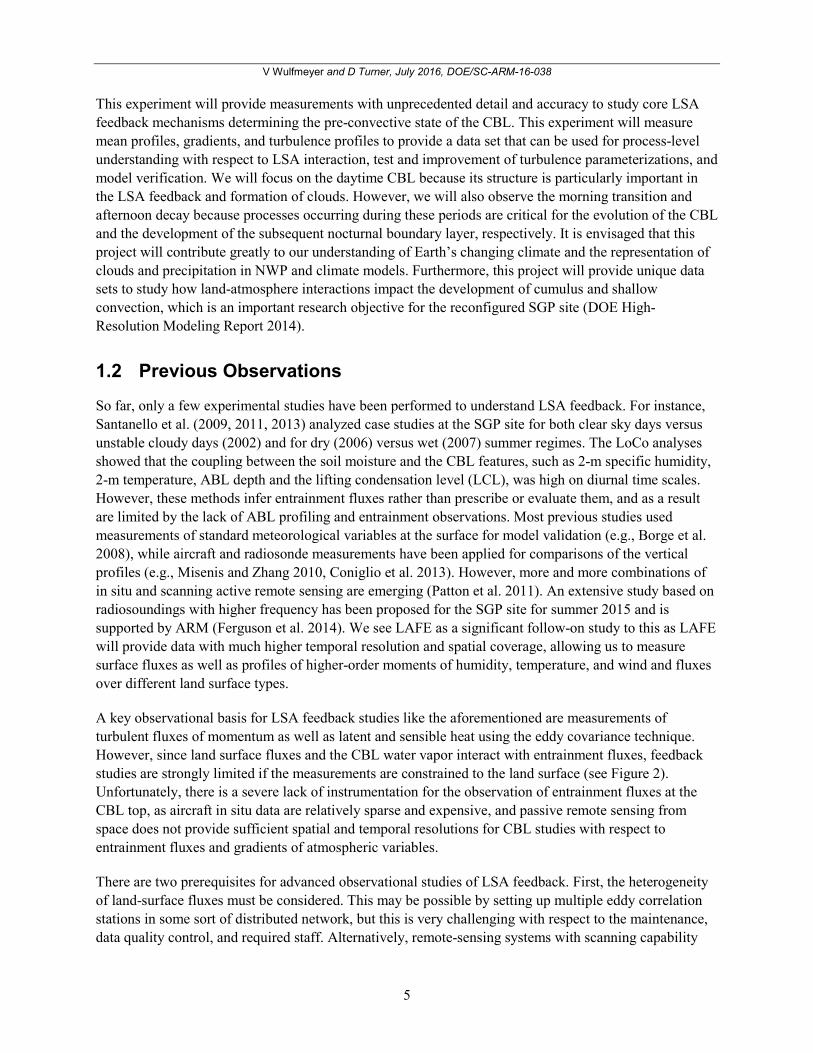
Figure 8. Measurement of a mixing-ratio variance profile (Wulfmeyer et al. 2010) demonstrating

turbulence resolution of the water vapor and temperature Raman lidar during daytime.

The water vapor and temperature Raman lidar was upgraded with new detection electronics in 2004, which greatly increased its signal-to-noise ratio (SNR) (Ferrare et al. 2006, Newsom et al. 2009) allowing 10-s profiles of aerosol backscatter and water-vapor mixing ratio to be observed. Channels sensitive to rotational Raman scattering by nitrogen and oxygen were added in 2005, allowing the system to also profile temperature (Newsom et al. 2013). Turbulence profiles from the 10-s water-vapor mixing ratio data from the high channels have been demonstrated for the first time by Wulfmeyer et al. (2010) and evaluated relative to turbulence observations made in situ by aircraft (Turner et al. 2014a). Data from 300 afternoon cases were analyzed to provide the first long-term climatology of water-vapor turbulence at a mid-latitude site (Turner et al. 2014b). An example of a water-vapor variance profile observed by the water vapor and temperature Raman lidar, together with its uncertainty, is provided in Figure 8 (Wulfmeyer et al. 2010; see also Turner et al. 2014a, b).

The SGP Doppler lidar is a Halo Photonics Streamline system (Pearson et al. 2009). This system uses a heterodyning approach to determine the Doppler velocity along the radial dimension. It uses a transceiver to transmit 1.5 µm pulses of light into the atmosphere at 20 kHz, and backscatter data are typically co-added to provide 1-s resolution. A two-axis scanner allows the system to measure radial velocities along any azimuth or elevation.

The ARM program typically operates its SGP Doppler lidar in two modes. The primary mode is vertically pointing, which provides 1-s measurements of vertical velocity. These observations have been used to derive the variance, the third-order moment, and the skewness of the vertical velocity field (e.g., Hogan et al. 2009, Klein et al. 2015). The ARM facility also has its SGP Doppler lidar perform constant elevation azimuth scans at regular intervals. From these scans, the horizontal wind as a function of range can be derived from the radial velocities measured along different azimuths using the velocity azimuth display (VAD) technique. The wind speed and direction derived from the Doppler lidar using this approach compares very well with other in situ and remote-sensing techniques (e.g., Klein et al. 2015).

The NDIAL instrument is described in detail in Spuler et al. (2015). In general, the eye-safe diode-laser-based DIAL is capable of continuous unattended operation in all conditions both day and night. The vertically pointing instrument is capable of accurately measuring water vapor, with a 150 m range


11

resolution and 10 min temporal resolution, from 300 m to 4 km above ground level (or cloud base, whichever comes first). Enhanced performance is expected during typical summertime conditions when the water vapor concentration is higher, such as 30-s temporal resolution in the lower 2 km. An example of the NDIAL data at 10-min, 75-m resolution is shown in Figure 9.

Figure 9. NDIAL and AERI data collected during FRAPPE from 22-25 July, 2014. The continuous

observations of water-vapor mixing ratio by the DIAL and AERI (both with 10-min resolution here) compare very well, especially the build-up and sharp decrease in moisture due to mesoscale circulations. The AERI-retrieved temperature shows marked variability.

The NDIAL will be deployed at the Garber X-band radar site (I5), which is approximately 15 km SSW of the SGP central facility. This site is chosen because the primary direction for boundary-layer winds is from the southwest in August. The placement of the NDIAL in this location will enable us to characterize the inhomogeneities in the water-vapor field along the wind direction. This deployment strategy allows us to look at inhomogeneities in the water-vapor field due to advection at three different scales: on the order of 100 km by the network of four AERIs/DLs at the boundary facilities (Figure 7), along this 15 km distance between the NDIAL and the water vapor and temperature Raman lidar, and along the 5 km RHI path observed by the scanning UDIAL. If another DL is available, we would request that it be deployed at the NDIAL site to determine horizontal wind profiles and to study whether the resolution of the NDIAL is high enough to resolve latent heat flux profiles.

1.3.2 Second LAFE Component

This component consists of the NOAA HRDL for wind, the UDIAL for water vapor, and the URL for temperature measurements. These systems will perform continuous RHIs scans along a single azimuth direction from the surface to the lower troposphere, including the interfacial layer at the CBL top. Furthermore, two EB stations will operated under this scan path.

The HRDL is built in a mobile seatainer (see Figure 10, left photo) (Grund et al. 2001). The transmitter is based on an eye-safe, frequency-stable laser (Wulfmeyer et al. 2000) operating with a repetition rate of 200 Hz and at the eye-safe wavelength of 2.02 µm. In combination with a 3D scanner, the SNR of LOS


12

wind measurements is high enough to perform rapid horizontal and RHI scans to study the horizontal and vertical structure of the wind field. VAD scans can also be used to create horizontal wind profiles from close to the surface to the top of the CBL. In vertically staring mode, HRDL can provide vertical velocity measurements from 200 m above the ground to top of the boundary layer with 30-m range resolution.

Figure 10. Left: The High-Resolution Doppler Lidar (HRDL) deployed in a ground-based configuration.

Right: Vertical velocity measurements made by HRDL during the LUMEX 2014 field experiment conducted in Erie, Colorado, showing the propagation of a large-scale convective event. The time is in UTC. The measurements are made at 2 Hz rate and 30-m spatial resolution.

The excellent resolution and range of HRDL is demonstrated in Figure 10, right panel. The laser pulse energy and the system efficiency are high enough to perform measurements throughout the entire CBL up to 3-4 km. In contrast, the signal strengths from commercially available DLs often degrade significantly before the top of the CBL (due to a reduced concentration of aerosol particles caused by entrainment of cleaner air from the free troposphere) and thus are unable to capture a part of the entrainment processes. The HRDL is very important part of LAFE because its high signal-to-noise ratio (SNR) and spatial resolution allow for covering the entire interfacial layer and the imbedded entrainment processes, in combination with a large range and temporal resolution of various scan patterns. This campaign would be the first time that HRDL would be collocated with the scanning UDIAL and URL systems to take advantage of their synergy.

The performance of the UHOH lidar systems in comparison to other remote-sensing systems is discussed in Wulfmeyer et al. (2015a). The UDIAL is a mobile, 3D scanning water vapor remote-sensing system (Späth et al. 2016). It is based on a high-power laser transmitter operating around 820 nm with a repetition rate of 200 Hz and an 80-cm scanner. As demonstrated in Wulfmeyer et al. (2015a, 2016) and Muppa et al. (2016), the UDIAL is a world-class, unique, ground-based, remote-sensing system for water-vapor profiling with the highest accuracy (error < 2 %) as well as temporal and spatial resolutions (10 s, 50 m typically). The mobile trailer is shown in Figure 11, left panel, and the large scanner is shown in the right panel.


13

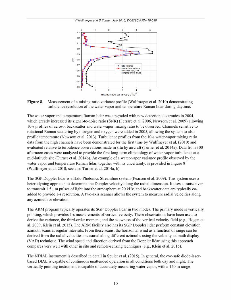
Figure 11. The UHOH 3D scanning WV DIAL. Left: Mobile trailer. Right: 80-cm 3D scanner.

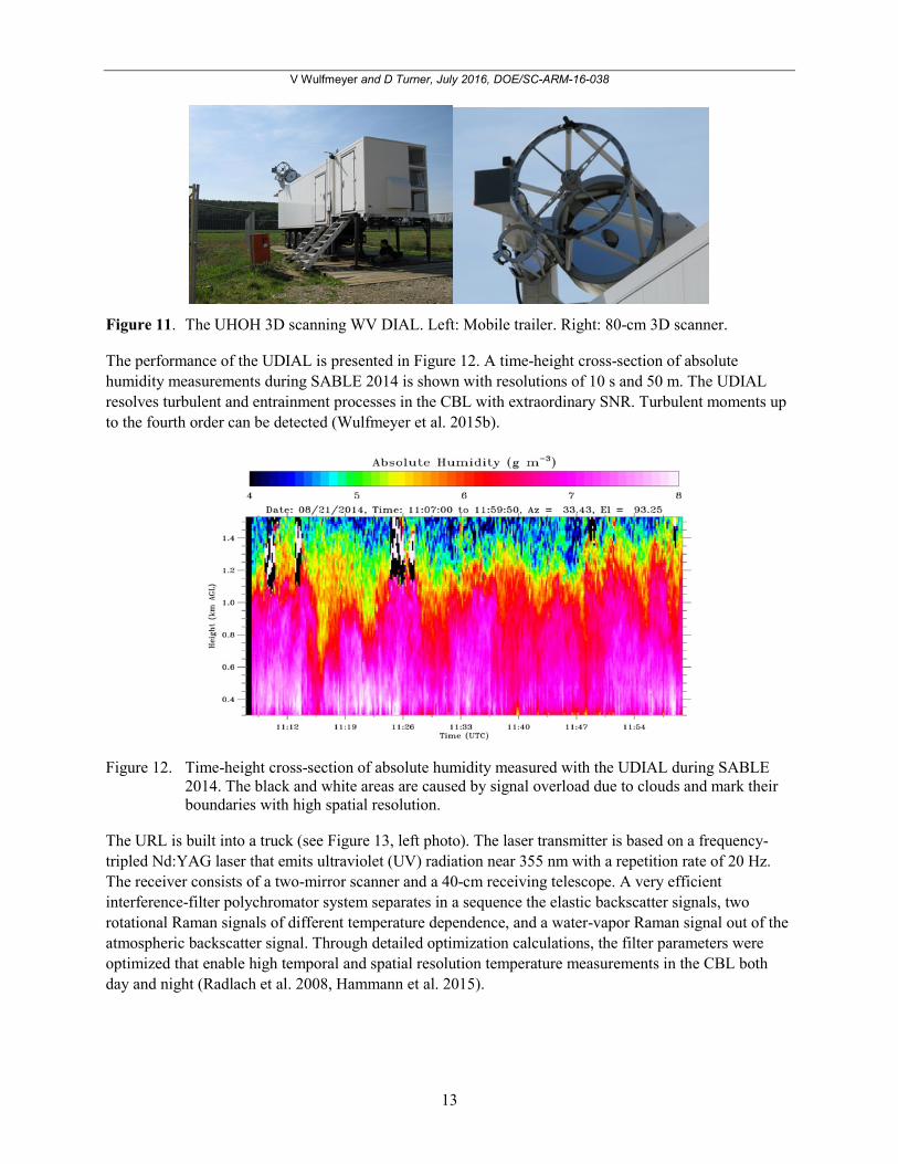
The performance of the UDIAL is presented in Figure 12. A time-height cross-section of absolute humidity measurements during SABLE 2014 is shown with resolutions of 10 s and 50 m. The UDIAL resolves turbulent and entrainment processes in the CBL with extraordinary SNR. Turbulent moments up to the fourth order can be detected (Wulfmeyer et al. 2015b).

Figure 12. Time-height cross-section of absolute humidity measured with the UDIAL during SABLE

2014. The black and white areas are caused by signal overload due to clouds and mark their boundaries with high spatial resolution.

The URL is built into a truck (see Figure 13, left photo). The laser transmitter is based on a frequency-tripled Nd:YAG laser that emits ultraviolet (UV) radiation near 355 nm with a repetition rate of 20 Hz. The receiver consists of a two-mirror scanner and a 40-cm receiving telescope. A very efficient interference-filter polychromator system separates in a sequence the elastic backscatter signals, two rotational Raman signals of different temperature dependence, and a water-vapor Raman signal out of the atmospheric backscatter signal. Through detailed optimization calculations, the filter parameters were optimized that enable high temporal and spatial resolution temperature measurements in the CBL both day and night (Radlach et al. 2008, Hammann et al. 2015).


14

Figure 13. The UHOH 3D-scanning temperature rotational Raman lidar (URL). Left: The truck. Right:

URL temperature profile measured with resolutions of 30 min and 100 m in comparison to an instantaneous radiosonde profile.

Figure 14. Turbulent fluctuations of temperature in the CBL measured with the URL between 11:04 and

12:00 UTC (around local noon) on 24 April, 2013, during the HOPE campaign. The white dotted line marks the mean CBL height zi of 1230 m above ground level.

Figure 13 (right panel) demonstrates that the resolution of the URL is high enough to determine the strength of the inversion at the CBL top (Hammann et al. 2015). This is an important scaling variable for studying turbulent exchange processes. Figure 14 confirms that turbulent fluctuations of temperature can be resolved during daytime. These measurements have been used for the profiling of temperature variance, which to our knowledge was the first time remote-sensing measurements of temperature variance profiling has been demonstrated (Behrendt et al. 2015).

The UHOH lidars are not eye-safe in the near range (within 175 m for the URL and 670 m for the UDIAL). However, during all measurement periods, we will ensure that all eye-safety regulations are met. This will be realized by operating a safety radar with the UDIAL, setting up a safety zone, and strongly cooperating with the Federal Aviation Administration (FAA) and Vance Air Force Base. In addition, a team member of UHOH will observe continuously the sector containing the lidar scan direction.


15

1.3.3 Third LAFE Component

The University of Wisconsin–Madison Space Science and Engineering Center (SSEC) Portable Atmospheric Research Center (SPARC) contains a suite of instruments to support the measurement of a wide range of earth system parameters. SPARC is a 36-foot trailer that is configured for field deployment and remote operation either by using internal generators or by connection to virtually any electrical power source found in the field. The current compliment of instruments in the SPARC includes an Atmospheric Emitted Radiance Interferometer (AERI), the High-Spectral-Resolution Lidar (HSRL), a ceilometer, a meteorology surface station, a radiosonde launch receiver, and a cross-track scanning Halo Streamline DL. Together, the AERI and HSRL instruments provide continuous temperature, water vapor, aerosol, and cloud extinction profiles.

The AERI is a fully automated, ground-based, passive infrared interferometer that measures downwelling atmospheric radiance from 3.3-18.2 µm (550 - 3000 cm-1) at 30-s temporal resolution with a spectral resolution of one wavenumber. Careful attention to calibration results gives an absolute calibration accuracy of better than 1% of the ambient radiance. The AERI instrument fore-optics consist of a scene mirror and two calibration blackbodies. These blackbodies are essential to provide a well-known, stable, hot and ambient temperature reference for calibration of the downwelling radiances. Temperature and humidity profiles are retrieved from the observed infrared radiance spectra (e.g., Turner and Löhnert 2014; see Figure 9 for an example). The AERI instrument can observe important mesoscale phenomena, such as boundary-layer evolution, cold/warm frontal passages, dry lines, and thunderstorm outflow boundaries. AERI temperature and moisture vertical retrievals provide data for stability index and planetary-boundary-layer monitoring.

The UW-SSEC lidar group has developed a series of HSRLs for both ground-based and aircraft platforms. The HSRL provides vertical profiles of optical depth, backscatter cross-section depolarization, and backscatter phase function. All HSRL measurements are absolutely calibrated by reference to molecular scattering that is measured at each point in the lidar profile. This enables the HSRL to measure backscatter cross-sections and optical depths without prior assumptions about the scattering properties of the atmosphere. Turbulent profiles have been derived from the HSRL-observed aerosol backscatter field, and the observed skewness profiles in CBLs were extremely similar to the water-vapor skewness profiles observed by the SRL (McNicholas and Turner 2014).

The Collaborative Lower Atmospheric Mobile Profiling System (CLAMPS) is a trailer-based remote-sensing facility that is very similar to SPARC. The CLAMPS is a joint University of Oklahoma (OU) and National Severe Storms Laboratory (NSSL) facility, and contains an AERI, a multichannel profiling microwave radiometer, and a Halo Streamline DL. Like the SPARC, it has its own generator to provide power, and can be remotely deployed.

We envision deploying the SPARC and CLAMPS on the side of fields that are close to the SGP site and approximately 1.5 and 3.0 km downrange of the central facility. These two mobile facilities would not be directly under the RHI path, but rather set to the side to allow the DLs in SPARC and CLAMPS to perform several RHI scans that intersect the RHI scan from the HRDL. The scans of the DLs at nearly right angles allows for profiles of u and v to be determined using dual-Doppler lidar techniques. The AERI observations from the two facilities will provide profiles of temperature and humidity (Turner and Löhnert 2014); the temperature profiles will be especially useful to look at small-scale differences near the surface that might be related to different land cover conditions.


16

1.3.4 Overall Sensor Synergy

Table 1 presents a summary of the variables using the sensor synergy proposed for LAFE. The key variables temperature T, mixing ratio m, absolute humidity ρ, and vertical wind w will be measured with a temporal resolution of 1-10 s and a range resolution of 30-60 m. The same resolution applies for the aerosol particle backscatter and extinction coefficients, and aerosol optical thickness (βPar, αPar, τPar) and the derived instantaneous CBL depth zi. Furthermore, the horizontal wind profile V and the cloud optical thickness τC are determined. From these results, the following variables will be derived: The TKE dissipation rate ε, profiles of the fluxes of water-vapor (latent heat) and the water-vapor variance <w’m’>, <w’ρ’>, <w’m’2>, <w’ρ’2>; the molecular destruction rates of humidity variances εm and ερ; profiles of the temperature flux (sensible heat) and the flux of temperature variance <w’T‘>, <w’T ‘2>; and the molecular destruction rate of temperature variance εT. The errors will be specified with respect to noise and sampling errors according to Lenschow et al. (2000), Wulfmeyer et al. (2010), Turner et al. (2014b), and Wulfmeyer et al. (2015c). The friction velocity u*; the surface latent and sensible heat fluxes Q0, S0; and the convective velocity, humidity, and temperature scales w*, q*, T* will be derived using MOST and compared with the surface fluxes measured with the EB stations.


17

Table 1. Variables measured by the instrument synergy during LAFE.

1 Also used to measure the instantaneous CBL depth zi using dT/dz, dm/dz, dρ/dz, and dβPar/dz 2 The measurement of molecular destruction rates of variances is explained in Wulfmeyer et al. (2015c) 3 In combination with u* measurements and MOST

Instrument Temperature1 Humidity1 Wind Fluxes Aerosols1 Clouds water vapor & temp. Raman lidar

T(z), dT/dz m(z), dm/dz, m’(z), <m’2>, <m‘3> βPar(z),αPar(z) Base, partly τC

UDIAL, vert. ρ(z),dρ/dz,ρ’(z),<ρ’2>,<ρ‘3>,<ρ‘4> βPar(z) Base, partly τC UDIAL, RHI 2D ρ, dρ/dz above canopy 2D βPar(z) field 2D cloud field

NDIAL ρ(z), dρ/dz βPar(z) Base

TRL, vert. T(z),dT/dz,T’(z), <T’2>,<T‘3>

βPar(z), αPar(z) Base, partly τC

TRL, RHI 2D T, dT/dz above canopy

2D βPar(z),αPar(z) field

2D cloud field

DL, vert. w(z), w’(z), <w’2>, <w‘3>, ε

βPar(z) Base, partly τC

DL, VAD scanning V(z), dV/dz HRDL, RHI 2D LOS wind field 2D βPar(z) field 2D cloud field

HSRL, vert. w(z), w’(z), <w’2>, <w‘3>, <w‘4>, ε

βPar(z), αPar(z),τPar(z) and turb. moments

Base, partly τC

Water vapor & temp. Raman lidar-DL, vert.

<w’m‘>,<w’m‘>/dz, <w’m‘2>, εm2

UDIAL-DL, vert. <w’ρ‘>, d<w’ρ ‘>/dz, <w’ρ ‘2>, ερ

TRL-DL, vert. <w’T‘>,d<w’T ‘>/dz, <w’T ‘2>, εT

Two DLs, cross-track scanning

u, v, and u* at crossing points

UDIAL-TRL, RHI Q0, S03 HRDL-UDIAL-TRL, RHI w*, q*, T*


18

2.0 Scientific Objectives and Research

2.1 Scientific Objectives

The overarching goal of LAFE is the study of LSA feedback in the SGP region during summertime covering different vegetation types, which would have different soil moisture conditions. This experiment has four scientific objectives:

I. Determine water vapor and vertical velocity turbulence and latent heat flux profiles, and investigate new similarity relationships for entrainment fluxes and variances.

II. Map surface momentum, sensible heat, and latent heat fluxes using a synergy of RHI scanning wind, humidity, and temperature lidar systems.

III. Characterize LSA feedback and the moisture budget at the SGP site by combining surface and CBL flux measurements as well as measurements of humidity advection in dependence of different soil moisture regimes.

IV. Verify LES runs and improve turbulence parameterizations in mesoscale models.

2.2 Strategies to Address the Objectives

2.2.1 Objective I

For addressing Objective I, we are taking advantage of LAFE component 1, the synergy between the high-resolution measurements of the SGP water vapor and temperature Raman lidar and the SGP DL. Using water-vapor and vertical velocity time series at different heights, their fluctuations can be measured with temporal resolutions of 1-10 s, typically. By means of the technique presented in Lenschow et al. (2000), these fluctuations are used to derive higher-order moments of mixing ratio and vertical velocity as well as their covariance, thus the latent heat flux. Wulfmeyer et al. (2010) demonstrated that mixing-ratio moments can be derived up to the third order from the water vapor and temperature Raman lidar with a temporal resolution of 30-60 min. Thus, daily cycles of turbulent properties can be measured. Turner et al. (2014b) showed that the high stability and the nearly continuous operation of the water vapor and temperature Raman lidar allowed for first studies of the statistics of turbulent properties in dependence of a variety of meteorological conditions.

So far, only the respective turbulent moments have been measured at the SGP site and have not been combined to derive the latent heat flux profiles4. Furthermore, the entrainment flux has not yet been related in detail to the properties of the interfacial layer, such as the strength of the inversion and the gradient Richardson number.

4 This was because the SGP water vapor and temperature Raman lidar and SGP Doppler lidar were separated by 300 m, thus prohibiting this analysis. This is being addressed by ARM moving these two instruments closer together in late 2015.


19

LAFE will explore this potential by its sensor synergy. Figures 17 and 18 demonstrate that indeed latent heat flux profiles can be derived with reasonable noise errors. The entrainment flux in this example was approximately 300 Wm-2, which is a reasonable value for the CBL. Considering the structure of the profile presented in Figure18, which represents to our knowledge the first attempt to profile the latent heat flux with the SGP water vapor and temperature Raman lidar, it seems also to be possible to estimate its divergence. This is a key ingredient for LSA feedback studies and the closure of the water budget (see also Objective III).

Figure 15. Left panel: Time-height cross-section of mixing ratio measurements and vertical wind

performed with the SGP water vapor and temperature Raman lidar and a collocated Halo DL from OU on November 9, 2012 (left and right, respectively) during the LABLE field experiment (Klein et al. 2015). The black bars are due to the switch to VAD scans for horizontal wind measurements. The lidar data can also be used to derive the ABL depth with very high accuracy using the water-vapor gradient.

Figure 16. The resulting latent heat flux profile derived with the data presented in Figure 17 using two

different vertical resolutions and including noise error bars.

Of course, considerably more data have to be collected for getting a deeper insight into the general capability of the SGP’s water vapor and temperature Raman lidar-Doppler lidar combination to measure latent heat-flux profiles with sufficiently low noise and sampling errors. The water vapor and temperature Raman lidar temperature data will also be evaluated to determine if accurate measurements of


20

temperature variance and skewness, as well as sensible heat flux, can be derived from these observations (Newson et al. 2013, Behrendt et al. 2015).

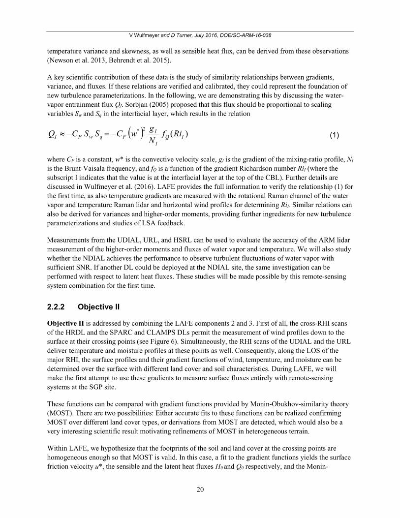
A key scientific contribution of these data is the study of similarity relationships between gradients, variance, and fluxes. If these relations are verified and calibrated, they could represent the foundation of new turbulence parameterizations. In the following, we are demonstrating this by discussing the water-vapor entrainment flux QI. Sorbjan (2005) proposed that this flux should be proportional to scaling variables Sw and Sq in the interfacial layer, which results in the relation

(1)

where CF is a constant, w* is the convective velocity scale, gI is the gradient of the mixing-ratio profile, NI is the Brunt-Vaisala frequency, and fQ is a function of the gradient Richardson number RiI (where the subscript I indicates that the value is at the interfacial layer at the top of the CBL). Further details are discussed in Wulfmeyer et al. (2016). LAFE provides the full information to verify the relationship (1) for the first time, as also temperature gradients are measured with the rotational Raman channel of the water vapor and temperature Raman lidar and horizontal wind profiles for determining RiI. Similar relations can also be derived for variances and higher-order moments, providing further ingredients for new turbulence parameterizations and studies of LSA feedback.

Measurements from the UDIAL, URL, and HSRL can be used to evaluate the accuracy of the ARM lidar measurement of the higher-order moments and fluxes of water vapor and temperature. We will also study whether the NDIAL achieves the performance to observe turbulent fluctuations of water vapor with sufficient SNR. If another DL could be deployed at the NDIAL site, the same investigation can be performed with respect to latent heat fluxes. These studies will be made possible by this remote-sensing system combination for the first time.

2.2.2 Objective II

Objective II is addressed by combining the LAFE components 2 and 3. First of all, the cross-RHI scans of the HRDL and the SPARC and CLAMPS DLs permit the measurement of wind profiles down to the surface at their crossing points (see Figure 6). Simultaneously, the RHI scans of the UDIAL and the URL deliver temperature and moisture profiles at these points as well. Consequently, along the LOS of the major RHI, the surface profiles and their gradient functions of wind, temperature, and moisture can be determined over the surface with different land cover and soil characteristics. During LAFE, we will make the first attempt to use these gradients to measure surface fluxes entirely with remote-sensing systems at the SGP site.

These functions can be compared with gradient functions provided by Monin-Obukhov-similarity theory (MOST). There are two possibilities: Either accurate fits to these functions can be realized confirming MOST over different land cover types, or derivations from MOST are detected, which would also be a very interesting scientific result motivating refinements of MOST in heterogeneous terrain.

Within LAFE, we hypothesize that the footprints of the soil and land cover at the crossing points are homogeneous enough so that MOST is valid. In this case, a fit to the gradient functions yields the surface friction velocity u*, the sensible and the latent heat fluxes H0 and Q0 respectively, and the Monin-

( ) )(2*IQ

I

IFqwFI Rif

NgwCSSCQ −=−≈


21

Obukhov length L. As several crossing points are realized, insight into the spatial variability of fluxes along the major RHI path is possible. The measurements of surface fluxes will be verified with the UHOH and OU EB stations and other eddy correlation (EC) stations at the SGP site further complemented with surface radiation as well as soil moisture and temperature measurements.

The question arises whether the range, noise level, and resolution of the UDIAL and URL scans are sufficient to resolve surface-layer gradients functions. Indeed, preliminary measurements performed during the HD(CP)2 in 2013 and the SABLE 2014 campaigns answer this question in a positive manner. For instance, Fig.19 presents two RHI scans during the HD(CP)2 campaign (Späth et al. 2016), revealing a strong heterogeneity of the water-vapor field confirming the high sensitivity and resolution of the UDIAL close to the surface.

Figure 17. 3D projection of slow scanning measurements of the UDIAL towards the LACROS and

JOYCE supersites during the HD(CP)2 campaign. These measurements were performed during IOP 5 on 20 April, 2013 be-tween 06:03 and 10:27 UTC. Each scan was performed within 10 min.

A zoom in the moisture scan close to the surface performed during SABLE 2014 is presented in Figure 20 (left panel). From these scans it is possible to derive near-surface water-vapor and temperature profiles. These are presented in Figure 20 (right panel), including the noise error bars. Thus, and to our knowledge for the first time, we were able to measure both the surface-layer water-vapor and temperature profiles using a combination of active remote-sensing systems. The SNR of the measurements is high enough to resolve the surface water-vapor and temperature profiles with errors <0.02 gm-3 and 0.02 K, respectively. A similar accuracy can be reached with respect to wind measurements using DLs. Therefore, these measurements confirm that we will be able to address Objective II.

During LAFE, we plan to operate the HRDL, the UDIAL, and the URL in RHI scanning mode for full daily cycles under various surface and mesoscale forcing conditions as well as different cloud coverage. As the gradients of wind, temperature, and moisture are measured simultaneously along the line of sight, over various land cover and soil moisture conditions, the daily cycle of fluxes will be derived and compared with EC measurements. We expect a temporal resolution of 30-60 min for these fluxes and a spatial resolution of a few 100 m. The availability of this array of state-of-the-art remote-sensing


22

instrumentation will be a unique opportunity to advance the understanding of boundary-layer processes in dependence on surface fluxes.

To maximize the potential scientific benefits of this month-long data set, we plan to expand the daily data-acquisition operations to include transition periods and to sample the nocturnal stable boundary layer (SBL) and associated low-level jet (LLJ). This will be achieved with little additional effort and will further extend our understanding of daytime CBL dynamics. Specifically, when not actively manned, NOAA’s HRDL system will be run autonomously, as will the CLAMPS, SPARC, and the NDIAL systems. These measurements will be complemented by the UDIAL and URL measurements, which are important for understanding the dynamics of the transitions and the nocturnal SBL, but require hands-on operation. These systems will be operated through the transition periods at several times through the project, and we also plan at least three 24-hr operations, all assuming the occurrence of appropriate atmospheric conditions.

Figure 18. Left panel: Surface-layer, high-resolution RHI scans of absolute humidity performed with the

UDIAL during SABLE 2014. Right panel: Combined active remote sensing of temperature and water-vapor profiles in the surface layer using a temporal average of 30 min (Wulfmeyer et al. 2015b, Späth et al. 2016).

Previous studies in the Great Plains regions of Kansas (October) and southeastern Colorado (September) using HRDL have yielded interesting relationships that can be tested with analysis procedures already developed (Banta et al. 2002, 2003, 2006; Banta 2008; Pichugina et al. 2008, 2010). As a bonus, these would be augmented with high-quality temperature and moisture profiles at high time resolution, with a consequent high probability of significantly advancing understanding of these poorly understood phenomena.

2.2.3 Objective III

The combination of variables measured during LAFE makes the estimation of the water-vapor budget possible. The water-vapor mixing ratio (m) budget equation is

(2) ''mwz

mVtm

∂∂

−=∇+∂∂


23

if other sources and sinks can be neglected. Higher-order budgets such as for mixing-ratio variance

(3)

may also be studied where mixed third-order turbulent moments occur. These will be measured with our LAFE synergy as well. Please note that both equations hold for a quasi-stationary CBL, which is assumed for all variables explained in Table 1. The first and the third terms of Equation 1 are measured using the water vapor and temperature Raman lidar-Doppler lidar combination. Further measurements of the first term are performed by the UDIAL, the NDIAL, and the AERI instruments, thereby improving the accuracy and consistency of the observations.

Crucial parts of Equations 2 and 3 are the advection terms, which are very difficult to measure. The LAFE design may enable us to estimate these with unprecedented accuracy. The 3D moisture gradient on different spatial scales will be determined using the AERI instrumentation in the environment of the central LAFE instrumentation, as well as the AERI and DLs that are part of the new boundary facility network installed as part of the SGP reconfiguration (Figures 6 and 7). The RHI scans of the UDIAL in combination with the NDIAL will enable us to measure the horizontal water-vapor gradient along the LOS of RHI that is oriented along the typical mean wind direction. Furthermore, the horizontal wind measurements of the Doppler lidar, the combination of the other DLs used during LAFE, and adding other wind-profile measurements at the SGP site such as radiosoundings and wind profilers will be used to get the best estimate of the horizontal wind profile.

Figure 19. Mixing diagrams for 8 September, 2009 between 7 and 17 UTC. Solid lines demonstrate the

simulated coevolution of Lq and Cpθ. Dashed colored lines are vectors that correspond to the land-surface fluxes (Vsfc), the advected fluxes (Vadv), and the entrainment fluxes (Ventr). The left panel (a) represent the simulations with WRF configured with NOAH LSM and the four PBL schemes (ACM2, MYJ, MYNN and YSU), while the right panel (b) shows the four WRF simulations configured with the combinations of the two PBL schemes (MYNN and YSU) and two LSMs (NOAH and NOAH-MP). Overlain are lines of constant θe (in K; black dashed) and RH (in %; orange dashed) (Milovac et al. 2016).

Observations of advection, the ABL budget, and entrainment processes are key to understanding the full nature of LSA coupling and assessing model physics (e.g., LSM and ABL schemes) in interactive mode.

mmwzz

mmwmVt

mε2''''2'

'22

2

−∂∂

−∂∂

−=∇+∂

∂


24

This has been demonstrated by research under the LoCo project, where the mixing diagram approaches of Betts (1992) and Santanello et al. (2009) are used to simultaneously quantify the behavior of surface fluxes (latent, sensible), ABL fluxes (entrainment, advection), and states (2-meter temperature, humidity). While LoCo has demonstrated model sensitivity to physics and parameters (e.g., Figure 21), these diagnostics have been limited in terms of model evaluation or development due to lack of ABL height, advection, and entrainment observations. The measurements proposed herein would thus have immediate impact on LoCo research by enabling not only couplings spread across models, but also accuracy and insight as to where development needs to be targeted.

2.2.4 Objective IV

Objective IV will evaluate turbulence parameterizations and perform model verification. An example for the parameterizations of entrainment fluxes and variances is presented in Equation 1 of Objective I. Validation and refinement of this equation may eventually lead to advanced representations of turbulent fluxes in mesoscale model turbulence parameterizations. Using WRF as an example, ensemble runs with different turbulence parameterizations such as those presented in Figure 21 can be performed over the SGP site. Their results can be compared with the LAFE measurements and investigated with respect to their accuracy. As operational LES runs for the SGP site are in preparation and these can be combined with mesoscale model runs with and without turbulence parameterizations, LAFE will be extremely timely for the analyses proposed within Objective IV.

The power of the LAFE measurements is illustrated here using the well-known YSU turbulence parameterization scheme. In this case, the water-vapor flux profile is parameterized as

(4)

where is the von-Karman constant, is a mixed-layer velocity scale (model output), and are

model constants, and is the Prandtl number at the top of the surface layer. The latter is interacting

with the surface-layer parameterizations via the stability functions for momentum and moisture .

The so-called counter-gradient term is parameterized according to

(5)

where is another model constant and is the vertical velocity at model level with . Further details are found in Milovac et al. (2016).

Of course, similar sets of equations can be derived for other local and non-local parameterizations as well as for parameterizations based on mass-flux schemes. LES model simulations will be performed, and computed higher-order, turbulent-moment profiles and flux pro-files will be compared against the lidar

( ) ( ) cz

zzzzzzwzK

zzKzK

zmzKzmw

m

v

i

i

is

mmm

+=

−−−+=

−=

=

+∂∂

−=

φφη

κ

γ

02

2

0

2

Pr,3exp1Pr1)Pr(,1)(

,)Pr()()(with)()(''

κ sw η c

0Pr

vφ mφ

mγ

ism zw

Qa0

0=γ

a 0sw izz 5.0=


25

observations from LAFE, as these profiles are not parameterized in LES models. These comparisons will be performed for routine LES runs for the SGP site, which are planned by ARM, but also for dedicated IOPs with the new WRF-NOAHMP-HYDRO model system that is operated at UHOH (Wulfmeyer et al. 2014, 2015b).

While LES simulations have traditionally been used for idealized and theoretical studies, these simulations will be driven by reanalysis and observational data, following Neggers et al. (2012). The obvious advantage is that these simulations can be expected to be very close to the observations, at least in a statistical sense. Relationships between surface fluxes, atmospheric turbulence, entrainment, and cloud formation to be found in the observations are likely to show up in these simulations as well, which would mean that the LES may serve as a virtual laboratory to test hypotheses. For instance, by breaking certain couplings in the LSA, one could figure out cause and effect for these feedbacks. LES could also assist in comparisons with validations of large-scale parameterizations, such as the YSU turbulence scheme described above; indeed, the original premise behind the testbed set-up (Neggers et al. 2012) was that parameterization schemes are usually designed against ideal and idealized data sets and may not hold as well against more realistic (continental) data. This is particularly true for parameterizations of the ABL and of ABL clouds.

There are many components where LES shares the weaknesses of mesoscale models. For instance, sub-filter-scale turbulence is still parameterized, which causes uncertainties around stable interfaces such as the surface layer and the entrainment interfacial layer—especially for coarser LES resolutions (100 m and coarser). The surface layer would be of particular interest here. This is not only because interactive soil models are relatively new in LES, and can therefore likely be optimized for the smaller scales, but also because typical MOST-based surface-layer parameterizations may not be valid in very high-resolution simulations. Data sets like the LAFE measurements will therefore be invaluable to improve the surface and soil parameterizations of LES and larger-scale models.

Obviously, due to the simultaneous measurement of fluxes and gradients of mean dynamics and thermodynamic variables, turbulence parameterizations and other performance measures of mesoscale model output can be studied in great detail.

3.0 Relevancy The ultimate goal of DOE’s Atmospheric System Research (ASR) program is to improve the understanding of a wide range of atmospheric processes and the representation of these processes in global climate models. Turbulent processes in the boundary layer occur on a range of scales, from millimeters to kilometers, and are responsible for the redistribution of heat, moisture, momentum, and aerosol throughout the boundary layer and into the free troposphere. In particular, the characterization of the moisture variance within the convective boundary layer is important for understanding the boundary-layer moisture budget, its impact on the formation of boundary-layer clouds, and its role as part of the trigger for deep convection in convective parameterizations. However, because turbulence works at scales much smaller than the resolution of most numerical models, turbulent mixing and transport must be parameterized.

The impact of the land surface on the atmosphere, and vice versa, is another high-priority research area for DOE. The properties of the land surface varies dramatically over short distances in most continental


26

locations, such as the SGP, and understanding how these relatively small scale inhomogeneities impact the atmospheric boundary layer and ultimately the cloudiness overhead is critical in order to represent these processes in climate models.

LAFE will provide a unique data set that will allow us to characterize the impact of land surface inhomogeneity on turbulent fluxes in the CBL and to quantify how this inhomogeneity affects the fluxes in the interfacial layer. Several of the investigators of this proposal are working on a set of new similarity relationships that were originally derived from LES simulations (Wulfmeyer et al. 2016) and need to be evaluated with data sets such as those to be collected during this experiment. These similarity relationships could form the basis of new parameterizations that link surface properties and large-scale environmental variables to turbulent characteristics of the convective boundary layer. Furthermore, this experiment will provide a data set that can be used to evaluate new parameterizations that have been suggested that connect large-scale geophysical variables that are predicted by cloud-resolving and global climate models with the turbulent profiles in the convective boundary layer.

The SGP site is being reconfigured by DOE to, in part, focus on land-atmosphere interactions and shallow convection and to support high-resolution numerical modeling of these processes. LAFE directly supports these research topics by attempting to characterize the small-scale inhomogeneities in water vapor (in particular) and temperature, quantifying profiles of variance and skewness in these fields, deriving fluxes of latent and sensible heat, and attempting to quantify the importance of advection on these profiles. By working across a range for scales (using the 5-km RHI, to the 15-km spacing between the NDIAL and the instruments at the central facility, to the 10-km diameter of the new SGP boundary facilities), LAFE investigators will look at the variability of water vapor and temperature at different scales and will evaluate their simulations to see if this variability is being simulated. This work will take advantage of the full range of capabilities at the newly reconfigured SGP site.

Dr. Wulfmeyer is a PI of the HD(CP)2 project in Germany (and Dr. Turner is collaborating closely with other HD(CP)2 PIs and is thus part of the community), which has the overarching goal to improve the representation of clouds and precipitation in climate models. This goal is strongly in line with the vision of LAFE, so that a realization of LAFE will foster international collaboration in the field of earth system process studies and simulations, particularly with respect to the representation of LSA interaction and feedback.

The proposed LAFE research addresses three of the five primary goals of DOE’s Climate and Environmental Sciences Division:1) the synthesis of new process knowledge and innovative computational methods to advance next-generation, integrated models of the human-earth system, 2) the development, testing, and simulation of process-level understanding of atmospheric systems and terrestrial ecosystems, extending from bedrock to the top of the vegetative canopy, and 3) enhancing the unique capabilities and impacts of the ARM Facility to advance the frontiers of climate and environmental science.

4.0 References Ansmann, A, J Fruntke, and R Engelmann. 2010. “Updraft and downdraft characterization with Doppler lidar: cloud-free versus cumuli-topped mixed layer.” Atmospheric Chemistry and Physics 10: 7845-7858.


27

Banta, RM. 2008. “Stable boundary layer regimes from the perspective of the low-level jet.” Special Issue, Acta Geophysica 56: 58-87.

Banta, RM, RK Newsom, JK Lundquist, YL Pichugina, RL Coulter, and L Mahrt. 2002. “Nocturnal low-level jet characteristics over Kansas during CASES-99.” Boundary-Layer Meteorology 105: 221-252.

Banta, RM, YL Pichugina, and RK Newsom. 2003. “Relationship between low-level jet properties and turbulence kinetic energy in the nocturnal stable boundary layer.” Journal of the Atmospheric Sciences 60: 2549-2555.

Banta, RM, YL Pichugina, and WA Brewer. 2006. “Turbulent velocity-variance profiles in the stable boundary layer generated by a nocturnal low-level jet.” Journal of the Atmospheric Sciences 63: 2700-2719.

Behrendt, A, V Wulfmeyer, A Riede, G Wagner, S Pal, H Bauer, M Radlach, and F Späth. 2009. “3-Dimensional observations of atmospheric humidity with a scanning differential absorption lidar.” In Richard H. Picard, Klaus Schäfer, Adolfo Comeron et al. (Eds.), Remote Sensing of Clouds and the Atmosphere XIV, SPIE Conference Proceeding Vol. 7475, ISBN: 9780819477804, 2009, Art. No. 74750L, DOI:10.1117/12.835143.

Behrendt, A, S Pal, F Aoshima, M Bender, A Blyth, U Corsmeier, J Cuesta, G Dick, M Dorninger, C Flamant, P Di Girolamo, T Gorgas, Y Huang, N Kalthoff, S Khodayar, H Mannstein, K Träumner, A Wieser, and V Wulfmeyer. 2011. “Observation of convection initiation processes with a suite of state-of-the-art research instruments during COPS IOP8b.” Quarterly Journal of the Royal Meteorological Society 137: 81–100, DOI:10.1002/qj.758.

Behrendt, A, V Wulfmeyer, E Hammann, SK Muppa, and S Pal. 2015. “Profiles of second- to forth-order moments of turbulent temperature fluctuations in the convective boundary layer: First measurements with rotational Raman lidar.” Atmospheric Chemistry and Physics 15: 5485-5500, DOI:10.5194/acp-15-5485-2015.

Betts, AK. 1992. “FIFE atmospheric boundary-layer budget methods.” Journal of Geophysical Research 97: D17, 18523–18531.

Borge, R, V Alexandrov, JJ del Vas, J Lumbreras, and E Rodríguez. 2008. “A comprehensive sensitivity analysis of the WRF model for air quality applications over the Iberian Peninsula.” Atmospheric Environment 42: 8560-8574.

Coniglio, MC, J Correia, PT Marsh, and F Kong. 2013. “Verification of convection-allowing WRF model forecasts of the planetary boundary layer using sounding observations.” Weather Forecasting 28: 842–862.

Cooper, DI, WE Eichinger, J Achuleta, L Hipps, CMU Neale, and JH Prueger. 2007. “An advanced method for deriving latent energy flux from a Scanning Raman Lidar.” Agronomy Journal 99: 272–284.

Corsmeier, U, N Kalthoff, C Barthlott, A Behrendt, P Di Girolamo, M Dorninger, F Aoshima, J Handwerker, C Kottmeier, H Mahlke, S Mobbs, G Vaughan, J Wickert, and V Wulfmeyer. 2011. “Driving processes for deep convection over complex terrain: A multiscale analysis of observations from


28

COPS-IOP 9c.” Quarterly Journal of the Royal Meteorological Society 137: 137–155, DOI:10.1002/qj.754.

Crook, NA. 1996. “Sensitivity of moist convection forced by boundary layer processes to low-level thermodynamic fields.” Monthly Weather Review 124: 1767-1785.

Cuijpers, JWM, and AAM Holtslag. 1998. “Impact of skewness and nonlocal effects on scalar and buoyancy fluxes in convective boundary layers.” Journal of the Atmospheric Sciences 55: 151–162.

Dirmeyer, PA, BA Cash, JL Kinter, C Stan, T Jung, L Marx, P Towers, N Wedi, JM Adams, EL Altshuler, B Huang, EK Jin, and J Manganello. 2012. “Evidence for enhanced land–atmosphere feedback in a warming climate.” Journal of Hydrometeorology 13: 981–995.

Dirmeyer, PA. 2014. “The cusp of major progress in predicting land-atmosphere interactions.” GEWEX News 24(1-2): 15-18.

DOE. 2014. Atmospheric Research measurement Climate Research Facility – Atmospheric System Research High-Resolution Modeling Workshop. DOE Climate and Environmental Sciences Division, DOE/SC-0169.

Ek, MB, and AAM Holtslag. 2004. “Influence of soil moisture on boundary layer cloud development.” Journal of Hydrometeorology 5: 86–99.

Ferguson, CR, JR Santanello, and P Gentine. 2014. Enhanced soundings for local coupling studies: 2015 ARM Climate Research Facility Field Campaign Science Plan. DOE/SC-ARM-16-023, www.arm.gov/publications/programdocs/doe-sc-arm-15-035.pdf

Ferrare, RA, DD Turner, M Clayton, B Schmid, J Redemann, D Covert, R Elleman, J Ogren, E Andrews, JEM Goldsmith, and H Johsson. 2006. “Evaluation of daytime measurements of aerosols and water vapor made by an operational Raman lidar over the Southern Great Plains.” Journal of Geophysical Research 111: D05S08, DOI:10.1029/2005JD005836.

Gentine, P, AAM Holtslag, F D’Andrea, and M Ek. 2013. “Surface and atmospheric controls on the onset of moist convection over land.” Journal of Hydrometeorology 14: 1443–1462.

Goldsmith, JEM, FH Blair, SE Bisson, and DD Turner. 1998. “Turn-key Raman lidar for profiling atmospheric water vapor, clouds, and aerosols.” Applied Optics 37: 4979-4990, DOI:10.1364/AO.37.004979.

Grisogono, B. 2010. “Generalizing “z-less” mixing length for stable boundary layers.” Quarterly Journal of the Royal Meteorological Society 136: 213–221.

Grund, CJ, RM Banta, JL George, JN Howell, MJ Post, RA Richter, and AM Weickmann. 2001. “High-resolution Doppler lidar for boundary layer and cloud research.” Journal of Atmospheric and Oceanic Technology 18: 376–393, DOI:10.1175/1520-0426(2001)018<0376:HRDLFB>2.0.CO;2.


29

Hammann, E, A Behrendt, F Le Mounier, and V Wulfmeyer. 2015. “Temperature profiling of the atmospheric boundary layer with rotational Raman lidar during the HD(CP)2 Observational Prototype Experiment.” Atmospheric Chemistry and Physics 15: 2867-2881, DOI:10.5194/acp-15-2867-2015.

Hogan, RJ, ALM Grant, AJ Illingworth, GN Pearson, and EJ O’Connor. 2009. “Vertical velocity variance and skewness in clear and cloud-topped boundary layers as revealed by Doppler lidar.” Quarterly Journal of the Royal Meteorological Society 135: 635-643, DOI:10.1002/qj.413.

Holtslag, AAM, and B Boville. 1993. “Local versus nonlocal boundary-layer diffusion in a global climate model.” Journal of Climate 6(10): 1825-1842.

Hong, SY. 2010. “A new stable boundary-layer mixing scheme and its impact on the simulated East Asian summer monsoon.” Quarterly Journal of the Royal Meteorological Society 136: 1481–1496.

Hong, S-Y, Y Noh, and J Dudhia. 2006. “A new vertical diffusion package with an explicit treatment of entrainment processes.” Monthly Weather Review 134: 2318-2341.

Huang, J, X Lee, and EG Patton. 2011. “Entrainment and budgets of heat, water vapor, and carbon dioxide in a convective boundary layer driven by time-varying forcing.” Journal of Geophysical Research 116: D06308.

Jaeger, EB, and S Seneviratne. 2011. “Impact of soil moisture-atmosphere coupling on European climate extremes and trends in a regional climate model.” Climate Dynamics 36: 1919–1939.

Klein, P, TA Bonin, JF Newman, DD Turner, PB Chilson, CE Wainwright, WG Blumberg, S Mishra, M. Carney, EP Jacobsen, and RK Newsom. 2015. “LABLE: A multi-institutional, student-led, atmospheric boundary layer experiment.” Bulletin of the American Meteorological Society, accepted.

Kotlarski, S, K Keuler, M Déqué, A Gobiet, K Görgen, D Jacob, D Lüthi, E van Meijgard, G Nikulin, M Suklitsch, C Teichmann, RVautard, K Warrach-Sagi, and V Wulfmeyer. 2014. “Regional climate modeling on European scales: A joint standard evaluation of the Euro-CORDEX RCM ensemble.” Geoscientific Model Development 7: 1297–1333, DOI:10.5194/gmd-7-1297-2014.

Lenderink, G, and E van Meijgaard. 2008. “Increase in hourly precipitation extremes be-yond expectations from temperature changes.” Nature Geoscience 1: 511–514.

Lenschow, DH, J Mann, and L Kristensen. 1994. “How long is long enough when measuring fluxes and other turbulence statistics?” Journal of Atmospheric and Oceanic Technology 11: 661–673.

Lenschow, DH, V Wulfmeyer, and C Senff. 2000. “Measuring second-through-fourth-order moments in noisy data.” Journal of Atmospheric and Oceanic Technology 17: 1330-1347, DOI:10.1175/1520-0426(2000)017<1330:MSTFOM>2.0.CO;2.

Lenschow, DH, M Lothon, SD Mayor, PP Sullivan, and G Canut. 2012. “A comparison of higher-order vertical velocity moments in the convective boundary layer from lidar with in situ measurements and large-eddy simulation.” Boundary-Layer Meteorology 143: 107-123.


30

Mahmood, R, RA Pielke, KG Hubbard, D Niyogi, PA Dirmeyer, C McAlpine, AM Carleton, R Hale, S Gameda, A Beltrán-Przekurat, B Baker, R McNider, DR Legates, M Shepherd, J Du, PD Blanken, OW Frauenfeld, US Nair, and S Fall. 2013. “Land cover changes and their biogeophysical effects on climate.” International Journal of Climatology 34: 929–953.

McNicholas, C, and DD Turner. 2014: “Characterizing the convective boundary layer turbulence with a high spectral resolution lidar.” Journal of Geophysical Research 119: 12910-12927, DOI:10.1002/2014JD021867

Mellor, GL, and T Yamada. 1974. “A hierarchy of turbulence closure models for planetary boundary layers.” Journal of the Atmospheric Sciences 31: 1791-1806.

Mellor, GL, and T Yamada. 1982. “Development of a turbulence closure model for geo-physical fluid problems.” Review of Geophysics and Space Physics 20: 851-875.

Milovac, J, K Warrach Sagi, J Ingwersen, A Behrendt, F Späth, H-D Wizemann, and V Wulfmeyer. 2014. Sensitivity of the WRF model to boundary-layer and land-surface parameterizations: comparisons with differential absorption lidar and eddy covariance measurements. 7th International Scientific Conference on the Global Water and Energy Cycle, Den Haag, The Netherlands, July 14-17, 2014.

Milovac, J, K Warrach-Sagi, A Behrendt, F Späth, J Ingwersen, and V Wulfmeyer. 2015. “Investigation of PBL schemes combining the WRF model simulations with scanning water vapor differential absorption lidar measurements.” Journal of Geophysical Research, DOI:10.1002/2015JD023927, in press.

Misenis, C, and Y Zhang. 2010. “An examination of sensitivity of WRF/Chem predictions to physical parameterizations, horizontal grid spacing, and nesting options.” Atmospheric Research 97: 315–334.

Muppa, SK, A Behrendt, F Späth, V Wulfmeyer, S Metzendorf, and A Riede. 2016. “Turbulent humidity fluctuations in the convective boundary layer: Case studies using water vapour differential absorption lidar measurements.” Boundary-Layer Meteorology 158: 43-66, DOI:10.1007/s10546-015-0078-9.

Neggers, RAJ, AP Siebesma, and T Heus. 2012. “Continuous single-column model evaluation at a permanent meteorological supersite”. Bulletin of the American Meteorological Society 93: 1389–1400.

Newsom, RK, DD Turner, B Mielke, M Clayton, R Ferrare, and C Sivaraman. 2009. “The use of simultaneous analog and photon counting detection for Raman lidar.” Applied Optics 48: 3903-3914, DOI:10.1364/AO.48.003903.

Newsom, RK, DD Turner, and JEM Goldsmith. 2013. “Long-term evaluation of temperature profiles measured by an operational Raman lidar.” Journal of Atmospheric and Oceanic Technology 30: 1616-1634, DOI:10.1175/JTECH-D-12-00138.1.

Noh, Y, WG Cheon, SY Hong, and S Raasch. 2010. “Improvement of the K-profile model for the planetary boundary layer based on large eddy simulation data.” Boundary-Layer Meteorology 107: 401–427.


31

Pal, S, A Behrendt, and V Wulfmeyer. 2010. “Elastic-backscatter lidar based characterization of the convective boundary layer and investigation of related statistics.” Annals of Geophysics 28: 825-847, DOI:10.5194/angeo-28-825-2010.

Patton, EG, TW Horst, PP Sullivan, DH Lenschow, SP Oncley, WOJ Brown, SP Burns, AB Guenther, A Held, T Karl, SD Mayor, LV Rizzo, SM Spuler, J Sun, AA Turnipseed, EJ Allwine, SL Edburg, BK Lamb, R Avissar, RJ Calhoun, J Kleissl, WJ Massman, KT Paw U, and JC Weil. 2011. “The canopy horizontal array turbulence study.” Bulletin of the American Meteorological Society 92: 593-611, DOI:10.1175/2010BAMS2614.1.

Pearson, GH, F Davies, and CG Collier. 2009. “An analysis of the performance of the UFAM pulsed Doppler lidar for observing the boundary layer.” Journal of Atmospheric and Oceanic Technology 26, 240-250.

Pichugina, YL, RM Banta, B Jonkman, ND Kelley, RK Newsom, SC Tucker, and WA Brewer. 2008. “Horizontal-velocity and variance measurements in the stable boundary layer using Doppler-lidar: Sensitivity to averaging procedures.” Journal of Atmospheric and Oceanic Technology 24: 1307–1327.

Pichugina, YL, and RM Banta. 2010. “Stable boundary-layer depth from high-resolution measurements of the mean wind profile.” Journal of Applied Meteorology and Climatology 49: 20-35.

Prandtl, L, 1942. Führer durch die Strömungslehre. Vieweg und Sohn, Braunschweig, 648 pp.

Radlach, M, A Behrendt, and V Wulfmeyer. 2008. “Scanning rotational Raman lidar at 355 nm for the measurement of tropospheric temperature fields.” Atmospheric Chemistry and Physics 8: 159-169, DOI:10.5194/acp-8-159-2008.

Rasmussen, SH, MB Butts, SM Lerer, and JC Refsgaard. 2012: “Parameterization and scaling of the land surface model for use in a coupled climate-hydrological model.” Journal of Hydrology 426: 63–78.

Santanello, JA, CD Peters-Lidard, SV Kumar, C Alonge, and W-K Tao. 2009. “A modeling and observational framework for diagnosing local land–atmosphere coupling on diurnal time scales.” Journal of Hydrometeorology 10: 577–599.

Santanello, JA, CD Peters-Lidard, and SV Kumar. 2011. “Diagnosing the sensitivity of local land–atmosphere coupling via the soil moisture–boundary layer interaction.” Journal of Hydrometeorology 12: 766–786.

Santanello, JA, CD Peters-Lidard, A Kennedy, and SV Kumar. 2013. “Diagnosing the nature of land–atmosphere coupling: A case study of dry/wet extremes in the U.S. Southern Great Plains.” Journal of Hydrometeorology 14: 3–24.

Seneviratne, SI, T Corti, EL Davin, M Hirschi, EB Jaeger, I Lehner, B Orlowski, and AJ Teuling. 2010. “Investigating soil moisture-climate interactions in a changing climate: a review.” Earth-Science Review 99: 125-161.

Senff, C, J Bösenberg, and G Peters, 1994. “Measurement of water vapor flux profiles in the convective boundary layer with lidar and radar RASS.” Journal Atmospheric Oceanic Technology 11: 85.


32

Sherwood, SC, R Roca, TM Weckwerth, and NG Andronova, 2010: “Tropospheric water vapor, convection, and climate.” Review of Geophysics 48: RG2001, DOI:10.1029/2009RG000301.

Sorbjan, Z. 2005. “Statistics of scalar fields in the atmospheric boundary layer based on large-eddy simulations. Part I: Free convection.” Boundary-Layer Meteorology 116: 467-486.

Späth, F, A Behrendt, SK Muppa, S Metzendorf, A Riede, and V Wulfmeyer. 2016. “3D water vapor fields in the atmospheric boundary layer observed with scanning differential absorption lidar.” Atmospheric Measurement Techniques 9: 1701-1720, DOI:10.5194/amt-2015-393.

Spuler, SM, KS Repasky, D Moen, B Morley, M Hayman, and AR Nehrir. 2015. “Field-deployable diode-laser-based DIAL for profiling water vapor.” Atmospheric Measurement Techniques 8: 1073-1087.

Stéfanon, M, P Drobinski, F D’Andrea, C Lebeaupin-Brossier, and S Bastin. 2014. “Soil moisture-temperature feedbacks at meso-scale during summer heat waves over Western Europe.” Climate Dynamics 42: 1309–1324.

Stull, RB. 1988. An Introduction to Boundary Layer Meteorology. Kluwer Academic Publishers, Dordrecht, 666 pp.

Taylor, CM, RAM de Jeu, F Guichard, PP Harris, and WA Dorigo. 2012. “Afternoon rain more likely over drier soils.” Nature 489: 423–426.

Teixeira, J, and S Cheinet. 2004. “A simple mixing length formulation for the eddy-diffusivity parameterization of dry convection. “Boundary-Layer Meteorology 110: 435–453.

Troen, IB, and L Mahrt. 1986. “A simple model of the atmospheric boundary layer; sensitivity to surface evaporation.” Boundary-Layer Meteorology 37: 129–148.

Tucker, SC, WA Brewer, RM Banta, C Senff, SP Sandberg, DC Law, AM Weickmann, and RM Hardesty. 2009. “Doppler lidar estimation of mixing height using turbulence, shear, and aerosol profiles.” Journal of Atmospheric and Oceanic Technology 26: 673–688, DOI:10.1175/2008JTECHA1157.1.

Turner, DD, and JEM Goldsmith. 1999. “Twenty-four-hour Raman lidar water vapor measurements during the Atmospheric Radiation Measurement Program's 1996 and 1997 water vapor intensive observation periods.” Journal of Atmospheric and Oceanic Technology 16: 1062-1076.

Turner, DD, RA Ferrare, LA Heilman Brasseur, WF Feltz, and TP Tooman. 2002: “Automated retrievals of water vapor and aerosol profiles from an operational Raman lidar.” Journal of Atmospheric and Oceanic Technology 19: 37-50, DOI:10.1175/1520-0426(2002)019<0037:AROWVA>2.0.CO;2.

Turner, DD, RA Ferrare, V Wulfmeyer, and AJ Scarino. 2014a. “Aircraft evaluation of ground-based Raman lidar water vapor turbulence profiles in convective mixed layers.” Journal of Atmospheric and Oceanic Technology 31: 1078-1088, DOI:10.1175/JTECH-D-13-00075-1.

Turner, DD, V Wulfmeyer, LK Berg, and JH Schween. 2014b. “Water vapor turbulence profiles in stationary continental convective mixed layers.” Journal of Geophysical Research 119: 11151-11165, DOI:10.1002/2014JD022202.


33

Turner, DD, and U Löhnert. 2014. “Information content and uncertainties in thermodynamic profiles and liquid cloud properties retrieved from the ground-based Atmospheric Emitted Radiance Interferometer (AERI).” Journal of Applied Meteorology and Climatology 53, 752-771, DOI:10.1175/JAMC-D-13-0126.1.

Van den Hurk, B, M Best, P Dirmeyer, A Pitman, J Polcher, and J Santanello. 2011. “Acceleration of land surface model development over a decade of Glass.” Bulletin of the American Meteorological Society 92: 1593–1600.

Vautard, R, A Gobiet, D Jacob, M Belda, A Colette, M Déqué, J Fernández, M García-Díez, K Goergen, I Güttler, T Halenka, T Karacostas, E Katragkou, K Keuler, S Ko-tlarski, S Mayer, E van Meijgaard, G Nikulin, M Patarčić, J Scinocca, S Sobolowski, M Suklitsch, C Teichmann, K Warrach-Sagi, V Wulfmeyer, and P Yiou. 2013. “The simulation of European heat waves from an ensemble of regional climate models within the EURO-CORDEX project.” Climate Dynamics 41: 2555-2575, DOI:10.1007/s00382-013-1714-z.

Wagner, G, V Wulfmeyer, F Späth, A Behrendt, and M Schiller. 2013. “Performance and specifications of a pulsed high-power single-frequency Ti:Sapphire laser for water-vapor differential absorption lidar.” Applied Optics 52: 2454-2469, DOI:10.1364/AO.52.002454.

Warrach-Sagi, K, T Schwitalla, V Wulfmeyer, and H-S Bauer. 2013. “Evaluation of a cli-mate simulation based on the WRF-NOAH model system: Precipitation in Germany.” Climate Dynamics 41: 755-774, DOI:10.1007/s00382-013-1727-7.

Weng, W, and P Taylor. 2003. “On modelling the one-dimensional atmospheric boundary layer.” Boundary-Layer Meteorology 107: 371–400.

Wulfmeyer, V, 1999a. “Investigation of turbulent processes in the lower troposphere with water-vapor DIAL and Radar-RASS.” Journal of the Atmospheric Sciences 56: 1055-1076, DOI:10.1175/1520-0469(1999)056<1055:IOTPIT>2.0.CO;2.

Wulfmeyer, V. 1999b. “Investigations of humidity skewness and variance profiles in the convective boundary layer and comparison of the latter with large eddy simulation results.” Journal of the Atmospheric Sciences 56: 1077-1087, DOI:10.1175/1520-0469(1999)056<1077:IOHSAV>2.0.CO;2.

Wulfmeyer, V, M Randall, A Brewer, and RM Hardesty. 2000. “2-µm Doppler lidar transmitter with high frequency stability and low chirp.” Optical Letters 25: 1228-1230, DOI:10.1364/OL.25.001228.

Wulfmeyer, V, and T Janjić. 2005. “Twenty-four-hour observations of the marine boundary layer using shipborne NOAA high-resolution Doppler lidar.” Journal of Applied Meteorology 44: 1723-1744, DOI:10.1175/JAM2296.1.

Wulfmeyer, V, DD Turner, S Pal, and E Wagner. 2010. “Can water vapour Raman lidar resolve profiles of turbulent variables in the convective boundary layer?” Boundary-Layer Meteorology 136: 253-284, DOI:10.1007/s10546-010-9494-z.


34

Wulfmeyer, V, and 54 coauthors. 2011. “The Convective and Orographically Induced Precipitation Study (COPS): The scientific strategy, the field phase, and first highlights.” Quarterly Journal of the Royal Meteorological Society 137: 3-30, DOI:10.1002/qj.752.

Wulfmeyer, V, et al., 2014. Consistent hydro-meteorological large eddy simulation of water budgets in mesoscale catchments: Overkill or necessity? AGU Chapman Conference, Luxembourg City, Luxembourg, September 23-26, 2014.

Wulfmeyer, V, RM Hardesty, DD Turner, A Behrendt, M Cadeddu, P Di Girolamo, P Schlüssel, J van Baelen, and F Zus. 2015a. “A review of the remote sensing of lower-tropospheric thermodynamic profiles and its indispensable role for the understanding and the simulation of water and energy cycles.” Review of Geophysics 53: 819-895, DOI:10.1002/2014RG000476.

Wulfmeyer, V., and the SABLE Team. 2015b. New Concepts for Studying Land-Surface-Atmosphere Feedback Based on a new Lidar Synergy and Grey Zone Simulations. EGU General Assembly, EGU2015-5054, Vienna, Austria, April 12-17, 2015.

Wulfmeyer, V, A Behrendt, Z Sorbjan, DD Turner, and RM Hardesty. 2016. “Determination of convective boundary layer entrainment fluxes, dissipation rates, and the molecular destruction of variances: Theoretical description and a strategy for its confirmation with a novel lidar system synergy.” Journal of the Atmospheric Sciences 73: 667-692, DOI:10.1175/JAS-D-14-0392.1.

Zolina, O, C Simmer, K Belyaev, SK Gulev, and P Koltermann. 2013. “Changes in the duration of European wet and dry spells during the last 60 years.” Journal of Climate 26: 2022–2047.

land-atmosphere feedback experiment (lafe) … feedback experiment (lafe) science plan . ... the...

Documents