Lake Photosynthesis

1 Introduction

Remember our problem: How much photosynthesis occurs in a lake?

In this lab, we will apply what we have learned about the relationship between photosynthesis andlight intensity to the problem of estimating the total amount of photosynthesis in a lake. To solvethis problem, it will be your task to synthesize Beer’s Law, the effect of light on photosynthesis,and the geometry of the lake. We will accomplish this by means of a mathematical model of theexperiment. As we will see, one of the main uses of mathematical models is to scale-up from thesmall scale of a laboratory experiment to the large scale of a whole lake. This activity is notwithout problems, but the model makes explicit all of our assumptions so that we can improve ourcalculations and observations.

For your homework, you will use your laboratory experiments to calculate the total amount ofphotosynthesis in two very different lakes: Bear Lake, Utah on the Idaho-Utah border and theGreat Salt Lake, Utah, near Salt Lake City, Utah. As the two photographs indicate the two lakesare very different geologically and morphologically. Bear Lake is deep and clear; the Great SaltLake is shallow and turbid.

2 Guessing the Effect of Light

How does light affect the rate of photosynthesis? We all know light is required for photosyn-thesis, but what is the precise quantitative relation between the amount of light and the rate ofphotoysnthesis?

2.1 Your Job

Use graph paper and draw some plausible curves for the effect of light on photosynthesis rate.While you are doing this, answer the following questions.

1. What is the independent variable in the question? What is the causal agent in thequestion?

2. What is the dependent variable in the question? What is the effect in the question?

3. What are the units and range of light intensity? (Think back to the previous lab.) Changethe plot x-axis to be the name of the independent variable with units in parentheses. Forexamples, “Chocolate Milk (liters).”

4. What are the units and range of photosynthesis? (You have several choices for units dependingon the experimental set-up. Check you lab manual.) Change the plot y-axis to the dependentvariable with units in parentheses. For example, “Speed of Flying Toasters (flaps/sec).”

5. For the possible curves of photosynthesis rate:

(a) If there is no light, what will be the rate?

(b) If the light is very, very, very high, what will happen to the rate? [Hint: Photoinhibition]

–1–

(c) If the light is 0.0 and then increases gradually to an intermediate level, how will the rateincrease? You have basically 4 choices. Will the rate increase slowly at first, then slowdown? Will it increase slowly, but never slow down? Will it increase rapidly, then slowdown? Or, will it increase rapidly and never slow down?

6. Draw the possibilities that you think are plausible.

Wait for the instructor to re-convene the class and discuss your predictions.

3 Experimental Protocol

After the class discussion led by the instructor, you now have some qualitative predictions of theeffect of light on rate of photosynthesis. We now turn to an experiment that will determine whichis correct.

3.1 Materials

• Lamp with 200-W light bulb

• 1.5% sodium bicarbonate solution

• healthy Elodea springs about 10 cm long

• aluminum foil

• meter tape

• masking tape

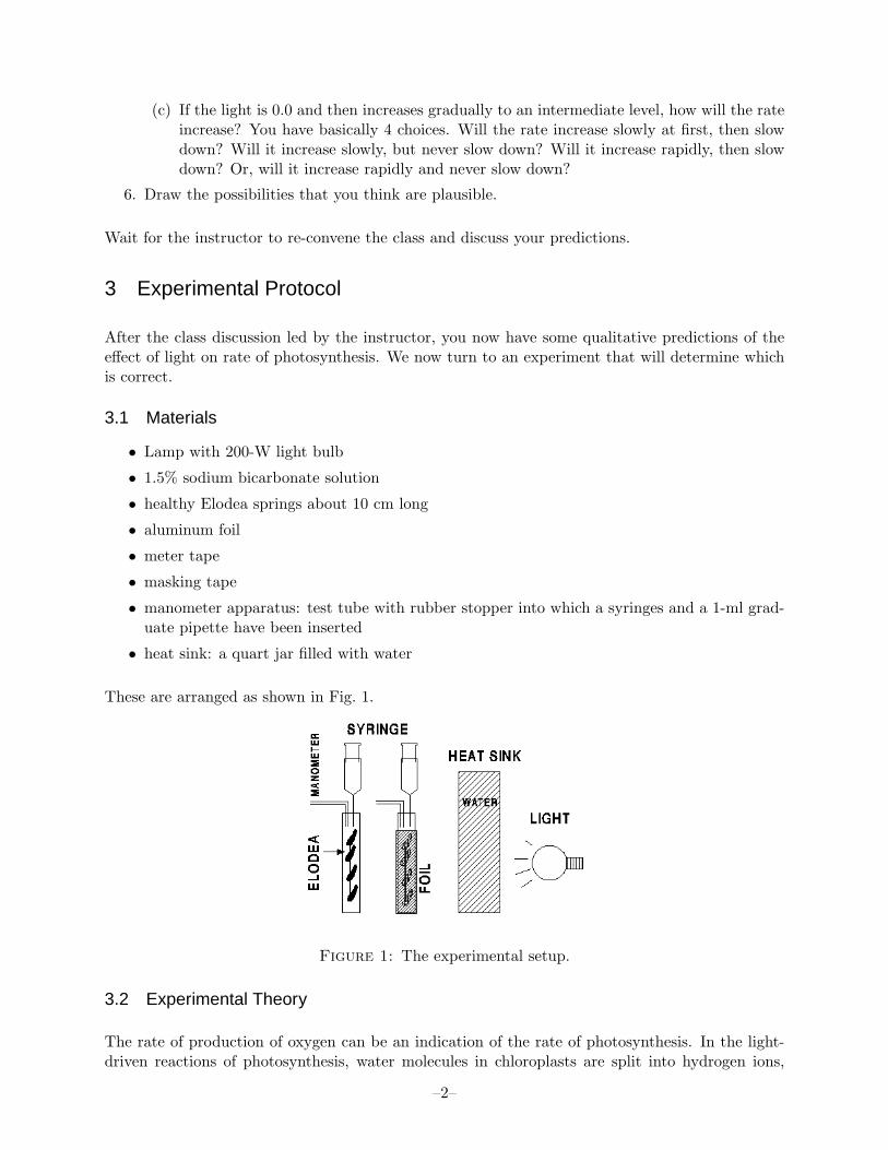
• manometer apparatus: test tube with rubber stopper into which a syringes and a 1-ml grad-uate pipette have been inserted

• heat sink: a quart jar filled with water

These are arranged as shown in Fig. 1.

Figure 1: The experimental setup.

3.2 Experimental Theory

The rate of production of oxygen can be an indication of the rate of photosynthesis. In the light-driven reactions of photosynthesis, water molecules in chloroplasts are split into hydrogen ions,

–2–

electrons, and oxygen. The oxygen produced collects in the plant tissue and passes out of thestomata into the medium surrounding the plant. The rate of oxygen production can thereforebe used as a test to determine the rate of photosynthesis for a particular plant in different lightintensities.

If asked to investigate the effect of light intensity on rate of photosynthesis, you might immediatelyhypothesize that increasing light intensity would increase photosynthetic rate. However, additionalstudy might lead you to modify this hypothesis. For example, certain plants have adapted toconditions of low light intensity, such as are found on a forest floor or in a highly productive lake.

You will work in teams of four students and investigate this question by varying the intensity oflight by moving a light source closer to a plant at 15 cm increments. The plant being investigatedis Elodea, an aquatic plant often found in eutrophic lakes and ponds.

3.3 Procedure

1. Assemble the manometer using Figure 1 as a guide. Fill two test tubes completely with 1.5%sodium bicarbonate. Take a piece of Elodea, make a fresh cut at the cut end, and holdingthe test tube over the sink, add the Elodea, stem end up, and the rubber stopper with thesyringe and graduated pipette to each tube. The stoppers should displace the water so thatno air is inside the tubes. Cover one tube with aluminumMini-Quiz question: what is the purpose of the covered tube?

2. Set the assembled manometers into a glass beaker or test tube rack.

3. Fill the heat sink with cold tap water and place it immediately adjacent to the manometer.

4. Using the meter tape, measure and place pieces of tape on the lab bench adjacent to the heatsink (0 cm) and 15, 30 and 45 cm away.

5. Place the plant at the 45 cm mark.

6. Use the syringe in the stopper to set the starting point of the water at a mark on the graduatedpipette close to each test tube, the experimental and the control. Record on Data Table 1(Fig. 2) the initial pipette reading. Turn off the room lights.

7. Turn on the 200 W light. Wait 15 minutes. Record in Data Table 1 the final pipette reading(F) for each tube.

8. Using the syringe, readjust the starting point of the water to a mark close to each test tubeand record the initial reading.

9. Move the light 15 cm close to the test tubes (the 30 cm mark) . Wait 15 minutes and recordin Data Table 1 the final pipette reading.

10. Continue to take readings after 15 minutes at the 15-cm and 0-cm marks, readjusting thelevel of water in the pipette and recording each initial and final reading in Data Table 1.These data will be used to calculate the photosynthesis curve

3.4 Results

1. Calculate the change in manometer reading for the control and experimental tubes by sub-tracting the final reading from the initial reading (I - F). Record your results in table 1 foreach distance.

2. Calculate the corrected volume of oxygen produced at each light intensity by subtracting thechange in the control tube (A) from the change in the experimental tube (B). Record your

–3–

Figure 2: Data Table 1

results in table 1.

3. Record in Data Table 2 (Fig. 3) the volume of oxygen produced as measured by other teams.Calculate the total and mean for the class data.

4. Plot the class data on the graph paper in Figure 4.

4 Comparing Data and Qualitative Predictions

Now you have been able to compare your data with your predictions. Is the plot of data the sameas any of the curves you guessed? If some are similar, how do they differ?

4.1 Your Job

Now we need an equation that describes our data. We want a fairly simple equation that willapproximate our results, not a complicated one that will pass through every datum. This is theart of writing equations: simple, but not too simple.

Here are some steps to help think about your data and equations.

1. Idealize your data by drawing a smooth curve that comes pretty close to all of the points.

(a) Remember, you are going to have write an equation for this curve, so don’t make yourcurve wiggle around all over the place.

–4–

Figure 3: Data Table 2

(b) On the other hand, your data are probably not a straight line, so a really simple equationlike y = mx + b won’t approximate your data very closely.]

2. Does your curve go up to a maximum and level off?

3. If it has a maximum, try drawing a horizontal line parallel to the x-axis that represents themaximum. Now, how does the curve approach the maximum? Gradually, or very abruptly?

4. If the approach is gradual, look at the difference between the maximum. Does the curve ofthe difference look like any simple functions you’ve worked with in this class or in earliermath classes? Take a chance and guess an equation. Use your calculator to see if it works.

5. Your equation didn’t work? That’s okay, try again after considering this hint:You might describe your equation verbablly this way: The DIFFERENCE is large at first(small light levels) then gets smaller and smaller.We used the same words last week to describe how light changed with depth. What equationdid we use then? Try to write mathematically something like thisDIFFERENCE = MAXIMUM - y = last week’s equationwhere now ”y” is the photosynthesis rates found in this week’s experiment.What is the ”x” in this equation?

–5–

Figure 4: Graph paper

–6–

6. If you have it figured out, write it out nicely defining all the terms.

7. If you are still having difficulties, wait for the class to re-convene and ask some questions.

5 An Equation

This material will be presented by the Instructor.

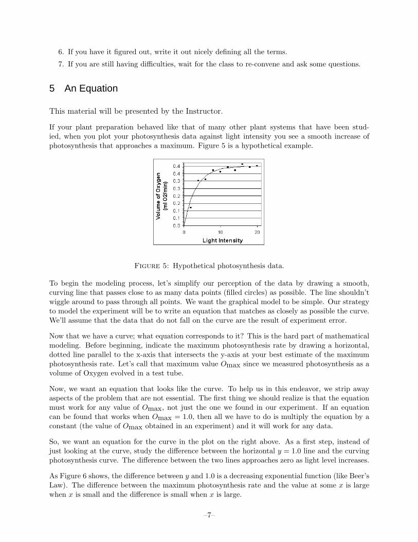
If your plant preparation behaved like that of many other plant systems that have been stud-ied, when you plot your photosynthesis data against light intensity you see a smooth increase ofphotosynthesis that approaches a maximum. Figure 5 is a hypothetical example.

Figure 5: Hypothetical photosynthesis data.

To begin the modeling process, let’s simplify our perception of the data by drawing a smooth,curving line that passes close to as many data points (filled circles) as possible. The line shouldn’twiggle around to pass through all points. We want the graphical model to be simple. Our strategyto model the experiment will be to write an equation that matches as closely as possible the curve.We’ll assume that the data that do not fall on the curve are the result of experiment error.

Now that we have a curve; what equation corresponds to it? This is the hard part of mathematicalmodeling. Before beginning, indicate the maximum photosynthesis rate by drawing a horizontal,dotted line parallel to the x-axis that intersects the y-axis at your best estimate of the maximumphotosynthesis rate. Let’s call that maximum value Omax since we measured photosynthesis as avolume of Oxygen evolved in a test tube.

Now, we want an equation that looks like the curve. To help us in this endeavor, we strip awayaspects of the problem that are not essential. The first thing we should realize is that the equationmust work for any value of Omax, not just the one we found in our experiment. If an equationcan be found that works when Omax = 1.0, then all we have to do is multiply the equation by aconstant (the value of Omax obtained in an experiment) and it will work for any data.

So, we want an equation for the curve in the plot on the right above. As a first step, instead ofjust looking at the curve, study the difference between the horizontal y = 1.0 line and the curvingphotosynthesis curve. The difference between the two lines approaches zero as light level increases.

As Figure 6 shows, the difference between y and 1.0 is a decreasing exponential function (like Beer’sLaw). The difference between the maximum photosynthesis rate and the value at some x is largewhen x is small and the difference is small when x is large.

–7–

Figure 6: Hypothetical photosynthesis data.

Your instructor will give you an equation to copy here:

Equation for Curve

which describes Fig. 6. In the last equation above, b is an empirically determined shape coefficient.When b is large the curve rises steeply; the curve has a gentle rise when b is small.

The last step to get an equation to fit to our oxygen data is to scale y so that it has units ofphotosynthesis (ml Oxygen/ml water/15min) and so that at very high light intensity we get ourobserved maximum (not 1.0). To achieve this, all we have to do is multiply our function by Omaxto get the final model:

Oxygen Equation

where O is photosynthesis as volume of Oxygen, I is light intensity, and b is an empirical shapecoefficient.

Mini-quiz: #1: Does this equation make sense? I.e., does it equal zero when light intensity iszero? Does it equal the maximum photosynthesis when light levels are very high? Plug-in somenumbers for light levels and check that the answer is yes.

Mini-quiz #2: Is it reasonable to hypothesize or assume that when light is high, photosynthesisrate will level-off at a maximum? Could photosynthesis rate decline with very high light levels?If you answered yes, does this mean our current equation is wrong?

Mini-quiz #3: Recall our arguments last week against the polynomial model for light extinctionwith depth: the model could produce physically non-sensical answers. Can the current modelproduce any of those same non-sensical values?

–8–

When the instructor is certain all the students understand this equation, he or she will ask youto proceed to the next section to discover a method to estimate the parameter b

6 Estimating b

Assume that Omax is known. Transform the equation for photosynthesis to get a linear equationfrom which you can estimate b. Work with your lab bench group to do the required algebra.

7 Analyze the Data and Estimate b

Now that we have an equation, we have to fit it to our particular data. We will use the same logicwe used in estimating the constant in Beer’s law: i.e., by taking logarithms to create a straight linefrom which we can estimate the slope. Here’s the logic:

First, isolate e−bI by itself on one side of the equals sign.

Next, take the natural log of both sides:

Finally, apply the laws of the natural logs:

And re-arrange to make this look like an equation for straight line:

As hard as it may be to believe, this is an equation for a straight line.

Make sure you see why it is a straight line. Do not be afraid to ask your instructor to make it clear.Other students will be having the same difficulties, so that by asking you will be helping them aswell.

–9–

Unfortunately, Omax occurs on both sides of the equation, but we can not simplify this any further.So, in order to plot our data to get an estimate for b as the slope of a straight line, we will need anindependent estimate of Omax.

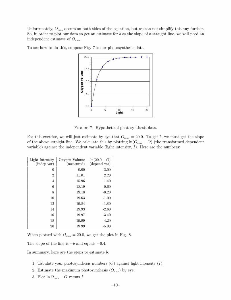
To see how to do this, suppose Fig. 7 is our photosynthesis data.

Figure 7: Hypothetical photosynthesis data.

For this exercise, we will just estimate by eye that Omax = 20.0. To get b, we must get the slopeof the above straight line. We calculate this by plotting ln(Omax −O) (the transformed dependentvariable) against the independent variable (light intensity, I). Here are the numbers:

Light Intensity Oxygen Volume ln(20.0−O)(indep var) (measured) (depend var)

0 0.00 3.002 11.01 2.204 15.96 1.406 18.19 0.608 19.18 -0.20

10 19.63 -1.0012 19.84 -1.8014 19.93 -2.6016 19.97 -3.4018 19.99 -4.2020 19.99 -5.00

When plotted with Omax = 20.0, we get the plot in Fig. 8.

The slope of the line is −b and equals −0.4.

In summary, here are the steps to estimate b.

1. Tabulate your photosynthesis numbers (O) against light intensity (I).

2. Estimate the maximum photosynthesis (Omax) by eye.

3. Plot ln Omax −O versus I.

–10–

Figure 8: Log of oxygen.

4. The slope of the line is −b

Using the empty table below, apply this technique to your data. When done, write out the completephotosynthesis equation with the correct numbers substituted for Omax and b.

Light Intensity Oxygen Volume ln(Omax −O)

(indep var) (measured) (depend var)

Using graph paper, make a plot like Fig. 8 above.

This completes the number crunching needed to analyze your experiment. The next problem is tocalculate the total amount of photosynthesis in an entire lake.

–11–

8 Estimating Photosynthesis in a Lake

Let’s review what we know:

1. We have an equation for the extinction of light in water.

2. We have an equation for the effect of light on photosynthesis.

Now we must put these together to estimate the total photosynthesis for an entire lake. We willassume a rectangular lake that has given width (”W”), length (”L”), and depth (”D”).

8.1 Your Job

Your job is to devise a plan that to calculate the total photosynthesis in the lake. You know thefollowing:

1. The light extinction equation and coefficient

2. The photosynthesis equation and coefficients: Omax and b

3. The dimensions of the lake

The task can be done in 3-4 steps. Write them down on a piece of paper.

1.

2.

3.

4.

9 Procedure to Estimate Lake Photosynthesis

Problem Statement

The only problem now is how to combine the two equations for a given lake. Suppose the lake isa rectangle with vertical sides and is 10 m deep. The area of the lake is 1,000 square meters. Wehave gone out onto the lake, dropped light meters over the side and measured light levels at eachmeter to get the data plotted as the Fig. 9.

After analyzing these data, we find that the light extinction coefficient in the Beer-Lambert lawis a = 0.5, and the light intensity at the surface is Io = 60 µmole/m2/sec. In the laboratory, Wehave performed photosynthesis experiments and obtained the estimate b = 0.4 and Omax = 0.5 mlO2/test tube/15 min. (Data in Figure 10.)

(Numbers obtained in class will differ from these.)

We want to know: How much photosynthesis occurs in one hour in the entire lake?

–12–

Figure 9: Extinction of light in a lake.

Figure 10: Photosynthesis data

Solution

We will divide the lake into 1000 columns of water each having surface area of 1 m2. Each columnwill be divided into 10 one-meter segments, corresponding to 1 m depth intervals. For each segment,we will calculate the photosynthesis in one hour, which will vary over depth because the light levelsdecrease with depth. This will give photosynthesis for a volume of 1 m3. When we add all thesegments together we will get the total photosynthesis for the entire column. Then we add thephotosynthesis for all the columns to get the value for the entire lake.

Here is a summary of the steps:

1. Calculate I (light intensity) at each depth in the column.

2. Calculate O (photosynthesis rate measured as oxygen evolved) at each depth in the columnafter converting to m3 and 1 hour.

3. Add the Os for each segment to get the column total.

4. Multiply by the lake area.

Here are the calculations for the example above. First, the conversion of experimental results intesttube units to lake units. Assume the volume of the experimental testtube was 20 ml.

Omax

m3 · hour=

Omax obsrvdtesttube vol · exper.duration

· testtube volliter

· literm3

· exp. durationhour

–13–

Using the numbers supplied:

Omax = 0.5 · 50 · 1000 · 4 = 100, 000 ml/m3/hr

where

Observed maximum O/testtube/15 min = 0.5

Testtube volumes per liter = 1000/20 = 50

Liters per cubic meter = 1000

Experimental periods per hour = 60/15 = 4

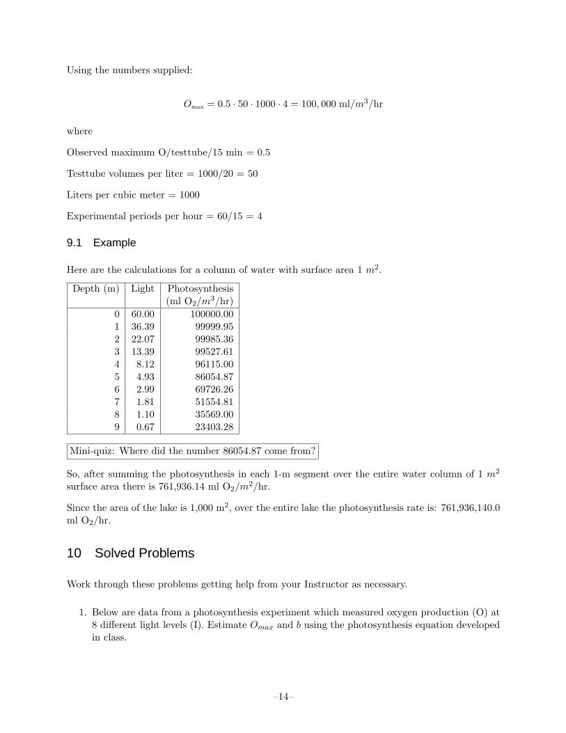
9.1 Example

Here are the calculations for a column of water with surface area 1 m2.

Depth (m) Light Photosynthesis(ml O2/m3/hr)

0 60.00 100000.001 36.39 99999.952 22.07 99985.363 13.39 99527.614 8.12 96115.005 4.93 86054.876 2.99 69726.267 1.81 51554.818 1.10 35569.009 0.67 23403.28

Mini-quiz: Where did the number 86054.87 come from?

So, after summing the photosynthesis in each 1-m segment over the entire water column of 1 m2

surface area there is 761,936.14 ml O2/m2/hr.

Since the area of the lake is 1,000 m2, over the entire lake the photosynthesis rate is: 761,936,140.0ml O2/hr.

10 Solved Problems

Work through these problems getting help from your Instructor as necessary.

1. Below are data from a photosynthesis experiment which measured oxygen production (O) at8 different light levels (I). Estimate Omax and b using the photosynthesis equation developedin class.

–14–

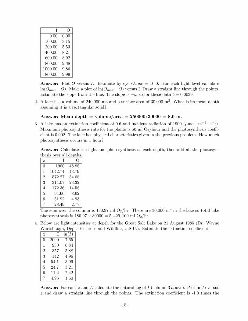
I O0.00 0.00

100.00 3.15200.00 5.53400.00 8.21600.00 8.92800.00 9.38

1000.00 9.861800.00 9.99

Answer: Plot O versus I. Estimate by eye Omax = 10.0. For each light level calculateln(Omax−O). Make a plot of ln(Omax−O) versus I. Draw a straight line through the points.Estimate the slope from the line. The slope is −b, so for these data b = 0.0039.

2. A lake has a volume of 240,000 m3 and a surface area of 30,000 m2. What is its mean depthassuming it is a rectangular solid?

Answer: Mean depth = volume/area = 250000/30000 = 8.0 m.

3. A lake has an extinction coefficient of 0.6 and incident radiation of 1900 (µmol · m−2 · s−1).Maximum photosynthesis rate for the plants is 50 ml O2/hour and the photosynthesis coeffi-cient is 0.002. The lake has physical characteristics given in the previous problem. How muchphotosynthesis occurs in 1 hour?

Answer: Calculate the light and photosynthesis at each depth, then add all the photosyn-thesis over all depths.z I O0 1900 48.881 1042.74 43.792 572.27 34.083 314.07 23.324 172.36 14.585 94.60 8.626 51.92 4.937 28.49 2.77

The sum over the column is 180.97 ml O2/hr. There are 30,000 m2 in the lake so total lakephotosynthesis is 180.97× 30000 = 5, 429, 100 ml O2/hr.

4. Below are light intensities at depth for the Great Salt Lake on 21 August 1985 (Dr. WayneWurtsbaugh, Dept. Fisheries and Wildlife, U.S.U.). Estimate the extinction coefficient.z I ln(I)0 2090 7.651 930 6.842 357 5.883 142 4.964 54.1 3.995 24.7 3.216 11.2 2.427 4.96 1.60

Answer: For each z and I, calculate the natural log of I (column 3 above). Plot ln(I) versusz and draw a straight line through the points. The extinction coefficient is -1.0 times the

–15–

slope.For these data, the Great Salt Lake extinction coefficient is 0.873.

5. How much photosynthesis occurred in the GSL in 1 hour on 21 August 1985? Assume themaximum photosynthesis rate is 75 ml O2/hr, and the photosynthesis coefficient is 0.004.The GSL has an average surface area of 1,034,000 acres and a volume of 15,390,000 acre-feet(an acre-foot is the volume of a rectangular solid 1 foot high and 1 acre in area).

Answer: Calculate the photosynthesis at each depth (O) given the light levels computedabove:z I O0 2090 74.981 930 73.182 357 57.023 142 32.504 54.1 14.595 24.7 7.066 11.2 3.297 4.96 1.47

Since we are averaging over the entire lake, we sum the photosynthesis only to the averagedepth. The area is 1, 034, 000 acres × 4.0473 = 4, 184, 598, 000 m2. The volume of GSL is15, 390, 000acre-feet × 1234.335 = 1.8996 × 1010 m3. (Work out this conversion constant foryourself.)So, the average depth is volume divided by area and equals 4.54 m.Call it 5 m and sum the photosynthesis from z = 0 to z = 4. The total column photosynthesisrate is 252.28 ml O2/hr/m2. To get the whole lake rate multiply by the area in m2 to get1.05569× 1012 ml O2/hr.

11 Homework Problems

These problems will be distributed in class and will be due on the date given by the Instructor.

–16–