Maria Peressi �Universita’ di Trieste - Dipartimento di Fisica �

Sede di Miramare (Strada Costiera 11, Trieste) �

e-mail: peressi@ts.infn.it �

tel: +39 040 2240242 �

http://www-dft.ts.infn.it/̃peressi/comp-phys.html�

Laboratory of Computational Physics�

Introduction�

M. Peressi - UniTS - Laurea Magistrale in Physics�Laboratory of Computational Physics - Unit I - part I �

(1) Computational Physics: �

- Simulations and “what-if” experiments�

- Deterministic and stochastic approaches�

-  A few examples�

(2) Courses concerning Computational Physics at UniTS (this course and the others)�

(3) Further details about this course�

(1) Computational Physics�

Computers in physics �

•  control of instruments, data collection and analysis �

• visualization �

• symbolic manipulation �

• . . . �

"……�

• numerical analysis: to solve equations which could not be tackled by analytical methods. This allows to measure theories, in a similar way as natural phenomena are measured by experiments, the ultimate goal of science being the insight and understanding gained from the comparison of these two kinds of measures. �

• simulations: to model and study physical phenomena with numerical techniques. This means doing virtual experiments in which our representation of the physical reality, though necessarily schematic and simplified, can be tuned and varied at will. �

The birth of �computational physics�

PROBLEM: Fermi-Pasta-Ulam-Tsingou 1955���

a long chain of N particles linked by springs�(one-dimensional analogue of atoms in a crystal)�

����

Linear interaction (Hooke’s law): �analytical solution �

�The energy given to a single 'normal' mode �

always remains in that mode.�

216 American Scientist, Volume 97 © 2009 Sigma Xi, The Scientific Research Society. Reproduction with permission only. Contact perms@amsci.org.

This notion of sharing energy even-ly among different modes of motion is fundamental. This precept, known as the equipartition theorem of statistical mechanics, can be extended to include molecules that are more complicated than billiard-ball-like helium, which can partition energy in rotational or vibrational movements as well. Ap-

plication of the equipartition theorem allows physicists to calculate such things as the heat capacity of a gas from basic theory.

FPU’s premise was that they could start their system off with the masses in just one simple mode of oscillation. If the system had linear springs (and no damping forces), that one mode would continue indefinitely. With nonlinear springs, however, different modes of oscillation can become excited. FPU ex-pected, the system would “thermalize” over time: The vibrating masses would partition their energy equally among all the different modes of oscillation that were possible for this system.

Visualizing the possible modes of os-cillation is a little tricky for FPU’s string of masses, but it’s easy to see how differ-ent modes of vibration arise in, for exam-ple, a plucked violin string. One mode corresponds to the fundamental tone, in which the string shifts up and down the most at the center and progressively less as you approach its fixed ends. Another mode is the first harmonic (an octave higher), in which one half of the string moves up while the other moves down, and so forth. A vibrating string has an infinite number of modes, but FPU’s system has a finite number (equal to the number of masses present).

To conduct their study, FPU (along with Mary Tsingou, who, although not an author on the report, contributed significantly to the effort) considered different numbers of masses (16, 32 or 64) in their computational experi-ments. They then numerically solved the coupled nonlinear equations that govern the motion of the masses. (They could easily derive these equa-tions from their nonlinear spring func-tion and Newton’s famous law f = ma.) In this way, FPU used the MANIAC to compute the behavior for times corre-sponding to many periods of the fun-damental mode in which they started the system. They were absolutely as-tonished by the results.

Initially, energy was shared among several different modes. After more (simulated) time elapsed, their system returned to something that resembled its starting state. Indeed, 97 percent of the energy in the system was even-tually restored to the mode they had initially set up. It was as if the billiard balls had magically reassembled from their scattered state to the perfect ini-tial triangle!

Of course, not everybody was con-vinced by these computations. One popular conjecture was that FPU had not run the simulations long enough—or perhaps the time required to achieve equipartition for the FPU system was simply too long to be observed numeri-cally. However, in 1972 Los Alamos physicist James L. Tuck and Tsingou (who at that point was using her mar-ried name, Menzel) put these doubts to rest with extremely arduous numerical simulations that found recurrences on such amazingly long time scales that they have sometimes been dubbed “su-perrecurrences.” This research made it clear that equipartition of energy wasn’t hidden from FPU by computer simula-tions that were too short—something more interesting was indeed afoot.

1 + 1 = 3Why did FPU think that nonlinear springs would ensure an equipartition of energy in their experiment? And what is this strange concept of non-linearity anyway? Obviously, the term refers to a departure from linearity, which we’ve discussed thus far only in terms of the proportionality of inputs and outputs.

Students of physics study linear systems in introductory classes be-cause they are much easier to analyze and understand. When a mass is con-nected to a linear spring and given a shove, its subsequent behavior is very simple: It will oscillate back and forth at the system’s resonant frequency, which depends only on the size of the

Figure 2. Fermi, Pasta and Ulam modeled a series of masses connected to one another by springs. The masses move back and forth according to Newton’s law of motion f = ma (force equals mass times acceleration) along the line that connects them. Here the relevant forces are the restoring forces applied by the springs. What made the study so novel and fascinating is that the restoring forces were related nonlinearly to the amount of spring compression or extension.

Figure 3. Fermi, Pasta and Ulam expected the energy in their mass-spring system eventually to become shared equally between different modes of motion, which are analogous to the modes of vibration of a plucked violin string. The fundamental mode of vibration for such a string (purple) corresponds to the note that is heard. Higher-frequency vibrational modes give rise to various harmonics of that note. The motions shown here correspond to the second (pink), third (green), fourth (blue) and fifth (orange) harmonics.

The birth of �computational physics�

PROBLEM: Fermi-Pasta-Ulam-Tsingou 1955���

in presence of a weak non linear coupling (quadratic or cubic correction to the linear term),

which modes will be excited after a long enough time? �

�Expected behavior based on the equipartition theorem: the energy will be equally distributed among all the

degrees of freedom of the system.�However: analytical solution impossible�

216 American Scientist, Volume 97 © 2009 Sigma Xi, The Scientific Research Society. Reproduction with permission only. Contact perms@amsci.org.

This notion of sharing energy even-ly among different modes of motion is fundamental. This precept, known as the equipartition theorem of statistical mechanics, can be extended to include molecules that are more complicated than billiard-ball-like helium, which can partition energy in rotational or vibrational movements as well. Ap-

plication of the equipartition theorem allows physicists to calculate such things as the heat capacity of a gas from basic theory.

FPU’s premise was that they could start their system off with the masses in just one simple mode of oscillation. If the system had linear springs (and no damping forces), that one mode would continue indefinitely. With nonlinear springs, however, different modes of oscillation can become excited. FPU ex-pected, the system would “thermalize” over time: The vibrating masses would partition their energy equally among all the different modes of oscillation that were possible for this system.

Visualizing the possible modes of os-cillation is a little tricky for FPU’s string of masses, but it’s easy to see how differ-ent modes of vibration arise in, for exam-ple, a plucked violin string. One mode corresponds to the fundamental tone, in which the string shifts up and down the most at the center and progressively less as you approach its fixed ends. Another mode is the first harmonic (an octave higher), in which one half of the string moves up while the other moves down, and so forth. A vibrating string has an infinite number of modes, but FPU’s system has a finite number (equal to the number of masses present).

To conduct their study, FPU (along with Mary Tsingou, who, although not an author on the report, contributed significantly to the effort) considered different numbers of masses (16, 32 or 64) in their computational experi-ments. They then numerically solved the coupled nonlinear equations that govern the motion of the masses. (They could easily derive these equa-tions from their nonlinear spring func-tion and Newton’s famous law f = ma.) In this way, FPU used the MANIAC to compute the behavior for times corre-sponding to many periods of the fun-damental mode in which they started the system. They were absolutely as-tonished by the results.

Initially, energy was shared among several different modes. After more (simulated) time elapsed, their system returned to something that resembled its starting state. Indeed, 97 percent of the energy in the system was even-tually restored to the mode they had initially set up. It was as if the billiard balls had magically reassembled from their scattered state to the perfect ini-tial triangle!

Of course, not everybody was con-vinced by these computations. One popular conjecture was that FPU had not run the simulations long enough—or perhaps the time required to achieve equipartition for the FPU system was simply too long to be observed numeri-cally. However, in 1972 Los Alamos physicist James L. Tuck and Tsingou (who at that point was using her mar-ried name, Menzel) put these doubts to rest with extremely arduous numerical simulations that found recurrences on such amazingly long time scales that they have sometimes been dubbed “su-perrecurrences.” This research made it clear that equipartition of energy wasn’t hidden from FPU by computer simula-tions that were too short—something more interesting was indeed afoot.

1 + 1 = 3Why did FPU think that nonlinear springs would ensure an equipartition of energy in their experiment? And what is this strange concept of non-linearity anyway? Obviously, the term refers to a departure from linearity, which we’ve discussed thus far only in terms of the proportionality of inputs and outputs.

Students of physics study linear systems in introductory classes be-cause they are much easier to analyze and understand. When a mass is con-nected to a linear spring and given a shove, its subsequent behavior is very simple: It will oscillate back and forth at the system’s resonant frequency, which depends only on the size of the

Figure 2. Fermi, Pasta and Ulam modeled a series of masses connected to one another by springs. The masses move back and forth according to Newton’s law of motion f = ma (force equals mass times acceleration) along the line that connects them. Here the relevant forces are the restoring forces applied by the springs. What made the study so novel and fascinating is that the restoring forces were related nonlinearly to the amount of spring compression or extension.

Figure 3. Fermi, Pasta and Ulam expected the energy in their mass-spring system eventually to become shared equally between different modes of motion, which are analogous to the modes of vibration of a plucked violin string. The fundamental mode of vibration for such a string (purple) corresponds to the note that is heard. Higher-frequency vibrational modes give rise to various harmonics of that note. The motions shown here correspond to the second (pink), third (green), fourth (blue) and fifth (orange) harmonics.

The birth of �computational physics�

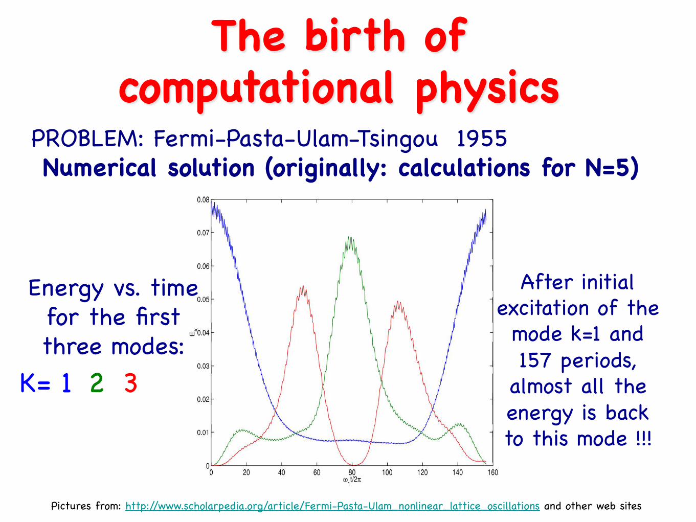
PROBLEM: Fermi-Pasta-Ulam-Tsingou 1955�Numerical solution (originally: calculations for N=5) �

Pictures from: http://www.scholarpedia.org/article/Fermi-Pasta-Ulam_nonlinear_lattice_oscillations and other web sites �

After initial excitation of the mode k=1 and 157 periods,

almost all the energy is back to this mode !!! �

Energy vs. time for the first three modes: �

K= 1 � 2� 3�

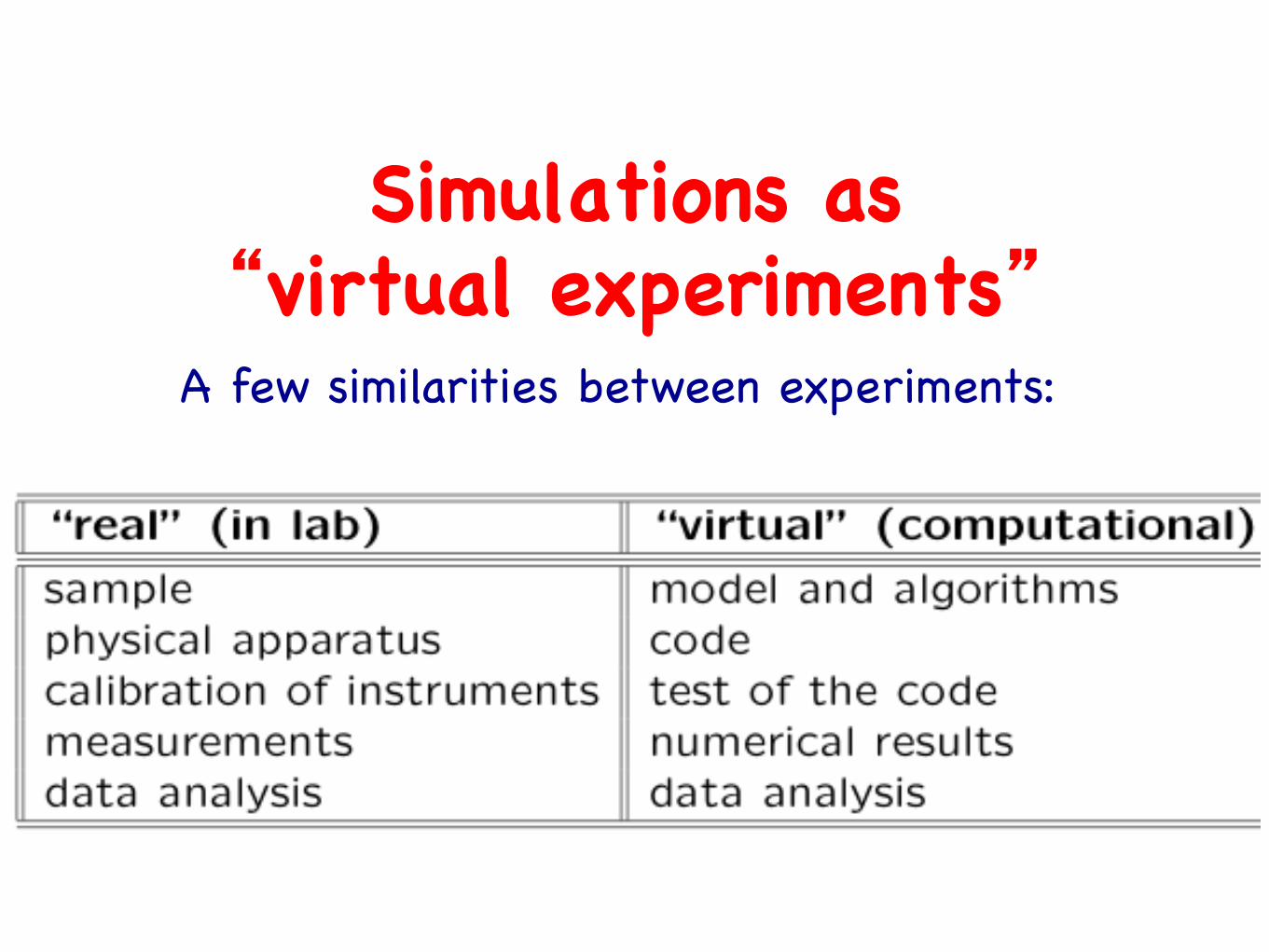
Simulations as �“virtual experiments” �

A few similarities between experiments: �

Simulations as �“virtual experiments” �

A few similarities between experiments: �

With errors!!!�

•  Importance of simulations: “what–if” experiments (large flexibility in varying parameters; e.g. material properties can be studied also under conditions not accessible in real labs) ; predictions, not just description.�

•  Use of simulations: not “final goal”, but “instruments” to study and shed light on complex phenomena and/or systems with many degrees of freedom or many variables and parameters �

•  in the last ~4 decades simulation has emerged as the third fundamental paradigm of science, beside theory and experiment �

•  “The computer is a tool for clear thinking” (Freeman J. Dyson) �

•  “. . . whose [of the calculations] purpose is insight, not numbers” (V. Hamming) �

The purposes �of the scientific calculus�

• deterministic �Info can be obtained both on the equilibrium properties and on the dynamics of the system ��• stochastic (Monte Carlo, MC) �Typically to simulate random processes, �and/or sampling of most likely events �

TWO different approaches for numerical simulations�

The deterministic approach�We can write the equations of motion �

(Classical => Newton; Quantum => Schroedinger)��

and we know the initial condition ��

the problem is related to the �numerical integration of differential equations�(or integral-differential in quantum problems)�

�(like the FPUT problem)�

�

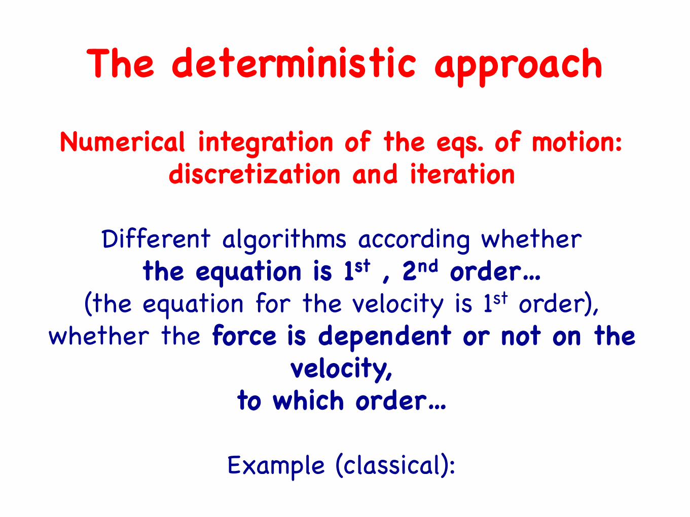
The deterministic approach�Numerical integration of the eqs. of motion: �

discretization and iteration��

Different algorithms according whether�the equation is 1st , 2nd order…�

(the equation for the velocity is 1st order), �whether the force is dependent or not on the

velocity, �to which order…�

�Example (classical): �

The deterministic approach�

x(1) v(1) F(1) � x(2) v(2) F(2)� x(3) v(3) F(3)� ... ... …�

F1�F2�

F3�F4�

Discretization of the equation of motion and iteration: �

The stochastic approach�

1) Some physical processes which are inherently probabilistic.�

2) Many large classical systems which have so many variables, or degrees of freedom, that an exact treatment is intractable and not useful. �

Useful to model:�

Probabilistic physical processes�We attempt to follow the `time dependence’ of a model for which change, or growth, does not proceed in some rigorously predefined fashion (e.g. according to Newton’s equations of motion) but rather in a stochastic manner which depends on a sequence of random numbers which is generated during the simulation.

E.g.: radioactive decay

Systems�with many degrees of freedom �

E.g.: Thermodynamic properties of gases��Impossible and not useful to know the exact positions and velocities of all molecules.��Useful properties are statistical: average energy of particles (temperature), average momentum change from collisions with walls of container (pressure), etc.��The error in the averages decreases as the number of particles increases. Macroscopic volume of gas has O(10^23) molecules. Thus a statistical approach works very well! �

Monte Carlo

Monte Carlo refers to any procedure which makes use of random numbers (*)�

Monte Carlo is used in: �- Numerical analysis �- Statistical Mechanics Simulation �

(*) a sequence of random numbers is a set of numbers which looks unpredictable but with well defined statistical properties�

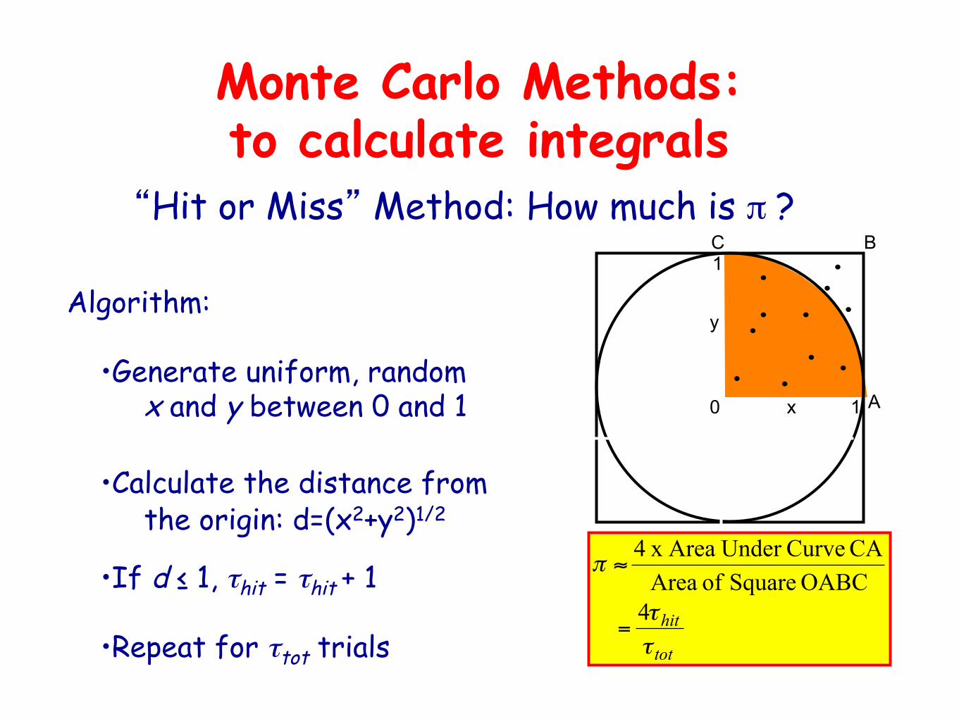
Monte Carlo Methods: to calculate integrals

“Hit or Miss” Method: Ηοw much is π ?

A 1

C B

y

x 0

1

Algorithm:

• Generate uniform, random x and y between 0 and 1 • Calculate the distance from the origin: d=(x2+y2)1/2

• If d ≤ 1, τhit = τhit + 1

• Repeat for τtot trials tot

hit

ττ

π

4

OABC Square of AreaCA Curve Under Area x 4

=

≈

.�.�.� .�

.�.�

.�

.�

.�.�.�

A few selected examples�of applications�

�(most in computational condensed matter)�

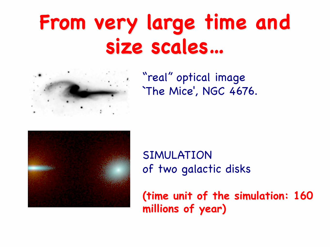
“real” optical image�`The Mice', NGC 4676. �

SIMULATION �of two galactic disks��(time unit of the simulation: 160 millions of year)

From very large time and size scales…�

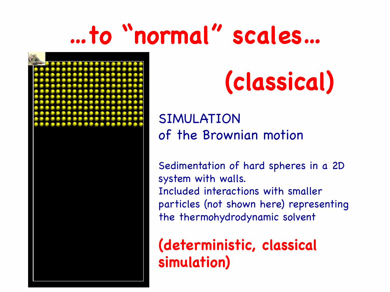
…to “normal” scales…�

SIMULATION �of the Brownian motion ��Sedimentation of hard spheres in a 2D system with walls.�Included interactions with smaller particles (not shown here) representing the thermohydrodynamic solvent ��(deterministic, classical simulation) �

(classical) �

... again colloidal systems growth on a substrate... �

REAL IMAGE (by �Atomic Field Microscopy) of a gold colloid of about 15 nm on a mica substrate�

SIMULATION �of a diffusion-limited �auto-aggregation model (fractal)�

(stochastic, classical simulation) �

… to the atomic scale �

(In collaboration �with Surf Sci �

Reactivity Group �of TASC)�

Exp Low T - �STM images�

Simulated�STM images�

Best models�

CO2@Ni(110)�

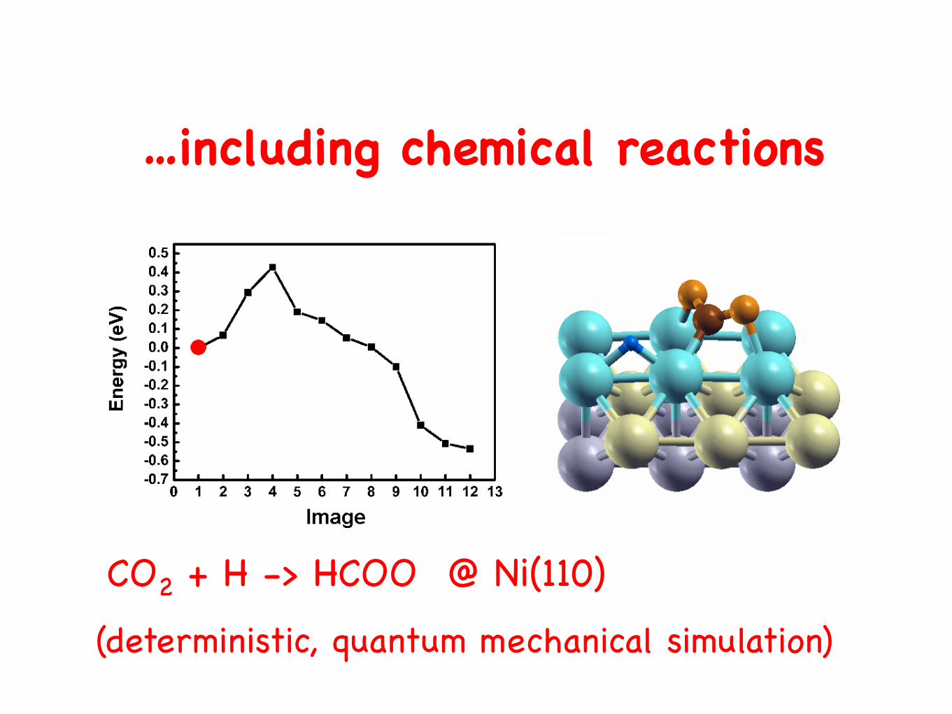
CO2 + H -> HCOO @ Ni(110)�(deterministic, quantum mechanical simulation)�

…including chemical reactions�

Computational condensed matter �• wide range of length scales: ≈12 orders of magnitude

(nuclei/electrons/atoms/chemical bonds ~ 10−12 m, fracture/macroscopic mechanical phenomena ~ 100 m; nano / micro / meso / macroscopic scales) �

• wide range of time scales: ≈12 orders of magnitude (nuclei/electrons/atoms/chemical bonds ~ 10−12 s, fracture/macroscopic mechanical phenomena ~ year)�

• wide range of chemical-physical properties: structural, elastic, vibrational, electronic, dielectric, magnetic, optical, thermal . . . �

• wide range of materials: different phases, traditional materials (crystalline / amorphous , metals/ semiconductors / insulators . . .), new materials. . . �

different kind of interactions�

•  Classic�

• Quantum �

different approaches �•  Deterministic�

•  Stochastic�

…and also different specific techniques �

corresponding to different size/time scales: �

• continuous models (for macroscopic systems) �

• atomistic simulations �

- ab - initio techniques (or “first-principles”): up to ~10^3 atoms, 10 ps �

-  Semiempirical techniques: up to 10~7 atoms, 1 ms�

-  models at different levels�

(2) Courses concerning Computational Physics at

UniTS�

This course �•  IS NOT a course on Information

Technology, Computer Science, Programming languages…�

•  BUT a PHYSICS LAB. �

•  focusing on modeling, problem solving and algorithms �

This course �•  Stochastic approach, classical interactions (mainly) �

•  + basic ingredients of the deterministic approach (Molecular Dynamics) and quantum mechanics (Variational Monte Carlo) (1 week each topic)�

This course and others in the Physics course at UniTS�

•  complementary to “Classical simulations of many body systems” (E. Smargiassi, I semester II year) (deterministic, classical)�

•  complementary to “Numerical Methods of Quantum Mechanics” (P. Giannozzi, II semester I year) (deterministic, quantum)�

(3) Further details about this course �

Web page of the course�http://www-dft.ts.infn.it/̃peressi/comp-phys.html�

�With:�

-  Important announcements�-  Detailed contents of each lecture�-  Lectures notes �-  Exercises�-  Info about textbooks �-  links, tutorials (for surviving with Linux/Unix,

Fortran90, gnuplot…)�-  Info about exams�

Use it! �

Properties and generation of Random Numbers with different distributions.･�

Monte Carlo simulation of Random Walks.･ �

Numerical integration in 1 dimension: deterministic and stocastic algorithms;･ �

Monte Carlo algorithms.･ �

Error estimate and reduction of the variance methods.･ �

Metropolis algorithm for arbitrary random number generation.･ �

Metropolis method in the canonical ensamble.･ �

Ising model and Metropolis-Monte Carlo simulation.･ �

Classical fluids: Monte Carlo and Molecular Dynamics simulation of hard spheres and Lennard-Jones fluids.･�

Microstates and macrostates: efficient algorithm for the numerical calculation of entropy.･ �

Variational Monte Carlo in quantum mechanics (basics).･ �

Lattice gas: vacancy diffusion in a solid.･ �

Caos and determinism: classical billiards and caotic billiards, logistic maps; Lyapunov exponents.･ �

Fractals: diffusion and aggregation, models for surface growth simulation. Percolation.

Available computational resources: INFIS�

http://df.units.it/?q=it/node/2919 �Or: �http://df.units.it/ => link: DIDATTICA => SERVIZI AGLI STUDENTI �

Remote connection: �$ssh username@w01.infis.units.it ��Your address at INFIS: �username@infis.univ.trieste.it �nome.cognome@infis.univ.trieste.it ��

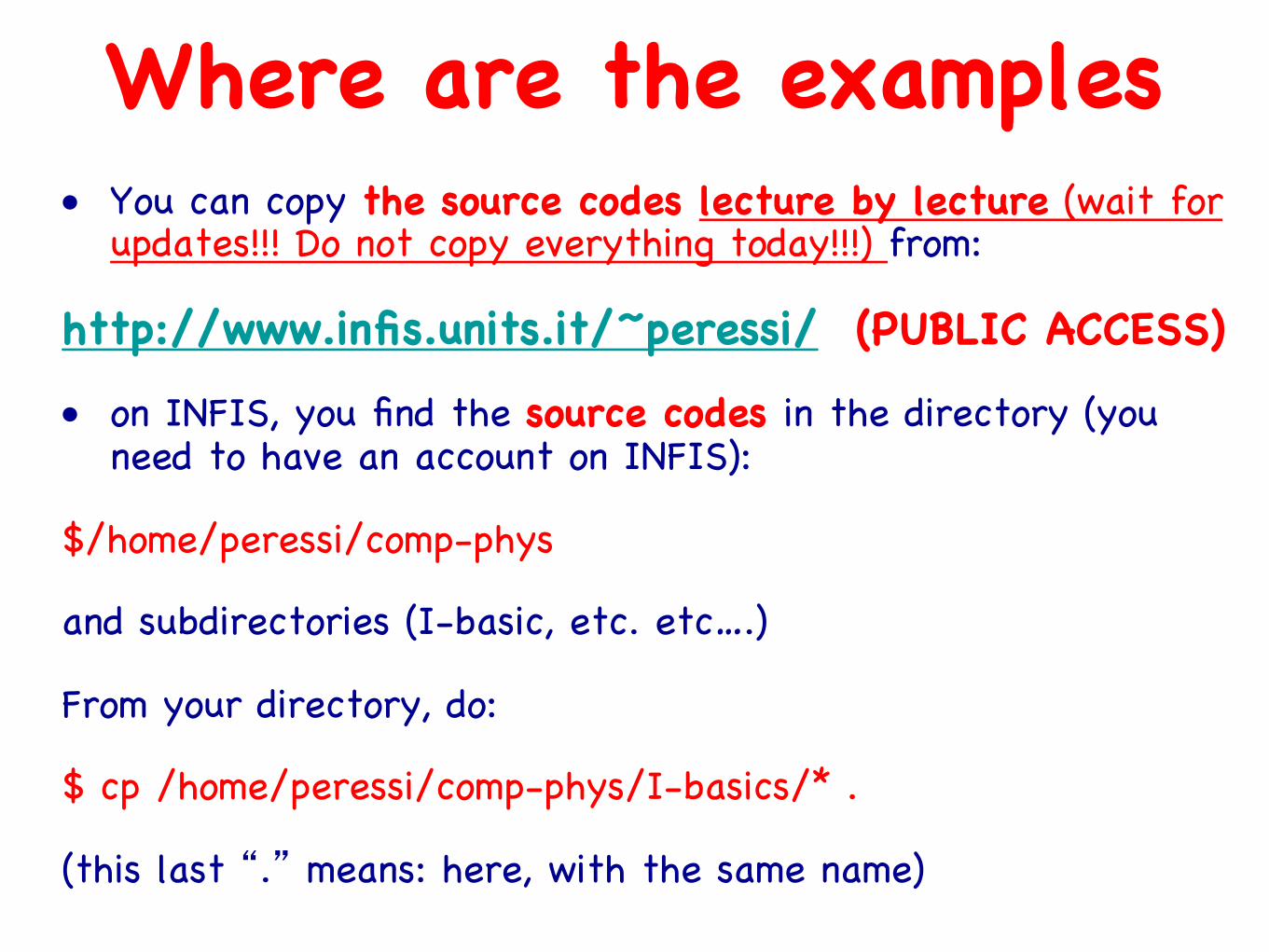
Where are the examples�•  You can copy the source codes lecture by lecture (wait for

updates!!! Do not copy everything today!!!) from: �

http://www.infis.units.it/~peressi/ (PUBLIC ACCESS) �

•  on INFIS, you find the source codes in the directory (you need to have an account on INFIS): �

$/home/peressi/comp-phys �

and subdirectories (I-basic, etc. etc….)�

From your directory, do: �

$ cp /home/peressi/comp-phys/I-basics/* .�

(this last “.” means: here, with the same name)�

�

fortran compilers on INFIS�•  g95 or gfortran (free): ([] for optional) �

$ g95 [-o test.o] test.f90 or �

$ gfortran [–std=f95] [-o test.o] test.f90 �

•  OTHERS (NOT SUPPORTED ON INFIS): �

ifort (Fortran Intel compiler, NOT free) �

F (free; useful options: -ieee=full for floating point exception manipulation)�

•  executables (e.g. test.o or a.out by default): �

$ ./a.out (or $bash a.out)�

A few useful �UNIX (Linux, MacOSx,…) commands: �

Check your space! �

$ quota �

or “du” (displays disk usage statistics): �

$ du ~ | more�

(if “-k” flag is specified, the number of 1024-byte blocks used by the file is displayed): �

$ du -k ~ | more (Last line shows the total)�

$ find . -size +20000 –print (to identify big files)�

�