laboratory investigations and field data processing
TRANSCRIPT

Lecture Series SGL 308: Introduction to Geological Mapping Lecture 5
57
LECTURE 5 LABORATORY INVESTIGATIONS AND FIELD DATA
PROCESSING
LECTURE OUTLINE
Page
5.0 Introduction 57 5.1 Objectives 58 5.2 Petrography 59
5.3 The Petrographic Microscope
5.3.1 Focusing the Microscope
5.3.2 Centering the Microscope
59 59 60
5.4 Routine of Mineral Identification
5.4.1 Form and Crystallographic Properties
5.4.2 Optical Properties
5.4.3 Relative Index and Relief
61 62 66 68
5.5 Principle of Operation of chemical and X-ray Analytical methods
5.5.1 Chemical and X-ray analysis
5.5.2 Elemental analysis of Atomic Absorption Spectroscopy (AAS)
5.5.3 Elemental analysis by X-ray Fluorescence (XRF)
5.5.4 Sodium Bisulfate Fusion
5.5.5 X-ray Diffraction
5.5.6 Electron Microscopy
5.5.7 Scanning Electron Microscopy (SEM)
5.5.8 Radiography of Rock Slabs
70 70 71 71 72 72 73 74 75
5.6 Spherical Projections
5.6.1 Rose diagrams
76 77
5.7 Thin and Polished Sections Preparation 81
5.8 Summary 82
5.9 References 83
Lecture Series SGL 308: Introduction to Geological Mapping Lecture 5
58
5.0 INTRODUCTION
Welcome to lecture 5 of this unit. The study of rocks involves many methods, the
procedures followed depending on the nature of the rock, the purpose of the study, and
the facilities and time available. In the previous lectures you broadly learned about the
basic principles of geological mapping, the methods used in locating oneself in the field,
usage of geological equipment, sampling techniques and labeling of rock samples. The
accurate mapping and description of the rocks in the field is the basic starting point of the
study of rocks. It is equally true that all conclusions or theories regarding the origin and
relationship of rocks based upon laboratory investigations must be checked in the field.
In this lecture you will be given an overview of the basic laboratory methods and data
processing techniques commonly used in the study of rocks. More specifically you will
be introduced to the basic principles of petrographic study of rocks under the microscope
and selected geochemical and X-ray analytical techniques. You are encouraged to
undertake more detailed review of the analytical techniques discussed in this lecture as
suggested at the end of this lecture in the reference section. The extra library study will
enable you to be enriched yourself with an in-depth content of the subject matter. Indeed
the detailed description of the various analytical methods and procedures are beyond the
scope of the present lecture topic. The purpose of this lecture topic is to bring to your
awareness of the analytical techniques available for your use and to stimulate your
interest to produce relevant and quality data in your research work.
5.1 OBJECTIVES
At the end of this lecture you should be able to: (a) Describe the principle of operation of the petrographic microscope.
(b) Determine the form and crystallographic properties of minerals
(c) Determine the optical properties of minerals using the petrographic microscope.
(d) Describe the principle of operation of chemical and X-ray analytical methods.
(e) Analyze and plot structural data using spherical projections.
(g) Describe the preparation of thin- and polished rock sections.

Lecture Series SGL 308: Introduction to Geological Mapping Lecture 5
59
5.2 PETROGRAPHY
Petrography is the description and classification of rocks. Following the field study and
mapping of rocks, the next step in their study is the preparation and examination of thin
sections. This procedure provides us with precise information regarding the mineralogy
of the rock, the proportions of the various minerals, and the texture – a feature that is as
important as the mineralogy. In some instances the exact identification of the minerals
may not be possible, and the thin-section examination must be supplemented by other
methods of mineral identification, for example, accurate determination of indices of
refraction, density, x-ray diffraction, or chemical tests. In certain type of investigation, it
is often desirable also to determine the chemical composition of the rock or rocks being
studied.
5.3 THE PETROGRAPHIC MICROSCOPE
The polarizing microscope is a specialized instrument designed for the study of minerals,
rocks and inorganic crystals and aggregates. It differs from the ordinary microscope in
that it is equipped with two polarizing elements and certain other accessories (for details
refer to the Mineralogy study unit SGL 201- Principles of Mineralogy by Nyamai, 2004).
5.3.1 Focusing the Microscope
In order that the microscope may be operated with minimum eye-strain, it is essential that
it be in focus for the user’s eye. The first step in focusing is to remove the eye piece from
the tube; with the eye relaxed and focused at infinity (i.e., on a distant object) the eye
piece is placed in front of the eye, and the top lens (which is adjustable in good
microscopes) is moved until the cross hairs are sharply in focus. When the eye piece is
returned to the microscope and the slide on the stage is brought into focus, there should
be no strain in examining the slide. In other words, by this procedure, the microscope,
and not the eye, does the focusing. It is also desirable, in the interests of the eye comfort,
to train the eye to observe the image in the microscope with the unused eye open.
Lecture Series SGL 308: Introduction to Geological Mapping Lecture 5
60
5.3.2 Centering the Microscope
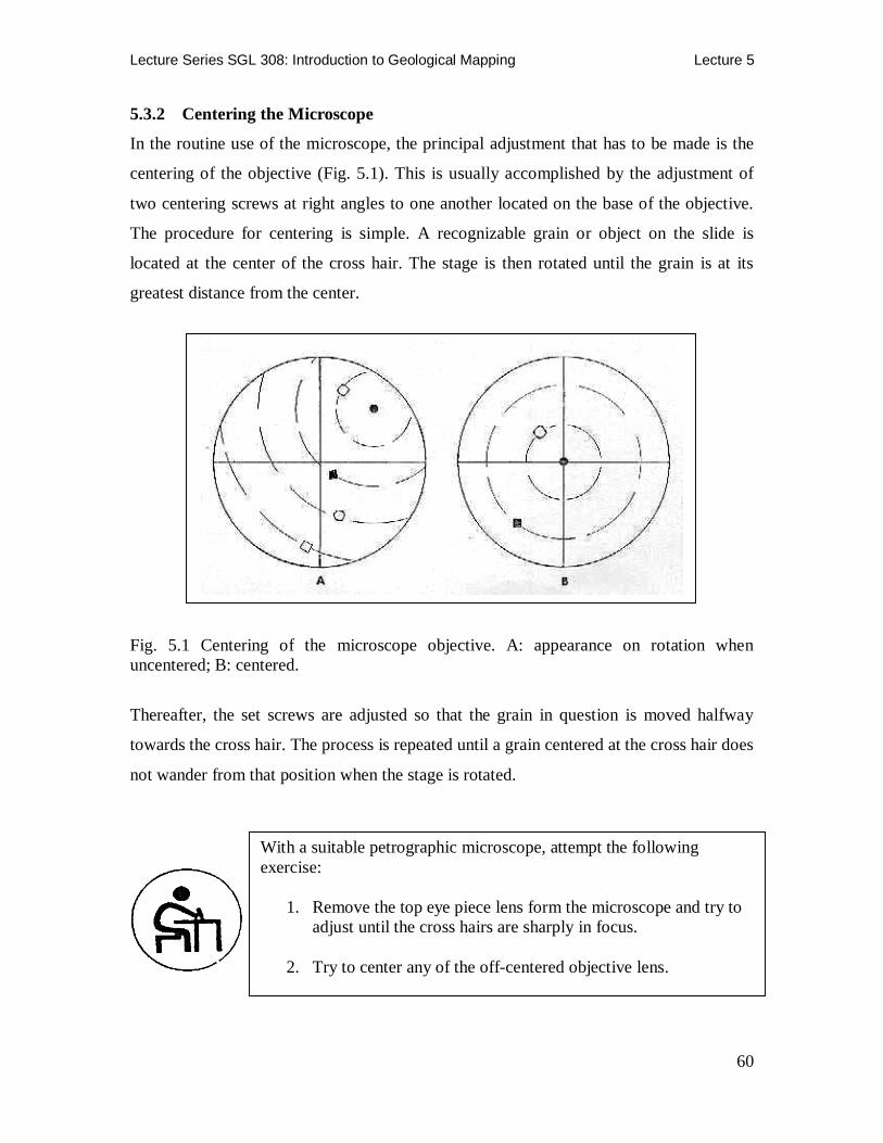
In the routine use of the microscope, the principal adjustment that has to be made is the
centering of the objective (Fig. 5.1). This is usually accomplished by the adjustment of
two centering screws at right angles to one another located on the base of the objective.
The procedure for centering is simple. A recognizable grain or object on the slide is
located at the center of the cross hair. The stage is then rotated until the grain is at its
greatest distance from the center.
Fig. 5.1 Centering of the microscope objective. A: appearance on rotation when uncentered; B: centered.
Thereafter, the set screws are adjusted so that the grain in question is moved halfway
towards the cross hair. The process is repeated until a grain centered at the cross hair does
not wander from that position when the stage is rotated.
With a suitable petrographic microscope, attempt the following exercise:
1. Remove the top eye piece lens form the microscope and try to adjust until the cross hairs are sharply in focus.
2. Try to center any of the off-centered objective lens.

Lecture Series SGL 308: Introduction to Geological Mapping Lecture 5
61
5.4 ROUTINE OF MINERAL IDENTIFICATION
In the study of rocks with the microscope, the first step is the identification of the
constituent minerals. The identification of minerals with the microscope is possible,
because a large number of physical properties, more or less independent of one another,
may be observed. The greater the number of such observations that can be made, the
greater the likelihood that each mineral will have its own distinctive characteristics. The
general sequence of observations under the microscope should take the form as tabulated
in Table 5.1.
Table 5.1 General sequence of petrographic observations under the microscope.
No. Description
1. Form and Crystallographic properties
a. Crystal form if developed b. Cleavage, parting, or fracture: number of cleavages and angular
relationships to one another, perfection of cleavage, characteristics of parting and fracture.
c. Shape of grain, if distinctive (fibrous, acicular, bladed, radiating, reticulate, tabular, platy).
d. Inclusions, intergrowths, alteration, association with other minerals.
b. Twinning. 2. Optical Properties
a. Opaque minerals: color by reflected light b. Transparent or translucent minerals
Color and pleochroism Relative index and relief
c. Examination under crossed nicols Isotropic or anisotropic In anisotropic minerals, interference colors and
determination of birefringence Extinction angle. Determination if length-slow or length fast
d. Information from interference figure Uniaxial or biaxial; sign, whether positive or negative If Biaxial; optic angle, dispersion, orientation of optic plane, determination of pleochroic formula.
Lecture Series SGL 308: Introduction to Geological Mapping Lecture 5
62
5.4.1 Form and Crystallographic Properties
5.4.1.1 Crystal Form The crystal form is very useful in the recognition of those minerals that characteristically
show well-developed faces. Examples of such minerals include pyrite, chromite, garnet,
leucite, olivine, zircon, apatite, sphene, rutile, tourmaline, and staurolite. Many minerals,
notably the amphiboles, usually exhibit a distinctive prismatic form, although they do not
commonly have terminations, so that completely closed crystal forms are not usual.
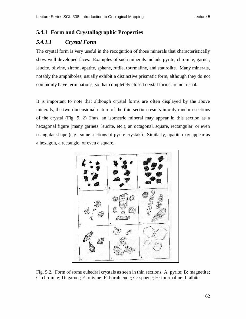
It is important to note that although crystal forms are often displayed by the above
minerals, the two-dimensional nature of the thin section results in only random sections
of the crystal (Fig. 5. 2) Thus, an isometric mineral may appear in this section as a
hexagonal figure (many garnets, leucite, etc.), an octagonal, square, rectangular, or even
triangular shape (e.g., some sections of pyrite crystals). Similarly, apatite may appear as
a hexagon, a rectangle, or even a square.
Fig. 5.2. Form of some euhedral crystals as seen in thin sections. A: pyrite; B: magnetite; C: chromite; D: garnet; E: olivine; F: hornblende; G: sphene; H: tourmaline; I: albite.

Lecture Series SGL 308: Introduction to Geological Mapping Lecture 5
63
5.4.1.2 Cleavage and Parting
Cleavage Other crystallographic characteristics, such as cleavage, are of great value in the
identification of minerals. Some minerals, such as mica, epidote, chlorite, talc, brucite,
chloritoids, sillimanite, prehnite, and topaz, exhibit only one direction of cleavage.
Others possess two; in such instances the angle between the cleavages is significant.
Hornblende has two cleavages intersecting at 56o; orthoclase, pyroxene, scapolite, and
andalusite have cleavages intersecting at right angles; those of plagioclase and microcline
intersect at a little less than 90o.
Measurement of angles between cleavages can be a useful identification technique,
particularly in the distinction between amphiboles e.g., hornblende (two cleavages at 124
degrees) and pyroxenes e.g., augite (two cleavages at nearly 90 degrees). Figure 5.3
illustrates the two characteristic cleavages.
Figure 5.3 (a) Sections normal to c-axis in augite, showing the two cleavages nearly at right angles to each other; (b) a similar section of hornblende showing cleavages at 124 degrees.
Sections not at right angles to the cleavage directions but oblique to them will show
angles smaller than the true angle. Random sections of minerals possessing two cleavage
directions may show only one. Prismatic sections of hornblende, pyroxene, andalusite,
and scapolite will show only one direction of cleavage, although in certain of these
sections focusing up and down will reveal that some of the cleavage planes dip one way,
some another.

Lecture Series SGL 308: Introduction to Geological Mapping Lecture 5
64
Parting Parting is a characteristic property of many minerals. In some minerals (e.g., pyroxene,
spinel, and corundum), it is difficult to distinguish parting from cleavage in thin section.
In other minerals, such as pyroxene (bronzite and diallage) and amphibole, it differs from
cleavage in having finite width and more definite, regular appearance, as if drawn with a
ruler on the grain showing it. It is often marked by the presence of inclusions or
alteration.
Fracturing may be a distinctive feature to aid in the identification of some minerals. Thus,
quartz may exhibit conchoidal fracturing, and olivine grains frequently are cut by curving
fractures.
5.4.1.3 Shape of Grains, Intergrowths and Inclusions
Shape of Grains The shape of grains is characteristic of certain minerals. Zeolites, such as natrolite, occur
in radiating acicular crystals; chrysotile occurs in fibrous form; serpentine is in masses of
reticulating fibers and fibrous veins; a variety of sillimanite (fibrolite) occurs in irregular
clumps of fibrous crystals; kyanite and wollastonite occur often in bladed form; prehnite
and chloritoid frequently display a bladed form with “bow-tie” structure; tabular habits
are characteristic of ilmenite crystals, tridymite, and many feldspar crystals; micas,
chlorites, talc, brucite, graphite, and clay minerals occur in platy of flaky crystals. Figure
Using the petrographic microscope, distinguish and identify grains of hornblende and pyroxene based on their distinct cleavage pattern. NB. Thin section specimens will be provided by the instructor.
What is the main difference between cleavage and parting in minerals?

Lecture Series SGL 308: Introduction to Geological Mapping Lecture 5
65
5.4 illustrates a contrast shown between well-formed tabular grains of biotite and well-
formed prismatic grains of apatite as they appear in thin section.
Figure 5.4 Shape in thin section of (a) tabular biotite contrasted with (b) prismatic apatite.
Intergrowths Intergrowths maybe of considerable value in rapid identification of some minerals.
Perthitic intergrowths are of great use in distinguishing potash feldspar from sodic
plagioclase (see Fig. 5.5).
A B
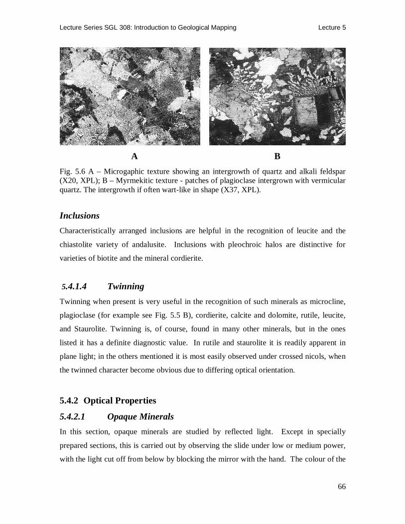
Figure 5.5 (A) -Perthitic-structure in alkali feldspar ( X 50); and in (B) - Calcic plagioclase showing characteristic broad lamellae of albite twins (X 30) Crossed nicols. Micrographic and myrmekitic intergrowths most commonly are indicative of quartz and
alkali feldspar, and quartz and plagioclase, respectively (see Fig. 5.6)
Lecture Series SGL 308: Introduction to Geological Mapping Lecture 5
66
A B
Fig. 5.6 A – Microgaphic texture showing an intergrowth of quartz and alkali feldspar (X20, XPL); B – Myrmekitic texture - patches of plagioclase intergrown with vermicular quartz. The intergrowth if often wart-like in shape (X37, XPL).
Inclusions Characteristically arranged inclusions are helpful in the recognition of leucite and the
chiastolite variety of andalusite. Inclusions with pleochroic halos are distinctive for
varieties of biotite and the mineral cordierite.
5.4.1.4 Twinning Twinning when present is very useful in the recognition of such minerals as microcline,
plagioclase (for example see Fig. 5.5 B), cordierite, calcite and dolomite, rutile, leucite,
and Staurolite. Twinning is, of course, found in many other minerals, but in the ones
listed it has a definite diagnostic value. In rutile and staurolite it is readily apparent in
plane light; in the others mentioned it is most easily observed under crossed nicols, when
the twinned character become obvious due to differing optical orientation.
5.4.2 Optical Properties
5.4.2.1 Opaque Minerals In this section, opaque minerals are studied by reflected light. Except in specially
prepared sections, this is carried out by observing the slide under low or medium power,
with the light cut off from below by blocking the mirror with the hand. The colour of the
Lecture Series SGL 308: Introduction to Geological Mapping Lecture 5
67
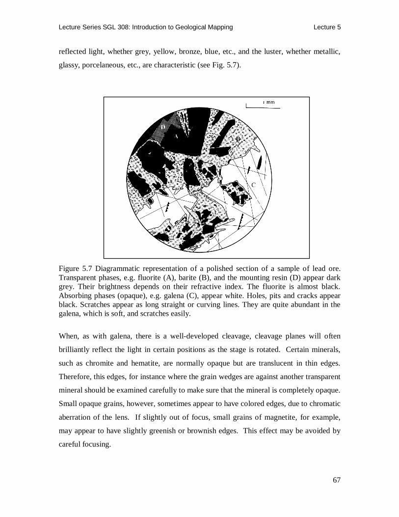
reflected light, whether grey, yellow, bronze, blue, etc., and the luster, whether metallic,
glassy, porcelaneous, etc., are characteristic (see Fig. 5.7).
Figure 5.7 Diagrammatic representation of a polished section of a sample of lead ore. Transparent phases, e.g. fluorite (A), barite (B), and the mounting resin (D) appear dark grey. Their brightness depends on their refractive index. The fluorite is almost black. Absorbing phases (opaque), e.g. galena (C), appear white. Holes, pits and cracks appear black. Scratches appear as long straight or curving lines. They are quite abundant in the galena, which is soft, and scratches easily.
When, as with galena, there is a well-developed cleavage, cleavage planes will often
brilliantly reflect the light in certain positions as the stage is rotated. Certain minerals,
such as chromite and hematite, are normally opaque but are translucent in thin edges.
Therefore, this edges, for instance where the grain wedges are against another transparent
mineral should be examined carefully to make sure that the mineral is completely opaque.
Small opaque grains, however, sometimes appear to have colored edges, due to chromatic
aberration of the lens. If slightly out of focus, small grains of magnetite, for example,
may appear to have slightly greenish or brownish edges. This effect may be avoided by
careful focusing.

Lecture Series SGL 308: Introduction to Geological Mapping Lecture 5
68
5.4.2.2 Non-Opaque Minerals If the mineral is transparent or translucent, the first step is the determination of the colour
of the mineral. The colours of minerals in thin sections are much less diverse than those
of the hand specimen. Many minerals that appear pink, green, yellow, blue, or even black
may be completely colourless, or nearly so, in normal thin section. Some minerals are
sometimes colorless, sometimes distinctively colored (hypersthenes, andalusite, epidote,
corundum), whereas others are almost always coloured (biotite, hornblende, aegerine,
most varieties of tourmaline, peidmontite, sapphirine, to mention a few).
Coloured anisotropic minerals show a change in colour on rotation of the microscope
stage, when viewed in plane-polarized light. As will be seen subsequently, certain
sections of such minerals will, however, not change colour in this way. This property of
pleochroism is diagnostic of certain minerals.
5.4.3 Relative Index and Relief
5.4.3.1 Relative Index One of the most useful methods of identifying transparent minerals is the use of the index
of refraction. This may be done in two ways. The most convenient is the relative index
of minerals to balsam or other embedding medium or to known minerals in the section.
More specific and precise is the accurate determination of the index or indices of the
mineral by comparison with liquids of accurately known indices of refraction e.g., using
the Becke Test technique as outlined here below:
Becke Test This test, made with plane-polarized light, is basic to most index determinations.
This test is best carried out with a medium-power objective lens and with the sub-
stage diaphragm partially closed. Under these conditions, the boundary of the
mineral grain or crystal will be found to be marked by a narrow line of brightness,
which is known as the Becke line. When the tube of the microscope is moved
upwards with the focusing screw, it is found that this line moves into the mineral
or medium with the higher index. This test may be performed on grains embedded
in index liquids, on grains in contact with balsam, or at the contact between two
mineral grains.

Lecture Series SGL 308: Introduction to Geological Mapping Lecture 5
69
In refractive index relative or comparative test, the Becke line effect (see Figure 5.8),
helps to tell whether the refractive index of the liquid is higher or lower than that of the
mineral.
Figure 5.8 The Becke Line. After careful focusing, upon raising the tube of the microscope (or lowering the stage), the Becke line moves into the medium with the higher index (a), (b), (c).
5.4.3.2 Relief Relief is the distinctness with which a mineral stand out from the embedding medium
when observed in plane light under the microscope. It is dependent on the difference in
index between the mineral and the medium. If the mineral has an index near that of the
medium, it shows low relief, its outlines do not stand out strongly, and the surface of the
mineral appears clear and smooth. If the index of the mineral is much higher or much
lower than that of the enclosing medium, it appears to stand out strongly in relief, its
borders are dark, and the surface has a rough, pebbly appearance.
Thus, for example, the surfaces of sphene, garnet and olivine, which have much higher RI
than the resin, appear rough whereas the surface of quartz and feldspar, which has almost
the same RI as the resin (1.54), is smooth and virtually impossible to detect (Figure 5.9).
Full advantage of the relief effect can be obtained only by examining the section with the
diaphragm partially closed.

Lecture Series SGL 308: Introduction to Geological Mapping Lecture 5
70
Figure 5.9. Illustration of relief in thin sections. The diamond shaped section of sphene shows very high relief. Beside it is biotite, which shows high relief, and a conspicuous cleavage while the remainder of the photograph is occupied by quartz and feldspar, both of which have low relief. X 100. Plane polarized light.
5.5 PRINCIPLE OF OPERATION OF CHEMICAL AND X-RAY ANALYTICAL METHODS
5.5.1 Chemical and X-ray Analyses
Noting the fact that the science of mineral chemistry and rocks is based on the knowledge
of the composition of minerals, it is important to understand the possibilities and
limitations of chemical analyses of minerals and rock samples.
A quantitative chemical analysis, no matter how it is made, aims to identify the elements
present and to determine their relative amounts. It is therefore imperative that an analysis
has to be complete. In other words, all elements should be determined, and the amounts
determined should correspond with to the amounts actually present. The degree of
accuracy depends on the method employed and the quality of the work of the analyst. It is
important to bear in mind that even the best methods have a margin of error.

Lecture Series SGL 308: Introduction to Geological Mapping Lecture 5
71
In the statement of an analysis, the amounts of elements present are expressed in
percentages by weight. Therefore, the complete analysis of a mineral or rock should total
100 percent. However, in practice, as a consequence of limitations of accuracy, a
summation of exactly 100 percent is fortuitous. Generally a summation of between 99.5
and 100.5 is considered a good analysis.
The details of interpretation of chemical analyses of minerals and rocks falls beyond the
scope of the lecture unit, but the methodology can be referenced from a number of
mineralogical textbooks (e.g. Berry et al., 1983; Nyamai 2004). In the subsequent sub-
sections, we shall discuss the principle of operation of a number of chemical and x-ray
analytical techniques.
5.5.2 Elemental analysis by Atomic Absorption Spectroscopy (AAS) This method is used to measure the atomic concentration of minerals. It is based on the
fact that the unexcited atoms are able to absorb radiation from an external source. The
degree of absorptivity can be measured and serves as the basis of the analysis. The
radiation from a hollow cathode tube is passed through a flame into which the sample in
solution is aspirated. The tube is usually filled by a low pressure of a noble gas. An
application of about 100-200 V produces a glow discharge from the tube. This radiation
consists of discrete lines of the metal under analysis. (NB. Each element scheduled for
analysis has its own analytical lamp.) The desired line can be isolated by means of a
monochromator. The power of the line is sharply reduced by the absorbing atoms in the
flame. The peak heights are measured.
5.5.3 Elemental analysis by X-ray Fluorescence (XRF) X-ray fluorescence interprets the characteristic radiation emitted by the elements of the
sample upon excitation. The analysis is element sensitive. It provides information about
the elemental composition of the sample.

Lecture Series SGL 308: Introduction to Geological Mapping Lecture 5
72
5.5.4 Sodium Bisulfate Fusion This is a new wet chemical technique whose purpose is to isolate the quartz and feldspar
grains from the mass of clay minerals and other substances in typical mudrocks. Pea-size
fragments of the sample are fused over a Bunsen burner in sodium bisulfate. The only
materials that survive are quartz and feldspars, which are almost completely unaffected in
either composition or grain size. These grains can then be analyzed petrographically.
5.5.5 X-ray Diffraction This method of analysis is used for mineral identification and is particularly useful when
the particles are small (for example, clays) that the petrographic microscope is not
effective. The sample is powdered, mounted on a glass slide, and bombarded with X-
rays. The X-rays are diffracted by planes of atoms in the crystal structure and a pattern is
produced on a paper chart (see Figure 5.10).
The chart (diffractogram) is a plot of diffraction angle versus intensity of diffracted
radiation and reveals the interplanar spacings of the mineral and, in turn, its crystal
structure. This is the best method for identifying the various types of clays in a rock. It is
sometimes used in conjunction with differential thermal analysis (DTA), a technique in
which the sample is heated in a furnace to determine the temperatures at which water or
carbon dioxide is released. Different temperatures are characteristic of different minerals.

Lecture Series SGL 308: Introduction to Geological Mapping Lecture 5
73
Fig. 5.10. X-ray diffraction pattern of an unoriented mixture of quartz, kaolinite and illite. Differences in peak height among the three minerals result from the combined effects of differences in crystal structures and orientation of grains on the glass slide. Labels show the lattice plane that produces the particular peak and the distance between these lattice planes. θ is the reflection angle at which the X-ray wavelengths are in phase. (After Ehlers and Blatt, 1999).
5.5.6 Electron Microscope This instrument provides a means of determining the chemical composition of very small
volumes at the surface of polished thin sections or grain mounts. An electron beam is
focused on the area of interest, which can be as small as 1 µm in diameter. The impact of
the beam on the sample causes the emission of X-rays whose wavelengths are
characteristic of the elements present in the area hit by the beam. The intensity of the X-
rays reveals the concentration of the element (see Fig. 5.11). This technique is
sufficiently sensitive to determine concentrations of trace elements as well as of major
elements in the sample.

Lecture Series SGL 308: Introduction to Geological Mapping Lecture 5
74
Fig. 5.11 Electron microprobe scans of shale, Quebec, Canada. This patch of micro- to cryptocrystalline pyrite was not visible using only a polarizing microscope. A. Distribution of iron (white dots). B. Distribution of sulfur. (after Ehlers and Blatt, 1999).
5.5.7 Scanning Electron Microscope (SEM) This instrument is used for both textural and mineralogic determinations. A piece of the
rock perhaps a centimeter in diameter is coated under vacuum with a gold-palladium
mixture. The coated specimen is them bombarded by electrons, which are scattered by
the gold-palladium coating to produce the detailed topography of the fragment.
Magnifications of 50,000X with excellent resolution and great depths of field are easily
obtained (see Fig. 5.12), and enlargements of 100,000X are possible with somewhat

Lecture Series SGL 308: Introduction to Geological Mapping Lecture 5
75
diminished but quite usable resolution. X-ray attachments to the SEM are commonly
used and permit at least semi-quantitative element analyses of the sample.
Fig.5.12. Scanning electron microscope of the Pritchard Shale, New Mexico. The fissility clearly results from parallelism of clay mineral flakes. A – 300X; B – 1,000X; C: 5,000X. (Diagram after Ehlers and Blatt 1999, p.292).
5.5.8 Radiography of Rock Slabs Many fine grained rocks (for example, mudrocks, shale, slates etc) appear structure-less
in outcrop (or in the small chip of rock present in thin section) but may contain
sedimentary structures too subtle to be visible with the naked eye. These can be made
visible by the use of X-ray radiography (see Fig. 5.13).
A
B
C

Lecture Series SGL 308: Introduction to Geological Mapping Lecture 5
76
Fig. 5.13. (A) Polished slice of core and (B) positive print of X-radiograph of Berea Sandstone, Illinois. Only vague banding is visible on the polished slab, but X-radiation reveals an apparent dip of 10o, scour and fill, and cross bedding. (After Ehlers and Blatt, 1999).
In this technique, a slab of mudrock for example, 15 cm long, 10 cm wide, and 0.5 cm
thick is cut perpendicular to bedding and placed directly on X-ray film. A photograph is
taken using either a medical, dental, or industrial X-ray unit. Previously obscure features
such as root tubules, organic burrows, and slump features, and subtle laminations are
clearly visible because textural and mineralogical variations in a rock affect the
penetration of the X-rays.
5.6 SPHERICAL PROJECTIONS
Structures can be analyzed statistically on spherical projections when they can not be
mapped to scale. These analyses have the ultimate purpose of interpreting deformational
movements. In this section we shall discuss the construction and application of rose
diagrams as an example of spherical projections used in analyzing geological data sets
and problems.

Lecture Series SGL 308: Introduction to Geological Mapping Lecture 5
77
5.6.1 Rose Diagrams
Where the attitude of planes is not fully determinable, for instance where the strike is
readily seen in aerial photographs of strongly jointed rocks but the dip cannot be
determined, it is convenient to use a type of statistical diagram referred to as a Rose
diagram. In geology, rose diagrams have been used primarily for:
Representing joints in structural work
To explain the frequency of lineation in a given orientation
Palaeocurrent Analysis in sedimentary basins (e.g. measurement of cross-bedding
foreset azimuths).
For the purpose of this lecture, we shall consider a generalized procedure in constructing
rose diagrams using joints and faults as structural examples.
5.6.1.1 Joints
All joints occurring in a given sector of the compass circle, say with 10o or 5o, are
counted, and a radial line is drawn representing them, in the median bearing of each
sector. The length of the radial line is determined by a scale of concentric circles, and
often is shown as the number of joints occurring in each sector. The rose diagram is
completed by joining the ends of the lines representing the joints, and may be made more
obvious by shading (e.g. Fig 5.14). Prominent joint directions may then be clearly
revealed, and a series of roses, each for a given sector of a region, will show changes in
the trend and number of joints from place to place (see Fig. 5.15).
Fig. 5.14 Construction of a joint rose
Lecture Series SGL 308: Introduction to Geological Mapping Lecture 5
78
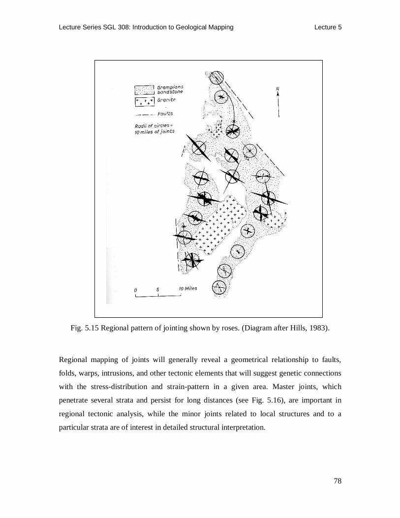
Fig. 5.15 Regional pattern of jointing shown by roses. (Diagram after Hills, 1983).
Regional mapping of joints will generally reveal a geometrical relationship to faults,
folds, warps, intrusions, and other tectonic elements that will suggest genetic connections
with the stress-distribution and strain-pattern in a given area. Master joints, which
penetrate several strata and persist for long distances (see Fig. 5.16), are important in
regional tectonic analysis, while the minor joints related to local structures and to a
particular strata are of interest in detailed structural interpretation.

Lecture Series SGL 308: Introduction to Geological Mapping Lecture 5
79
Fig. 5.16 Aerial photograph of joint set in Sandstone, Wonderland Range, Australia. (Inset - Note the majorly NE-SW trend of the master joints and the minor NW-SE trends exemplified by the rose diagram). Diagram after Hills, 1983. 5.6.1.2 Faults
Similar roses may be drawn for faults representing their direction of dip, where the
exposures may mainly be in road or railway cuttings. The fault diagram shown in Fig.
5.17 demonstrates the predominance of fault dips in the SW – NW sector.
Fig. 5.17 Fault Dip roses in strongly folded Silurian rocks.
5.6.1.3 Palaeocurrent Analysis
The following cross-bedding foreset azimuths have been measured within the Baraka
sandstone outcrops in a Gondwana coal basin. Work out the mean Palaeocurrent
direction.

Lecture Series SGL 308: Introduction to Geological Mapping Lecture 5
80
The directions measured are: 5o, 25o, 45o, 48o, 50o, 315o, 322o, 330o, 332o, 335o, 336o,
337o, 338o, 342o, 352o.
Solution:
A statistical number of observations (i.e. frequency) of the data sets are presented in
Table 5.2.
Table 5.2: Directional data of Baraka sandstone.
Interval Midpoint No. of observations
0o-19o
20o – 39o
40o – 59o
300o – 319o
320o – 339o
340o – 359o
9.5o
29.5o
49.5o
309.5o
329.5o
349.5o
1
1
3
1
8
2
Total 16
A graphical presentation (circular histogram) of the directional data presented in Table
5.2 is shown in Figure 5.
Fig. 5.18: Circular histogram (rose diagram) of the directional data shown in Table 5.2. The arrow indicates direction of the resultant vector.( Diagram after Sengupta, 2008).
Lecture Series SGL 308: Introduction to Geological Mapping Lecture 5
81
5.7 THIN- AND POLISHED-SECTION PREPARATIONS
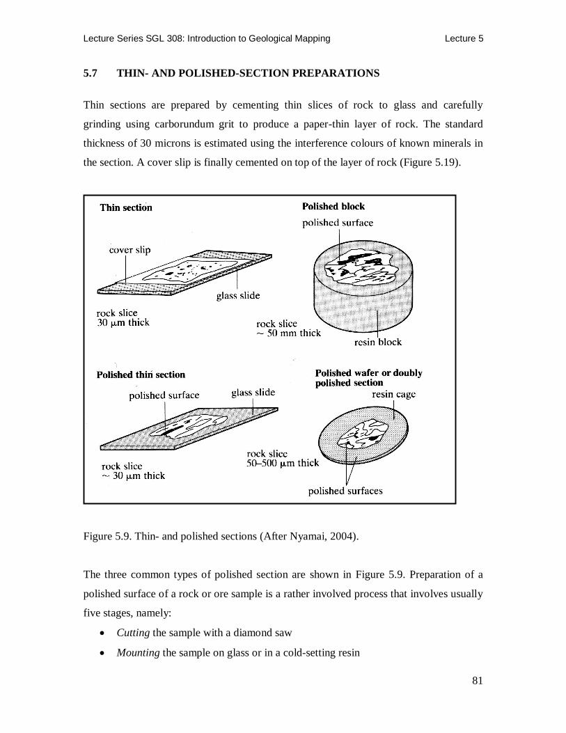
Thin sections are prepared by cementing thin slices of rock to glass and carefully
grinding using carborundum grit to produce a paper-thin layer of rock. The standard
thickness of 30 microns is estimated using the interference colours of known minerals in
the section. A cover slip is finally cemented on top of the layer of rock (Figure 5.19).
Figure 5.9. Thin- and polished sections (After Nyamai, 2004).
The three common types of polished section are shown in Figure 5.9. Preparation of a
polished surface of a rock or ore sample is a rather involved process that involves usually
five stages, namely:
Cutting the sample with a diamond saw
Mounting the sample on glass or in a cold-setting resin

Lecture Series SGL 308: Introduction to Geological Mapping Lecture 5
82
Grinding the surface flat using carborundum grit and water on a glass or a metal
surface
Polishing the surface using diamond grit and an oily lubricant on a relatively hard
“paper” lap.
Buffing the surface using gamma alumina powder and water as lubricant on a
relatively soft “cloth” lap.
5.8 Summary
In this lecture you have learned that the study of rocks involves many methods, and the
procedures followed depend on the nature of the rock, the purpose of the study, and the
facilities and time available. In particular you have learned the principle of operation of
the petrographic microscope and how to determine the form, crystallographic and optical
properties of minerals.
We learned about the principles of operation of the major X-ray and chemical methods of
rock analyses. These methods included the X-ray fluorescence (XRF), atomic absorption
spectroscopy (AAS), X-ray diffraction, electron microscopy, scanning electron
microscopy and radiography of rock slabs among others. In this lecture we also learned
how structures can be analyzed statistically using spherical projections with the ultimate
There are many variants of the procedure described for thin- and
polished section preparation, and the details usually depend on the
nature of the samples and the polishing materials, and equipment that
happen to be available. Whatever the method used, the objective is a
flat, relief-free, scratch-free polished surface.

Lecture Series SGL 308: Introduction to Geological Mapping Lecture 5
83
purpose of understanding their characteristic deformational movements. Finally we
learned how thin sections are prepared by cementing thin slices of rock to glass and
carefully grinding using carborundum grit to produce a paper-thin layer of rock.
5.9 References
Berry, LG., Mason, B. and Dietrich, R.V. 1983. Mineralogy: Concepts, Descriptions and
Determinations. W.H. Freeman and Company, San Francisco, 561 pp.
Ehlers, E.G. and Blatt, H. (1999). Petrology: Igneous, Sedimentary and Metamorphic.
CBS Publishers & Distributors, p289.
Hills, E.S. (1983). Elements of Structural Geology. Chapman and Hall Publishers, pp
502.
Nyamai, C.M. (2004). Principles of Mineralogy Lecture Series, Nairobi University Press,
pp 125.
Sengupta, S.M. (2008). Introduction to Sedimentology. 2nd Ed. CBS Publishers &
Distributers, India.