1

Laboratory – 4

AC Circuits Phasors, Impedance and Transformers

Objectives The objectives of this laboratory are to gain practical understanding of circuits in the sinusoidal steady state and experience with

• series RC, RL and RLC circuits, • calculating and measuring impedance, • measuring and graphing phasors and phase shift between voltage and current, • observing impedance change as a function of changing the frequency of the applied

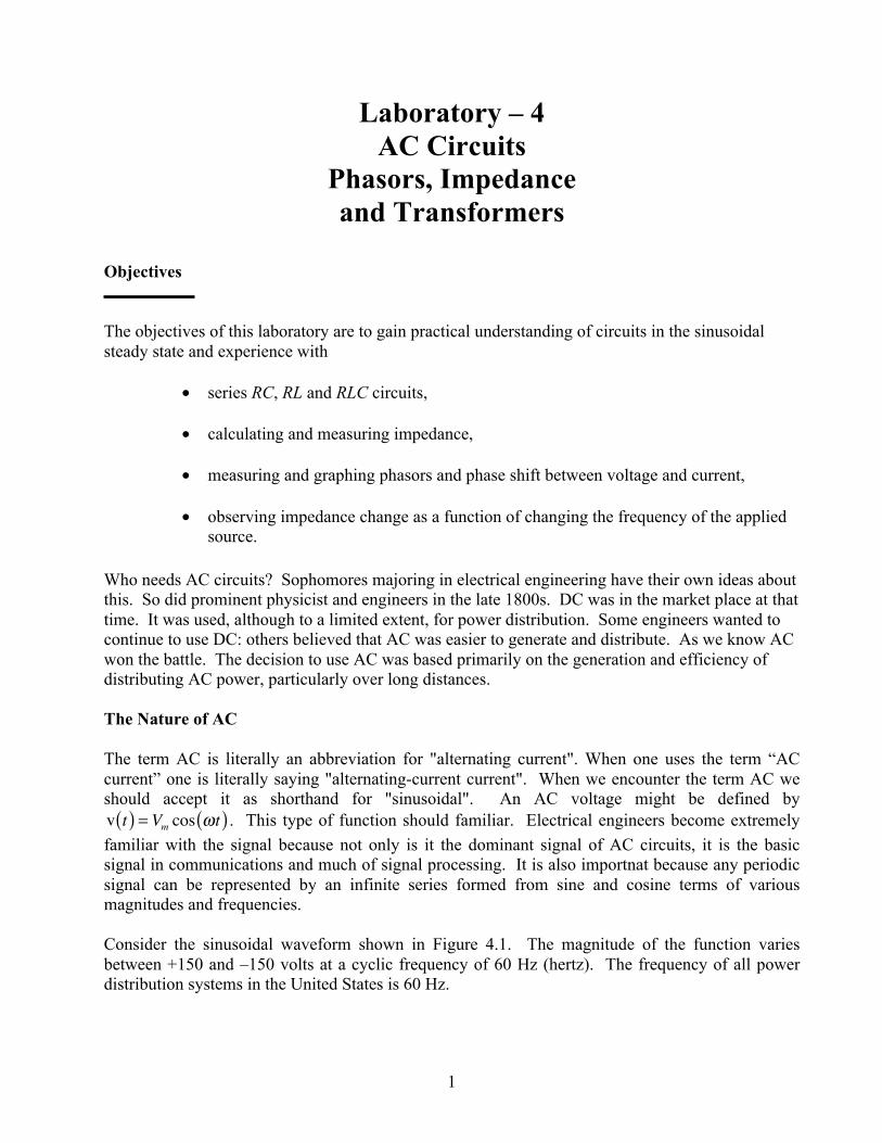
source. Who needs AC circuits? Sophomores majoring in electrical engineering have their own ideas about this. So did prominent physicist and engineers in the late 1800s. DC was in the market place at that time. It was used, although to a limited extent, for power distribution. Some engineers wanted to continue to use DC: others believed that AC was easier to generate and distribute. As we know AC won the battle. The decision to use AC was based primarily on the generation and efficiency of distributing AC power, particularly over long distances. The Nature of AC The term AC is literally an abbreviation for "alternating current". When one uses the term “AC current” one is literally saying "alternating-current current". When we encounter the term AC we should accept it as shorthand for "sinusoidal". An AC voltage might be defined by v t( ) = Vm cos ωt( ) . This type of function should familiar. Electrical engineers become extremely familiar with the signal because not only is it the dominant signal of AC circuits, it is the basic signal in communications and much of signal processing. It is also importnat because any periodic signal can be represented by an infinite series formed from sine and cosine terms of various magnitudes and frequencies. Consider the sinusoidal waveform shown in Figure 4.1. The magnitude of the function varies between +150 and –150 volts at a cyclic frequency of 60 Hz (hertz). The frequency of all power distribution systems in the United States is 60 Hz.

2

Figure 4.1 A sinusoidal voltage waveform. We recall that t (time, in seconds), f (cyclic frequency, in hertz) and ω (radian frequency, in rad/sec)

are related by ω = 2π f and f = 1T

where T is the fundamental period. The polarity of the voltage

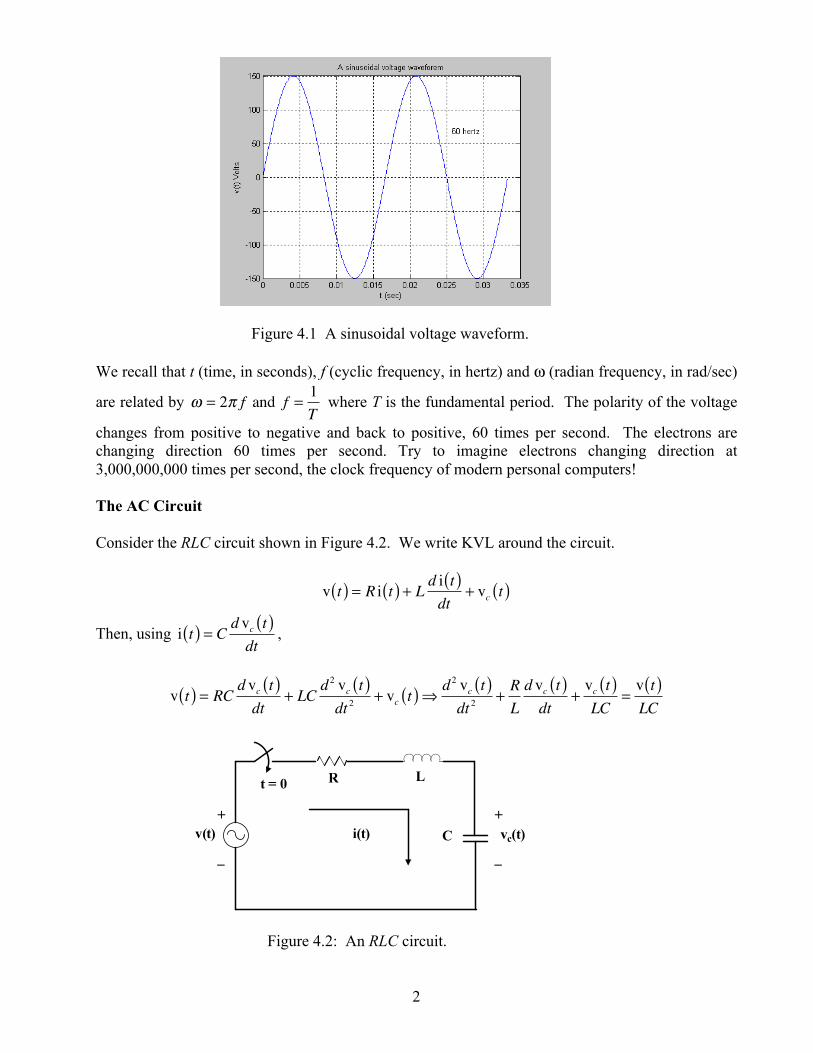
changes from positive to negative and back to positive, 60 times per second. The electrons are changing direction 60 times per second. Try to imagine electrons changing direction at 3,000,000,000 times per second, the clock frequency of modern personal computers! The AC Circuit Consider the RLC circuit shown in Figure 4.2. We write KVL around the circuit.

v t( ) = R i t( ) + L d i t( )dt

+ vc t( )

Then, using i t( ) = C d vc t( )dt

,

v t( ) = RC d vc t( )dt

+ LCd 2 vc t( )dt 2

+ vc t( )⇒ d 2 vc t( )dt 2

+RLd vc t( )dt

+vc t( )LC

=v t( )LC

Figure 4.2: An RLC circuit.

3

This is a linear, constant-coefficient, second-order, inhomogeneous, ordinary differential equation. We have seen this equation in our study of transients. Although methods of solving this equation are well known, that does not make it a simple problem, especially if the characteristic equation has complex roots. A typical waveform of the capacitor voltage for a 60 Hz input signal is shown in Figure 4.3. The transient dies quickly. After the transient dies away all that is left is the steady-state solution which is easier to find.

Figure 4.3 Typical response of a RLC circuit with a sinusoidal input. If we apply a sinusoidal signal as the forcing function of the differential equation, the steady state solution will also be a sinusoidal of the form

vc t( ) = K cos ωt +θ( ) We only need to solve for K and θ to have the steady state solution. A German-Austrian mathematician and engineer, C. P. Steinmetz, 1865-1923, who migrated to America and worked for General Electric (he liked to smoke cigars on the shop floor at GE!), introduced the concept of solving for K and θ by using phasors. The detailed background for phasors is found in any basic circuits text. We only consider the essentials here. To solve an AC circuit for a steady state voltage or current we use the following: A voltage of the form Vm cos ωt +θ( ) is replaced by its phasor equivalent Vm∠θ . For circuit elements; R is unchanged, L is replaced by jωL and C is replaced by 1 / jωC For AC circuit analysis, Figure 4.2 becomes

4

Figure 4.4 Circuit for AC steady state analysis. As an example, let the input voltage be 100cos(2π60t + 30o). Let

R = 100Ω , L = 0.25H , C = 10µF We note that ω = 2π60 = 377. This is used in finding jωL and 1 / jωC . The circuit of Figure 4.4, with values added, is shown in Figure 4.5.

Figure 4.5 Series AC circuit. The solution for the phasor current I is

I = 100∠30°100 + j94 − j265

= 0.51∠90° A

The actual time variation of current is then i t( ) = 0.51cos 377t + 90°( ) A The phasor capacitor voltage is (using voltage division adapted to AC circuits)

VC =− j265

100 + j94 − j265100∠30° = 133.8∠− 0.3°

Vc contains all the information we need to write vC t( ) = 133.8cos 377t − 0.3°( ) V . In many cases we don't bother to write the time domain solution of AC voltages and currents. Phasors give us all the information we need for practically all AC circuit analysis.

5

The Impedance Concept Impedance is a concept arising from the method of undetermined coefficients used in finding the steady state solution of a differential equation. Fortunately, all the rules we learned about resistance in DC circuits carry over to impedance in AC circuits. Impedance, in general, is a complex number composed of a real part and an imaginary part. We write impedance as Z = R + jX . Z has units of ohms. X (called reactance) can be either positive or negative. Consider the circuit below that is expressed with Z’s.

Figure 4.6 Finding impedance of an AC circuit.

ZEQ = Z1 +Z2 Z3 + Z4( )Z2 + Z3 + Z4

Impedance is calculated just as we calculated resistance, through series and parallel combinations. There are two major differences between resistance and impedance. First, impedance has a both a real part and an imaginary part. Resistance has only a real part (Its imaginary part is zero). Second, resistance does not change as the frequency of the applied voltage changes. The value of impedance does change as a function of the frequency of the applied voltage. This fact has a strong effect on how circuits perform. Basic AC Circuit Properties Two of the most basic properties of DC circuits were the current division rule and the voltage division rule. These properties carry over to AC circuits with modifications to accommodate impedance and phasors. This is illustrated in the following example. We desire to find the phasor current I shown in the circuit Figure 4.7. First determine the impedance seen by the source.

6

Figure 4.7: AC circuit for example problem.

Z = 50 − j30 +j20( ) 80( )j20 + 80

= 55.8∠−11.6°

Therefore, the phasor current I is I = 100∠0°55.8∠−11.6°

= 1.79∠11.6° . If we want to find the currents

IA and IB we can use current division, in the same way we do for resistive circuits.

IA =80

j20 + 801.79∠11.6° = 1.737∠− 2.44°

IB =j20

j20 + 801.79∠11.6° = 0.434∠87.6°

If we want to find voltages VA and VB we can use voltage division in the same format as used for DC circuits.

VA =50 − j30

50 − j30 + 80 j20( )80 + j20

100∠0° = 104.4∠−19.4°

and

VB =

80 j20( )80 + j20

50 − j30 + 80 j20( )80 + j20

100∠0° = 34.8∠87.6°

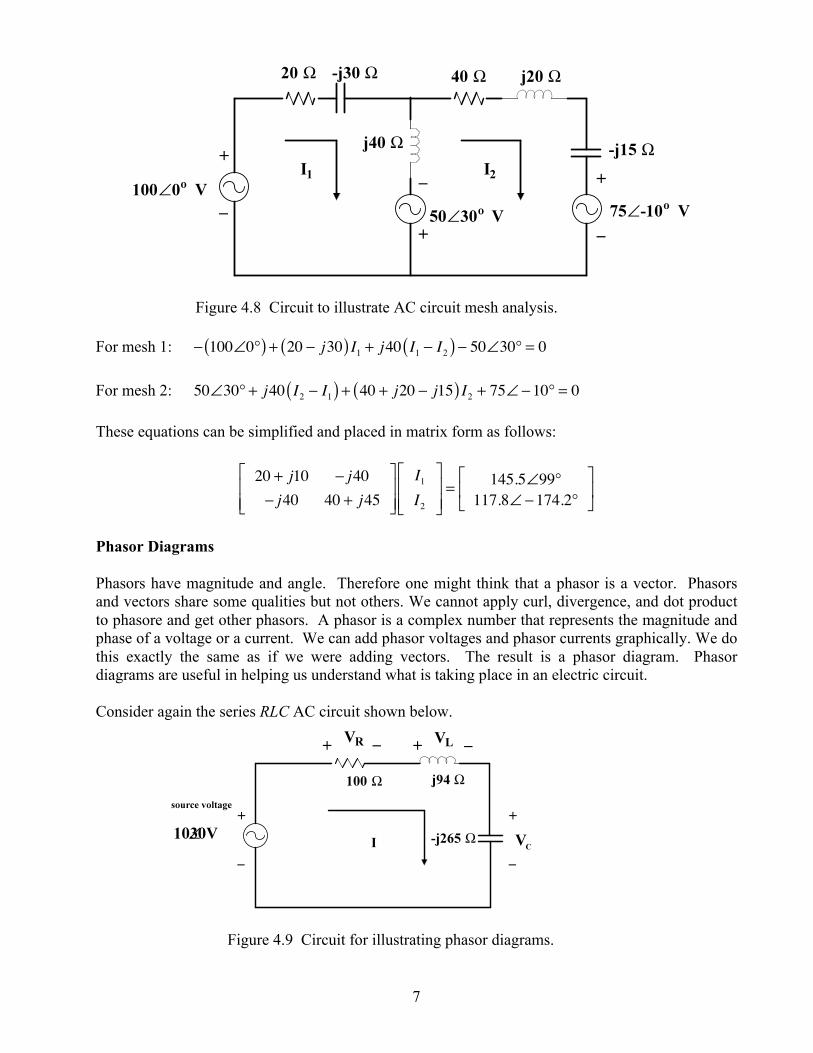
We can also apply mesh analysis and nodal analysis to AC circuits much in the same manner that we did for DC circuits. We illustrate this with a mesh analysis problem. Consider the circuit shown in Figure 4.8.

7

Figure 4.8 Circuit to illustrate AC circuit mesh analysis. For mesh 1: − 100∠0°( ) + 20 − j30( ) I1 + j40 I1 − I2( ) − 50∠30° = 0 For mesh 2: 50∠30° + j40 I2 − I1( ) + 40 + j20 − j15( ) I2 + 75∠−10° = 0 These equations can be simplified and placed in matrix form as follows:

20 + j10 − j40− j40 40 + j45

⎡

⎣⎢⎢

⎤

⎦⎥⎥

I1I2

⎡

⎣⎢⎢

⎤

⎦⎥⎥= 145.5∠99°

117.8∠−174.2°⎡

⎣⎢

⎤

⎦⎥

Phasor Diagrams Phasors have magnitude and angle. Therefore one might think that a phasor is a vector. Phasors and vectors share some qualities but not others. We cannot apply curl, divergence, and dot product to phasore and get other phasors. A phasor is a complex number that represents the magnitude and phase of a voltage or a current. We can add phasor voltages and phasor currents graphically. We do this exactly the same as if we were adding vectors. The result is a phasor diagram. Phasor diagrams are useful in helping us understand what is taking place in an electric circuit. Consider again the series RLC AC circuit shown below.

Figure 4.9 Circuit for illustrating phasor diagrams.

8

We saw earlier that the phasor current was I = 0.51∠90° A . We can use this value to calculate the three phasor voltages VR , VL and VC shown in Figure 4.9.

VR = 0.51∠90° ×100 = 51∠90° V

VL = 0.51∠90° × j94 = 47.9∠180° V

VC = 0.51∠90° × − j265( ) = 135∠0° V Within calculator round-off accuracy we will find that V = VR +VL +VC as it should, according to KVL. A phasor diagram showing the above four voltages is given in Figure 4.10 You will be making a phasor diagram from your laboratory measurements.

Figure 4.10 Phasor diagram for the AC circuit of Figure 4.9. Transformers Three major areas in which we use transformers are in (a) power distribution, (b) converting AC voltage to DC voltage, and (c) electronics.

9

Of these three, the power transformers used for stepping-up and stepping-down voltage are the most familiar and the most widely used application of this device. Power transformers can be very large. Most of us have seen the giant transformers in substation yards. These require using special cooling fans and a circulating fluid. At the next level we find transformers used in distributing power to industry and residential areas. We have all seen transformers mounted on power poles and in more modern subdivisions, mounted in a metal housing at ground level. You will have the opportunity to study more about power transformers in your junior year. For this laboratory exercise we will focus on the transformers used in electronics. In electronics, small transformers (compared to power transformers) are frequently used for converting AC to DC. In addition to AC to DC conversion, transformers are also used for isolating one circuit from another and for impedance matching. In this laboratory exercise you will take a brief look at the application of stepping-up and stepping-down voltage (current) and impedance reflection from one side of the transformer to the other. One can separate transformers into two categories: the linear transformers and the ideal transformer. The coils of a linear transformer are wound on a non-magnetic material such as plastic, wood, and air core. Refer to your text for a further explanation of how to analyze the linear transformer. A brief background of the ideal transformer is given in the following paragraphs. Three main distinguishing features of the ideal transformer are

• The inductances L1, L2 and M are very large ideally infinite. In this case L1 is the inductance on the primary side of the transformer, L2 the inductance on the secondary side and M the mutual inductance.

• The coefficient of coupling of the transformer is unity. This implies that the coils

are tightly wound with respect to one another. In reality they are wound together, with the wires of the primary intermeshed with those of the secondary.

• The coils are lossless. That is, the resistances ( R1 and R2 ) of both the primary and

secondary are ideally zero.

The schematic (symbol) used for the ideal transformer is shown in Figure 4.11.

Figure 4.11 Schematic of the ideal transformer.

10

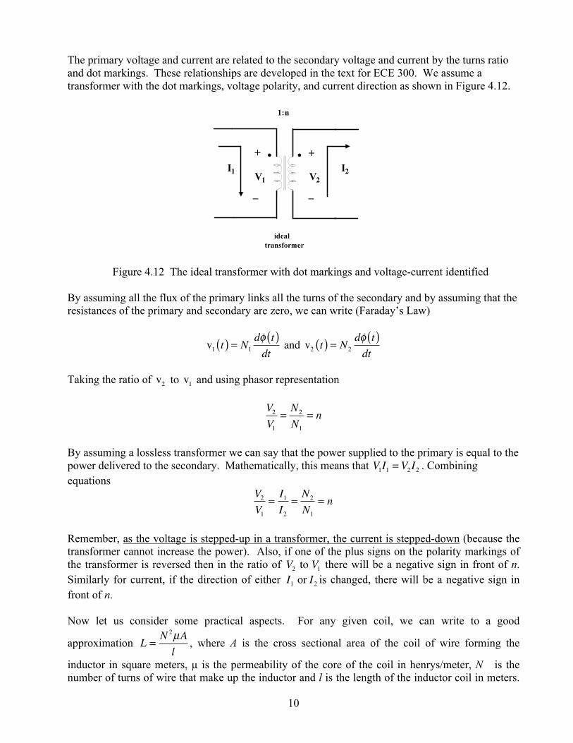
The primary voltage and current are related to the secondary voltage and current by the turns ratio and dot markings. These relationships are developed in the text for ECE 300. We assume a transformer with the dot markings, voltage polarity, and current direction as shown in Figure 4.12.

Figure 4.12 The ideal transformer with dot markings and voltage-current identified By assuming all the flux of the primary links all the turns of the secondary and by assuming that the resistances of the primary and secondary are zero, we can write (Faraday’s Law)

v1 t( ) = N1dφ t( )dt

and v2 t( ) = N2dφ t( )dt

Taking the ratio of v2 to v1 and using phasor representation

V2V1

=N2

N1= n

By assuming a lossless transformer we can say that the power supplied to the primary is equal to the power delivered to the secondary. Mathematically, this means that V1I1 = V2I2 . Combining equations

V2V1

=I1I2

=N2

N1= n

Remember, as the voltage is stepped-up in a transformer, the current is stepped-down (because the transformer cannot increase the power). Also, if one of the plus signs on the polarity markings of the transformer is reversed then in the ratio of V2 to V1 there will be a negative sign in front of n. Similarly for current, if the direction of either I1 or I2 is changed, there will be a negative sign in front of n. Now let us consider some practical aspects. For any given coil, we can write to a good

approximation L =N 2µAl

, where A is the cross sectional area of the coil of wire forming the

inductor in square meters, µ is the permeability of the core of the coil in henrys/meter, N is the number of turns of wire that make up the inductor and l is the length of the inductor coil in meters.

11

To make L large, in particular to make it approach infinity as stated in the assumption of the ideal transformer, requires many turns, a large cross sectional area, small l and high permeability. Various combinations of these can be used to increase L. For example, the relative permeability of iron and steel are approximately 5000 times greater than air. The ideal transformer uses a ferromagnetic material such as laminated steel alloy to increase L. Invariably, for audio transformers, the number of turns N is made large to increase L. In making N large, one usually uses a small gauge wire to control the physical size and weight of the transformer. We recall that

the resistance of wire is given by R =ρLA

where A is the cross section area of the wire in square

meters, l is the length of the wire in meters and ρ is resistivity (usually of copper) in ohm ⋅meters . Using small gauge wire and lots of turns for making the coil leads to high resistance in the coil of the inductor. As a reference point, the small transformer included in the ECE 300 parts kit has a nominal primary inductance of 19.2 H, along with a resistance of 200 ohms. Each secondary has about 0.45 H with 15 ohms. In this case the primary has about 4.4 times the number of turns of the secondary. As another example, the small inductor used in this lab for the AC circuits work has 100 mH and a nominal resistance of 90 ohms. Before considering a realistic model of the ideal transformer in application, first we consider the ideal case as shown in Figure 4.13.

Figure 4.13 Ideal transformer configuration. It is easy to show that the load impedance is reflected as shown in Figure 4.14 for the this case.

Figure 4.14 Reflected load resistance for a ideal transformer. A more realistic model of an ideal transformer (accounting for the resistance of the windings) that has a source voltage along with a series resistor and a load resistance would be as shown below.

12

Figure 4.15 Ideal transformer including coil resistance. A circuit showing how the resistance is reflected to the source side of the transformer is shown in Figure 4.16. We have found that this model gives reasonable results when using the transformer of the ECE 300 kit. You will be measuring the source side voltage Vss in the laboratory.

Figure 4.16 Diagram showing load resistance reflected to source in modified ideal transformer circuit. The reason the transformer is used in this manner is that often, particularly in electronics, a speaker will be connected to a power amplifier. We would like to have maximum power transfer. We recall that the load resistance and the source resistance should be the same for achieving maximum power transfer. For example, if the power amplifier had 1000 ohms output resistance and one had a transformer with n = 10, then ideally a 10 ohm load resistor would be reflected as 1000 ohms and maximum power transfer would be achieved. Prelab Exercises Complete the following exercises prior to coming to the lab. As usual, turn-in your prelab work to the lab instructor before starting the Laboratory Exercises. Part I PE: Half wave rectifier. The purpose of this exercise is to illustrate the nature of the positive polarity and negative polarity of a sinusoidal signal. Assume you are given a 4700 Ω resistor and a 1N4004 diode. You are to use these elements in a circuit connected to a sinusoidal signal source so that you produce the signals shown in Figure 4.17. Show your circuit diagram that produces these waveforms.

13

(a) voltage on positive swing of sine wave (b) voltage on negative swing of sine wave

Figure 4.17 Desired voltage waveforms, Part 1PE. Part 2 PE: Circuit impedance. Consider the circuit of Figure 4.18.

Figure 4.18 Circuit for determining impedance, Part 2PE. If this circuit has a 1000 Hz source connected between terminals a and b, determine Zin. Part 3PE: Series RC circuit. Consider the circuit shown in Figure 4.19.

14

Figure 4.19 AC circuit for Part 3PE.

(a) Calculate the phasor voltages VR and VC .

(b) Draw the phasor diagram showing Vsource , VR and VC . Part 4PE: Series RLC circuit. Consider the circuit of Figure 4.20.

Figure 4.20 AC circuit for Part 4PE.

(a) In the following calculations, ignore the 90 Ω resistance that is inherent with the transformer coil. Calculate the phasor voltages VR , VL and VC when the frequency of the input signal is 1000 Hz.

(a) Draw the phasor diagram showing Vsource , VR , VC and VL .

Part 5PE:

(a) Consider the circuit shown in Figure 4.21. Calculate the total resistance the source will see, to the right of P1-P2, after the 20 Ω load resistance and the 15 Ω resistance in the S1-S2 coil are reflected to the source side of the transformer and the 200 ohms present from the source side of the transformer is added to the reflected resistance.

15

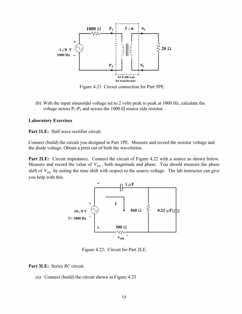
Figure 4.21 Circuit connection for Part 5PE.

(b) With the input sinusoidal voltage set to 2 volts peak to peak at 1000 Hz, calculate the voltage across P1-P2 and across the 1000 Ω source side resistor.

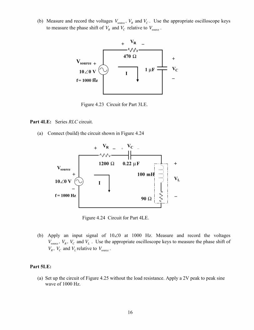
Laboratory Exercises Part 1LE: Half wave rectifier circuit. Connect (build) the circuit you designed in Part 1PE. Measure and record the resistor voltage and the diode voltage. Obtain a print out of both the waveforms. Part 2LE: Circuit impedance. Connect the circuit of Figure 4.22 with a source as shown below. Measure and record the value of V300 , both magnitude and phase. You should measure the phase shift of V300 by noting the time shift with respect to the source voltage. The lab instructor can give you help with this.

Figure 4.22: Circuit for Part 2LE. Part 3LE: Series RC circuit.

(a) Connect (build) the circuit shown in Figure 4.23

16

(b) Measure and record the voltages Vsource , VR and VC . Use the appropriate oscilloscope keys to measure the phase shift of VR and VC relative to Vsource .

Figure 4.23 Circuit for Part 3LE. Part 4LE: Series RLC circuit.

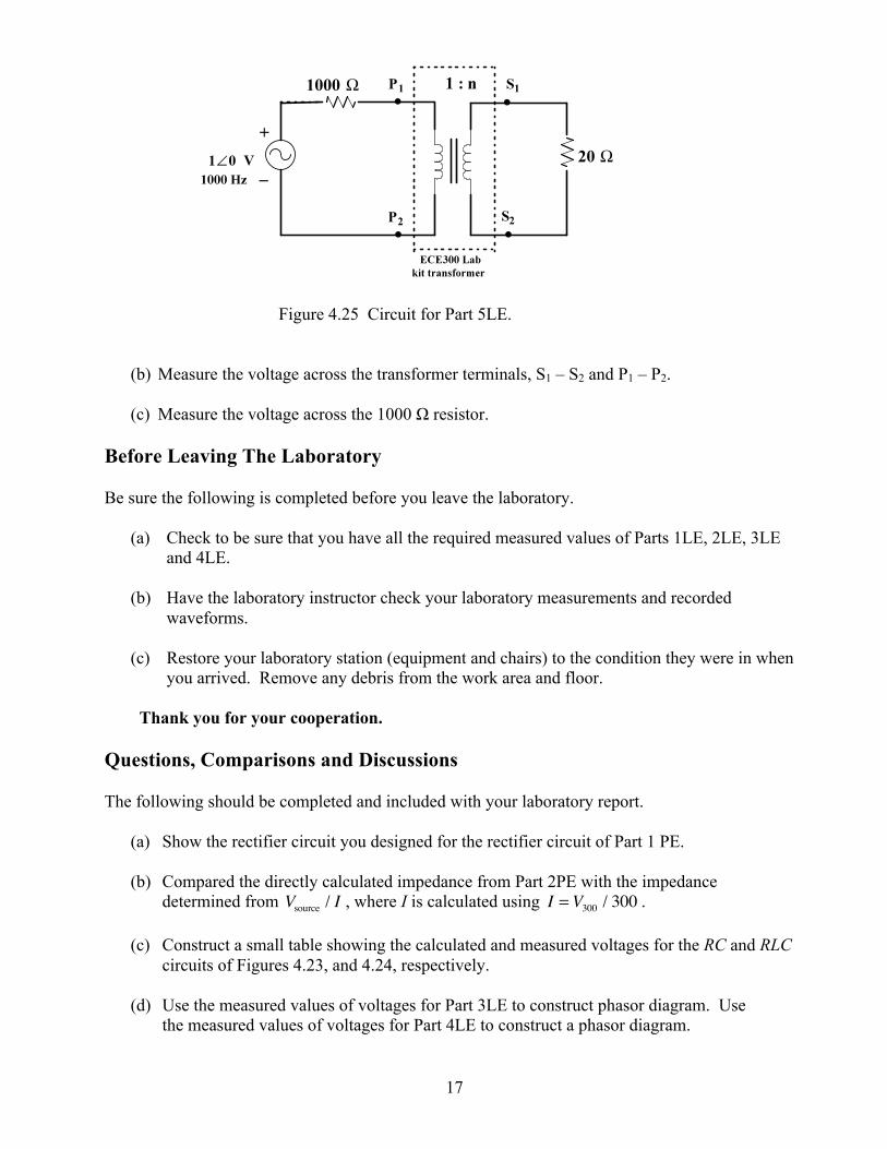
(a) Connect (build) the circuit shown in Figure 4.24

Figure 4.24 Circuit for Part 4LE.

(b) Apply an input signal of 10∠0 at 1000 Hz. Measure and record the voltages Vsource , VR , VC and VL . Use the appropriate oscilloscope keys to measure the phase shift of VR , VC and VL relative to Vsource .

Part 5LE:

(a) Set up the circuit of Figure 4.25 without the load resistance. Apply a 2V peak to peak sine wave of 1000 Hz.

17

Figure 4.25 Circuit for Part 5LE. (b) Measure the voltage across the transformer terminals, S1 – S2 and P1 – P2. (c) Measure the voltage across the 1000 Ω resistor.

Before Leaving The Laboratory Be sure the following is completed before you leave the laboratory.

(a) Check to be sure that you have all the required measured values of Parts 1LE, 2LE, 3LE and 4LE.

(b) Have the laboratory instructor check your laboratory measurements and recorded

waveforms.

(c) Restore your laboratory station (equipment and chairs) to the condition they were in when you arrived. Remove any debris from the work area and floor.

Thank you for your cooperation. Questions, Comparisons and Discussions The following should be completed and included with your laboratory report.

(a) Show the rectifier circuit you designed for the rectifier circuit of Part 1 PE.

(b) Compared the directly calculated impedance from Part 2PE with the impedance determined from Vsource / I , where I is calculated using I = V300 / 300 .

(c) Construct a small table showing the calculated and measured voltages for the RC and RLC

circuits of Figures 4.23, and 4.24, respectively.

(d) Use the measured values of voltages for Part 3LE to construct phasor diagram. Use the measured values of voltages for Part 4LE to construct a phasor diagram.

18

Laboratory Report The following should be included in your laboratory report. If you have any questions be sure to contact the lab instructor.

(a) Give a short summary (50 to 100 words) of what is to be accomplished in the lab exercise. (b) Write the procedure followed for each part of lab Work.

(c) Tabulate all you readings.

(d) Present all the printouts of the oscilloscope screen neatly labeled. (e) Answer the questions listed above. (f) Write a brief conclusion (approximately 200 words)

(g) Attach the graded prelab at the end of your report.