Labor supply distortions ofpension fund recovery policies∗

Roel Mehlkopf†

April 21, 2009

Abstract

This paper studies the distortions in labor supply choices that are induced by the recoverypolicies of pension funds. Pension funds recover from funding shortfalls and surpluses by makingadjustments in the contribution rate charged to participants and/or adjusting the value of pensionaccruals received by participants in return. Deviations between contribution and accrual ratesimply that the pension fund levies a net tax or provides a net subsidy on the labor supply of itsparticipants. The resulting distortions in labor supply choices cause labor earnings to become morepositively correlated to stock returns, thereby reducing the risk-bearing capacity of participants.Recovery policies prevent pension funds from taking optimal advantage of the risk premium infinancial markets. Labor supply distortions are eliminated if financial gains and losses are leviedupon participants through lump-sum transfers, rather than through transfers that are proportionalto labor supply. My analysis suggests that this policy improvement results in an ex ante welfaregain of almost a full percentage point in terms of certainty equivalent consumption.

Keywords: Saving, investment, labor supply, life cycle, pension funds.JEL classification: D91, G11, G23, H23

∗The author thanks Frank de Jong and Lans Bovenberg for their help and encouragement.†Tilburg University, CentER and Netspar. Email: R.J.Mehlkopf@TilburgUniversity.nl.

1 Introduction

Bodie, Merton, and Samuelson (1992) have shown that the labor-leisure choice plays an

important role in intertemporal saving and investment decision making over the life cycle.

They describe that income effects in labor supply provide a buffer against wealth shocks,

causing labor supply flexibility to be a pure blessing in their analysis. A negative wealth

shock causes the marginal utility from working to increase, whereas a positive wealth shock

has an opposite effect. The resulting pro-cyclical labor supply behavior causes labor earnings

to become more negatively correlated to stock returns, increasing the individual’s appetite

for risk taking. In the analysis of Bodie, Merton, and Samuelson (1992) an increase in labor

supply flexibility therefore enables individuals to benefit more from the risk premium in

financial markets, resulting in an increase in ex ante welfare levels.

In this paper I study the shadow side of labor supply flexibility for individuals that are

saving for retirement in a collective pension fund. Pension funds apply recovery policies by

which financial gains and losses are levied upon the future earnings of participants through

adjustments in contribution and accrual rates. Given that the effective wage rate of a pension

fund participant is equal to the wage rate minus the contribution rate plus the accrual rate,

deviations between contribution and accrual rates induce a wage differential. Pension funds

thus recover from financial shocks by levying a net tax or providing a net subsidy upon

the labor earnings of participants, thereby introducing substitution effects in labor supply

decisions. These substitution effects in labor supply have exactly the opposite implications

as the income effects in labor supply analyzed by Bodie, Merton, and Samuelson (1992).

Recovery policies induce pro-cyclical labor supply behavior because labor supply is taxed in

bad economic times (during which the funding status needs to recover from financial losses)

and subsidized in good times. Pro-cyclical labor supply behavior causes the labor earnings of

participants to become more positively correlated to stock returns, reducing the risk bearing

capacity of pension fund participants. The recovery policies of pension funds thus prevent

participants from taking full advantage of the risk premium in financial markets, resulting

in a decline in ex ante welfare levels.

My analysis recognizes that recovery policies also have a welfare improving effect for a

1

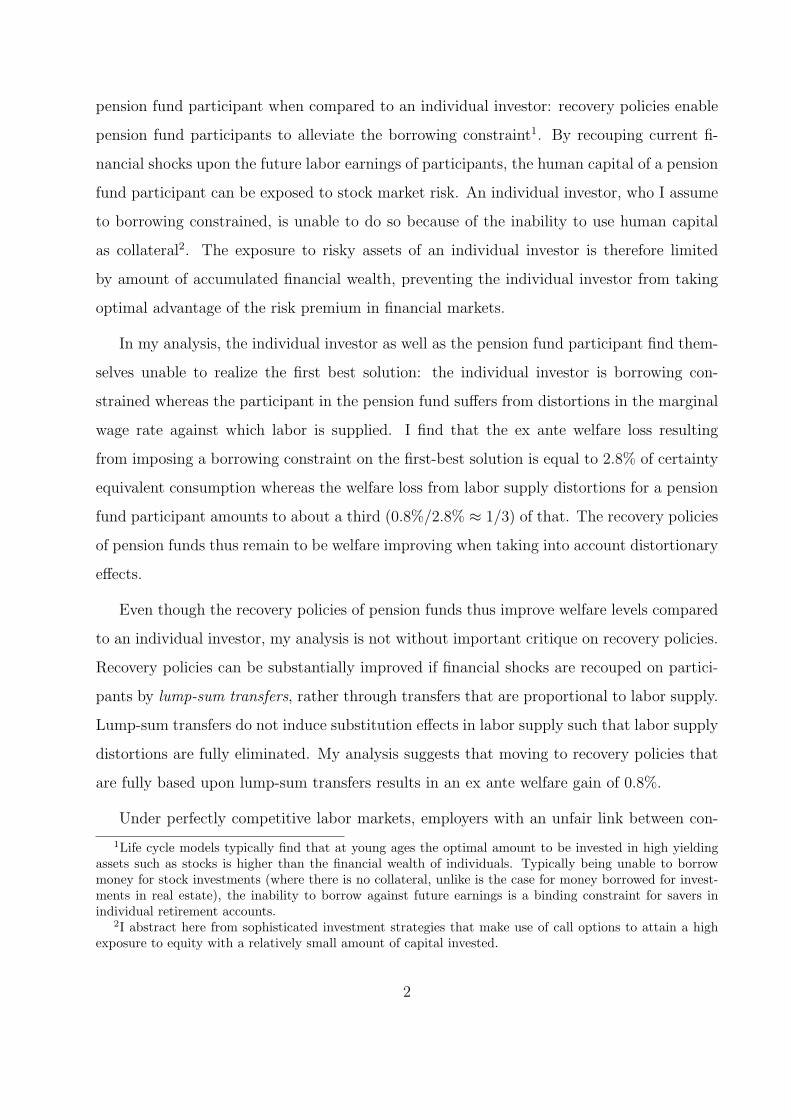
pension fund participant when compared to an individual investor: recovery policies enable

pension fund participants to alleviate the borrowing constraint1. By recouping current fi-

nancial shocks upon the future labor earnings of participants, the human capital of a pension

fund participant can be exposed to stock market risk. An individual investor, who I assume

to borrowing constrained, is unable to do so because of the inability to use human capital

as collateral2. The exposure to risky assets of an individual investor is therefore limited

by amount of accumulated financial wealth, preventing the individual investor from taking

optimal advantage of the risk premium in financial markets.

In my analysis, the individual investor as well as the pension fund participant find them-

selves unable to realize the first best solution: the individual investor is borrowing con-

strained whereas the participant in the pension fund suffers from distortions in the marginal

wage rate against which labor is supplied. I find that the ex ante welfare loss resulting

from imposing a borrowing constraint on the first-best solution is equal to 2.8% of certainty

equivalent consumption whereas the welfare loss from labor supply distortions for a pension

fund participant amounts to about a third (0.8%/2.8% ≈ 1/3) of that. The recovery policies

of pension funds thus remain to be welfare improving when taking into account distortionary

effects.

Even though the recovery policies of pension funds thus improve welfare levels compared

to an individual investor, my analysis is not without important critique on recovery policies.

Recovery policies can be substantially improved if financial shocks are recouped on partici-

pants by lump-sum transfers, rather through transfers that are proportional to labor supply.

Lump-sum transfers do not induce substitution effects in labor supply such that labor supply

distortions are fully eliminated. My analysis suggests that moving to recovery policies that

are fully based upon lump-sum transfers results in an ex ante welfare gain of 0.8%.

Under perfectly competitive labor markets, employers with an unfair link between con-

1Life cycle models typically find that at young ages the optimal amount to be invested in high yieldingassets such as stocks is higher than the financial wealth of individuals. Typically being unable to borrowmoney for stock investments (where there is no collateral, unlike is the case for money borrowed for invest-ments in real estate), the inability to borrow against future earnings is a binding constraint for savers inindividual retirement accounts.

2I abstract here from sophisticated investment strategies that make use of call options to attain a highexposure to equity with a relatively small amount of capital invested.

2

tribution and accrual rates find themselves forced to offer compensating wage differentials

to plan participants. After all, any difference to the market wage level induces an influx or

outflow of employees if competition is perfect. Under these conditions it is thus the employer

who fully bears the funding risk of the pension plan3. However, the employer is unlikely to

(fully) bear the funding risk of the pension plan for two reasons. First, the workings of actual

labor markets are a far cry from perfectly competitive labor markets, due to the costs of

switching employers, the accumulation of company-specific human capital and the fact that

pay schemes are often based upon seniority instead of productivity. Additionally, alternative

employers may have the same pension fund (pension funds can cover a complete sector or

industry) or a pension fund with a similar funding status. For all these reasons, workers are

likely to bear a part of the wage differential themselves. For simplicity, I abstract fully from

compensating wage differentials provided by the employer.

The complexity of my analysis is dramatically reduced by the fact that income effects

in labor supply decisions are ignored. The motivation for this model simplification is that

I am not so much interested in absolute labor supply levels but merely in the difference

between in the labor supply choices of the pension fund participant and those in the first-

best strategy. The income effects in labor supply of the pension fund participant are very

similar to those in the first-best strategy, such that income effects in labor supply are of

second order importance. My analysis therefore solely focuses on substitution effects in

labor supply decisions4.

For wage differentials to affect labor supply decisions, the wage-elasticity of labor supply

should be positive. There is overwhelming evidence in the empirical labor supply literature5

3Rauh (2006) shows that such risk sharing by the employer leads to a reduction in the profitability of theplan sponsor through inefficient decision making on capital expenditures.

4Given that income effects in labor supply have a stabilizing effect on wealth, the absence of incomeeffects causes the model to overestimate the volatility in labor earnings, resulting in welfare costs of laborsupply distortions that are too high. This effect may be regarded as being offset by the fact that I assumethe wage rate of the participant offered by the employer to be constant over time during the working period,thereby clearly underestimating the volatility in labor earnings.

5Findings on labor supply elasticities are often obtained from empirical studies on the impact of a changein marginal rate of payroll taxes on the labor supply decisions of workers. Such estimates for labor supplyelasticities can be used as parameters for the labor supply responses with respect to changes in contributionrates, since they directly affect disposable income levels. However, one could question whether these pa-rameters are also useful when studying the effects of changes in accrual rates. The literature on behavioraleconomics has found convincing evidence that individuals suffer from hyperbolic discounting, suggesting that

3

that this indeed is the case. Recent overviews of Blundell and MaCurdy (1999) and Alesina,

Gleaser, and Sacerdote (2005) find a consensus in the empirical labor supply literature that

the compensated labor supply elasticity of male workers is low and that 0.2 is a reasonable

estimate, whereas the median estimate found for the labor supply of women is about 1.0.

Due to the large variation in the estimates found for females, a conservative parameter model

parameter of about 0.5 is often applied. In this paper I will work with a labor supply elasticity

of 1.0 as the default parameter. This appears to be a high estimate at first sight, but I have

two reasons to work with such a high estimate. First, labor supply distortions induced by

pension fund are likely to have a higher impact on the labor supply behavior of individuals

than distortions induced by taxes, since it may be easy for workers to evade recovery policies

by moving to self-employment or moving to an employer with an actuarially fair retirement

savings scheme. Second, my model takes the perspective of a pension fund participant who

participates in the labor force continuously until retirement, thereby abstracting from a

participation decision of workers. This ignores micro-econometric evidence that the labor

market participation of individuals responds to financial rewards (Heckman (2003), Saez

(2002)). Although less often estimated, the elasticities of labor market participation are

substantially higher than those of the number of hours worked. Eissa and Liebman (1996)

find a participation elasticity of 0.6, while Meyer and Rosenbaum (2001) find an elasticity

of 0.7.

This paper contributes to the theory on saving and investing over the life cycle. Most prior

work in this field builds on the seminal contributions of Merton (1969) and Samuelson (1969)

and treat labor earnings as exogenous (Viceira (2001), Cocco, Gomes, and Maenhout (2005),

Gomes and Michaelides (2007)). The analysis of Bodie, Merton, and Samuelson (1992)

provides the insight that income effects in labor supply increase the risk bearing capacity of

individuals and recent contributions have built on their analysis. Farhi and Panageas (2007)

and Choi, Shim, and Shin (2008) treat the case where labor supply flexibility is restricted to

choice of an irreversible and indivisible retirement date. Cvitanic, Goukasian, and Zapatero

the utility value attributed to pension accruals may be substantially lower compared to the correspondingmarket value. This suggests that the pension fund policy induces distortions in labor supply even in thesituation where contributions are equal to the market value of pension accruals. My analysis abstracts fromsuch complications.

4

(2007) allow for more general preferences for the investor and the model of Gomes, Kotlikoff,

and Viceira (2008) features realistically calibrated non-traded labor income. My paper is

the first to show that, for a pension fund participant, labor supply flexibility also induces

effects in labor supply that reduce the investor’s appetite for risk taking and decrease ex

ante welfare levels. Labor supply flexibility is thus only full of blessings as the analysis of

Bodie, Merton, and Samuelson (1992) suggests.

This paper also contributes to the literature discussing the advantages and disadvantages

of collective pension funds in comparison to individual retirement saving schemes (Teulings

and de Vries (2006), Gollier (2007), Cui, de Jong, and Ponds (2007), Bovenberg, Nijman,

Teulings, and Koijen (2007)). The advantages of collective pension funds include lower

transaction costs, possibilities to share (non-traded) risks between overlapping and non-

overlapping generations, the alleviation of the borrowing constraint and overcoming problems

related to adverse selection and the bounded rationality of individuals. On the other hand,

collective pension funds typically fail to provide tailor-made pension arrangements, apply

suboptimal policy rules with respect to consumption smoothing over the life cycle and are

often incomplete and not transparent. This paper contributes to our knowledge on the

welfare effects of pension fund policies by pointing out that the recovery policies of pension

funds can be welfare improving, also when taking into account the related labor supply

distortions. At the same time this paper stresses the importance of improving recovery

policies. Substantial welfare gains are realized by levying financial gains and losses upon

participants through lump-sum transfers, rather than through transfers that are proportional

to labor supply.

The structure of the paper is as follows. Section 2 introduces the financial market, the

life-cycle and the preferences of the individual. Section 3 introduces the first best decision

making rules. Section 4 derives the optimal strategy for an individual investor who faces a

borrowing constraint. Section 5 derives the optimal policy for the pension fund and shows

that the pension fund model corresponds to the first-best solution if labor supply is inelastic

(ε = 0) and that it corresponds to the solution of the individual investor if labor supply is

infinitely elastic (ε = ∞). Finally, section 6 concludes.

5

2 Financial market, the life-cycle and individual pref-

erences

2.1 Financial market

The individual and the pension fund have the same investment opportunities. The financial

market consists of two assets: a riskless asset which yields an instantaneous real net rate of

return r and a risky asset whose real price P (t) follows a Brownian Motion with instantaneous

volatility σ and risk premium λ:

dP (t)

P (t)= (r + σλ)dt + σdZ(t) (2.1)

for all t and where Z(t) is a standard Wiener process for which it holds that

Z(s)− Z(t) ∼ N(0, s− t) (2.2)

for all s > t. The risk premium λ represents the expected excess return (over the riskfree

rate r) per standard deviation of the excess return and is also referred to as the Sharpe

ratio. Investments in the risky asset introduce uncertainty while at the same time increasing

expected return if the risk premium is positive.

The market value at time t of a payoff X(s) with s ≥ t is given by Et

[M(s)M(t)

X(s)], where

M(t) represents the stochastic discount factor at time t and is defined by the following

stochastic differential equation:

dM(t)

M(t)= −rdt− λdZ(t) (2.3)

Throughout this paper I assume that the real riskfree rate equals 2% (r = 0.02), the volatility

of stock returns equals 20% (σ = 0.2) and the risk premium on the stock is 20% (λ = 0.2).

As a result, the expected return of risky investments in excess of the riskfree rate equals 4%.

2.2 The life cycle

Throughout this paper I consider an individual who starts working at age t0 = 25, works for

a 40-year period until the age of R = 65 and enjoys a 20-year retirement period before dying

6

at the deterministic age of T = 85. The labor supply level h(t) of the individual at time t

during the working period is a decision variable, with h(t) ≥ 0 for all t0 ≤ t < R. No labor

is supplied in the retirement period, i.e. h(t) = 0 for all R ≤ t ≤ T . The real wage level

per unit of labor supply at age t is deterministic and is denoted by w(t). The wage level is

inelastic with respect to labor supply levels, implying that the production function of the

economy features infinite elasticity of substitution between capital and labor.

2.3 Individual preferences

Preferences of the individual are given by time-separable expected utility from consumption

C(t) and labor supply h(t):

U(t) = Et

[∫ T

t

e−β(s−t)u(C(s), h(s))ds

](2.4)

for t0 ≤ t ≤ T , where β represents the individual’s rate of time preference and where the

instantaneous utility function at age t is given by:

u(C(t), h(t)) =1

1− γ

(C(t)− ε

ε + 1h(t)

ε+1ε + η

)1−γ

(2.5)

where η represents a constant that will be defined at a later point in this section, and where

ε represents the intratemporal labor supply elasticity with respect to the wage level. Thus,

an decrease in the wage level at time t by one percent results in a decline in the labor supply

level at time t of ε percent. Originating from Greenwood, Hercowitz, and Huffman (1988),

the specification in (2.5) features the property that income effects in labor supply decision

making are eliminated from labor supply supply decision. This is rather convenient given

that, as explained in the introduction, income effects in labor supply are only of secondary

importance for the purposes of my analysis.

Due to the absence of income effects, labor supply decisions are solely driven by the

intra-temporal tradeoff between consumption and leisure6. In absence of a wage differential

labor supply decisions and fully determined by the marginal wage rate w(t):

h(t) ≡ h∗(t) = w(t)ε (2.6)

6Leisure is used here in a broad sense of the term, that is any non market (or non traded) activity suchas home production, work in the black economy or, indeed, having fun.

7

for all t0 ≤ t < R. Equation (2.6) implies that labor supply levels are constant over the life

cycle if the wage rate is constant. Negative labor supply levels are ruled out by the model

as long as marginal wage levels remain positive. Whereas the labor supply of the individual

investor are given by equation (2.6), those of the pension fund participant will be different

because an ex post wage differential is induced by the recovery policy of the pension fund.

In section 5 the welfare losses from the labor supply distortions of pension fund policies

will be derived for various choices for the elasticity of labor supply parameter ε. In order to

prevent that a change in the labor supply elasticity parameter ε affects the interpretation of

the risk aversion parameter γ, I define parameter η in the utility function in equation (2.5)

as:

η =ε

ε + 1(h∗(t))

ε+1ε =

ε

ε + 1w(t)ε+1 (2.7)

where h∗(t) is defined by equation (2.6). By substitution of equation (2.7) into equation

(2.5) it follows that preferences simplify into standard time-separable utility with constant

relative risk aversion over consumption only if labor supply levels are given by equation

(2.6). Thus, in absence of labor supply distortions, the level of relative risk aversion and the

elasticity of intertemporal substitution with respect to marginal consumption are given by γ

and 1/γ respectively, regardless of the choice for the parameter of labor supply elasticity ε.

Although this desirable feature of the utility function does not hold anymore in the presence

of labor supply distortions, the effects of a change in the parameter labor supply elasticity ε

will be small if wage differential induced by the pension fund policy is not too large. Indeed,

in section 5 I will show that distortions to the marginal wage rate induced by model for the

pension fund policy lie in the interval [−9%, +16%] with 95% certainty if the labor supply

elasticity ε is equal to one.

Throughout this paper I assume a rate of time preference of 2% (β = 0.02) and a relative

risk aversion of five (γ = 5). The wage-elasticity of labor supply is assumed equal to one

(ε = 1.0). The wage rate is assumed constant during the working period and is normalized

to unity (w(t) = 1 for all t0 ≤ t < R).

8

3 The first best solution

3.1 The optimization problem

Let the financial wealth that has been accumulated at age t (t0 ≤ t ≤ T ) be denoted

by F (t). The budget constraint on financial wealth is given by the following stochastic

differential equation:

dF (t) =

{(rF (t) + σλX(t))dt + σX(t)dZ(t) + (h(t)w(t)− C(t))dt if t0 ≤ t < R

(rF (t) + σλX(t))dt + σX(t)dZ(t)− C(t)dt if R ≤ t ≤ T(3.1)

with F (t0) = 0. The first and the second term on the right hand size represent respectively

the expected and the unexpected return on financial wealth. The final term represents net

savings by the individual at age t. Abstracting from a bequest motive, the condition for final

wealth is given by:

F (T ) = 0 (3.2)

The optimization problem is to maximize utility as given by equation (2.4) with respect

to the decision variables { C(t), X(t) } under the constraints in equations (3.1) and (3.2).

3.2 The first-best decision rules

Bodie, Merton, and Samuelson (1992) provide a general solution for the simultaneous opti-

mization of labor supply, consumption and investment choices over the life cycle. Due to the

absence of income effects in labor supply, the optimal solution features deterministic labor

supply choices as given by equation (2.6). The decision making problem therefore reduces

into a consumption-investment decision making problem with deterministic labor income,

which is solved by Samuelson (1969) in a discrete time setting and by Merton (1969) in

a continuous time setting. For completeness, this section provides a short overview of the

Samuelson-Merton solution.

In absence of risk taking, i.e. if X(t) = 0 for all t0 ≤ t ≤ T , the optimal consumption

path is smooth over the life cycle is characterized by its growth rate:

dC(t)

C(t)=

r − β

γdt (3.3)

9

25 35 45 55 65 75 850.8

0.85

0.9

0.95

1

1.05

1.1

1.15

Age t

Wag

e ra

te w

(t)

(a) Wage rate w(t)

25 35 45 55 65 75 850.8

0.85

0.9

0.95

1

1.05

1.1

1.15

Age t

Labo

r su

pply

h(t

)

(b) Labor supply h(t)

25 35 45 55 65 75 850

0.2

0.4

0.6

0.8

1

1.2

1.4

1.6

1.8

2

Age t

Con

sum

ptio

n C

(t)

(c) Consumption C(t)

25 35 45 55 65 75 850

2

4

6

8

10

12

14

Age t

Fin

anci

al w

ealth

F(t

)

(d) Financial wealth F (t)

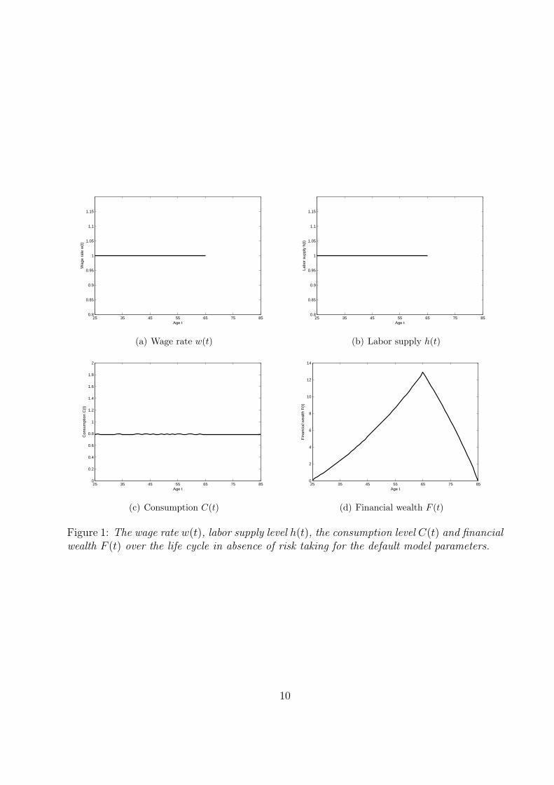
Figure 1: The wage rate w(t), labor supply level h(t), the consumption level C(t) and financialwealth F (t) over the life cycle in absence of risk taking for the default model parameters.

10

for all t0 ≤ t ≤ T . It follows from equation (3.3) that consumption levels are increasing over

the life-cycle if the interest rate r is larger than the individual’s rate of time preference β

and decreasing in the opposite case. The extent to which this difference affects the slope

of the consumption profile is determined by the willingness of the individual to substitute

consumption over time intertemporally, i.e. the elasticity of intertemporal substitution of

consumption 1/γ.

Figure 1 illustrates optimal decision making in absence of risk taking for the default pa-

rameters. The default interest rate is equal to the default rate of time preference, resulting

in a flat consumption profile. During the working period, the labor income of the individual

exceeds the consumption level, such that the individual has positive savings. These sav-

ings result in the accumulation of financial wealth, required to finance consumption in the

retirement period during which there are no labor earnings. Labor earnings are flat over

the working life due to the absence of distortions in labor supply decisions in the individual

retirement savings scheme.

In the presence of risk taking, the optimal investment rule is characterized by the property

that the optimal amount X(t) invested in stocks at age t equals a fixed fraction λ/(γσ) of

the sum of financial wealth F (t) and human wealth H(t):

X(t) =λ

γσ(F (t) + H(t)) (3.4)

for all t0 ≤ t ≤ T , where the human wealth H(t) of the individual at age t represents the

market value of future labor earnings:

H(t) =

{Et

[∫ R

tM(s)M(t)

w(t)h(t)ds]

for t0 ≤ t < R

0 for R ≤ t ≤ T(3.5)

where labor supply levels h(t) are given by equation (2.6).

The consumption profile becomes stochastic in the presence of risk taking and is char-

acterized by the way in which financial shocks are smoothed over consumption levels. In

the optimal consumption rule, a financial shock at time t is levied proportionally on all con-

sumption levels in the remaining lifetime, such that shocks to remaining consumption levels

11

25 35 45 55 65 75 850

5

10

15

20

25

30

Age t

Hum

an w

ealth

H(t

)

(a) Human wealth H(t)

25 35 45 55 65 75 85−5

0

5

10

15

20

25

Time t

Fin

anci

al w

ealth

F(t

)

(b) Financial wealth F (t)

25 35 45 55 65 75 850

1

2

3

4

5

6

7

Age t

Am

ount

inve

sted

in s

tock

s X

(t)

(c) Investments in risky assets X(t)

25 35 45 55 65 75 85

0.8

1

1.2

1.4

1.6

1.8

2

Age t

Con

sum

ptio

n C

(t)

(d) Consumption C(t)

Figure 2: The 90% confidence interval (solid lines) and an example scenario path (dottedline) for human wealth H(t), financial wealth F (t), investments in risky assets X(t) andconsumption C(t).

12

are proportional to the wealth shock:

∂C(s)/C(s)

∂Z(t)=

∂W (t)/W (t)

∂Z(t)=

λ

γ(3.6)

for all t0 ≤ t < s ≤ T . The investment strategy in equation (3.4) causes relative changes

in consumption levels with respect to economic shocks to be independent of age and to be

increasing in the risk premium λ and decreasing in the parameter of risk aversion γ.

Figure 2 illustrates the optimal individual solution in the presence of risk taking. The

figure shows 90% confidence intervals (solid lines) as well as an example scenario path (dotted

line) for several variables. The figure illustrates that the optimal amount invested in stocks

is well above financial wealth levels during the beginning of the life cycle, such that the

individual has to borrow substantial amounts to get the optimal exposure to stock market

risk. This is the result of the fact that young individuals posses little financial capital in

comparison to the value of their human capital. The resulting short position in stocks results

in the possibility of negative values for financial wealth. Future labor earnings are used to

repay loans at a later stage in the working life. The amount of wealth that can be put at

risk through investments in stocks is therefore limited by the market value of human wealth:

X(t) < H(t) (3.7)

The optimal investment strategy thus requires the human capital of the individual to be used

as a collateral to ensure that the loan is paid back. Since short positions in the investment

portfolio are often difficult to implement for individual investors, the next subsection treats

the optimization problem under a borrowing constraint.

4 The individual investor

4.1 The optimization problem

Adverse selection and moral hazard cause borrowing against future labor income often to

be not possible for individual investors. Financial institutions are unable or unwilling to use

human capital as a collateral to ensure that the loan is paid back. This subsection therefore

13

25 35 45 55 65 75 850

1

2

3

4

5

6

7

Age tIn

vest

men

ts in

sto

cks

X(t

)

Figure 3: 90% confidence intervals for investments in risky assets X(t) in presence of theborrowing constraint (solid lines) and in absence of the borrowing constraint (dotted lines).

discusses the optimal solution under an exogenous borrowing constraint:

F (t) ≥ 0 (4.1)

for all t0 ≤ t ≤ T . The borrowing constraint implies that the amount invested in stocks

cannot exceed the financial wealth of the individual:

X(t) ≤ F (t) (4.2)

for all t0 ≤ t ≤ T .

4.2 The optimal solution

Figure 3 illustrates that the borrowing constraint is binding during the beginning of the life

cycle when little financial wealth has been accumulated. The borrowing constraint thereby

causes the exposure to stock market risk for young individuals below the optimal exposure.

This reduction in the risk-bearing capacity of the individual comes at substantial welfare costs

because the individual investor is unable to optimally take advantage of the risk premium

in the financial market. Welfare costs are expressed in terms of the percentage reduction in

the certainty equivalent consumption level, i.e. the certain consumption level that yields an

equivalent welfare level. The borrowing constraint results in a welfare loss of 2.8%, a result

that stresses the importance of the optimal equity exposure during the beginning of the life

cycle of the individual.

14

5 The pension fund policy

5.1 The optimization problem

The objective function of the pension fund is to maximize the utility of the participant.

The investment opportunities of the pension fund are those introduced in subsection 2.1 and

the life cycle characteristics and the preferences of the participant are those introduced in

subsections 2.2 and 2.3 respectively. The model for the pension fund abstracts from wealth

transfers between participants, such that the model features intergenerational risk sharing

nor intragenerational risk sharing. This allows me to focus on a single participant, thereby

greatly reducing the complexity of the model and allowing me to stick close to the analysis

in sections 3 and 4.

I assume that participants are unable to save or borrow outside the pension fund, such

that consumption levels during the working period are given by labor earnings after pension

contributions and consumption levels in the retirement period are given by pension benefits:

C(t) =

{(1− π(t))h(t)w(t) if t0 ≤ t < R

b(t) if R ≤ t ≤ T(5.1)

where π(t) represents the contribution rate and is defined as the faction of labor earnings

pledged to the pension fund during the working period and where b(t) represents the rate at

which pension benefits are received by the individual at age t in the retirement period. The

contribution rate π(t) and benefit rate b(t) are decision variables of the pension fund.

Whereas there is only a single retirement savings account in the individual model of

section 4, there are two accounts in the pension fund model treated in this section. First,

there is the individual account A(t) of the participant, which I will also refer to as the value

of pension accumulations of the individual. Second, there is a collective account S(t) which

the participant does not consider to be his or her own wealth. The collective account is

also referred to as the funding surplus (if S(t) is positive) or the funding shortfall (if S(t) is

negative). The motivation for the introduction of two accounts is the observation that the

value of the liabilities of a pension fund (i.e. the value of pension entitlements accumulated

by participants) is in general unequal to the value of the assets. Deviations between the value

15

of assets and liabilities result in a funding shortfall or a funding surplus. The ownership of

the surplus of a pension fund is typically ambiguous. Moreover, the information fairs that

are provided to pension fund participants typically contain information about the value of

individual pension entitlements only. It is therefore assumed that the participant only takes

into account mutations in the value of pension accumulations when determining labor supply

decisions.

It is often legally or politically not possible for pension funds to provide their participants

with pension entitlements that have a negative value and it is therefore imposed that the

value of pension entitlements is not allowed to become negative:

A(t) ≥ 0 for all S ≤ t ≤ T (5.2)

The budget constraints of the two accounts of the pension fund participant are given by

dA(t) =

{(rA(t) + σλXA(t))dt + σXA(t)dZ(t) + α(t)w(t)h(t)dt if t0 ≤ t < R

(rA(t) + σλXA(t))dt + σXA(t)dZ(t)− b(t)dt if R ≤ t ≤ T(5.3)

and

dS(t) =

{(rS(t) + σλXS(t))dt + σXS(t)dZ(t) + (π(t)− α(t))w(t)h(t)dt if t0 ≤ t < R

0 if R ≤ t ≤ T

(5.4)

where A(t0) = S(t0) = A(T ) = S(T ) = 0. XA and XS represent the amounts invested in

stocks on respectively the individual account A(t) and the collective account S(t) and are

both decision variables of the pension fund. Furthermore α(t) denotes the accrual rate at

time t and is defined as the partial derivative of the value of pension accumulations A(t) at

time t with respect to labor supply level h(t) at time t. Notice that α(t) represents not only

the absolute amount accrued per unit of labor supply on the individual account A(t) but also

the market value of these pension accruals7 because the return on pension accumulations

A(t) is fair in market terms for all t0 ≤ t ≤ T . Future investment decisions thus do not

affect the market value of pension rights accrued at present since the pension fund cannot

create or destroy market value by investing in the financial market.

7In practice there may not be a uniquely defined market price of pension accruals. Pension funds typicallyoffer benefit payments that are linked to inflation or wage levels and therefore cannot be replicated infinancial markets. Additionally, pension funds may offer incomplete contracts to their participants in whichthe pension fund board can exercise discretion in choosing how policy rules are applied.

16

Deviations between contribution rates and accrual rates induce a wage differential : the

effective wage rate against which labor is supplied by the participant is affected by the

pension fund policy. Equation (2.6) suggests that the labor supply level of a pension fund

participant is approximately8 given by

h(t) ≈ (w(t)(1− π(t) + α(t)))ε (5.5)

for all t0 ≤ t < R, where w(t)(1−π(t)+α(t)) represents the effective wage rate of a pension

fund participant per unit of labor supply: labor earnings minus pension contributions plus

the value of pension accruals.

The essential difference between risk taking on the individual account A(t) and risk taking

on the collective account S(t) is the way in which the resulting gains and losses are levied

upon the participant. The gains and losses from risk taking on the individual account A(t)

are levied directly upon the value of pension entitlements and do therefore not affect the

marginal effective wage rate against which labor is supplied. On the other hand, gains and

losses from risk taking on the collective account have to be recouped upon the participant

later in the working life by adjustments in the contribution and the accrual rate. If the

contribution rate exceeds the accrual rate, the pension fund levies a net tax on the labor

earnings of the participant such that a funding shortfall is recouped upon the participant. In

the opposite case a net subsidy is provided on labor earnings such that a funding surplus is

gradually reduced. The mechanism by which funding surpluses and shortfalls are recouped

on participants is referred to as the recovery policy of the pension fund.

From equation (5.4) it follows that the market value of the financial surplus equals the

market value of future net taxes or net subsidies on labor earnings at all times:

S(t) =

{∫ R

tEt

[M(s)M(t)

w(t)h(t) (α(s)− π(s))]ds if t0 ≤ t < R

0 if R ≤ t ≤ T(5.6)

All financial gains and losses that are incurred on the collective account must be recouped

upon the participant during the working period, i.e. S(t) = 0 for all t0 ≤ t < R, since no

labor is supplied by the participant during the retirement period. Furthermore, the absence

8The expression in equation (5.5) is only an approximation for labor supply decisions because the utilityvalue of pension accruals only coincides with the corresponding market value in the first-best solution.

17

of intragenerational and intergenerational transfers implies that the ex ante market value of

pension contributions is equal to the ex ante market value of pension accruals:

E0

[∫ R

0

M(t)

M(0)w(t)π(t)dt

]= E0

[∫ R

0

M(t)

M(0)w(t)α(t)dt

](5.7)

The model feature that the recovery policy induces a wage differential is the result of the

fact that it is imposed that the marginal net tax or net subsidy levied by the pension fund

upon labor supply equals the average net tax or net subsidy. If financial gains and losses

incurred on the collective account were to be levied upon the participant through lump-sum

transfers, no labor supply distortions would be induced. Labor supply distortions exist in

the pension fund model due to the fact that gains and losses from the collective account are

levied on the participant through taxes and subsidies that are proportional to labor supply.

The optimization problem of the pension fund is to maximize the utility of the participant

as given by equation (2.4) with respect to the variables { π(t), α(t), XA(t), XS(t) } during

the working period and { b(t), XA(t) } during the retirement period under the constraints

in equations (5.2), (5.3) and (5.4).

If the labor supply of the participant is elastic (i.e. ε > 0) there exists no analytical

solution for the optimal decision rules. The problem is therefore solved using numerical

methods described in Appendix A.

5.2 The optimal policy

5.2.1 Special case: infinite elastic labor supply (ε = ∞)

If the labor supply choice of the individual is infinitely elastic, then no more risk can be

taken on the collective account S(t) anymore, i.e. XS(t) = 0 for all t0 ≤ t ≤ T . After all,

a positive exposure to stock market risk can result in a funding shortage which needs to be

recouped on the participant trough a net tax on labor supply. This becomes impossible as

the labor supply elasticity goes to infinity.

In absence of risk taking on the collective account, the model for the pension fund cor-

responds to the model for the individual investor under the borrowing constraint as treated

in section 4. The risk-bearing capacity of the pension fund equals that of the borrowing

18

30 40 50 60 70 800

1

2

3

4

5

6

7

Age tIn

vest

men

ts in

sto

cks

X(t

)

Figure 4: 90% confidence intervals for financial wealth XA(t) (dashed lines) and XS(t) (solidlines). Together, the amount invested in stocks by the pension fund sums up to the first-bestallocation of the unconstrained individual (dotted lines).

constrained individual investor and the welfare loss relative to the first-best strategy is equal

to 2.8%.

5.2.2 Special case: inelastic labor supply (ε = 0)

In the case where the labor supply of the participant is inelastic with respect to the wage

differential, the surplus can be freely used by the pension fund without any distortions being

induced. Labor supply levels are at all times equal the first-best labor supply level in the

unconstrained individual solution h(t) = h∗(t), where h∗(t) is defined by equation (2.6).

Absence of distortions implies that the full human wealth of the individual can be used as

collateral by the pension fund through investments on the collective account:

−S(t) > H(t) (5.8)

Gains and losses incurred on the collective account are levied upon the participant through

taxes and subsidies on labor earnings that are non-distortionary. The pension fund has

the same risk-bearing capacity as the unconstrained individual investor and the first-best

strategy can be perfectly replicated by the pension fund.

Figures 4 and 5 illustrate how the first-best consumption and investment rules are per-

fectly replicated by the pension fund policy. In the beginning of the working life, risk is

19

30 40 50 60 70 800

5

10

15

20

25

Age t

Acc

umul

atio

ns A

(t)

(a) Accumulations A(t)

25 35 45 55 65 75 85−4

−3

−2

−1

0

1

2

3

4

5

Age t

Sur

plus

S(t

)

(b) Financial surplus S(t)

25 35 45 55 65 75 85−0.5

−0.4

−0.3

−0.2

−0.1

0

0.1

0.2

0.3

0.4

Age t

Con

trib

utio

n ra

te π

(t)

(c) Contribution rate π(t)

30 40 50 60 70 80−0.4

−0.3

−0.2

−0.1

0

0.1

0.2

0.3

0.4

Age t

Acc

rual

rat

e α(

t)

(d) Accrual rate α(t)

25 35 45 55 65 75 850.85

0.9

0.95

1

1.05

1.1

1.15

1.2

1.25

Age t

Effe

ctiv

e m

argi

nal w

age

rate

1 −

π(t

) +

α(t

)

(e) Effective wage rate 1− π(t) + α(t)

25 35 45 55 65 75 850.8

0.85

0.9

0.95

1

1.05

1.1

1.15

Age t

Labo

r su

pply

h(t

)

(f) Labor supply h(t)

Figure 5: 90% confidence intervals (solid lines) and the example scenario path (dashed line)for pension accumulations A(t), the financial surplus S(t), the contribution rate π(t), theaccrual rate α(t), the effective marginal wage rate 1− π(t) + α(t) and the labor supply levelh(t).

20

taken on the collective account, resulting in a positive or negative financial surplus. The

financial surplus is levied upon the participant in the remaining working life by deviations

between the contribution rate and the accrual rate9 but the resulting wage differential leaves

labor supply unaffected. By perfectly replicating the first-best consumption, investment and

labor supply choices, the pension fund is able to realize the welfare level of the unconstrained

individual investor.

5.2.3 General case: elastic labor supply (0 < ε < ∞)

In this section I discuss the non-trivial case where the labor supply elasticity of the participant

is positive but finite. This implies that risk taking on the collective account S(t) results in

distortions in labor supply decisions, such that it is less attractive to employ the surplus

compared to the case where labor supply is inelastic.

The exposure to stocks that can be realized through risky investments on the collective

account is reduced under elastic labor supply compared to the case of inelastic labor supply.

Whereas the full human wealth can be put at risk under inelastic labor supply, changes in

future earnings induced by the recovery policy have to be taken into account under elastic

labor supply. The maximum revenue η per unit of time (corrected for the wage rate w(t))

that can be pledged from the participant by levying a net taxes on labor earnings is given

by:

ηw(t) ≡ sup−π(t), α(t)

{(−π(t) + α(t))w(t)h(t)} ≈ 1

ε + 1

(ε

ε + 1

)ε

(5.9)

where the approximation for the labor supply choice of a pension fund participant in equation

(5.5) is substituted. From equation (5.9) it follows that the financial surplus is constrained

from below

−S(t) > Et

[∫ R

t

M(s)

M(t)ηw(s)ds

]= ηH(t) (5.10)

where H(t) is the non-stochastic human wealth at time t of the individual investor as defined

by equation (3.5). The constraint in equation (5.10) implies that the exposure to stock

9Introducing intergenerational risk sharing to the model would cause confidence intervals for wage dif-ferentials to become more uniformly distributed over the working life because young workers share in theeconomic shocks that occurred before their time of entrance.

21

0 0.5 1 1.5 2 2.50

0.1

0.2

0.3

0.4

0.5

0.6

0.7

0.8

0.9

1

Labor supply elasticity ε

Fra

ctio

n of

hum

an w

ealth

that

can

be

used

as

colla

tera

l η

Figure 6: The fraction η of human capital that can be put at risk for various parameterchoices for labor supply elasticity ε.

market risk that can be attained through investments in stocks on the collective account is

limited by

XS(t) < ηH(t) (5.11)

It follows from equation (5.9) that positive finite levels of labor supply elasticity (0 < ε <

∞ imply that parameter η is larger than zero but strictly smaller than unity, such it follows

from comparing equations (3.7) and (5.11) that elastic labor supply implies a reduction in

the maximum amount of risk that can be attained through the collective account. Figure 6

illustrates the percentage reduction 1− η% in this maximum amount for various parameter

choices for labor supply elasticity ε. If the parameter of labor supply elasticity ε equals

1.0, the maximum amount that can be put at risk reduced by more than 70%. The case of

infinite labor supply distortions (ε = ∞) results in the situation where the human capital of

the individual cannot be used as collateral at all (η = 0) and in the case where labor supply

distortions are absent (ε = 0) the constraints in equations (3.7) and (5.11) coincide.

Figure 7 shows confidence intervals in the presence of labor supply distortions with ε = 1

(solid lines) and in absence of labor supply distortions, i.e. ε = 0 (dotted lines). Labor

supply distortions cause the amount invested in stocks to decline, especially during the

beginning of the working life where stock investments have to be taken on the collective

account because little financial accumulations have been accumulated. In the presence of

distortions it becomes less attractive to take risks on the collective account, resulting in

smaller wage differentials and smaller funding surpluses and shortfalls compared to the case

22

20 30 40 50 60 70 80 900

1

2

3

4

5

6

7

Age t

Inve

stm

ents

in s

tock

s X

A(t

) +

XS(t

)

(a) Investments in stocks XA(t) + XS(t)

25 30 35 40 45 50 55 60 65−3

−2

−1

0

1

2

3

4

5

Age tS

urpl

us S

(t)

(b) Financial surplus S(t)

25 30 35 40 45 50 55 60 650.85

0.9

0.95

1

1.05

1.1

1.15

1.2

1.25

Time t

Effe

ctiv

e m

argi

nal w

age

rate

1

− π

(t)

+ α

(t)

(c) Effective wage rate 1− π(t) + α(t)

25 30 35 40 45 50 55 60 650.85

0.9

0.95

1

1.05

1.1

1.15

1.2

1.25

Time t

Lab

or s

uppl

y le

vel h

(t)

(d) Labor supply h(t)

Figure 7: 90% confidence intervals for stock investments XA(t)+XS(t), the financial surplusS(t), the effective wage rate 1 − π(t) + α(t) and labor supply levels h(t) in the presence oflabor supply distortions with ε = 1 (solid lines) and in absence of labor supply distortions,i.e. ε = 0 (dotted lines).

23

25 35 45 55 65 75 85−7

−6

−5

−4

−3

−2

−1

0

Time t

5% q

uant

ile o

f Sur

plus

S(t

)

η H(t)

Figure 8: 5% quantile of the financial surplus S(t) (solid line) and the constraint in equation(5.10) (dashed line) if ε = 1.

where distortions are absent. The constraint in equation (5.11) turns out not to hardly

constraining for the default parameter ε = 1, as is illustrated in Figure 8. That is: the

unconditional probability that the constraint in equation (5.11) is binding is negligible. Only

at levels of the parameter of labor supply elasticity ε above 1.5 the unconditional probability

of hitting the constraint becomes substantial.

The intuition for the decline in stock investments reported in Figure 7 can be understood

a comparison to the results of Bodie, Merton, and Samuelson (1992), who find that income

effects in labor supply have a stabilizing effect on the wealth and increase the appetite

for risk taking. The substitution effects in labor supply induced by the recovery policy

work in exactly the opposite direction. Labor supply is decreased after a negative wealth

shock, whereas it is increased after a positive shock. The substitution effects thus trigger

destabilizing wealth effects by causing labor earnings to become more positively correlated

to stock returns, thereby reducing the appetite for risk taking in the investment portfolio

of the pension fund participant. Human capital thus becomes more stock-like rather than

bond-like. This result is consistent with the findings of Cocco, Gomes, and Maenhout (2005),

who show that the optimal exposure to stock returns is reduced as the human capital of an

investor becomes more strongly correlated to stock returns. The reduction in investments in

stocks is economically substantial: for a pension fund with a population that is uniformly

distributed in age, the asset allocation decreases from 44% to 39% as a result of labor supply

24

0 0.5 1 1.5 2 2.5

−3.0%

−2.5%

−2.0%

−1.5%

−1.0%

−0.5%

0

Labor supply elasticity εW

elfa

re lo

ss fr

om la

bor

supp

ly d

isto

rtio

ns First−best welfare level

Welfare level under borrowing constraint

Figure 9: The % change in the the certainty equivalent consumption level (ceteris paribus theleisure level, which is fixed at the levels of the first-best solution given by (2.6) for the cal-culation of the certainty equivalents) over the life cycle for various levels of the compensatedwage-elasticity of labor supply ε.

distortions.

Due to the reduction in the risk bearing capacity, the pension fund participant cannot

take full advantage of the risk premium on financial markets, thereby reducing ex ante welfare

levels. Figure 9 shows, for various levels of the elasticity of labor supply ε, the welfare of

pension fund participation compared to the first best strategy. The model suggests that the

welfare loss for the default parameter of the elasticity of labor supply (ε = 1.0) is around

0.8% which is roughly a third (0.8/2.8 ≈ 1/3) of the welfare gain that recovery policies

generate by enabling individuals to borrow against human capital. Thus, although exposing

human capital through recovery policies remains welfare improving for the participant, its

attractiveness substantially reduces if one recognizes that such policies trigger distortions in

labor supply decisions.

The welfare loss of pension fund participation can be reduced to zero if funding surpluses

and shortfalls are levied upon the participant by lump-sum transfers, rather than by transfers

that are proportional to labor supply. My analysis suggests that the welfare gains from

moving to such ’lump-sum recouping’ yields a welfare gain of 0.8%.

25

6 Conclusions

The model developed in this paper suggests that labor supply flexibility plays a different role

collective pension saving scheme than in an individual saving scheme. Our analysis produces

a number of insights:

Labor supply distortions induced by recovery policies reduce the risk bearing capacity of

participants in collective pension plans. If funding shortfalls and surpluses are recouped on

participants through transfers that are proportional to labor supply, then recovery policies

reduce the risk bearing capacity of fund participants. The analysis therefore suggests that

sectors or industries facing labor market competition from employers with actuarially fair

pension plans may need to reduce the risk taking in their pension funds, compared to the

case where there is no such competition.

The welfare costs from recovery policies (labor supply distortions) can amount to a sub-

stantial fraction of the welfare benefits from recovery policies (alleviation of the borrowing

constraint). For a stand alone pension fund with age-independent policy rules I find that

the welfare costs of recovery policies (distortions in labor supply) are substantial, and equal

roughly a third of the welfare benefits of recovery policies (alleviation of the borrowing

constraint) for the default parameters of the model.

Substantial welfare gains can be realized if financial surpluses and shortfalls are recouped

on participants by lump-sum transfers, rather than by transfers that are proportional to labor

supply. If financial gains and losses incurred on the collective account are levied upon the

participant through lump sum taxes and subsidies on labor earnings, then no labor supply

distortions are induced by the pension fund anymore and a welfare gain of almost a full

percentage point can be realized..

The main virtue of the present model, its simplicity, is also an important limitation. The

way in which labor supply flexibility has been modeled in our paper is far from the workings

of actual labor markets. A more realistic model would therefore allow limited flexibility in

the possibilities of varying intertemporal labor and leisure, while on the other hand allowing

for some flexibility in the participation decision and the retirement decision. Additionally, a

26

more advanced model would recognize risk sharing by the employer and the possibility for

participants to switch jobs to companies or industries with actuarially fair retirement saving

schemes.

This paper underscores the importance of distortionary labor supply effects of recovery

policies of pension funds. This simple observation, however, suggests others. First, it is still

unclear from the current analysis whether labor supply flexibility is a blessing or a curse for a

participant in a collective pension plan. In other words: it is unclear under which conditions

the stabilizing income effects in labor supply are larger or smaller than the destabilizing

substitution effects induced by the recovery policy. Secondly, our findings suggest that the

attractiveness of risk sharing between non-overlapping generations reduces if one recognizes

that the policies that implement such risk sharing facilities come to together with an increase

in labor supply distortions. While the current work on risk sharing between non-overlapping

generations (Gollier (2007)) finds that more risk sharing is always better, the optimal level

of risk sharing will be bounded when labor supply effects are taken into account.

References

Alesina, A., E. Gleaser, and B. Sacerdote (2005): “Work and leisure in the U.S.

and Europe, why so different?,” Harvard Institute of Economic Research, Discussion Paper

Number 2068.

Blundell, R., and T. MaCurdy (1999): “Labor Supply: A Review of Alternative Ap-

proaches,” in: O. Ashenfelter and D. Card (eds.), Handbook of Labor Economics Vol 3A,

Amsterdam: Elsevier North Holland, pp. 1559-1695.

Bodie, Z., R. Merton, and W. Samuelson (1992): “Labour supply flexibility and

portfolio choice in a life cycle model,” Journal of Economics: Dynamics and Control, 16,

427.

Bovenberg, A., T. Nijman, C. Teulings, and R. Koijen (2007): “Saving and invest-

ment over the life cycle: the role of individual and collective pensions,” De Economist,

2007, 155(4), pp. 347-415.

27

Choi, K., G. Shim, and Y. Shin (2008): “Optimal portfolio choice, consumption-leisure

and retirement choice problem with CES utility,” Mathematical Finance, 18, 445.

Cocco, J., F. Gomes, and P. Maenhout (2005): “Consumption and Portfolio Choice

over the Life Cycle,” Review of Financial Studies 18.

Cui, J., F. de Jong, and E. Ponds (2007): “The value of intergenerational transfers

within funded pension schemes,” under review of third submission for Journal of Public

Economics.

Cvitanic, J., L. Goukasian, and F. Zapatero (2007): “Optimal risk taking with

flexible labor income,” Management Science, No. 10, pp. 1594-1603.

Eissa, N., and J. Liebman (1996): “Labor Supply Response to the Earned Income Credit,”

Quarterly Journal of Economics 61, pp. 605-637.

Farhi, E., and S. Panageas (2007): “Saving and investing for early retirement: A theo-

retical analysis,” Journal of Financial Economics 83, pp 87-121.

Gollier, C. (2007): “Intergenerational Risk-Sharing and Risk-Taking of a Pension Fund,”

Journal of Public Economics, Volume 92, pp. 1463-1485.

Gomes, F., J. Kotlikoff, and L. Viceira (2008): “Optimal Life-Cycle Investing with

Flexible Labor Supply, A Welfare Analysis of Life-Cycle Funds,” American Economic

Review, Papers and Proceedings, Vol. 98, pp. 297-303.

Gomes, F., and A. Michaelides (2007): “Optimal Life-Cycle Asset Allocation: Under-

standing the Empirical Evidence,” Journal of Finance, vol 60, pp. 869-904.

Greenwood, J., Z. Hercowitz, and G. Huffman (1988): “Investment, capacity util-

itzation, and the real business cycle,” American Economic Review 78, pp. 402-417.

Heckman, J. (2003): “What has been learned about labor supply in the past twenty

years?,” AEA Papers and Proceedings 83, 116-121.

Merton, R. (1969): “Lifetime portfolio selection under uncertainty, the continuous time

model,” Review of Economics and Statistics, 51, 247.

28

Meyer, B., and D. Rosenbaum (2001): “Welfare, the Earned Income Tax Credit and the

Labor Supply of Single Mothers,” Quarterly Journal of Economics 66, pp. 1063-1114,.

Rauh, J. (2006): “Investment and Financing Constraints: Evidence from the Funding of

Corporate Pension Plans,” The Journal of Finance.

Saez, E. (2002): “Optimal Income Transfer Programs: Intensive Versus Extensive Labor

Supply Responses,” Quarterly Journal of Economics, 117, 1039-1073.

Samuelson, P. (1969): “Lifetime portfolio selection by dynamic stochastic programming,”

Review of Economics and Statistics.

Teulings, C., and C. de Vries (2006): “Generational Accounting, Solidarity and Pension

Losses,” De economist, vol 154, pp 63-83.

Viceira, L. (2001): “Optimal Portfolio Choice for Long-Horizon Investors with Nontradable

Labour Income,” Journal of Finance 56, pp 433-470.

A Numerical solution method

If labor supply is elastic with respect to the wage level (i.e. if ε > 0) then there exists no

analytical solution for the decision rules of the pension fund. The problem is therefore solved

on the basis of numerical methods. During the working period the problem contains two

state variables (A(t) and S(t)) while during the retirement period, in which the financial

surplus is zero, A(t) is the only state variable. I assume that the labor supply decision h(t)

of the pension fund participant is given by the approximation rule given in equation (5.5),

such that there are four decision variables to be solved during the working period (π(t), α(t),

XA(t) and XS(t)) and two decision variables during the retirement period (b(t) and XA(t)).

I apply a discretization with respect to age as well discretization in both dimensions of the

state space. The decision rules can now be represented on a numerical grid in the state space

at all ages t on the age grid. I apply an exponentially spaced in A(t)-dimension, resulting in

relatively many gridpoints at low values of A(t). The state space is bounded from below in

29

the A(t)-dimension as well as in the S(t)-dimension as a result of the constraints in equations

(5.2) and (5.10) respectively.

The decision rules are solved via backward induction. For every age age t on the grid prior

to age T , and for each point in the state space, I optimize utility at time t with respect to the

decision variables using a grid search. Discretization of the utility function with respect to

age implies that utility U(t) at age t is given by the sum of utility gained at the present age t

(∆tu(C(t), h(t)) and the discounted expected continuation value e−β∆tEt [U(t + ∆t)]. Utility

gained from present consumption and leisure follows directly from the decision variables,

whereas the expected continuation value can be computed once the problem at time t + ∆t

is solved. If continuation values do not lie on the the state space grid, I evaluate the value

function on the basis of cubic interpolation of the value function. In the last period the

solution is trivial since the individual finds it optimal to consume all remaining wealth due to

the absence of a bequest motive. This thus gives me the terminal condition for my backward

induction procedure. I perform all numerical integrations using Gaussian quadrature to

approximate the distributions of the innovations to the risky asset return.

The 90% confidence intervals reported in the paper are generated by Monte-Carlo simu-

lations on the basis of the numerically solved decision variables. If the simulated values for

the state variables do not lie on the the state space grid, decision making is evaluated on the

basis of cubic interpolation of decision rules represented on the state space grid.

30