labor productivity, capital accumulation, and aggregate ... · in labor productivity is explained...
TRANSCRIPT

Munich Personal RePEc Archive
Labor productivity, capital accumulation,
and aggregate efficiency across countries:
Some stylized facts
Mendez-Guerra, Carlos
Kyushu University
7 November 2017
Online at https://mpra.ub.uni-muenchen.de/82461/
MPRA Paper No. 82461, posted 08 Nov 2017 00:16 UTC

Labor Productivity, Capital Accumulation,and Aggregate Efficiency across Countries:
Some Stylized Facts
Carlos A. Mendez-Guerra∗
Kyushu University
November 6th, 2017
Abstract
This paper studies the cross-section dynamics of the proximate deter-minants of labor productivity: physical capital, human capital, and aggre-gate efficiency. Using a panel data set for 74 countries covering the 1950-2010 period, it first documents that labor productivity of the median coun-try has been mostly stagnant, while cross-country differences have dras-tically increased. An evaluation of proximate sources points to a similarpattern of stagnation and increasing dispersion in both physical capitaland aggregate efficiency. Human capital is the only variable where medianprogress and inequality reduction can be observed. Next, the paper showshow standard regression methods consistently overestimate the fraction ofthe variation in labor productivity that is explained by physical capital. Thesource of this upward bias appears is the unaccounted covariance betweencapital accumulation and aggregate efficiency. Taking this covariance intoaccount, most of the variation in labor productivity turns out to be ex-plained by differences in aggregate efficiency. Finally, the paper concludesarguing that allocative inefficiencies at the sectoral level, such as those pre-dicted by dual-economy type models, are important for understanding thelarge and increasing differences in aggregate efficiency across countries.
Keywords: labor productivity, capital accumulation, aggregate efficiency,stylized facts
JEL classification: E01, O40, O47
∗Contact Email: [email protected]

2 CARLOS A. MENDEZ-GUERRA
1. Introduction
Arguably, most research studies in the growth and development literature ana-
lyze cross-country differences in labor productivity according to the following
chain of causation (Hsieh and Klenow, 2010):
Figure 1: Cross-Country Differences in Labor Productivity: A Chain of Causality
Geography, Climate, Luck
Institutions, Culture
Policies, Rule of Law, Corruption
Human Capital
Aggregate Efficiency
Physical Capital
Human Capital
Aggregate Efficiency
Physical Capital
Human Capital
Aggregate Efficiency
Physical Capital
Cross-Country Differences in Labor
Productivity
Source: Adapted from Hsieh and Klenow (2010)
Factors that affect labor productivity are typically classified into two groups.
The first includes the most proximate sources such as physical capital, human
capital, and aggregate efficiency. The second includes more fundamental or
deeper determinants such as geography, culture, and institutions and policies.
In the context of Figure 1, this paper analyzes the proximate sources of labor
productivity. First, it quantifies the differences both over time and across coun-
tries of each proximate source. Next, the paper revisits the debate about the
relative importance of capital accumulation versus aggregate efficiency. On the
one hand, the work of Mankiw, Romer, and Weil (1992) uses regression methods
to conclude that capital accumulation differences explain most of the variation
of labor productivity across countries. On the other, the work of Klenow and
Rodriguez-Clare (1997) uses calibration methods to highlight the prevalence
of aggregate efficiency over capital accumulation. On this debate, this paper
emphasizes that the source of disagreements relies on strong conceptual and

LABOR PRODUCTIVITY, CAPITAL ACCUMULATION, AND AGGREGATE EFFICIENCY 3
methodological assumptions of both lines of research. On the one hand, capital
fundamentalists rely on the independence between capital accumulation and
aggregate efficiency to consistently estimate an unbiased OLS regression. On
the other hand, efficiency proponents rely on competitiveness of factor mar-
kets to calibrate key parameters.
After clarifying the relative importance of capital accumulation and aggre-
gate efficiency, this paper discusses a structural change channel through which
some of the deeper determinants described in Figure 1might affect the prox-
imate sources of labor productivity. This channel has to do with the degree
of allocative efficiency across productive sectors within an economy. In par-
ticular, it argues that the degree of misallocation resources across sectors can
potentially have a large negative effect on aggregate efficiency. This observa-
tion is consistent with the dual-economy structures that are typically found
in developing countries (Lewis 1954,1979). Empirically, the work of Vollrath
(2009) shows that degree of resource misallocation between agricultural and
non-agricultural sectors can account for up 80 percent of the cross-country
variation in aggregate efficiency. Finally, the paper provides further evidence on
the dynamics of misallocation. Using the recent sector-level data from McMil-
lan and Rodrik (2011, 2014), this paper presents the case of Chile as an illustra-
tive example in which workers secularly move from relatively high-productivity
sectors to low-productivity sectors.
The rest of the paper is organized as follows. Section 2 describes the evolu-
tion of the cross-country disparities in labor productivity, capital accumulation,
and aggregate efficiency. Section 3 evaluates the relative importance of capital
accumulation and aggregate efficiency. Section 4 presents an structuralist point
of view about the sources of aggregate efficiency. Finally, Section 5 offers some
concluding remarks and open questions for further research.

4 CARLOS A. MENDEZ-GUERRA
2. Labor Productivity its Proximate Sources
Figure 2 shows two key features of the dynamics of labor productivity across
countries. First, contrary to the convergence predictions of the Neoclassical
growth model,1 relative labor productivity of the medium country was almost
stagnant during the 1950-2010 period.2 For instance, in 1950, output per worker
of the median country relative to that in the United States was 22 percent. After
61 years, it decreased to 20 percent.3 Second, the standard deviation increased
from 23 to 32 during this period. That is, productivity differences across coun-
tries increased by a factor of 1.4 during this period. What explains this lack of
convergence and increasing disparities in labor productivity?
Standard growth theory provides the beginning of an answer by organizing
our thoughts around an aggregate production function. For instance, Hall and
Jones (1999) and Caselli (2005, 2014) suggest the following functional form:
Yi = AiKαi (hiLi)
1−α for all α ∈ (0, 1), (1)
where Yi is the total real GDP in country i , Ai represents aggregate efficiency4,
Ki is the total physical capital stock, hi is the human capital per worker, Li is the
total labor force, and α is the elasticity of GDP with respect to physical capital.
Dividing Equation 1 by the labor force Li, and rearranging terms, we can obtain
1See Solow (1956) for details.2Providing some empirical support about the convergence predictions of the Neoclassical
model, Barro (1992) finds conditional convergence across countries after controlling for otherfactors such as fertility, education, population growth, government expenditures, investmentrates, among others. Durlauf, Johnson and Temple (2005), however, criticize this finding argu-ing that the typical convergence regressions implemented in the literature suffer from modeluncertainty, parameter heterogeneity, endogeneity issues, and lack of robustness.
3If in this computation the mean is used, average productivity increased from 33 percent to35 percent. As a measure of centrality, however, the median is typically preferred to the meanwhen a sample contains extremely large or small values.
4The literature typically refers to Ai as total factor productivity (TFP). To avoid confusionwith other productivity terms in this paper I use the term aggregate efficiency instead to totalfactor productivity.

LABOR PRODUCTIVITY, CAPITAL ACCUMULATION, AND AGGREGATE EFFICIENCY 5
Figure 2: Cross-Country Differences in Labor Productivity Over Time
0
20
40
60
80
1950 1960 1970 1980 1990 2000 2010
Year
(USA=100)Relative Output per Worker
Source: Author’s calculations using data from Fernandez-Arias (2014)
an expression for the average productivity of labor:
Yi
Li
= Ai
(Ki
Li
)α
h1−αi . (2)
Equation 2 shows that the (proximate) forces driving the behavior of labor pro-
ductivity can be organized into three variables: aggregate efficiency, physical
capital per worker, and human capital per worker. Alternatively, they can also
be categorized into two factors: aggregate efficiency and capital accumulation,
where the concept of capital in this case includes both physical and human
capita. In any of these classifications the interpretation is equivalent: labor
productivity in country i will be high if its workers accumulate productive re-
sources (e.g., physical capital and human capital) and/or if those resources are
used more efficiently.
Ideally, one would like to use Equation 2 for answering comparative analysis

6 CARLOS A. MENDEZ-GUERRA
questions such as: how much does labor productivity increase in response to an
increase in aggregate efficiency? One problem, however, is that capital accumu-
lation responds endogenously to changes in aggregate efficiency (Klenow and
Rodriguez-Clare, 1997). Conceptually, this endogeneity arises because physical
capital is defined in units of final output. As a result, any increase in aggregate
efficiency would affect labor productivity both directly and indirectly through
capital accumulation. Hsieh and Klenow (2010) argue that keeping physical
capital constant when there is an increase in efficiency requires a decrease in
the investment rate. However, it is not obvious why the investment rate should
decrease to improvements in efficiency. Thus, to deal with the endogeneity is-
sue in a more natural way, Klenow and Rodriguez-Clare (1997) rearrange Equa-
tion2 and suggest the following (steady-state) production function:
Yi
Li
= A1
1−α
i
(Ki
Yi
) α
1−α
hi. (3)
Equation 2 is consistent with the steady state equilibrium of the neoclassical
growth model, where the capital-output ratio, KY , is exogenous to changes in
aggregate efficiency, A. More intuitively, Equation 3 controls for the indirect
effects of improvements in efficiency by raising its elasticity from one to 1
1−α.
Given cross-country data on total production, labor force, physical and hu-
man capital, previous studies have used regression or calibration methods to
empirically implement either equation 2 or 3. In fact, Caselli (2005) and Hsieh
and Klenow (2010) survey the literature that uses calibration methods. In these
surveys, physical capital typically explains around 20 percent, human capital
explains 10 to 30 percent, and aggregate efficiency explains 50 to 70 percent of
the cross-country differences in labor productivity5. Although most economies
would tend to agree with these findings, there are important caveats and lim-
5Originally, Caselli (2005) and Hsieh and Klenow (2010) report cross-country differences inoutput per capita (i.e., differences in income). However, it is well-know that differences in out-put per capita imply differences in output per worker when the employment-to-populationratio does not systematically vary with output per capita.

LABOR PRODUCTIVITY, CAPITAL ACCUMULATION, AND AGGREGATE EFFICIENCY 7
itations. It is also important to analyze why a calibration approach would still
be preferred to a regression-based approach (See section 3.). Before going into
methodological concerns, however, I first discuss the general patterns about
the evolution of the cross-country differences in capital accumulation and ag-
gregate efficiency in the post-World War II period
2.1. Differences in Physical Capital
Long data series on physical capital are not readily available from the national
income accounts of most countries. The standard procedure in the literature
is to build such series by adding investment inflows within an accumulation
framework that includes depreciation outflows. For instance, the Penn World
Tables V.8 database and the database of Fernandez-Arias (2014), which are the
main datasources for this section, uses the perpetual inventory method to con-
struct the physical capital series for 167 countries between 1950 and 2011. This
inventory method requires only two parameters: the depreciation rate and the
initial capital stock. Although the first is typically set to six or ten percent, the
latter is not readily available. Thus, there exist a variety of methods for com-
puting the initial capital stock. For instance, Jones (1997) and Hall and Jones
(1999) use the capital stock in steady state. As described in Caselli (2005), inde-
pendently of the chosen method, initial capital depreciates over time and given
a six percent depreciation rate, the effect of the initial capital would almost dis-
appear after the first 30 years.
Figure 3 shows the two features that characterize the evolution of cross-
country differences in physical capital per worker. First, similar to labor pro-
ductivity, relative physical capital per worker of the medium country was almost
stagnant during the 1950-2010 period. For instance, in 1950, physical capital
per worker relative to that in the United States was 20 percent. After 61 years,
it only increased to 23 percent. Second, cross-country differences in physical
capital are even larger than those in labor productivity. For instance, standard

8 CARLOS A. MENDEZ-GUERRA
Figure 3: Cross-Country Differences in Physical Capital Over Time
0
10
20
30
40
50
60
70
80
1950 1960 1970 1980 1990 2000 2010
Year
Capital-Labor ratio(USA=100)
Source: Author’s calculations using data from Fernandez-Arias (2014)
deviation increased by a factor of 1.6. over the sample period6.
Figure 4 illustrates the strong correlation between labor productivity and
physical capital. Moreover, this correlation appears to become stronger over
time. To further clarify the sources of these results, consider a simplified loga-
rithmic version of Equation 2:
log
(Yi
Li
)
= β + α log
(Ki
Li
)
+ εi. (4)
In this simplified model, cross-country differences in human capital and ag-
gregate efficiency at a point in time would be included in the error term εi.
Moreover, under the strong assumption that these two factors are independent
to physical capital, the elasticity of output per worker with respect to physical
capital, α , could be estimated using a standard OLS regression.
6Specifically, the standard deviation increased from 24 to 39.

LABOR PRODUCTIVITY, CAPITAL ACCUMULATION, AND AGGREGATE EFFICIENCY 9
Given the estimates of Equation 4 and the previously described assumption,
results from Figure 4 would suggest that most of the cross-country variation
in labor productivity is explained by physical capital (the R-squared is close
to one). For instance, in 2010 differences in aggregate efficiency and human
capital would only explain four percent of the differences in labor productiv-
ity. Although the correlation between labor productivity and physical capital
is indeed strong, the reported values for both the capital elasticity and the R-
squared statistic are at odds with those suggested by national accounts (Gollin,
2002). As it will be discussed in Section 3., one can reduce the explanatory
power of physical capital by adding measures of human capital, controlling for
fixed effects, and changing the estimation framework. Yet, before such discus-
sion, let us evaluate how large the differences in human capital are across coun-
tries.
Figure 4: Labor Productivity versus Physical Capital
0
1
2
3
4
5
-2 0 2 4 6
R2 in 2010 = 96%R2 in 1990 = 91%R2 in 1970 = 89%Elasticity in 2010 = [0.84-0.92]
Elasticity in 1990 = [0.72-0.83]
Elasticity in 1970 = [0.66-0.78]
To b
e co
ver
ed i
n w
hit
e
Log (Output per Worker)
Log (Capital-Labor ratio)
Source: Author’s calculations using data from Fernandez-Arias (2014)

10 CARLOS A. MENDEZ-GUERRA
2.2. Differences in Human Capital
The availability of comprehensive cross-country data on human capital seems
be improving every decade. In the early 1990s, growth regressions typically
proxied human capital using measures of school enrollment (Barro and Sala-i-
Martin, 1992; Mankiw et al., 1992). In the late 1990s and early 2000s, growth and
development decompositions (Klenow and Rodriguez-Clare, 1997; Hall and Jones,
1999) typically used measures of years of schooling (from Barro and Lee, 2013)
and the Mincerian return associated to the average years of schooling (from
Psacharopoulos and Patrinos, 2004). More recently, some decomposition stud-
ies started to use measures of the quality of schooling and returns to each year
of work experience (See Kaarsen, 2014; Lagakos et al., 2012 for details).
Figure 5: Cross-Country Differences in Human Capital Over Time
40
50
60
70
80
1950 1960 1970 1980 1990 2000 2010
Year
Human Capital per Worker(USA=100)
Source: Author’s calculations using data from Fernandez-Arias (2014)
Using the human capital production function suggested by Hall and Jones
(1999), Figure 5 shows the two features that characterize the evolution of cross-
country differences in human capital per worker. First, contrasting the pat-

LABOR PRODUCTIVITY, CAPITAL ACCUMULATION, AND AGGREGATE EFFICIENCY 11
terns of both labor productivity and physical capital, relative human capital per
worker of the medium country notably increased during the 1950-2010 period.
After two initial decades of stagnation, human capital accumulation started a
rapid increase. For instance, in 1950, human capital per worker relative to that
in the United States was 54 percent; by 2010 it reached to 74 percent. Second,
cross-country differences in human capital slightly decreased over this period.
For instance, in 1950 the standard deviation was 18 percent; by 2010 it was 16
percent.
Figure 6 shows that human capital is also highly correlated with labor pro-
ductivity, though not as much as physical capital. As in Equation 4, an OLS
regression would suggested that more than 60 percent of the cross-country dif-
ferences in labor productivity are explained by differences in human capital
alone. Again, here the credibility of this explanatory power relies on the strong
assumption that human capital is independent of physical capital and aggre-
gate efficiency.
2.3. Differences in Aggregate Efficiency
Conceptually, aggregate efficiency is a measure that quantifies the efficiency
with which an economy uses its productive resources. Efficiency gains arise due
to improvements in either technical knowledge or reallocation of resources to
better uses (or both). Empirically, aggregate efficiency is a residual measure. It
captures everything else that affects output that is not already measured in the
other inputs (e.g., physical and human capital). According to this definition,
most studies compute aggregate efficiency for a country at a point of time as
the following ratio7:
Ait ≡output
inputs=
Yit
Lit(KL
)αh1−α
. (5)
7See Van Beveren (2012 ) for a practical survey on how to compute aggregate efficiency. Also,see Isaksson (2006, 2007) for an overview of the determinants of aggregate efficiency. Finally,see Felipe, (1999, 2007) for a critical review of the residual approach to aggregate efficiencymeasurement.

12 CARLOS A. MENDEZ-GUERRA
Figure 6: Labor Productivity versus Human Capital
0
1
2
3
4
5
3.5 4 4.5 5
R2 in 2010 = 72%R2 in 1990 = 72%R2 in 1970 = 60%
Elasticity in 2010 = [3.74-5.01]
Elasticity in 1990 = [3.09-4.17]
Elasticity in 1970 = [2.19-3.22]
To b
e co
ver
ed i
n w
hit
eLog (Output per Worker)
Log (Human Capital per worker)
Source: Author’s calculations using data from Fernandez-Arias (2014)
The only missing information to compute this ratio is the output elasticity
with respect to capital, α. Given the results of Figure 4, this parameter tends to
be overestimated when using regression methods. An alternative would be to
extract such information from other sources. For instance, it is well known that
under perfect competition and constant returns to scale, the output elasticity
with respect to capital is defined as the share of national income that accrues to
physical capital. That is
α =rK
Y, (6)
where r is the price of physical capital. Gollin (2002) collects data from dif-
ference sources across countries to construct measures of the capital income
share. After adjusting for the income of self-employed workers, he finds no re-
lationship between the capital share and the level of income per capita (and
labor productivity) across countries (See Figure 7). Moreover, the average cap-
ital share is about 13, which is consistent with the long-run evidence of capital
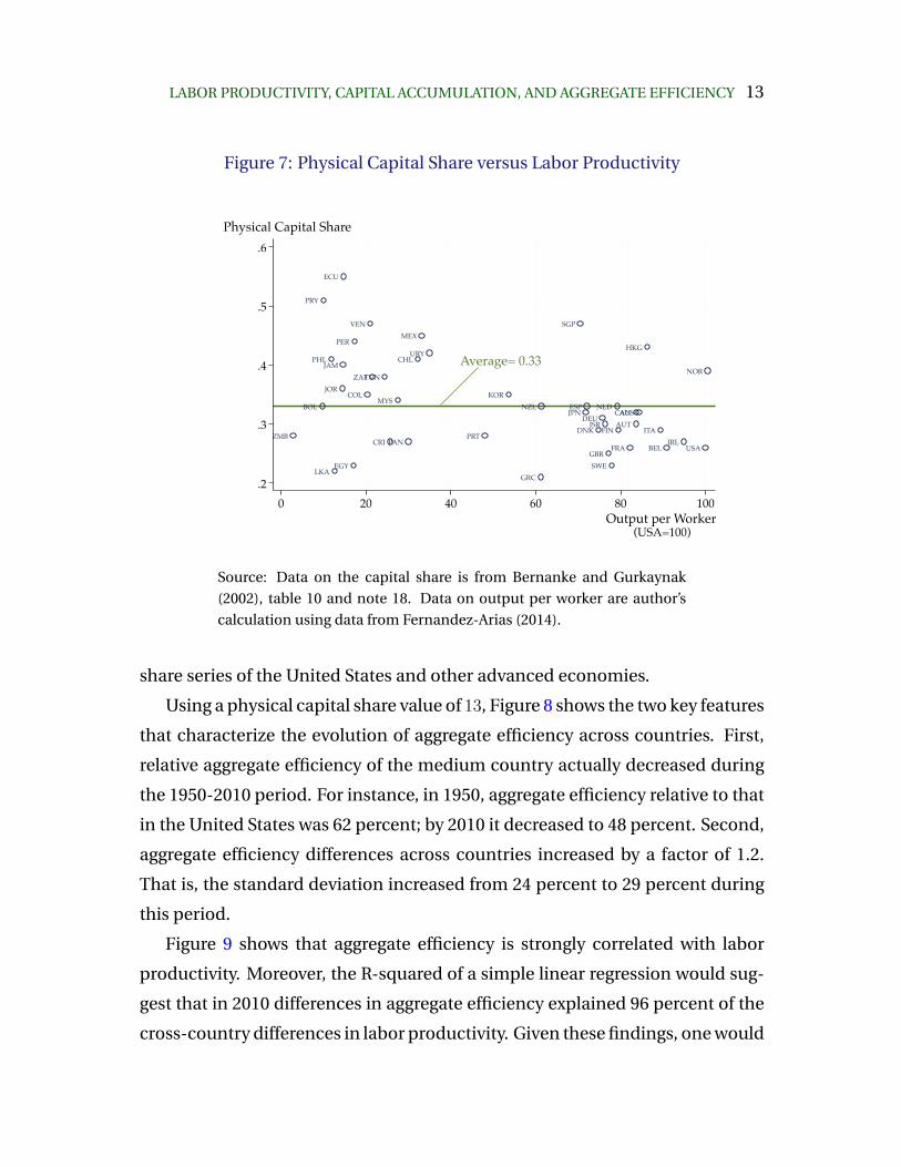
LABOR PRODUCTIVITY, CAPITAL ACCUMULATION, AND AGGREGATE EFFICIENCY 13
Figure 7: Physical Capital Share versus Labor Productivity
AUS
AUT
BEL
BOLCAN
LKA
CHL
COL
CRI
DNK
ECU
FIN
FRA
DEU
GRC
HKG
IRL
ISRITA
JAM
JPN
JORKOR
MYS
MEX
NLDNZL
NOR
PAN
PRY
PER
PHL
PRT
SGP
ZAF
ESP
SWE
TUN
EGY
GBRUSA
URY
VEN
ZMB
Average= 0.33
.2
.3
.4
.5
.6k
shar
e
0 20 40 60 80 100Output per Worker
Physical Capital Share
(USA=100)
Source: Data on the capital share is from Bernanke and Gurkaynak
(2002), table 10 and note 18. Data on output per worker are author’s
calculation using data from Fernandez-Arias (2014).
share series of the United States and other advanced economies.
Using a physical capital share value of 13, Figure 8 shows the two key features
that characterize the evolution of aggregate efficiency across countries. First,
relative aggregate efficiency of the medium country actually decreased during
the 1950-2010 period. For instance, in 1950, aggregate efficiency relative to that
in the United States was 62 percent; by 2010 it decreased to 48 percent. Second,
aggregate efficiency differences across countries increased by a factor of 1.2.
That is, the standard deviation increased from 24 percent to 29 percent during
this period.
Figure 9 shows that aggregate efficiency is strongly correlated with labor
productivity. Moreover, the R-squared of a simple linear regression would sug-
gest that in 2010 differences in aggregate efficiency explained 96 percent of the
cross-country differences in labor productivity. Given these findings, one would

14 CARLOS A. MENDEZ-GUERRA
Figure 8: Cross-Country Differences in Aggregate Efficiency Over Time
20
30
40
50
60
70
80
90
100
1950 1960 1970 1980 1990 2000 2010
Year
Aggregate Efficiency(USA=100)
Source: Author’s calculations using data from Fernandez-Arias (2014)
not only conclude that differences in aggregate efficiency could be as important
as physical capital, but also that these two measures are highly correlated. In
fact, for the year 2010 the pairwise correlation between them was 0.93.
3. Capital Accumulation or Aggregate Efficiency?
The main criticism to the regression approach is that both the elasticity of out-
put with respect to capital (α) and the R-squared tend to be upwardly biased.
The source of this overestimation is the uncontrolled correlation between cap-
ital accumulation and the residual term, which by the definition of Equation 1
represents aggregate efficiency. Additional regression analyses, summarized in
Table 1, suggest that the implausible values for α (and the R-squared) persist af-
ter controlling for human capital, country fixed effects, and constant returns to
scale. As a result, if the correlation between capital and the residual is so strong,

LABOR PRODUCTIVITY, CAPITAL ACCUMULATION, AND AGGREGATE EFFICIENCY 15
Figure 9: Labor Productivity versus Aggregate Efficiency
0
1
2
3
4
5
2 3 4 5
R2 in 2010 = 96%R2 in 1990 = 90%R2 in 1970 = 83%
Elasticity in 2010 = [1.73-1.90]
Elasticity in 1990 = [1.73-2.02]
Elasticity in 1970 = [1.67-2.07]
To b
e co
ver
ed i
n w
hit
eLog (Output per Worker)
Log (Aggregate Efficiency)
Source: Author’s calculations using data from Fernandez-Arias (2014)
how can we identify the variation of labor productivity that is due to capital
differences alone? Consistent with the calibration methodology suggested by
Klenow and Rodriguez-Clare (1997), Vollrath (2014) describes a simple solution
for controlling the previously described correlation.
Let us rewrite the simple econometric model described in Equation 4 as:
log yi = β + α log ki + εi, (7)
where labor productivity y and the capital-labor ratio k are expressed as lower-
case letters just to simplify notation. Then, define the variation of the depen-
dent variable that is explained by the model as:
R2 =V ar (β + α log ki)
V ar (log yi). (8)
Next, utilize the statistical properties of the variance and covariance operators

16 CARLOS A. MENDEZ-GUERRA
Table 1: Different Estimations of Output Elasticities: 1950-2010 Period
Dependent Variable: Labor Productivity
Model (1) Model (2) Model (3) Model (4)
Physical Capital 0.74 0.74 0.59 0.55
(0.01) (0.06) (0.05) (0.01)
Human Capital 0.26 0.26 -0.78 0.45
(0.03) (0.06) (0.14) (0.01)
Fixed Effects NO NO YES YES
Constraint (β1 + β2 = 1) NO YES NO YES
R2 0.90 na 0.84 na
Observations 4284 4284 4284 4284
Note: Numbers in parentheses indicate robust standard errors. All variables aresignificant at 1 percent. All regressions include a constant term that is not re-ported in the table.
and the definition of the OLS estimator to show that
R2 = α2V ar (log ki)
V ar (log yi)
= αCov (log ki, log yi)
V ar (log ki)︸ ︷︷ ︸
α
V ar (log ki)
V ar (log yi)
=Cov (αlog ki, log yi)
V ar (log yi)
=Cov (αlog ki, β + α log ki + εi)
V ar (log yi)
=Cov (αlog ki, β)
V ar (log yi)+
Cov (αlog ki, α log ki)
V ar (log yi)+
Cov (αlog ki, ε)
V ar (log yi)
= 0 +V ar (αlog ki)
V ar (log yi)+
Cov (αlog ki, ε)
V ar (log yi)(9)
Equation 9 shows that we can compute the unbiased R-squared by letting

LABOR PRODUCTIVITY, CAPITAL ACCUMULATION, AND AGGREGATE EFFICIENCY 17
Cov (αlog ki, ε) = 0 and selecting a value for α. Using the results of Figure 7,
most calibration studies set α = 13. Given this setting, in the year 2010 dif-
ferences in physical capital accumulation explain only 14 percent of the differ-
ences in labor productivity across countries. One can also apply the same pro-
cedure for computing the contribution of aggregate efficiency8. For the same
year, differences in aggregate efficiency explain 44 percent of the differences in
labor productivity across countries. This finding is consistent with previous lit-
erature (Baier et al., 2006; Caselli, 2005; Hall and Jones, 1999; Hsieh and Klenow,
2010 ) in the sense that aggregate efficiency is the main driving force behind the
labor productivity.
4. What Explains Aggregate Efficiency? A
Structuralist View
Classical development economics models, such as Lewis (1954), focus on the
coexistence of fundamentally different structures of production within an econ-
omy.9 In its simplest representation, Lewis’ dual economy model conceptual-
izes the process of economic development as the movement of workers from
low productivity sectors (e.g., agriculture) to relatively high productivity sec-
tors (e.g., manufacturing). However, it is possible that some factors of produc-
tion face mobility barriers across sectors. In this case, the economy would suf-
fer from efficiency losses, as factors of production are not reallocated to their
most efficient use.10 Another possibility is that workers (and firms) may have
incentives to move to even lower productivity sectors. For instance, if labor
and product markets are highly regulated, so that operational costs are higher
8Note that in this case Cov (log Ai, ε) = 09See Ross (2000, 2013) for a recent textbook treatment on how to integrate the insights from
classical development economics into modern growth theory.10See Banerjee and Duflo (2005), Hsieh and Klenow (2009), and Restuccia and Rogerson
(2008, 2013) as examples of recent seminal contributions dealing with the relationship betweenresource misallocation and aggregate efficiency.

18 CARLOS A. MENDEZ-GUERRA
in the formal sector, many firms (and the workers they hire) would have addi-
tional incentives to move to the informal sector, where the regulation burden
(and its associated cost) is minimized. The main lesson of this type of models is
that structural productivity differences across sectors have aggregate efficiency
implications.11 In particular, resource misallocation across sectors reduces ag-
gregate efficiency, and ultimately labor productivity.
4.1. Dual-Economy and Misallocation Effects
Figure 10 illustrates how structural productivity differences and resource misal-
location reduces total output. In this example, an economy maximizes its effi-
ciency when the marginal productivity of labor is equal across sectors (MPL1 =
MPL2). At Point D, the economy allocates L∗
1workers to sector one and L∗
2
workers to sector two. The efficiency maximizing level of output is represented
by Y ∗. If there exist market failures or government distortions (or both), wedges
between the marginal products ( MPL1 6= MPL2) will be generated. At point W,
the economy allocates more workers to sector one LM1
and less workers to sec-
tor two LM2
. Given the wedges between marginal products (MPL1 < MPL2),
the efficiency loss in the economy is represented by the DWL triangle and the
new level of output is Y M < Y ∗.
Given the theoretical insights of Figure 10, one would like to have a quantita-
tive measure of the productivity wedges across sectors and their effect on aggre-
gate efficiency. Vollrath (2009) is a seminal contribution in this line of research.
He first constructs agricultural and non-agriculture production functions for
sample of countries in 1985. Then, he calibrates the parameters of each produc-
tion structure to have measures of wedges in marginal productivities between
agriculture and non-agriculture. As expected, marginal productivity differences
tend be larger in developing countries. Figure 11 not only illustrates the original
finding of Vollrath (2009), but it also shows that such inter-sectorial productivity
11See Temple (2005) for a premier treatment on how to integrate dual-economy models intogrowth theory.

LABOR PRODUCTIVITY, CAPITAL ACCUMULATION, AND AGGREGATE EFFICIENCY 19
Figure 10: The Deadweight Loss of Resource Misallocation
Labor allocated to sector 2
Units of output
Labor allocated to sector 1
Marginal product of labor
in sector 1
Marginal product of labor
in sector 2
LM1
LM2
Y*
YM
L*1
L*2
Output lost due to misallocation
DWLD
W
L
Source: Adapted from Weil (2013)
gaps are highly correlated with differences in aggregate labor productivity.
Following the logic of Figure 10, the next step is to compute the DWL triangle
for sample of 42 developed and developing countries. Vollrath (2009) first hy-
pothetically equalizes the the marginal products between agriculture and non-
agriculture for each country. This equalization pins down the optimal alloca-
tion of resources across sectors. Then, using this optimal allocation, he recom-
putes the aggregate production for each country. He finds that resource misal-
location between agriculture and non-agriculture explains up to 80 percent of
the variation in aggregate efficiency and between 30 percent to 40 percent of the
variation in labor productivity. Based on the data of these calculations, Figure
12 shows that countries with the lowest aggregate labor productivity are those
with the largest efficiency losses due to misallocation.

20 CARLOS A. MENDEZ-GUERRA
Figure 11: Dual-Economy Evidence: Large Productivity Gaps across Sectors
Argentina
Australia
Austria
Canada
ChileColombia Costa Rica
Denmark
Dominican Rep.
Egypt
Finland
France
Greece
Guatemala
Honduras
India
Indonesia
Iran
Italy
Japan
Netherlands
New Zealand
Norway
Pakistan
Peru
Philippines
Portugal
South Korea
Sri Lanka
Sweden
Syria
Tunisia
Turkey
United Kingdom
United States
Uruguay
Venezuela
0
20
40
60
80
100
1 2 3 4 5Marginal Product of Labor (non-agriculture)
Economy-wide Labor Productivity
Marginal Product of Labor (agriculture)
(USA=100)
Source: Author’s calculations using data from Vollrath (2009)
4.2. Dynamic Dual-Economy Effects and Structural Change
Figures11 and 12 document the static aggregate efficiency effects of the dual
economy structure. The original insight of Lewis, however, focuses on the dy-
namics of reallocation, that is workers moving from traditional-low-productivity
sectors to modern-high-productivity sectors over time. McMillan and Rodrik
(2011, 2013) aim to extend the research on the dynamics of the dual economy
by constructing a panel dataset that covers a sample of developing and devel-
oped countries for the period 1950-2005. The caveat of this dataset, however,
is that it measures average labor productivity instead of marginal labor produc-
tivity. Note that the conceptual framework illustrated in Figure 10 depends on
the wedges between marginal products, which are not necessarily equal to av-
erage products. In spite of this limitation, one can still try to infer differences in
marginal products from differences in average products. Let us consider both
the average and marginal products of labor in a standard Cobb-Douglass pro-

LABOR PRODUCTIVITY, CAPITAL ACCUMULATION, AND AGGREGATE EFFICIENCY 21
Figure 12: How Large are the Dual Economy Effects?
Argentina
Australia
Austria
Canada
Chile ColombiaCosta Rica
Denmark
Dominican Rep.
Egypt
Finland
France
Greece
Guatemala
Honduras
India
Indonesia
Iran
Italy
Japan
Netherlands
New Zealand
Norway
Pakistan
Peru
Philippines
Portugal
South Korea
Sri Lanka
Sweden
Syria
Tunisia
Turkey
United Kingdom
United States
Uruguay
Venezuela
0
20
40
60
80
100
0 10 20 30 40
Deadweight Loss due to Misallocation
Economy-wide Labor Productivity(USA=100)
Source: Author’s calculations using data from Vollrath (2009)
duction function:
Y = AK1−βLβ (10)
Average Product of Labor ≡Y
L(11)
Marginal Product of Labor ≡∂Y
∂L= β
Y
L. (12)
If the parameter β is relatively constant across sectors and over time, then dif-
ferences in average products will translate into differences in marginal prod-
ucts. Whether this is a valid assumption is a topic for further research. For the
purpose of exploration, and keeping in mind this key assumption, Figure 13
describes the dynamics of the dual economy for a sample country: Chile.
The striking feature of Chile (and Latin America in general) is that the struc-
tural change patterns described in Lewis (1954) appear to be working–in re-

22 CARLOS A. MENDEZ-GUERRA
verse (McMillan and Rodrik, 2011). Over time, workers keep gravitating from
relatively low-productivity sectors (e.g., agriculture and manufacturing) to even
lower-productivity sectors (e.g., wholesale and retail trade, and other services)12.
More generally, McMillan and Rodrik (2013) document the structural change
patterns for sample of developing countries in Latin America, Asia, and Africa.
They conclude that after the year 2000, favorable labor reallocation increased
productivity growth both in Asia and Africa, whereas labor misallocation de-
creased the growth potential of Latin America.
5. Concluding Remarks
A central topic in the study of global development has to do with the huge dif-
ferences in labor productivity across countries. The literature on this topic is
typically classified into two lines of research. One that studies a set of proxi-
mate sources: physical capital, human capital, and aggregate efficiency. And
the other that studies a set of deeper factors: geography, culture, and institu-
tions.
From an empirical point of view, that key motivating fact is that, during the
1950-2010 period, labor productivity of the median country has been mostly
stagnant, while the cross-country differences have drastically increased. An
evaluation of the cross-section dynamics of the proximate sources of labor pro-
ductivity reveals the following patterns:
• Physical capital accumulation in the median country also appears largely
stagnant, with an increasing dispersion in the upper tail over time.
• Aggregate efficiency in the median country decreased over time, with an
increasing dispersion in both upper and lower tails.
12Note that average productivity has been increasing both in the mining sector and in thefinance and business sector. However, the employment share in these sectors is relatively smallcompared to other parts of the economy.

LABOR PRODUCTIVITY, CAPITAL ACCUMULATION, AND AGGREGATE EFFICIENCY 23
Figure 13: Dynamic Dual-Economy Effects: An Example from Chile
.31.65
.28
.11 .2
.3
.4
.5
.6
.7
.1
.15
.2
.25
.3
.35
1945 1955 1965 1975 1985 1995 2005
Agriculture
Share Sectoral/Total
1.83
.05
.01
6.62
2
3
4
5
6
7
.01
.02
.03
.04
.05
.06
1945 1955 1965 1975 1985 1995 2005
Mining
Share Sectoral/Total
.19
.11
1.61
.78 .8
1
1.2
1.4
1.6
.1
.15
.2
.25
1945 1955 1965 1975 1985 1995 2005
Manufacturing
Share Sectoral/Total
3.28
.02
.12
1.20
1
2
3
4
.02
.04
.06
.08
.1
.12
1945 1955 1965 1975 1985 1995 2005
Finance and Busines Services
Share Sectoral/Total
.10
.96
.59
.22
.6
.8
1
1.2
.1
.15
.2
.25
1945 1955 1965 1975 1985 1995 2005
Wholesale and Retail Trade
Share Sectoral/Total
.22
1.48
.26
.61.6
.8
1
1.2
1.4
1.6
.2
.25
.3
.35
1945 1955 1965 1975 1985 1995 2005
Source: Author’s calculations using data from McMillan and Rodrik
(2011)
• Human capital accumulation in the median country increased over time.
Contrasting the behavior of other proximate sources, this is the only vari-

24 CARLOS A. MENDEZ-GUERRA
able in which the cross-country dispersion decreased over time.
From a methodological standpoint, regression methods typically overestimate
the fraction of the variation in labor productivity that is explained by physical
capital. Such overestimation arises from the uncontrolled covariance between
capital accumulation and aggregate efficiency. Calibration methods attempt to
control such covariance and highlight that most of the variation in labor pro-
ductivity is actually explained by aggregate efficiency.
Figure 14 presents an expanded version of the chain of causality suggested
by Hsieh and Klenow (2010)13. The recent empirical literature on resource mis-
allocation across sectors provides new insights on the intermediate channels
between the deep and proximate sources of labor productivity. A large fraction
of the observed deterioration in aggregate efficiency is most likely to be driven
by allocation failures. For instance, the economies of Latin America appear to
be suffering from inefficient sectorial production, since most of their labor force
is concentrated in the service sector, which is the part of the economy where
average productivity is the lowest. Ultimately, resource misallocation is most
likely to be driven by policy failures, institutional weaknesses, and cultural bar-
riers.
Over the next decades, research in economic growth and development is
expected generate new insights based on the potentially fruitful integration of
the recent quantitative dual-economy models and the standard productivity
accounting methods. In this context, some of the major questions for further
analysis may include the following14: In what dimensions the production func-
tion of human capital differs across sectors? What kind of allocative inefficien-
cies have the largest effects? Are the misallocation effects across sectors larger
than those across firms? Under what conditions does a reduction in misalloca-
tion imply an unambiguous gain in welfare? Why is there a secular deterioration
in allocative efficiency in Latin America?
13See Figure 1.14Some of these questions are from Hsieh and Klenow (2010).

LABOR PRODUCTIVITY, CAPITAL ACCUMULATION, AND AGGREGATE EFFICIENCY 25
Figure 14: Cross-Country Differences in Labor Productivity: An Extended Chainof Causality
Geography, Climate,
Luck
Institutions, Culture
Policies, Rule of Law, Corruption
Human Capital
Aggregate Efficiency
Physical Capital
Human Capital
Aggregate Efficiency
Physical Capital
Human Capital
Aggregate Efficiency
Physical Capital
Cross-Country Differences in
Labor ProductivityResource
Misallocation across Sectors
Source: Adapted from Hsieh and Klenow (2010)
References
Baier, S. L., Dwyer, G. P., and Tamura, R. (2006). How important are capital and total
factor productivity for economic growth? Economic Inquiry, 44(1):23–49.
Banerjee, A. V. and Duflo, E. (2005). Growth theory through the lens of development
economics. In Aghion, P. and Durlauf, S. N., editors, Handbook of Economic Growth,
volume 1, Part A of Handbook of Economic Growth, pages 473 – 552. Elsevier.
Barro, R. J. (1991). Economic growth in a cross section of countries. The Quarterly
Journal of Economics, 106(2):407–443.
Barro, R. J. and Sala-i Martin, X. (1992). Convergence. Journal of Political Economy,
100(2):223–251.
Caselli, F. (2005). Accounting for cross-country income differences. In Aghion, P. and
Durlauf, S., editors, Handbook of Economic Growth, volume 1 of Handbook of Eco-
nomic Growth, pages 679–741. Elsevier.
Caselli, F. (2014). The latin american efficiency gap. Discussion Papers 1421, Centre for
Macroeconomics (CFM).

26 CARLOS A. MENDEZ-GUERRA
Durlauf, S. N., Johnson, P. A., and Temple, J. R. (2005). Growth econometrics. In Aghion,
P., editor, Handbook of Economic Growth, volume 1, Part A, pages 555 – 677. Elsevier.
Felipe, J. (1999). Total factor productivity growth in east asia: A critical survey. Journal
of Development Studies, 35(4):1–41.
Felipe, J. and McCombie, J. S. (2007). Is a theory of total factor productivity really
needed? Metroeconomica, 58(1):195–229.
Fernandez-Arias, E. (2014). Productivity and factor accumulation in latin america and
the caribbean: A database (2014 update). Research Department, Inter-American De-
velopment Bank.
Gollin, D. (2002). Getting income shares right. Journal of Political Economy, 110(2):458–
474.
Hall, R. E. and Jones, C. I. (1999). Why do some countries produce so much more output
per worker than others? Quarterly Journal of Economics, 114(1):83–116.
Hsieh, C.-T. and Klenow, P. J. (2009). Misallocation and manufacturing tfp in china and
india. Quarterly Journal of Economics, 124(4):1403–1448.
Hsieh, C.-T. and Klenow, P. J. (2010). Development accounting. American Economic
Journal: Macroeconomics, 2(1):207–223.
Isaksson, A. (2007). Determinants of total factor productivity: A literature review. Re-
search and Statistics Branch, UNIDO.
Isaksson, A. and Ng, T. H. (2006). Determinants of productivity: cross-country analysis
and country case studies. Research and Statistics Branch, Staff Working Paper, 1:2006.
Jones, C. I. (1997). Convergence revisited. Journal of Economic Growth, 2(2):131–153.
Kaarsen, N. (2014). Cross-country differences in the quality of schooling. Journal of
Development Economics, 107:215–224.
Klenow, P. J. and Rodrı́guez-Clare, A. (1997). The Neoclassical Revival in Growth Eco-
nomics: Has It Gone Too Far?, volume 12 of NBER Chapters, pages 73–114. National
Bureau of Economic Research, Inc.

LABOR PRODUCTIVITY, CAPITAL ACCUMULATION, AND AGGREGATE EFFICIENCY 27
Lagakos, D., Moll, B., Porzio, T., Qian, N., and Schoellman, T. (2012). Experience mat-
ters: Human capital and development accounting. NBER Working Paper 18602.
Lewis, W. A. (1954). Economic development with unlimited supplies of labour. The
manchester school, 22(2):139–191.
Lewis, W. A. (1979). The dual economy revisited. The Manchester School, 47(3):211–229.
Mankiw, N. G., Romer, D., and Weil, D. N. (1992). A contribution to the empirics of
economic growth. Quarterly Journal of Economics, 107(2):407–437.
McMillan, M., Rodrik, D., and Verduzco-Gallo, I. n. (2014). Globalization, structural
change, and productivity growth, with an update on africa. World Development,
63:11–32.
McMillan, M. S. and Rodrik, D. (2011). Globalization, structural change and produc-
tivity growth. NBER Working Papers 17143, National Bureau of Economic Research,
Inc.
Restuccia, D. and Rogerson, R. (2008). Policy distortions and aggregate productivity
with heterogeneous establishments. Review of Economic Dynamics, 11(4):707–720.
Restuccia, D. and Rogerson, R. (2013). Misallocation and productivity. Review of Eco-
nomic Dynamics, 16(1):1 – 10.
Ros, J. (2000). Development theory and the economics of growth. University of Michigan
Press, Ann Arbor.
Ros, J. (2013). Rethinking economic development, growth, and institutions.
Solow, R. M. (1956). A contribution to the theory of economic growth. The quarterly
journal of economics, 70(1):65–94.
Temple, J. (2005). Dual economy models: A primer for growth economists. Manchester
School, 73(4):435–478.
Van Beveren, I. (2012). Total factor productivity estimation: A practical review. Journal
of Economic Surveys, 26(1):98–128.

28 CARLOS A. MENDEZ-GUERRA
Vollrath, D. (2009). How important are dual economy effects for aggregate productivity?
Journal of Development Economics, 88(2):325–334.
Vollrath, D. (2014). Is capital important? [Web page] Retrieved from http://growthecon.wordpress.com/2014/04/10/is-capital-important/
Weil, D. N. (2013). Economic growth. Pearson Addison-Wesley, Boston, MA.