Lab 12. Speed Control of a D.C. motor

Controller Design

Motor Speed Control Project

1. Generate PWM waveform2. Amplify the waveform to drive the motor3. Measure motor speed4. Measure motor parameters5. Control speed with a PID controller

ComputerSystem

12v DCMotor

ACTachometer

Amplifier12v

PowerSupply Labs 11/12

SpeedMeasurement

Technical goals for lab

Design a PID controller to regulate the motor speed Design in Simulink Implement in software

Demonstrate improvement in motor performance with the PID controller Faster rise time (50% or more) No steady-state error Minimal overshoot of target speed Fast settling time when changing speeds

Simplified system modelDuty cycle of PWM signal

ADC/Timer output

Switchsetting

Determinedexperimentally

PID algorithm

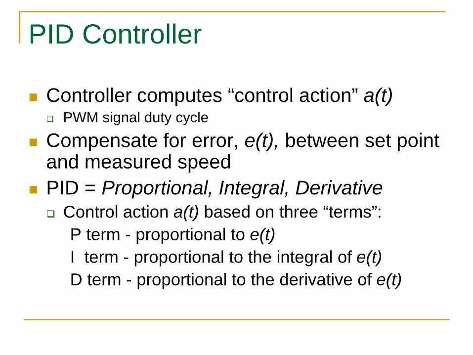
PID Controller

Controller computes “control action” a(t) PWM signal duty cycle

Compensate for error, e(t), between set point and measured speed

PID = Proportional, Integral, Derivative Control action a(t) based on three “terms”:

P term - proportional to e(t)I term - proportional to the integral of e(t)D term - proportional to the derivative of e(t)

PID Controller Design

Continuous time domain:

LaPlace transform/Controller transfer function:

e(t) = error detected at time ta(t) = control action computed at time tKP, KI, KD = constants

dttdeKdtteKteKta D

t

IP)()()()(

0

++= ∫

sKs

KKsEsAsC D

IP ++==

)()()(

PID Controller Design

Discrete time domain:

z transform:

T = sampling timen = sample numbere(nT) = error computed at nth sampling intervala(nT) = control action computed at nth sampling intervalKP, KI, KD = constants

∑=

−−+

−++=

n

iDIP T

TnTenTeKTiTeiTeKnTeKnTa0

)()(2

)()()()(

−

+

−+

+==z

zT

KzzTKK

zEzAzC DIP

1111

2)()()(

Proportional Control

Controller produces a control action that is proportional to the error at any given time

a(t) = Kpe(t) Advantages:

Simple to implement Larger Kp causes greater system response to a given error e(t)

(possibly improve system performance) Disadvantages:

some steady-state error is required to have a control action can overshoot set point and possibly produce unstable behavior controller reacts to high-frequency “noise” in e(t)

Integral Control

Controller produces a control action proportional to the integral of the error (area under the error curve)

This term determines the steady-state control action when e(t)=0 (P and D terms are both 0)

Advantages: eliminates steady state error dampens response to high frequency noise on e(t)

Disadvantages: slows system response can contribute to overshoot

∫=t

I dtteKta0

)()(

Convert integral term to discrete forme(t)

tnT-T nT

e(nT)

e(nT-T)

Consider integral up to previous and current sample times:

incremental areafrom (nT-T) to nT

area up tot = nT-T

Compute the areaunder the curve

∫∫∫−

−

+==nT

TnTI

TnT

I

t

I dtteKdtteKdtteKty )()()()(00

),()()( TnTnTyTnTynTy −∆+−=

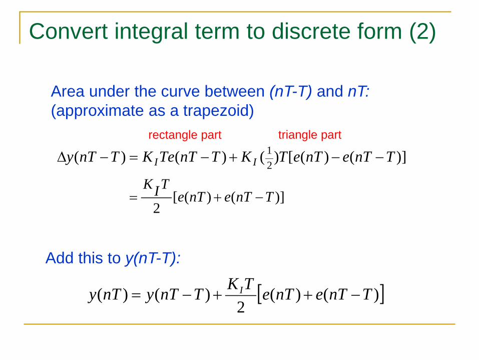
Convert integral term to discrete form (2)

)]()([)()()(21 TnTenTeTKTnTTeKTnTy II −−+−=−∆

Area under the curve between (nT-T) and nT: (approximate as a trapezoid)

)]()([2

TnTenTeTIK

−+=

Add this to y(nT-T):

rectangle part triangle part

[ ])()(2

)()( TnTenTeTKTnTynTy I −++−=

Discrete transfer function of the integral term

Difference equation:

z transform:

Transfer function:

[ ])()(2

)()( TnTenTeTKTnTynTy I −++−=

[ ]11 )()(2

)()( −− ++= zzEzETKzzYzY I

−+

=

−+

= −

−

11

211

2)()(

1

1

zzTK

zzTK

zEzY

II

Derivative control

Controller produces a control action proportional to the derivative of the error anticipates direction of error changes can decrease overshoot can dampen oscillatory behavior BUT: increases sensitivity to high frequency noise in e(t)

Normally, derivative term used only in conjunction with P and/or I terms

The discrete form of the D term:

[ ]y nT Ke nT e nT T

TKT

e nT e nT TDD( )

( ) ( )( ) ( )=

− −

= − −

Compute the slope of e(t) at the current sample time:

[ ]Y zKT

E z E z zD( ) ( ) ( )= − −1

[ ]Y zE z

KT

zKT

zz

D D( )( )

= − =−

−111

Z transform:

Transferfunction:

Implementing the PID controller

)]()([)]()([2

)]2()([)()()()(

TnTenTeT

KTnTenTeTK

TnTeTnTeT

KTnTeKTnTanTeKnta

DI

DPP

−−+−++

−−−−−−−+=

Combine the discrete P, I and D terms:

Consider the previous sample time:

Solve 2nd equation for y(nT-T) and substitute into 1st equation:

[ ] [ ])()(2

)()(2

)()()( TnTenTeKTnTenTeTKTnTynTeKnTa DIP −−+−++−+=

[ ])2()(2

)()()( TnTeTnTeKTnTyTnTeKTnTa DP −−−+−+−=−

Implementing the PID controller (2)

Simplify by combining terms involving e(nT), e(nT-T), e(nT-2T):

)2()()()()( 210 TnTeATnTeAnTeATnTanTa −+−−+−=

A0, A1, A2 are constantse(nT), e(nT-T), e(nT-2T) are the 3 most recent error valuesa(nT-T) is the previous control action

Software procedure at each sample time:•Sample speed and compute error e(nT)•Calculate new control action: 3 multiply, 2 add, 1 subtract•Update duty cycle with new control action•“Delay” error values to get ready for next sample

Other conversion approaches

Can use Matlab to perform the conversion See the lab write up for detailed explanation

Some practical issues

Interrupt service routine with PID calculation time cannot exceed interrupt period Pre-compute all constants (A0, A1, A2 ) Avoid floating-point (real #) operations Represent fractions as ratio of integers Denominator of the form 2k allows shift instead of divide

Example: A0e(nT), where A0=0.3120.312 = 312/1000 = 80/256 (approximately)A0e(nT) = 80*e(nT)/28 = (80*enT)>>8 (in C)

More practical issues

Duty cycle cannot exceed 100%, nor go below 0% Saturate values in Simulink model

System operation is discrete, not continuous Use zero-order hold for speed in Simulink model

Simulink simulation gives OK starting values for constants, but real system usually varies from the model

Test program requirements

Eight switch-selectable settings – stopped and seven increasing speed values.

Respond to speed setting changes at any time while the motor is running (without stopping the motor)

Respond to changes in motor load to return speed to the selected setting (we won’t test this)

Rise/fall times at least 50% faster than the uncompensated motor

No steady state error Minimal overshoot of the desired speed while

responding to a change Fast settling time after responding to a change

Design the controller in Matlab/Simulink

Select P-I-D constants to produce the desired response.•Start with P value to improve response time•Use I term to eliminate steady-state error•Use D term to further improve response

Lab Procedure

Re-verify hardware from previous labsNote that circuits can still be damaged with incorrect connections/operation!

Design your PID controller in Matlab/Simulink(determine the P-I-D constants)

Modify the software to implement the PID controller Test the controller by measuring responses to step

inputs Compare the compensated and uncompensated

step input responses