econstorMake Your Publications Visible.

A Service of

zbwLeibniz-InformationszentrumWirtschaftLeibniz Information Centrefor Economics

Maag, Thomas

Working Paper

On the accuracy of the probability method forquantifying beliefs about inflation

KOF Working Papers, No. 230

Provided in Cooperation with:KOF Swiss Economic Institute, ETH Zurich

Suggested Citation: Maag, Thomas (2009) : On the accuracy of the probability method forquantifying beliefs about inflation, KOF Working Papers, No. 230, ETH Zurich, KOF SwissEconomic Institute, Zurich,http://dx.doi.org/10.3929/ethz-a-005859391

This Version is available at:http://hdl.handle.net/10419/50407

Standard-Nutzungsbedingungen:

Die Dokumente auf EconStor dürfen zu eigenen wissenschaftlichenZwecken und zum Privatgebrauch gespeichert und kopiert werden.

Sie dürfen die Dokumente nicht für öffentliche oder kommerzielleZwecke vervielfältigen, öffentlich ausstellen, öffentlich zugänglichmachen, vertreiben oder anderweitig nutzen.

Sofern die Verfasser die Dokumente unter Open-Content-Lizenzen(insbesondere CC-Lizenzen) zur Verfügung gestellt haben sollten,gelten abweichend von diesen Nutzungsbedingungen die in der dortgenannten Lizenz gewährten Nutzungsrechte.

Terms of use:

Documents in EconStor may be saved and copied for yourpersonal and scholarly purposes.

You are not to copy documents for public or commercialpurposes, to exhibit the documents publicly, to make thempublicly available on the internet, or to distribute or otherwiseuse the documents in public.

If the documents have been made available under an OpenContent Licence (especially Creative Commons Licences), youmay exercise further usage rights as specified in the indicatedlicence.

www.econstor.eu

KOF Working Papers

No. 230July 2009

On the Accuracy of the Probability Method for Quantifying Beliefs about Inflation

Thomas Maag

ETH ZurichKOF Swiss Economic InstituteWEH D 4Weinbergstrasse 358092 ZurichSwitzerland

Phone +41 44 632 42 39Fax +41 44 632 12 18www.kof.ethz.chkof@kof.ethz.ch

On the Accuracy of the Probability Method for Quantifying

Beliefs About Inflation∗

Thomas Maag†

KOF Working Paper No. 230, July 2009

This Version: April 2010

Abstract

This paper assesses the probability method for quantifying EU consumer survey dataon perceived and expected inflation. Based on household level data from the Swedishconsumer survey that asks for both qualitative and quantitative responses, it is foundthat the theoretical assumptions of the method do not hold. In particular, estimates ofunrestricted response schemes indicate that response intervals are asymmetric and thatqualitative inflation expectations are formed relative to perceptions of current inflation.Nevertheless, the probability method generates series that are highly correlated withthe mean of actual quantitative beliefs. For quantifying the cross-sectional dispersionof beliefs, however, an index of qualitative variation is most accurate.

JEL classification: C53, D84, E31.

Keywords: quantification, inflation expectations, inflation perceptions, qualitative response

data, belief formation.

∗I thank Simone Elmer, Sarah M. Lein, Christoph Moser, Rolf Schenker and seminar participants at theKOF Swiss Economic Institute for helpful comments and suggestions. I am grateful to the Swedish NationalInstitute of Economic Research for providing access to the Consumer Tendency Survey data. Financial supportby the Swiss National Science Foundation is gratefully acknowledged.

†KOF Swiss Economic Institute, ETH Zurich, CH-8092 Zurich, Switzerland, E-mail: maag@kof.ethz.ch

1

1 Introduction

Surveys of households and firms are often qualitative. Rather than giving a quantitative

estimate of a particular variable, respondents are asked to indicate their beliefs on qualitative

scales. In the European Union (EU), beliefs of households about inflation are surveyed as

part of the Joint Harmonized EU Consumer Survey programme. Within this framework, har-

monized qualitative surveys are conducted in all member states, covering a national sample

size of roughly 1,500 households on a monthly basis. The EU consumer survey thus provides

an extensive and consistent dataset on beliefs about inflation.1 In particular, the EU con-

sumer survey both asks for perceptions about current inflation and expectations about future

inflation. Consequently, the response data has been investigated by a large literature. Only

recently, the euro cash changeover and its effects on inflation perceptions of households has

given rise to a new strand of research.2 Since the EU consumer survey is qualitative, most

empirical applications rely on a method to quantify the qualitative response data in the first

place. This paper assesses the validity of one particular method, the probability method for

5-category scales, and compares its accuracy to other quantification approaches.

Possibly the most widely used quantification method is the balance statistic proposed by

Anderson (1952). It is originally defined as the difference between the share of respondents

that perceive or expect positive inflation rates and the share of respondents that perceive or

expect negative inflation rates. Theil (1952) rationalizes the balance statistic, demonstrating

that it is an appropriate measure of the population mean if quantitative beliefs are uniformly

distributed. Furthermore, Theil (1952) suggests that the distributional assumption may be

relaxed by imposing a normal distribution instead. Combined with the assumption that re-

spondents perceive or expect prices to be constant in qualitative terms if their quantitative

1Currently, the Joint Harmonized EU Consumer Survey covers a monthly sample of roughly 40,000 con-sumers in 27 member states. The consumer survey consists of 15 qualitative questions pertaining to thehousehold’s financial situation, perceived economic conditions and planned savings and spending. The ques-tionnaire is translated into national languages and may include additional country specific questions, seeEuropean Commission (2007).

2This literature centers on the rise in perceived inflation coinciding with the euro cash changeover, as doc-umented in ECB (2005). Several explanations are being discussed, including increased information processingrequirements due to conversion rates, overreaction to prices of frequently bought items and anchoring of per-ceptions to prior expectations. See, e.g., Ehrmann (2006), Aucremanne, Collin, and Stragier (2007), Doehringand Mordonu (2007), Dziuda and Mastrobuoni (2006), Aalto-Setala (2006) and Fluch and Stix (2007). Ab-stracting from the euro cash changeover, other contributions use the EU consumer survey data to investigatebelief formation in general, see, e.g., Dopke, Dovern, Fritsche, and Slacalek (2008), Forsells and Kenny (2004),Lamla and Lein (2008) and Lein and Maag (2008).

2

belief is within an indifference interval around 0%, the mean and variance of the imposed

distribution can be identified. The model of Theil (1952) has been rediscovered by Carl-

son and Parkin (1975) and is known today as the Carlson-Parkin method or the 3-category

probability method.3 Batchelor and Orr (1988) extend the probability method to response

data on 5-category scales as it is available from the EU consumer survey. Taking into ac-

count the particular wording of the EU consumer survey, Berk (1999) additionally suggests

an identification scheme that links inflation expectations to inflation perceptions.

The goal of this paper is to assesses the 5-category probability method and to derive lessons

for applied research. The analysis relies on joining qualitative and quantitative response

data on household-level, taken from the Swedish Consumer Tendency Survey. To the best

of my knowledge, only two studies have investigated surveys that ask for both qualitative

and quantitative responses. Defris and Williams (1979) consider a 5-year sample from an

Australian consumer survey. They document that the balance statistic as well as the 3-

category probability method generate series that are only weakly correlated with quantitative

survey responses. Batchelor (1986) investigates micro-data from the University of Michigan

Survey of Consumers. In line with Defris and Williams (1979), Batchelor (1986) finds that

both the balance statistic and quantified expectations generated with the probability method

are inaccurate, in particular in the short term. This result is in contrast to my findings for

Sweden.

This paper extends the literature in several respects. First, it provides a detailed as-

sessment of the theoretical assumptions underlying the 5-category probability method. Ex-

isting research focuses on the 3-category probability method and on testing distributional

assumptions. Joining quantitative and qualitative responses on household-level allows to es-

timate unrestricted response schemes. The restrictions imposed by the 5-category probability

method can then be tested using likelihood theory. Second, the accuracy of the 5-category

probability method relative to the mean and cross-sectional standard deviation of quantitative

responses is assessed in a long sample of 154 monthly surveys spanning 01/1996–10/2008. The

discussion centers on comparing correlation coefficients relying on the Fisher z-transformation

and double block bootstrap confidence intervals. Accuracy is compared to a set of alternative

3A less common quantification method is the regression approach of Pesaran (1987). The regression methodextends the balance statistic, allowing for a non-linear relation between response shares and quantitative beliefs.The method is outlined in Section 4. Pesaran (1987) discusses the three-category probability method and theregression approach in detail. Nardo (2003) provides a recent survey of quantification methods.

3

quantification methods, including the 3-category probability method, the balance statistic and

the regression approach. For quantifying the cross-sectional heterogeneity of beliefs, the set

of alternatives includes the 3-category probability method, an index of qualitative variation,

an index of ordinal variation and the disconformity index. Third, the probability method is

assessed for quantifying both perceptions and expectations of inflation.

The paper is structured as follows. Section 2 presents the data and highlights important

statistical properties. Section 3 assesses the assumptions of the 5-category probability method.

Section 4 investigates the accuracy of the method and contrasts it with alternative approaches.

Section 5 draws lessons for applied research. Section 6 concludes.

2 Data

Inflation opinions of Swedish households are being surveyed on a monthly basis since 1973.

This paper uses monthly household-level response data which is available for the period

01/1996–10/2008.4 Unlike most surveys in other countries, the Swedish Consumer Tendency

Survey jointly asks for qualitative and quantitative beliefs about inflation. The questionnaire

captures beliefs in two steps.5 In a first step, households are asked to report perceived inflation

on a five-category ordinal scale. This qualitative question is in line with the questionnaire of

the Joint Harmonized EU Consumer Survey. The question reads:

“Compared with 12 months ago, do you find that prices in general are. . . ?” “Lower

(S1), about the same (S2), a little higher (S3), somewhat higher (S4), a lot higher (S5),

don’t know”.

In the following, S1 through S5 denote the qualitative response categories and s1 through s5

are the fractions of households that opt for the respective category.6 In a second step, house-

holds are asked for a direct quantitative estimate of the current annual inflation rate. The

question reads: “How much higher/lower in percent do you think prices are now? (In other

4During this period, the survey comprises a monthly sample of roughly 1,500 households which are inter-viewed by telephone. The sample horizon is limited by data availability. Before 1996, qualitative responseswere only recorded on a 3-option ordinal scale and quantitative beliefs were only surveyed on a quarterly basis.

5The exact procedure is outlined in the GfK (2002) survey manual. A schematic of the questioning canbe found in Palmqvist and Stromberg (2004). Note that the English description of the response categoriesprovided by GfK (2002) differs from the official terminology in European Commission (2007). In particular,European Commission (2007) labels the category S4 in the question on perceived inflation “moderately higher”.

6Response shares are computed excluding the “don’t know” category, i.e. s1 through s5 sum up to 100%.

4

words, the present rate of inflation)”. As a result and in contrast to the Joint Harmonized EU

Consumer Survey, households report both qualitative and quantitative beliefs about inflation.

In a similar manner, expected inflation is captured in a first step by asking:

“Compared to the situation today, do you think that in the next 12 months prices in

general will. . . ?” “Go down a little (S1), stay more or less the same (S2), go up more

slowly (S3), go up at the same rate (S4), go up faster (S5), don’t know”.

In a second step, quantitative beliefs are captured by asking: “Compared with today, how

much in percent do you think prices will go up/down? (In other words, inflation/deflation 12

months from now)”.

In line with the literature, the quantitative response data is adjusted for outliers. Responses

outside the interval [−30%, 30%] are omitted which reduces the sample size by 0.3%.7 More-

over, only observations that contain non-missing responses to the qualitative and quantitative

questions are considered. Regarding inflation perceptions, 13% of observations only include

a qualitative but no quantitative response. Regarding inflation expectations, 15% of observa-

tions only include a qualitative but no quantitative response. As will be discussed in the next

section, a theoretical assumption of quantification methods is that households form quantita-

tive beliefs. The high shares of missing quantitative responses can therefore be considered as

evidence against this assumption. However, an alternative interpretation is that qualitative

responses with missing quantitative responses are uninformed and should be attributed to

the “don’t know” category.8

As Table 1 shows, the resulting sample includes almost 200,000 observations from 154

monthly surveys spanning 01/1996–10/2008. Throughout this paper, the discussion centers

on this sample. The appendix additionally presents results for a shorter sample covering

01/2002–10/2008. I consider this subsample to account for a potential structural break due

to a change in the surveying institution in 01/2002. As will be shown, results for both

7Over the entire sample period, 667 (443) observations contain quantitative inflation perceptions (expecta-tions) that are outliers.

8This view is supported by the distribution of missing quantitative answers by qualitative response category.For inflation perceptions, about 70% of missing quantitative answers are accounted for by respondents thatopt for the qualitative category S3 (“a little higher”). For inflation expectations, 40% of missing quantita-tive answers are accounted for by respondents that opt for the qualitative category S4 (“go up at the samerate”). Note that 1.3% (2.2%) of all observations only contain a quantitative but no qualitative perception(expectation).

5

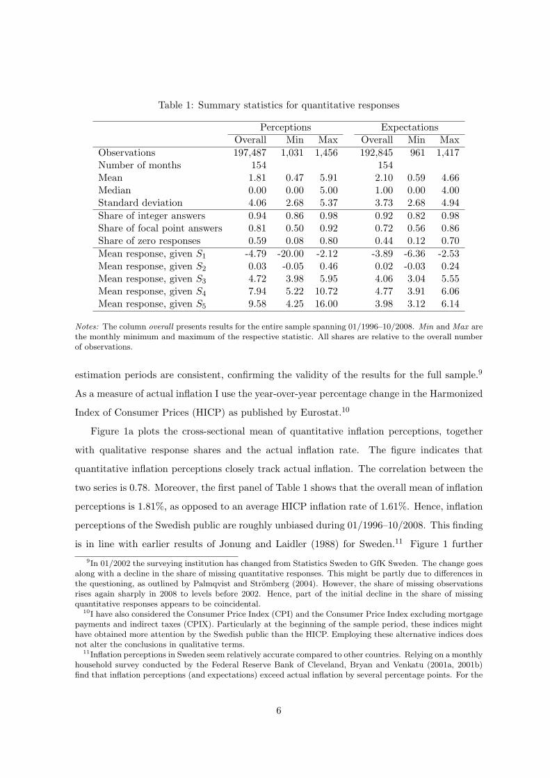
Table 1: Summary statistics for quantitative responses

Perceptions ExpectationsOverall Min Max Overall Min Max

Observations 197,487 1,031 1,456 192,845 961 1,417Number of months 154 154Mean 1.81 0.47 5.91 2.10 0.59 4.66Median 0.00 0.00 5.00 1.00 0.00 4.00Standard deviation 4.06 2.68 5.37 3.73 2.68 4.94

Share of integer answers 0.94 0.86 0.98 0.92 0.82 0.98Share of focal point answers 0.81 0.50 0.92 0.72 0.56 0.86Share of zero responses 0.59 0.08 0.80 0.44 0.12 0.70

Mean response, given S1 -4.79 -20.00 -2.12 -3.89 -6.36 -2.53Mean response, given S2 0.03 -0.05 0.46 0.02 -0.03 0.24Mean response, given S3 4.72 3.98 5.95 4.06 3.04 5.55Mean response, given S4 7.94 5.22 10.72 4.77 3.91 6.06Mean response, given S5 9.58 4.25 16.00 3.98 3.12 6.14

Notes: The column overall presents results for the entire sample spanning 01/1996–10/2008. Min and Max arethe monthly minimum and maximum of the respective statistic. All shares are relative to the overall numberof observations.

estimation periods are consistent, confirming the validity of the results for the full sample.9

As a measure of actual inflation I use the year-over-year percentage change in the Harmonized

Index of Consumer Prices (HICP) as published by Eurostat.10

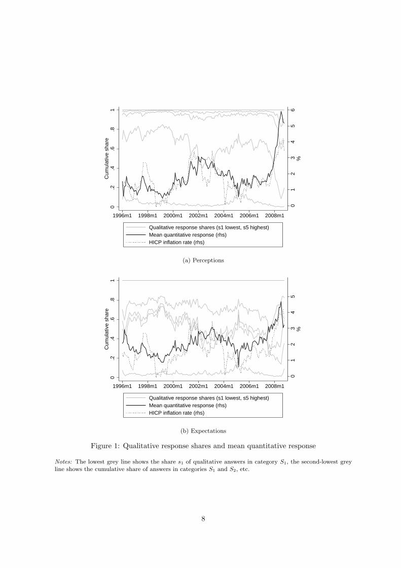
Figure 1a plots the cross-sectional mean of quantitative inflation perceptions, together

with qualitative response shares and the actual inflation rate. The figure indicates that

quantitative inflation perceptions closely track actual inflation. The correlation between the

two series is 0.78. Moreover, the first panel of Table 1 shows that the overall mean of inflation

perceptions is 1.81%, as opposed to an average HICP inflation rate of 1.61%. Hence, inflation

perceptions of the Swedish public are roughly unbiased during 01/1996–10/2008. This finding

is in line with earlier results of Jonung and Laidler (1988) for Sweden.11 Figure 1 further

9In 01/2002 the surveying institution has changed from Statistics Sweden to GfK Sweden. The change goesalong with a decline in the share of missing quantitative responses. This might be partly due to differences inthe questioning, as outlined by Palmqvist and Stromberg (2004). However, the share of missing observationsrises again sharply in 2008 to levels before 2002. Hence, part of the initial decline in the share of missingquantitative responses appears to be coincidental.

10I have also considered the Consumer Price Index (CPI) and the Consumer Price Index excluding mortgagepayments and indirect taxes (CPIX). Particularly at the beginning of the sample period, these indices mighthave obtained more attention by the Swedish public than the HICP. Employing these alternative indices doesnot alter the conclusions in qualitative terms.

11Inflation perceptions in Sweden seem relatively accurate compared to other countries. Relying on a monthlyhousehold survey conducted by the Federal Reserve Bank of Cleveland, Bryan and Venkatu (2001a, 2001b)find that inflation perceptions (and expectations) exceed actual inflation by several percentage points. For the

6

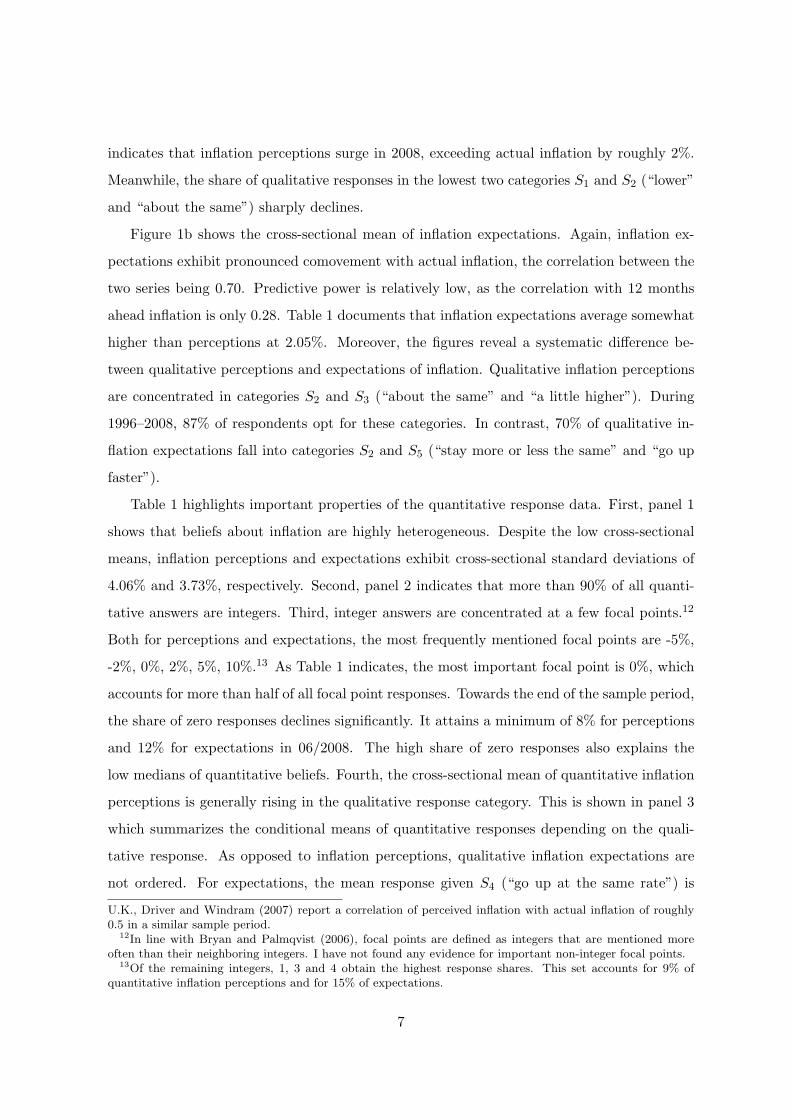
indicates that inflation perceptions surge in 2008, exceeding actual inflation by roughly 2%.

Meanwhile, the share of qualitative responses in the lowest two categories S1 and S2 (“lower”

and “about the same”) sharply declines.

Figure 1b shows the cross-sectional mean of inflation expectations. Again, inflation ex-

pectations exhibit pronounced comovement with actual inflation, the correlation between the

two series being 0.70. Predictive power is relatively low, as the correlation with 12 months

ahead inflation is only 0.28. Table 1 documents that inflation expectations average somewhat

higher than perceptions at 2.05%. Moreover, the figures reveal a systematic difference be-

tween qualitative perceptions and expectations of inflation. Qualitative inflation perceptions

are concentrated in categories S2 and S3 (“about the same” and “a little higher”). During

1996–2008, 87% of respondents opt for these categories. In contrast, 70% of qualitative in-

flation expectations fall into categories S2 and S5 (“stay more or less the same” and “go up

faster”).

Table 1 highlights important properties of the quantitative response data. First, panel 1

shows that beliefs about inflation are highly heterogeneous. Despite the low cross-sectional

means, inflation perceptions and expectations exhibit cross-sectional standard deviations of

4.06% and 3.73%, respectively. Second, panel 2 indicates that more than 90% of all quanti-

tative answers are integers. Third, integer answers are concentrated at a few focal points.12

Both for perceptions and expectations, the most frequently mentioned focal points are -5%,

-2%, 0%, 2%, 5%, 10%.13 As Table 1 indicates, the most important focal point is 0%, which

accounts for more than half of all focal point responses. Towards the end of the sample period,

the share of zero responses declines significantly. It attains a minimum of 8% for perceptions

and 12% for expectations in 06/2008. The high share of zero responses also explains the

low medians of quantitative beliefs. Fourth, the cross-sectional mean of quantitative inflation

perceptions is generally rising in the qualitative response category. This is shown in panel 3

which summarizes the conditional means of quantitative responses depending on the quali-

tative response. As opposed to inflation perceptions, qualitative inflation expectations are

not ordered. For expectations, the mean response given S4 (“go up at the same rate”) is

U.K., Driver and Windram (2007) report a correlation of perceived inflation with actual inflation of roughly0.5 in a similar sample period.

12In line with Bryan and Palmqvist (2006), focal points are defined as integers that are mentioned moreoften than their neighboring integers. I have not found any evidence for important non-integer focal points.

13Of the remaining integers, 1, 3 and 4 obtain the highest response shares. This set accounts for 9% ofquantitative inflation perceptions and for 15% of expectations.

7

01

23

45

6%

0.2

.4.6

.81

Cum

ulat

ive

shar

e

1996m1 1998m1 2000m1 2002m1 2004m1 2006m1 2008m1

Qualitative response shares (s1 lowest, s5 highest)Mean quantitative response (rhs)HICP inflation rate (rhs)

(a) Perceptions

01

23

45

%

0.2

.4.6

.81

Cum

ulat

ive

shar

e

1996m1 1998m1 2000m1 2002m1 2004m1 2006m1 2008m1

Qualitative response shares (s1 lowest, s5 highest)Mean quantitative response (rhs)HICP inflation rate (rhs)

(b) Expectations

Figure 1: Qualitative response shares and mean quantitative response

Notes: The lowest grey line shows the share s1 of qualitative answers in category S1, the second-lowest greyline shows the cumulative share of answers in categories S1 and S2, etc.

8

higher than the mean response given S5 (“go up faster”). Also, in comparison to inflation

perceptions, the differences between the cross-sectional means given qualitative responses S3,

S4 and S5 are only minor.14 Fifth, the relation between quantitative and qualitative responses

is time varying. The differences between overall, minimum and maximum conditional means

are considerable for most categories. The only exception is S2 (“about the same”): Given

this qualitative response, the mean quantitative response is always close to 0%.

These initial results suggest that the relation between quantitative and qualitative beliefs

about inflation is complex. The response scheme, i.e. the formal relation between quan-

titative and qualitative responses, appears to be time varying. Moreover, the conditional

mean of quantitative expectations is not monotonously rising in the order of the qualitative

response categories. While the 5-category probability method allows for a time varying re-

sponse scheme, it imposes a certain symmetry on the response scheme and requires ordered

qualitative data. Regarding the distributional assumptions, the mean and median values in-

dicate that quantitative beliefs are positively skewed and therefore not normally distributed.

The concentration of answers at focal points, in particular at 0%, raises additional doubt

whether any of the common parametric distributions adequately describes the quantitative

response data. The next section thus discusses in detail whether the assumptions of the

probability method are consistent with the data.

3 Validity of the Probability Method

3.1 Theoretical Assumptions

This section tests the main theoretical assumptions of the 5-category probability method for

quantifying qualitative response data. Building on contributions of Theil (1952) and Carlson

and Parkin (1975), the 5-category probability method has been proposed by Batchelor and

Orr (1988). To begin with, the method is briefly outlined.

Assume that previous to answering the consumer survey, respondent i forms a quantitative

belief πet,i about inflation over the upcoming 12 months.15 Respondent i then answers the

14On a monthly basis, the mean of inflation perceptions is not always strictly rising too. This is indicatedby the minima of monthly conditional means in panel 3 of Table 1. But the conditional means lack order onlyin 27 months, as opposed to 136 months for inflation expectations.

15The analogous approach for quantifying perceived inflation πpt,i and detailed derivations can be found in

Appendix A.1.

9

qualitative survey question on expected inflation according to the following response scheme:

πet,i < −δt : prices in general will go down a little (S1)

−δt ≤ πet,i < δt : stay more or less the same (S2)

δt ≤ πet,i < πr

t − ηt : go up more slowly (S3)

πrt − ηt ≤ πe

t,i < πrt + ηt : go up at the same rate (S4)

πet,i ≥ πr

t + ηt : go up faster (S5) (1)

The response scheme is defined by the parameters δt, ηt and πrt . In the following, πr

t is

referred to as reference inflation. It is the inflation rate that people have in mind when opting

for answer S4 (“prices will go up at the same rate” and, for inflation perceptions, “prices

are moderately higher”). The first key assumption of the probability method restricts the

response scheme to be fully defined by these three parameters:

Assumption 1: The response intervals are symmetric around 0% and around πrt .

The corresponding intervals [−δt, δt) and [πrt −ηt, π

rt +ηt) correspond to qualitative responses

S2 and S4 respectively. A second assumption imposes structural homogeneity on the response

scheme:

Assumption 2: Threshold parameters δt and ηt and the reference inflation πrt are identical

across respondents.

Quantitative inflation expectations πet,i will vary across respondents due to differences in

information sets and information processing. To infer the mean quantitative inflation ex-

pectation from qualitative response shares, the probability method imposes a distributional

assumption on πet,i. The standard assumption is that the cross-sectional distribution of quan-

titative beliefs is normal:

Assumption 3: The cross-sectional distribution of quantitative beliefs is normal, i.e. πet,i ∼

N(πet , (σ

et )

2).

The parameters of interest are the cross-sectional mean πet and standard deviation σe

t of

quantitative beliefs. As outlined in Appendix A.1, the above assumptions yield a system of

4 linearly independent equations with 5 unknowns (πet σe

t , δt, ηt, πrt ) which can be solved for

πet and σe

t . The solution for both parameters is equal to the product of reference inflation πrt

and a function of the response shares s1t , ..., s5t .

10

The usual identification scheme restricts reference inflation πrt . For quantifying inflation

expectations two choices of πrt are apparent. First, reference inflation can be set equal to

some actual rate of inflation, assuming that the respondent knows the actual rate of inflation

and answers the question relative to this value. Second, reference inflation can be set equal

to previously quantified perceived inflation πpt as suggested by Berk (1999). This approach

is supported by empirical evidence that households are not necessarily well informed about

actual inflation.16 Identifying πrt is less obvious for inflation perceptions. Following Carlson

and Parkin (1975) it is commonly assumed that inflation perceptions are unbiased over the

sample horizon. This assumption can be imposed by restricting πrt to a constant accordingly.

17

The last assumption thus reads:

Assumption 4: The reference rate of inflation πrt for quantifying inflation expectations is

equal to actual inflation or quantified perceived inflation. The reference rate of inflation

for quantifying inflation perceptions is time invariant.

3.2 Symmetry of the Response Scheme

Assumption 1 restricts response intervals to be symmetric around 0% and around πrt . To

test the validity of this assumption I estimate an unrestricted response scheme defined by 4

threshold parameters. Assume that respondent i answers the qualitative question according

to the following scheme:18

πet,i + εt,i < µ1

t : prices in general will go down a little (S1)

µ1t ≤ πe

t,i + εt,i < µ2t : stay more or less the same (S2)

µ2t ≤ πe

t,i + εt,i < µ3t : go up more slowly (S3)

µ3t ≤ πe

t,i + εt,i < µ4t : go up at the same rate (S4)

πet,i + εt,i ≥ µ4

t : go up faster (S5) (2)

The idiosyncratic component εt,i allows the response scheme to shift between individuals.

Under the assumption that the idiosyncratic component represents the sum of independent

idiosyncratic factors it is reasonable to assume that εt,i is normally distributed. One thus

16See, e.g., Bryan and Venkatu (2001a, 2001b) who document that inflation perceptions of U.S. householdsare significantly biased.

17The solution for πrt is given by Equation (A.7) in the Appendix.

18The identical scheme applies to inflation perceptions, with πet,i being replaced by πp

t,i.

11

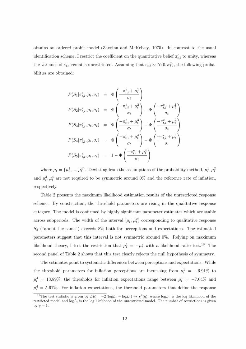
obtains an ordered probit model (Zavoina and McKelvey, 1975). In contrast to the usual

identification scheme, I restrict the coefficient on the quantitative belief πet,i to unity, whereas

the variance of εt,i remains unrestricted. Assuming that εt,i ∼ N(0, σ2t ), the following proba-

bilities are obtained:

P (S1|πet,i, µt, σt) = Φ

(−πe

t,i + µ1t

σt

)

P (S2|πet,i, µt, σt) = Φ

(−πe

t,i + µ2t

σt

)− Φ

(−πe

t,i + µ1t

σt

)

P (S3|πet,i, µt, σt) = Φ

(−πe

t,i + µ3t

σt

)− Φ

(−πe

t,i + µ2t

σt

)

P (S4|πet,i, µt, σt) = Φ

(−πe

t,i + µ4t

σt

)− Φ

(−πe

t,i + µ3t

σt

)

P (S5|πet,i, µt, σt) = 1− Φ

(−πe

t,i + µ4t

σt

)

where µt = {µ1t , ..., µ

4t }. Deviating from the assumptions of the probability method, µ1

t , µ2t

and µ3t , µ

4t are not required to be symmetric around 0% and the reference rate of inflation,

respectively.

Table 2 presents the maximum likelihood estimation results of the unrestricted response

scheme. By construction, the threshold parameters are rising in the qualitative response

category. The model is confirmed by highly significant parameter estimates which are stable

across subperiods. The width of the interval [µ1t , µ

2t ) corresponding to qualitative response

S2 (“about the same”) exceeds 8% both for perceptions and expectations. The estimated

parameters suggest that this interval is not symmetric around 0%. Relying on maximum

likelihood theory, I test the restriction that µ1t = −µ2

t with a likelihood ratio test.19 The

second panel of Table 2 shows that this test clearly rejects the null hypothesis of symmetry.

The estimates point to systematic differences between perceptions and expectations. While

the threshold parameters for inflation perceptions are increasing from µ1t = −6.91% to

µ4t = 13.89%, the thresholds for inflation expectations range between µ1

t = −7.04% and

µ4t = 5.61%. For inflation expectations, the threshold parameters that define the response

19The test statistic is given by LR = −2 (logLr − logLi) → χ2(q), where logLr is the log likelihood of therestricted model and logLi is the log likelihood of the unrestricted model. The number of restrictions is givenby q = 1.

12

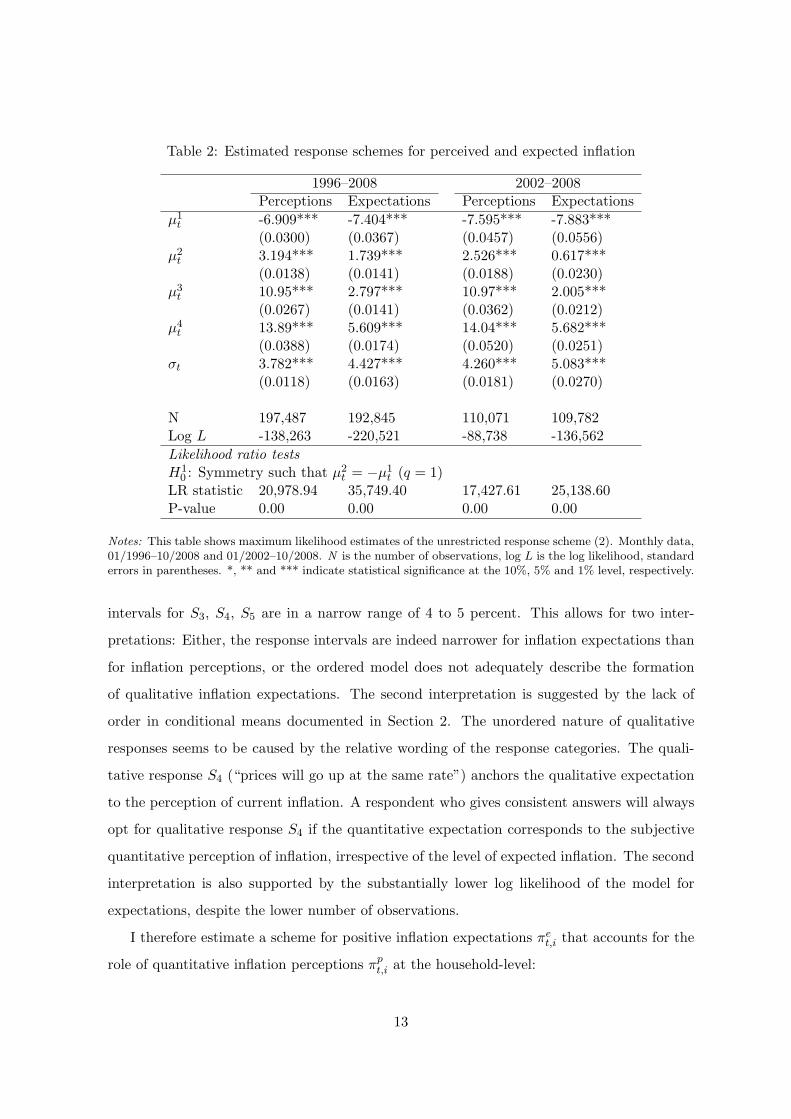
Table 2: Estimated response schemes for perceived and expected inflation

1996–2008 2002–2008Perceptions Expectations Perceptions Expectations

µ1t -6.909*** -7.404*** -7.595*** -7.883***

(0.0300) (0.0367) (0.0457) (0.0556)µ2t 3.194*** 1.739*** 2.526*** 0.617***

(0.0138) (0.0141) (0.0188) (0.0230)µ3t 10.95*** 2.797*** 10.97*** 2.005***

(0.0267) (0.0141) (0.0362) (0.0212)µ4t 13.89*** 5.609*** 14.04*** 5.682***

(0.0388) (0.0174) (0.0520) (0.0251)σt 3.782*** 4.427*** 4.260*** 5.083***

(0.0118) (0.0163) (0.0181) (0.0270)

N 197,487 192,845 110,071 109,782Log L -138,263 -220,521 -88,738 -136,562

Likelihood ratio testsH1

0 : Symmetry such that µ2t = −µ1

t (q = 1)LR statistic 20,978.94 35,749.40 17,427.61 25,138.60P-value 0.00 0.00 0.00 0.00

Notes: This table shows maximum likelihood estimates of the unrestricted response scheme (2). Monthly data,01/1996–10/2008 and 01/2002–10/2008. N is the number of observations, log L is the log likelihood, standarderrors in parentheses. *, ** and *** indicate statistical significance at the 10%, 5% and 1% level, respectively.

intervals for S3, S4, S5 are in a narrow range of 4 to 5 percent. This allows for two inter-

pretations: Either, the response intervals are indeed narrower for inflation expectations than

for inflation perceptions, or the ordered model does not adequately describe the formation

of qualitative inflation expectations. The second interpretation is suggested by the lack of

order in conditional means documented in Section 2. The unordered nature of qualitative

responses seems to be caused by the relative wording of the response categories. The quali-

tative response S4 (“prices will go up at the same rate”) anchors the qualitative expectation

to the perception of current inflation. A respondent who gives consistent answers will always

opt for qualitative response S4 if the quantitative expectation corresponds to the subjective

quantitative perception of inflation, irrespective of the level of expected inflation. The second

interpretation is also supported by the substantially lower log likelihood of the model for

expectations, despite the lower number of observations.

I therefore estimate a scheme for positive inflation expectations πet,i that accounts for the

role of quantitative inflation perceptions πpt,i at the household-level:

13

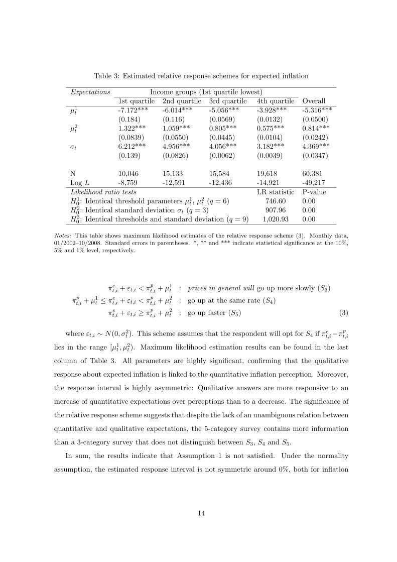
Table 3: Estimated relative response schemes for expected inflation

Expectations Income groups (1st quartile lowest)1st quartile 2nd quartile 3rd quartile 4th quartile Overall

µ1t -7.172*** -6.014*** -5.056*** -3.928*** -5.316***

(0.184) (0.116) (0.0569) (0.0132) (0.0500)µ2t 1.322*** 1.059*** 0.805*** 0.575*** 0.814***

(0.0839) (0.0550) (0.0445) (0.0104) (0.0242)σt 6.212*** 4.956*** 4.056*** 3.182*** 4.369***

(0.139) (0.0826) (0.0062) (0.0039) (0.0347)

N 10,046 15,133 15,584 19,618 60,381Log L -8,759 -12,591 -12,436 -14,921 -49,217

Likelihood ratio tests LR statistic P-valueH1

0 : Identical threshold parameters µ1t , µ

2t (q = 6) 746.60 0.00

H20 : Identical standard deviation σt (q = 3) 907.96 0.00

H30 : Identical thresholds and standard deviation (q = 9) 1,020.93 0.00

Notes: This table shows maximum likelihood estimates of the relative response scheme (3). Monthly data,01/2002–10/2008. Standard errors in parentheses. *, ** and *** indicate statistical significance at the 10%,5% and 1% level, respectively.

πet,i + εt,i < πp

t,i + µ1t : prices in general will go up more slowly (S3)

πpt,i + µ1

t ≤ πet,i + εt,i < πp

t,i + µ2t : go up at the same rate (S4)

πet,i + εt,i ≥ πp

t,i + µ2t : go up faster (S5) (3)

where εt,i ∼ N(0, σ2t ). This scheme assumes that the respondent will opt for S4 if π

et,i−πp

t,i

lies in the range [µ1t , µ

2t ). Maximum likelihood estimation results can be found in the last

column of Table 3. All parameters are highly significant, confirming that the qualitative

response about expected inflation is linked to the quantitative inflation perception. Moreover,

the response interval is highly asymmetric: Qualitative answers are more responsive to an

increase of quantitative expectations over perceptions than to a decrease. The significance of

the relative response scheme suggests that despite the lack of an unambiguous relation between

quantitative and qualitative expectations, the 5-category survey contains more information

than a 3-category survey that does not distinguish between S3, S4 and S5.

In sum, the results indicate that Assumption 1 is not satisfied. Under the normality

assumption, the estimated response interval is not symmetric around 0%, both for inflation

14

perceptions and expectations.20 Furthermore, the response interval is not symmetric around

πrt for inflation expectations. The estimations confirm that qualitative inflation expectations

are formed relative to perceived inflation. This result suggests that the link between expec-

tations and perceptions should be exploited in quantifying qualitative responses.

3.3 Homogeneity of the Response Scheme

Assumption 2 imposes that threshold parameters δt and ηt and reference inflation πrt are ho-

mogeneous across respondents. Since the Swedish dataset only contains one observation per

individual, this assumption is tested by estimating the response scheme for different income

groups.21 Tables 4 and 5 summarize the estimation results for perceptions and expectations,

respectively. The tables show that the absolute values of threshold parameters tend to decline

in income. The lower panel of Tables 4 and 5 show likelihood ratio tests of three restrictions.

The null hypotheses state that threshold parameters are identical across income groups (H10 ),

that standard deviations are identical across income groups (H20 ) and that threshold param-

eters and standard deviations are identical across income groups (H30 ). All three hypotheses

are clearly rejected.

Table 3 presents estimation results for the relative response scheme (3) that links expected

inflation to perceived inflation. Again, all three hypotheses are clearly rejected. The estimates

show the same pattern as above: The absolute values of threshold parameters are declining in

income. Overall, these results suggest that the response scheme systematically differs across

income-groups, which implies that Assumption 2 is violated.22

20This finding is consistent with Henzel and Wollmershauser (2005) who investigate data from a specialedition of the ifo World Economic Survey that directly asks respondents to indicate the indifference interval.Henzel and Wollmershauser (2005) report that the positive threshold parameter is larger in absolute termsthan the negative parameter. As opposed to the Swedish survey, however, the ifo survey queries professionalforecasters and answers are given on a 3-category ordinal scale.

21I have also considered educational groups, with unchanged qualitative results.22Note that the mean of beliefs about inflation also depends on socioeconomic characteristics. The cross-

sectional means of perceptions and expectations are declining in income. This pattern is consistent with theestimated response schemes that suggest that individuals in the highest income quartile experience deviationsof inflation from zero as more relevant in qualitative terms than individuals in lower income quartiles.

15

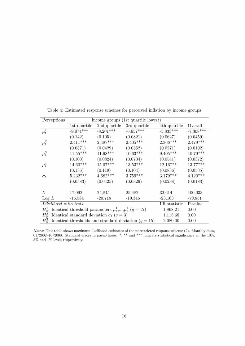
Table 4: Estimated response schemes for perceived inflation by income groups

Perceptions Income groups (1st quartile lowest)1st quartile 2nd quartile 3rd quartile 4th quartile Overall

µ1t -9.074*** -8.201*** -6.657*** -5.833*** -7.308***

(0.142) (0.105) (0.0821) (0.0627) (0.0459)µ2t 2.411*** 2.487*** 2.405*** 2.366*** 2.479***

(0.0571) (0.0429) (0.0352) (0.0271) (0.0192)µ3t 11.55*** 11.68*** 10.63*** 9.405*** 10.79***

(0.100) (0.0824) (0.0704) (0.0541) (0.0372)µ4t 14.60*** 15.07*** 13.53*** 12.16*** 13.77***

(0.136) (0.119) (0.104) (0.0836) (0.0535)σt 5.232*** 4.682*** 3.759*** 3.179*** 4.120***

(0.0583) (0.0425) (0.0326) (0.0238) (0.0183)

N 17,092 24,845 25,482 32,614 100,033Log L -15,584 -20,718 -19,346 -23,163 -79,851

Likelihood ratio tests LR statistic P-valueH1

0 : Identical threshold parameters µ1t ,...,µ

4t (q = 12) 1,868.21 0.00

H20 : Identical standard deviation σt (q = 3) 1,115.68 0.00

H30 : Identical thresholds and standard deviation (q = 15) 2,080.00 0.00

Notes: This table shows maximum likelihood estimates of the unrestricted response scheme (2). Monthly data,01/2002–10/2008. Standard errors in parentheses. *, ** and *** indicate statistical significance at the 10%,5% and 1% level, respectively.

16

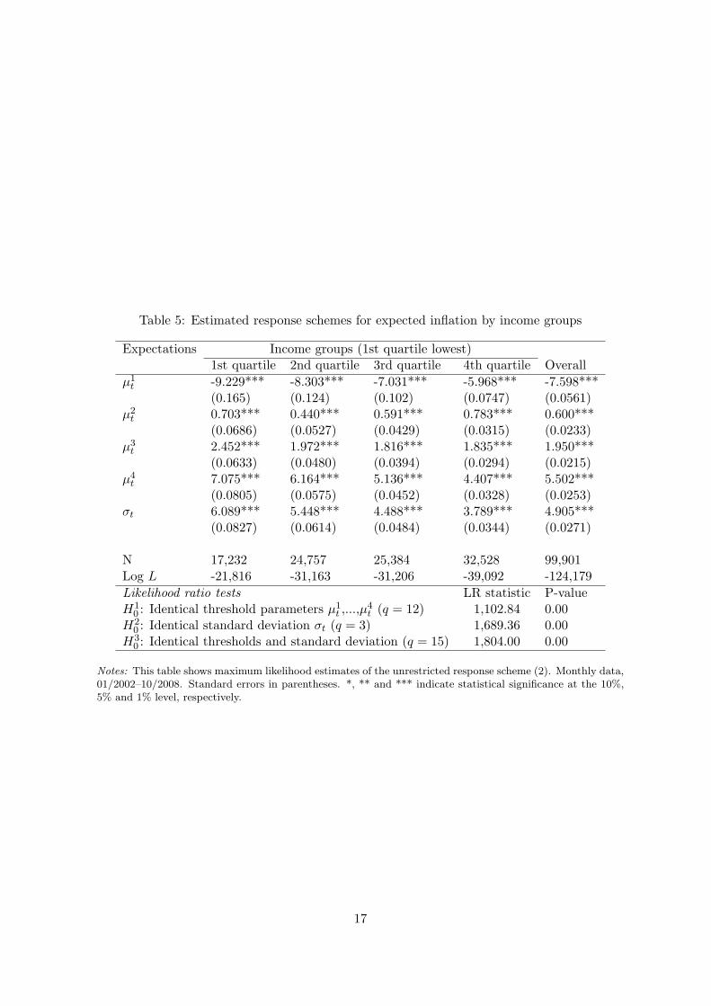
Table 5: Estimated response schemes for expected inflation by income groups

Expectations Income groups (1st quartile lowest)1st quartile 2nd quartile 3rd quartile 4th quartile Overall

µ1t -9.229*** -8.303*** -7.031*** -5.968*** -7.598***

(0.165) (0.124) (0.102) (0.0747) (0.0561)µ2t 0.703*** 0.440*** 0.591*** 0.783*** 0.600***

(0.0686) (0.0527) (0.0429) (0.0315) (0.0233)µ3t 2.452*** 1.972*** 1.816*** 1.835*** 1.950***

(0.0633) (0.0480) (0.0394) (0.0294) (0.0215)µ4t 7.075*** 6.164*** 5.136*** 4.407*** 5.502***

(0.0805) (0.0575) (0.0452) (0.0328) (0.0253)σt 6.089*** 5.448*** 4.488*** 3.789*** 4.905***

(0.0827) (0.0614) (0.0484) (0.0344) (0.0271)

N 17,232 24,757 25,384 32,528 99,901Log L -21,816 -31,163 -31,206 -39,092 -124,179

Likelihood ratio tests LR statistic P-valueH1

0 : Identical threshold parameters µ1t ,...,µ

4t (q = 12) 1,102.84 0.00

H20 : Identical standard deviation σt (q = 3) 1,689.36 0.00

H30 : Identical thresholds and standard deviation (q = 15) 1,804.00 0.00

Notes: This table shows maximum likelihood estimates of the unrestricted response scheme (2). Monthly data,01/2002–10/2008. Standard errors in parentheses. *, ** and *** indicate statistical significance at the 10%,5% and 1% level, respectively.

17

3.4 Normality of Quantitative Responses

Assumption 3 requires that the cross-sectional distribution of quantitative beliefs is normal.

Normality has been tested and rejected for inflation expectations of consumers (Batchelor and

Dua, 1987) and professional forecasters (Carlson, 1975, Lahiri and Teigland, 1987). These

studies generally find that quantitative beliefs are positively skewed and leptokurtic. Both

patterns can also be found in the Swedish survey data, as panel 1 of Table 6 indicates. Beliefs

about inflation exhibit a pronounced positive skewness and are leptokurtic. Consequently,

the Jarque-Bera test rejects the null hypothesis of normality in every single survey month, as

panel 2 of Table 6 shows.

More generally, the probability method requires that beliefs follow some identifiable para-

metric distribution. Lahiri and Teigland (1987) suggest a noncentral t distribution as an

alternative to the normal distribution. The noncentral t distribution allows for positive skew-

ness and fat tails. I formally test whether quantitative responses follow this distribution using

the Kolmogorov-Smirnov test.23 Results are summarized in panel 3 of Table 6 and show that

this null hypothesis is also rejected in all months.

These formal tests do not answer the question which parametric distribution produces

the best quantification results. The answer will also depend on the time period. During

1996–2007, the high share of zero responses cannot be reconciled with both the normal and

noncentral t distributions. With the rise in perceptions and expectations of inflation in 2008,

the shape of the empirical distribution becomes somewhat smoother and less skewed, as the

share of zero responses declines. Overall, the results indicate that differences in the relative

fit of common parametric distributions are predominated by the high share of zero responses.

This conjecture is consistent with Berk (1999), Dasgupta and Lahiri (1992) and Smith and

McAleer (1995) who find that the accuracy of the quantified series does not significantly vary

between any of the common parametric distributions.

23The Kolmogorov-Smirnov statistic is given by Dn(F ) = supx |Fn(x)− F (x)|, where Fn(.) is the empiricaldistribution function. Note that the noncentral t distribution is equal to the t distribution if the noncentralityparameter µ is zero.

18

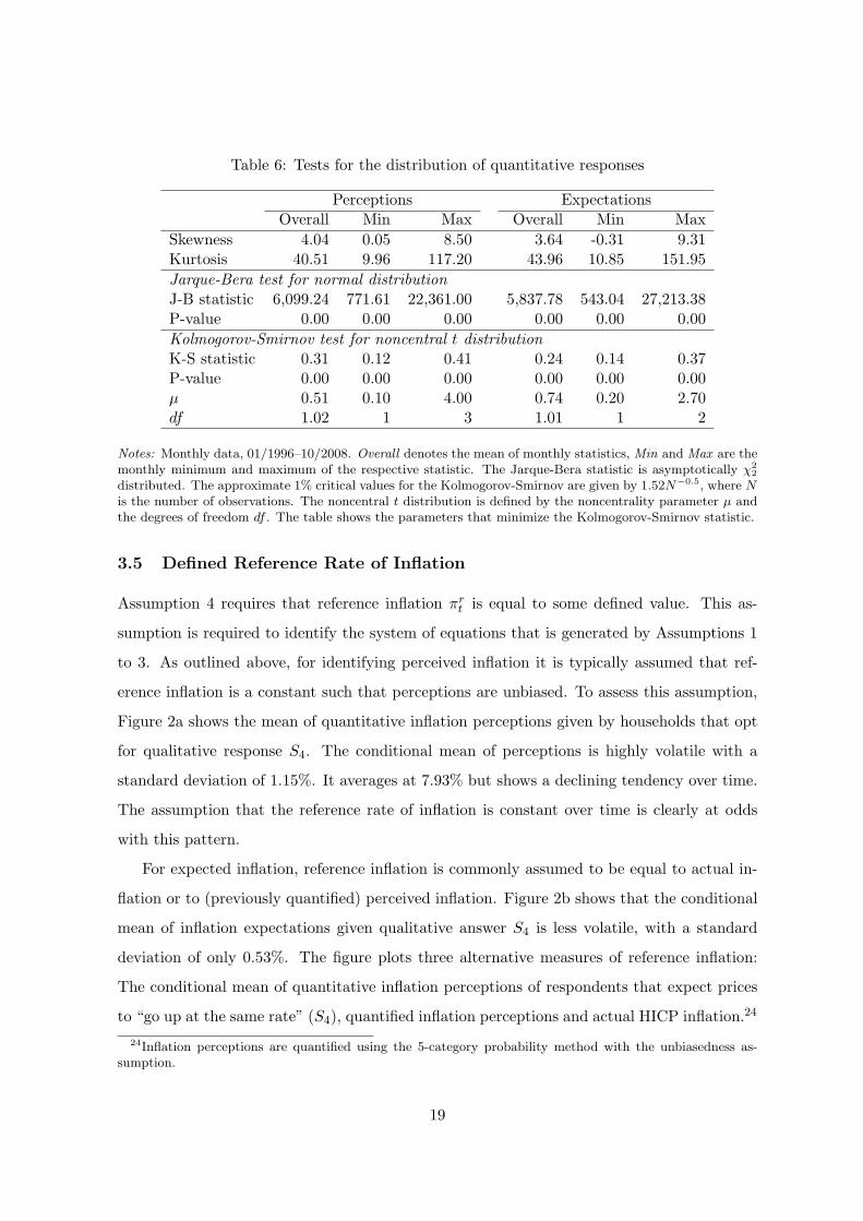
Table 6: Tests for the distribution of quantitative responses

Perceptions ExpectationsOverall Min Max Overall Min Max

Skewness 4.04 0.05 8.50 3.64 -0.31 9.31Kurtosis 40.51 9.96 117.20 43.96 10.85 151.95

Jarque-Bera test for normal distributionJ-B statistic 6,099.24 771.61 22,361.00 5,837.78 543.04 27,213.38P-value 0.00 0.00 0.00 0.00 0.00 0.00

Kolmogorov-Smirnov test for noncentral t distributionK-S statistic 0.31 0.12 0.41 0.24 0.14 0.37P-value 0.00 0.00 0.00 0.00 0.00 0.00µ 0.51 0.10 4.00 0.74 0.20 2.70df 1.02 1 3 1.01 1 2

Notes: Monthly data, 01/1996–10/2008. Overall denotes the mean of monthly statistics, Min and Max are themonthly minimum and maximum of the respective statistic. The Jarque-Bera statistic is asymptotically χ2

2

distributed. The approximate 1% critical values for the Kolmogorov-Smirnov are given by 1.52N−0.5, where Nis the number of observations. The noncentral t distribution is defined by the noncentrality parameter µ andthe degrees of freedom df . The table shows the parameters that minimize the Kolmogorov-Smirnov statistic.

3.5 Defined Reference Rate of Inflation

Assumption 4 requires that reference inflation πrt is equal to some defined value. This as-

sumption is required to identify the system of equations that is generated by Assumptions 1

to 3. As outlined above, for identifying perceived inflation it is typically assumed that ref-

erence inflation is a constant such that perceptions are unbiased. To assess this assumption,

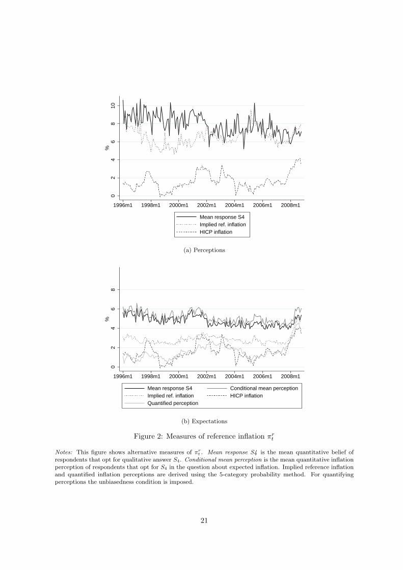
Figure 2a shows the mean of quantitative inflation perceptions given by households that opt

for qualitative response S4. The conditional mean of perceptions is highly volatile with a

standard deviation of 1.15%. It averages at 7.93% but shows a declining tendency over time.

The assumption that the reference rate of inflation is constant over time is clearly at odds

with this pattern.

For expected inflation, reference inflation is commonly assumed to be equal to actual in-

flation or to (previously quantified) perceived inflation. Figure 2b shows that the conditional

mean of inflation expectations given qualitative answer S4 is less volatile, with a standard

deviation of only 0.53%. The figure plots three alternative measures of reference inflation:

The conditional mean of quantitative inflation perceptions of respondents that expect prices

to “go up at the same rate” (S4), quantified inflation perceptions and actual HICP inflation.24

24Inflation perceptions are quantified using the 5-category probability method with the unbiasedness as-sumption.

19

Clearly, the conditional mean of inflation perceptions closely follows the conditional mean of

inflation expectations. The correlation coefficient of the two series is 0.94, the average level

difference only 0.39%. The similarity of these series is in line with the finding that qualitative

expectations are formed relative to quantitative perceptions. In contrast, the correlations

of the conditional mean with quantified inflation perceptions and actual inflation are -0.15

and 0.06, respectively. In both cases, the level difference is substantial. Consequently, the as-

sumption that reference inflation corresponds to quantified or actual inflation can be rejected.

However, the correlations of the conditional mean with quantified inflation perceptions and

actual inflation increase to 0.46 and 0.41 during 2002–2008. Notably, a comovement of these

measures of moderate inflation with the conditional mean is apparent towards the end of the

sample period, when actual inflation substantially increases.

Alternatively, Assumption 4 can be assessed based on the implied level of reference in-

flation. The implied level of reference inflation is obtained by combining the cross-sectional

mean of quantitative responses with Assumptions 1 to 3.25 Assessing this series amounts

to a joint test of Assumptions 1 to 3. Figure 2a indicates that implied reference inflation

fluctuates around a similar level as the conditional mean of inflation perceptions. However,

the correlation between the two series is 0.06. For inflation expectations shown in Figure 2b,

the implied reference inflation averages 2% below the conditional mean. The correlation of

the two series is 0.31. Provided that the true reference rate of inflation is equal to the condi-

tional mean given qualitative answer S4, these results suggests that Assumptions 1 to 3 can

be jointly rejected. In light of this finding, the next section assesses the joint validity of all 4

hypotheses in more detail.

3.6 Joint Assessment

While all four hypotheses can be individually rejected, this section investigates the joint

validity of the assumptions. The focus does not lie on rejection/non-rejection but rather on

the degree of overall validity. I proceed by quantifying the qualitative survey data with the

5-category probability method.26 This yields the threshold parameters δt and ηt which can

25Given the cross-sectional mean πet of quantitative inflation expectations, implied reference inflation can be

obtained by rearranging Equation (A.3).26Inflation perceptions are quantified by imposing the unbiasedness condition. For inflation expectations it is

assumed that reference inflation is equal to quantified inflation perceptions. Detailed derivations are providedin Appendix A.1.

20

02

46

810

%

1996m1 1998m1 2000m1 2002m1 2004m1 2006m1 2008m1

Mean response S4Implied ref. inflationHICP inflation

(a) Perceptions

02

46

8%

1996m1 1998m1 2000m1 2002m1 2004m1 2006m1 2008m1

Mean response S4 Conditional mean perceptionImplied ref. inflation HICP inflationQuantified perception

(b) Expectations

Figure 2: Measures of reference inflation πrt

Notes: This figure shows alternative measures of πrt . Mean response S4 is the mean quantitative belief of

respondents that opt for qualitative answer S4. Conditional mean perception is the mean quantitative inflationperception of respondents that opt for S4 in the question about expected inflation. Implied reference inflationand quantified inflation perceptions are derived using the 5-category probability method. For quantifyingperceptions the unbiasedness condition is imposed.

21

be used to construct the implied response scheme on a monthly basis.

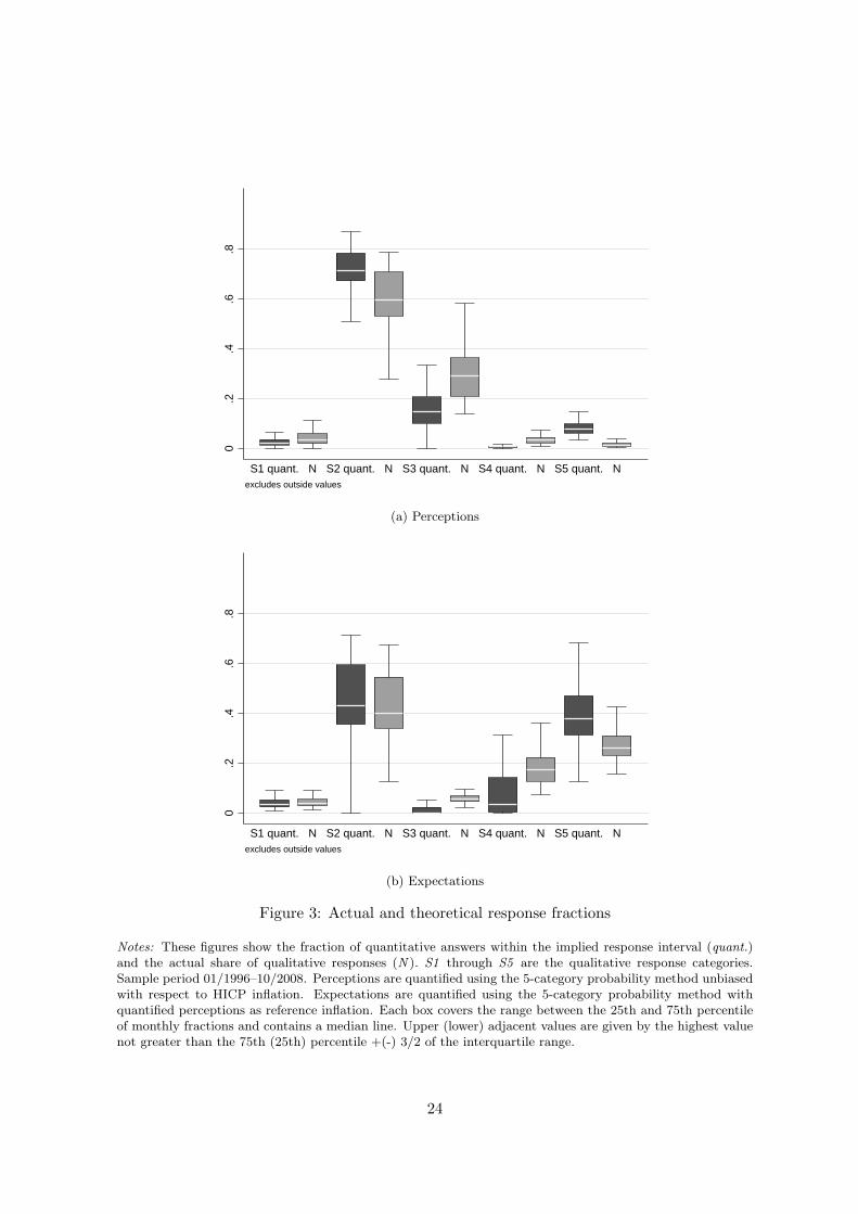
Figure 3 shows box plots of the distribution of monthly response shares. For each answer

category, the fraction of quantitative beliefs that lie within the implied response interval

(“quant.”) is compared to the actual share of qualitative responses (“N”).27 For inflation

perceptions, Figure 3a signals pronounced deviations of implied from actual response fractions

in categories S3 and S5. The high share of quantitative responses in the implied range of S5

is consistent with the previous finding that the distribution of responses is positively skewed

and leptokurtic. Moreover, the low fraction of quantitative responses in the implied range of

S3 appears to be a direct consequence of fitting the normal distribution to the high share of

zero responses.

A similar pattern is obtained for inflation expectations. Figure 3b illustrates that the

deviation of the implied from the actual response share is highest for categories S3, S4 and

S5. Similar to perceptions, the fraction of quantitative responses in the implied range of S5

exceeds the actual share of qualitative responses. This pattern also relates to the finding of

the previous section, according to which the mean quantitative answer of respondents opting

for qualitative answer S4 is significantly higher than actual inflation or quantified inflation

perceptions. Consequently, a large fraction of these quantitative answers fall into the interval

of the qualitative answer S5.

Further insights can be gained by looking at the fraction of quantitative responses that lie

below or above the implied response interval. Figure A.1 in the Appendix shows these fractions

relative to the number of responses in the respective qualitative response category. Both for

perceptions and expectations, the figure reveals that the 5-category probability method best

accommodates qualitative answer S2. On average, 99% of quantitative responses associated

with qualitative answer S2 lie within the implied response interval. S2 is the most important

qualitative response, accounting for roughly 59% of perceptions and 42% of expectations

during 1996–2008. Regarding inflation perceptions shown in Figure A.1a, coverage for the

second most important category S3, which obtains 30% of responses, is lower. Only about

30% of quantitative responses are within the implied response interval. A relatively large

share of quantitative responses lies below the implied response interval, indicating that the

interval around 0% is too wide. The worst coverage results for S4, but only 4% of respondents

27Note that by construction, the actual share of qualitative responses corresponds to the predicted share ofquantitative responses under the normality assumption.

22

opt for this qualitative category.

The pattern is different for inflation expectations. Figure A.1b indicates that only about

10% of quantitative beliefs fall into the implied response intervals for S3 and S4. Most

quantitative responses are above the implied interval. This can be explained by the high

share of on average 27% of responses in category S5. Fitting this share leads to a downward

shift of the lower response intervals. Moreover, the previous section has shown that quantified

perceptions are significantly lower than reference inflation πr. Hence, the implied response

intervals linked to quantified perceptions will be too low.

The above findings also hold in the 01/2002–10/2008 subperiod, as Figures A.2 and A.3 in

the Appendix confirm. In sum, the results suggest that Assumptions 1 through 4 are invalid.

This leads to significant distortions primarily concerning the incorporation of information

from positive categories S3, S4, S5, which seem more pronounced for inflation expectations

than for inflation perceptions. The next section assesses the implications for the accuracy of

the probability method.

23

0.2

.4.6

.8

S1 quant. N S2 quant. N S3 quant. N S4 quant. N S5 quant. Nexcludes outside values

(a) Perceptions

0.2

.4.6

.8

S1 quant. N S2 quant. N S3 quant. N S4 quant. N S5 quant. Nexcludes outside values

(b) Expectations

Figure 3: Actual and theoretical response fractions

Notes: These figures show the fraction of quantitative answers within the implied response interval (quant.)and the actual share of qualitative responses (N ). S1 through S5 are the qualitative response categories.Sample period 01/1996–10/2008. Perceptions are quantified using the 5-category probability method unbiasedwith respect to HICP inflation. Expectations are quantified using the 5-category probability method withquantified perceptions as reference inflation. Each box covers the range between the 25th and 75th percentileof monthly fractions and contains a median line. Upper (lower) adjacent values are given by the highest valuenot greater than the 75th (25th) percentile +(-) 3/2 of the interquartile range.

24

4 Accuracy of the Probability Method

4.1 Level and Dynamics of Beliefs

This section assesses the accuracy of the 5-category probability method relative to the mean of

actual quantitative survey responses. Perceptions and expectations of inflation are quantified

by imposing the usual restrictions. Inflation perceptions are assumed to be unbiased with

respect to HICP inflation. Inflation expectations are quantified by setting reference infla-

tion equal to HICP inflation and alternatively, following Berk (1999), to quantified perceived

inflation.28 The 5-category probability method is compared to a set of alternative quantifi-

cation methods. The first alternative is the 3-category probability method of Carlson and

Parkin (1975).29 The second alternative is the scaled balance statistic with mean and vari-

ance of actual inflation. In line with the literature, the 5-category balance statistic is given by

s5+0.5s4−0.5s2−s1. The 3-category balance statistic is given by s5+s4+s3−s1 = spt −snt ,

where spt and snt are the fractions of respondents that report that prices are rising and falling,

respectively. The third alternative is the Pesaran (1987) regression approach for 3-category

response data.30

The primary measure of accuracy I consider is the (Pearson) correlation coefficient between

the quantified series and the cross-sectional mean of quantitative responses. As opposed to the

mean absolute error (MAE) or root mean squared error (RMSE), the correlation coefficient

is robust to a constant scaling of the involved series. In particular, the correlation coefficient

is unaffected by the average level of reference inflation πr. Another advantage of employing

the correlation coefficient is that its distributional properties have been explored. The Fisher

z-transformation of the correlation coefficient results in an approximately normal random

variable, provided the underlying data follows a bivariate normal distribution. Relying on

the Fisher z-transformation, the null hypothesis that two correlation coefficients are equal

28Perceived inflation is quantified using the 5-category probability method under the assumption of unbi-asedness with respect to HICP inflation.

29Answer categories are aggregated following Berk (1999), see Appendix A.2 for details.30Unlike the early regression approaches suggested by Theil (1952) and Anderson (1952), the Pesaran (1987)

approach allows for asymmetric response behavior in periods of rising and falling inflation. The Pesaran

approach is based on nonlinear least squares estimation of the model πt =β1s

pt −β2s

nt

1−β3spt

+ εt, where πt denotes

actual HICP inflation. Expected inflation is generated in a second step as a prediction of this model basedon answering fractions about inflation expectations (where coefficient estimates are obtained in the first stepusing perceptions data). A measure of perceived inflation is computed as the prediction of the model usingthe perceptions data it has been estimated with.

25

(ρ1 = ρ2) can be tested using the following statistic:

z = tanh−1(ρ1)− tanh−1(ρ2) (4)

where tanh−1(ρi) = 0.5ln(1+ρi1−ρi

). The z statistic is approximately normal with variance

1T1−3 + 1

T2−3 , where T1 and T2 are the sample sizes underlying correlation coefficients ρ1 and

ρ2, respectively. However, the normal approximation may be inaccurate in the present case

because |ρi| is high and the underlying series are serially dependent (Mudholkar, 2006). I

therefore assess significance based on double block bootstrap confidence intervals for the z

statistic.31

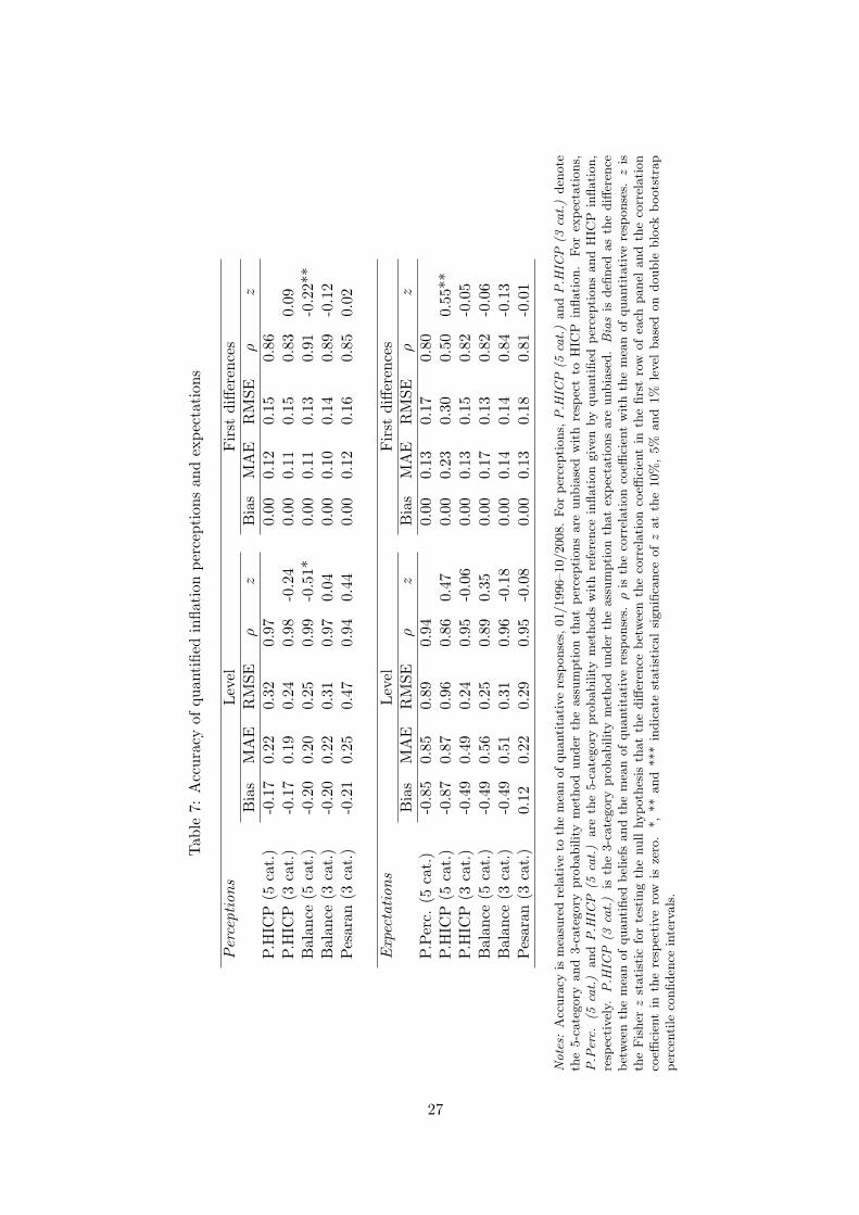
Table 7 summarizes the results. The underlying series are plotted in Figures A.4 and A.5

in the Appendix. All statistics are provided for levels and first differences. The last column

in each panel shows the Fisher z statistic for testing the null hypothesis that the difference

between the correlation coefficient in the first row of each panel (ρ1) and the correlation coeffi-

cient in the respective row (ρ2) is zero. Since the quantified series and the mean quantitative

beliefs are highly persistent, the discussion focuses on results for first differences.32 These

results are not subject to spurious regression problems as the first differences are stationary.

However, the results on the significance of correlation are mostly consistent for levels and first

differences.

Panel 1 of Table 7 indicates that in terms of correlation with the mean of quantitative

perceptions, all quantification methods perform well. The correlation in first differences is 0.86

for the series generated with the 5-category probability method. The 3-category probability

method generates virtually identical results. Interestingly, the 5-category and 3-category

balance statistics are more accurate, with correlation coefficients of 0.91 and 0.89, respectively.

The z-statistic indicates that the correlation coefficient for the 5-category balance statistic is

significantly higher than the correlation coefficient for the 5-category probability method.

Regarding expectations, panel 2 of Table 7 shows that the accuracy of the 5-category

probability method depends on the imposed reference inflation. Employing quantified per-

31Matlab codes are available from the author. The double moving block bootstrap of the percentile confidenceinterval is based on 1,000 first level replications and 2,500 second level replications and a block size of 5. SeeEfron and Tibshirani (1993) for a description of the method.

32Employing an Augmented Dickey-Fuller test the null hypothesis of a unit root cannot be rejected on the10% level for all actual and quantified mean series.

26

Tab

le7:

Accuracy

ofquan

tified

inflationperceptionsandexpectations

Perceptions

Level

First

differences

Bias

MAE

RMSE

ρz

Bias

MAE

RMSE

ρz

P.H

ICP

(5cat.)

-0.17

0.22

0.32

0.97

0.00

0.12

0.15

0.86

P.H

ICP

(3cat.)

-0.17

0.19

0.24

0.98

-0.24

0.00

0.11

0.15

0.83

0.09

Balan

ce(5

cat.)

-0.20

0.20

0.25

0.99

-0.51*

0.00

0.11

0.13

0.91

-0.22**

Balan

ce(3

cat.)

-0.20

0.22

0.31

0.97

0.04

0.00

0.10

0.14

0.89

-0.12

Pesaran

(3cat.)

-0.21

0.25

0.47

0.94

0.44

0.00

0.12

0.16

0.85

0.02

Expectations

Level

First

differences

Bias

MAE

RMSE

ρz

Bias

MAE

RMSE

ρz

P.Perc.

(5cat.)

-0.85

0.85

0.89

0.94

0.00

0.13

0.17

0.80

P.H

ICP

(5cat.)

-0.87

0.87

0.96

0.86

0.47

0.00

0.23

0.30

0.50

0.55**

P.H

ICP

(3cat.)

-0.49

0.49

0.24

0.95

-0.06

0.00

0.13

0.15

0.82

-0.05

Balan

ce(5

cat.)

-0.49

0.56

0.25

0.89

0.35

0.00

0.17

0.13

0.82

-0.06

Balan

ce(3

cat.)

-0.49

0.51

0.31

0.96

-0.18

0.00

0.14

0.14

0.84

-0.13

Pesaran

(3cat.)

0.12

0.22

0.29

0.95

-0.08

0.00

0.13

0.18

0.81

-0.01

Notes:

Accuracy

ismeasuredrelativeto

themeanofquantitativeresp

onses,

01/1996–10/2008.Forperceptions,

P.H

ICP

(5cat.)andP.H

ICP

(3cat.)den

ote

the5-category

and

3-category

probabilitymethod

under

theassumption

thatperceptionsare

unbiased

with

resp

ectto

HIC

Pinflation.

Forexpectations,

P.P

erc.

(5cat.)

andP.H

ICP

(5cat.)

are

the5-category

probabilitymethodswithreference

inflationgiven

byquantified

perceptionsandHIC

Pinflation,

resp

ectively.

P.H

ICP

(3cat.)

isthe3-category

probabilitymethodunder

theassumptionthatexpectationsare

unbiased.Biasis

defi

ned

asthedifferen

cebetweenthemeanofquantified

beliefs

andthemeanofquantitativeresp

onses.

ρis

thecorrelationcoeffi

cien

twiththemeanofquantitativeresp

onses.

zis

theFisher

zstatistic

fortestingthenullhypothesis

thatthedifferen

cebetweenthecorrelationco

efficien

tin

thefirstrow

ofeach

panel

andthecorrelation

coeffi

cien

tin

theresp

ectiverow

iszero.*,**and***indicate

statisticalsignificance

ofzatthe10%,5%

and1%

level

basedondouble

block

bootstrap

percentile

confiden

ceintervals.

27

ceptions generates significantly better results than employing actual HICP inflation, as the

z-statistic indicates. The correlation coefficients are 0.80 and 0.50, respectively. The most

accurate method for quantifying inflation expectations is again a balance statistic. Moreover,

the 3-category regression approach is slightly more accurate than the 5-category probability

method. These differences are not statistically significant, however. Results for the sample

01/2002–10/2008 in Table A.1 confirm these findings.

In sum, all quantification methods generate series that are highly correlated with the cross-

sectional mean of quantitative inflation perceptions. The 5-category balance statistic tracks

actual quantitative perceptions most accurately. For expectations, none of the alternative

methods performs significantly better than the 5-category probability method with reference

inflation given by quantified perceptions. The reasonable performance of the probability

method is in contrast to findings of Batchelor (1986) for the U.S.33 However, the 5-category

probability method may perform weakly to quantify expectations, depending on the chosen

reference inflation. Moreover, the similar accuracy of the 5-category probability method and

the 3-category methods signals that the 5-category probability method does not efficiently

use information from positive response categories.

4.2 Heterogeneity of Beliefs

The cross-sectional heterogeneity of beliefs is subject to increasing research in macroeco-

nomics. This section investigates how to best infer cross-sectional heterogeneity from qual-

itative survey data. Cross-sectional heterogeneity is measured by the standard deviation of

quantitative beliefs.

The 5-category probability method not only allows to identify the mean but also the

standard deviation of the fitted normal distribution given by Equation (A.4). In addition, I

consider four alternative measures of heterogeneity. The first alternative is implied standard

deviation from the 3-category probability method, given by Equation (A.9). The second

33Batchelor (1986) documents that the quantified series do not predict the direction of change in mean quan-titative responses. In the present case, a comparison of signs confirms the high correlation in first differences.For inflation perceptions, the balance statistic and the probability method indicate the correct direction ofchange of the mean quantitative response in 131 and 129 out of 153 months, for expectations in 121 and 120months.

28

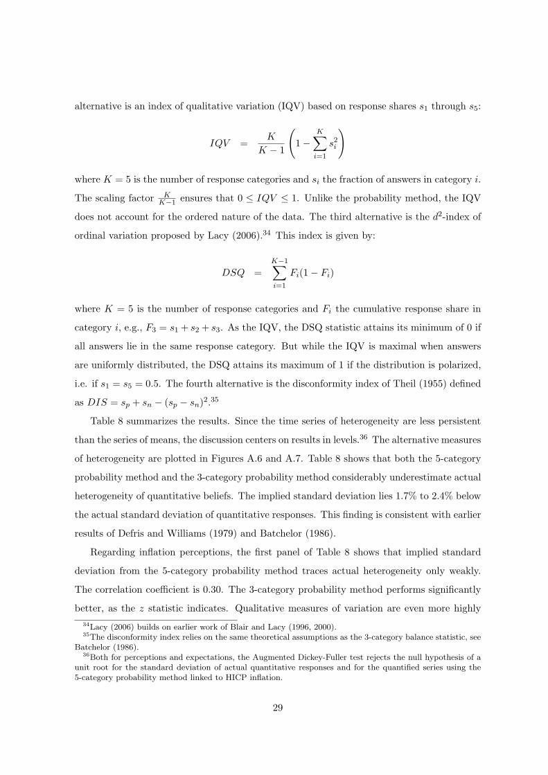
alternative is an index of qualitative variation (IQV) based on response shares s1 through s5:

IQV =K

K − 1

(1−

K∑i=1

s2i

)

where K = 5 is the number of response categories and si the fraction of answers in category i.

The scaling factor KK−1 ensures that 0 ≤ IQV ≤ 1. Unlike the probability method, the IQV

does not account for the ordered nature of the data. The third alternative is the d2-index of

ordinal variation proposed by Lacy (2006).34 This index is given by:

DSQ =

K−1∑i=1

Fi(1− Fi)

where K = 5 is the number of response categories and Fi the cumulative response share in

category i, e.g., F3 = s1 + s2 + s3. As the IQV, the DSQ statistic attains its minimum of 0 if

all answers lie in the same response category. But while the IQV is maximal when answers

are uniformly distributed, the DSQ attains its maximum of 1 if the distribution is polarized,

i.e. if s1 = s5 = 0.5. The fourth alternative is the disconformity index of Theil (1955) defined

as DIS = sp + sn − (sp − sn)2.35

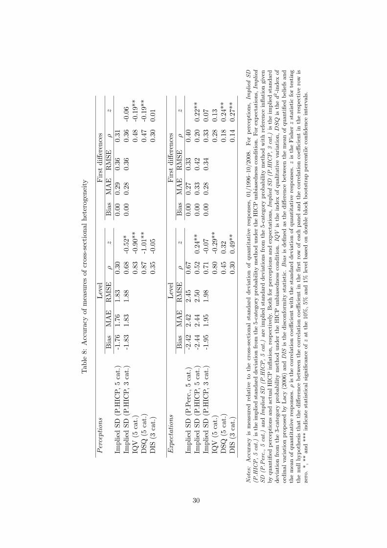
Table 8 summarizes the results. Since the time series of heterogeneity are less persistent

than the series of means, the discussion centers on results in levels.36 The alternative measures

of heterogeneity are plotted in Figures A.6 and A.7. Table 8 shows that both the 5-category

probability method and the 3-category probability method considerably underestimate actual

heterogeneity of quantitative beliefs. The implied standard deviation lies 1.7% to 2.4% below

the actual standard deviation of quantitative responses. This finding is consistent with earlier

results of Defris and Williams (1979) and Batchelor (1986).

Regarding inflation perceptions, the first panel of Table 8 shows that implied standard

deviation from the 5-category probability method traces actual heterogeneity only weakly.

The correlation coefficient is 0.30. The 3-category probability method performs significantly

better, as the z statistic indicates. Qualitative measures of variation are even more highly

34Lacy (2006) builds on earlier work of Blair and Lacy (1996, 2000).35The disconformity index relies on the same theoretical assumptions as the 3-category balance statistic, see

Batchelor (1986).36Both for perceptions and expectations, the Augmented Dickey-Fuller test rejects the null hypothesis of a

unit root for the standard deviation of actual quantitative responses and for the quantified series using the5-category probability method linked to HICP inflation.

29

Tab

le8:

Accuracy

ofmeasuresofcross-sectionalheterogeneity

Perceptions

Level

First

differences

Bias

MAE

RMSE

ρz

Bias

MAE

RMSE

ρz

Implied

SD

(P.H

ICP,5cat.)

-1.76

1.76

1.83

0.30

0.00

0.29

0.36

0.31

Implied

SD

(P.H

ICP,3cat.)

-1.83

1.83

1.88

0.68

-0.52*

0.00

0.28

0.36

0.36

-0.06

IQV

(5cat.)

0.83

-0.90**

0.48

-0.19**

DSQ

(5cat.)

0.87

-1.01**

0.47

-0.19**

DIS

(3cat.)

0.35

-0.05

0.30

0.01

Expectations

Level

First

differences

Bias

MAE

RMSE

ρz

Bias

MAE

RMSE

ρz

Implied

SD

(P.Perc.,5cat.)

-2.42

2.42

2.45

0.67

0.00

0.27

0.33

0.40

Implied

SD

(P.H

ICP,5cat.)

-2.44

2.44

2.50

0.52

0.24**

0.00

0.33

0.42

0.20

0.22**

Implied

SD

(P.H

ICP,3cat.)

-1.95

1.95

1.98

0.71

-0.07

0.00

0.28

0.34

0.33

0.07

IQV

(5cat.)

0.80

-0.29**

0.28

0.13

DSQ

(5cat.)

0.45

0.32

0.18

0.24**

DIS

(3cat.)

0.30

0.49**

0.14

0.27**

Notes:

Accuracy

ismeasured

relativeto

thecross-sectionalstandard

deviation

ofquantitativeresp

onses,

01/1996–10/2008.

Forperceptions,

Implied

SD

(P.H

ICP,5cat.)istheim

plied

standard

deviationfrom

the5-category

probabilitymethodunder

theHIC

Punbiasednesscondition.Forexpectations,

Implied

SD

(P.P

erc.,5cat.)andIm

plied

SD

(P.H

ICP,5cat.)are

implied

standard

deviationsfrom

the5-category

probabilitymethodwithreference

inflationgiven

byquantified

perceptionsandactualHIC

Pinflation,resp

ectively.

Both

forperceptionsandexpectations,

Implied

SD

(P.H

ICP,3cat.)istheim

plied

standard

deviationfrom

the3-category

probabilitymethodunder

theHIC

Punbiasednesscondition.IQ

Vis

theindex

ofqualitativeva

riation,DSQ

isthed2-index

of

ordinalvariationproposedbyLacy

(2006)andDIS

isthedisconform

itystatistic.Biasis

defi

ned

asthedifferen

cebetweenthemeanofquantified

beliefs

and

themeanofquantitativeresp

onses.

ρis

thecorrelationcoeffi

cien

twiththestandard

deviationofquantitativeresp

onses.

zis

theFisher

zstatistic

fortesting

thenullhypothesis

thatthedifferen

cebetweenthecorrelationco

efficien

tin

thefirstrow

ofeach

panel

andthecorrelationcoeffi

cien

tin

theresp

ectiverow

iszero.*,**and***indicate

statisticalsignificance

ofzatthe10%,5%

and1%

level

basedondouble

block

bootstrappercentile

confiden

ceintervals.

30

correlated with the standard deviation of quantitative perceptions. The correlation coefficients

of the IQV and the DSQ are 0.83 and 0.87, respectively. The performance of the 3-category

disconformity index is substantially lower, its correlation with actual standard deviation of

quantitative responses is similar to the 5-category probability method.

The implied standard deviation from the 5-category probability method performs better

for quantifying heterogeneity of inflation expectations, as the second panel of Table 8 indicates.

Again, the correlation depends on the choice of reference inflation. Employing actual HICP

inflation instead of quantified perceptions reduces the correlation coefficient significantly from

0.67 to 0.52. The implied standard deviation of the 3-category approach is about as accurate

as the 5-category probability method with reference inflation given by quantified perceptions.

The IQV most closely tracks actual heterogeneity of quantitative responses. Its correlation

with actual standard deviation is 0.80, which is significantly higher than the correlation of the

5-category probability method. Unlike for perceptions, the DSQ statistic is only moderately

correlated with actual heterogeneity. Even lower is the correlation for the disconformity

index, which is in line with earlier findings of Batchelor (1986). Results for first differences

are broadly consistent, with the exception that for quantifying expectations the IQV does

not outperform other methods anymore. Results for the shorter sample spanning 01/2002–

10/2008 in Table A.2 confirm the relatively high accuracy of the IQV compared to other

methods.37

In sum, these results suggest that while the probability method is relatively accurate in de-

scribing the central tendency, it is considerably less accurate in capturing cross-sectional het-

erogeneity. Moreover, the 3-category probability method performs better than the 5-category

method, which is consistent with findings of the previous section.38 The IQV generally domi-

nates the other methods in terms of correlation with the cross-sectional standard deviation of

quantitative beliefs. The DSQ is only accurate for quantifying the heterogeneity of inflation

perceptions. A possible interpretation of this result is that the IQV is less distorted by the

lack of order in qualitative inflation expectations than the DSQ index.

37Note that in this sample the probability method gains relative accuracy for quantifying inflation expecta-tions. I have also assessed accuracy of the square root of the index of qualitative variation, the square rootof the DSQ-statistic and the square root of the disconformity index. The correlations with actual standarddeviation of survey responses do not significantly change, both in their absolute level and relative ordering.

38The reasonable performance of the 3-category probability method also reinforces the results of Dasguptaand Lahiri (1993) who show that implied dispersion from the 3-category method is useful for predicting businesscycle turning points.

31

5 Which Quantification Method Should Be Used?

The assumptions of the 5-category probability method can be individually and jointly rejected.

Moreover, the estimated response schemes indicate that qualitative inflation expectations

are not strictly increasing in quantitative expectations since positive responses are given

relative to perceived inflation. Both for perceptions and expectations of inflation, however,

the response scheme estimates indicate that three separate positive categories S3, S4 and S5

contain additional information over just one positive category.

Despite the violation of theoretical assumptions, the accuracy of the 5-category probability

method for quantifying the cross-sectional mean of inflation perceptions is high. The relative

performance of the 3-category probability method indicates, however, that the 5-category

method does not efficiently use the additional information from three positive response cate-

gories. The most accurate method is the 5-category balance statistic.

For quantifying the cross-sectional mean of inflation expectations, the accuracy of the

5-category probability method largely depends on the chosen reference inflation πrt . Employ-

ing quantified inflation perceptions yields significantly more accurate results than employing

actual HICP inflation. At first sight this finding is inconsistent with the zero correlation of

quantified perceptions and reference inflation during the full sample as documented in Section

3.5. But as Figure 2 indicates, the relation between quantified perceptions and reference in-

flation becomes stronger towards the end of the sample period. The correlation coefficient of

reference inflation and quantified perceptions increases to 0.46 during 2002–2008. In particu-

lar, quantified perceptions surge in 2007 and 2008, while reference inflation increases to about

6%. This suggests that the 5-category probability method with quantified perceptions as

reference inflation will gain relative accuracy once inflation perceptions substantially diverge

from actual inflation.39

It remains the question why the simple balance statistic tends to trace mean beliefs even

more closely than the 5-category probability method. Table 9 provides a possible expla-

nation. The table shows the mean of quantitative responses conditional on the qualitative

response. Conditional means of actual quantitative responses are compared to the imposed

conditional means of the balance statistic and of the 5-category probability method. The

imposed conditional means are scaled to match the mean and variance of actual conditional

39This is the case, e.g., around the euro cash changeover in 2002 (ECB, 2005).

32

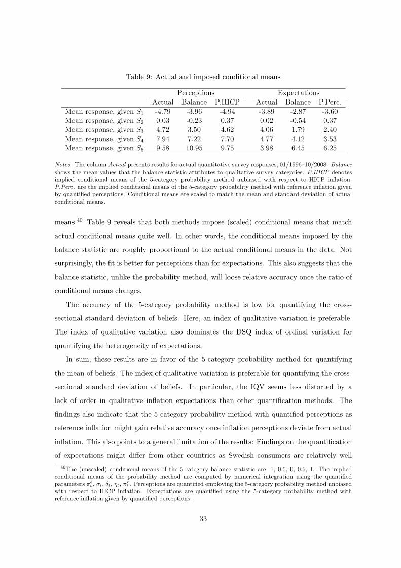
Table 9: Actual and imposed conditional means

Perceptions ExpectationsActual Balance P.HICP Actual Balance P.Perc.

Mean response, given S1 -4.79 -3.96 -4.94 -3.89 -2.87 -3.60Mean response, given S2 0.03 -0.23 0.37 0.02 -0.54 0.37Mean response, given S3 4.72 3.50 4.62 4.06 1.79 2.40Mean response, given S4 7.94 7.22 7.70 4.77 4.12 3.53Mean response, given S5 9.58 10.95 9.75 3.98 6.45 6.25

Notes: The column Actual presents results for actual quantitative survey responses, 01/1996–10/2008. Balanceshows the mean values that the balance statistic attributes to qualitative survey categories. P.HICP denotesimplied conditional means of the 5-category probability method unbiased with respect to HICP inflation.P.Perc. are the implied conditional means of the 5-category probability method with reference inflation givenby quantified perceptions. Conditional means are scaled to match the mean and standard deviation of actualconditional means.

means.40 Table 9 reveals that both methods impose (scaled) conditional means that match

actual conditional means quite well. In other words, the conditional means imposed by the

balance statistic are roughly proportional to the actual conditional means in the data. Not

surprisingly, the fit is better for perceptions than for expectations. This also suggests that the

balance statistic, unlike the probability method, will loose relative accuracy once the ratio of

conditional means changes.

The accuracy of the 5-category probability method is low for quantifying the cross-

sectional standard deviation of beliefs. Here, an index of qualitative variation is preferable.

The index of qualitative variation also dominates the DSQ index of ordinal variation for

quantifying the heterogeneity of expectations.

In sum, these results are in favor of the 5-category probability method for quantifying

the mean of beliefs. The index of qualitative variation is preferable for quantifying the cross-

sectional standard deviation of beliefs. In particular, the IQV seems less distorted by a

lack of order in qualitative inflation expectations than other quantification methods. The

findings also indicate that the 5-category probability method with quantified perceptions as

reference inflation might gain relative accuracy once inflation perceptions deviate from actual

inflation. This also points to a general limitation of the results: Findings on the quantification

of expectations might differ from other countries as Swedish consumers are relatively well

40The (unscaled) conditional means of the 5-category balance statistic are -1, 0.5, 0, 0.5, 1. The impliedconditional means of the probability method are computed by numerical integration using the quantifiedparameters πe

t , σt, δt, ηt, πrt . Perceptions are quantified employing the 5-category probability method unbiased

with respect to HICP inflation. Expectations are quantified using the 5-category probability method withreference inflation given by quantified perceptions.

33

informed about actual HICP inflation.

6 Conclusion

This paper assesses the validity and accuracy of the 5-category probability method for quantifying

household perceptions and expectations of inflation. The analysis capitalizes on jointly avail-

able qualitative and quantitative response data from the Swedish Consumer Tendency Sur-

vey. Relying on monthly household-level data covering 01/1996–10/2008, the theoretical

assumptions of the 5-category probability method are individually and jointly tested and re-

jected. Maximum likelihood estimations of unrestricted response schemes indicate that the

actual response scheme is neither symmetric nor homogeneous across individuals. Moreover,

it is found that qualitative inflation expectations are formed relative to inflation perceptions,

which is a direct result of survey design. An important consequence is that the conditional

mean of quantitative inflation expectations is not monotonously rising in qualitative response

categories. Furthermore, quantitative beliefs are not normally distributed and cannot be rec-

onciled with a noncentral t distribution either. The usual assumptions on the reference rate

of inflation (the “moderate” rate of inflation) are shown to be at odds with the data.

Nevertheless, the accuracy of the 5-category probability method in terms of correlation

with the mean of actual quantitative beliefs is high. For quantifying inflation expectations the

accuracy of the method strongly depends on the identifying restriction imposed by the choice

of reference inflation. Relying on double block bootstrap confidence intervals for Fisher’s z

statistic, it is shown that setting reference inflation equal to previously quantified inflation

perceptions yields significantly better results than setting reference inflation equal to actual

inflation. Nevertheless, the 5-category probability method is not more accurate than the

balance statistic and the 3-category probability method. This suggests that the 5-category

probability method does not efficiently use information from positive qualitative response

categories. In sum, the results are still in favor of the 5-category probability method. In

particular, the 5-category probability method with quantified perceptions as reference infla-

tion might gain relative accuracy once inflation perceptions substantially deviate from actual

inflation. The most accurate measure of the cross-sectional standard deviation of beliefs is

the index of qualitative variation.

The findings for Sweden suggest a number of avenues for further research. To exploit the

34

additional information from three positive response categories, research is needed on how to

identify the reference rate of inflation. Moreover, a non-parametric analysis should generate

further insights that will help to improve the imposed response scheme and distribution.

Looking ahead, implications for survey design should also be discussed in more depth. The

results for Sweden indicate that it is difficult to efficiently handle the relative nature of the

positive qualitative responses about inflation expectations. Obvious alternative survey designs

include to adopt the same response scheme for expectations as currently in use for perceptions

or to directly ask for quantitative responses in the first place.

35

References

Aalto-Setala, V. (2006): “Why Do Consumers Believe That the Euro Raised Prices?,”

International Journal of Consumer Studies, 30(2), 202–206.

Anderson, O. (1952): “The Business Test of the IFO-Institute for Economic Research

Munich, and Its Theoretical Model,” Revue de l’Institut International de Statistique, 20,

1–17.

Aucremanne, L., M. Collin, and T. Stragier (2007): “Assessing the Gap Between

Observed and Perceived Inflation in the Euro Area: Is the Credibility of the HICP at

Stake?,” National Bank of Belgium Working Paper 112.

Batchelor, R. A. (1982): “Aggregate Expectations Under the Stable Laws,” Journal of

Econometrics, 16(2), 199–210.

(1986): “Quantitative v. Qualitative Measures of Inflation Expectations,” Oxford

Bulletin of Economics and Statistics, 48(2), 99–120.

Batchelor, R. A., and P. Dua (1987): “The Accuracy and Rationality of UK Inflation

Expectations: Some Quantitative Evidence,” Applied Economics, 19(6), 819–828.

Batchelor, R. A., and A. B. Orr (1988): “Inflation Expectations Revisited,” Economica,

55(219), 317–331.

Berk, J. M. (1999): “Measuring Inflation Expectations: A Survey Data Approach,” Applied

Economics, 31(11), 1467–1480.

Blair, J., and M. G. Lacy (1996): “Measures of Variation for Ordinal Data as Functions

of the Cumulative Distribution,” Perceptual and Motor Skills, 82(2), 411–418.

(2000): “Statistics of Ordinal Variation,” Sociological Methods & Research, 28(3),

251–280.

Bryan, M. F., and S. Palmqvist (2006): “Testing Near-Rationality Using Detailed Survey

Data,” Sveriges Riksbank Research Paper Series.

Bryan, M. F., and G. Venkatu (2001a): “The Curiously Different Inflation Perspectives

of Men and Women,” Federal Reserve Bank of Cleveland Economic Commentary Series.

36

(2001b): “The Demographics of Inflation Opinion Surveys,” Federal Reserve Bank

of Cleveland Economic Commentary Series.

Carlson, J. A. (1975): “Are Price Expectations Normally Distributed?,” Journal of the

American Statistical Association, 352, 749–754.

Carlson, J. A., and M. Parkin (1975): “Inflation Expectations,” Economica, 42(166),

123–138.

Dasgupta, S., and K. Lahiri (1992): “A Comparative Study of Alternative Methods of

Quantifying Qualitative Survey Responses Using NAPM Data,” Journal of Business &

Economic Statistics, 10(4), 391–400.

(1993): “On the Use of Dispersion Measures From NAPM Surveys in Business Cycle

Forecasting,” Journal of Forecasting, 12(3-4), 239–253.

Defris, L. V., and R. A. Williams (1979): “Quantitative Versus Qualitative Measures

of Price Expectations: The Evidence From Australian Consumer Surveys,” Economics

Letters, 2(2), 169–173.

Doehring, B., and A. Mordonu (2007): “What Drives Inflation Perceptions? A Dynamic

Panel Data Analysis,” European Commission Economic Papers 284.

Dopke, J., J. Dovern, U. Fritsche, and J. Slacalek (2008): “The Dynamics of Euro-

pean Inflation Expectations,” B.E. Journal of Macroeconomics, 8(1).

Driver, R., and R. Windram (2007): “Public Attitudes to Inflation and Interest Rates,”

Bank of England Quarterly Bulletin, 47(2), 208–223.

Dziuda, W., and G. Mastrobuoni (2006): “The Euro Changeover and Its Effects on Price

Transparency and Inflation,” Working Paper 26, Collegio Carlo Alberto.

ECB (2005): “Consumers’ Inflation Perceptions: Still At Odds With Official Statistics?,”

ECB Monthly Bulletin, (4), 30–32.

Efron, B., and R. J. Tibshirani (1993): An Introduction to the Bootstrap. Chapman &

Hall.

37

Ehrmann, M. (2006): “Rational Inattention, Inflation Developments and Perceptions After

the Euro Cash Changeover,” ECB Working Paper 588, European Central Bank.

European Commission (2007): The Joint Harmonised EU Programme of Business and

Consumer Surveys: User Guide, European Commission, Directorate-General for Economic

and Financial Affairs.

Fluch, M., and H. Stix (2007): “The Development of Euro Prices - Subjective Perception

and Empirical Facts,” Monetary Policy and the Economy (OeNB), 07(1), 55–84.

Forsells, M., and G. Kenny (2004): “Survey Expectations, Rationality and the Dynamics

of Euro Area Inflation,” Journal of Business Cycle Measurement and Analysis, 1(1), 13–41.

GfK (2002): Consumer Tendency Survey, GfK Sweden, Stockholm, Sweden.

Henzel, S., and T. Wollmershauser (2005): “Quantifying Inflation Expectations With

the Carlson-Parkin Method: A Survey-based Determination of the Just Noticeable Differ-

ence,” Journal of Business Cycle Measurement and Analysis, 2(3).

Jonung, L., and D. Laidler (1988): “Are Perceptions of Inflation Rational? Some Evi-

dence for Sweden,” American Economic Review, 78(5), 1080–1087.

Lacy, M. G. (2006): “An Explained Variation Measure for Ordinal Response Models With

Comparisons to Other Ordinal R2 Measures,” Sociological Methods & Research, 34(4), 469–

520.

Lahiri, K., and C. Teigland (1987): “On the Normality of Probability Distributions of

Inflation and GNP Forecasts,” International Journal of Forecasting, 3(2), 269–279.

Lamla, M. J., and S. M. Lein (2008): “The Role of Media for Consumers’ Inflation

Expectation Formation,” KOF Working Papers 201, ETH Zurich.

Lein, S. M., and T. Maag (2008): “The Formation of Inflation Perceptions — Some

Empirical Facts for European Countries,” KOF Working Papers 204, ETH Zurich.

Mudholkar, G. S. (2006): “Fisher’s z-Transformation,” in Encyclopedia of Statistical Sci-

ences, ed. by S. Kotz, C. B. Read, N. Balakrishnan, and B. Vidakovic. Wiley.

38

Nardo, M. (2003): “The Quantification of Qualitative Survey Data: A Critical Assessment,”

Journal of Economic Surveys, 17, 645–668.

Palmqvist, S., and L. Stromberg (2004): “Households’ Inflation Opinions - A Tale of

Two Surveys,” Sveriges Riksbank Economic Review, 4, 23–42.

Pesaran, M. H. (1987): The Limits to Rational Expectations. Blackwell.

Smith, J., and M. McAleer (1995): “Alternative Procedures for Converting Qualitative

Response Data to Quantitative Expectations: An Application to Australian Manufactur-

ing,” Journal of Applied Econometrics, 10(2), 165–185.

Theil, H. (1952): “On the Shape of Microvariables and the Munich Business Test,” Revue

de l’Institut International de Statistique, 20, 105–120.

(1955): “Recent Experiences With the Munich Business Test: An Expository Arti-

cle,” Econometrica, 23(2), 184–192.

Zavoina, W., and R. D. McKelvey (1975): “A Statistical Model for the Analysis of

Ordinal Level Dependent Variables,” Journal of Mathematical Sociology, 4, 103–120.

39

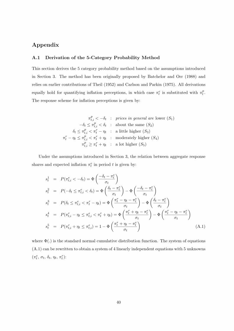
Appendix

A.1 Derivation of the 5-Category Probability Method

This section derives the 5 category probability method based on the assumptions introduced

in Section 3. The method has been originally proposed by Batchelor and Orr (1988) and

relies on earlier contributions of Theil (1952) and Carlson and Parkin (1975). All derivations

equally hold for quantifying inflation perceptions, in which case πet is substituted with πp

t .

The response scheme for inflation perceptions is given by:

πpt,i < −δt : prices in general are lower (S1)

−δt ≤ πpt,i < δt : about the same (S2)

δt ≤ πpt,i < πr

t − ηt : a little higher (S3)

πrt − ηt ≤ πp

t,i < πrt + ηt : moderately higher (S4)

πpt,i ≥ πr

t + ηt : a lot higher (S5)

Under the assumptions introduced in Section 3, the relation between aggregate response

shares and expected inflation πet in period t is given by:

s1t = P (πet,i < −δt) = Φ

(−δt − πe

t

σt

)s2t = P (−δt ≤ πe

t,i < δt) = Φ

(δt − πe

t

σt

)− Φ

(−δt − πe

t

σt

)s3t = P (δt ≤ πe

t,i < πrt − ηt) = Φ

(πrt − ηt − πe

t

σt

)− Φ

(δt − πe

t

σt

)s4t = P (πr

t,i − ηt ≤ πet,i < πr

t + ηt) = Φ

(πrt + ηt − πe

t

σt

)− Φ

(πrt − ηt − πe

t

σt

)s5t = P (πr

t,i + ηt ≤ πet,i) = 1− Φ

(πrt + ηt − πe

t

σt

)(A.1)

where Φ(.) is the standard normal cumulative distribution function. The system of equations

(A.1) can be rewritten to obtain a system of 4 linearly independent equations with 5 unknowns

(πet , σt, δt, ηt, π

rt ):

40

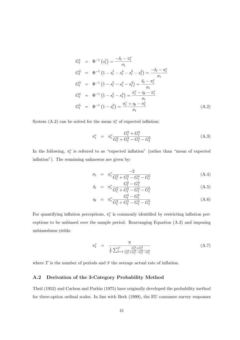
G1t = Φ−1

(s1t)=

−δt − πet

σt

G2t = Φ−1

(1− s5t − s4t − s3t − s2t

)=

−δt − πet

σt

G3t = Φ−1

(1− s5t − s4t − s3t

)=

δt − πet

σt

G4t = Φ−1

(1− s5t − s4t

)=

πrt − ηt − πe

t

σt

G5t = Φ−1

(1− s5t

)=

πrt + ηt − πe

t

σt(A.2)

System (A.2) can be solved for the mean πet of expected inflation:

πet = πr

t

G2t +G3

t

G2t +G3

t −G4t −G5

t

(A.3)

In the following, πet is referred to as “expected inflation” (rather than “mean of expected

inflation”). The remaining unknowns are given by:

σt = πrt

−2

G2t +G3

t −G4t −G5

t

(A.4)

δt = πrt

G2t −G3

t

G2t +G3

t −G4t −G5

t

(A.5)

ηt = πrt

G4t −G5

t

G2t +G3

t −G4t −G5

t

(A.6)

For quantifying inflation perceptions, πrt is commonly identified by restricting inflation per-

ceptions to be unbiased over the sample period. Rearranging Equation (A.3) and imposing

unbiasedness yields:

πrt =

π

1T

∑Tt=1

G2t+G3

t

G2t+G3

t−G4t−G5

t

(A.7)

where T is the number of periods and π the average actual rate of inflation.

A.2 Derivation of the 3-Category Probability Method

Theil (1952) and Carlson and Parkin (1975) have originally developed the probability method

for three-option ordinal scales. In line with Berk (1999), the EU consumer survey responses

41

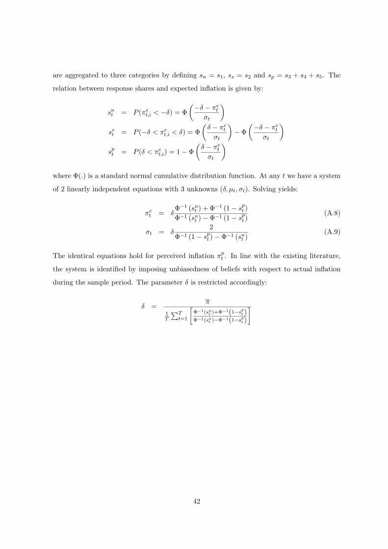
are aggregated to three categories by defining sn = s1, ss = s2 and sp = s3 + s4 + s5. The

relation between response shares and expected inflation is given by:

snt = P (πet,i < −δ) = Φ

(−δ − πe

t

σt

)sst = P (−δ < πe

t,i < δ) = Φ

(δ − πe

t

σt

)− Φ

(−δ − πe

t

σt

)spt = P (δ < πe

t,i) = 1− Φ

(δ − πe

t

σt

)

where Φ(.) is a standard normal cumulative distribution function. At any t we have a system

of 2 linearly independent equations with 3 unknowns (δ, µt, σt). Solving yields:

πet = δ

Φ−1 (snt ) + Φ−1 (1− spt )

Φ−1 (snt )− Φ−1 (1− spt )(A.8)

σt = δ2

Φ−1 (1− spt )− Φ−1 (snt )(A.9)

The identical equations hold for perceived inflation πpt . In line with the existing literature,

the system is identified by imposing unbiasedness of beliefs with respect to actual inflation

during the sample period. The parameter δ is restricted accordingly:

δ =π

1T

∑Tt=1

[Φ−1(snt )+Φ−1(1−spt )Φ−1(snt )−Φ−1(1−spt )

]

42

A.3 Further Results

43

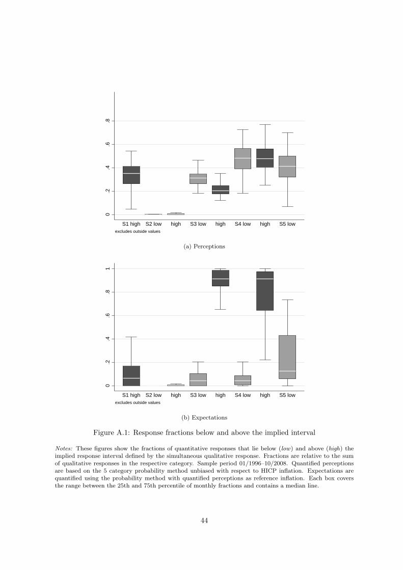
0.2

.4.6

.8

S1 high S2 low high S3 low high S4 low high S5 lowexcludes outside values

(a) Perceptions

0.2

.4.6

.81

S1 high S2 low high S3 low high S4 low high S5 lowexcludes outside values

(b) Expectations

Figure A.1: Response fractions below and above the implied interval

Notes: These figures show the fractions of quantitative responses that lie below (low) and above (high) theimplied response interval defined by the simultaneous qualitative response. Fractions are relative to the sumof qualitative responses in the respective category. Sample period 01/1996–10/2008. Quantified perceptionsare based on the 5 category probability method unbiased with respect to HICP inflation. Expectations arequantified using the probability method with quantified perceptions as reference inflation. Each box coversthe range between the 25th and 75th percentile of monthly fractions and contains a median line.

44

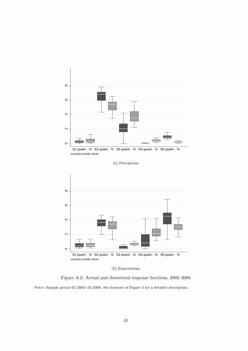
0.2

.4.6

.8

S1 quant. N S2 quant. N S3 quant. N S4 quant. N S5 quant. Nexcludes outside values

(a) Perceptions

0.2

.4.6

.8

S1 quant. N S2 quant. N S3 quant. N S4 quant. N S5 quant. Nexcludes outside values

(b) Expectations

Figure A.2: Actual and theoretical response fractions, 2002–2008

Notes: Sample period 01/2002–10/2008. See footnote of Figure 3 for a detailed description.

45

0.2

.4.6

.8

S1 high S2 low high S3 low high S4 low high S5 lowexcludes outside values

(a) Perceptions

0.2

.4.6

.81

S1 high S2 low high S3 low high S4 low high S5 lowexcludes outside values

(b) Expectations

Figure A.3: Response fractions below and above the implied interval, 2002–2008

Notes: Sample period 01/2002–10/2008. See footnote of Figure A.1 for a detailed description.

46

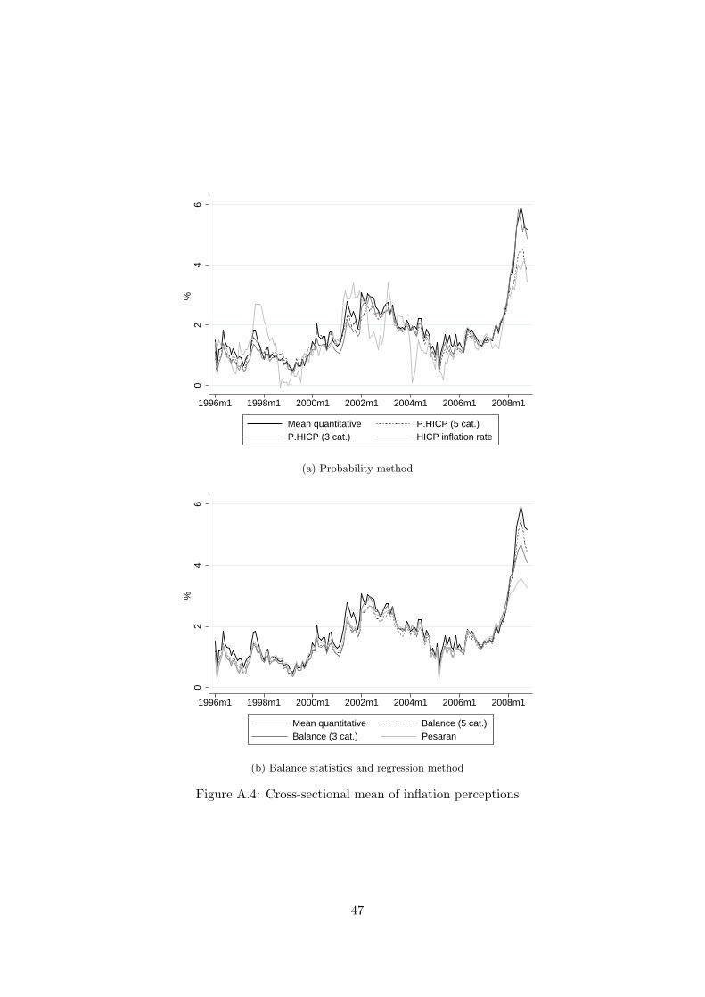
02

46

%

1996m1 1998m1 2000m1 2002m1 2004m1 2006m1 2008m1

Mean quantitative P.HICP (5 cat.)P.HICP (3 cat.) HICP inflation rate

(a) Probability method

02

46

%

1996m1 1998m1 2000m1 2002m1 2004m1 2006m1 2008m1

Mean quantitative Balance (5 cat.)Balance (3 cat.) Pesaran

(b) Balance statistics and regression method

Figure A.4: Cross-sectional mean of inflation perceptions

47

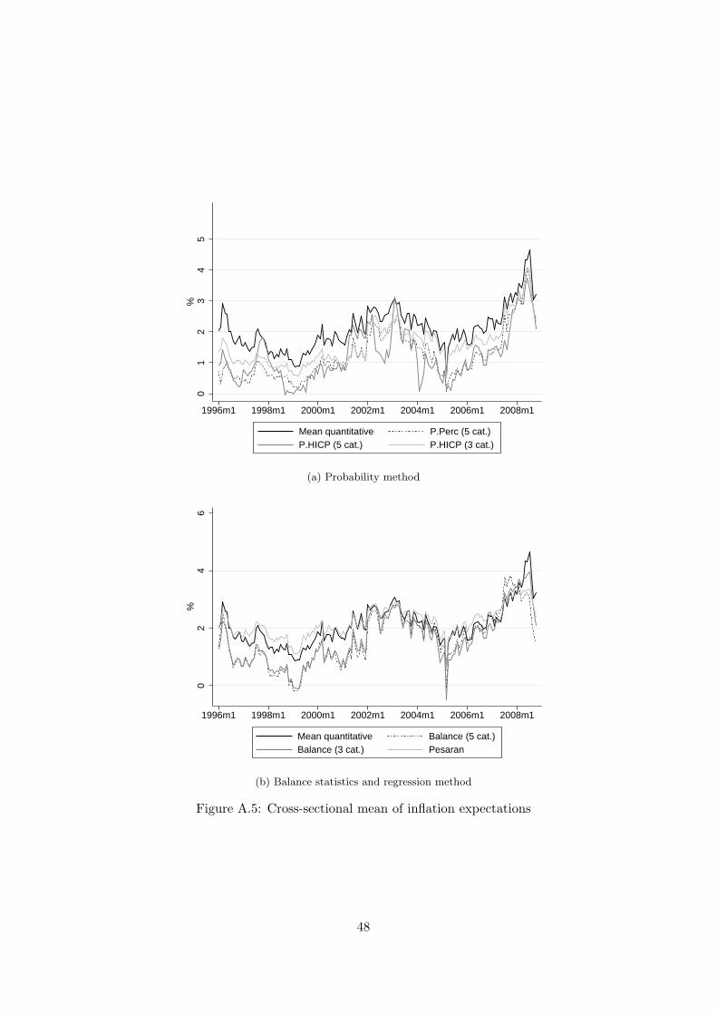
01

23

45

%

1996m1 1998m1 2000m1 2002m1 2004m1 2006m1 2008m1

Mean quantitative P.Perc (5 cat.)P.HICP (5 cat.) P.HICP (3 cat.)

(a) Probability method

02

46

%

1996m1 1998m1 2000m1 2002m1 2004m1 2006m1 2008m1

Mean quantitative Balance (5 cat.)Balance (3 cat.) Pesaran

(b) Balance statistics and regression method

Figure A.5: Cross-sectional mean of inflation expectations

48

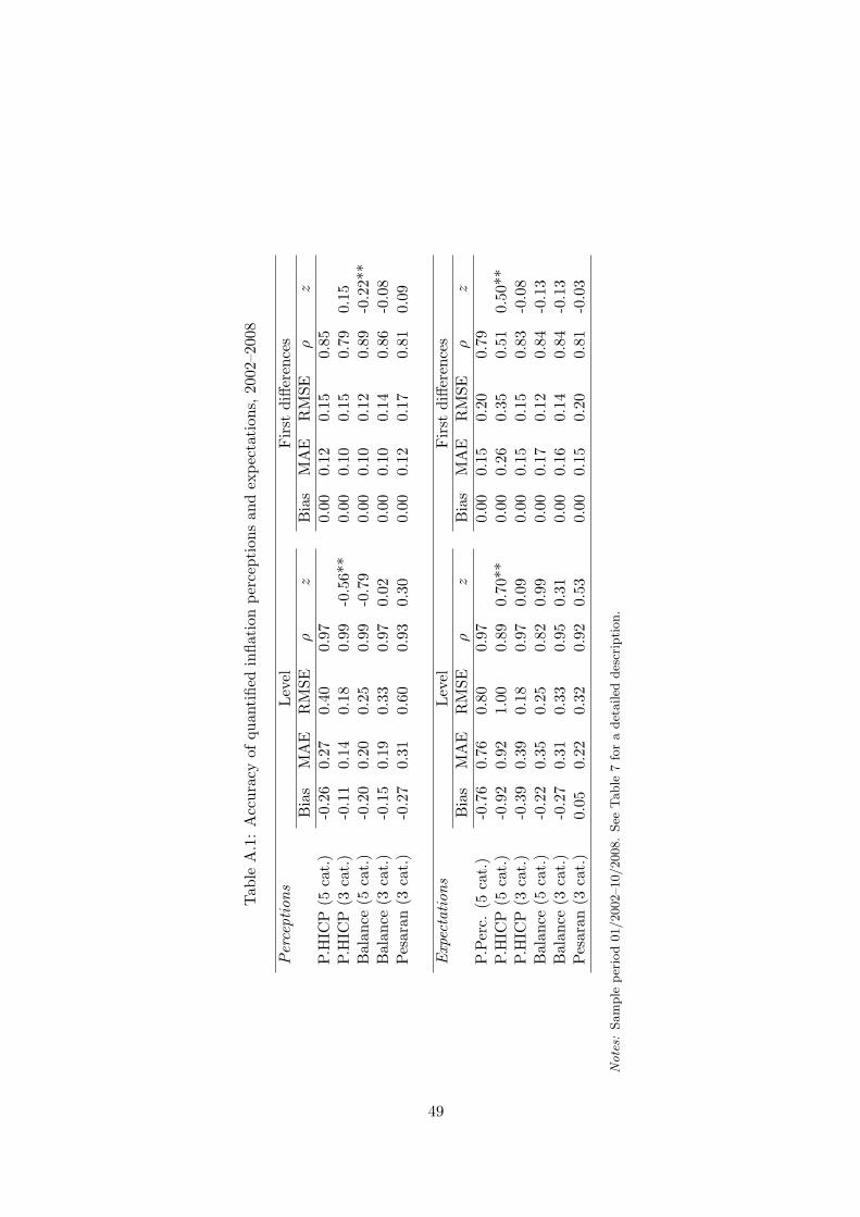
Tab

leA.1:Accuracy

ofquan

tified

inflationperceptionsandexpectations,

2002–2008

Perceptions

Level

First

differences

Bias

MAE

RMSE

ρz

Bias

MAE

RMSE

ρz

P.H

ICP

(5cat.)

-0.26

0.27

0.40

0.97

0.00

0.12

0.15

0.85

P.H

ICP

(3cat.)

-0.11

0.14

0.18

0.99

-0.56**

0.00

0.10

0.15

0.79

0.15

Balan

ce(5

cat.)

-0.20

0.20

0.25

0.99

-0.79

0.00

0.10

0.12

0.89

-0.22**

Balan

ce(3

cat.)

-0.15

0.19

0.33

0.97

0.02

0.00

0.10

0.14

0.86

-0.08

Pesaran

(3cat.)

-0.27

0.31

0.60

0.93

0.30

0.00

0.12

0.17

0.81

0.09

Expectations

Level

First

differences

Bias

MAE

RMSE

ρz

Bias

MAE

RMSE

ρz

P.Perc.

(5cat.)

-0.76

0.76

0.80

0.97

0.00

0.15

0.20

0.79

P.H

ICP

(5cat.)

-0.92

0.92

1.00

0.89

0.70**

0.00

0.26

0.35

0.51

0.50**

P.H

ICP

(3cat.)

-0.39

0.39

0.18

0.97

0.09

0.00

0.15

0.15

0.83

-0.08

Balan

ce(5

cat.)

-0.22

0.35

0.25

0.82

0.99

0.00

0.17

0.12

0.84

-0.13

Balan

ce(3

cat.)

-0.27

0.31

0.33

0.95

0.31

0.00

0.16

0.14

0.84

-0.13

Pesaran

(3cat.)

0.05

0.22

0.32

0.92

0.53

0.00

0.15

0.20

0.81

-0.03

Notes:

Sample

period01/2002–10/2008.See

Table

7foradetailed

description.

49

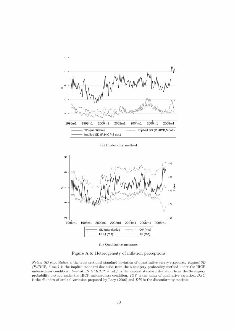
23

45

6%

1996m1 1998m1 2000m1 2002m1 2004m1 2006m1 2008m1

SD quantitative Implied SD (P.HICP,5 cat.)Implied SD (P.HICP,3 cat.)

(a) Probability method

0.2

.4.6

.8In

dex

23

45

6%

1996m1 1998m1 2000m1 2002m1 2004m1 2006m1 2008m1

SD quantitative IQV (rhs)DSQ (rhs) DC (rhs)

(b) Qualitative measures

Figure A.6: Heterogeneity of inflation perceptions

Notes: SD quantitative is the cross-sectional standard deviation of quantitative survey responses. Implied SD(P.HICP, 5 cat.) is the implied standard deviation from the 5-category probability method under the HICPunbiasedness condition. Implied SD (P.HICP, 3 cat.) is the implied standard deviation from the 3-categoryprobability method under the HICP unbiasedness condition. IQV is the index of qualitative variation, DSQis the d2-index of ordinal variation proposed by Lacy (2006) and DIS is the disconformity statistic.

50

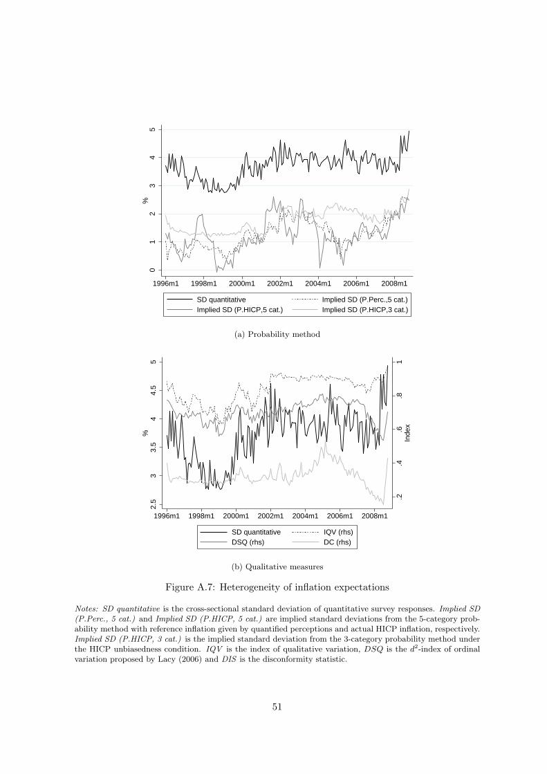
01

23

45

%

1996m1 1998m1 2000m1 2002m1 2004m1 2006m1 2008m1

SD quantitative Implied SD (P.Perc.,5 cat.)Implied SD (P.HICP,5 cat.) Implied SD (P.HICP,3 cat.)

(a) Probability method

.2.4

.6.8

1In

dex

2.5

33.

54

4.5

5%

1996m1 1998m1 2000m1 2002m1 2004m1 2006m1 2008m1

SD quantitative IQV (rhs)DSQ (rhs) DC (rhs)

(b) Qualitative measures

Figure A.7: Heterogeneity of inflation expectations

Notes: SD quantitative is the cross-sectional standard deviation of quantitative survey responses. Implied SD(P.Perc., 5 cat.) and Implied SD (P.HICP, 5 cat.) are implied standard deviations from the 5-category prob-ability method with reference inflation given by quantified perceptions and actual HICP inflation, respectively.Implied SD (P.HICP, 3 cat.) is the implied standard deviation from the 3-category probability method underthe HICP unbiasedness condition. IQV is the index of qualitative variation, DSQ is the d2-index of ordinalvariation proposed by Lacy (2006) and DIS is the disconformity statistic.

51

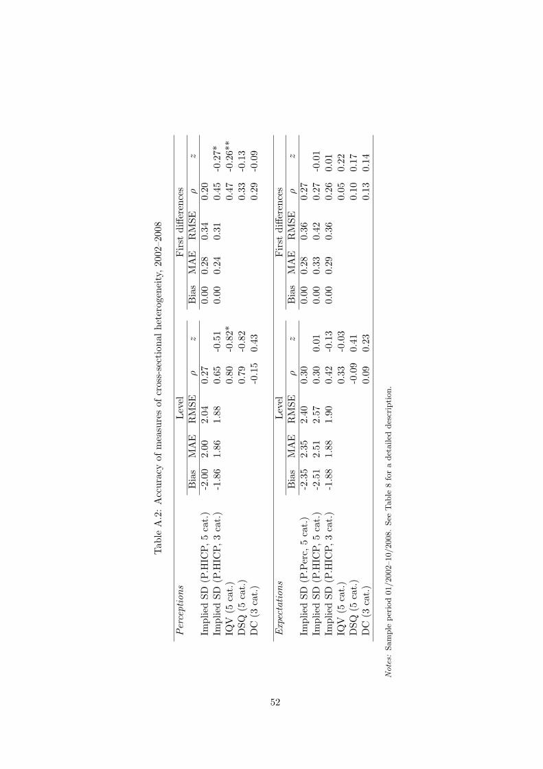
Tab

leA.2:Accuracy

ofmeasuresofcross-sectionalheterogeneity,2002–2008

Perceptions

Level

First

differences

Bias

MAE

RMSE

ρz

Bias

MAE

RMSE

ρz

Implied

SD

(P.H

ICP,5cat.)

-2.00

2.00

2.04

0.27

0.00

0.28

0.34

0.20

Implied

SD

(P.H

ICP,3cat.)

-1.86

1.86

1.88

0.65

-0.51

0.00

0.24

0.31

0.45

-0.27*

IQV

(5cat.)

0.80

-0.82*

0.47

-0.26**

DSQ

(5cat.)

0.79

-0.82

0.33

-0.13

DC

(3cat.)

-0.15

0.43

0.29

-0.09

Expectations

Level

First

differences

Bias

MAE

RMSE

ρz

Bias

MAE

RMSE

ρz

Implied

SD

(P.Perc,

5cat.)

-2.35

2.35

2.40

0.30

0.00

0.28

0.36

0.27

Implied

SD

(P.H

ICP,5cat.)

-2.51

2.51

2.57

0.30

0.01

0.00

0.33

0.42

0.27

-0.01

Implied

SD

(P.H

ICP,3cat.)

-1.88

1.88

1.90

0.42

-0.13

0.00

0.29

0.36

0.26

0.01

IQV

(5cat.)

0.33

-0.03

0.05

0.22

DSQ

(5cat.)

-0.09

0.41

0.10

0.17

DC

(3cat.)

0.09

0.23

0.13

0.14

Notes:

Sample

period01/2002–10/2008.See

Table

8foradetailed

description.

52