Nature of Overstabilities in Dilute Plasmas

KITP Lunch Talk, Apr 21, 2011

Tamara Bogdanović University of Maryland

Special thanks to KITP!

and collaborators Chris Reynolds and Steven Balbus

• ICM plasma is dilute and weakly magnetized-- charged particles are nearly freely streaming along the lines of magnetic field.

• Anisotropic conduction alters classic condition for convection.

• What are the implications for the ICM?

(Balbus 00)

Role of thermal conduction in dilute plasmas

arX

iv:a

stro

-ph/0

612195v1 7 D

ec 2

006

Draft version February 5, 2008Preprint typeset using LATEX style emulateapj v. 10/09/06

SATURATION OF THE MAGNETOTHERMAL INSTABILITY IN THREE DIMENSIONS

Ian J. Parrish and James M. Stone1

Department of Astrophysical Sciences, Princeton University, Princeton, NJ 08544Draft version February 5, 2008

ABSTRACT

In dilute astrophysical plasmas, thermal conduction is primarily along magnetic field lines, andtherefore highly anisotropic. As a result, the usual convective stability criterion is modified from acondition on entropy to a condition on temperature. For small magnetic fields or small wavenumbers,instability occurs in any atmosphere where the temperature and pressure gradients point in the samedirection. We refer to the resulting convective instability as the magnetothermal instability (MTI).We present fully three-dimensional simulations of the MTI and show that saturation results in anatmosphere with di!erent vertical structure, dependent upon the boundary conditions. When thetemperature at the boundary of the unstable layer is allowed to vary, the temperature gradient relaxesuntil the unstable region is almost isothermal. When the temperature at the boundary of the unstableregion is fixed, the magnetic field is reoriented to an almost vertical geometry as a result of buoyantmotions. This case exhibits more vigorous turbulence. In both cases the resulting saturated heat fluxis almost one-half of the value expected if the conduction were purely isotropic, !Q ! !"T/L, where! is the thermal conductivity, "T is the fixed temperature drop across the simulation domain, and Lis the temperature gradient scale length. The action of the MTI results in dynamical processes thatlead to significant transport perpendicular to the initial direction of the magnetic field. The resultingmagnetoconvection in both cases amplifies the magnetic field until it is almost in equipartition withsustained subsonic turbulence. These results are relevant to understanding measurements of thetemperature profiles of the intracluster medium of clusters of galaxies as well as the structure ofradiatively ine#cient accretion flows.Subject headings: accretion, accretion disks — convection — instabilities — MHD — galaxies: clusters

— stars: neutron

1. INTRODUCTION

In many astrophysical plasmas the collision frequencyis much smaller than the Larmor frequency, so that par-ticles spiral around the magnetic field lines for very longdistances between collisions. As a result, transport ofheat and momentum by thermal conduction and viscos-ity is highly anisotropic with respect to the magneticfield orientation. In a dilute magnetized plasma, elec-tron thermal conductivity parallel to the magnetic fieldis many orders of magnitude larger than both the per-pendicular electron conductivity and either componentof the ion conductivity provided " " #ee # $e, where#ee is the electron collision frequency, $e is the electrongyrofrequency, and " is the frequency of a physical pro-cess of interest. In this regime the plasma is decribedby the equations of magnetohydrodynamics (MHD) withthe addition of Braginskii anisotropic transport terms(Braginskii 1965). A Braginskii description is valid fordescribing processes where the mean free path is a sub-stantial fraction of the size of the system, but does notpermit an analysis of processes that occur on lengthscalesshorter than the mean free path, e.g. Landau damping.

These properties can have profound e!ects on theresulting plasma dynamics. A striking example isthe magnetothermal instability (MTI) (Balbus 2000;Parrish & Stone 2005). The magnetothermal instabil-ity occurs as a result of heat flow parallel to the mag-netic field in a statified atmosphere. The criterion

1 Program in Applied and Computational Mathematics, Prince-ton University, Princeton, NJ, 08544

for convective stability is modified from the well-knownSchwarzschild criterion ($S/$z > 0), where the entropy,S = p%!! , to the Balbus criterion ($ lnT/$z > 0), wherep and T are the pressure and temperature respectively.Atmospheres that have temperature (as opposed to en-tropy) profiles decreasing upwards are unstable to theMTI. In this situation the MTI is able to use the tem-perature gradient as a source of free energy for the insta-bility. The growth rate and saturation of this instabilityin two dimensions has been explored in Parrish & Stone(2005), hereafter PS. In PS we demonstrated that com-putationally measured growth rates match theoreticalestimates from a WKB theory for a variety of bound-ary and initial conditions. In addition, we showed thatMTI-unstable plasmas can produce vigorous convectivemotions and a significant advective heat flux. The satu-rated state for an adiabatic atmosphere in 2D was shownto result in an isothermal atmosphere.

We are motivated to study the nonlinear regime of themagnetothermal instability in three dimensions for sev-eral reasons. First, the saturation mechanism in threedimensions may be di!erent from two dimensions. Sec-ond, there is a potential for a magnetic dynamo in threedimensions. Finally, the nature of convection is knownto be intrinsically di!erent in three dimensions.

In this paper we present the saturation and heat trans-port properties of the MTI in three dimensions. Wefind the instability is capable of generating a magneticdynamo that greatly amplifies the initial field until itis roughly in equipartition with the fluid turbulent ki-netic energy. To estimate the e#ciency of heat trans-

RDCS 1259.9-2927

(Credit: NASA/CXC/SAO)

MHD instabilities and overstabilitiesL100 BALBUS & REYNOLDS Vol. 720

which bears direct comparison with Equation (26). Here, ther-mal conduction once again stabilizes radiative losses, but theHBI terms, when they are in a stable configuration relative tothe convective processes discussed by Q08, actively destabilizewave-like modes by reducing the suppression of thermal con-duction. In regions of sharp temperature gradients, the effectivereduction factor for conductive stabilization can be large. In-deed, in the chosen limit bz ! 1, we have R " O(bz). Note thatwavenumbers with vanishing k · b are unaffected by conductionand have an effective reduction factor of zero. In our example,these are horizontal fluid displacements along the magnetic fieldlines.

2.3.4. Destabilization of Wave Modes by a Negative Thermal Gradient

Next consider the case bz = 1, which would be HBI unstablein the case of an increasing outward temperature profile. But letus now assume that the temperature decreases outward. Thisconfiguration is HBI stable. With bz = 1, if we restrictedourselves only to the first two stability criteria, we wouldconclude that this configuration is also MTI stable. In fact,if the third stability criterion is imposed, this configuration issubject to an interesting and powerful overstability, driven byanisotropic thermal conduction, as we now show.

With bz = 1, we have K = #k2$ and our third criterion

inequality (30) becomes

! # 1!

T !T |P N2 + C!

N2 + gd ln T

dz

"> 0. (36)

Once again, the thermal conduction is affected by a “reductionfactor,” though here the reduction factor R% actively destabilizesrather than merely suppresses dissipative destabilization. Theabove inequality may be written as

T !T |P + "(k · b)2R% > 0, (37)

where

R% = 1 ##! # 1

!

d ln P

d ln T# 1

$#1

. (38)

The term inside the square brackets must always be positiveif N2 > 0, but if

1 <! # 1

!

d ln P

d ln T< 2, (39)

then R% < 0 and buoyant modes are overstable, even if there isno radiative loss term.

2.3.5. Summary

The MTI and HBI are evanescent instabilities present in diluteplasmas when anisotropic heat flux is included in the physics.The MTI is present when the thermal gradient decreases outwardand the field lines are insulating in the equilibrium configuration.When the field lines open, the MTI is stabilized. The HBI ispresent when the thermal gradient increases outward and thefield lines are open so that a heat flux is present in the equilibriumconfiguration. The action of the HBI is to close the field lines,which stabilizes the system.

We have found that the stable “end states” of these instabilitiesare subject to further overstabilities. In the case of the HBI,which is relevant for the cooling flow cores, a thermally unstableradiative loss function and closed field lines together manifest

dTdz

bz

Figure 1. Schematic map of the instabilities and overstabilities discussed in thiswork.

as over stable buoyant oscillations. In the case of the MTI, asufficiently steep (but classically convectively stable) outwardlydecreasing thermal gradient produces overstable buoyant waveswhen the magnetic field lines are open and conducting heat.

The overstabilities nominally depend on radiative losses, buttheir effect should be thought of as dynamical: these are classicalg-waves that in principle could be driven to finite amplitudeson thermal timescales (either radiative or conductive). Whetherthey are best thought of a local WKB waves, global modes, orboth is not yet clear, and awaits numerical investigation.

3. DISCUSSION AND CONCLUSIONS

The implications of the Q08 finding that generic cluster (orelliptical galaxy) cooling flows are convectively unstable haveyet to be grasped. A more complete linear theory is clearly astarting point. Here, we have generalized the linear theory ofsuch systems to include the effects of both anisotropic thermalconduction and optically thin radiative losses.

To recap, strict stability requires three criteria to be satisfied.The first amounts to the classical Field criterion for thermalinstability in the presence of anisotropic conduction,

a1 & T !T |P + "(k·b)2 > 0 (Stability). (40)

The second criterion gives the MTI or HBI stability conditionsdepending upon the orientation of the magnetic field (via K) andthe temperature gradient,

CKg

k2

d ln T

dz+ (k · vA)2a1 > 0 (Stability). (41)

The third criterion has not, to our knowledge, been recognizedpreviously. For the two limiting cases considered in this work,it takes the form

T !T |P +"(k·b)2R > 0 (Stability; bz ' 0; dT /dr > 0),(42)

T !T |P + "(k·b)2R% > 0 (Stability; bz ' 1; dT /dr < 0),(43)

where 0 < R < 1 and #( < R% < 1. Even once theHBI (MTI) has been stabilized by the formation of horizontal(vertical) magnetic fields during their nonlinear evolution, thethird criterion can be violated in some range of wavenumbersleading to overstable g-modes.

(Balbus & Reynolds 10)

L98 BALBUS & REYNOLDS Vol. 720

gradient. We generalize the treatment of Q08 to include opti-cally thin radiative losses. Our principal result is the finding ofnew overstabilities of dynamical waves. More precisely, we findthat nominally stable configurations resulting from the nonlin-ear evolution of the HBI (i.e., temperature increasing upwardand magnetic field essentially horizontal) generate overstableg-modes via radiative losses. Nominally stable configurationsresulting from the nonlinear evolution of the MTI (i.e., tem-perature decreasing upward and magnetic field essentially ver-tical) generate overstable g-modes via anisotropic thermalconduction. In addition to furnishing a more complete for-mal picture of the stability properties of dilute plasma atmo-spheres, these findings may have significant implications forthe physical behavior of the ICM and should guide futuresimulations.

In the next section, we present the calculation in detail, andin the final section of this Letter, we conclude with a briefdiscussion of the implications of our findings.

2. ANALYSIS

We use the standard equations of MHD with the entropyequation augmented with anisotropic thermal conduction alongmagnetic field lines (Braginskii 1965) and radiative losses (e.g.,Field 1965). The mass, momentum, induction, and entropyequations are, respectively,

!"

!t+ !·("v) = 0, (1)

"Dv

Dt= (!!B)!B

4#" !P + "g, (2)

! B!t

= !!(v!B), (3)

D ln P""$

Dt= "$ " 1

P[!· Q + "L] , (4)

where " is the mass density, v is the fluid velocity, B is themagnetic field, g is the gravitational acceleration, P is the gaspressure, $ is the adiabatic index (5/3 for monotonic gas), Qis the heat flux, and L is the radiative energy loss per unit massof fluid, whose form we will leave unspecified. For thermalbremsstrahlung, a reasonable approximation is

"L # 2 $ 10"27n2eT

1/2 erg cm"3 s"1, (5)

where ne is the electron number density. D/Dt is the Lagrangianderivative, !/!t + v·!.

To define the heat flux Q, let b be a unit vector in the directionof the magnetic field. Then (Balbus 2001),

Q = "%b(b·!)T , (6)

where T is the kinetic gas temperature and % is the thermalconductivity (Spitzer 1982)

% # 6 $ 10"7T 5/2 erg cm"1 s"1 K"1. (7)

Finally, we follow Q08 and use the notation

& % %T/P (8)

for the thermal diffusion coefficient.

2.1. Equilibrium Background

We consider a gas stratified in the vertical z direction withtemperature profile T (z). The gas is not self-gravitating, sothat g is a specified function of position. We assume a highlysub-thermal magnetic field. Thus, in equilibrium, the gas is inhydrostatic balance,

dP

dz= ""g. (9)

The magnetic field is uniform with x and z components Bx andBz (in this way defining the x-axis), and unit vectors bx = Bx/B,bz = Bz/B. In equilibrium, there is a thermal balance betweenconductive heating and radiative losses,

" !· Q %d2

!b2

z%"T

dz2= "L. (10)

2.2. Local WKB Perturbations

As in Q08, we consider plane wave disturbances of theform exp(' t + ik · r) where the wavenumber k has Cartesiancomponents (kx, ky, kz) and r is the position vector. We differin notation from Q08 by using ' , a formal growth rate, ratherthan (, an angular frequency. This ensures that all coefficientsin the final dispersion relation are real. We work in the WKB(kr & 1) and Boussinesq limits (Q08).

We next consider the linearized equations when perturbations)", )v, etc., are applied to the equilibrium state. The heart ofthe problem is the entropy equation, so let us begin here. Thelinearized form of Equation (4) is

" $ ')"

"+ )vz

d ln P""$

dz= ($ " 1)

#"!·) Q

P" !T |P )T

$,

(11)where

! % "L/P, (12)

and

!T |P %#!!!T

$

P

, (13)

that is, the derivative of ! with respect to T with P held constant.We have used the Boussinesq approximation in ignoring allterms proportional to )P in Equation (11). In the process, wehave implicitly regarded ! as a function of T and P (rather thanthe more customary but less convenient T and " dependence).The remaining linearized equations,

k · )v = 0, (14)

')v = )"

"2

dP

dz" ik

%)P

"+

B·)B4#"

&+

i(k · B))B4#"

, (15)

')B = i(k · B))v, (16)

are, apart from notational convention, identical to Q08. Theentire system of equations differs from Q08 only by the ! term.The resulting dispersion relation is

%' +

$ " 1$

T !T |P + C&

(' 2 + (k · vA)2)

+'k2

'N2

k2+ CK

g

k2

d ln T

dz= 0, (17)

L98 BALBUS & REYNOLDS Vol. 720

gradient. We generalize the treatment of Q08 to include opti-cally thin radiative losses. Our principal result is the finding ofnew overstabilities of dynamical waves. More precisely, we findthat nominally stable configurations resulting from the nonlin-ear evolution of the HBI (i.e., temperature increasing upwardand magnetic field essentially horizontal) generate overstableg-modes via radiative losses. Nominally stable configurationsresulting from the nonlinear evolution of the MTI (i.e., tem-perature decreasing upward and magnetic field essentially ver-tical) generate overstable g-modes via anisotropic thermalconduction. In addition to furnishing a more complete for-mal picture of the stability properties of dilute plasma atmo-spheres, these findings may have significant implications forthe physical behavior of the ICM and should guide futuresimulations.

In the next section, we present the calculation in detail, andin the final section of this Letter, we conclude with a briefdiscussion of the implications of our findings.

2. ANALYSIS

We use the standard equations of MHD with the entropyequation augmented with anisotropic thermal conduction alongmagnetic field lines (Braginskii 1965) and radiative losses (e.g.,Field 1965). The mass, momentum, induction, and entropyequations are, respectively,

!"

!t+ !·("v) = 0, (1)

"Dv

Dt= (!!B)!B

4#" !P + "g, (2)

! B!t

= !!(v!B), (3)

D ln P""$

Dt= "$ " 1

P[!· Q + "L] , (4)

where " is the mass density, v is the fluid velocity, B is themagnetic field, g is the gravitational acceleration, P is the gaspressure, $ is the adiabatic index (5/3 for monotonic gas), Qis the heat flux, and L is the radiative energy loss per unit massof fluid, whose form we will leave unspecified. For thermalbremsstrahlung, a reasonable approximation is

"L # 2 $ 10"27n2eT

1/2 erg cm"3 s"1, (5)

where ne is the electron number density. D/Dt is the Lagrangianderivative, !/!t + v·!.

To define the heat flux Q, let b be a unit vector in the directionof the magnetic field. Then (Balbus 2001),

Q = "%b(b·!)T , (6)

where T is the kinetic gas temperature and % is the thermalconductivity (Spitzer 1982)

% # 6 $ 10"7T 5/2 erg cm"1 s"1 K"1. (7)

Finally, we follow Q08 and use the notation

& % %T/P (8)

for the thermal diffusion coefficient.

2.1. Equilibrium Background

We consider a gas stratified in the vertical z direction withtemperature profile T (z). The gas is not self-gravitating, sothat g is a specified function of position. We assume a highlysub-thermal magnetic field. Thus, in equilibrium, the gas is inhydrostatic balance,

dP

dz= ""g. (9)

The magnetic field is uniform with x and z components Bx andBz (in this way defining the x-axis), and unit vectors bx = Bx/B,bz = Bz/B. In equilibrium, there is a thermal balance betweenconductive heating and radiative losses,

" !· Q %d2

!b2

z%"T

dz2= "L. (10)

2.2. Local WKB Perturbations

As in Q08, we consider plane wave disturbances of theform exp(' t + ik · r) where the wavenumber k has Cartesiancomponents (kx, ky, kz) and r is the position vector. We differin notation from Q08 by using ' , a formal growth rate, ratherthan (, an angular frequency. This ensures that all coefficientsin the final dispersion relation are real. We work in the WKB(kr & 1) and Boussinesq limits (Q08).

We next consider the linearized equations when perturbations)", )v, etc., are applied to the equilibrium state. The heart ofthe problem is the entropy equation, so let us begin here. Thelinearized form of Equation (4) is

" $ ')"

"+ )vz

d ln P""$

dz= ($ " 1)

#"!·) Q

P" !T |P )T

$,

(11)where

! % "L/P, (12)

and

!T |P %#!!!T

$

P

, (13)

that is, the derivative of ! with respect to T with P held constant.We have used the Boussinesq approximation in ignoring allterms proportional to )P in Equation (11). In the process, wehave implicitly regarded ! as a function of T and P (rather thanthe more customary but less convenient T and " dependence).The remaining linearized equations,

k · )v = 0, (14)

')v = )"

"2

dP

dz" ik

%)P

"+

B·)B4#"

&+

i(k · B))B4#"

, (15)

')B = i(k · B))v, (16)

are, apart from notational convention, identical to Q08. Theentire system of equations differs from Q08 only by the ! term.The resulting dispersion relation is

%' +

$ " 1$

T !T |P + C&

(' 2 + (k · vA)2)

+'k2

'N2

k2+ CK

g

k2

d ln T

dz= 0, (17)

L98 BALBUS & REYNOLDS Vol. 720

gradient. We generalize the treatment of Q08 to include opti-cally thin radiative losses. Our principal result is the finding ofnew overstabilities of dynamical waves. More precisely, we findthat nominally stable configurations resulting from the nonlin-ear evolution of the HBI (i.e., temperature increasing upwardand magnetic field essentially horizontal) generate overstableg-modes via radiative losses. Nominally stable configurationsresulting from the nonlinear evolution of the MTI (i.e., tem-perature decreasing upward and magnetic field essentially ver-tical) generate overstable g-modes via anisotropic thermalconduction. In addition to furnishing a more complete for-mal picture of the stability properties of dilute plasma atmo-spheres, these findings may have significant implications forthe physical behavior of the ICM and should guide futuresimulations.

In the next section, we present the calculation in detail, andin the final section of this Letter, we conclude with a briefdiscussion of the implications of our findings.

2. ANALYSIS

We use the standard equations of MHD with the entropyequation augmented with anisotropic thermal conduction alongmagnetic field lines (Braginskii 1965) and radiative losses (e.g.,Field 1965). The mass, momentum, induction, and entropyequations are, respectively,

!"

!t+ !·("v) = 0, (1)

"Dv

Dt= (!!B)!B

4#" !P + "g, (2)

! B!t

= !!(v!B), (3)

D ln P""$

Dt= "$ " 1

P[!· Q + "L] , (4)

where " is the mass density, v is the fluid velocity, B is themagnetic field, g is the gravitational acceleration, P is the gaspressure, $ is the adiabatic index (5/3 for monotonic gas), Qis the heat flux, and L is the radiative energy loss per unit massof fluid, whose form we will leave unspecified. For thermalbremsstrahlung, a reasonable approximation is

"L # 2 $ 10"27n2eT

1/2 erg cm"3 s"1, (5)

where ne is the electron number density. D/Dt is the Lagrangianderivative, !/!t + v·!.

To define the heat flux Q, let b be a unit vector in the directionof the magnetic field. Then (Balbus 2001),

Q = "%b(b·!)T , (6)

where T is the kinetic gas temperature and % is the thermalconductivity (Spitzer 1982)

% # 6 $ 10"7T 5/2 erg cm"1 s"1 K"1. (7)

Finally, we follow Q08 and use the notation

& % %T/P (8)

for the thermal diffusion coefficient.

2.1. Equilibrium Background

We consider a gas stratified in the vertical z direction withtemperature profile T (z). The gas is not self-gravitating, sothat g is a specified function of position. We assume a highlysub-thermal magnetic field. Thus, in equilibrium, the gas is inhydrostatic balance,

dP

dz= ""g. (9)

The magnetic field is uniform with x and z components Bx andBz (in this way defining the x-axis), and unit vectors bx = Bx/B,bz = Bz/B. In equilibrium, there is a thermal balance betweenconductive heating and radiative losses,

" !· Q %d2

!b2

z%"T

dz2= "L. (10)

2.2. Local WKB Perturbations

As in Q08, we consider plane wave disturbances of theform exp(' t + ik · r) where the wavenumber k has Cartesiancomponents (kx, ky, kz) and r is the position vector. We differin notation from Q08 by using ' , a formal growth rate, ratherthan (, an angular frequency. This ensures that all coefficientsin the final dispersion relation are real. We work in the WKB(kr & 1) and Boussinesq limits (Q08).

We next consider the linearized equations when perturbations)", )v, etc., are applied to the equilibrium state. The heart ofthe problem is the entropy equation, so let us begin here. Thelinearized form of Equation (4) is

" $ ')"

"+ )vz

d ln P""$

dz= ($ " 1)

#"!·) Q

P" !T |P )T

$,

(11)where

! % "L/P, (12)

and

!T |P %#!!!T

$

P

, (13)

that is, the derivative of ! with respect to T with P held constant.We have used the Boussinesq approximation in ignoring allterms proportional to )P in Equation (11). In the process, wehave implicitly regarded ! as a function of T and P (rather thanthe more customary but less convenient T and " dependence).The remaining linearized equations,

k · )v = 0, (14)

')v = )"

"2

dP

dz" ik

%)P

"+

B·)B4#"

&+

i(k · B))B4#"

, (15)

')B = i(k · B))v, (16)

are, apart from notational convention, identical to Q08. Theentire system of equations differs from Q08 only by the ! term.The resulting dispersion relation is

%' +

$ " 1$

T !T |P + C&

(' 2 + (k · vA)2)

+'k2

'N2

k2+ CK

g

k2

d ln T

dz= 0, (17)

MHD equations of magnetized plasma

L98 BALBUS & REYNOLDS Vol. 720

gradient. We generalize the treatment of Q08 to include opti-cally thin radiative losses. Our principal result is the finding ofnew overstabilities of dynamical waves. More precisely, we findthat nominally stable configurations resulting from the nonlin-ear evolution of the HBI (i.e., temperature increasing upwardand magnetic field essentially horizontal) generate overstableg-modes via radiative losses. Nominally stable configurationsresulting from the nonlinear evolution of the MTI (i.e., tem-perature decreasing upward and magnetic field essentially ver-tical) generate overstable g-modes via anisotropic thermalconduction. In addition to furnishing a more complete for-mal picture of the stability properties of dilute plasma atmo-spheres, these findings may have significant implications forthe physical behavior of the ICM and should guide futuresimulations.

In the next section, we present the calculation in detail, andin the final section of this Letter, we conclude with a briefdiscussion of the implications of our findings.

2. ANALYSIS

We use the standard equations of MHD with the entropyequation augmented with anisotropic thermal conduction alongmagnetic field lines (Braginskii 1965) and radiative losses (e.g.,Field 1965). The mass, momentum, induction, and entropyequations are, respectively,

!"

!t+ !·("v) = 0, (1)

"Dv

Dt= (!!B)!B

4#" !P + "g, (2)

! B!t

= !!(v!B), (3)

D ln P""$

Dt= "$ " 1

P[!· Q + "L] , (4)

where " is the mass density, v is the fluid velocity, B is themagnetic field, g is the gravitational acceleration, P is the gaspressure, $ is the adiabatic index (5/3 for monotonic gas), Qis the heat flux, and L is the radiative energy loss per unit massof fluid, whose form we will leave unspecified. For thermalbremsstrahlung, a reasonable approximation is

"L # 2 $ 10"27n2eT

1/2 erg cm"3 s"1, (5)

where ne is the electron number density. D/Dt is the Lagrangianderivative, !/!t + v·!.

To define the heat flux Q, let b be a unit vector in the directionof the magnetic field. Then (Balbus 2001),

Q = "%b(b·!)T , (6)

where T is the kinetic gas temperature and % is the thermalconductivity (Spitzer 1982)

% # 6 $ 10"7T 5/2 erg cm"1 s"1 K"1. (7)

Finally, we follow Q08 and use the notation

& % %T/P (8)

for the thermal diffusion coefficient.

2.1. Equilibrium Background

We consider a gas stratified in the vertical z direction withtemperature profile T (z). The gas is not self-gravitating, sothat g is a specified function of position. We assume a highlysub-thermal magnetic field. Thus, in equilibrium, the gas is inhydrostatic balance,

dP

dz= ""g. (9)

The magnetic field is uniform with x and z components Bx andBz (in this way defining the x-axis), and unit vectors bx = Bx/B,bz = Bz/B. In equilibrium, there is a thermal balance betweenconductive heating and radiative losses,

" !· Q %d2

!b2

z%"T

dz2= "L. (10)

2.2. Local WKB Perturbations

As in Q08, we consider plane wave disturbances of theform exp(' t + ik · r) where the wavenumber k has Cartesiancomponents (kx, ky, kz) and r is the position vector. We differin notation from Q08 by using ' , a formal growth rate, ratherthan (, an angular frequency. This ensures that all coefficientsin the final dispersion relation are real. We work in the WKB(kr & 1) and Boussinesq limits (Q08).

We next consider the linearized equations when perturbations)", )v, etc., are applied to the equilibrium state. The heart ofthe problem is the entropy equation, so let us begin here. Thelinearized form of Equation (4) is

" $ ')"

"+ )vz

d ln P""$

dz= ($ " 1)

#"!·) Q

P" !T |P )T

$,

(11)where

! % "L/P, (12)

and

!T |P %#!!!T

$

P

, (13)

that is, the derivative of ! with respect to T with P held constant.We have used the Boussinesq approximation in ignoring allterms proportional to )P in Equation (11). In the process, wehave implicitly regarded ! as a function of T and P (rather thanthe more customary but less convenient T and " dependence).The remaining linearized equations,

k · )v = 0, (14)

')v = )"

"2

dP

dz" ik

%)P

"+

B·)B4#"

&+

i(k · B))B4#"

, (15)

')B = i(k · B))v, (16)

are, apart from notational convention, identical to Q08. Theentire system of equations differs from Q08 only by the ! term.The resulting dispersion relation is

%' +

$ " 1$

T !T |P + C&

(' 2 + (k · vA)2)

+'k2

'N2

k2+ CK

g

k2

d ln T

dz= 0, (17)

mass

momentum

induction

entropy

Spitzer conduction

No. 1, 2010 RADIATIVE AND DYNAMIC STABILITY OF A DILUTE PLASMA L99

where

N2 = ! 1!"

dP

dz

d ln P!!"

dz= g

d ln P (1!" )/" T

dz, (18)

C =!

" ! 1"

"#(k·b)2, (19)

K =#1 ! 2b2

z

$k2" + 2bxbzkxkz. (20)

This corresponds to Equation (13) of Q08, except, as noted,for the single appearance of the radiative !T |P term. (A lessgeneral version of this result was also presented in Balbus& Reynolds 2008.) The dispersion characterizes the linearresponse of a magnetized, thermally conducting radiative diluteplasma to incompressible disturbances.

2.3. Stability

2.3.1. Recovery of the Conductive Field Criterion

Expanding the dispersion relation (17) leads to

$ 3 + a1$2 + a2$ + a3 = 0, (21)

where

a1 =!

" ! 1"

"T !T |P + C, (22)

a2 = k2"

k2N2 + (k · vA)2, (23)

a3 = CKg

k2

d ln T

dz+ (k · vA)2a1. (24)

There are stable solutions to this dispersion relation if andonly if the following three criteria are met:

a1 > 0, a3 > 0, a1a2 > a3. (25)

This follows from a Routh–Hurwitz analysis, but can be seenmore easily by inspection: the first two are in fact elementary,while the third follows from self-consistently demanding purelyimaginary solutions to the cubic equation and then investigatingtheir behavior for infinitesimal real parts.

The physical interpretation of a1 > 0, or

T !T |P + (k·b)2# > 0, (26)

is the magnetized conduction variation of the classical thermalinstability criterion (Field 1965). Only the component of k alongthe field lines enters into the conduction term.

2.3.2. Recovery of the HBI and MTI

We next consider the physical interpretation of a3 > 0, or

CKg

k2

d ln T

dz+ (k · vA)2a1 > 0. (27)

In essence, this is the HBI/MTI criterion of Q08, but further(de)stabilized when the flow is (un)stable by the isobaric Fieldcriterion. This is a true instability if a3 is negative, with$ = !a3/a2 in the limit of large a2 > 0.

Equation (27) shows that thermal instability and the HBI/MTI are intimately linked. To be definite, consider the behaviorof the HBI. The discussion of Q08 explains how the distortion

of field lines leads to conductive cooling of a downwardly dis-placed fluid element (and vice versa for an upwardly displacedelement). It is this cooling that causes the convection associ-ated with the HBI. With radiative losses present, the coolingis enhanced on a downward displacement, and relative heat-ing is present on an upward displacement. In fact, we mayimagine now slowly turning on the magnetic field from dy-namically weak to strongly dominant. Then, the exponentiallygrowing instability transforms from the Q08 HBI to the classi-cal (nonoscillatory) thermal instability. The role of the magneticfield in mediating this transition is crucial.

2.3.3. Destabilization of Wave Modes by a Positive Thermal Gradient

We now return to the third criterion, a1a2 > a3. With a3 > 0,this criterion is a more stringent stability criterion than the first(a1 > 0), and hence replaces it.

When a2 is large and positive (e.g., either N2 or (k · vA)2

is dominant), the unstable roots depending on a1 will beapproximately

$ = ±ia1/22 + (a3 ! a1a2)/2a2. (28)

On the other hand, at large wavenumbers, we may have a1and a3 as the dominant terms. If a3 and a1 are both positive (orboth negative), then the wavelike solutions will be

$ = ±i(a3/a1)1/2 + (a3 ! a1a2)/2a21 . (29)

In either case above, the combination a3 ! a1a2 determinesthe stability of the mode.

After a cancellation of the magnetic tension terms, thecondition a1a2 ! a3 > 0 becomes

a1k2"

k2N2 ! CK

g

k2

d ln T

dz> 0. (30)

Consider the limit bz # 1, which is HBI stable (a3 > 0)for all but nearly axial wavenumbers, whose growth times thenbecome very long. (We cannot take bz = 0 exactly, since thatwould preclude a static radiative equilibrium state. For bz finite,Equation (10) shows that the equilibrium dT /dz scales as b!1

z .)Then, K = k2

", and our inequality reduces to

" ! 1"

T !T |P N2 + C!

N2 ! gd ln T

dz

"> 0. (31)

But

N2 ! gd ln T

dz= " ! 1

"

1P!

!dP

dz

"2

, (32)

and assuming that N2 > 0, the inequality may be yet furtherreduced:

T !T |P +C

!PN2

!dP

dz

"2

> 0. (33)

Finally, substituting for C and N2 and simplifying, ourcondition becomes

T !T |P + #(k · b)2R > 0, (34)

where R is the reduction factor

R =!

1 +%%%%

"

" ! 1d ln T

d ln P

%%%%

"!1

, (35)

No. 1, 2010 RADIATIVE AND DYNAMIC STABILITY OF A DILUTE PLASMA L99

where

N2 = ! 1!"

dP

dz

d ln P!!"

dz= g

d ln P (1!" )/" T

dz, (18)

C =!

" ! 1"

"#(k·b)2, (19)

K =#1 ! 2b2

z

$k2" + 2bxbzkxkz. (20)

This corresponds to Equation (13) of Q08, except, as noted,for the single appearance of the radiative !T |P term. (A lessgeneral version of this result was also presented in Balbus& Reynolds 2008.) The dispersion characterizes the linearresponse of a magnetized, thermally conducting radiative diluteplasma to incompressible disturbances.

2.3. Stability

2.3.1. Recovery of the Conductive Field Criterion

Expanding the dispersion relation (17) leads to

$ 3 + a1$2 + a2$ + a3 = 0, (21)

where

a1 =!

" ! 1"

"T !T |P + C, (22)

a2 = k2"

k2N2 + (k · vA)2, (23)

a3 = CKg

k2

d ln T

dz+ (k · vA)2a1. (24)

There are stable solutions to this dispersion relation if andonly if the following three criteria are met:

a1 > 0, a3 > 0, a1a2 > a3. (25)

This follows from a Routh–Hurwitz analysis, but can be seenmore easily by inspection: the first two are in fact elementary,while the third follows from self-consistently demanding purelyimaginary solutions to the cubic equation and then investigatingtheir behavior for infinitesimal real parts.

The physical interpretation of a1 > 0, or

T !T |P + (k·b)2# > 0, (26)

is the magnetized conduction variation of the classical thermalinstability criterion (Field 1965). Only the component of k alongthe field lines enters into the conduction term.

2.3.2. Recovery of the HBI and MTI

We next consider the physical interpretation of a3 > 0, or

CKg

k2

d ln T

dz+ (k · vA)2a1 > 0. (27)

In essence, this is the HBI/MTI criterion of Q08, but further(de)stabilized when the flow is (un)stable by the isobaric Fieldcriterion. This is a true instability if a3 is negative, with$ = !a3/a2 in the limit of large a2 > 0.

Equation (27) shows that thermal instability and the HBI/MTI are intimately linked. To be definite, consider the behaviorof the HBI. The discussion of Q08 explains how the distortion

of field lines leads to conductive cooling of a downwardly dis-placed fluid element (and vice versa for an upwardly displacedelement). It is this cooling that causes the convection associ-ated with the HBI. With radiative losses present, the coolingis enhanced on a downward displacement, and relative heat-ing is present on an upward displacement. In fact, we mayimagine now slowly turning on the magnetic field from dy-namically weak to strongly dominant. Then, the exponentiallygrowing instability transforms from the Q08 HBI to the classi-cal (nonoscillatory) thermal instability. The role of the magneticfield in mediating this transition is crucial.

2.3.3. Destabilization of Wave Modes by a Positive Thermal Gradient

We now return to the third criterion, a1a2 > a3. With a3 > 0,this criterion is a more stringent stability criterion than the first(a1 > 0), and hence replaces it.

When a2 is large and positive (e.g., either N2 or (k · vA)2

is dominant), the unstable roots depending on a1 will beapproximately

$ = ±ia1/22 + (a3 ! a1a2)/2a2. (28)

On the other hand, at large wavenumbers, we may have a1and a3 as the dominant terms. If a3 and a1 are both positive (orboth negative), then the wavelike solutions will be

$ = ±i(a3/a1)1/2 + (a3 ! a1a2)/2a21 . (29)

In either case above, the combination a3 ! a1a2 determinesthe stability of the mode.

After a cancellation of the magnetic tension terms, thecondition a1a2 ! a3 > 0 becomes

a1k2"

k2N2 ! CK

g

k2

d ln T

dz> 0. (30)

Consider the limit bz # 1, which is HBI stable (a3 > 0)for all but nearly axial wavenumbers, whose growth times thenbecome very long. (We cannot take bz = 0 exactly, since thatwould preclude a static radiative equilibrium state. For bz finite,Equation (10) shows that the equilibrium dT /dz scales as b!1

z .)Then, K = k2

", and our inequality reduces to

" ! 1"

T !T |P N2 + C!

N2 ! gd ln T

dz

"> 0. (31)

But

N2 ! gd ln T

dz= " ! 1

"

1P!

!dP

dz

"2

, (32)

and assuming that N2 > 0, the inequality may be yet furtherreduced:

T !T |P +C

!PN2

!dP

dz

"2

> 0. (33)

Finally, substituting for C and N2 and simplifying, ourcondition becomes

T !T |P + #(k · b)2R > 0, (34)

where R is the reduction factor

R =!

1 +%%%%

"

" ! 1d ln T

d ln P

%%%%

"!1

, (35)

No. 1, 2010 RADIATIVE AND DYNAMIC STABILITY OF A DILUTE PLASMA L99

where

N2 = ! 1!"

dP

dz

d ln P!!"

dz= g

d ln P (1!" )/" T

dz, (18)

C =!

" ! 1"

"#(k·b)2, (19)

K =#1 ! 2b2

z

$k2" + 2bxbzkxkz. (20)

This corresponds to Equation (13) of Q08, except, as noted,for the single appearance of the radiative !T |P term. (A lessgeneral version of this result was also presented in Balbus& Reynolds 2008.) The dispersion characterizes the linearresponse of a magnetized, thermally conducting radiative diluteplasma to incompressible disturbances.

2.3. Stability

2.3.1. Recovery of the Conductive Field Criterion

Expanding the dispersion relation (17) leads to

$ 3 + a1$2 + a2$ + a3 = 0, (21)

where

a1 =!

" ! 1"

"T !T |P + C, (22)

a2 = k2"

k2N2 + (k · vA)2, (23)

a3 = CKg

k2

d ln T

dz+ (k · vA)2a1. (24)

There are stable solutions to this dispersion relation if andonly if the following three criteria are met:

a1 > 0, a3 > 0, a1a2 > a3. (25)

This follows from a Routh–Hurwitz analysis, but can be seenmore easily by inspection: the first two are in fact elementary,while the third follows from self-consistently demanding purelyimaginary solutions to the cubic equation and then investigatingtheir behavior for infinitesimal real parts.

The physical interpretation of a1 > 0, or

T !T |P + (k·b)2# > 0, (26)

is the magnetized conduction variation of the classical thermalinstability criterion (Field 1965). Only the component of k alongthe field lines enters into the conduction term.

2.3.2. Recovery of the HBI and MTI

We next consider the physical interpretation of a3 > 0, or

CKg

k2

d ln T

dz+ (k · vA)2a1 > 0. (27)

In essence, this is the HBI/MTI criterion of Q08, but further(de)stabilized when the flow is (un)stable by the isobaric Fieldcriterion. This is a true instability if a3 is negative, with$ = !a3/a2 in the limit of large a2 > 0.

Equation (27) shows that thermal instability and the HBI/MTI are intimately linked. To be definite, consider the behaviorof the HBI. The discussion of Q08 explains how the distortion

of field lines leads to conductive cooling of a downwardly dis-placed fluid element (and vice versa for an upwardly displacedelement). It is this cooling that causes the convection associ-ated with the HBI. With radiative losses present, the coolingis enhanced on a downward displacement, and relative heat-ing is present on an upward displacement. In fact, we mayimagine now slowly turning on the magnetic field from dy-namically weak to strongly dominant. Then, the exponentiallygrowing instability transforms from the Q08 HBI to the classi-cal (nonoscillatory) thermal instability. The role of the magneticfield in mediating this transition is crucial.

2.3.3. Destabilization of Wave Modes by a Positive Thermal Gradient

We now return to the third criterion, a1a2 > a3. With a3 > 0,this criterion is a more stringent stability criterion than the first(a1 > 0), and hence replaces it.

When a2 is large and positive (e.g., either N2 or (k · vA)2

is dominant), the unstable roots depending on a1 will beapproximately

$ = ±ia1/22 + (a3 ! a1a2)/2a2. (28)

On the other hand, at large wavenumbers, we may have a1and a3 as the dominant terms. If a3 and a1 are both positive (orboth negative), then the wavelike solutions will be

$ = ±i(a3/a1)1/2 + (a3 ! a1a2)/2a21 . (29)

In either case above, the combination a3 ! a1a2 determinesthe stability of the mode.

After a cancellation of the magnetic tension terms, thecondition a1a2 ! a3 > 0 becomes

a1k2"

k2N2 ! CK

g

k2

d ln T

dz> 0. (30)

Consider the limit bz # 1, which is HBI stable (a3 > 0)for all but nearly axial wavenumbers, whose growth times thenbecome very long. (We cannot take bz = 0 exactly, since thatwould preclude a static radiative equilibrium state. For bz finite,Equation (10) shows that the equilibrium dT /dz scales as b!1

z .)Then, K = k2

", and our inequality reduces to

" ! 1"

T !T |P N2 + C!

N2 ! gd ln T

dz

"> 0. (31)

But

N2 ! gd ln T

dz= " ! 1

"

1P!

!dP

dz

"2

, (32)

and assuming that N2 > 0, the inequality may be yet furtherreduced:

T !T |P +C

!PN2

!dP

dz

"2

> 0. (33)

Finally, substituting for C and N2 and simplifying, ourcondition becomes

T !T |P + #(k · b)2R > 0, (34)

where R is the reduction factor

R =!

1 +%%%%

"

" ! 1d ln T

d ln P

%%%%

"!1

, (35)

No. 1, 2010 RADIATIVE AND DYNAMIC STABILITY OF A DILUTE PLASMA L99

where

N2 = ! 1!"

dP

dz

d ln P!!"

dz= g

d ln P (1!" )/" T

dz, (18)

C =!

" ! 1"

"#(k·b)2, (19)

K =#1 ! 2b2

z

$k2" + 2bxbzkxkz. (20)

This corresponds to Equation (13) of Q08, except, as noted,for the single appearance of the radiative !T |P term. (A lessgeneral version of this result was also presented in Balbus& Reynolds 2008.) The dispersion characterizes the linearresponse of a magnetized, thermally conducting radiative diluteplasma to incompressible disturbances.

2.3. Stability

2.3.1. Recovery of the Conductive Field Criterion

Expanding the dispersion relation (17) leads to

$ 3 + a1$2 + a2$ + a3 = 0, (21)

where

a1 =!

" ! 1"

"T !T |P + C, (22)

a2 = k2"

k2N2 + (k · vA)2, (23)

a3 = CKg

k2

d ln T

dz+ (k · vA)2a1. (24)

There are stable solutions to this dispersion relation if andonly if the following three criteria are met:

a1 > 0, a3 > 0, a1a2 > a3. (25)

This follows from a Routh–Hurwitz analysis, but can be seenmore easily by inspection: the first two are in fact elementary,while the third follows from self-consistently demanding purelyimaginary solutions to the cubic equation and then investigatingtheir behavior for infinitesimal real parts.

The physical interpretation of a1 > 0, or

T !T |P + (k·b)2# > 0, (26)

is the magnetized conduction variation of the classical thermalinstability criterion (Field 1965). Only the component of k alongthe field lines enters into the conduction term.

2.3.2. Recovery of the HBI and MTI

We next consider the physical interpretation of a3 > 0, or

CKg

k2

d ln T

dz+ (k · vA)2a1 > 0. (27)

In essence, this is the HBI/MTI criterion of Q08, but further(de)stabilized when the flow is (un)stable by the isobaric Fieldcriterion. This is a true instability if a3 is negative, with$ = !a3/a2 in the limit of large a2 > 0.

Equation (27) shows that thermal instability and the HBI/MTI are intimately linked. To be definite, consider the behaviorof the HBI. The discussion of Q08 explains how the distortion

of field lines leads to conductive cooling of a downwardly dis-placed fluid element (and vice versa for an upwardly displacedelement). It is this cooling that causes the convection associ-ated with the HBI. With radiative losses present, the coolingis enhanced on a downward displacement, and relative heat-ing is present on an upward displacement. In fact, we mayimagine now slowly turning on the magnetic field from dy-namically weak to strongly dominant. Then, the exponentiallygrowing instability transforms from the Q08 HBI to the classi-cal (nonoscillatory) thermal instability. The role of the magneticfield in mediating this transition is crucial.

2.3.3. Destabilization of Wave Modes by a Positive Thermal Gradient

We now return to the third criterion, a1a2 > a3. With a3 > 0,this criterion is a more stringent stability criterion than the first(a1 > 0), and hence replaces it.

When a2 is large and positive (e.g., either N2 or (k · vA)2

is dominant), the unstable roots depending on a1 will beapproximately

$ = ±ia1/22 + (a3 ! a1a2)/2a2. (28)

On the other hand, at large wavenumbers, we may have a1and a3 as the dominant terms. If a3 and a1 are both positive (orboth negative), then the wavelike solutions will be

$ = ±i(a3/a1)1/2 + (a3 ! a1a2)/2a21 . (29)

In either case above, the combination a3 ! a1a2 determinesthe stability of the mode.

After a cancellation of the magnetic tension terms, thecondition a1a2 ! a3 > 0 becomes

a1k2"

k2N2 ! CK

g

k2

d ln T

dz> 0. (30)

Consider the limit bz # 1, which is HBI stable (a3 > 0)for all but nearly axial wavenumbers, whose growth times thenbecome very long. (We cannot take bz = 0 exactly, since thatwould preclude a static radiative equilibrium state. For bz finite,Equation (10) shows that the equilibrium dT /dz scales as b!1

z .)Then, K = k2

", and our inequality reduces to

" ! 1"

T !T |P N2 + C!

N2 ! gd ln T

dz

"> 0. (31)

But

N2 ! gd ln T

dz= " ! 1

"

1P!

!dP

dz

"2

, (32)

and assuming that N2 > 0, the inequality may be yet furtherreduced:

T !T |P +C

!PN2

!dP

dz

"2

> 0. (33)

Finally, substituting for C and N2 and simplifying, ourcondition becomes

T !T |P + #(k · b)2R > 0, (34)

where R is the reduction factor

R =!

1 +%%%%

"

" ! 1d ln T

d ln P

%%%%

"!1

, (35)

No. 1, 2010 RADIATIVE AND DYNAMIC STABILITY OF A DILUTE PLASMA L99

where

N2 = ! 1!"

dP

dz

d ln P!!"

dz= g

d ln P (1!" )/" T

dz, (18)

C =!

" ! 1"

"#(k·b)2, (19)

K =#1 ! 2b2

z

$k2" + 2bxbzkxkz. (20)

This corresponds to Equation (13) of Q08, except, as noted,for the single appearance of the radiative !T |P term. (A lessgeneral version of this result was also presented in Balbus& Reynolds 2008.) The dispersion characterizes the linearresponse of a magnetized, thermally conducting radiative diluteplasma to incompressible disturbances.

2.3. Stability

2.3.1. Recovery of the Conductive Field Criterion

Expanding the dispersion relation (17) leads to

$ 3 + a1$2 + a2$ + a3 = 0, (21)

where

a1 =!

" ! 1"

"T !T |P + C, (22)

a2 = k2"

k2N2 + (k · vA)2, (23)

a3 = CKg

k2

d ln T

dz+ (k · vA)2a1. (24)

There are stable solutions to this dispersion relation if andonly if the following three criteria are met:

a1 > 0, a3 > 0, a1a2 > a3. (25)

This follows from a Routh–Hurwitz analysis, but can be seenmore easily by inspection: the first two are in fact elementary,while the third follows from self-consistently demanding purelyimaginary solutions to the cubic equation and then investigatingtheir behavior for infinitesimal real parts.

The physical interpretation of a1 > 0, or

T !T |P + (k·b)2# > 0, (26)

is the magnetized conduction variation of the classical thermalinstability criterion (Field 1965). Only the component of k alongthe field lines enters into the conduction term.

2.3.2. Recovery of the HBI and MTI

We next consider the physical interpretation of a3 > 0, or

CKg

k2

d ln T

dz+ (k · vA)2a1 > 0. (27)

In essence, this is the HBI/MTI criterion of Q08, but further(de)stabilized when the flow is (un)stable by the isobaric Fieldcriterion. This is a true instability if a3 is negative, with$ = !a3/a2 in the limit of large a2 > 0.

Equation (27) shows that thermal instability and the HBI/MTI are intimately linked. To be definite, consider the behaviorof the HBI. The discussion of Q08 explains how the distortion

of field lines leads to conductive cooling of a downwardly dis-placed fluid element (and vice versa for an upwardly displacedelement). It is this cooling that causes the convection associ-ated with the HBI. With radiative losses present, the coolingis enhanced on a downward displacement, and relative heat-ing is present on an upward displacement. In fact, we mayimagine now slowly turning on the magnetic field from dy-namically weak to strongly dominant. Then, the exponentiallygrowing instability transforms from the Q08 HBI to the classi-cal (nonoscillatory) thermal instability. The role of the magneticfield in mediating this transition is crucial.

2.3.3. Destabilization of Wave Modes by a Positive Thermal Gradient

We now return to the third criterion, a1a2 > a3. With a3 > 0,this criterion is a more stringent stability criterion than the first(a1 > 0), and hence replaces it.

When a2 is large and positive (e.g., either N2 or (k · vA)2

is dominant), the unstable roots depending on a1 will beapproximately

$ = ±ia1/22 + (a3 ! a1a2)/2a2. (28)

On the other hand, at large wavenumbers, we may have a1and a3 as the dominant terms. If a3 and a1 are both positive (orboth negative), then the wavelike solutions will be

$ = ±i(a3/a1)1/2 + (a3 ! a1a2)/2a21 . (29)

In either case above, the combination a3 ! a1a2 determinesthe stability of the mode.

After a cancellation of the magnetic tension terms, thecondition a1a2 ! a3 > 0 becomes

a1k2"

k2N2 ! CK

g

k2

d ln T

dz> 0. (30)

Consider the limit bz # 1, which is HBI stable (a3 > 0)for all but nearly axial wavenumbers, whose growth times thenbecome very long. (We cannot take bz = 0 exactly, since thatwould preclude a static radiative equilibrium state. For bz finite,Equation (10) shows that the equilibrium dT /dz scales as b!1

z .)Then, K = k2

", and our inequality reduces to

" ! 1"

T !T |P N2 + C!

N2 ! gd ln T

dz

"> 0. (31)

But

N2 ! gd ln T

dz= " ! 1

"

1P!

!dP

dz

"2

, (32)

and assuming that N2 > 0, the inequality may be yet furtherreduced:

T !T |P +C

!PN2

!dP

dz

"2

> 0. (33)

Finally, substituting for C and N2 and simplifying, ourcondition becomes

T !T |P + #(k · b)2R > 0, (34)

where R is the reduction factor

R =!

1 +%%%%

"

" ! 1d ln T

d ln P

%%%%

"!1

, (35)

Local WKB perturbations (Wentzel-Kramers-Brillouin)

L98 BALBUS & REYNOLDS Vol. 720

gradient. We generalize the treatment of Q08 to include opti-cally thin radiative losses. Our principal result is the finding ofnew overstabilities of dynamical waves. More precisely, we findthat nominally stable configurations resulting from the nonlin-ear evolution of the HBI (i.e., temperature increasing upwardand magnetic field essentially horizontal) generate overstableg-modes via radiative losses. Nominally stable configurationsresulting from the nonlinear evolution of the MTI (i.e., tem-perature decreasing upward and magnetic field essentially ver-tical) generate overstable g-modes via anisotropic thermalconduction. In addition to furnishing a more complete for-mal picture of the stability properties of dilute plasma atmo-spheres, these findings may have significant implications forthe physical behavior of the ICM and should guide futuresimulations.

In the next section, we present the calculation in detail, andin the final section of this Letter, we conclude with a briefdiscussion of the implications of our findings.

2. ANALYSIS

We use the standard equations of MHD with the entropyequation augmented with anisotropic thermal conduction alongmagnetic field lines (Braginskii 1965) and radiative losses (e.g.,Field 1965). The mass, momentum, induction, and entropyequations are, respectively,

!"

!t+ !·("v) = 0, (1)

"Dv

Dt= (!!B)!B

4#" !P + "g, (2)

! B!t

= !!(v!B), (3)

D ln P""$

Dt= "$ " 1

P[!· Q + "L] , (4)

where " is the mass density, v is the fluid velocity, B is themagnetic field, g is the gravitational acceleration, P is the gaspressure, $ is the adiabatic index (5/3 for monotonic gas), Qis the heat flux, and L is the radiative energy loss per unit massof fluid, whose form we will leave unspecified. For thermalbremsstrahlung, a reasonable approximation is

"L # 2 $ 10"27n2eT

1/2 erg cm"3 s"1, (5)

where ne is the electron number density. D/Dt is the Lagrangianderivative, !/!t + v·!.

To define the heat flux Q, let b be a unit vector in the directionof the magnetic field. Then (Balbus 2001),

Q = "%b(b·!)T , (6)

where T is the kinetic gas temperature and % is the thermalconductivity (Spitzer 1982)

% # 6 $ 10"7T 5/2 erg cm"1 s"1 K"1. (7)

Finally, we follow Q08 and use the notation

& % %T/P (8)

for the thermal diffusion coefficient.

2.1. Equilibrium Background

We consider a gas stratified in the vertical z direction withtemperature profile T (z). The gas is not self-gravitating, sothat g is a specified function of position. We assume a highlysub-thermal magnetic field. Thus, in equilibrium, the gas is inhydrostatic balance,

dP

dz= ""g. (9)

The magnetic field is uniform with x and z components Bx andBz (in this way defining the x-axis), and unit vectors bx = Bx/B,bz = Bz/B. In equilibrium, there is a thermal balance betweenconductive heating and radiative losses,

" !· Q %d2

!b2

z%"T

dz2= "L. (10)

2.2. Local WKB Perturbations

As in Q08, we consider plane wave disturbances of theform exp(' t + ik · r) where the wavenumber k has Cartesiancomponents (kx, ky, kz) and r is the position vector. We differin notation from Q08 by using ' , a formal growth rate, ratherthan (, an angular frequency. This ensures that all coefficientsin the final dispersion relation are real. We work in the WKB(kr & 1) and Boussinesq limits (Q08).

We next consider the linearized equations when perturbations)", )v, etc., are applied to the equilibrium state. The heart ofthe problem is the entropy equation, so let us begin here. Thelinearized form of Equation (4) is

" $ ')"

"+ )vz

d ln P""$

dz= ($ " 1)

#"!·) Q

P" !T |P )T

$,

(11)where

! % "L/P, (12)

and

!T |P %#!!!T

$

P

, (13)

that is, the derivative of ! with respect to T with P held constant.We have used the Boussinesq approximation in ignoring allterms proportional to )P in Equation (11). In the process, wehave implicitly regarded ! as a function of T and P (rather thanthe more customary but less convenient T and " dependence).The remaining linearized equations,

k · )v = 0, (14)

')v = )"

"2

dP

dz" ik

%)P

"+

B·)B4#"

&+

i(k · B))B4#"

, (15)

')B = i(k · B))v, (16)

are, apart from notational convention, identical to Q08. Theentire system of equations differs from Q08 only by the ! term.The resulting dispersion relation is

%' +

$ " 1$

T !T |P + C&

(' 2 + (k · vA)2)

+'k2

'N2

k2+ CK

g

k2

d ln T

dz= 0, (17)

plane wave disturbances ∝

dispersion relation

stable solutions require

thermal stability (Field criterion)

stable to thermal/heat flux driven instabilities

stable to cooling/heat flux driven overstabilities

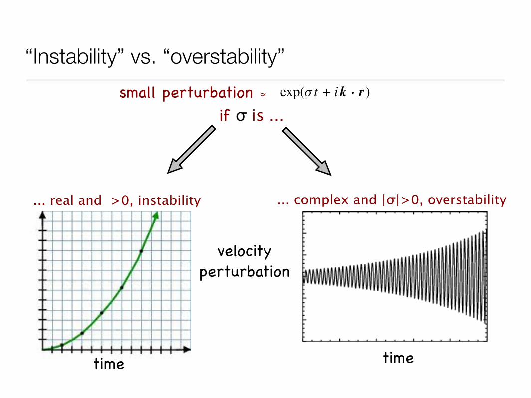
“Instability” vs. “overstability”

L98 BALBUS & REYNOLDS Vol. 720

gradient. We generalize the treatment of Q08 to include opti-cally thin radiative losses. Our principal result is the finding ofnew overstabilities of dynamical waves. More precisely, we findthat nominally stable configurations resulting from the nonlin-ear evolution of the HBI (i.e., temperature increasing upwardand magnetic field essentially horizontal) generate overstableg-modes via radiative losses. Nominally stable configurationsresulting from the nonlinear evolution of the MTI (i.e., tem-perature decreasing upward and magnetic field essentially ver-tical) generate overstable g-modes via anisotropic thermalconduction. In addition to furnishing a more complete for-mal picture of the stability properties of dilute plasma atmo-spheres, these findings may have significant implications forthe physical behavior of the ICM and should guide futuresimulations.

In the next section, we present the calculation in detail, andin the final section of this Letter, we conclude with a briefdiscussion of the implications of our findings.

2. ANALYSIS

We use the standard equations of MHD with the entropyequation augmented with anisotropic thermal conduction alongmagnetic field lines (Braginskii 1965) and radiative losses (e.g.,Field 1965). The mass, momentum, induction, and entropyequations are, respectively,

!"

!t+ !·("v) = 0, (1)

"Dv

Dt= (!!B)!B

4#" !P + "g, (2)

! B!t

= !!(v!B), (3)

D ln P""$

Dt= "$ " 1

P[!· Q + "L] , (4)

where " is the mass density, v is the fluid velocity, B is themagnetic field, g is the gravitational acceleration, P is the gaspressure, $ is the adiabatic index (5/3 for monotonic gas), Qis the heat flux, and L is the radiative energy loss per unit massof fluid, whose form we will leave unspecified. For thermalbremsstrahlung, a reasonable approximation is

"L # 2 $ 10"27n2eT

1/2 erg cm"3 s"1, (5)

where ne is the electron number density. D/Dt is the Lagrangianderivative, !/!t + v·!.

To define the heat flux Q, let b be a unit vector in the directionof the magnetic field. Then (Balbus 2001),

Q = "%b(b·!)T , (6)

where T is the kinetic gas temperature and % is the thermalconductivity (Spitzer 1982)

% # 6 $ 10"7T 5/2 erg cm"1 s"1 K"1. (7)

Finally, we follow Q08 and use the notation

& % %T/P (8)

for the thermal diffusion coefficient.

2.1. Equilibrium Background

We consider a gas stratified in the vertical z direction withtemperature profile T (z). The gas is not self-gravitating, sothat g is a specified function of position. We assume a highlysub-thermal magnetic field. Thus, in equilibrium, the gas is inhydrostatic balance,

dP

dz= ""g. (9)

The magnetic field is uniform with x and z components Bx andBz (in this way defining the x-axis), and unit vectors bx = Bx/B,bz = Bz/B. In equilibrium, there is a thermal balance betweenconductive heating and radiative losses,

" !· Q %d2

!b2

z%"T

dz2= "L. (10)

2.2. Local WKB Perturbations

As in Q08, we consider plane wave disturbances of theform exp(' t + ik · r) where the wavenumber k has Cartesiancomponents (kx, ky, kz) and r is the position vector. We differin notation from Q08 by using ' , a formal growth rate, ratherthan (, an angular frequency. This ensures that all coefficientsin the final dispersion relation are real. We work in the WKB(kr & 1) and Boussinesq limits (Q08).

We next consider the linearized equations when perturbations)", )v, etc., are applied to the equilibrium state. The heart ofthe problem is the entropy equation, so let us begin here. Thelinearized form of Equation (4) is

" $ ')"

"+ )vz

d ln P""$

dz= ($ " 1)

#"!·) Q

P" !T |P )T

$,

(11)where

! % "L/P, (12)

and

!T |P %#!!!T

$

P

, (13)

that is, the derivative of ! with respect to T with P held constant.We have used the Boussinesq approximation in ignoring allterms proportional to )P in Equation (11). In the process, wehave implicitly regarded ! as a function of T and P (rather thanthe more customary but less convenient T and " dependence).The remaining linearized equations,

k · )v = 0, (14)

')v = )"

"2

dP

dz" ik

%)P

"+

B·)B4#"

&+

i(k · B))B4#"

, (15)

')B = i(k · B))v, (16)

are, apart from notational convention, identical to Q08. Theentire system of equations differs from Q08 only by the ! term.The resulting dispersion relation is

%' +

$ " 1$

T !T |P + C&

(' 2 + (k · vA)2)

+'k2

'N2

k2+ CK

g

k2

d ln T

dz= 0, (17)

small perturbation ∝if σ is ...

... real and >0, instability ... complex and |σ|>0, overstability

time time

velocity perturbation

Stability criteria

thermal stability (Field criterion):

thermal/heat flux driven instabilities:

radiative cooling/heat flux driven overstabilities:

No. 1, 2010 RADIATIVE AND DYNAMIC STABILITY OF A DILUTE PLASMA L99

where

N2 = ! 1!"

dP

dz

d ln P!!"

dz= g

d ln P (1!" )/" T

dz, (18)

C =!

" ! 1"

"#(k·b)2, (19)

K =#1 ! 2b2

z

$k2" + 2bxbzkxkz. (20)

This corresponds to Equation (13) of Q08, except, as noted,for the single appearance of the radiative !T |P term. (A lessgeneral version of this result was also presented in Balbus& Reynolds 2008.) The dispersion characterizes the linearresponse of a magnetized, thermally conducting radiative diluteplasma to incompressible disturbances.

2.3. Stability

2.3.1. Recovery of the Conductive Field Criterion

Expanding the dispersion relation (17) leads to

$ 3 + a1$2 + a2$ + a3 = 0, (21)

where

a1 =!

" ! 1"

"T !T |P + C, (22)

a2 = k2"

k2N2 + (k · vA)2, (23)

a3 = CKg

k2

d ln T

dz+ (k · vA)2a1. (24)

There are stable solutions to this dispersion relation if andonly if the following three criteria are met:

a1 > 0, a3 > 0, a1a2 > a3. (25)

This follows from a Routh–Hurwitz analysis, but can be seenmore easily by inspection: the first two are in fact elementary,while the third follows from self-consistently demanding purelyimaginary solutions to the cubic equation and then investigatingtheir behavior for infinitesimal real parts.

The physical interpretation of a1 > 0, or

T !T |P + (k·b)2# > 0, (26)

is the magnetized conduction variation of the classical thermalinstability criterion (Field 1965). Only the component of k alongthe field lines enters into the conduction term.

2.3.2. Recovery of the HBI and MTI

We next consider the physical interpretation of a3 > 0, or

CKg

k2

d ln T

dz+ (k · vA)2a1 > 0. (27)

In essence, this is the HBI/MTI criterion of Q08, but further(de)stabilized when the flow is (un)stable by the isobaric Fieldcriterion. This is a true instability if a3 is negative, with$ = !a3/a2 in the limit of large a2 > 0.

Equation (27) shows that thermal instability and the HBI/MTI are intimately linked. To be definite, consider the behaviorof the HBI. The discussion of Q08 explains how the distortion

of field lines leads to conductive cooling of a downwardly dis-placed fluid element (and vice versa for an upwardly displacedelement). It is this cooling that causes the convection associ-ated with the HBI. With radiative losses present, the coolingis enhanced on a downward displacement, and relative heat-ing is present on an upward displacement. In fact, we mayimagine now slowly turning on the magnetic field from dy-namically weak to strongly dominant. Then, the exponentiallygrowing instability transforms from the Q08 HBI to the classi-cal (nonoscillatory) thermal instability. The role of the magneticfield in mediating this transition is crucial.

2.3.3. Destabilization of Wave Modes by a Positive Thermal Gradient

We now return to the third criterion, a1a2 > a3. With a3 > 0,this criterion is a more stringent stability criterion than the first(a1 > 0), and hence replaces it.

When a2 is large and positive (e.g., either N2 or (k · vA)2

is dominant), the unstable roots depending on a1 will beapproximately

$ = ±ia1/22 + (a3 ! a1a2)/2a2. (28)

On the other hand, at large wavenumbers, we may have a1and a3 as the dominant terms. If a3 and a1 are both positive (orboth negative), then the wavelike solutions will be

$ = ±i(a3/a1)1/2 + (a3 ! a1a2)/2a21 . (29)

In either case above, the combination a3 ! a1a2 determinesthe stability of the mode.

After a cancellation of the magnetic tension terms, thecondition a1a2 ! a3 > 0 becomes

a1k2"

k2N2 ! CK

g

k2

d ln T

dz> 0. (30)

Consider the limit bz # 1, which is HBI stable (a3 > 0)for all but nearly axial wavenumbers, whose growth times thenbecome very long. (We cannot take bz = 0 exactly, since thatwould preclude a static radiative equilibrium state. For bz finite,Equation (10) shows that the equilibrium dT /dz scales as b!1

z .)Then, K = k2

", and our inequality reduces to

" ! 1"

T !T |P N2 + C!

N2 ! gd ln T

dz

"> 0. (31)

But

N2 ! gd ln T

dz= " ! 1

"

1P!

!dP

dz

"2

, (32)

and assuming that N2 > 0, the inequality may be yet furtherreduced:

T !T |P +C

!PN2

!dP

dz

"2

> 0. (33)

Finally, substituting for C and N2 and simplifying, ourcondition becomes

T !T |P + #(k · b)2R > 0, (34)

where R is the reduction factor

R =!

1 +%%%%

"

" ! 1d ln T

d ln P

%%%%

"!1

, (35)

No. 1, 2010 RADIATIVE AND DYNAMIC STABILITY OF A DILUTE PLASMA L99

where

N2 = ! 1!"

dP

dz

d ln P!!"

dz= g

d ln P (1!" )/" T

dz, (18)

C =!

" ! 1"

"#(k·b)2, (19)

K =#1 ! 2b2

z

$k2" + 2bxbzkxkz. (20)

This corresponds to Equation (13) of Q08, except, as noted,for the single appearance of the radiative !T |P term. (A lessgeneral version of this result was also presented in Balbus& Reynolds 2008.) The dispersion characterizes the linearresponse of a magnetized, thermally conducting radiative diluteplasma to incompressible disturbances.

2.3. Stability

2.3.1. Recovery of the Conductive Field Criterion

Expanding the dispersion relation (17) leads to

$ 3 + a1$2 + a2$ + a3 = 0, (21)

where

a1 =!

" ! 1"

"T !T |P + C, (22)

a2 = k2"

k2N2 + (k · vA)2, (23)

a3 = CKg

k2

d ln T

dz+ (k · vA)2a1. (24)

There are stable solutions to this dispersion relation if andonly if the following three criteria are met:

a1 > 0, a3 > 0, a1a2 > a3. (25)

This follows from a Routh–Hurwitz analysis, but can be seenmore easily by inspection: the first two are in fact elementary,while the third follows from self-consistently demanding purelyimaginary solutions to the cubic equation and then investigatingtheir behavior for infinitesimal real parts.

The physical interpretation of a1 > 0, or

T !T |P + (k·b)2# > 0, (26)

is the magnetized conduction variation of the classical thermalinstability criterion (Field 1965). Only the component of k alongthe field lines enters into the conduction term.

2.3.2. Recovery of the HBI and MTI

We next consider the physical interpretation of a3 > 0, or

CKg

k2

d ln T

dz+ (k · vA)2a1 > 0. (27)

In essence, this is the HBI/MTI criterion of Q08, but further(de)stabilized when the flow is (un)stable by the isobaric Fieldcriterion. This is a true instability if a3 is negative, with$ = !a3/a2 in the limit of large a2 > 0.

Equation (27) shows that thermal instability and the HBI/MTI are intimately linked. To be definite, consider the behaviorof the HBI. The discussion of Q08 explains how the distortion

of field lines leads to conductive cooling of a downwardly dis-placed fluid element (and vice versa for an upwardly displacedelement). It is this cooling that causes the convection associ-ated with the HBI. With radiative losses present, the coolingis enhanced on a downward displacement, and relative heat-ing is present on an upward displacement. In fact, we mayimagine now slowly turning on the magnetic field from dy-namically weak to strongly dominant. Then, the exponentiallygrowing instability transforms from the Q08 HBI to the classi-cal (nonoscillatory) thermal instability. The role of the magneticfield in mediating this transition is crucial.

2.3.3. Destabilization of Wave Modes by a Positive Thermal Gradient

We now return to the third criterion, a1a2 > a3. With a3 > 0,this criterion is a more stringent stability criterion than the first(a1 > 0), and hence replaces it.

When a2 is large and positive (e.g., either N2 or (k · vA)2

is dominant), the unstable roots depending on a1 will beapproximately

$ = ±ia1/22 + (a3 ! a1a2)/2a2. (28)

On the other hand, at large wavenumbers, we may have a1and a3 as the dominant terms. If a3 and a1 are both positive (orboth negative), then the wavelike solutions will be

$ = ±i(a3/a1)1/2 + (a3 ! a1a2)/2a21 . (29)

In either case above, the combination a3 ! a1a2 determinesthe stability of the mode.

After a cancellation of the magnetic tension terms, thecondition a1a2 ! a3 > 0 becomes

a1k2"

k2N2 ! CK

g

k2

d ln T

dz> 0. (30)

Consider the limit bz # 1, which is HBI stable (a3 > 0)for all but nearly axial wavenumbers, whose growth times thenbecome very long. (We cannot take bz = 0 exactly, since thatwould preclude a static radiative equilibrium state. For bz finite,Equation (10) shows that the equilibrium dT /dz scales as b!1

z .)Then, K = k2

", and our inequality reduces to

" ! 1"

T !T |P N2 + C!

N2 ! gd ln T

dz

"> 0. (31)

But

N2 ! gd ln T

dz= " ! 1

"

1P!

!dP

dz

"2

, (32)

and assuming that N2 > 0, the inequality may be yet furtherreduced:

T !T |P +C

!PN2

!dP

dz

"2

> 0. (33)

Finally, substituting for C and N2 and simplifying, ourcondition becomes

T !T |P + #(k · b)2R > 0, (34)

where R is the reduction factor

R =!

1 +%%%%

"

" ! 1d ln T

d ln P

%%%%

"!1

, (35)

No. 1, 2010 RADIATIVE AND DYNAMIC STABILITY OF A DILUTE PLASMA L99

where

N2 = ! 1!"

dP

dz

d ln P!!"

dz= g

d ln P (1!" )/" T

dz, (18)

C =!

" ! 1"

"#(k·b)2, (19)

K =#1 ! 2b2

z

$k2" + 2bxbzkxkz. (20)

This corresponds to Equation (13) of Q08, except, as noted,for the single appearance of the radiative !T |P term. (A lessgeneral version of this result was also presented in Balbus& Reynolds 2008.) The dispersion characterizes the linearresponse of a magnetized, thermally conducting radiative diluteplasma to incompressible disturbances.

2.3. Stability

2.3.1. Recovery of the Conductive Field Criterion

Expanding the dispersion relation (17) leads to

$ 3 + a1$2 + a2$ + a3 = 0, (21)

where

a1 =!

" ! 1"

"T !T |P + C, (22)

a2 = k2"

k2N2 + (k · vA)2, (23)

a3 = CKg

k2

d ln T

dz+ (k · vA)2a1. (24)

There are stable solutions to this dispersion relation if andonly if the following three criteria are met:

a1 > 0, a3 > 0, a1a2 > a3. (25)

This follows from a Routh–Hurwitz analysis, but can be seenmore easily by inspection: the first two are in fact elementary,while the third follows from self-consistently demanding purelyimaginary solutions to the cubic equation and then investigatingtheir behavior for infinitesimal real parts.

The physical interpretation of a1 > 0, or

T !T |P + (k·b)2# > 0, (26)

is the magnetized conduction variation of the classical thermalinstability criterion (Field 1965). Only the component of k alongthe field lines enters into the conduction term.

2.3.2. Recovery of the HBI and MTI

We next consider the physical interpretation of a3 > 0, or

CKg

k2

d ln T

dz+ (k · vA)2a1 > 0. (27)

In essence, this is the HBI/MTI criterion of Q08, but further(de)stabilized when the flow is (un)stable by the isobaric Fieldcriterion. This is a true instability if a3 is negative, with$ = !a3/a2 in the limit of large a2 > 0.

Equation (27) shows that thermal instability and the HBI/MTI are intimately linked. To be definite, consider the behaviorof the HBI. The discussion of Q08 explains how the distortion

of field lines leads to conductive cooling of a downwardly dis-placed fluid element (and vice versa for an upwardly displacedelement). It is this cooling that causes the convection associ-ated with the HBI. With radiative losses present, the coolingis enhanced on a downward displacement, and relative heat-ing is present on an upward displacement. In fact, we mayimagine now slowly turning on the magnetic field from dy-namically weak to strongly dominant. Then, the exponentiallygrowing instability transforms from the Q08 HBI to the classi-cal (nonoscillatory) thermal instability. The role of the magneticfield in mediating this transition is crucial.

2.3.3. Destabilization of Wave Modes by a Positive Thermal Gradient

We now return to the third criterion, a1a2 > a3. With a3 > 0,this criterion is a more stringent stability criterion than the first(a1 > 0), and hence replaces it.

When a2 is large and positive (e.g., either N2 or (k · vA)2

is dominant), the unstable roots depending on a1 will beapproximately

$ = ±ia1/22 + (a3 ! a1a2)/2a2. (28)

On the other hand, at large wavenumbers, we may have a1and a3 as the dominant terms. If a3 and a1 are both positive (orboth negative), then the wavelike solutions will be

$ = ±i(a3/a1)1/2 + (a3 ! a1a2)/2a21 . (29)

In either case above, the combination a3 ! a1a2 determinesthe stability of the mode.

After a cancellation of the magnetic tension terms, thecondition a1a2 ! a3 > 0 becomes

a1k2"

k2N2 ! CK

g

k2

d ln T

dz> 0. (30)

Consider the limit bz # 1, which is HBI stable (a3 > 0)for all but nearly axial wavenumbers, whose growth times thenbecome very long. (We cannot take bz = 0 exactly, since thatwould preclude a static radiative equilibrium state. For bz finite,Equation (10) shows that the equilibrium dT /dz scales as b!1

z .)Then, K = k2

", and our inequality reduces to

" ! 1"

T !T |P N2 + C!

N2 ! gd ln T

dz

"> 0. (31)

But

N2 ! gd ln T

dz= " ! 1

"

1P!

!dP

dz

"2

, (32)

and assuming that N2 > 0, the inequality may be yet furtherreduced:

T !T |P +C

!PN2

!dP

dz

"2

> 0. (33)

Finally, substituting for C and N2 and simplifying, ourcondition becomes

T !T |P + #(k · b)2R > 0, (34)

where R is the reduction factor

R =!

1 +%%%%

"

" ! 1d ln T

d ln P

%%%%

"!1

, (35)

No. 1, 2010 RADIATIVE AND DYNAMIC STABILITY OF A DILUTE PLASMA L99

where

N2 = ! 1!"

dP

dz

d ln P!!"

dz= g

d ln P (1!" )/" T

dz, (18)

C =!

" ! 1"

"#(k·b)2, (19)

K =#1 ! 2b2

z

$k2" + 2bxbzkxkz. (20)

This corresponds to Equation (13) of Q08, except, as noted,for the single appearance of the radiative !T |P term. (A lessgeneral version of this result was also presented in Balbus& Reynolds 2008.) The dispersion characterizes the linearresponse of a magnetized, thermally conducting radiative diluteplasma to incompressible disturbances.

2.3. Stability

2.3.1. Recovery of the Conductive Field Criterion

Expanding the dispersion relation (17) leads to

$ 3 + a1$2 + a2$ + a3 = 0, (21)

where

a1 =!

" ! 1"

"T !T |P + C, (22)

a2 = k2"

k2N2 + (k · vA)2, (23)

a3 = CKg

k2

d ln T

dz+ (k · vA)2a1. (24)

There are stable solutions to this dispersion relation if andonly if the following three criteria are met:

a1 > 0, a3 > 0, a1a2 > a3. (25)

This follows from a Routh–Hurwitz analysis, but can be seenmore easily by inspection: the first two are in fact elementary,while the third follows from self-consistently demanding purelyimaginary solutions to the cubic equation and then investigatingtheir behavior for infinitesimal real parts.

The physical interpretation of a1 > 0, or

T !T |P + (k·b)2# > 0, (26)

is the magnetized conduction variation of the classical thermalinstability criterion (Field 1965). Only the component of k alongthe field lines enters into the conduction term.

2.3.2. Recovery of the HBI and MTI

We next consider the physical interpretation of a3 > 0, or

CKg

k2

d ln T

dz+ (k · vA)2a1 > 0. (27)

In essence, this is the HBI/MTI criterion of Q08, but further(de)stabilized when the flow is (un)stable by the isobaric Fieldcriterion. This is a true instability if a3 is negative, with$ = !a3/a2 in the limit of large a2 > 0.

Equation (27) shows that thermal instability and the HBI/MTI are intimately linked. To be definite, consider the behaviorof the HBI. The discussion of Q08 explains how the distortion

of field lines leads to conductive cooling of a downwardly dis-placed fluid element (and vice versa for an upwardly displacedelement). It is this cooling that causes the convection associ-ated with the HBI. With radiative losses present, the coolingis enhanced on a downward displacement, and relative heat-ing is present on an upward displacement. In fact, we mayimagine now slowly turning on the magnetic field from dy-namically weak to strongly dominant. Then, the exponentiallygrowing instability transforms from the Q08 HBI to the classi-cal (nonoscillatory) thermal instability. The role of the magneticfield in mediating this transition is crucial.

2.3.3. Destabilization of Wave Modes by a Positive Thermal Gradient

We now return to the third criterion, a1a2 > a3. With a3 > 0,this criterion is a more stringent stability criterion than the first(a1 > 0), and hence replaces it.

When a2 is large and positive (e.g., either N2 or (k · vA)2

is dominant), the unstable roots depending on a1 will beapproximately

$ = ±ia1/22 + (a3 ! a1a2)/2a2. (28)

On the other hand, at large wavenumbers, we may have a1and a3 as the dominant terms. If a3 and a1 are both positive (orboth negative), then the wavelike solutions will be

$ = ±i(a3/a1)1/2 + (a3 ! a1a2)/2a21 . (29)

In either case above, the combination a3 ! a1a2 determinesthe stability of the mode.

After a cancellation of the magnetic tension terms, thecondition a1a2 ! a3 > 0 becomes

a1k2"

k2N2 ! CK

g

k2

d ln T

dz> 0. (30)

Consider the limit bz # 1, which is HBI stable (a3 > 0)for all but nearly axial wavenumbers, whose growth times thenbecome very long. (We cannot take bz = 0 exactly, since thatwould preclude a static radiative equilibrium state. For bz finite,Equation (10) shows that the equilibrium dT /dz scales as b!1

z .)Then, K = k2

", and our inequality reduces to

" ! 1"

T !T |P N2 + C!

N2 ! gd ln T

dz

"> 0. (31)

But

N2 ! gd ln T

dz= " ! 1

"

1P!

!dP

dz

"2

, (32)

and assuming that N2 > 0, the inequality may be yet furtherreduced:

T !T |P +C

!PN2

!dP

dz

"2

> 0. (33)

Finally, substituting for C and N2 and simplifying, ourcondition becomes

T !T |P + #(k · b)2R > 0, (34)

where R is the reduction factor

R =!

1 +%%%%

"

" ! 1d ln T

d ln P

%%%%

"!1

, (35)

( )

No. 1, 2010 RADIATIVE AND DYNAMIC STABILITY OF A DILUTE PLASMA L99

where

N2 = ! 1!"

dP

dz

d ln P!!"

dz= g

d ln P (1!" )/" T

dz, (18)

C =!

" ! 1"

"#(k·b)2, (19)

K =#1 ! 2b2

z

$k2" + 2bxbzkxkz. (20)

This corresponds to Equation (13) of Q08, except, as noted,for the single appearance of the radiative !T |P term. (A lessgeneral version of this result was also presented in Balbus& Reynolds 2008.) The dispersion characterizes the linearresponse of a magnetized, thermally conducting radiative diluteplasma to incompressible disturbances.

2.3. Stability

2.3.1. Recovery of the Conductive Field Criterion

Expanding the dispersion relation (17) leads to

$ 3 + a1$2 + a2$ + a3 = 0, (21)

where

a1 =!

" ! 1"

"T !T |P + C, (22)

a2 = k2"

k2N2 + (k · vA)2, (23)

a3 = CKg

k2

d ln T

dz+ (k · vA)2a1. (24)

There are stable solutions to this dispersion relation if andonly if the following three criteria are met:

a1 > 0, a3 > 0, a1a2 > a3. (25)

This follows from a Routh–Hurwitz analysis, but can be seenmore easily by inspection: the first two are in fact elementary,while the third follows from self-consistently demanding purelyimaginary solutions to the cubic equation and then investigatingtheir behavior for infinitesimal real parts.

The physical interpretation of a1 > 0, or

T !T |P + (k·b)2# > 0, (26)

is the magnetized conduction variation of the classical thermalinstability criterion (Field 1965). Only the component of k alongthe field lines enters into the conduction term.

2.3.2. Recovery of the HBI and MTI

We next consider the physical interpretation of a3 > 0, or

CKg

k2

d ln T

dz+ (k · vA)2a1 > 0. (27)

In essence, this is the HBI/MTI criterion of Q08, but further(de)stabilized when the flow is (un)stable by the isobaric Fieldcriterion. This is a true instability if a3 is negative, with$ = !a3/a2 in the limit of large a2 > 0.

Equation (27) shows that thermal instability and the HBI/MTI are intimately linked. To be definite, consider the behaviorof the HBI. The discussion of Q08 explains how the distortion

of field lines leads to conductive cooling of a downwardly dis-placed fluid element (and vice versa for an upwardly displacedelement). It is this cooling that causes the convection associ-ated with the HBI. With radiative losses present, the coolingis enhanced on a downward displacement, and relative heat-ing is present on an upward displacement. In fact, we mayimagine now slowly turning on the magnetic field from dy-namically weak to strongly dominant. Then, the exponentiallygrowing instability transforms from the Q08 HBI to the classi-cal (nonoscillatory) thermal instability. The role of the magneticfield in mediating this transition is crucial.

2.3.3. Destabilization of Wave Modes by a Positive Thermal Gradient

We now return to the third criterion, a1a2 > a3. With a3 > 0,this criterion is a more stringent stability criterion than the first(a1 > 0), and hence replaces it.

When a2 is large and positive (e.g., either N2 or (k · vA)2

is dominant), the unstable roots depending on a1 will beapproximately

$ = ±ia1/22 + (a3 ! a1a2)/2a2. (28)

On the other hand, at large wavenumbers, we may have a1and a3 as the dominant terms. If a3 and a1 are both positive (orboth negative), then the wavelike solutions will be

$ = ±i(a3/a1)1/2 + (a3 ! a1a2)/2a21 . (29)

In either case above, the combination a3 ! a1a2 determinesthe stability of the mode.

After a cancellation of the magnetic tension terms, thecondition a1a2 ! a3 > 0 becomes

a1k2"

k2N2 ! CK

g

k2

d ln T

dz> 0. (30)

Consider the limit bz # 1, which is HBI stable (a3 > 0)for all but nearly axial wavenumbers, whose growth times thenbecome very long. (We cannot take bz = 0 exactly, since thatwould preclude a static radiative equilibrium state. For bz finite,Equation (10) shows that the equilibrium dT /dz scales as b!1

z .)Then, K = k2

", and our inequality reduces to

" ! 1"

T !T |P N2 + C!

N2 ! gd ln T

dz

"> 0. (31)

But

N2 ! gd ln T

dz= " ! 1

"

1P!

!dP

dz

"2

, (32)

and assuming that N2 > 0, the inequality may be yet furtherreduced:

T !T |P +C

!PN2

!dP

dz

"2

> 0. (33)

Finally, substituting for C and N2 and simplifying, ourcondition becomes

T !T |P + #(k · b)2R > 0, (34)

where R is the reduction factor

R =!

1 +%%%%

"

" ! 1d ln T

d ln P

%%%%

"!1

, (35)

No. 1, 2010 RADIATIVE AND DYNAMIC STABILITY OF A DILUTE PLASMA L99

where

N2 = ! 1!"

dP

dz

d ln P!!"

dz= g

d ln P (1!" )/" T

dz, (18)

C =!

" ! 1"

"#(k·b)2, (19)

K =#1 ! 2b2

z

$k2" + 2bxbzkxkz. (20)

This corresponds to Equation (13) of Q08, except, as noted,for the single appearance of the radiative !T |P term. (A lessgeneral version of this result was also presented in Balbus& Reynolds 2008.) The dispersion characterizes the linearresponse of a magnetized, thermally conducting radiative diluteplasma to incompressible disturbances.

2.3. Stability

2.3.1. Recovery of the Conductive Field Criterion

Expanding the dispersion relation (17) leads to

$ 3 + a1$2 + a2$ + a3 = 0, (21)

where

a1 =!

" ! 1"

"T !T |P + C, (22)

a2 = k2"

k2N2 + (k · vA)2, (23)

a3 = CKg

k2

d ln T

dz+ (k · vA)2a1. (24)

There are stable solutions to this dispersion relation if andonly if the following three criteria are met:

a1 > 0, a3 > 0, a1a2 > a3. (25)

This follows from a Routh–Hurwitz analysis, but can be seenmore easily by inspection: the first two are in fact elementary,while the third follows from self-consistently demanding purelyimaginary solutions to the cubic equation and then investigatingtheir behavior for infinitesimal real parts.

The physical interpretation of a1 > 0, or

T !T |P + (k·b)2# > 0, (26)

is the magnetized conduction variation of the classical thermalinstability criterion (Field 1965). Only the component of k alongthe field lines enters into the conduction term.

2.3.2. Recovery of the HBI and MTI

We next consider the physical interpretation of a3 > 0, or

CKg

k2

d ln T

dz+ (k · vA)2a1 > 0. (27)

In essence, this is the HBI/MTI criterion of Q08, but further(de)stabilized when the flow is (un)stable by the isobaric Fieldcriterion. This is a true instability if a3 is negative, with$ = !a3/a2 in the limit of large a2 > 0.

Equation (27) shows that thermal instability and the HBI/MTI are intimately linked. To be definite, consider the behaviorof the HBI. The discussion of Q08 explains how the distortion

of field lines leads to conductive cooling of a downwardly dis-placed fluid element (and vice versa for an upwardly displacedelement). It is this cooling that causes the convection associ-ated with the HBI. With radiative losses present, the coolingis enhanced on a downward displacement, and relative heat-ing is present on an upward displacement. In fact, we mayimagine now slowly turning on the magnetic field from dy-namically weak to strongly dominant. Then, the exponentiallygrowing instability transforms from the Q08 HBI to the classi-cal (nonoscillatory) thermal instability. The role of the magneticfield in mediating this transition is crucial.

2.3.3. Destabilization of Wave Modes by a Positive Thermal Gradient

We now return to the third criterion, a1a2 > a3. With a3 > 0,this criterion is a more stringent stability criterion than the first(a1 > 0), and hence replaces it.

When a2 is large and positive (e.g., either N2 or (k · vA)2

is dominant), the unstable roots depending on a1 will beapproximately

$ = ±ia1/22 + (a3 ! a1a2)/2a2. (28)

On the other hand, at large wavenumbers, we may have a1and a3 as the dominant terms. If a3 and a1 are both positive (orboth negative), then the wavelike solutions will be

$ = ±i(a3/a1)1/2 + (a3 ! a1a2)/2a21 . (29)

In either case above, the combination a3 ! a1a2 determinesthe stability of the mode.

After a cancellation of the magnetic tension terms, thecondition a1a2 ! a3 > 0 becomes

a1k2"

k2N2 ! CK

g

k2

d ln T

dz> 0. (30)

Consider the limit bz # 1, which is HBI stable (a3 > 0)for all but nearly axial wavenumbers, whose growth times thenbecome very long. (We cannot take bz = 0 exactly, since thatwould preclude a static radiative equilibrium state. For bz finite,Equation (10) shows that the equilibrium dT /dz scales as b!1

z .)Then, K = k2

", and our inequality reduces to

" ! 1"

T !T |P N2 + C!

N2 ! gd ln T

dz

"> 0. (31)

But

N2 ! gd ln T

dz= " ! 1

"

1P!

!dP

dz

"2

, (32)

and assuming that N2 > 0, the inequality may be yet furtherreduced:

T !T |P +C

!PN2

!dP

dz

"2

> 0. (33)

Finally, substituting for C and N2 and simplifying, ourcondition becomes

T !T |P + #(k · b)2R > 0, (34)

where R is the reduction factor

R =!

1 +%%%%

"

" ! 1d ln T

d ln P

%%%%

"!1

, (35)= f (dlnT, dlnp) < 1 “reduction factor”

L98 BALBUS & REYNOLDS Vol. 720

gradient. We generalize the treatment of Q08 to include opti-cally thin radiative losses. Our principal result is the finding ofnew overstabilities of dynamical waves. More precisely, we findthat nominally stable configurations resulting from the nonlin-ear evolution of the HBI (i.e., temperature increasing upwardand magnetic field essentially horizontal) generate overstableg-modes via radiative losses. Nominally stable configurationsresulting from the nonlinear evolution of the MTI (i.e., tem-perature decreasing upward and magnetic field essentially ver-tical) generate overstable g-modes via anisotropic thermalconduction. In addition to furnishing a more complete for-mal picture of the stability properties of dilute plasma atmo-spheres, these findings may have significant implications forthe physical behavior of the ICM and should guide futuresimulations.

In the next section, we present the calculation in detail, andin the final section of this Letter, we conclude with a briefdiscussion of the implications of our findings.

2. ANALYSIS

We use the standard equations of MHD with the entropyequation augmented with anisotropic thermal conduction alongmagnetic field lines (Braginskii 1965) and radiative losses (e.g.,Field 1965). The mass, momentum, induction, and entropyequations are, respectively,

!"

!t+ !·("v) = 0, (1)

"Dv

Dt= (!!B)!B

4#" !P + "g, (2)

! B!t

= !!(v!B), (3)

D ln P""$

Dt= "$ " 1

P[!· Q + "L] , (4)

where " is the mass density, v is the fluid velocity, B is themagnetic field, g is the gravitational acceleration, P is the gaspressure, $ is the adiabatic index (5/3 for monotonic gas), Qis the heat flux, and L is the radiative energy loss per unit massof fluid, whose form we will leave unspecified. For thermalbremsstrahlung, a reasonable approximation is

"L # 2 $ 10"27n2eT

1/2 erg cm"3 s"1, (5)

where ne is the electron number density. D/Dt is the Lagrangianderivative, !/!t + v·!.

To define the heat flux Q, let b be a unit vector in the directionof the magnetic field. Then (Balbus 2001),

Q = "%b(b·!)T , (6)

where T is the kinetic gas temperature and % is the thermalconductivity (Spitzer 1982)

% # 6 $ 10"7T 5/2 erg cm"1 s"1 K"1. (7)

Finally, we follow Q08 and use the notation

& % %T/P (8)

for the thermal diffusion coefficient.

2.1. Equilibrium Background

We consider a gas stratified in the vertical z direction withtemperature profile T (z). The gas is not self-gravitating, sothat g is a specified function of position. We assume a highlysub-thermal magnetic field. Thus, in equilibrium, the gas is inhydrostatic balance,

dP

dz= ""g. (9)

The magnetic field is uniform with x and z components Bx andBz (in this way defining the x-axis), and unit vectors bx = Bx/B,bz = Bz/B. In equilibrium, there is a thermal balance betweenconductive heating and radiative losses,

" !· Q %d2

!b2

z%"T

dz2= "L. (10)

2.2. Local WKB Perturbations

As in Q08, we consider plane wave disturbances of theform exp(' t + ik · r) where the wavenumber k has Cartesiancomponents (kx, ky, kz) and r is the position vector. We differin notation from Q08 by using ' , a formal growth rate, ratherthan (, an angular frequency. This ensures that all coefficientsin the final dispersion relation are real. We work in the WKB(kr & 1) and Boussinesq limits (Q08).

We next consider the linearized equations when perturbations)", )v, etc., are applied to the equilibrium state. The heart ofthe problem is the entropy equation, so let us begin here. Thelinearized form of Equation (4) is

" $ ')"

"+ )vz

d ln P""$

dz= ($ " 1)

#"!·) Q

P" !T |P )T

$,

(11)where

! % "L/P, (12)

and

!T |P %#!!!T

$

P

, (13)

that is, the derivative of ! with respect to T with P held constant.We have used the Boussinesq approximation in ignoring allterms proportional to )P in Equation (11). In the process, wehave implicitly regarded ! as a function of T and P (rather thanthe more customary but less convenient T and " dependence).The remaining linearized equations,

k · )v = 0, (14)

')v = )"

"2

dP

dz" ik

%)P

"+

B·)B4#"

&+

i(k · B))B4#"

, (15)

')B = i(k · B))v, (16)

are, apart from notational convention, identical to Q08. Theentire system of equations differs from Q08 only by the ! term.The resulting dispersion relation is

%' +

$ " 1$

T !T |P + C&

(' 2 + (k · vA)2)

+'k2

'N2

k2+ CK

g

k2

d ln T

dz= 0, (17)diffusivity (cm2/s) in terms

of Spitzer conductivity

No. 1, 2010 RADIATIVE AND DYNAMIC STABILITY OF A DILUTE PLASMA L99

where

N2 = ! 1!"

dP

dz

d ln P!!"

dz= g

d ln P (1!" )/" T

dz, (18)

C =!

" ! 1"

"#(k·b)2, (19)

K =#1 ! 2b2

z

$k2" + 2bxbzkxkz. (20)

This corresponds to Equation (13) of Q08, except, as noted,for the single appearance of the radiative !T |P term. (A lessgeneral version of this result was also presented in Balbus& Reynolds 2008.) The dispersion characterizes the linearresponse of a magnetized, thermally conducting radiative diluteplasma to incompressible disturbances.

2.3. Stability

2.3.1. Recovery of the Conductive Field Criterion

Expanding the dispersion relation (17) leads to

$ 3 + a1$2 + a2$ + a3 = 0, (21)

where

a1 =!

" ! 1"

"T !T |P + C, (22)

a2 = k2"

k2N2 + (k · vA)2, (23)

a3 = CKg

k2

d ln T

dz+ (k · vA)2a1. (24)

There are stable solutions to this dispersion relation if andonly if the following three criteria are met:

a1 > 0, a3 > 0, a1a2 > a3. (25)

This follows from a Routh–Hurwitz analysis, but can be seenmore easily by inspection: the first two are in fact elementary,while the third follows from self-consistently demanding purelyimaginary solutions to the cubic equation and then investigatingtheir behavior for infinitesimal real parts.

The physical interpretation of a1 > 0, or

T !T |P + (k·b)2# > 0, (26)

is the magnetized conduction variation of the classical thermalinstability criterion (Field 1965). Only the component of k alongthe field lines enters into the conduction term.

2.3.2. Recovery of the HBI and MTI

We next consider the physical interpretation of a3 > 0, or

CKg

k2

d ln T

dz+ (k · vA)2a1 > 0. (27)

In essence, this is the HBI/MTI criterion of Q08, but further(de)stabilized when the flow is (un)stable by the isobaric Fieldcriterion. This is a true instability if a3 is negative, with$ = !a3/a2 in the limit of large a2 > 0.

Equation (27) shows that thermal instability and the HBI/MTI are intimately linked. To be definite, consider the behaviorof the HBI. The discussion of Q08 explains how the distortion

of field lines leads to conductive cooling of a downwardly dis-placed fluid element (and vice versa for an upwardly displacedelement). It is this cooling that causes the convection associ-ated with the HBI. With radiative losses present, the coolingis enhanced on a downward displacement, and relative heat-ing is present on an upward displacement. In fact, we mayimagine now slowly turning on the magnetic field from dy-namically weak to strongly dominant. Then, the exponentiallygrowing instability transforms from the Q08 HBI to the classi-cal (nonoscillatory) thermal instability. The role of the magneticfield in mediating this transition is crucial.

2.3.3. Destabilization of Wave Modes by a Positive Thermal Gradient

We now return to the third criterion, a1a2 > a3. With a3 > 0,this criterion is a more stringent stability criterion than the first(a1 > 0), and hence replaces it.

When a2 is large and positive (e.g., either N2 or (k · vA)2

is dominant), the unstable roots depending on a1 will beapproximately

$ = ±ia1/22 + (a3 ! a1a2)/2a2. (28)

On the other hand, at large wavenumbers, we may have a1and a3 as the dominant terms. If a3 and a1 are both positive (orboth negative), then the wavelike solutions will be

$ = ±i(a3/a1)1/2 + (a3 ! a1a2)/2a21 . (29)

In either case above, the combination a3 ! a1a2 determinesthe stability of the mode.

After a cancellation of the magnetic tension terms, thecondition a1a2 ! a3 > 0 becomes

a1k2"

k2N2 ! CK

g

k2

d ln T

dz> 0. (30)

Consider the limit bz # 1, which is HBI stable (a3 > 0)for all but nearly axial wavenumbers, whose growth times thenbecome very long. (We cannot take bz = 0 exactly, since thatwould preclude a static radiative equilibrium state. For bz finite,Equation (10) shows that the equilibrium dT /dz scales as b!1

z .)Then, K = k2

", and our inequality reduces to

" ! 1"

T !T |P N2 + C!

N2 ! gd ln T

dz

"> 0. (31)

But

N2 ! gd ln T

dz= " ! 1

"

1P!

!dP

dz

"2

, (32)

and assuming that N2 > 0, the inequality may be yet furtherreduced:

T !T |P +C

!PN2

!dP

dz

"2

> 0. (33)

Finally, substituting for C and N2 and simplifying, ourcondition becomes

T !T |P + #(k · b)2R > 0, (34)

where R is the reduction factor

R =!

1 +%%%%

"

" ! 1d ln T

d ln P

%%%%

"!1

, (35)

No. 1, 2010 RADIATIVE AND DYNAMIC STABILITY OF A DILUTE PLASMA L99

where

N2 = ! 1!"

dP

dz

d ln P!!"

dz= g

d ln P (1!" )/" T

dz, (18)

C =!

" ! 1"

"#(k·b)2, (19)

K =#1 ! 2b2

z

$k2" + 2bxbzkxkz. (20)

This corresponds to Equation (13) of Q08, except, as noted,for the single appearance of the radiative !T |P term. (A lessgeneral version of this result was also presented in Balbus& Reynolds 2008.) The dispersion characterizes the linearresponse of a magnetized, thermally conducting radiative diluteplasma to incompressible disturbances.

2.3. Stability

2.3.1. Recovery of the Conductive Field Criterion

Expanding the dispersion relation (17) leads to

$ 3 + a1$2 + a2$ + a3 = 0, (21)

where

a1 =!

" ! 1"

"T !T |P + C, (22)

a2 = k2"

k2N2 + (k · vA)2, (23)

a3 = CKg

k2

d ln T

dz+ (k · vA)2a1. (24)

There are stable solutions to this dispersion relation if andonly if the following three criteria are met:

a1 > 0, a3 > 0, a1a2 > a3. (25)

This follows from a Routh–Hurwitz analysis, but can be seenmore easily by inspection: the first two are in fact elementary,while the third follows from self-consistently demanding purelyimaginary solutions to the cubic equation and then investigatingtheir behavior for infinitesimal real parts.

The physical interpretation of a1 > 0, or

T !T |P + (k·b)2# > 0, (26)

is the magnetized conduction variation of the classical thermalinstability criterion (Field 1965). Only the component of k alongthe field lines enters into the conduction term.

2.3.2. Recovery of the HBI and MTI

We next consider the physical interpretation of a3 > 0, or

CKg

k2

d ln T

dz+ (k · vA)2a1 > 0. (27)

In essence, this is the HBI/MTI criterion of Q08, but further(de)stabilized when the flow is (un)stable by the isobaric Fieldcriterion. This is a true instability if a3 is negative, with$ = !a3/a2 in the limit of large a2 > 0.

Equation (27) shows that thermal instability and the HBI/MTI are intimately linked. To be definite, consider the behaviorof the HBI. The discussion of Q08 explains how the distortion

of field lines leads to conductive cooling of a downwardly dis-placed fluid element (and vice versa for an upwardly displacedelement). It is this cooling that causes the convection associ-ated with the HBI. With radiative losses present, the coolingis enhanced on a downward displacement, and relative heat-ing is present on an upward displacement. In fact, we mayimagine now slowly turning on the magnetic field from dy-namically weak to strongly dominant. Then, the exponentiallygrowing instability transforms from the Q08 HBI to the classi-cal (nonoscillatory) thermal instability. The role of the magneticfield in mediating this transition is crucial.

2.3.3. Destabilization of Wave Modes by a Positive Thermal Gradient

We now return to the third criterion, a1a2 > a3. With a3 > 0,this criterion is a more stringent stability criterion than the first(a1 > 0), and hence replaces it.

When a2 is large and positive (e.g., either N2 or (k · vA)2

is dominant), the unstable roots depending on a1 will beapproximately

$ = ±ia1/22 + (a3 ! a1a2)/2a2. (28)

On the other hand, at large wavenumbers, we may have a1and a3 as the dominant terms. If a3 and a1 are both positive (orboth negative), then the wavelike solutions will be

$ = ±i(a3/a1)1/2 + (a3 ! a1a2)/2a21 . (29)

In either case above, the combination a3 ! a1a2 determinesthe stability of the mode.

After a cancellation of the magnetic tension terms, thecondition a1a2 ! a3 > 0 becomes

a1k2"

k2N2 ! CK

g

k2

d ln T

dz> 0. (30)

Consider the limit bz # 1, which is HBI stable (a3 > 0)for all but nearly axial wavenumbers, whose growth times thenbecome very long. (We cannot take bz = 0 exactly, since thatwould preclude a static radiative equilibrium state. For bz finite,Equation (10) shows that the equilibrium dT /dz scales as b!1

z .)Then, K = k2

", and our inequality reduces to

" ! 1"

T !T |P N2 + C!

N2 ! gd ln T

dz

"> 0. (31)

But

N2 ! gd ln T

dz= " ! 1

"

1P!

!dP

dz

"2

, (32)

and assuming that N2 > 0, the inequality may be yet furtherreduced:

T !T |P +C

!PN2

!dP

dz

"2

> 0. (33)

Finally, substituting for C and N2 and simplifying, ourcondition becomes

T !T |P + #(k · b)2R > 0, (34)

where R is the reduction factor

R =!

1 +%%%%

"

" ! 1d ln T

d ln P

%%%%

"!1

, (35)

No. 1, 2010 RADIATIVE AND DYNAMIC STABILITY OF A DILUTE PLASMA L99

where

N2 = ! 1!"

dP

dz

d ln P!!"

dz= g

d ln P (1!" )/" T

dz, (18)

C =!

" ! 1"

"#(k·b)2, (19)

K =#1 ! 2b2

z

$k2" + 2bxbzkxkz. (20)

This corresponds to Equation (13) of Q08, except, as noted,for the single appearance of the radiative !T |P term. (A lessgeneral version of this result was also presented in Balbus& Reynolds 2008.) The dispersion characterizes the linearresponse of a magnetized, thermally conducting radiative diluteplasma to incompressible disturbances.

2.3. Stability

2.3.1. Recovery of the Conductive Field Criterion

Expanding the dispersion relation (17) leads to

$ 3 + a1$2 + a2$ + a3 = 0, (21)

where

a1 =!

" ! 1"

"T !T |P + C, (22)

a2 = k2"

k2N2 + (k · vA)2, (23)

a3 = CKg

k2

d ln T

dz+ (k · vA)2a1. (24)

There are stable solutions to this dispersion relation if andonly if the following three criteria are met:

a1 > 0, a3 > 0, a1a2 > a3. (25)

This follows from a Routh–Hurwitz analysis, but can be seenmore easily by inspection: the first two are in fact elementary,while the third follows from self-consistently demanding purelyimaginary solutions to the cubic equation and then investigatingtheir behavior for infinitesimal real parts.

The physical interpretation of a1 > 0, or

T !T |P + (k·b)2# > 0, (26)

is the magnetized conduction variation of the classical thermalinstability criterion (Field 1965). Only the component of k alongthe field lines enters into the conduction term.

2.3.2. Recovery of the HBI and MTI

We next consider the physical interpretation of a3 > 0, or

CKg

k2

d ln T

dz+ (k · vA)2a1 > 0. (27)

In essence, this is the HBI/MTI criterion of Q08, but further(de)stabilized when the flow is (un)stable by the isobaric Fieldcriterion. This is a true instability if a3 is negative, with$ = !a3/a2 in the limit of large a2 > 0.

Equation (27) shows that thermal instability and the HBI/MTI are intimately linked. To be definite, consider the behaviorof the HBI. The discussion of Q08 explains how the distortion

of field lines leads to conductive cooling of a downwardly dis-placed fluid element (and vice versa for an upwardly displacedelement). It is this cooling that causes the convection associ-ated with the HBI. With radiative losses present, the coolingis enhanced on a downward displacement, and relative heat-ing is present on an upward displacement. In fact, we mayimagine now slowly turning on the magnetic field from dy-namically weak to strongly dominant. Then, the exponentiallygrowing instability transforms from the Q08 HBI to the classi-cal (nonoscillatory) thermal instability. The role of the magneticfield in mediating this transition is crucial.

2.3.3. Destabilization of Wave Modes by a Positive Thermal Gradient

We now return to the third criterion, a1a2 > a3. With a3 > 0,this criterion is a more stringent stability criterion than the first(a1 > 0), and hence replaces it.

When a2 is large and positive (e.g., either N2 or (k · vA)2

is dominant), the unstable roots depending on a1 will beapproximately

$ = ±ia1/22 + (a3 ! a1a2)/2a2. (28)

On the other hand, at large wavenumbers, we may have a1and a3 as the dominant terms. If a3 and a1 are both positive (orboth negative), then the wavelike solutions will be

$ = ±i(a3/a1)1/2 + (a3 ! a1a2)/2a21 . (29)

In either case above, the combination a3 ! a1a2 determinesthe stability of the mode.

After a cancellation of the magnetic tension terms, thecondition a1a2 ! a3 > 0 becomes

a1k2"

k2N2 ! CK

g

k2

d ln T

dz> 0. (30)

Consider the limit bz # 1, which is HBI stable (a3 > 0)for all but nearly axial wavenumbers, whose growth times thenbecome very long. (We cannot take bz = 0 exactly, since thatwould preclude a static radiative equilibrium state. For bz finite,Equation (10) shows that the equilibrium dT /dz scales as b!1

z .)Then, K = k2

", and our inequality reduces to

" ! 1"

T !T |P N2 + C!

N2 ! gd ln T

dz

"> 0. (31)

But

N2 ! gd ln T

dz= " ! 1

"

1P!

!dP

dz

"2

, (32)

and assuming that N2 > 0, the inequality may be yet furtherreduced:

T !T |P +C

!PN2

!dP

dz

"2

> 0. (33)

Finally, substituting for C and N2 and simplifying, ourcondition becomes

T !T |P + #(k · b)2R > 0, (34)

where R is the reduction factor

R =!

1 +%%%%

"

" ! 1d ln T

d ln P

%%%%

"!1

, (35)

No. 1, 2010 RADIATIVE AND DYNAMIC STABILITY OF A DILUTE PLASMA L99

where

N2 = ! 1!"

dP

dz

d ln P!!"

dz= g

d ln P (1!" )/" T

dz, (18)

C =!

" ! 1"

"#(k·b)2, (19)

K =#1 ! 2b2

z

$k2" + 2bxbzkxkz. (20)

This corresponds to Equation (13) of Q08, except, as noted,for the single appearance of the radiative !T |P term. (A lessgeneral version of this result was also presented in Balbus& Reynolds 2008.) The dispersion characterizes the linearresponse of a magnetized, thermally conducting radiative diluteplasma to incompressible disturbances.

2.3. Stability

2.3.1. Recovery of the Conductive Field Criterion

Expanding the dispersion relation (17) leads to

$ 3 + a1$2 + a2$ + a3 = 0, (21)

where

a1 =!

" ! 1"

"T !T |P + C, (22)

a2 = k2"

k2N2 + (k · vA)2, (23)

a3 = CKg

k2

d ln T

dz+ (k · vA)2a1. (24)

There are stable solutions to this dispersion relation if andonly if the following three criteria are met:

a1 > 0, a3 > 0, a1a2 > a3. (25)

This follows from a Routh–Hurwitz analysis, but can be seenmore easily by inspection: the first two are in fact elementary,while the third follows from self-consistently demanding purelyimaginary solutions to the cubic equation and then investigatingtheir behavior for infinitesimal real parts.

The physical interpretation of a1 > 0, or

T !T |P + (k·b)2# > 0, (26)

is the magnetized conduction variation of the classical thermalinstability criterion (Field 1965). Only the component of k alongthe field lines enters into the conduction term.

2.3.2. Recovery of the HBI and MTI

We next consider the physical interpretation of a3 > 0, or

CKg

k2

d ln T

dz+ (k · vA)2a1 > 0. (27)

In essence, this is the HBI/MTI criterion of Q08, but further(de)stabilized when the flow is (un)stable by the isobaric Fieldcriterion. This is a true instability if a3 is negative, with$ = !a3/a2 in the limit of large a2 > 0.

Equation (27) shows that thermal instability and the HBI/MTI are intimately linked. To be definite, consider the behaviorof the HBI. The discussion of Q08 explains how the distortion

of field lines leads to conductive cooling of a downwardly dis-placed fluid element (and vice versa for an upwardly displacedelement). It is this cooling that causes the convection associ-ated with the HBI. With radiative losses present, the coolingis enhanced on a downward displacement, and relative heat-ing is present on an upward displacement. In fact, we mayimagine now slowly turning on the magnetic field from dy-namically weak to strongly dominant. Then, the exponentiallygrowing instability transforms from the Q08 HBI to the classi-cal (nonoscillatory) thermal instability. The role of the magneticfield in mediating this transition is crucial.

2.3.3. Destabilization of Wave Modes by a Positive Thermal Gradient

We now return to the third criterion, a1a2 > a3. With a3 > 0,this criterion is a more stringent stability criterion than the first(a1 > 0), and hence replaces it.

When a2 is large and positive (e.g., either N2 or (k · vA)2

is dominant), the unstable roots depending on a1 will beapproximately

$ = ±ia1/22 + (a3 ! a1a2)/2a2. (28)

On the other hand, at large wavenumbers, we may have a1and a3 as the dominant terms. If a3 and a1 are both positive (orboth negative), then the wavelike solutions will be

$ = ±i(a3/a1)1/2 + (a3 ! a1a2)/2a21 . (29)

In either case above, the combination a3 ! a1a2 determinesthe stability of the mode.

After a cancellation of the magnetic tension terms, thecondition a1a2 ! a3 > 0 becomes

a1k2"

k2N2 ! CK

g

k2

d ln T

dz> 0. (30)

Consider the limit bz # 1, which is HBI stable (a3 > 0)for all but nearly axial wavenumbers, whose growth times thenbecome very long. (We cannot take bz = 0 exactly, since thatwould preclude a static radiative equilibrium state. For bz finite,Equation (10) shows that the equilibrium dT /dz scales as b!1

z .)Then, K = k2

", and our inequality reduces to

" ! 1"

T !T |P N2 + C!

N2 ! gd ln T

dz

"> 0. (31)

But

N2 ! gd ln T

dz= " ! 1

"

1P!

!dP

dz

"2

, (32)

and assuming that N2 > 0, the inequality may be yet furtherreduced:

T !T |P +C

!PN2

!dP

dz

"2

> 0. (33)

Finally, substituting for C and N2 and simplifying, ourcondition becomes

T !T |P + #(k · b)2R > 0, (34)

where R is the reduction factor

R =!

1 +%%%%

"

" ! 1d ln T

d ln P

%%%%

"!1

, (35)

No. 1, 2010 RADIATIVE AND DYNAMIC STABILITY OF A DILUTE PLASMA L99

where

N2 = ! 1!"

dP

dz

d ln P!!"

dz= g

d ln P (1!" )/" T

dz, (18)

C =!

" ! 1"

"#(k·b)2, (19)

K =#1 ! 2b2

z

$k2" + 2bxbzkxkz. (20)

This corresponds to Equation (13) of Q08, except, as noted,for the single appearance of the radiative !T |P term. (A lessgeneral version of this result was also presented in Balbus& Reynolds 2008.) The dispersion characterizes the linearresponse of a magnetized, thermally conducting radiative diluteplasma to incompressible disturbances.

2.3. Stability

2.3.1. Recovery of the Conductive Field Criterion

Expanding the dispersion relation (17) leads to

$ 3 + a1$2 + a2$ + a3 = 0, (21)

where

a1 =!

" ! 1"

"T !T |P + C, (22)

a2 = k2"

k2N2 + (k · vA)2, (23)

a3 = CKg

k2

d ln T

dz+ (k · vA)2a1. (24)

There are stable solutions to this dispersion relation if andonly if the following three criteria are met:

a1 > 0, a3 > 0, a1a2 > a3. (25)

This follows from a Routh–Hurwitz analysis, but can be seenmore easily by inspection: the first two are in fact elementary,while the third follows from self-consistently demanding purelyimaginary solutions to the cubic equation and then investigatingtheir behavior for infinitesimal real parts.

The physical interpretation of a1 > 0, or

T !T |P + (k·b)2# > 0, (26)

is the magnetized conduction variation of the classical thermalinstability criterion (Field 1965). Only the component of k alongthe field lines enters into the conduction term.

2.3.2. Recovery of the HBI and MTI

We next consider the physical interpretation of a3 > 0, or

CKg

k2

d ln T

dz+ (k · vA)2a1 > 0. (27)

In essence, this is the HBI/MTI criterion of Q08, but further(de)stabilized when the flow is (un)stable by the isobaric Fieldcriterion. This is a true instability if a3 is negative, with$ = !a3/a2 in the limit of large a2 > 0.

Equation (27) shows that thermal instability and the HBI/MTI are intimately linked. To be definite, consider the behaviorof the HBI. The discussion of Q08 explains how the distortion

of field lines leads to conductive cooling of a downwardly dis-placed fluid element (and vice versa for an upwardly displacedelement). It is this cooling that causes the convection associ-ated with the HBI. With radiative losses present, the coolingis enhanced on a downward displacement, and relative heat-ing is present on an upward displacement. In fact, we mayimagine now slowly turning on the magnetic field from dy-namically weak to strongly dominant. Then, the exponentiallygrowing instability transforms from the Q08 HBI to the classi-cal (nonoscillatory) thermal instability. The role of the magneticfield in mediating this transition is crucial.

2.3.3. Destabilization of Wave Modes by a Positive Thermal Gradient

We now return to the third criterion, a1a2 > a3. With a3 > 0,this criterion is a more stringent stability criterion than the first(a1 > 0), and hence replaces it.

When a2 is large and positive (e.g., either N2 or (k · vA)2

is dominant), the unstable roots depending on a1 will beapproximately

$ = ±ia1/22 + (a3 ! a1a2)/2a2. (28)

On the other hand, at large wavenumbers, we may have a1and a3 as the dominant terms. If a3 and a1 are both positive (orboth negative), then the wavelike solutions will be

$ = ±i(a3/a1)1/2 + (a3 ! a1a2)/2a21 . (29)

In either case above, the combination a3 ! a1a2 determinesthe stability of the mode.

After a cancellation of the magnetic tension terms, thecondition a1a2 ! a3 > 0 becomes

a1k2"

k2N2 ! CK

g

k2

d ln T

dz> 0. (30)

Consider the limit bz # 1, which is HBI stable (a3 > 0)for all but nearly axial wavenumbers, whose growth times thenbecome very long. (We cannot take bz = 0 exactly, since thatwould preclude a static radiative equilibrium state. For bz finite,Equation (10) shows that the equilibrium dT /dz scales as b!1

z .)Then, K = k2

", and our inequality reduces to

" ! 1"

T !T |P N2 + C!

N2 ! gd ln T

dz

"> 0. (31)

But

N2 ! gd ln T

dz= " ! 1

"

1P!

!dP

dz

"2

, (32)

and assuming that N2 > 0, the inequality may be yet furtherreduced:

T !T |P +C

!PN2

!dP

dz

"2

> 0. (33)

Finally, substituting for C and N2 and simplifying, ourcondition becomes

T !T |P + #(k · b)2R > 0, (34)

where R is the reduction factor

R =!

1 +%%%%

"

" ! 1d ln T

d ln P

%%%%

"!1

, (35)

<

No. 1, 2010 RADIATIVE AND DYNAMIC STABILITY OF A DILUTE PLASMA L99

where

N2 = ! 1!"

dP

dz

d ln P!!"

dz= g

d ln P (1!" )/" T

dz, (18)

C =!

" ! 1"

"#(k·b)2, (19)

K =#1 ! 2b2

z

$k2" + 2bxbzkxkz. (20)

This corresponds to Equation (13) of Q08, except, as noted,for the single appearance of the radiative !T |P term. (A lessgeneral version of this result was also presented in Balbus& Reynolds 2008.) The dispersion characterizes the linearresponse of a magnetized, thermally conducting radiative diluteplasma to incompressible disturbances.

2.3. Stability

2.3.1. Recovery of the Conductive Field Criterion

Expanding the dispersion relation (17) leads to

$ 3 + a1$2 + a2$ + a3 = 0, (21)

where

a1 =!

" ! 1"

"T !T |P + C, (22)

a2 = k2"

k2N2 + (k · vA)2, (23)

a3 = CKg

k2

d ln T

dz+ (k · vA)2a1. (24)

There are stable solutions to this dispersion relation if andonly if the following three criteria are met:

a1 > 0, a3 > 0, a1a2 > a3. (25)

This follows from a Routh–Hurwitz analysis, but can be seenmore easily by inspection: the first two are in fact elementary,while the third follows from self-consistently demanding purelyimaginary solutions to the cubic equation and then investigatingtheir behavior for infinitesimal real parts.

The physical interpretation of a1 > 0, or

T !T |P + (k·b)2# > 0, (26)

is the magnetized conduction variation of the classical thermalinstability criterion (Field 1965). Only the component of k alongthe field lines enters into the conduction term.

2.3.2. Recovery of the HBI and MTI

We next consider the physical interpretation of a3 > 0, or

CKg

k2

d ln T

dz+ (k · vA)2a1 > 0. (27)

In essence, this is the HBI/MTI criterion of Q08, but further(de)stabilized when the flow is (un)stable by the isobaric Fieldcriterion. This is a true instability if a3 is negative, with$ = !a3/a2 in the limit of large a2 > 0.

Equation (27) shows that thermal instability and the HBI/MTI are intimately linked. To be definite, consider the behaviorof the HBI. The discussion of Q08 explains how the distortion

of field lines leads to conductive cooling of a downwardly dis-placed fluid element (and vice versa for an upwardly displacedelement). It is this cooling that causes the convection associ-ated with the HBI. With radiative losses present, the coolingis enhanced on a downward displacement, and relative heat-ing is present on an upward displacement. In fact, we mayimagine now slowly turning on the magnetic field from dy-namically weak to strongly dominant. Then, the exponentiallygrowing instability transforms from the Q08 HBI to the classi-cal (nonoscillatory) thermal instability. The role of the magneticfield in mediating this transition is crucial.

2.3.3. Destabilization of Wave Modes by a Positive Thermal Gradient

We now return to the third criterion, a1a2 > a3. With a3 > 0,this criterion is a more stringent stability criterion than the first(a1 > 0), and hence replaces it.

When a2 is large and positive (e.g., either N2 or (k · vA)2

is dominant), the unstable roots depending on a1 will beapproximately

$ = ±ia1/22 + (a3 ! a1a2)/2a2. (28)

On the other hand, at large wavenumbers, we may have a1and a3 as the dominant terms. If a3 and a1 are both positive (orboth negative), then the wavelike solutions will be

$ = ±i(a3/a1)1/2 + (a3 ! a1a2)/2a21 . (29)

In either case above, the combination a3 ! a1a2 determinesthe stability of the mode.

After a cancellation of the magnetic tension terms, thecondition a1a2 ! a3 > 0 becomes

a1k2"

k2N2 ! CK

g

k2

d ln T

dz> 0. (30)

Consider the limit bz # 1, which is HBI stable (a3 > 0)for all but nearly axial wavenumbers, whose growth times thenbecome very long. (We cannot take bz = 0 exactly, since thatwould preclude a static radiative equilibrium state. For bz finite,Equation (10) shows that the equilibrium dT /dz scales as b!1

z .)Then, K = k2

", and our inequality reduces to

" ! 1"

T !T |P N2 + C!

N2 ! gd ln T

dz

"> 0. (31)

But

N2 ! gd ln T

dz= " ! 1

"

1P!

!dP

dz

"2

, (32)

and assuming that N2 > 0, the inequality may be yet furtherreduced:

T !T |P +C

!PN2

!dP

dz

"2

> 0. (33)

Finally, substituting for C and N2 and simplifying, ourcondition becomes

T !T |P + #(k · b)2R > 0, (34)

where R is the reduction factor

R =!

1 +%%%%

"

" ! 1d ln T

d ln P

%%%%

"!1

, (35)

<

No. 1, 2010 RADIATIVE AND DYNAMIC STABILITY OF A DILUTE PLASMA L99

where

N2 = ! 1!"

dP

dz

d ln P!!"

dz= g

d ln P (1!" )/" T

dz, (18)

C =!

" ! 1"

"#(k·b)2, (19)

K =#1 ! 2b2

z

$k2" + 2bxbzkxkz. (20)

This corresponds to Equation (13) of Q08, except, as noted,for the single appearance of the radiative !T |P term. (A lessgeneral version of this result was also presented in Balbus& Reynolds 2008.) The dispersion characterizes the linearresponse of a magnetized, thermally conducting radiative diluteplasma to incompressible disturbances.

2.3. Stability

2.3.1. Recovery of the Conductive Field Criterion

Expanding the dispersion relation (17) leads to

$ 3 + a1$2 + a2$ + a3 = 0, (21)

where

a1 =!

" ! 1"

"T !T |P + C, (22)

a2 = k2"

k2N2 + (k · vA)2, (23)

a3 = CKg

k2

d ln T

dz+ (k · vA)2a1. (24)

There are stable solutions to this dispersion relation if andonly if the following three criteria are met:

a1 > 0, a3 > 0, a1a2 > a3. (25)

This follows from a Routh–Hurwitz analysis, but can be seenmore easily by inspection: the first two are in fact elementary,while the third follows from self-consistently demanding purelyimaginary solutions to the cubic equation and then investigatingtheir behavior for infinitesimal real parts.

The physical interpretation of a1 > 0, or

T !T |P + (k·b)2# > 0, (26)

is the magnetized conduction variation of the classical thermalinstability criterion (Field 1965). Only the component of k alongthe field lines enters into the conduction term.

2.3.2. Recovery of the HBI and MTI

We next consider the physical interpretation of a3 > 0, or

CKg

k2

d ln T

dz+ (k · vA)2a1 > 0. (27)

In essence, this is the HBI/MTI criterion of Q08, but further(de)stabilized when the flow is (un)stable by the isobaric Fieldcriterion. This is a true instability if a3 is negative, with$ = !a3/a2 in the limit of large a2 > 0.

Equation (27) shows that thermal instability and the HBI/MTI are intimately linked. To be definite, consider the behaviorof the HBI. The discussion of Q08 explains how the distortion

of field lines leads to conductive cooling of a downwardly dis-placed fluid element (and vice versa for an upwardly displacedelement). It is this cooling that causes the convection associ-ated with the HBI. With radiative losses present, the coolingis enhanced on a downward displacement, and relative heat-ing is present on an upward displacement. In fact, we mayimagine now slowly turning on the magnetic field from dy-namically weak to strongly dominant. Then, the exponentiallygrowing instability transforms from the Q08 HBI to the classi-cal (nonoscillatory) thermal instability. The role of the magneticfield in mediating this transition is crucial.

2.3.3. Destabilization of Wave Modes by a Positive Thermal Gradient

We now return to the third criterion, a1a2 > a3. With a3 > 0,this criterion is a more stringent stability criterion than the first(a1 > 0), and hence replaces it.

When a2 is large and positive (e.g., either N2 or (k · vA)2

is dominant), the unstable roots depending on a1 will beapproximately

$ = ±ia1/22 + (a3 ! a1a2)/2a2. (28)

On the other hand, at large wavenumbers, we may have a1and a3 as the dominant terms. If a3 and a1 are both positive (orboth negative), then the wavelike solutions will be

$ = ±i(a3/a1)1/2 + (a3 ! a1a2)/2a21 . (29)

In either case above, the combination a3 ! a1a2 determinesthe stability of the mode.

After a cancellation of the magnetic tension terms, thecondition a1a2 ! a3 > 0 becomes

a1k2"

k2N2 ! CK

g

k2

d ln T

dz> 0. (30)

Consider the limit bz # 1, which is HBI stable (a3 > 0)for all but nearly axial wavenumbers, whose growth times thenbecome very long. (We cannot take bz = 0 exactly, since thatwould preclude a static radiative equilibrium state. For bz finite,Equation (10) shows that the equilibrium dT /dz scales as b!1

z .)Then, K = k2

", and our inequality reduces to

" ! 1"

T !T |P N2 + C!

N2 ! gd ln T

dz

"> 0. (31)

But

N2 ! gd ln T

dz= " ! 1

"

1P!

!dP

dz

"2

, (32)

and assuming that N2 > 0, the inequality may be yet furtherreduced:

T !T |P +C

!PN2

!dP

dz

"2

> 0. (33)

Finally, substituting for C and N2 and simplifying, ourcondition becomes

T !T |P + #(k · b)2R > 0, (34)

where R is the reduction factor

R =!

1 +%%%%

"

" ! 1d ln T

d ln P

%%%%

"!1

, (35)

<

No. 1, 2010 RADIATIVE AND DYNAMIC STABILITY OF A DILUTE PLASMA L99

where

N2 = ! 1!"

dP

dz

d ln P!!"

dz= g

d ln P (1!" )/" T

dz, (18)

C =!

" ! 1"

"#(k·b)2, (19)

K =#1 ! 2b2

z

$k2" + 2bxbzkxkz. (20)

This corresponds to Equation (13) of Q08, except, as noted,for the single appearance of the radiative !T |P term. (A lessgeneral version of this result was also presented in Balbus& Reynolds 2008.) The dispersion characterizes the linearresponse of a magnetized, thermally conducting radiative diluteplasma to incompressible disturbances.

2.3. Stability

2.3.1. Recovery of the Conductive Field Criterion

Expanding the dispersion relation (17) leads to

$ 3 + a1$2 + a2$ + a3 = 0, (21)

where

a1 =!

" ! 1"

"T !T |P + C, (22)

a2 = k2"

k2N2 + (k · vA)2, (23)

a3 = CKg

k2

d ln T

dz+ (k · vA)2a1. (24)

There are stable solutions to this dispersion relation if andonly if the following three criteria are met:

a1 > 0, a3 > 0, a1a2 > a3. (25)

This follows from a Routh–Hurwitz analysis, but can be seenmore easily by inspection: the first two are in fact elementary,while the third follows from self-consistently demanding purelyimaginary solutions to the cubic equation and then investigatingtheir behavior for infinitesimal real parts.

The physical interpretation of a1 > 0, or

T !T |P + (k·b)2# > 0, (26)

is the magnetized conduction variation of the classical thermalinstability criterion (Field 1965). Only the component of k alongthe field lines enters into the conduction term.

2.3.2. Recovery of the HBI and MTI

We next consider the physical interpretation of a3 > 0, or

CKg

k2

d ln T

dz+ (k · vA)2a1 > 0. (27)

In essence, this is the HBI/MTI criterion of Q08, but further(de)stabilized when the flow is (un)stable by the isobaric Fieldcriterion. This is a true instability if a3 is negative, with$ = !a3/a2 in the limit of large a2 > 0.

Equation (27) shows that thermal instability and the HBI/MTI are intimately linked. To be definite, consider the behaviorof the HBI. The discussion of Q08 explains how the distortion

of field lines leads to conductive cooling of a downwardly dis-placed fluid element (and vice versa for an upwardly displacedelement). It is this cooling that causes the convection associ-ated with the HBI. With radiative losses present, the coolingis enhanced on a downward displacement, and relative heat-ing is present on an upward displacement. In fact, we mayimagine now slowly turning on the magnetic field from dy-namically weak to strongly dominant. Then, the exponentiallygrowing instability transforms from the Q08 HBI to the classi-cal (nonoscillatory) thermal instability. The role of the magneticfield in mediating this transition is crucial.

2.3.3. Destabilization of Wave Modes by a Positive Thermal Gradient

We now return to the third criterion, a1a2 > a3. With a3 > 0,this criterion is a more stringent stability criterion than the first(a1 > 0), and hence replaces it.

When a2 is large and positive (e.g., either N2 or (k · vA)2

is dominant), the unstable roots depending on a1 will beapproximately

$ = ±ia1/22 + (a3 ! a1a2)/2a2. (28)

On the other hand, at large wavenumbers, we may have a1and a3 as the dominant terms. If a3 and a1 are both positive (orboth negative), then the wavelike solutions will be

$ = ±i(a3/a1)1/2 + (a3 ! a1a2)/2a21 . (29)

In either case above, the combination a3 ! a1a2 determinesthe stability of the mode.

After a cancellation of the magnetic tension terms, thecondition a1a2 ! a3 > 0 becomes

a1k2"

k2N2 ! CK

g

k2

d ln T

dz> 0. (30)

Consider the limit bz # 1, which is HBI stable (a3 > 0)for all but nearly axial wavenumbers, whose growth times thenbecome very long. (We cannot take bz = 0 exactly, since thatwould preclude a static radiative equilibrium state. For bz finite,Equation (10) shows that the equilibrium dT /dz scales as b!1

z .)Then, K = k2

", and our inequality reduces to

" ! 1"

T !T |P N2 + C!

N2 ! gd ln T

dz

"> 0. (31)

But

N2 ! gd ln T

dz= " ! 1

"

1P!

!dP

dz

"2

, (32)

and assuming that N2 > 0, the inequality may be yet furtherreduced:

T !T |P +C

!PN2

!dP

dz

"2

> 0. (33)

Finally, substituting for C and N2 and simplifying, ourcondition becomes

T !T |P + #(k · b)2R > 0, (34)

where R is the reduction factor

R =!

1 +%%%%

"

" ! 1d ln T

d ln P

%%%%

"!1

, (35)

<

Interplay of thermal stability and overstabilities

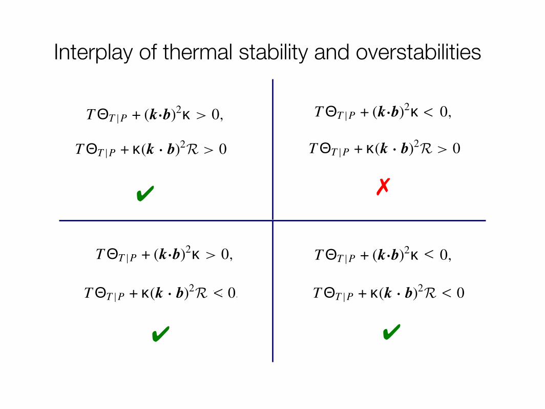
Interplay of thermal stability and overstabilities

No. 1, 2010 RADIATIVE AND DYNAMIC STABILITY OF A DILUTE PLASMA L99

where

N2 = ! 1!"

dP

dz

d ln P!!"

dz= g

d ln P (1!" )/" T

dz, (18)

C =!

" ! 1"

"#(k·b)2, (19)

K =#1 ! 2b2

z

$k2" + 2bxbzkxkz. (20)

This corresponds to Equation (13) of Q08, except, as noted,for the single appearance of the radiative !T |P term. (A lessgeneral version of this result was also presented in Balbus& Reynolds 2008.) The dispersion characterizes the linearresponse of a magnetized, thermally conducting radiative diluteplasma to incompressible disturbances.

2.3. Stability

2.3.1. Recovery of the Conductive Field Criterion

Expanding the dispersion relation (17) leads to

$ 3 + a1$2 + a2$ + a3 = 0, (21)

where

a1 =!

" ! 1"

"T !T |P + C, (22)

a2 = k2"

k2N2 + (k · vA)2, (23)

a3 = CKg

k2

d ln T

dz+ (k · vA)2a1. (24)

There are stable solutions to this dispersion relation if andonly if the following three criteria are met:

a1 > 0, a3 > 0, a1a2 > a3. (25)

This follows from a Routh–Hurwitz analysis, but can be seenmore easily by inspection: the first two are in fact elementary,while the third follows from self-consistently demanding purelyimaginary solutions to the cubic equation and then investigatingtheir behavior for infinitesimal real parts.

The physical interpretation of a1 > 0, or

T !T |P + (k·b)2# > 0, (26)

is the magnetized conduction variation of the classical thermalinstability criterion (Field 1965). Only the component of k alongthe field lines enters into the conduction term.

2.3.2. Recovery of the HBI and MTI

We next consider the physical interpretation of a3 > 0, or

CKg

k2

d ln T

dz+ (k · vA)2a1 > 0. (27)

In essence, this is the HBI/MTI criterion of Q08, but further(de)stabilized when the flow is (un)stable by the isobaric Fieldcriterion. This is a true instability if a3 is negative, with$ = !a3/a2 in the limit of large a2 > 0.

Equation (27) shows that thermal instability and the HBI/MTI are intimately linked. To be definite, consider the behaviorof the HBI. The discussion of Q08 explains how the distortion

of field lines leads to conductive cooling of a downwardly dis-placed fluid element (and vice versa for an upwardly displacedelement). It is this cooling that causes the convection associ-ated with the HBI. With radiative losses present, the coolingis enhanced on a downward displacement, and relative heat-ing is present on an upward displacement. In fact, we mayimagine now slowly turning on the magnetic field from dy-namically weak to strongly dominant. Then, the exponentiallygrowing instability transforms from the Q08 HBI to the classi-cal (nonoscillatory) thermal instability. The role of the magneticfield in mediating this transition is crucial.

2.3.3. Destabilization of Wave Modes by a Positive Thermal Gradient

We now return to the third criterion, a1a2 > a3. With a3 > 0,this criterion is a more stringent stability criterion than the first(a1 > 0), and hence replaces it.

When a2 is large and positive (e.g., either N2 or (k · vA)2

is dominant), the unstable roots depending on a1 will beapproximately

$ = ±ia1/22 + (a3 ! a1a2)/2a2. (28)

On the other hand, at large wavenumbers, we may have a1and a3 as the dominant terms. If a3 and a1 are both positive (orboth negative), then the wavelike solutions will be

$ = ±i(a3/a1)1/2 + (a3 ! a1a2)/2a21 . (29)

In either case above, the combination a3 ! a1a2 determinesthe stability of the mode.

After a cancellation of the magnetic tension terms, thecondition a1a2 ! a3 > 0 becomes

a1k2"

k2N2 ! CK

g

k2

d ln T

dz> 0. (30)

Consider the limit bz # 1, which is HBI stable (a3 > 0)for all but nearly axial wavenumbers, whose growth times thenbecome very long. (We cannot take bz = 0 exactly, since thatwould preclude a static radiative equilibrium state. For bz finite,Equation (10) shows that the equilibrium dT /dz scales as b!1

z .)Then, K = k2

", and our inequality reduces to

" ! 1"

T !T |P N2 + C!

N2 ! gd ln T

dz

"> 0. (31)

But

N2 ! gd ln T

dz= " ! 1

"

1P!

!dP

dz

"2

, (32)

and assuming that N2 > 0, the inequality may be yet furtherreduced:

T !T |P +C

!PN2

!dP

dz

"2

> 0. (33)

Finally, substituting for C and N2 and simplifying, ourcondition becomes

T !T |P + #(k · b)2R > 0, (34)

where R is the reduction factor

R =!

1 +%%%%

"

" ! 1d ln T

d ln P

%%%%

"!1

, (35)

No. 1, 2010 RADIATIVE AND DYNAMIC STABILITY OF A DILUTE PLASMA L99

where

N2 = ! 1!"

dP

dz

d ln P!!"

dz= g

d ln P (1!" )/" T

dz, (18)

C =!

" ! 1"

"#(k·b)2, (19)

K =#1 ! 2b2

z

$k2" + 2bxbzkxkz. (20)

This corresponds to Equation (13) of Q08, except, as noted,for the single appearance of the radiative !T |P term. (A lessgeneral version of this result was also presented in Balbus& Reynolds 2008.) The dispersion characterizes the linearresponse of a magnetized, thermally conducting radiative diluteplasma to incompressible disturbances.

2.3. Stability

2.3.1. Recovery of the Conductive Field Criterion

Expanding the dispersion relation (17) leads to

$ 3 + a1$2 + a2$ + a3 = 0, (21)

where

a1 =!

" ! 1"

"T !T |P + C, (22)

a2 = k2"

k2N2 + (k · vA)2, (23)

a3 = CKg

k2

d ln T

dz+ (k · vA)2a1. (24)

There are stable solutions to this dispersion relation if andonly if the following three criteria are met:

a1 > 0, a3 > 0, a1a2 > a3. (25)

This follows from a Routh–Hurwitz analysis, but can be seenmore easily by inspection: the first two are in fact elementary,while the third follows from self-consistently demanding purelyimaginary solutions to the cubic equation and then investigatingtheir behavior for infinitesimal real parts.

The physical interpretation of a1 > 0, or

T !T |P + (k·b)2# > 0, (26)

is the magnetized conduction variation of the classical thermalinstability criterion (Field 1965). Only the component of k alongthe field lines enters into the conduction term.

2.3.2. Recovery of the HBI and MTI

We next consider the physical interpretation of a3 > 0, or

CKg

k2

d ln T

dz+ (k · vA)2a1 > 0. (27)

In essence, this is the HBI/MTI criterion of Q08, but further(de)stabilized when the flow is (un)stable by the isobaric Fieldcriterion. This is a true instability if a3 is negative, with$ = !a3/a2 in the limit of large a2 > 0.

Equation (27) shows that thermal instability and the HBI/MTI are intimately linked. To be definite, consider the behaviorof the HBI. The discussion of Q08 explains how the distortion

of field lines leads to conductive cooling of a downwardly dis-placed fluid element (and vice versa for an upwardly displacedelement). It is this cooling that causes the convection associ-ated with the HBI. With radiative losses present, the coolingis enhanced on a downward displacement, and relative heat-ing is present on an upward displacement. In fact, we mayimagine now slowly turning on the magnetic field from dy-namically weak to strongly dominant. Then, the exponentiallygrowing instability transforms from the Q08 HBI to the classi-cal (nonoscillatory) thermal instability. The role of the magneticfield in mediating this transition is crucial.

2.3.3. Destabilization of Wave Modes by a Positive Thermal Gradient

We now return to the third criterion, a1a2 > a3. With a3 > 0,this criterion is a more stringent stability criterion than the first(a1 > 0), and hence replaces it.

When a2 is large and positive (e.g., either N2 or (k · vA)2

is dominant), the unstable roots depending on a1 will beapproximately

$ = ±ia1/22 + (a3 ! a1a2)/2a2. (28)

On the other hand, at large wavenumbers, we may have a1and a3 as the dominant terms. If a3 and a1 are both positive (orboth negative), then the wavelike solutions will be

$ = ±i(a3/a1)1/2 + (a3 ! a1a2)/2a21 . (29)

In either case above, the combination a3 ! a1a2 determinesthe stability of the mode.

After a cancellation of the magnetic tension terms, thecondition a1a2 ! a3 > 0 becomes

a1k2"

k2N2 ! CK

g

k2

d ln T

dz> 0. (30)

Consider the limit bz # 1, which is HBI stable (a3 > 0)for all but nearly axial wavenumbers, whose growth times thenbecome very long. (We cannot take bz = 0 exactly, since thatwould preclude a static radiative equilibrium state. For bz finite,Equation (10) shows that the equilibrium dT /dz scales as b!1

z .)Then, K = k2

", and our inequality reduces to

" ! 1"

T !T |P N2 + C!

N2 ! gd ln T

dz

"> 0. (31)

But

N2 ! gd ln T

dz= " ! 1

"

1P!

!dP

dz

"2

, (32)

and assuming that N2 > 0, the inequality may be yet furtherreduced:

T !T |P +C

!PN2

!dP

dz

"2

> 0. (33)

Finally, substituting for C and N2 and simplifying, ourcondition becomes

T !T |P + #(k · b)2R > 0, (34)

where R is the reduction factor

R =!

1 +%%%%

"

" ! 1d ln T

d ln P

%%%%

"!1

, (35)

No. 1, 2010 RADIATIVE AND DYNAMIC STABILITY OF A DILUTE PLASMA L99

where

N2 = ! 1!"

dP

dz

d ln P!!"

dz= g

d ln P (1!" )/" T

dz, (18)

C =!

" ! 1"

"#(k·b)2, (19)

K =#1 ! 2b2

z

$k2" + 2bxbzkxkz. (20)

This corresponds to Equation (13) of Q08, except, as noted,for the single appearance of the radiative !T |P term. (A lessgeneral version of this result was also presented in Balbus& Reynolds 2008.) The dispersion characterizes the linearresponse of a magnetized, thermally conducting radiative diluteplasma to incompressible disturbances.

2.3. Stability

2.3.1. Recovery of the Conductive Field Criterion

Expanding the dispersion relation (17) leads to

$ 3 + a1$2 + a2$ + a3 = 0, (21)

where

a1 =!

" ! 1"

"T !T |P + C, (22)

a2 = k2"

k2N2 + (k · vA)2, (23)

a3 = CKg

k2

d ln T

dz+ (k · vA)2a1. (24)

There are stable solutions to this dispersion relation if andonly if the following three criteria are met:

a1 > 0, a3 > 0, a1a2 > a3. (25)

This follows from a Routh–Hurwitz analysis, but can be seenmore easily by inspection: the first two are in fact elementary,while the third follows from self-consistently demanding purelyimaginary solutions to the cubic equation and then investigatingtheir behavior for infinitesimal real parts.

The physical interpretation of a1 > 0, or

T !T |P + (k·b)2# > 0, (26)

is the magnetized conduction variation of the classical thermalinstability criterion (Field 1965). Only the component of k alongthe field lines enters into the conduction term.

2.3.2. Recovery of the HBI and MTI

We next consider the physical interpretation of a3 > 0, or

CKg

k2

d ln T

dz+ (k · vA)2a1 > 0. (27)

In essence, this is the HBI/MTI criterion of Q08, but further(de)stabilized when the flow is (un)stable by the isobaric Fieldcriterion. This is a true instability if a3 is negative, with$ = !a3/a2 in the limit of large a2 > 0.

Equation (27) shows that thermal instability and the HBI/MTI are intimately linked. To be definite, consider the behaviorof the HBI. The discussion of Q08 explains how the distortion

of field lines leads to conductive cooling of a downwardly dis-placed fluid element (and vice versa for an upwardly displacedelement). It is this cooling that causes the convection associ-ated with the HBI. With radiative losses present, the coolingis enhanced on a downward displacement, and relative heat-ing is present on an upward displacement. In fact, we mayimagine now slowly turning on the magnetic field from dy-namically weak to strongly dominant. Then, the exponentiallygrowing instability transforms from the Q08 HBI to the classi-cal (nonoscillatory) thermal instability. The role of the magneticfield in mediating this transition is crucial.

2.3.3. Destabilization of Wave Modes by a Positive Thermal Gradient

We now return to the third criterion, a1a2 > a3. With a3 > 0,this criterion is a more stringent stability criterion than the first(a1 > 0), and hence replaces it.

When a2 is large and positive (e.g., either N2 or (k · vA)2

is dominant), the unstable roots depending on a1 will beapproximately

$ = ±ia1/22 + (a3 ! a1a2)/2a2. (28)

On the other hand, at large wavenumbers, we may have a1and a3 as the dominant terms. If a3 and a1 are both positive (orboth negative), then the wavelike solutions will be

$ = ±i(a3/a1)1/2 + (a3 ! a1a2)/2a21 . (29)

In either case above, the combination a3 ! a1a2 determinesthe stability of the mode.

After a cancellation of the magnetic tension terms, thecondition a1a2 ! a3 > 0 becomes

a1k2"

k2N2 ! CK

g

k2

d ln T

dz> 0. (30)

Consider the limit bz # 1, which is HBI stable (a3 > 0)for all but nearly axial wavenumbers, whose growth times thenbecome very long. (We cannot take bz = 0 exactly, since thatwould preclude a static radiative equilibrium state. For bz finite,Equation (10) shows that the equilibrium dT /dz scales as b!1

z .)Then, K = k2

", and our inequality reduces to

" ! 1"

T !T |P N2 + C!

N2 ! gd ln T

dz

"> 0. (31)

But

N2 ! gd ln T

dz= " ! 1

"

1P!

!dP

dz

"2

, (32)

and assuming that N2 > 0, the inequality may be yet furtherreduced:

T !T |P +C

!PN2

!dP

dz

"2

> 0. (33)

Finally, substituting for C and N2 and simplifying, ourcondition becomes

T !T |P + #(k · b)2R > 0, (34)

where R is the reduction factor

R =!

1 +%%%%

"

" ! 1d ln T

d ln P

%%%%

"!1

, (35)

No. 1, 2010 RADIATIVE AND DYNAMIC STABILITY OF A DILUTE PLASMA L99

where

N2 = ! 1!"

dP

dz

d ln P!!"

dz= g

d ln P (1!" )/" T

dz, (18)

C =!

" ! 1"

"#(k·b)2, (19)

K =#1 ! 2b2

z

$k2" + 2bxbzkxkz. (20)

This corresponds to Equation (13) of Q08, except, as noted,for the single appearance of the radiative !T |P term. (A lessgeneral version of this result was also presented in Balbus& Reynolds 2008.) The dispersion characterizes the linearresponse of a magnetized, thermally conducting radiative diluteplasma to incompressible disturbances.

2.3. Stability

2.3.1. Recovery of the Conductive Field Criterion

Expanding the dispersion relation (17) leads to

$ 3 + a1$2 + a2$ + a3 = 0, (21)

where

a1 =!

" ! 1"

"T !T |P + C, (22)

a2 = k2"

k2N2 + (k · vA)2, (23)

a3 = CKg

k2

d ln T

dz+ (k · vA)2a1. (24)

There are stable solutions to this dispersion relation if andonly if the following three criteria are met:

a1 > 0, a3 > 0, a1a2 > a3. (25)

This follows from a Routh–Hurwitz analysis, but can be seenmore easily by inspection: the first two are in fact elementary,while the third follows from self-consistently demanding purelyimaginary solutions to the cubic equation and then investigatingtheir behavior for infinitesimal real parts.

The physical interpretation of a1 > 0, or

T !T |P + (k·b)2# > 0, (26)

is the magnetized conduction variation of the classical thermalinstability criterion (Field 1965). Only the component of k alongthe field lines enters into the conduction term.

2.3.2. Recovery of the HBI and MTI

We next consider the physical interpretation of a3 > 0, or

CKg

k2

d ln T

dz+ (k · vA)2a1 > 0. (27)

In essence, this is the HBI/MTI criterion of Q08, but further(de)stabilized when the flow is (un)stable by the isobaric Fieldcriterion. This is a true instability if a3 is negative, with$ = !a3/a2 in the limit of large a2 > 0.

Equation (27) shows that thermal instability and the HBI/MTI are intimately linked. To be definite, consider the behaviorof the HBI. The discussion of Q08 explains how the distortion

of field lines leads to conductive cooling of a downwardly dis-placed fluid element (and vice versa for an upwardly displacedelement). It is this cooling that causes the convection associ-ated with the HBI. With radiative losses present, the coolingis enhanced on a downward displacement, and relative heat-ing is present on an upward displacement. In fact, we mayimagine now slowly turning on the magnetic field from dy-namically weak to strongly dominant. Then, the exponentiallygrowing instability transforms from the Q08 HBI to the classi-cal (nonoscillatory) thermal instability. The role of the magneticfield in mediating this transition is crucial.

2.3.3. Destabilization of Wave Modes by a Positive Thermal Gradient

We now return to the third criterion, a1a2 > a3. With a3 > 0,this criterion is a more stringent stability criterion than the first(a1 > 0), and hence replaces it.

When a2 is large and positive (e.g., either N2 or (k · vA)2

is dominant), the unstable roots depending on a1 will beapproximately

$ = ±ia1/22 + (a3 ! a1a2)/2a2. (28)

On the other hand, at large wavenumbers, we may have a1and a3 as the dominant terms. If a3 and a1 are both positive (orboth negative), then the wavelike solutions will be

$ = ±i(a3/a1)1/2 + (a3 ! a1a2)/2a21 . (29)

In either case above, the combination a3 ! a1a2 determinesthe stability of the mode.

After a cancellation of the magnetic tension terms, thecondition a1a2 ! a3 > 0 becomes

a1k2"

k2N2 ! CK

g

k2

d ln T

dz> 0. (30)

Consider the limit bz # 1, which is HBI stable (a3 > 0)for all but nearly axial wavenumbers, whose growth times thenbecome very long. (We cannot take bz = 0 exactly, since thatwould preclude a static radiative equilibrium state. For bz finite,Equation (10) shows that the equilibrium dT /dz scales as b!1

z .)Then, K = k2

", and our inequality reduces to

" ! 1"

T !T |P N2 + C!

N2 ! gd ln T

dz

"> 0. (31)

But

N2 ! gd ln T

dz= " ! 1

"

1P!

!dP

dz

"2

, (32)

and assuming that N2 > 0, the inequality may be yet furtherreduced:

T !T |P +C

!PN2

!dP

dz

"2

> 0. (33)

Finally, substituting for C and N2 and simplifying, ourcondition becomes

T !T |P + #(k · b)2R > 0, (34)

where R is the reduction factor

R =!

1 +%%%%

"

" ! 1d ln T

d ln P

%%%%

"!1

, (35)

No. 1, 2010 RADIATIVE AND DYNAMIC STABILITY OF A DILUTE PLASMA L99

where

N2 = ! 1!"

dP

dz

d ln P!!"

dz= g

d ln P (1!" )/" T

dz, (18)

C =!

" ! 1"

"#(k·b)2, (19)

K =#1 ! 2b2

z

$k2" + 2bxbzkxkz. (20)

This corresponds to Equation (13) of Q08, except, as noted,for the single appearance of the radiative !T |P term. (A lessgeneral version of this result was also presented in Balbus& Reynolds 2008.) The dispersion characterizes the linearresponse of a magnetized, thermally conducting radiative diluteplasma to incompressible disturbances.

2.3. Stability

2.3.1. Recovery of the Conductive Field Criterion

Expanding the dispersion relation (17) leads to

$ 3 + a1$2 + a2$ + a3 = 0, (21)

where

a1 =!

" ! 1"

"T !T |P + C, (22)

a2 = k2"

k2N2 + (k · vA)2, (23)

a3 = CKg

k2

d ln T

dz+ (k · vA)2a1. (24)

There are stable solutions to this dispersion relation if andonly if the following three criteria are met:

a1 > 0, a3 > 0, a1a2 > a3. (25)

This follows from a Routh–Hurwitz analysis, but can be seenmore easily by inspection: the first two are in fact elementary,while the third follows from self-consistently demanding purelyimaginary solutions to the cubic equation and then investigatingtheir behavior for infinitesimal real parts.

The physical interpretation of a1 > 0, or

T !T |P + (k·b)2# > 0, (26)

is the magnetized conduction variation of the classical thermalinstability criterion (Field 1965). Only the component of k alongthe field lines enters into the conduction term.

2.3.2. Recovery of the HBI and MTI

We next consider the physical interpretation of a3 > 0, or

CKg

k2

d ln T

dz+ (k · vA)2a1 > 0. (27)

In essence, this is the HBI/MTI criterion of Q08, but further(de)stabilized when the flow is (un)stable by the isobaric Fieldcriterion. This is a true instability if a3 is negative, with$ = !a3/a2 in the limit of large a2 > 0.

Equation (27) shows that thermal instability and the HBI/MTI are intimately linked. To be definite, consider the behaviorof the HBI. The discussion of Q08 explains how the distortion

of field lines leads to conductive cooling of a downwardly dis-placed fluid element (and vice versa for an upwardly displacedelement). It is this cooling that causes the convection associ-ated with the HBI. With radiative losses present, the coolingis enhanced on a downward displacement, and relative heat-ing is present on an upward displacement. In fact, we mayimagine now slowly turning on the magnetic field from dy-namically weak to strongly dominant. Then, the exponentiallygrowing instability transforms from the Q08 HBI to the classi-cal (nonoscillatory) thermal instability. The role of the magneticfield in mediating this transition is crucial.

2.3.3. Destabilization of Wave Modes by a Positive Thermal Gradient

We now return to the third criterion, a1a2 > a3. With a3 > 0,this criterion is a more stringent stability criterion than the first(a1 > 0), and hence replaces it.

When a2 is large and positive (e.g., either N2 or (k · vA)2

is dominant), the unstable roots depending on a1 will beapproximately

$ = ±ia1/22 + (a3 ! a1a2)/2a2. (28)

On the other hand, at large wavenumbers, we may have a1and a3 as the dominant terms. If a3 and a1 are both positive (orboth negative), then the wavelike solutions will be

$ = ±i(a3/a1)1/2 + (a3 ! a1a2)/2a21 . (29)

In either case above, the combination a3 ! a1a2 determinesthe stability of the mode.

After a cancellation of the magnetic tension terms, thecondition a1a2 ! a3 > 0 becomes

a1k2"

k2N2 ! CK

g

k2

d ln T

dz> 0. (30)

Consider the limit bz # 1, which is HBI stable (a3 > 0)for all but nearly axial wavenumbers, whose growth times thenbecome very long. (We cannot take bz = 0 exactly, since thatwould preclude a static radiative equilibrium state. For bz finite,Equation (10) shows that the equilibrium dT /dz scales as b!1

z .)Then, K = k2

", and our inequality reduces to

" ! 1"

T !T |P N2 + C!

N2 ! gd ln T

dz

"> 0. (31)

But

N2 ! gd ln T

dz= " ! 1

"

1P!

!dP

dz

"2

, (32)

and assuming that N2 > 0, the inequality may be yet furtherreduced:

T !T |P +C

!PN2

!dP

dz

"2

> 0. (33)

Finally, substituting for C and N2 and simplifying, ourcondition becomes

T !T |P + #(k · b)2R > 0, (34)

where R is the reduction factor

R =!

1 +%%%%

"

" ! 1d ln T

d ln P

%%%%

"!1

, (35)

<

No. 1, 2010 RADIATIVE AND DYNAMIC STABILITY OF A DILUTE PLASMA L99

where

N2 = ! 1!"

dP

dz

d ln P!!"

dz= g

d ln P (1!" )/" T

dz, (18)

C =!

" ! 1"

"#(k·b)2, (19)

K =#1 ! 2b2

z

$k2" + 2bxbzkxkz. (20)

This corresponds to Equation (13) of Q08, except, as noted,for the single appearance of the radiative !T |P term. (A lessgeneral version of this result was also presented in Balbus& Reynolds 2008.) The dispersion characterizes the linearresponse of a magnetized, thermally conducting radiative diluteplasma to incompressible disturbances.

2.3. Stability

2.3.1. Recovery of the Conductive Field Criterion

Expanding the dispersion relation (17) leads to

$ 3 + a1$2 + a2$ + a3 = 0, (21)

where

a1 =!

" ! 1"

"T !T |P + C, (22)

a2 = k2"

k2N2 + (k · vA)2, (23)

a3 = CKg

k2

d ln T

dz+ (k · vA)2a1. (24)

There are stable solutions to this dispersion relation if andonly if the following three criteria are met:

a1 > 0, a3 > 0, a1a2 > a3. (25)

This follows from a Routh–Hurwitz analysis, but can be seenmore easily by inspection: the first two are in fact elementary,while the third follows from self-consistently demanding purelyimaginary solutions to the cubic equation and then investigatingtheir behavior for infinitesimal real parts.

The physical interpretation of a1 > 0, or

T !T |P + (k·b)2# > 0, (26)

is the magnetized conduction variation of the classical thermalinstability criterion (Field 1965). Only the component of k alongthe field lines enters into the conduction term.

2.3.2. Recovery of the HBI and MTI

We next consider the physical interpretation of a3 > 0, or

CKg

k2

d ln T

dz+ (k · vA)2a1 > 0. (27)

In essence, this is the HBI/MTI criterion of Q08, but further(de)stabilized when the flow is (un)stable by the isobaric Fieldcriterion. This is a true instability if a3 is negative, with$ = !a3/a2 in the limit of large a2 > 0.

Equation (27) shows that thermal instability and the HBI/MTI are intimately linked. To be definite, consider the behaviorof the HBI. The discussion of Q08 explains how the distortion

of field lines leads to conductive cooling of a downwardly dis-placed fluid element (and vice versa for an upwardly displacedelement). It is this cooling that causes the convection associ-ated with the HBI. With radiative losses present, the coolingis enhanced on a downward displacement, and relative heat-ing is present on an upward displacement. In fact, we mayimagine now slowly turning on the magnetic field from dy-namically weak to strongly dominant. Then, the exponentiallygrowing instability transforms from the Q08 HBI to the classi-cal (nonoscillatory) thermal instability. The role of the magneticfield in mediating this transition is crucial.

2.3.3. Destabilization of Wave Modes by a Positive Thermal Gradient

We now return to the third criterion, a1a2 > a3. With a3 > 0,this criterion is a more stringent stability criterion than the first(a1 > 0), and hence replaces it.

When a2 is large and positive (e.g., either N2 or (k · vA)2

is dominant), the unstable roots depending on a1 will beapproximately

$ = ±ia1/22 + (a3 ! a1a2)/2a2. (28)

On the other hand, at large wavenumbers, we may have a1and a3 as the dominant terms. If a3 and a1 are both positive (orboth negative), then the wavelike solutions will be

$ = ±i(a3/a1)1/2 + (a3 ! a1a2)/2a21 . (29)

In either case above, the combination a3 ! a1a2 determinesthe stability of the mode.

After a cancellation of the magnetic tension terms, thecondition a1a2 ! a3 > 0 becomes

a1k2"

k2N2 ! CK

g

k2

d ln T

dz> 0. (30)

Consider the limit bz # 1, which is HBI stable (a3 > 0)for all but nearly axial wavenumbers, whose growth times thenbecome very long. (We cannot take bz = 0 exactly, since thatwould preclude a static radiative equilibrium state. For bz finite,Equation (10) shows that the equilibrium dT /dz scales as b!1

z .)Then, K = k2

", and our inequality reduces to

" ! 1"

T !T |P N2 + C!

N2 ! gd ln T

dz

"> 0. (31)

But

N2 ! gd ln T

dz= " ! 1

"

1P!

!dP

dz

"2

, (32)

and assuming that N2 > 0, the inequality may be yet furtherreduced:

T !T |P +C

!PN2

!dP

dz

"2

> 0. (33)

Finally, substituting for C and N2 and simplifying, ourcondition becomes

T !T |P + #(k · b)2R > 0, (34)

where R is the reduction factor

R =!

1 +%%%%

"

" ! 1d ln T

d ln P

%%%%

"!1

, (35)

<

No. 1, 2010 RADIATIVE AND DYNAMIC STABILITY OF A DILUTE PLASMA L99

where

N2 = ! 1!"

dP

dz

d ln P!!"

dz= g

d ln P (1!" )/" T

dz, (18)

C =!

" ! 1"

"#(k·b)2, (19)

K =#1 ! 2b2

z

$k2" + 2bxbzkxkz. (20)

This corresponds to Equation (13) of Q08, except, as noted,for the single appearance of the radiative !T |P term. (A lessgeneral version of this result was also presented in Balbus& Reynolds 2008.) The dispersion characterizes the linearresponse of a magnetized, thermally conducting radiative diluteplasma to incompressible disturbances.

2.3. Stability

2.3.1. Recovery of the Conductive Field Criterion

Expanding the dispersion relation (17) leads to

$ 3 + a1$2 + a2$ + a3 = 0, (21)

where

a1 =!

" ! 1"

"T !T |P + C, (22)

a2 = k2"

k2N2 + (k · vA)2, (23)

a3 = CKg

k2

d ln T

dz+ (k · vA)2a1. (24)

There are stable solutions to this dispersion relation if andonly if the following three criteria are met:

a1 > 0, a3 > 0, a1a2 > a3. (25)

This follows from a Routh–Hurwitz analysis, but can be seenmore easily by inspection: the first two are in fact elementary,while the third follows from self-consistently demanding purelyimaginary solutions to the cubic equation and then investigatingtheir behavior for infinitesimal real parts.

The physical interpretation of a1 > 0, or

T !T |P + (k·b)2# > 0, (26)

is the magnetized conduction variation of the classical thermalinstability criterion (Field 1965). Only the component of k alongthe field lines enters into the conduction term.

2.3.2. Recovery of the HBI and MTI

We next consider the physical interpretation of a3 > 0, or

CKg

k2

d ln T

dz+ (k · vA)2a1 > 0. (27)

In essence, this is the HBI/MTI criterion of Q08, but further(de)stabilized when the flow is (un)stable by the isobaric Fieldcriterion. This is a true instability if a3 is negative, with$ = !a3/a2 in the limit of large a2 > 0.

Equation (27) shows that thermal instability and the HBI/MTI are intimately linked. To be definite, consider the behaviorof the HBI. The discussion of Q08 explains how the distortion

of field lines leads to conductive cooling of a downwardly dis-placed fluid element (and vice versa for an upwardly displacedelement). It is this cooling that causes the convection associ-ated with the HBI. With radiative losses present, the coolingis enhanced on a downward displacement, and relative heat-ing is present on an upward displacement. In fact, we mayimagine now slowly turning on the magnetic field from dy-namically weak to strongly dominant. Then, the exponentiallygrowing instability transforms from the Q08 HBI to the classi-cal (nonoscillatory) thermal instability. The role of the magneticfield in mediating this transition is crucial.

2.3.3. Destabilization of Wave Modes by a Positive Thermal Gradient

We now return to the third criterion, a1a2 > a3. With a3 > 0,this criterion is a more stringent stability criterion than the first(a1 > 0), and hence replaces it.

When a2 is large and positive (e.g., either N2 or (k · vA)2

is dominant), the unstable roots depending on a1 will beapproximately

$ = ±ia1/22 + (a3 ! a1a2)/2a2. (28)

On the other hand, at large wavenumbers, we may have a1and a3 as the dominant terms. If a3 and a1 are both positive (orboth negative), then the wavelike solutions will be

$ = ±i(a3/a1)1/2 + (a3 ! a1a2)/2a21 . (29)

In either case above, the combination a3 ! a1a2 determinesthe stability of the mode.

After a cancellation of the magnetic tension terms, thecondition a1a2 ! a3 > 0 becomes

a1k2"

k2N2 ! CK

g

k2

d ln T

dz> 0. (30)

Consider the limit bz # 1, which is HBI stable (a3 > 0)for all but nearly axial wavenumbers, whose growth times thenbecome very long. (We cannot take bz = 0 exactly, since thatwould preclude a static radiative equilibrium state. For bz finite,Equation (10) shows that the equilibrium dT /dz scales as b!1

z .)Then, K = k2

", and our inequality reduces to

" ! 1"

T !T |P N2 + C!

N2 ! gd ln T

dz

"> 0. (31)

But

N2 ! gd ln T

dz= " ! 1

"

1P!

!dP

dz

"2

, (32)

and assuming that N2 > 0, the inequality may be yet furtherreduced:

T !T |P +C

!PN2

!dP

dz

"2

> 0. (33)

Finally, substituting for C and N2 and simplifying, ourcondition becomes

T !T |P + #(k · b)2R > 0, (34)

where R is the reduction factor

R =!

1 +%%%%

"

" ! 1d ln T

d ln P

%%%%

"!1

, (35)

<

No. 1, 2010 RADIATIVE AND DYNAMIC STABILITY OF A DILUTE PLASMA L99

where

N2 = ! 1!"

dP

dz

d ln P!!"

dz= g

d ln P (1!" )/" T

dz, (18)

C =!

" ! 1"

"#(k·b)2, (19)

K =#1 ! 2b2

z

$k2" + 2bxbzkxkz. (20)

This corresponds to Equation (13) of Q08, except, as noted,for the single appearance of the radiative !T |P term. (A lessgeneral version of this result was also presented in Balbus& Reynolds 2008.) The dispersion characterizes the linearresponse of a magnetized, thermally conducting radiative diluteplasma to incompressible disturbances.

2.3. Stability

2.3.1. Recovery of the Conductive Field Criterion

Expanding the dispersion relation (17) leads to

$ 3 + a1$2 + a2$ + a3 = 0, (21)

where

a1 =!

" ! 1"

"T !T |P + C, (22)

a2 = k2"

k2N2 + (k · vA)2, (23)

a3 = CKg

k2

d ln T

dz+ (k · vA)2a1. (24)

There are stable solutions to this dispersion relation if andonly if the following three criteria are met:

a1 > 0, a3 > 0, a1a2 > a3. (25)

This follows from a Routh–Hurwitz analysis, but can be seenmore easily by inspection: the first two are in fact elementary,while the third follows from self-consistently demanding purelyimaginary solutions to the cubic equation and then investigatingtheir behavior for infinitesimal real parts.

The physical interpretation of a1 > 0, or

T !T |P + (k·b)2# > 0, (26)

is the magnetized conduction variation of the classical thermalinstability criterion (Field 1965). Only the component of k alongthe field lines enters into the conduction term.

2.3.2. Recovery of the HBI and MTI

We next consider the physical interpretation of a3 > 0, or

CKg

k2

d ln T

dz+ (k · vA)2a1 > 0. (27)

In essence, this is the HBI/MTI criterion of Q08, but further(de)stabilized when the flow is (un)stable by the isobaric Fieldcriterion. This is a true instability if a3 is negative, with$ = !a3/a2 in the limit of large a2 > 0.

Equation (27) shows that thermal instability and the HBI/MTI are intimately linked. To be definite, consider the behaviorof the HBI. The discussion of Q08 explains how the distortion

of field lines leads to conductive cooling of a downwardly dis-placed fluid element (and vice versa for an upwardly displacedelement). It is this cooling that causes the convection associ-ated with the HBI. With radiative losses present, the coolingis enhanced on a downward displacement, and relative heat-ing is present on an upward displacement. In fact, we mayimagine now slowly turning on the magnetic field from dy-namically weak to strongly dominant. Then, the exponentiallygrowing instability transforms from the Q08 HBI to the classi-cal (nonoscillatory) thermal instability. The role of the magneticfield in mediating this transition is crucial.

2.3.3. Destabilization of Wave Modes by a Positive Thermal Gradient

We now return to the third criterion, a1a2 > a3. With a3 > 0,this criterion is a more stringent stability criterion than the first(a1 > 0), and hence replaces it.

When a2 is large and positive (e.g., either N2 or (k · vA)2

is dominant), the unstable roots depending on a1 will beapproximately

$ = ±ia1/22 + (a3 ! a1a2)/2a2. (28)

On the other hand, at large wavenumbers, we may have a1and a3 as the dominant terms. If a3 and a1 are both positive (orboth negative), then the wavelike solutions will be

$ = ±i(a3/a1)1/2 + (a3 ! a1a2)/2a21 . (29)

In either case above, the combination a3 ! a1a2 determinesthe stability of the mode.

After a cancellation of the magnetic tension terms, thecondition a1a2 ! a3 > 0 becomes

a1k2"

k2N2 ! CK

g

k2

d ln T

dz> 0. (30)

Consider the limit bz # 1, which is HBI stable (a3 > 0)for all but nearly axial wavenumbers, whose growth times thenbecome very long. (We cannot take bz = 0 exactly, since thatwould preclude a static radiative equilibrium state. For bz finite,Equation (10) shows that the equilibrium dT /dz scales as b!1

z .)Then, K = k2

", and our inequality reduces to

" ! 1"

T !T |P N2 + C!

N2 ! gd ln T

dz

"> 0. (31)

But

N2 ! gd ln T

dz= " ! 1

"

1P!

!dP

dz

"2

, (32)

and assuming that N2 > 0, the inequality may be yet furtherreduced:

T !T |P +C

!PN2

!dP

dz

"2

> 0. (33)

Finally, substituting for C and N2 and simplifying, ourcondition becomes

T !T |P + #(k · b)2R > 0, (34)

where R is the reduction factor

R =!

1 +%%%%

"

" ! 1d ln T

d ln P

%%%%

"!1

, (35)

<

✔

✔ ✔

✗

Interplay of thermal stability and overstabilities

No. 1, 2010 RADIATIVE AND DYNAMIC STABILITY OF A DILUTE PLASMA L99

where

N2 = ! 1!"

dP

dz

d ln P!!"

dz= g

d ln P (1!" )/" T

dz, (18)

C =!

" ! 1"

"#(k·b)2, (19)

K =#1 ! 2b2

z

$k2" + 2bxbzkxkz. (20)

This corresponds to Equation (13) of Q08, except, as noted,for the single appearance of the radiative !T |P term. (A lessgeneral version of this result was also presented in Balbus& Reynolds 2008.) The dispersion characterizes the linearresponse of a magnetized, thermally conducting radiative diluteplasma to incompressible disturbances.

2.3. Stability

2.3.1. Recovery of the Conductive Field Criterion

Expanding the dispersion relation (17) leads to

$ 3 + a1$2 + a2$ + a3 = 0, (21)

where

a1 =!

" ! 1"

"T !T |P + C, (22)

a2 = k2"

k2N2 + (k · vA)2, (23)

a3 = CKg

k2

d ln T

dz+ (k · vA)2a1. (24)

There are stable solutions to this dispersion relation if andonly if the following three criteria are met:

a1 > 0, a3 > 0, a1a2 > a3. (25)

This follows from a Routh–Hurwitz analysis, but can be seenmore easily by inspection: the first two are in fact elementary,while the third follows from self-consistently demanding purelyimaginary solutions to the cubic equation and then investigatingtheir behavior for infinitesimal real parts.

The physical interpretation of a1 > 0, or

T !T |P + (k·b)2# > 0, (26)

is the magnetized conduction variation of the classical thermalinstability criterion (Field 1965). Only the component of k alongthe field lines enters into the conduction term.

2.3.2. Recovery of the HBI and MTI

We next consider the physical interpretation of a3 > 0, or

CKg

k2

d ln T

dz+ (k · vA)2a1 > 0. (27)

In essence, this is the HBI/MTI criterion of Q08, but further(de)stabilized when the flow is (un)stable by the isobaric Fieldcriterion. This is a true instability if a3 is negative, with$ = !a3/a2 in the limit of large a2 > 0.

Equation (27) shows that thermal instability and the HBI/MTI are intimately linked. To be definite, consider the behaviorof the HBI. The discussion of Q08 explains how the distortion

of field lines leads to conductive cooling of a downwardly dis-placed fluid element (and vice versa for an upwardly displacedelement). It is this cooling that causes the convection associ-ated with the HBI. With radiative losses present, the coolingis enhanced on a downward displacement, and relative heat-ing is present on an upward displacement. In fact, we mayimagine now slowly turning on the magnetic field from dy-namically weak to strongly dominant. Then, the exponentiallygrowing instability transforms from the Q08 HBI to the classi-cal (nonoscillatory) thermal instability. The role of the magneticfield in mediating this transition is crucial.

2.3.3. Destabilization of Wave Modes by a Positive Thermal Gradient

We now return to the third criterion, a1a2 > a3. With a3 > 0,this criterion is a more stringent stability criterion than the first(a1 > 0), and hence replaces it.

When a2 is large and positive (e.g., either N2 or (k · vA)2

is dominant), the unstable roots depending on a1 will beapproximately

$ = ±ia1/22 + (a3 ! a1a2)/2a2. (28)

On the other hand, at large wavenumbers, we may have a1and a3 as the dominant terms. If a3 and a1 are both positive (orboth negative), then the wavelike solutions will be

$ = ±i(a3/a1)1/2 + (a3 ! a1a2)/2a21 . (29)

In either case above, the combination a3 ! a1a2 determinesthe stability of the mode.

After a cancellation of the magnetic tension terms, thecondition a1a2 ! a3 > 0 becomes

a1k2"

k2N2 ! CK

g

k2

d ln T

dz> 0. (30)

Consider the limit bz # 1, which is HBI stable (a3 > 0)for all but nearly axial wavenumbers, whose growth times thenbecome very long. (We cannot take bz = 0 exactly, since thatwould preclude a static radiative equilibrium state. For bz finite,Equation (10) shows that the equilibrium dT /dz scales as b!1

z .)Then, K = k2

", and our inequality reduces to

" ! 1"

T !T |P N2 + C!

N2 ! gd ln T

dz

"> 0. (31)

But

N2 ! gd ln T

dz= " ! 1

"

1P!

!dP

dz

"2

, (32)

and assuming that N2 > 0, the inequality may be yet furtherreduced:

T !T |P +C

!PN2

!dP

dz

"2

> 0. (33)

Finally, substituting for C and N2 and simplifying, ourcondition becomes

T !T |P + #(k · b)2R > 0, (34)

where R is the reduction factor

R =!

1 +%%%%

"

" ! 1d ln T

d ln P

%%%%

"!1

, (35)

No. 1, 2010 RADIATIVE AND DYNAMIC STABILITY OF A DILUTE PLASMA L99

where

N2 = ! 1!"

dP

dz

d ln P!!"

dz= g

d ln P (1!" )/" T

dz, (18)

C =!

" ! 1"

"#(k·b)2, (19)

K =#1 ! 2b2

z

$k2" + 2bxbzkxkz. (20)

This corresponds to Equation (13) of Q08, except, as noted,for the single appearance of the radiative !T |P term. (A lessgeneral version of this result was also presented in Balbus& Reynolds 2008.) The dispersion characterizes the linearresponse of a magnetized, thermally conducting radiative diluteplasma to incompressible disturbances.

2.3. Stability

2.3.1. Recovery of the Conductive Field Criterion

Expanding the dispersion relation (17) leads to

$ 3 + a1$2 + a2$ + a3 = 0, (21)

where

a1 =!

" ! 1"

"T !T |P + C, (22)

a2 = k2"

k2N2 + (k · vA)2, (23)

a3 = CKg

k2

d ln T

dz+ (k · vA)2a1. (24)

There are stable solutions to this dispersion relation if andonly if the following three criteria are met:

a1 > 0, a3 > 0, a1a2 > a3. (25)

This follows from a Routh–Hurwitz analysis, but can be seenmore easily by inspection: the first two are in fact elementary,while the third follows from self-consistently demanding purelyimaginary solutions to the cubic equation and then investigatingtheir behavior for infinitesimal real parts.

The physical interpretation of a1 > 0, or

T !T |P + (k·b)2# > 0, (26)

is the magnetized conduction variation of the classical thermalinstability criterion (Field 1965). Only the component of k alongthe field lines enters into the conduction term.

2.3.2. Recovery of the HBI and MTI

We next consider the physical interpretation of a3 > 0, or

CKg

k2

d ln T

dz+ (k · vA)2a1 > 0. (27)

In essence, this is the HBI/MTI criterion of Q08, but further(de)stabilized when the flow is (un)stable by the isobaric Fieldcriterion. This is a true instability if a3 is negative, with$ = !a3/a2 in the limit of large a2 > 0.

Equation (27) shows that thermal instability and the HBI/MTI are intimately linked. To be definite, consider the behaviorof the HBI. The discussion of Q08 explains how the distortion

of field lines leads to conductive cooling of a downwardly dis-placed fluid element (and vice versa for an upwardly displacedelement). It is this cooling that causes the convection associ-ated with the HBI. With radiative losses present, the coolingis enhanced on a downward displacement, and relative heat-ing is present on an upward displacement. In fact, we mayimagine now slowly turning on the magnetic field from dy-namically weak to strongly dominant. Then, the exponentiallygrowing instability transforms from the Q08 HBI to the classi-cal (nonoscillatory) thermal instability. The role of the magneticfield in mediating this transition is crucial.

2.3.3. Destabilization of Wave Modes by a Positive Thermal Gradient

We now return to the third criterion, a1a2 > a3. With a3 > 0,this criterion is a more stringent stability criterion than the first(a1 > 0), and hence replaces it.

When a2 is large and positive (e.g., either N2 or (k · vA)2

is dominant), the unstable roots depending on a1 will beapproximately

$ = ±ia1/22 + (a3 ! a1a2)/2a2. (28)

On the other hand, at large wavenumbers, we may have a1and a3 as the dominant terms. If a3 and a1 are both positive (orboth negative), then the wavelike solutions will be

$ = ±i(a3/a1)1/2 + (a3 ! a1a2)/2a21 . (29)

In either case above, the combination a3 ! a1a2 determinesthe stability of the mode.

After a cancellation of the magnetic tension terms, thecondition a1a2 ! a3 > 0 becomes

a1k2"

k2N2 ! CK

g

k2

d ln T

dz> 0. (30)

Consider the limit bz # 1, which is HBI stable (a3 > 0)for all but nearly axial wavenumbers, whose growth times thenbecome very long. (We cannot take bz = 0 exactly, since thatwould preclude a static radiative equilibrium state. For bz finite,Equation (10) shows that the equilibrium dT /dz scales as b!1

z .)Then, K = k2

", and our inequality reduces to

" ! 1"

T !T |P N2 + C!

N2 ! gd ln T

dz

"> 0. (31)

But

N2 ! gd ln T

dz= " ! 1

"

1P!

!dP

dz

"2

, (32)

and assuming that N2 > 0, the inequality may be yet furtherreduced:

T !T |P +C

!PN2

!dP

dz

"2

> 0. (33)

Finally, substituting for C and N2 and simplifying, ourcondition becomes

T !T |P + #(k · b)2R > 0, (34)

where R is the reduction factor

R =!

1 +%%%%

"

" ! 1d ln T

d ln P

%%%%

"!1

, (35)

No. 1, 2010 RADIATIVE AND DYNAMIC STABILITY OF A DILUTE PLASMA L99

where

N2 = ! 1!"

dP

dz

d ln P!!"

dz= g

d ln P (1!" )/" T

dz, (18)

C =!

" ! 1"

"#(k·b)2, (19)

K =#1 ! 2b2

z

$k2" + 2bxbzkxkz. (20)

This corresponds to Equation (13) of Q08, except, as noted,for the single appearance of the radiative !T |P term. (A lessgeneral version of this result was also presented in Balbus& Reynolds 2008.) The dispersion characterizes the linearresponse of a magnetized, thermally conducting radiative diluteplasma to incompressible disturbances.

2.3. Stability

2.3.1. Recovery of the Conductive Field Criterion

Expanding the dispersion relation (17) leads to

$ 3 + a1$2 + a2$ + a3 = 0, (21)

where

a1 =!

" ! 1"

"T !T |P + C, (22)

a2 = k2"

k2N2 + (k · vA)2, (23)

a3 = CKg

k2

d ln T

dz+ (k · vA)2a1. (24)

There are stable solutions to this dispersion relation if andonly if the following three criteria are met:

a1 > 0, a3 > 0, a1a2 > a3. (25)

This follows from a Routh–Hurwitz analysis, but can be seenmore easily by inspection: the first two are in fact elementary,while the third follows from self-consistently demanding purelyimaginary solutions to the cubic equation and then investigatingtheir behavior for infinitesimal real parts.

The physical interpretation of a1 > 0, or

T !T |P + (k·b)2# > 0, (26)

is the magnetized conduction variation of the classical thermalinstability criterion (Field 1965). Only the component of k alongthe field lines enters into the conduction term.

2.3.2. Recovery of the HBI and MTI

We next consider the physical interpretation of a3 > 0, or

CKg

k2

d ln T

dz+ (k · vA)2a1 > 0. (27)

In essence, this is the HBI/MTI criterion of Q08, but further(de)stabilized when the flow is (un)stable by the isobaric Fieldcriterion. This is a true instability if a3 is negative, with$ = !a3/a2 in the limit of large a2 > 0.

Equation (27) shows that thermal instability and the HBI/MTI are intimately linked. To be definite, consider the behaviorof the HBI. The discussion of Q08 explains how the distortion

of field lines leads to conductive cooling of a downwardly dis-placed fluid element (and vice versa for an upwardly displacedelement). It is this cooling that causes the convection associ-ated with the HBI. With radiative losses present, the coolingis enhanced on a downward displacement, and relative heat-ing is present on an upward displacement. In fact, we mayimagine now slowly turning on the magnetic field from dy-namically weak to strongly dominant. Then, the exponentiallygrowing instability transforms from the Q08 HBI to the classi-cal (nonoscillatory) thermal instability. The role of the magneticfield in mediating this transition is crucial.

2.3.3. Destabilization of Wave Modes by a Positive Thermal Gradient

We now return to the third criterion, a1a2 > a3. With a3 > 0,this criterion is a more stringent stability criterion than the first(a1 > 0), and hence replaces it.

When a2 is large and positive (e.g., either N2 or (k · vA)2

is dominant), the unstable roots depending on a1 will beapproximately

$ = ±ia1/22 + (a3 ! a1a2)/2a2. (28)

On the other hand, at large wavenumbers, we may have a1and a3 as the dominant terms. If a3 and a1 are both positive (orboth negative), then the wavelike solutions will be

$ = ±i(a3/a1)1/2 + (a3 ! a1a2)/2a21 . (29)

In either case above, the combination a3 ! a1a2 determinesthe stability of the mode.

After a cancellation of the magnetic tension terms, thecondition a1a2 ! a3 > 0 becomes

a1k2"

k2N2 ! CK

g

k2

d ln T

dz> 0. (30)

Consider the limit bz # 1, which is HBI stable (a3 > 0)for all but nearly axial wavenumbers, whose growth times thenbecome very long. (We cannot take bz = 0 exactly, since thatwould preclude a static radiative equilibrium state. For bz finite,Equation (10) shows that the equilibrium dT /dz scales as b!1

z .)Then, K = k2

", and our inequality reduces to

" ! 1"

T !T |P N2 + C!

N2 ! gd ln T

dz

"> 0. (31)

But

N2 ! gd ln T

dz= " ! 1

"

1P!

!dP

dz

"2

, (32)

and assuming that N2 > 0, the inequality may be yet furtherreduced:

T !T |P +C

!PN2

!dP

dz

"2

> 0. (33)

Finally, substituting for C and N2 and simplifying, ourcondition becomes

T !T |P + #(k · b)2R > 0, (34)

where R is the reduction factor

R =!

1 +%%%%

"

" ! 1d ln T

d ln P

%%%%

"!1

, (35)

No. 1, 2010 RADIATIVE AND DYNAMIC STABILITY OF A DILUTE PLASMA L99

where

N2 = ! 1!"

dP

dz

d ln P!!"

dz= g

d ln P (1!" )/" T

dz, (18)

C =!

" ! 1"

"#(k·b)2, (19)

K =#1 ! 2b2

z

$k2" + 2bxbzkxkz. (20)

This corresponds to Equation (13) of Q08, except, as noted,for the single appearance of the radiative !T |P term. (A lessgeneral version of this result was also presented in Balbus& Reynolds 2008.) The dispersion characterizes the linearresponse of a magnetized, thermally conducting radiative diluteplasma to incompressible disturbances.

2.3. Stability

2.3.1. Recovery of the Conductive Field Criterion

Expanding the dispersion relation (17) leads to

$ 3 + a1$2 + a2$ + a3 = 0, (21)

where

a1 =!

" ! 1"

"T !T |P + C, (22)

a2 = k2"

k2N2 + (k · vA)2, (23)

a3 = CKg

k2

d ln T

dz+ (k · vA)2a1. (24)

There are stable solutions to this dispersion relation if andonly if the following three criteria are met:

a1 > 0, a3 > 0, a1a2 > a3. (25)

This follows from a Routh–Hurwitz analysis, but can be seenmore easily by inspection: the first two are in fact elementary,while the third follows from self-consistently demanding purelyimaginary solutions to the cubic equation and then investigatingtheir behavior for infinitesimal real parts.

The physical interpretation of a1 > 0, or

T !T |P + (k·b)2# > 0, (26)

is the magnetized conduction variation of the classical thermalinstability criterion (Field 1965). Only the component of k alongthe field lines enters into the conduction term.

2.3.2. Recovery of the HBI and MTI

We next consider the physical interpretation of a3 > 0, or

CKg

k2

d ln T

dz+ (k · vA)2a1 > 0. (27)

In essence, this is the HBI/MTI criterion of Q08, but further(de)stabilized when the flow is (un)stable by the isobaric Fieldcriterion. This is a true instability if a3 is negative, with$ = !a3/a2 in the limit of large a2 > 0.

Equation (27) shows that thermal instability and the HBI/MTI are intimately linked. To be definite, consider the behaviorof the HBI. The discussion of Q08 explains how the distortion

of field lines leads to conductive cooling of a downwardly dis-placed fluid element (and vice versa for an upwardly displacedelement). It is this cooling that causes the convection associ-ated with the HBI. With radiative losses present, the coolingis enhanced on a downward displacement, and relative heat-ing is present on an upward displacement. In fact, we mayimagine now slowly turning on the magnetic field from dy-namically weak to strongly dominant. Then, the exponentiallygrowing instability transforms from the Q08 HBI to the classi-cal (nonoscillatory) thermal instability. The role of the magneticfield in mediating this transition is crucial.

2.3.3. Destabilization of Wave Modes by a Positive Thermal Gradient

We now return to the third criterion, a1a2 > a3. With a3 > 0,this criterion is a more stringent stability criterion than the first(a1 > 0), and hence replaces it.

When a2 is large and positive (e.g., either N2 or (k · vA)2

is dominant), the unstable roots depending on a1 will beapproximately

$ = ±ia1/22 + (a3 ! a1a2)/2a2. (28)

On the other hand, at large wavenumbers, we may have a1and a3 as the dominant terms. If a3 and a1 are both positive (orboth negative), then the wavelike solutions will be

$ = ±i(a3/a1)1/2 + (a3 ! a1a2)/2a21 . (29)

In either case above, the combination a3 ! a1a2 determinesthe stability of the mode.

After a cancellation of the magnetic tension terms, thecondition a1a2 ! a3 > 0 becomes

a1k2"

k2N2 ! CK

g

k2

d ln T

dz> 0. (30)

Consider the limit bz # 1, which is HBI stable (a3 > 0)for all but nearly axial wavenumbers, whose growth times thenbecome very long. (We cannot take bz = 0 exactly, since thatwould preclude a static radiative equilibrium state. For bz finite,Equation (10) shows that the equilibrium dT /dz scales as b!1

z .)Then, K = k2

", and our inequality reduces to

" ! 1"

T !T |P N2 + C!

N2 ! gd ln T

dz

"> 0. (31)

But

N2 ! gd ln T

dz= " ! 1

"

1P!

!dP

dz

"2

, (32)

and assuming that N2 > 0, the inequality may be yet furtherreduced:

T !T |P +C

!PN2

!dP

dz

"2

> 0. (33)

Finally, substituting for C and N2 and simplifying, ourcondition becomes

T !T |P + #(k · b)2R > 0, (34)

where R is the reduction factor

R =!

1 +%%%%

"

" ! 1d ln T

d ln P

%%%%

"!1

, (35)

No. 1, 2010 RADIATIVE AND DYNAMIC STABILITY OF A DILUTE PLASMA L99

where

N2 = ! 1!"

dP

dz

d ln P!!"

dz= g

d ln P (1!" )/" T

dz, (18)

C =!

" ! 1"

"#(k·b)2, (19)

K =#1 ! 2b2

z

$k2" + 2bxbzkxkz. (20)

This corresponds to Equation (13) of Q08, except, as noted,for the single appearance of the radiative !T |P term. (A lessgeneral version of this result was also presented in Balbus& Reynolds 2008.) The dispersion characterizes the linearresponse of a magnetized, thermally conducting radiative diluteplasma to incompressible disturbances.

2.3. Stability

2.3.1. Recovery of the Conductive Field Criterion

Expanding the dispersion relation (17) leads to

$ 3 + a1$2 + a2$ + a3 = 0, (21)

where

a1 =!

" ! 1"

"T !T |P + C, (22)

a2 = k2"

k2N2 + (k · vA)2, (23)

a3 = CKg

k2

d ln T

dz+ (k · vA)2a1. (24)

There are stable solutions to this dispersion relation if andonly if the following three criteria are met:

a1 > 0, a3 > 0, a1a2 > a3. (25)

This follows from a Routh–Hurwitz analysis, but can be seenmore easily by inspection: the first two are in fact elementary,while the third follows from self-consistently demanding purelyimaginary solutions to the cubic equation and then investigatingtheir behavior for infinitesimal real parts.

The physical interpretation of a1 > 0, or

T !T |P + (k·b)2# > 0, (26)

is the magnetized conduction variation of the classical thermalinstability criterion (Field 1965). Only the component of k alongthe field lines enters into the conduction term.

2.3.2. Recovery of the HBI and MTI

We next consider the physical interpretation of a3 > 0, or

CKg

k2

d ln T

dz+ (k · vA)2a1 > 0. (27)

In essence, this is the HBI/MTI criterion of Q08, but further(de)stabilized when the flow is (un)stable by the isobaric Fieldcriterion. This is a true instability if a3 is negative, with$ = !a3/a2 in the limit of large a2 > 0.

Equation (27) shows that thermal instability and the HBI/MTI are intimately linked. To be definite, consider the behaviorof the HBI. The discussion of Q08 explains how the distortion

of field lines leads to conductive cooling of a downwardly dis-placed fluid element (and vice versa for an upwardly displacedelement). It is this cooling that causes the convection associ-ated with the HBI. With radiative losses present, the coolingis enhanced on a downward displacement, and relative heat-ing is present on an upward displacement. In fact, we mayimagine now slowly turning on the magnetic field from dy-namically weak to strongly dominant. Then, the exponentiallygrowing instability transforms from the Q08 HBI to the classi-cal (nonoscillatory) thermal instability. The role of the magneticfield in mediating this transition is crucial.

2.3.3. Destabilization of Wave Modes by a Positive Thermal Gradient

We now return to the third criterion, a1a2 > a3. With a3 > 0,this criterion is a more stringent stability criterion than the first(a1 > 0), and hence replaces it.

When a2 is large and positive (e.g., either N2 or (k · vA)2

is dominant), the unstable roots depending on a1 will beapproximately

$ = ±ia1/22 + (a3 ! a1a2)/2a2. (28)

On the other hand, at large wavenumbers, we may have a1and a3 as the dominant terms. If a3 and a1 are both positive (orboth negative), then the wavelike solutions will be

$ = ±i(a3/a1)1/2 + (a3 ! a1a2)/2a21 . (29)

In either case above, the combination a3 ! a1a2 determinesthe stability of the mode.

After a cancellation of the magnetic tension terms, thecondition a1a2 ! a3 > 0 becomes

a1k2"

k2N2 ! CK

g

k2

d ln T

dz> 0. (30)

Consider the limit bz # 1, which is HBI stable (a3 > 0)for all but nearly axial wavenumbers, whose growth times thenbecome very long. (We cannot take bz = 0 exactly, since thatwould preclude a static radiative equilibrium state. For bz finite,Equation (10) shows that the equilibrium dT /dz scales as b!1

z .)Then, K = k2

", and our inequality reduces to

" ! 1"

T !T |P N2 + C!

N2 ! gd ln T

dz

"> 0. (31)

But

N2 ! gd ln T

dz= " ! 1

"

1P!

!dP

dz

"2

, (32)

and assuming that N2 > 0, the inequality may be yet furtherreduced:

T !T |P +C

!PN2

!dP

dz

"2

> 0. (33)

Finally, substituting for C and N2 and simplifying, ourcondition becomes

T !T |P + #(k · b)2R > 0, (34)

where R is the reduction factor

R =!

1 +%%%%

"

" ! 1d ln T

d ln P

%%%%

"!1

, (35)

<

No. 1, 2010 RADIATIVE AND DYNAMIC STABILITY OF A DILUTE PLASMA L99

where

N2 = ! 1!"

dP

dz

d ln P!!"

dz= g

d ln P (1!" )/" T

dz, (18)

C =!

" ! 1"

"#(k·b)2, (19)

K =#1 ! 2b2

z

$k2" + 2bxbzkxkz. (20)

This corresponds to Equation (13) of Q08, except, as noted,for the single appearance of the radiative !T |P term. (A lessgeneral version of this result was also presented in Balbus& Reynolds 2008.) The dispersion characterizes the linearresponse of a magnetized, thermally conducting radiative diluteplasma to incompressible disturbances.

2.3. Stability

2.3.1. Recovery of the Conductive Field Criterion

Expanding the dispersion relation (17) leads to

$ 3 + a1$2 + a2$ + a3 = 0, (21)

where

a1 =!

" ! 1"

"T !T |P + C, (22)

a2 = k2"

k2N2 + (k · vA)2, (23)

a3 = CKg

k2

d ln T

dz+ (k · vA)2a1. (24)

There are stable solutions to this dispersion relation if andonly if the following three criteria are met:

a1 > 0, a3 > 0, a1a2 > a3. (25)

This follows from a Routh–Hurwitz analysis, but can be seenmore easily by inspection: the first two are in fact elementary,while the third follows from self-consistently demanding purelyimaginary solutions to the cubic equation and then investigatingtheir behavior for infinitesimal real parts.

The physical interpretation of a1 > 0, or

T !T |P + (k·b)2# > 0, (26)

is the magnetized conduction variation of the classical thermalinstability criterion (Field 1965). Only the component of k alongthe field lines enters into the conduction term.

2.3.2. Recovery of the HBI and MTI

We next consider the physical interpretation of a3 > 0, or

CKg

k2

d ln T

dz+ (k · vA)2a1 > 0. (27)

In essence, this is the HBI/MTI criterion of Q08, but further(de)stabilized when the flow is (un)stable by the isobaric Fieldcriterion. This is a true instability if a3 is negative, with$ = !a3/a2 in the limit of large a2 > 0.

Equation (27) shows that thermal instability and the HBI/MTI are intimately linked. To be definite, consider the behaviorof the HBI. The discussion of Q08 explains how the distortion

of field lines leads to conductive cooling of a downwardly dis-placed fluid element (and vice versa for an upwardly displacedelement). It is this cooling that causes the convection associ-ated with the HBI. With radiative losses present, the coolingis enhanced on a downward displacement, and relative heat-ing is present on an upward displacement. In fact, we mayimagine now slowly turning on the magnetic field from dy-namically weak to strongly dominant. Then, the exponentiallygrowing instability transforms from the Q08 HBI to the classi-cal (nonoscillatory) thermal instability. The role of the magneticfield in mediating this transition is crucial.

2.3.3. Destabilization of Wave Modes by a Positive Thermal Gradient

We now return to the third criterion, a1a2 > a3. With a3 > 0,this criterion is a more stringent stability criterion than the first(a1 > 0), and hence replaces it.

When a2 is large and positive (e.g., either N2 or (k · vA)2

is dominant), the unstable roots depending on a1 will beapproximately

$ = ±ia1/22 + (a3 ! a1a2)/2a2. (28)

On the other hand, at large wavenumbers, we may have a1and a3 as the dominant terms. If a3 and a1 are both positive (orboth negative), then the wavelike solutions will be

$ = ±i(a3/a1)1/2 + (a3 ! a1a2)/2a21 . (29)

In either case above, the combination a3 ! a1a2 determinesthe stability of the mode.

After a cancellation of the magnetic tension terms, thecondition a1a2 ! a3 > 0 becomes

a1k2"

k2N2 ! CK

g

k2

d ln T

dz> 0. (30)

Consider the limit bz # 1, which is HBI stable (a3 > 0)for all but nearly axial wavenumbers, whose growth times thenbecome very long. (We cannot take bz = 0 exactly, since thatwould preclude a static radiative equilibrium state. For bz finite,Equation (10) shows that the equilibrium dT /dz scales as b!1

z .)Then, K = k2

", and our inequality reduces to

" ! 1"

T !T |P N2 + C!

N2 ! gd ln T

dz

"> 0. (31)

But

N2 ! gd ln T

dz= " ! 1

"

1P!

!dP

dz

"2

, (32)

and assuming that N2 > 0, the inequality may be yet furtherreduced:

T !T |P +C

!PN2

!dP

dz

"2

> 0. (33)

Finally, substituting for C and N2 and simplifying, ourcondition becomes

T !T |P + #(k · b)2R > 0, (34)

where R is the reduction factor

R =!

1 +%%%%

"

" ! 1d ln T

d ln P

%%%%

"!1

, (35)

<

No. 1, 2010 RADIATIVE AND DYNAMIC STABILITY OF A DILUTE PLASMA L99

where

N2 = ! 1!"

dP

dz

d ln P!!"

dz= g

d ln P (1!" )/" T

dz, (18)

C =!

" ! 1"

"#(k·b)2, (19)

K =#1 ! 2b2

z

$k2" + 2bxbzkxkz. (20)

This corresponds to Equation (13) of Q08, except, as noted,for the single appearance of the radiative !T |P term. (A lessgeneral version of this result was also presented in Balbus& Reynolds 2008.) The dispersion characterizes the linearresponse of a magnetized, thermally conducting radiative diluteplasma to incompressible disturbances.

2.3. Stability

2.3.1. Recovery of the Conductive Field Criterion

Expanding the dispersion relation (17) leads to

$ 3 + a1$2 + a2$ + a3 = 0, (21)

where

a1 =!

" ! 1"

"T !T |P + C, (22)

a2 = k2"

k2N2 + (k · vA)2, (23)

a3 = CKg

k2

d ln T

dz+ (k · vA)2a1. (24)

There are stable solutions to this dispersion relation if andonly if the following three criteria are met:

a1 > 0, a3 > 0, a1a2 > a3. (25)

This follows from a Routh–Hurwitz analysis, but can be seenmore easily by inspection: the first two are in fact elementary,while the third follows from self-consistently demanding purelyimaginary solutions to the cubic equation and then investigatingtheir behavior for infinitesimal real parts.

The physical interpretation of a1 > 0, or

T !T |P + (k·b)2# > 0, (26)

is the magnetized conduction variation of the classical thermalinstability criterion (Field 1965). Only the component of k alongthe field lines enters into the conduction term.

2.3.2. Recovery of the HBI and MTI

We next consider the physical interpretation of a3 > 0, or

CKg

k2

d ln T

dz+ (k · vA)2a1 > 0. (27)

In essence, this is the HBI/MTI criterion of Q08, but further(de)stabilized when the flow is (un)stable by the isobaric Fieldcriterion. This is a true instability if a3 is negative, with$ = !a3/a2 in the limit of large a2 > 0.

Equation (27) shows that thermal instability and the HBI/MTI are intimately linked. To be definite, consider the behaviorof the HBI. The discussion of Q08 explains how the distortion

of field lines leads to conductive cooling of a downwardly dis-placed fluid element (and vice versa for an upwardly displacedelement). It is this cooling that causes the convection associ-ated with the HBI. With radiative losses present, the coolingis enhanced on a downward displacement, and relative heat-ing is present on an upward displacement. In fact, we mayimagine now slowly turning on the magnetic field from dy-namically weak to strongly dominant. Then, the exponentiallygrowing instability transforms from the Q08 HBI to the classi-cal (nonoscillatory) thermal instability. The role of the magneticfield in mediating this transition is crucial.

2.3.3. Destabilization of Wave Modes by a Positive Thermal Gradient

We now return to the third criterion, a1a2 > a3. With a3 > 0,this criterion is a more stringent stability criterion than the first(a1 > 0), and hence replaces it.

When a2 is large and positive (e.g., either N2 or (k · vA)2

is dominant), the unstable roots depending on a1 will beapproximately

$ = ±ia1/22 + (a3 ! a1a2)/2a2. (28)

On the other hand, at large wavenumbers, we may have a1and a3 as the dominant terms. If a3 and a1 are both positive (orboth negative), then the wavelike solutions will be

$ = ±i(a3/a1)1/2 + (a3 ! a1a2)/2a21 . (29)

In either case above, the combination a3 ! a1a2 determinesthe stability of the mode.

After a cancellation of the magnetic tension terms, thecondition a1a2 ! a3 > 0 becomes

a1k2"

k2N2 ! CK

g

k2

d ln T

dz> 0. (30)

Consider the limit bz # 1, which is HBI stable (a3 > 0)for all but nearly axial wavenumbers, whose growth times thenbecome very long. (We cannot take bz = 0 exactly, since thatwould preclude a static radiative equilibrium state. For bz finite,Equation (10) shows that the equilibrium dT /dz scales as b!1

z .)Then, K = k2

", and our inequality reduces to

" ! 1"

T !T |P N2 + C!

N2 ! gd ln T

dz

"> 0. (31)

But

N2 ! gd ln T

dz= " ! 1

"

1P!

!dP

dz

"2

, (32)

and assuming that N2 > 0, the inequality may be yet furtherreduced:

T !T |P +C

!PN2

!dP

dz

"2

> 0. (33)

Finally, substituting for C and N2 and simplifying, ourcondition becomes

T !T |P + #(k · b)2R > 0, (34)

where R is the reduction factor

R =!

1 +%%%%

"

" ! 1d ln T

d ln P

%%%%

"!1

, (35)

<

No. 1, 2010 RADIATIVE AND DYNAMIC STABILITY OF A DILUTE PLASMA L99

where

N2 = ! 1!"

dP

dz

d ln P!!"

dz= g

d ln P (1!" )/" T

dz, (18)

C =!

" ! 1"

"#(k·b)2, (19)

K =#1 ! 2b2

z

$k2" + 2bxbzkxkz. (20)

This corresponds to Equation (13) of Q08, except, as noted,for the single appearance of the radiative !T |P term. (A lessgeneral version of this result was also presented in Balbus& Reynolds 2008.) The dispersion characterizes the linearresponse of a magnetized, thermally conducting radiative diluteplasma to incompressible disturbances.

2.3. Stability

2.3.1. Recovery of the Conductive Field Criterion

Expanding the dispersion relation (17) leads to

$ 3 + a1$2 + a2$ + a3 = 0, (21)

where

a1 =!

" ! 1"

"T !T |P + C, (22)

a2 = k2"

k2N2 + (k · vA)2, (23)

a3 = CKg

k2

d ln T

dz+ (k · vA)2a1. (24)

There are stable solutions to this dispersion relation if andonly if the following three criteria are met:

a1 > 0, a3 > 0, a1a2 > a3. (25)

This follows from a Routh–Hurwitz analysis, but can be seenmore easily by inspection: the first two are in fact elementary,while the third follows from self-consistently demanding purelyimaginary solutions to the cubic equation and then investigatingtheir behavior for infinitesimal real parts.

The physical interpretation of a1 > 0, or

T !T |P + (k·b)2# > 0, (26)

is the magnetized conduction variation of the classical thermalinstability criterion (Field 1965). Only the component of k alongthe field lines enters into the conduction term.

2.3.2. Recovery of the HBI and MTI

We next consider the physical interpretation of a3 > 0, or

CKg

k2

d ln T

dz+ (k · vA)2a1 > 0. (27)

In essence, this is the HBI/MTI criterion of Q08, but further(de)stabilized when the flow is (un)stable by the isobaric Fieldcriterion. This is a true instability if a3 is negative, with$ = !a3/a2 in the limit of large a2 > 0.

Equation (27) shows that thermal instability and the HBI/MTI are intimately linked. To be definite, consider the behaviorof the HBI. The discussion of Q08 explains how the distortion

of field lines leads to conductive cooling of a downwardly dis-placed fluid element (and vice versa for an upwardly displacedelement). It is this cooling that causes the convection associ-ated with the HBI. With radiative losses present, the coolingis enhanced on a downward displacement, and relative heat-ing is present on an upward displacement. In fact, we mayimagine now slowly turning on the magnetic field from dy-namically weak to strongly dominant. Then, the exponentiallygrowing instability transforms from the Q08 HBI to the classi-cal (nonoscillatory) thermal instability. The role of the magneticfield in mediating this transition is crucial.

2.3.3. Destabilization of Wave Modes by a Positive Thermal Gradient

We now return to the third criterion, a1a2 > a3. With a3 > 0,this criterion is a more stringent stability criterion than the first(a1 > 0), and hence replaces it.

When a2 is large and positive (e.g., either N2 or (k · vA)2

is dominant), the unstable roots depending on a1 will beapproximately

$ = ±ia1/22 + (a3 ! a1a2)/2a2. (28)

On the other hand, at large wavenumbers, we may have a1and a3 as the dominant terms. If a3 and a1 are both positive (orboth negative), then the wavelike solutions will be

$ = ±i(a3/a1)1/2 + (a3 ! a1a2)/2a21 . (29)

In either case above, the combination a3 ! a1a2 determinesthe stability of the mode.

After a cancellation of the magnetic tension terms, thecondition a1a2 ! a3 > 0 becomes

a1k2"

k2N2 ! CK

g

k2

d ln T

dz> 0. (30)

Consider the limit bz # 1, which is HBI stable (a3 > 0)for all but nearly axial wavenumbers, whose growth times thenbecome very long. (We cannot take bz = 0 exactly, since thatwould preclude a static radiative equilibrium state. For bz finite,Equation (10) shows that the equilibrium dT /dz scales as b!1

z .)Then, K = k2

", and our inequality reduces to

" ! 1"

T !T |P N2 + C!

N2 ! gd ln T

dz

"> 0. (31)

But

N2 ! gd ln T

dz= " ! 1

"

1P!

!dP

dz

"2

, (32)

and assuming that N2 > 0, the inequality may be yet furtherreduced:

T !T |P +C

!PN2

!dP

dz

"2

> 0. (33)

Finally, substituting for C and N2 and simplifying, ourcondition becomes

T !T |P + #(k · b)2R > 0, (34)

where R is the reduction factor

R =!

1 +%%%%

"

" ! 1d ln T

d ln P

%%%%

"!1

, (35)

<

✔

✔ ✔

✗nothin

g happ

ens he

re

unphy

sical

soluti

on

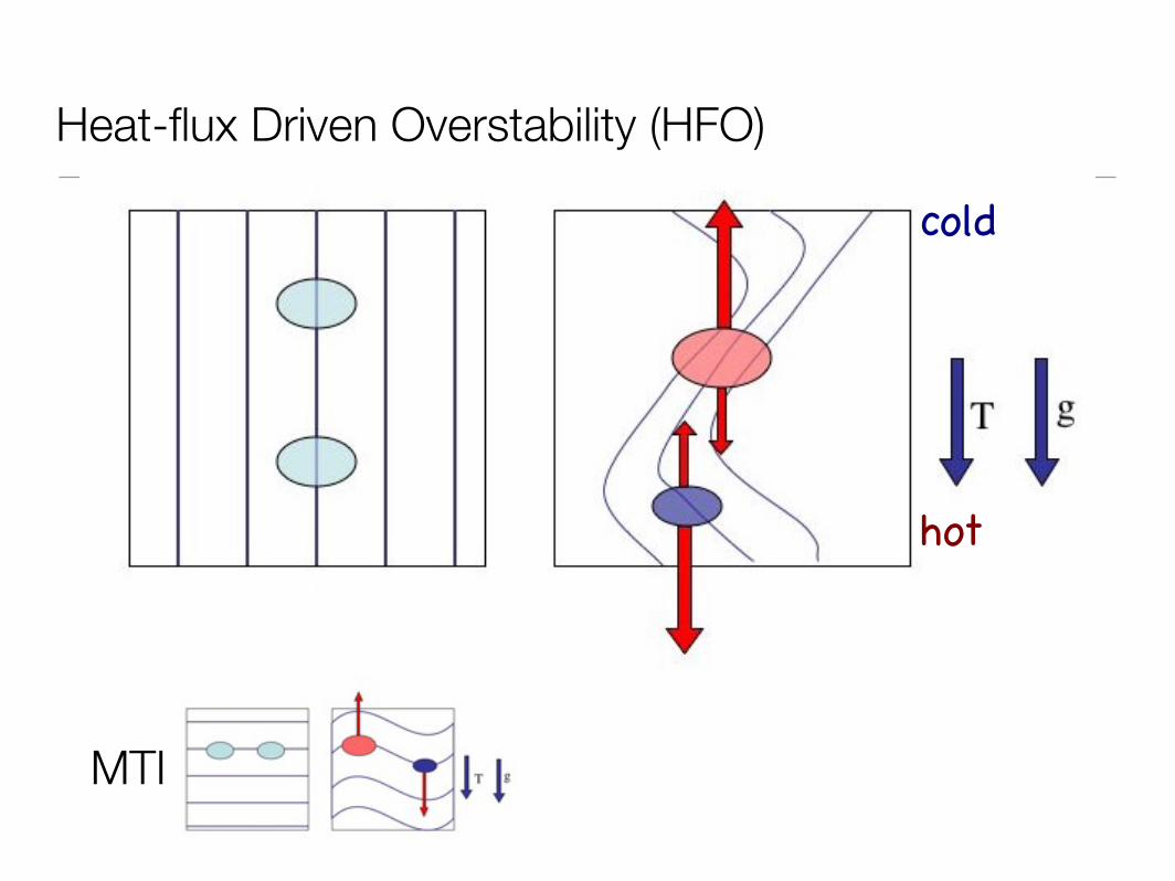
cold

hot

MTI

Heat-flux Driven Overstability (HFO)

T

hot

cold

g

Thermally unstable andoverstable to HFO

Thermally stable andoverstable to HFO

ωdyn ≳ ωcool > ωcondωdyn > ωcond

~2500 tdyn ~200 tdyn

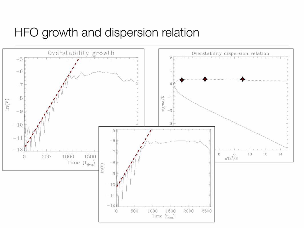
HFO growth and dispersion relation

Overstability driven by radiative cooling (RCO)

cold

hot

HBI

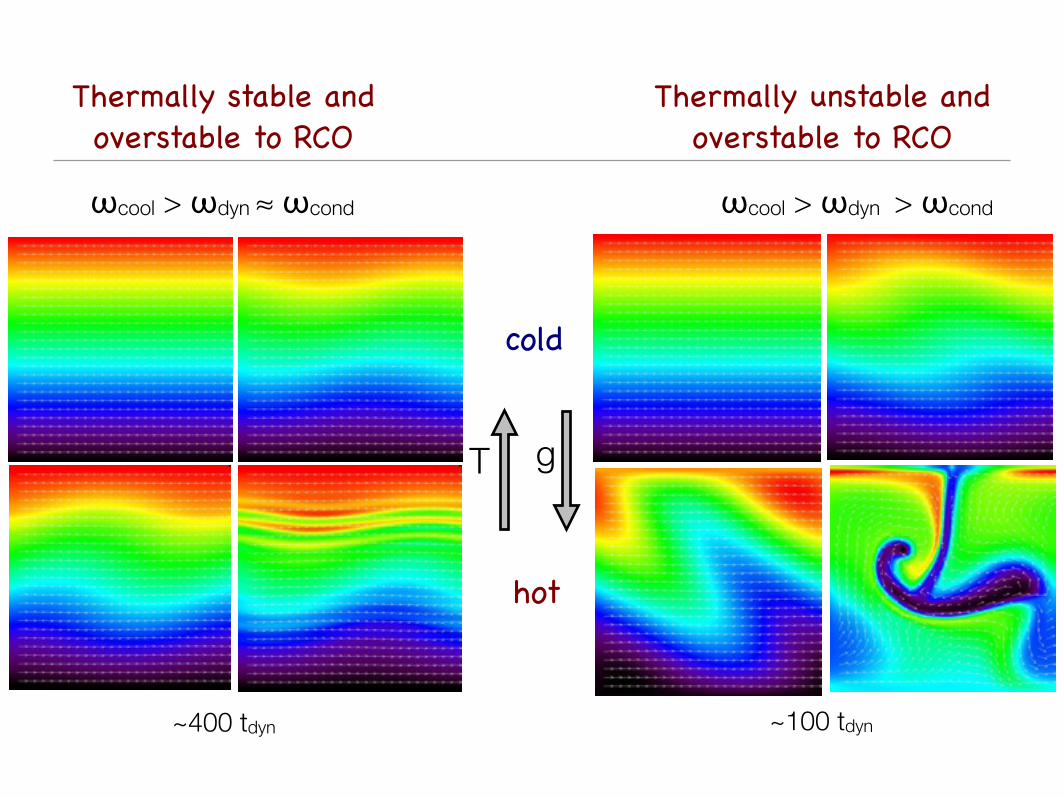
hot

cold

T g

Thermally unstable andoverstable to RCO

Thermally stable andoverstable to RCO

ωcool > ωdyn > ωcondωcool > ωdyn ≈ ωcond

~400 tdyn ~100 tdyn

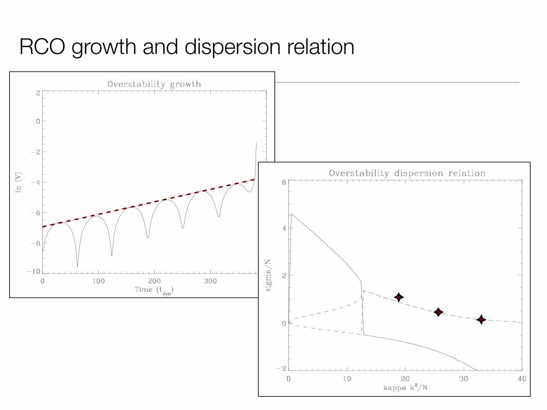
RCO growth and dispersion relation

Conclusions & prospects

• MHD overstabilities related to the well known MHD instabilities.

• Analytic theory: Need for thorough understanding of plasma processes (e.g., anisotropic viscosity).

• Simulations: Understanding the relative importance of individual plasma instabilities/overstabilities and their connection.

• Observations: Spectro-polarimetric measurements, measurements of temperature profiles and metallicity in cluster outskirts, measurements of turbulence, other yet to be realized methods...