Mechanics and Mechanical Engineering

Vol. 15, No. 4 (2011) 93–101

c⃝ Technical University of Lodz

Kinematics of a Robot with Crawler Drive

Krzysztof KurcDariusz Szybicki

Rzeszow University of TechnologyDepartment of Applied Mechanics and Robotics

kkurc@prz.edu.pldszybicki@prz.edu.pl

Received (15 December 2011)

Revised (16 January 2012)

Accepted (23 February 2012)

In this article authors presenting problems connected with the kinematics modeling mo-bile robot with crawler drive. This robot has been designed to enable monitoring andanalysis of the technical state of pipes and water tanks. Simulations of the kinematicsparameters have been made and the results are shown.

Keywords: Kinematics, modelling, mobile robot, crawler module

1. Introduction

In order to describe the kinematics of the robot with crawler drive it is necessaryto present kinematics equations. The problem of mathematical description of thekinematics equations of consideration to tracked skidding drive has been presented.In the MatlabTM–Simulink environment simulation of the robot’s kinematics be-haviour has been carried out. Such a mode of computations software have beenfurther discussed in paper [1,7,8]. On the basis of kinematics parameters simulationand comparison of the results have been carried out.

2. Kinematics description of the robot

On the crawler module track drive different types of variables interact over time.Description of crawler motion in real conditions, with the uneven ground with vari-able parameters, it is very complicated and therefore it is necessary to use simplifiedmodels [5, 6, 7, 8]. In addition to the widely-used crawler made ??up of cells, thereare also crawlers made up of an elastomeric belt. They constitute one elementwith the clutches (Fig. 1a). The propulsion system of the analyzed robot, the twomodules connected to the frame (Fig. 1b, Fig. 2).

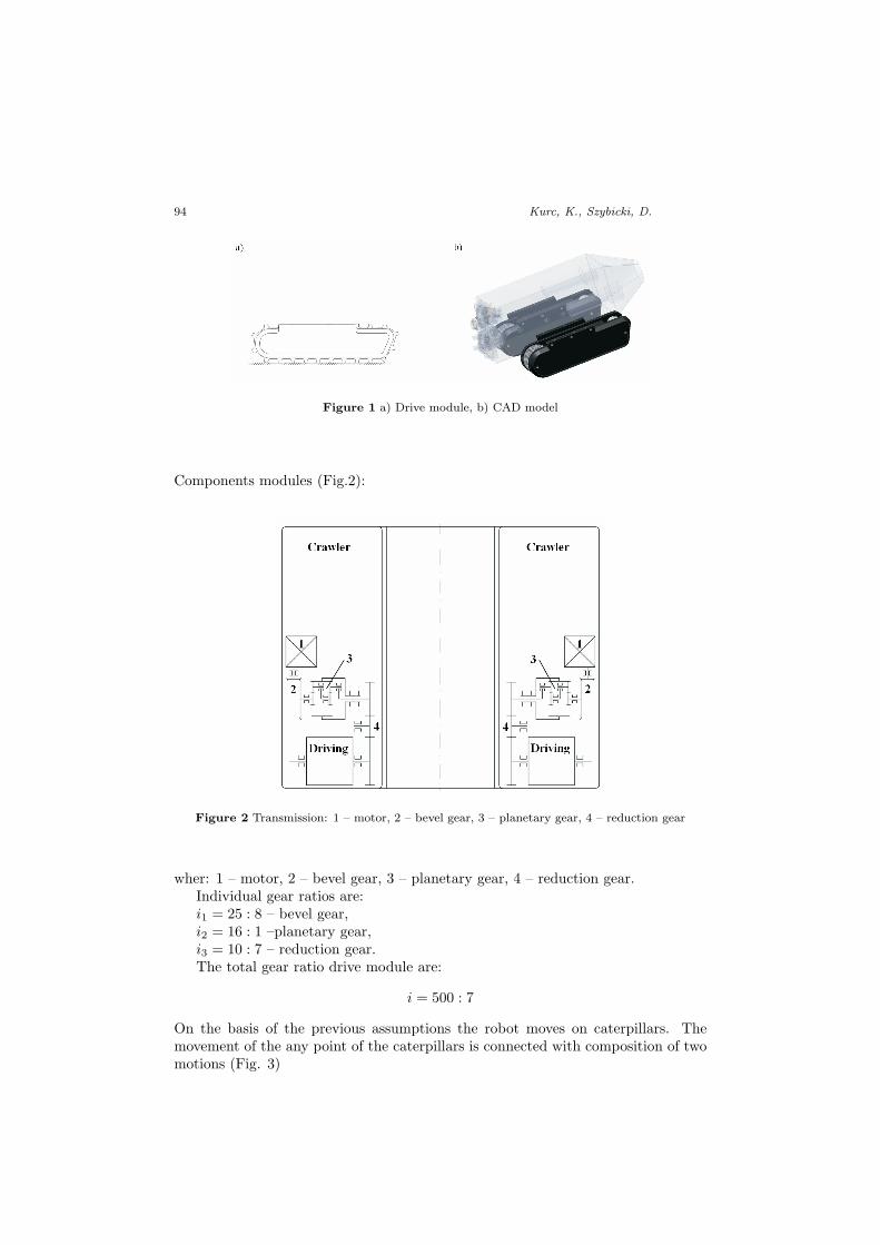
94 Kurc, K., Szybicki, D.

Figure 1 a) Drive module, b) CAD model

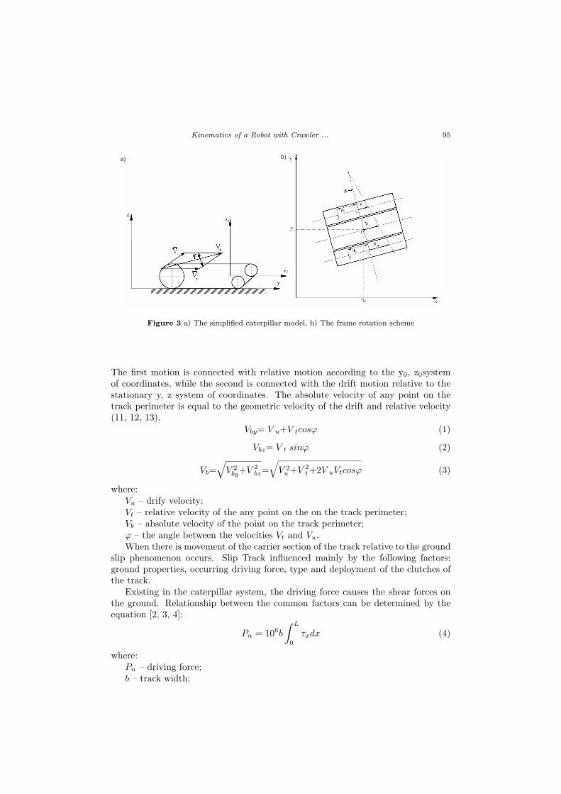
Components modules (Fig.2):

Figure 2 Transmission: 1 – motor, 2 – bevel gear, 3 – planetary gear, 4 – reduction gear

wher: 1 – motor, 2 – bevel gear, 3 – planetary gear, 4 – reduction gear.Individual gear ratios are:i1 = 25 : 8 – bevel gear,i2 = 16 : 1 –planetary gear,i3 = 10 : 7 – reduction gear.The total gear ratio drive module are:

i = 500 : 7

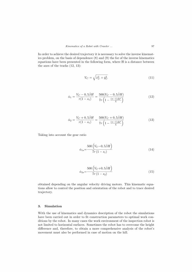
On the basis of the previous assumptions the robot moves on caterpillars. Themovement of the any point of the caterpillars is connected with composition of twomotions (Fig. 3)

Kinematics of a Robot with Crawler ... 95

a) b)

Figure 3 a) The simplified caterpillar model, b) The frame rotation scheme

The first motion is connected with relative motion according to the y0, z0systemof coordinates, while the second is connected with the drift motion relative to thestationary y, z system of coordinates. The absolute velocity of any point on thetrack perimeter is equal to the geometric velocity of the drift and relative velocity(11, 12, 13).

Vby= V u+V tcosφ (1)

Vbz= V t sinφ (2)

Vb=√V 2by+V 2

bz=

√V 2u+V 2

t+2V uVtcosφ (3)

where:Vu – drify velocity;Vt – relative velocity of the any point on the on the track perimeter;Vb – absolute velocity of the point on the track perimeter;φ – the angle between the velocities Vt and Vu.When there is movement of the carrier section of the track relative to the ground

slip phenomenon occurs. Slip Track influenced mainly by the following factors:ground properties, occurring driving force, type and deployment of the clutches ofthe track.

Existing in the caterpillar system, the driving force causes the shear forces onthe ground. Relationship between the common factors can be determined by theequation [2, 3, 4]:

Pn = 106b

∫ L

0

τxdx (4)

where:Pn – driving force;b – track width;

96 Kurc, K., Szybicki, D.

L – track carrier segment length;τx – shear stress in the soft ground.The maximum shear stress in the soft ground defines a Coulomb model [2, 3, 4]:

τmax = c+ µ0σ = c+ σtgρ (5)

where:ρ – internal friction angle of the ground particlesσ – compressive stresses in the groundµ0 – friction coefficient between the ground particles togetherc – density of the ground.The formula for the shear stress depends on the deformation, based on the

mathematical analogy between the course of the curves of shear stress and thecourse of the damped oscillation amplitude of the curve gave Bekker, they have theform(12, 13):

τx = (c+ σtgρ)e(−K2+

√K2

2−1)K1∆lx − e(−K2−√

K22−1)K1∆lx

Ymax[MPa] (6)

where:Ymax – The maximum value of the expression given in the numerator fraction∆lx – deformation of the ground layer at x, caused by slipping, parallel to the

groundK1 – coefficient of the ground deformation during the shearingK2 – coefficient characterizing the curve τ = f(s).Assuming that, in the course of deformation parallel to the ground is linear,

these deformation can be expressed by the formula:

∆lx = xsb (7)

where:sb – slip calculated from formulas (5) and (7);x – distance from the point for which the slip is calculated to the point of contact

with the ground of track, the largest slip occurs for x = L.On the bases of the description connected with the contact of the track with

the ground it is possible to describe the rotation of our robot in the x,y systemof coordinates, it is necessary to assume the characteristic point of the robot C.The scheme of robot motion has been presented in Fig.4. The velocity componentsof point C can be written as, after extension by angular velocity of the frame wereceive kinematics equations in the form with allow to solve forward kinematicsproblem:

xC =rα1(1− s1) + rα2(1− s2)

2cosβ (8)

yC =rα1(1− s1) + rα2(1− s2)

2sinβ (9)

β =rα2(1− s2)− rα1(1− s1)

H(10)

Kinematics of a Robot with Crawler ... 97

In order to achieve the desired trajectory it is necessary to solve the inverse kinemat-ics problem, on the basis of dependence (8) and (9) the for of the inverse kinematicsequations have been presented in the following form, where H is a distance betweenthe axes of the tracks (12, 13):

VC =√x2C + y2C (11)

α1 =VC − 0, 5βH

r(1− s1)=

500(VC − 0, 5βH)

7r(1− (n−1)∆l′

L

) (12)

α2 =VC + 0, 5βH

r(1− s1)=

500(VC + 0, 5βH)

7r(1− (n−1)∆l′

L

) (13)

Taking into account the gear ratio

α1s=500

(VC−0, 5βH

)7r (1− s1)

(14)

α2s=500

(VC+0, 5βH

)7r (1− s2)

(15)

obtained depending on the angular velocity driving motors. This kinematic equa-tions allow to control the position and orientation of the robot and to trace desiredtrajectory.

3. Simulation

With the use of kinematics and dynamics description of the robot the simulationshave been carried out in order to fit construction parameters to optimal work con-ditions by the robot. In many cases the work environment of the inspection robot isnot limited to horizontal surfaces. Sometimes the robot has to overcome the heightdifference and, therefore, to obtain a more comprehensive analysis of the robot’smovement must also be performed in case of motion on the hill.

98 Kurc, K., Szybicki, D.

ã

t=0-7[s]

t=13-20[s]

t=7-13[s]

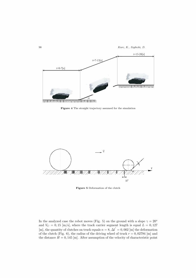
Figure 4 The straight trajectory assumed for the simulation

V

l"D

y

Figure 5 Deformation of the clutch

In the analyzed case the robot moves (Fig. 5) on the ground with a slope γ = 20o

and VC = 0, 15 [m/s], where the track carrier segment length is equal L = 0, 127

[m], the quantity of clutches on truck equals n = 8, ∆l′= 0, 002 [m] the deformation

of the clutch (Fig. 6), the radius of the driving wheel of truck r = 0, 02794 [m] andthe distance H = 0, 145 [m]. After assumption of the velocity of characteristic point

Kinematics of a Robot with Crawler ... 99

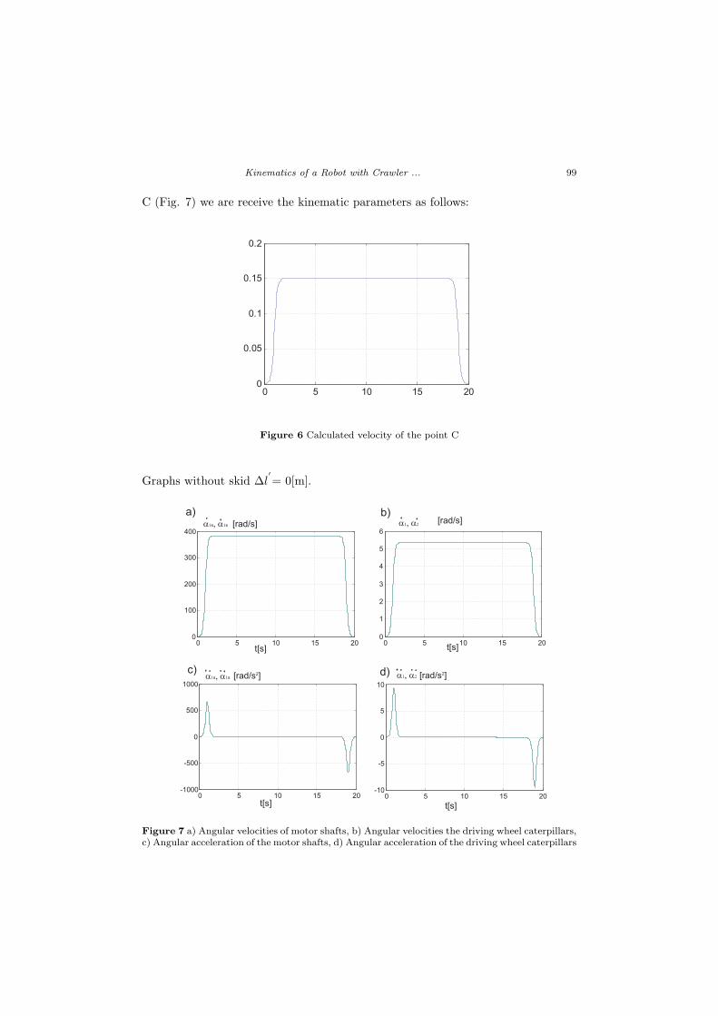
C (Fig. 7) we are receive the kinematic parameters as follows:

0 5 10 15 200

0.05

0.1

0.15

0.2

t [s]

Vc

[m/s

]

Figure 6 Calculated velocity of the point C

Graphs without skid ∆l′= 0[m].

0 5 10 15 200

100

200

300

400

0 5 10 15 200

1

2

3

4

5

6

0 5 10 15 20-1000

-500

0

500

1000

0 5 10 15 20-10

-5

0

5

10

a) b)

c) d)

t[s] t[s]

t[s] t[s]

a , a1 1s s

[rad/s] [rad/s]a , a1 1s s a , a1 2

a , a1 2[rad/s ]2 [rad/s ]2

Figure 7 a) Angular velocities of motor shafts, b) Angular velocities the driving wheel caterpillars,c) Angular acceleration of the motor shafts, d) Angular acceleration of the driving wheel caterpillars

100 Kurc, K., Szybicki, D.

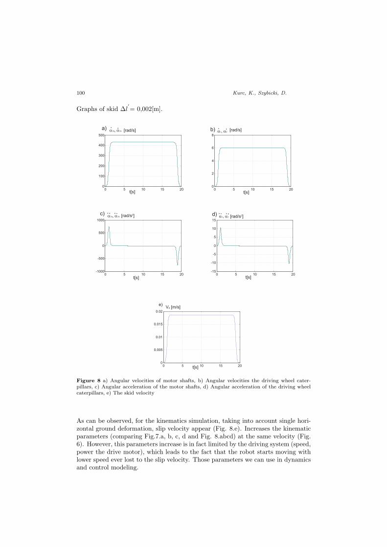
Graphs of skid ∆l′= 0,002[m].

0 5 10 15 200

100

200

300

400

500

0 5 10 15 200

2

4

6

8

0 5 10 15 20-1000

-500

0

500

1000

0 5 10 15 20-15

-10

-5

0

5

10

15

0 5 10 15 200

0.005

0.01

0.015

0.02

[rad/s]a , a1 1s sa) [rad/s]a , a1 2

a , a1 1s s [rad/s ]2a , a1 2 [rad/s ]2

b)

c) d)

t[s] t[s]

t[s] t[s]

t[s]

e)V [m/s]p

Figure 8 a) Angular velocities of motor shafts, b) Angular velocities the driving wheel cater-pillars, c) Angular acceleration of the motor shafts, d) Angular acceleration of the driving wheelcaterpillars, e) The skid velocity

As can be observed, for the kinematics simulation, taking into account single hori-zontal ground deformation, slip velocity appear (Fig. 8.e). Increases the kinematicparameters (comparing Fig.7.a, b, c, d and Fig. 8.abcd) at the same velocity (Fig.6). However, this parameters increase is in fact limited by the driving system (speed,power the drive motor), which leads to the fact that the robot starts moving withlower speed ever lost to the slip velocity. Those parameters we can use in dynamicsand control modeling.

Kinematics of a Robot with Crawler ... 101

4. Summary

The analysis of the kinematics and motion simulation takes into account factorsslipping track–dependent deformation of the substrate and claws. This approachwill be used for more detailed analysis taking into account additionally the turningof the robot on the hill. This will also be necessary during the identification andcontrol this type of object.

References

[1] Giergiel, J., Hendzel Z., Zylski, W. and Trojnacki, M.: Zastosowanie metod sz-tucznej inteligencji w mechatronicznym projektowaniu mobilnych robotow ko lowych,Krakow, 2004.

[2] Burdziski, Z.: Teoria ruchu pojazdu gasienicowego, Wydawnictwa Komunikacji i Lacznosci, Warszawa, 1972.

[3] Dajniak, H.: Ciagniki teoria ruchu i konstruowanie, Wydawnictwa Komunikacji i Lacznosci, Warszawa, 1985.

[4] Chodkowski, A. W.: Konstrukcja i obliczanie szybkobieznych pojazdowgasienicowych, Wydawnictwa Komunikacji i Lacznosci, Warszawa, 1990.

[5] Zylski, W.: Kinematyka i dynamika mobilnych robotow ko lowych, OficynaWydawnicza Politechniki Rzeszowskiej, Rzeszow, 1996.

[6] Trojnacki, M.: Modelowanie i symulacja ruchu mobilnego robota trzyko lowegoz napedem na przednie ko la z uwzglednieniem poslizgu ko ljezdnych, ModelowanieInzynierskie, Tom 10, No 41, p. 411–20, ISSN 1896–771X, Gliwice, 2011.

[7] Buratowski, T. and Giergiel, J.: Kinematics Modeling of the Amigobot Robot,Mechanics and Mechanical Engineering, International Journal, Vol. 14, No. 1, p.57–64,Technical University of Lodz, 2010.

[8] Giergiel, M., Hendzel Z. and Zylski W.: Modelowanie i sterowanie mobilnychrobotow ko lowych, PWN, Warszawa, 2002.