kinematic and dynamic approaches in gait optimization for

Kinematic and Dynamic Approaches in GaitOptimization for Humanoid Robot Locomotion

Ramil Khusainov1, Alexandr Klimchik1(B), and Evgeni Magid2

1 Intelligent Robotic Systems Laboratory, Innopolis University, Innopolis City,Russian Federation

[email protected], [email protected] Higher Institute of Information Technology & Information Systems, Kazan Federal

University, Kazan, Russian [email protected]

Abstract. Humanoid robot related research keeps attracting manyresearchers nowadays because of a high potential of bipedal locomotion.While many researchers concentrate on a robot body movement due toits direct contribution to the robot dynamics, the optimality of a legtrajectory has not been studied in details yet. Our paper is targeted todecrease this obvious gap and deals with optimal trajectory planning forbipedal humanoid robot walking. The main attention is paid to maxi-mization of locomotion speed while considering velocity, acceleration andpower limitations of each joint. The kinematic and dynamic approachesare used to obtain a desired optimal trajectory. Obtained results providehigher robot performance comparing to commonly used trajectories forcontrol bipedal robots.

Keywords: Humanoids · Bipedal walking · Optimal trajectory plan-ning

1 Introduction

Nowadays one of the most challenging tasks in robotics is developing multi-purpose terrain robot which could perform various tasks, including operationsin difficult and dangerous conditions. Such operations may require humanlikeskills to overcome obstacles and get through environment, which was originallydesigned for a human. That is why it is critically important to develop humanoidrobots, which are similar to human body in their size, weight and locomotioncharacteristics. Many theoretical and experimental researches have been donein the field of biped robots during three past decades and many notable devel-opments have been achieved [1]. There are various practically realized systems,from the simplest cases of planar robots, to the most advanced robots, withmany Degrees of Freedom (DoF) [2–4].

However, we are still very far from widespread use of humanoids. Mainlythis is because biped robots’ poor locomotion abilities and its ability to fall

c© Springer International Publishing AG 2018K. Madani et al. (eds.), Informatics in Control, Automation and Robotics,Lecture Notes in Electrical Engineering 430, https://doi.org/10.1007/978-3-319-55011-4_15

294 R. Khusainov et al.

down. Although there are some efficient algorithms for the several applicationareas of humanoid robots [5], but it is very difficult to merge all of them intoone efficient system because the overall system’s complexity becomes extremelyhigh. Especially the problem manifests itself when robot moves on rough terrain,steep stairs, and in environments with obstacles. Hence, robot stability relatedresearch keeps attracting many researchers nowadays in order to propose goodrobot locomotion control algorithms and to prevent a biped robot from fallingdown.

Walking stability can be divided into static and dynamic. The static stabilitycan be verified through being the center of gravity (COG) in the stability area(supporting polygon). There are several stability criteria for biped walking butmostly the dynamic stability is verified via Zero Moment Point (ZMP) criterion[6]. ZMP is a point on the ground at which the total moments due to groundreaction force becomes zero. In other words, the influence of all ground forcescan be replaced by one force applied in ZMP point. In order to achieve a dynam-ically stable gait the ZMP should be within the support polygon, at every timeinstance. The assumption of ZMP approach is that dynamic biped walking canbe decomposed into two parts, a walking pattern generation and a stabilizationaround it. In this paper we discuss the first part. The research studies on walk-ing gate generation can be classified into three main groups, i.e. robot modeling,walking pattern generation and gait parameter optimization.

Robot modeling works on reducing complexity of robot motion dynamicswith certain approximation error. Here compromise is required between modelerror and computational cost. In many research studies inverted pendulum model(IPM) utilized, which approximates robot as a single point mass concentratedat the center of mass (COM) [7]. The model is simple but leads to significantZMP error since usually legs of the robot are heavy and cannot be neglected. Analternative here is utilization multiple masses IPM (MMIPM) model robot [8],which consists multiple point masses. To make model effective it is required tochoose proper number of point masses to ensure optimality from cost/error pointof view. Sato et al. [9] proposed three mass IPM (3MIPM) with point massesat COM and feet, Ha and Choi [10] proposed virtual height IPM (VHIPM)that has dynamics form of IPM for multiple mass model. In practice, modelchoice highly depends on the gait generation and control methods. There aretwo main approaches to generate walking pattern: using online or/and offlinemethods. In online methods, computational cost is the main issue and full bodydynamics cannot be processed. Therefore, simplified methods are used. In offlinepath planning we can calculate full or almost full body dynamics that gives moreaccuracy for humanoid locomotion.

As it was already mentioned, in order to keep robot stable during locomotionwe should generate such trajectory that keeps ZMP point inside of supportingpolygon. Several techniques for generating walking motion for biped robots wereproposed in the literature. For instance, in [11] polynomial trajectories were used,in [7] authors employed Fourier series. Katoh and Mori [12] demonstrated thatusing a Van der Pol oscillator as generator of the tracking reference would induce

Kinematic and Dynamic Approaches . . . 295

walking trajectories for a biped robot. Furusho and Masubuchi [13] presented thewalking control algorithms by tracking a piecewise-linear joint reference trajec-tory. Another method for trajectory generation is to mimic the human rhythmicfunction by means of a central pattern generator, just as it is reported in [14].Kajita in [15] proposes ZMP tracking servo controller which adopts the previewcontrol theory [16] that uses the future ZMP reference.

Gait parameter optimization is another important issue. It is importantto decide optimal foot placements, CoM trajectory or walking speed consid-ering constraints in joint actuators and energy efficiency. Goswami et al. appliedgenetic algorithm (GA) to maximize ZMP stability and step length by optimizingfour gait parameters [17]. In addition, Dau et al. [18] planned foot and hip trajec-tories using polynomial interpolation and used GA to minimize the mechanicalenergy by optimizing the seven key parameters for the hip and foot trajectories.Liu et al. [19] designed ZMP trajectory to minimize an energy related functionusing fuzzy logic. In [20] authors applied dynamic programming approach tooptimize walking primitives considering kinematic limits only.

Compared with previous works, our main problem was to estimate maxi-mum walking speed, that can be achieved with given humanoid robot underactuator power and joint limit constraints. We used two approaches to solvethe problem. The first, kinematic approach, operates only with robot kinematicsand uses maximum joint velocities and accelerations. In dynamic approach wesolved optimization problem with seven key walking parameters and with fullbody dynamics calculation.

The reminder of the paper is organized as follows. In Sect. 2 we formulate theproblem. Section 3 focuses on kinematic approach in gait optimization. Section 4presents dynamic approach for optimization problem. Finally, conclusions aredrawn in Sect. 5.

2 Problem Statement

Majority of the algorithms for stable walking of a bipedal robot usually focuson balance control and do not take into account joint constraints. There-fore, calculated trajectories may be not reachable in practice because of veloc-ity/acceleration/jerk limits in joints and lead to wrong foot positioning. On theother hand, there are works which study trajectory optimality with joints limits,but without stability analysis of such trajectories.

Anthropomorphic robot AR-601M [21] (Fig. 1), which is in the focus of ourstudy, has 41 DoF in total, although during walking only 12 joints are used (6 ineach pedipulator). For simplicity, we take into account that the robot motionlies in a sagittal plane. In this case, the problem of optimal trajectory can bereduced to the 5 DoF system.

The problem, which we analyse in our research can be formulated as follow-ing: find the optimal parameters of repeating steps motion such as step length,step time, hip height and etc., that maximize walking speed under robot con-straints.


Fig. 1. Anthropomorphic robot AR-601M and its 5 DoF model in sagittal plane

3 Kinematic Approach

3.1 Dynamic Programming Method for Swing Leg TrajectoryOptimization

In this approach the optimal trajectory problem does not consider trunk motionand can be is reduced to 2DoF system. Thus, the swing leg could be representedas a simple two-link system with hip and knee joints. The corresponding toAR601-M robot leg parameters link lengths are equal to 280 mm each. Since inour models robot body moves at a constant speed, for simplicity, its movementis ignored and we assume a fixed position of the hip joint. This means thatconsidered problem is represented in a moving coordinate system. The trajectoryof the swing leg and principle model parameters are shown in Fig. 1.

Optimization Criteria

There are different approaches to define cost function in optimal trajectorysearch problem. For example, Nakamura et.al. in [22] minimized energy con-sumption, which can be written in the form:

2∑

i=1

[τiθi + γτ2

i

]dt (1)

where τi is joint i torque, θi is joint i velocity, γ is an empirical constant. Thefirst term in (1) corresponds to mechanical work, which is performed to movedynamic system. The second term corresponds to heat emission in each jointdue to torque generation. It was shown, that optimal trajectory which could befound in such a way well agrees with experimental data of human locomotion.Yet, while obtaining a swing leg trajectory, the authors do not take into accountmaximum joint velocity and acceleration limitations, which actually provide crit-ical constraints for a real robot. A selected trajectory could be energy optimal


in theory, but if the robot’s motors could not supply required by such trajectorytorques, the physical robot will fail to perform such trajectory [23].

In practice, walking speed is one of the most important performance mea-sures for bipedal robots. Walking speed could be unambiguously calculated, whileenergy consumption calculation is not that obvious as it depends on many fac-tors; e.g., energy is mainly consumed in supporting leg joints, since they havemuch higher actuating torques than swing leg joints (in our work only swing legmotion is considered). In addition, energy consumption strongly correlates withstep time: the faster a swing leg moves for a given step length, the lower is itsenergy consumption. Therefore, minimization of each step time is a critical issueto be considered, and it is the core contribution of our paper. Step time can beevaluated as

t =∫

S

(1/V ) dS (2)

where V is a foot speed in Cartesian space and dS is the foot path. Time t iscalculated numerically by dividing the trajectory into a finite number of intervalsand further summing up over all intervals.

Search Algorithm.

Different techniques can be used to find swing leg optimal path of bipedal robot.For example, spline genetic algorithm (GA) in [22] determined a joint torquefor several trajectory points and interpolated it for other points using thirdorder spline. A significant drawback of this method is the GA algorithms featureof finding a global minimum for continues functions. A heuristic optimizationmethod was used in [24] to find optimal trajectory with Harmony Search algo-rithm for 6 DoF manipulator. Smooth trajectories that comply kinematic con-straints (velocity and acceleration) were obtained, but only 6 via-points betweenstart and end points were used.

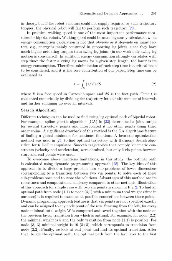
To overcome above mentions limitations, in this study, the optimal pathis calculated using dynamic programming approach [25]. The key idea of thisapproach is to divide a large problem into sub-problems of lower dimensionscorresponding to a transition between two via points, to solve each of thesesub-problems once and to store the solutions. Advantages of this method are itsrobustness and computational efficiency compared to other methods. Illustrationof this approach for simple case with two via points is shown in Fig. 2. To find anoptimal path from node (1,1) to node (4,1) with a minimum total weight (time inour case) it is required to examine all possible connections between these points.Dynamic programing approach feature is that via points are not specified exactlyand can be assigned to any node point of the row. Starting from the left, for everynode minimal total weight W is computed and saved together with the node onthe previous layer, transition from which is optimal. For example, for node (2,2)the minimal weight is 5 and the only transition from node (1,1) is possible. Fornode (3, 3) minimal weight is 10 (5+5), which corresponds to transition fromnode (2,2). Finally, we look at end point and find its optimal transition. Afterthat, to get the optimal path, the optimal path from the last layer to the first


Fig. 2. Example of directed graph and building directed graph in search area by cre-ating 2D grid

layer is constructed. For the provided example the optimal path corresponds tothe following path: (4,1), (3,3), (2,2), (1,1).

To transform optimal path search problem for a bipedal robot into a directedgraph it is required to put evenly distributed nodes pi,j within the search space,which covers all possible trajectory paths. Here it is required to create a twodimensional grid with nx+1 points in x direction and ny +1 points in y direction(see Fig. 2). Since we consider the trajectories with certain height limit ymax andstep length xmax the desired search space size is equal to xmax×ymax area, whichcontains nx − 1 via points to be assigned.

The algorithm for finding the optimal path works as follows:

• For each node point pi,j , i = 1, j = 1, ny + 1 calculate the weight (i.e., thecost), which corresponds to the transition minimum time to that node fromthe start point p0,0. In each node save the weight and joints angular velocitiesat the end of the corresponding trajectory.

• For each node pi,j where i = 2, nx, j = 1, ny + 1 calculate the weight oftransition from pi−1,k node, where k = 0, ny + 1. Find kmin, for which thesum of the calculated weight for transition from pi,kmin and total weight ofpi,kmin node is minimal. In each node pi,j save kmin, the total weight and jointsangular velocities, which are calculated for the transition from pi,kminto pi,j .

• For node pnx+1,0 (end point) calculate the weight of the transition from pnx,k,where k = 0, ny + 1. Find kmin, for which the sum of the calculated weightand the total weight of pnx,kmin

node is minimal.

• Obtain an optimal trajectory by tracking backward kmin values for each node:

pnx+1,ny+1 → pnx,knx+1min

→ pnx−1,knxmin

→ . . . → p1,k2min

→ p0,0

where knx+1min is the optimal track for pnx+1,ny+1node.

Since the transition time between two node points is used as a cost function,it is required to calculate minimal traveling time from node pi−1,k to node pi,j


taking into account velocity and acceleration limits. First of all, joint anglesincrements are calculated for each transition between two adjacent nodes. Thenmark a joint as active if it has larger absolute value of angular increment for agiven transition. Without loss of generality let’s assume that joint 1 is active andjoint 2 is passive. Assuming that active joint for each interval move either witha constant speed or a constant acceleration (depending whether it reaches themaximum velocity on previous interval), the joint movements can be describedas follows

Δϕ(i) = ω(i)s t + 0.5a(i)t2 (3)

ω(i)e = ω

(i)s + a(i)t (4)

where i=1 for an active joint and i=2 for a passive joint, Δϕ is an angularincrement,ωs and ωe are angular velocities at start and end of the interval respec-tively, a is an angular acceleration and t is a transition time.

In order to describe all possible relations between active joints on the adja-cent intervals, three different cases for calculating transition time should beconsidered:

Case 1: Maximum Velocity. If an absolute angular velocity of an active jointin pi−1,k node is equal to the maximum value ωmax and its sign is equal tothe sign of angular increment Δϕ, then t =

∣∣Δϕ(1)∣∣ /ωmax, a(1) = 0, ω

(1)e =

ω(1)s . Substituting t into equations (3) and (4) we obtain a(2), ω

(2)e . It should be

emphasized that if the sign of angular increment Δϕ is opposite to the currentvelocity sign at the beginning of interval than either Case 2 or Case 3 should beconsidered.

Case 2: Maximum Acceleration. If an absolute angular velocity of an activejoint in pi−1,k node is below its maximum value ωmax or its sign is opposite tothe sign of angular increment Δϕ, then we substitute Δϕ(1) into equation (3)with a(1) = sign(Δϕ(1))amax and solve the second order equation with respectto t:

t =−w

(1)s ±

√(w(1)

s )2 + 2a(1)Δϕ(1)

a(1). (5)

Next, we select the lower positive root of the above equation and calculate ω(1)e =

ω(1)s + a(1)t. If

∣∣∣ω(1)e

∣∣∣ is less than or equal to ωmax, than a(1)and ω(1)e are equal

to the calculated values. Finally, we substitute t into Eqs. (3)–(4) to obtain a(2),ω(2)e .

Case 3: Reaching Maximum Velocity. If Case 1 condition is not satisfiedand

∣∣∣ω(1)e

∣∣∣in Case 2 is greater than ωmax, than ω(1)e = sign(Δϕ(1))ωmax, t =

2Δϕ(1)/(ω(1)e + ω

(1)s ), a(1) = (ω(1)

e − ω(1)s )/t. We substitute t into Eqs. (3)–(4)

to obtain a(2), ω(2)e . Figure 3 demonstrates all three cases which are described


Fig. 3. Three cases of angular velocity behaviour: (1 ) maximum velocity; (2 ) maximumacceleration; (3 ) reaching maximum velocity

above. For all cases we verify if the calculated joint angular accelerations andvelocities are below their maximal values. If this condition cannot be satisfied,this transition is excluded from a possible path of the swing leg.

Optimization Results.

The simulation of the algorithm was performed within MATLAB/Simulink envi-ronment. The acceleration and velocity limits were assigned to 1 rad/s2 and1 rad/s respectively for each joint. First, let us obtain optimal walking primi-tives for the fixed hip rising height and step length and then compare resultswith optimal parameters settings.

For the first case hip height was fixed to 0.5 m in order to ensure optimallocomotion speed of the robot based on our previous empirical studies [23,26].According to joint limits and link parameters we selected the robot step length tobe 0.4 m. For these parameters hip and knee joint angles in their starting positionwere set to 0.1 and 0.55 rad correspondingly; at the end of the trajectory (goalposition) hip and knee joint angles were set to –0.66 and 0.55 rad correspondingly.These angles define pi,j and pi,j nodes.

Next, three different cases were analyzed:

(i) movement without any trajectory constraints, i.e. in an ideal case withoutvelocity/acceleration limits the foot may move straightforwardly from astart point to an end point (Fig. 4 left);

(ii) movement with 0.1 m barrier (with negligible small size in the robot walkingdirection) in the middle of the trajectory (Fig. 4 right);

(iii) movement with 0.05 × 0.2 m box barrier in the middle (Fig. 5).

The results demonstrated that for all cases the obtained Cartesian trajec-tories of a swing leg do not correspond to the shortest path and differ from acycloid path, which is traditionally used in bipedal robot locomotion control. Tocompare our results with a cycloid path approach, we built the cycloid trajectoryfor (ii) case and ensured the same travelling time as for our optimal trajectory(Fig. 4a right). The corresponding angular velocities are presented in Fig. 6. Thesimulation demonstrated that for the cycloid trajectory, the knee angular veloc-ity exceeds maximum value and the accelerations at the beginning and at theend of the trajectory are very high. That means that in practice it is impossible


Fig. 4. Optimal trajectory without obstacles for hip height 0.5 m and step length 0.4 m(left) and trajectories with 0.1 m barrier in the middle for hip height 0.5 m and steplength 0.4 m (right): a foot trajectory in Cartesian space; b angular velocity of joints;c angular acceleration of joints

to perform such trajectory within the specified time. In order to move along acycloid trajectory, it is required to scale (increase) travelling time according tothe velocity limits. Hence, the proposed algorithm succeeds to suggest a foottrajectory with a shorter time interval comparing to a typical cycloid trajectory.

In the case without trajectory constraints, the foot rises up to 0.04 m, which iscaused by joint velocity/acceleration limits. It is evident that travel time in suchcase is minimum. The particularity of this trajectory is that the joint velocitylimits are not reached (see Fig. 4b left).

Barrier profile essentially effects optimal trajectory (see Figs. 4a and 5a).Although the (ii) case barrier is two times lower than for case (iii), the height ofthe optimal trajectory for case (iii) and its travel time are higher.

To compare efficiency of the obtained walking primitives with conventionalcycloids, the joint speed and acceleration profiles have been obtained for cycloidsas well. It should be stressed, that these profiles do not satisfy velocity andacceleration limits, and to ensure such trajectory implementation it is requiredto increase traveling time. In particular, for free motions without obstacles theacceleration limits have been exceeded by the factor 6, and to remain within


Fig. 5. Optimal trajectory with 0.05 × 0.2 m box barrier in the middle for hip height0.5 m and step length 0.4 m: a optimal foot trajectory in Cartesian space; b angularvelocity of joints; c angular acceleration of joints

Fig. 6. Angular velocities of joints for cycloid trajectory movement with 0.1 m barrier,case of for hip height 0.5 m and step length 0.4 m


Fig. 7. Robot AR601M speed map for different step length and hip height for thetrajectory without obstacles

Fig. 8. Robot AR601M speed map for different step length and hip height for thetrajectory with 0.1 m barrier in the middle

the limits traveling time should be over 10 s, which is twice higher that forthe obtained optimal trajectory. Another limitation of conventional trajectoryplanning approach is its sensitivity to a swing height and request to providetraveling time as an input parameter. Our proposed approach does not havethese limitations and automatically estimates minimal traveling time and anoptimal swing leg height.

Now, let us obtain optimal hip heights and step length for all cases consideredabove and compare robot performance. Speed maps for different step length andhip height are presented in Figs. 7, 8 and 9. Here, lighter colour corresponds tohigher speed and are preferable for robot locomotion. It is shown that Cartesianspeed highly depends on the step length and hip height and varies from one caseto another. It is also shown that optimal step parameters highly depend on thesize of the obstacle, which appears on the robot path. In particular, for the casewithout obstacles optimal settings are hip height of 0.4 m and step length of0.32 m, while for the case of box barrier the optimal step length is much higher(0.52 m) and hip height is almost the same (0.45 m).


Fig. 9. Robot AR601M speed map for different step length and hip height for thetrajectory with 0.05 × 0.2 m box barrier in the middle

Table 1. Optimal walking parameters for locomotion of bipedal humanoid robot AR-601M

Case Step length(m)

Hip height(m)

Speed (m/s)

Fixed param.a Optimalparam.b

(i) withoutobstacles

0.32 0.40 0.13 0.16

(ii) with 0.1 mbarrier

0.56 0.43 0.09 0.12

(iii) with 0.05× 0.2 m boxbarrier

0.52 0.45 0.11 0.12

aFixed hip and step length parameters are 0.5 and 0.4 m respectivelybOptimal hip height and step length parameters

Optimisation results are summarised in Table 1. Optimal walking parametersfor locomotion of bipedal humanoid robot AR-601M, where for the three casesan optimal hip height, a step length and a corresponding robot speed are given.For comparison purposes it also contains robot speed for the case of a fixed hipheight and step length studied above. It is shown that for the case of optimalhip and step size parameters robot speed increases by 10–23%, depending howfar initial parameters were from the optimal ones.

For comparison purposes Fig. 10. Optimal trajectory without obstacles for0.4 m hip height and 0.32 m step length: (a) foot trajectory in Cartesian space;(b) angular velocity of joints; (c) angular acceleration of joints contain walkingprimitives with joint velocities and accelerations for motion without obstacles.


0 0.5 1 1.5 2-1

0

1

hip knee

0 0.05 0.1 0.15 0.2 0.25 0.3 0.350

2

4

610 -3

0 0.5 1 1.5 2-1

-0.5

0

0.5 hipknee

,y m

, /rad sω

,x m

,t s

,t s

2, /a rad s

(a)

(b)

(c)

Fig. 10. Optimal trajectory without obstacles for 0.4 m hip height and 0.32 m steplength: a foot trajectory in Cartesian space; b angular velocity of joints; c angularacceleration of joints

A rather evident fact that for an optimal robot speed without no obsta-cles, an optimal trajectory should be close to the ground level was confirmed bysimulation results. It is clear that in practice such trajectory could be hardlyimplemented (in fact, it is not possible to have zero step height while loco-motion), while it demonstrates efficiency of the proposed approach. With suchmoving primitive the robot can move with 0.16 m/s velocity instead of 0.13 thatis maximal for 0.5 m hip height and 0.4 m step length. Similar tendencies areobserved for all considered cases.

Advantages and Limitations.

In spite of numerous advantages, the proposed walking trajectory optimizationapproach has several apparent limitations, and the most significant one amongthem is ignoring of dynamic and static effects within optimization procedure. Infact, static effects (compliance errors) are not critical for the trajectory optimiza-tion since they are relatively small and could be easily compensated by integrat-ing a feedback control from the feet force sensors. In this case the main limitation


for the moving primitive is avoiding joint coordinates limits, which may not allowthe robot to compensate induced compliance errors. From another side, if feed-back control is not available compliance errors should be computed using linearor non-linear stiffness modelling [27,28] and control algorithm should rely on theelasto-geometric model [29,30]. It should be stressed that stiffness parameters forreal robot can be obtained from the dedicated experimental study only [31]. So,statics effects the control algorithm, but is not critical for optimization walkingprimitives.

On the other side dynamic effects directly influence robot stability [32,33]and can be hardly compensated, since this will directly affect walking primitiveprofile. Since walking profile contains only foot coordinate, humanoid torso andarms could be used to additionally increase robot balance [34,35]. From anotherside, integrating dynamic model into optimization procedure may provide addi-tional tool for trajectory optimization. It may lead to faster robot movements inthe case when joint acceleration will be induced not only because of actuationforces, but also by dynamic forces. However, this approach essentially compli-cates computations and may be hardly implemented for robot control throughjoint angles instead of demanded force level control. Besides, swing leg does notcontribute a lot in robot dynamics since it does not effect robot body motion,which mostly defining robot stability. In contrast, it is a supporting that mainlydefines CoM trajectory and, consequently, robot stability. From that point ofview supporting leg trajectory could be unambiguously determined from sta-bility condition while swing leg coordinates are redundant variables that mightbe optimised while step trajectory planning is proposed in this work. So, thesuggested approach is a trade-off between a model complexity and utilization ofrobot total capacities. In practice, to avoid unpredictable robot behaviour, it isreasonable not to use upper velocity/acceleration boundaries in the optimiza-tion procedure since they may be higher in real model because of a presence ofdynamic forces and errors in the model parameters.

The most essential limitation of the provided results is related to kinematicconstraints induced to a hip location. It was strictly assumed that the hip heightremains the same along the trajectory, while it is obvious that the best robotspeed will be achieved when the height varies along the trajectory. In our app-roach, we separate swing and supporting leg movements and consider only aswing leg trajectory. Since a swing leg travels longer distances in walking, itsjoints should apply higher speeds and accelerations. Therefore, optimality due tokinematic limits is more important for a swing leg. We consider swing leg move-ment in coordinate system of a hip where the hip is fixed. Another direction forenhancing optimization efficiency is considering hip speed as an additional opti-mization parameter, which may vary from one via point to another. Providingreasonable solutions of the above-mentioned drawbacks and their integrationinto the optimization algorithm will apparently lead to robot speed increase.These issues will be addressed in details in our future work.


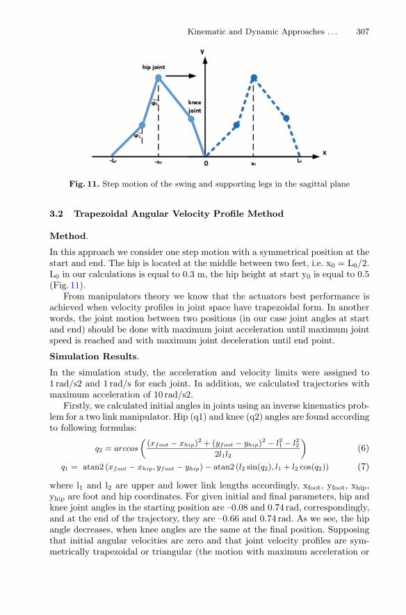
Fig. 11. Step motion of the swing and supporting legs in the sagittal plane

3.2 Trapezoidal Angular Velocity Profile Method

Method.

In this approach we consider one step motion with a symmetrical position at thestart and end. The hip is located at the middle between two feet, i.e. x0 = L0/2.L0 in our calculations is equal to 0.3 m, the hip height at start y0 is equal to 0.5(Fig. 11).

From manipulators theory we know that the actuators best performance isachieved when velocity profiles in joint space have trapezoidal form. In anotherwords, the joint motion between two positions (in our case joint angles at startand end) should be done with maximum joint acceleration until maximum jointspeed is reached and with maximum joint deceleration until end point.

Simulation Results.

In the simulation study, the acceleration and velocity limits were assigned to1 rad/s2 and 1 rad/s for each joint. In addition, we calculated trajectories withmaximum acceleration of 10 rad/s2.

Firstly, we calculated initial angles in joints using an inverse kinematics prob-lem for a two link manipulator. Hip (q1) and knee (q2) angles are found accordingto following formulas:

q2 = arccos

((xfoot − xhip)

2 + (yfoot − yhip)2 − l21 − l22

2l1l2

)(6)

q1 = atan2 (xfoot − xhip, yfoot − yhip) − atan2 (l2 sin(q2), l1 + l2 cos(q2)) (7)

where l1 and l2 are upper and lower link lengths accordingly, xfoot, yfoot, xhip,yhip are foot and hip coordinates. For given initial and final parameters, hip andknee joint angles in the starting position are –0.08 and 0.74 rad, correspondingly,and at the end of the trajectory, they are –0.66 and 0.74 rad. As we see, the hipangle decreases, when knee angles are the same at the final position. Supposingthat initial angular velocities are zero and that joint velocity profiles are sym-metrically trapezoidal or triangular (the motion with maximum acceleration or


Fig. 12. Angular velocity profiles and joint angle profiles of the swing leg. A triangularcase

Fig. 13. Angular velocity profiles and joint angle profiles of the swing leg. A trapezoidalcase

speed), we can find the time needed for hip joint angle change. After that, forthe given time we define a velocity profile for the knee joint, again taking intoconsideration zero initial and final velocities, a symmetrical trapezoidal or tri-angular function with a total zero integral (angle change). Joint angle functionsare found from velocity functions by integration with known initial values. Fig-ures 12 and 13 show velocity and angle functions for acceleration limits 1 and10 rad/s2 correspondingly. The motion time is 1.53 s for lower and 0.68 s forhigher acceleration. We see that in the first case, the maximum velocities arenot reached, when in the second case, profiles are trapezoidal. Since the motionis symmetrical, which means that final angles of the swing leg are initial anglesof the supporting foot, we define velocity profiles of the supporting leg as profilesof the swing leg with an opposite sign.

After joint angle functions are found, we use the forward kinematics solutionto find the foot trajectory in Cartesian space. Figure 14 shows foot trajectoriesfor two acceleration limits. We see that in both cases, the foot is always abovethe ground, which is a necessary requirement.

However, the stability analysis of such trajectories shows that this kind ofmotion is unstable if there is no additional compensation of ZMP deviation fromthe stable one, corresponding to the center of the supporting foot. Therefore,such optimal trajectories are applicable only if we use the upper body motionto balance the robot dynamics during walking.


Fig. 14. The trajectory of the swing foot in Cartesian space for the lower (left) andhigher (right) acceleration limit

Fig. 15. Model of biped robot with 5 DoF and 5 links and Stick diagram of half walkingcycle

4 Dynamic Approach

In dynamic approach the optimization problem is solved for 5 link model shownin Fig. 15. Model has 5 DoF and similar to kinematic approach considered abovefor 2D motion in sagittal plane. Length, mass and moment of inertia parametersof links are given in Table 2. These parameters correspond to the characteristicsof AR601M.

Table 2. Manipulator link parameters

Link L (m) d (m) Mass (kg) Moment ofinertia (kg*m2)

Trunk 0.65 0.3 44.8 0.72

Thigh 0.28 0.14 6.8 0.055

Shank 0.28 0.12 3.9 0.038


Dynamic approach for searching optimal motion trajectory can be dividedinto following steps:

1. Parametrization of walking gait2. Calculation of joint torques and velocities that ensure given trajectories3. Stability investigation of walking pattern.

Search for the maximum motion speed under actuator and stability constraints.

4.1 Walking Gait Parametrization

Walking gait consists of two phases, Single Support and Double Support. If TS

is step time TSS is single support phase time, TDS is double support phase timethan TS = TSS+TDS, and ratioDS = TDS/TS. Figure 15 shows gait parameters.L0 is step length, so swing foot moves from –L0 to L0 and due to symmetricalformulation of the problem hip moves from –L0/2 to L0/2. We assume that hipheight during the step is fixed and is equal to H. Swing foot has symmetricaltrajectory with its maximum height h. Trunk orientation is equal to zero. Thismeans that it is always in vertical direction during walking.

Hip Trajectory.

In the dynamic approach hip trajectory in X direction is modeled with fifth orderpolynomial. All six parameters can be calculated given initial and final valuesfor coordinate, velocity and acceleration.

Problem symmetry gives us equal velocity and acceleration in start and endpoints. If v0 is initial velocity and a0 is initial acceleration, then

xhip = c5t5 + c4t

4 + c3t3 + c2t

2 + c1t + c0xhip(0) = −L0

/2 xhip(TS) = L0

/2

vhip(0) = vhip(TS) = v0

ahip(0) = ahip(TS) = a0

yhip = H

(6)

Coefficients of polynomial are found from boundary conditions as following

c0 = −L0

/2c1 = V0 c2 = a0

/2

c5 = (6d2−3d1)T 2S

c4 = (d1−3d2−2c5T 2S)

TS

c3 = d2 − c5T2S − c4TS

(7)

where d1 = − 2c2TS

, d2 = L0−c1TS−c2T 2S

T 3S

Swing Foot Trajectory.

In our work trigonometric functions are used to build trajectory profile, sincethey are simple and can provide zero velocities at contact moments. From theproblem symmetry, we conclude that foot stays fixed for 0.5TDS from beginning


and for 0.5TDS before the end, where TDSis double support time. Then foottrajectory is written as

xfoot = −L0, if t < 0.5TDS

xfoot = −L0cos(πt/TSS), if 0.5TDS < t < TS − 0.5TDS

xfoot = L0, if t > TS − 0.5TDS

yfoot = 0, if t < 0.5TDS

yfoot = 0.5h(1 − cos(2πt/TSS)), if 0.5TDS < t < TS − 0.5TDS

yfoot = 0, if t > TS − 0.5TDS

(8)

4.2 Inverse Kinematics

Inverse kinematics problem solution is taken from kinematic approach. The onlydifference is related to angles notation (see Figs. 11 and 15.). Here, we define qsup1

and qsup2 as hip and knee joints of supporting foot and qsw1 and qsw2 as hip andknee joints of swing foot (see Fig. 11), then θ angles in Fig. 15 can be written asθ1 = qsup1 +qsup2 , θ2 = qsup1 , θ4 = −qsw1 , θ5 = −qsw1 −qsw2 . Angle θ3 is independentfrom hip and foot positions and defined separately.

Besides joint angles we also need to find joint velocities and accelerations ineach leg by using

q = J(q)−1Xq = J(q)−1b

b = X − ddt (J(q)q)

(9)

where J(q)is Jacobian matrix, which can be computed from forward kinematicsequations for each leg.

4.3 Inverse Dynamics

Inverse dynamics of the robot model is calculated for single support phase.Figure 15 shows robot parameters. Angles θi (i = 1, 2, 3, 4, 5) are sufficient todefine the configuration. Firstly, we write Lagrange motion equation:

d

dt

{∂K

∂qi

}− ∂K

∂qi+

∂U

∂qi= Qi (i = 1, 2 . . . , 5) (10)

where K and U are the total kinetic and potential energy respectively, qi = θi.The equation can be converted to the following form:

D(θ)θ + h(θ, θ) + G(θ) = Tθ (11)

where Tθiis generalized torque corresponding to θi angle. If we want to calculate

driving torques, we should use the angles between links ϕi. The relationshipsbetween θiand ϕi are the following:

θ1 = ϕ1, θ2 = ϕ1 − ϕ2, θ3 = ϕ1 − ϕ2 − ϕ3

θ4 = −ϕ1 + ϕ2 + ϕ3 + ϕ4

θ5 = −ϕ1 + ϕ2 + ϕ3 + ϕ4 − ϕ5

(12)


Thus, from relation

Tϕi=

5∑

j=1

Tθi

∂θj

∂ϕi

, i = 1, . . . , 5 (13)

we can calculate driving torques.

4.4 Motion Stability

There are several stability criteria used in bipedal walking. Undoubtedly themost important stability criterion is based on the ZMP. The ZMP is the pointon the ground where horizontal moments of ground-foot interaction are equal tozero.

The ZMP criterion says that the walking is stable if ZMP point is locatedinside support polygon. In our case ZMP coordinate can be calculated with thefollowing formula:

xzmp =

5∑i=1

mi(yi + g)xi −5∑

i=1

mixiyi −5∑

i=1

Jiqi

5∑i=1

mi(yi + g)(14)

where summation goes over each link with mass mi, CoM coordinates xiyi,moment of inertia around CoM Ji and angular acceleration around CoM qi.

4.5 Gait Optimization

The main goal of this optimization is to find the best motion gait pattern forthe robot. Four parameters of the gait, initial hip accelerationa0, initial velocityhip velocity v0, step length L0 and step period TS are optimized in our work.

Method.

There are different gradient and non-gradient approaches that can be used tosolve constrained optimization problem. In our work gradient based approachimplemented in the Matlab (Mathworks, Inc.) function fmincon is used. Toimprove the robustness of the developed approach a number of initial pointsare used, which were randomly chosen within parameter bounds.

Objective Functions and Constraints.

Locomotion speed, which is calculated as V = L0/TS , was used as an objectivefunction, which was maximized using fmincon function.

Actuator power and the ZMP criteria constraints were used in minimizationproblem. Actuator power was calculated as Pi = |Tϕi

ϕi|. Its value should beless than Pmax for each actuator. ZMP point during single support phase shouldlie closer to center of supporting foot. Since center of supporting foot has zerox coordinate, ZMP point coordinate, calculated by (14), should have absolutevalue less than zmpmax.


4.6 Optimization Results

Optimization problem was solved for five different double support time ratios:15, 20, 25, 30, 35%; four different hip height: 0.4, 0.45, 0.5, 0.55 m; three dif-ferent swing foot maximum height: 5, 10, 15 cm. Table 3, 4, 5, 6 and 7 presentoptimization results, optimal step length, optimal step time and maximum speedfor each group of parameters.

Tables 8, 9 and 10 present maximum speed dependency on double supportratio, hip height and foot height. We see that maximum speed increases withDSR increase up to 25% and then decreases. It can be explained with the factthat initial increase of DSR improves robot stability and further increase shortensswing motion time and needs more power in actuators.

As expected, we see the best speed is shown when foot has the lowest tra-jectory, which means the lowest energy consumption. As for hip height, there isan optimal value of 0.45 m. Increase of height leads to shorter steps due to kine-

Table 3. Optimization results for double support ratio 15%

Hip height Foot height

5 cm 10 cm 15 cm

0.4 m 0.58 m/s, 18 cm,0.3 s

0.64 m/s, 26 cm,0.40 s

0.58 m/s, 24 cm,0.42 s

0.45 m 0.59 m/s, 18 cm,0.3 s

0.58 m/s, 21 cm,0.36 s

0.59 m/s, 23 cm,0.39 s

0.5 m 0.57 m/s, 18 cm,0.31 s

0.63 m/s, 31 cm,0.49 s

0.51 m/s, 20 cm,0.39 s

0.55 m 0.4 m/s, 14 cm,0.34 s

0.28 m/s, 12 cm,0.45 s

0.23 m/s, 13 cm,0.57 s



5 cm 10 cm 15 cm

0.4 m 0.65 m/s, 27 cm,0.42 s

0.59 m/s, 25 cm,0.42 s

0.54 m/s, 24 cm,0.44 s

0.45 m 0.64 m/s, 24 cm,0.38 s

0.59 m/s, 24 cm,0.41 s

0.61 m/s, 27 cm,0.44 s

0.5 m 0.62 m/s, 24 cm,0.39 s

0.57 m/s, 24 cm,0.42 s

0.57 m/s, 26 cm,0.45 s

0.55 m 0.37 m/s, 12 cm,0.34 s

0.25 m/s, 12 cm,0.5 s

0.2 m/s, 12 cm,0.6 s




5 cm 10 cm 15 cm

0.4 m 0.64 m/s, 30 cm,0.47 s

0.59 m/s, 29 cm,0.50 s

0.55 m/s, 31 cm,0.56 s

0.45 m 0.69 m/s, 34 cm,0.50 s

0.64 m/s, 32 cm,0.50 s

0.61 m/s, 31 cm,0.51 s

0.5 m 0.65 m/s, 31 cm,0.47 s

0.6 m/s, 29 cm,0.48 s

0.53 m/s, 25 cm,0.47 s

0.55 m 0.33 m/s, 11 cm,0.34 s

0.23 m/s, 12 cm,0.54 s

0.18 m/s, 12 cm,0.64 s



5 cm 10 cm 15 cm

0.4 m 0.64 m/s, 35 cm,0.56 s

0.59 m/s, 34 cm,0.58 s

0.53 m/s, 34 cm,0.65 s

0.45 m 0.67 m/s, 38 cm,0.56 s

0.63 m/s, 36 cm,0.57 s

0.58 m/s, 33 cm,0.57 s

0.5 m 0.59 m/s, 29 cm,0.49 s

0.55 m/s, 28 cm,0.5 s

0.46 m/s, 24 cm,0.52 s

0.55 m 0.3 m/s, 11 cm,0.36 s

0.21 m/s, 11 cm,0.54 s

0.17 m/s, 12 cm,0.71 s



5 cm 10 cm 15 cm

0.4 m 0.62 m/s, 40 cm,0.64 s

0.58 m/s, 40 cm,0.69 s

0.51 m/s, 40 cm,0.78 s

0.45 m 0.62 m/s, 37 cm,0.6 s

0.59 m/s, 37 cm,0.63 s

0.54 m/s, 33 cm,0.61 s

0.5 m 0.57 m/s, 29 cm,0.5 s

0.53 m/s, 27 cm,0.5 s

0.42 m/s, 23 cm,0.56 s

0.55 m 0.26 m/s, 10 cm,0.4 s

0.18 m/s, 11 cm,0.62 s

0.15 m/s, 11 cm,0.73 s

matic constraints and we see sharp decrease in speed for 0.55 m height. Decreaseof the height results in larger joint angle changes, therefore it is not optimal.


Table 8. Maximum speed for different double support ratio

Double support phase

15% 20% 25% 30% 35%

Speed(m/s)

0.64 0.65 0.69 0.67 0.62

Table 9. Maximum speed for different hip height

Y hip (m)

0.4 0.45 0.5 0.55

Speed (m/s) 0.65 0.69 0.65 0.4

Table 10. Maximum speed for different foot height

Y hip (cm)

5 10 15

Speed (m/s) 0.69 0.64 0.65

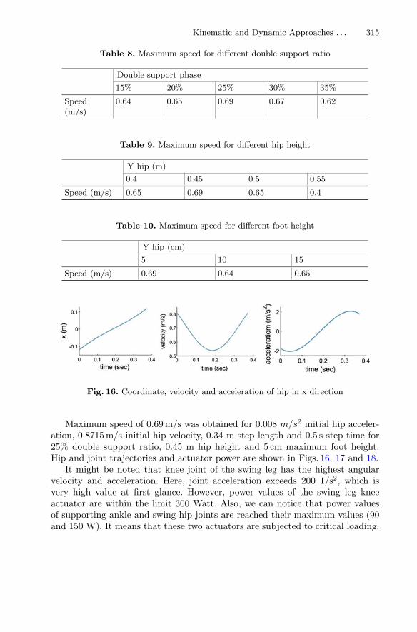
Fig. 16. Coordinate, velocity and acceleration of hip in x direction

Maximum speed of 0.69 m/s was obtained for 0.008 m/s2 initial hip acceler-ation, 0.8715 m/s initial hip velocity, 0.34 m step length and 0.5 s step time for25% double support ratio, 0.45 m hip height and 5 cm maximum foot height.Hip and joint trajectories and actuator power are shown in Figs. 16, 17 and 18.

It might be noted that knee joint of the swing leg has the highest angularvelocity and acceleration. Here, joint acceleration exceeds 200 1/s2, which isvery high value at first glance. However, power values of the swing leg kneeactuator are within the limit 300 Watt. Also, we can notice that power valuesof supporting ankle and swing hip joints are reached their maximum values (90and 150 W). It means that these two actuators are subjected to critical loading.


Fig. 17. Angles, angular velocity and angular acceleration of robot joints

Fig. 18. Motor power in robot actuators

5 Conclusions

In the paper we considered a problem of optimization gait pattern for a bipedalrobot, which maximizes its locomotion speed under joint angular velocity, accel-eration and actuator power limits. We compared two approaches for defining theoptimal leg trajectory of biped locomotion. The first one, kinematic approach,uses joint kinematic limits and utilizes dynamic programming and trapezoidalvelocity profile methods to find trajectories where joints are rotated with possi-bly the maximum allowed speed or acceleration. However, the ZMP analysis ofsuch trajectories shows that this kind of motion is unstable if there is no addi-tional compensation of the ZMP deviation from the stable one, correspondingto the center of the supporting foot. Therefore, such optimal trajectories are


applicable only if we use the upper body motion to balance the robot dynamicsduring walking.

The second approach considers the robot dynamics and solves optimiza-tion problem to find maximum speed under actuator power and stability con-straints. In contrast to kinematic approach, it allows us to use different veloc-ity/acceleration limits depending on the payload applied to the actuated joint.This allowed us to reach physical limits for the swing leg. Simulation resultsshow that robot can achieve speed up to 0.69 m/s.

Future research will be done in several directions. Firstly, the developed app-roach will be applied to frontal plane motion. Secondly, we will utilize verticalhip motion to increase our performance. And finally optimization problem willbe solved not only for straight motion, but also for walking along arbitrary tra-jectories.

Acknowledgements. This research has been supported by Russian Ministry of Edu-cation and Science as a part of Scientific and Technological Research and Devel-opment Program of Russian Federation for 2014–2020 years (research grant IDRFMEFI60914X0004) and by Android Technics company, the industrial partner ofthe research.

References

1. Wright, J., Jordanov, I.: Intelligent approaches in locomotion - a review. J. Intell.Robot. Syst. 80, 255–277 (2014)

2. Sakagami, Y., Watanabe, R., Aoyama, C., Matsunaga, S., Higaki, N., Fujimura, K.:The intelligent ASIMO: System Overview and Integration, pp. 2478–2483. IEEE,New York (2008)

3. Ogura, Y., Aikawa, H., Shimomura, K., Kondo, H., Morishima, A., Lim, H.-o.,Takanishi, A.: Development of a New Humanoid Robot WABIAN-2. pp. 76-81.IEEE, New York (2006)

4. Shamsuddin, S., Ismail, L.I., Yussof, H., Zahari, N.I., Bahari, S., Hashim, H., Jaffar,A.: Humanoid Robot NAO: Review of Control and Motion Exploration. pp. 511–516. IEEE, New York (2011)

5. Feng, S., Whitman, E., Xinjilefu, X., Atkeson, C.G.: Optimization-based full bodycontrol for the DARPA robotics challenge. J. Field Robot. 32, 293–312 (2015)

6. Vukobratovic, M., Borovac, B.: Zero-moment point - thirty five years of its life.Int. J. Hum. Robot. 01, 157–173 (2004)

7. Shafii, N., Abdolmaleki, A., Lau, N., Reis, L.P.: Development of an OmnidirectionalWalk Engine for Soccer Humanoid Robots (2015)

8. Albert, A., Gerth, W.: Analytic path planning algorithms for bipedal robots with-out a trunk. J. Intell. Robot. Syst. 36, 109–127 (2003)

9. Sato, T., Sakaino, S., Ohnishi, K.: Real-time walking trajectory generation methodwith three-mass models at constant body height for three-dimensional bipedrobots. IEEE Trans. Indust. Electron. 58, 376–383 (2011)

10. Ha, T., Choi, C.-H.: An effective trajectory generation method for bipedal walking.Robot. Autonom. Syst. 55, 795–810 (2007)

11. Erik Cuevas, D.Z.: Polynomial Trajectory Algorithm for a Biped Robot (2010)


12. Katoh, R., Mori, M.: Control method of biped locomotion giving asymptotic sta-bility of trajectory. Automatica 20, 405–414 (1984)

13. Furusho, J., Masubuchi, M.: Control of a dynamical biped locomotion system forsteady walking. J. Dyn. Syst. Meas. Control 108, 111–118 (1986)

14. Liu, C., Wang, D., Chen, Q.: Central pattern generator inspired control for adaptivewalking of biped robots. IEEE Trans. Syst. Man Cybern. Syst. 43, 1206–1215(2013)

15. Kajita, S., Kanehiro, F., Kaneko, K., Fujiwara, K., Harada, K., Yokoi, K.,Hirukawa, H.: Biped walking pattern generation by using preview control of zero-moment point. In: Proceedings of the IEEE International Conference on Roboticsand Automation, 2003. ICRA ’03, vol. 1622, pp. 1620–1626 (2003)

16. Katayama, T., Ohki, T., Inoue, T., Kato, T.: Design of an optimal controller for adiscrete-time system subject to previewable demand. Int. J. Control 41, 677–699(1985)

17. Goswami, A.: Postural stability of biped robots and the foot-rotation indicator(FRI) point. Int. J. Robot. Res. 18, 523–533 (1999)

18. Dau, V.-H., Chew, C.-M., Poo, A.-N.: Achieving energy-efficient bipedal walkingtrajectory through GA-based optimization of key parameters. Int. J. Hum. Robot.6, 609–629 (2009)

19. Liu, Z., Wang, L., Chen, C.L.P., Zeng, X., Zhang, Y., Wang, Y.: Energy-efficiency-based gait control system architecture and algorithm for biped robots. IEEE Trans.Syst. Man. Cybern. Part C (Appl. Rev.) 42, 926–933 (2012)

20. Khusainov, R., Klimchik, A., Magid, E.: Swing leg trajectory optimization for ahumanoid robot locomotion. In: 2016 13th International Conference on Informaticsin Control, Automation and Robotics (ICINCO) (2016)

21. Khusainov, R., Shimchik, I., Afanasyev, I., Magid, E.: Toward a human-like loco-motion: modelling dynamically stable locomotion of an anthropomorphic robot insimulink environment. In: 2015 12th International Conference on Informatics inControl, Automation and Robotics (ICINCO), pp. 141–148 (2015)

22. Nakamura, M.: Trajectory planning for a leg swing during human walking. IEEEInt. Conf. Syst. Man Cybern. 1, 784–790 (2004)

23. Khusainov, R., Sagitov, A., Afanasyev, I., Magid, E.: Bipedal robot locomotionmodelling with virtual height inverted pendulum in Matlab-Simulink and ROS-Gazebo environments. J. Robot. Netw. Artif. Life 3 (2016)

24. Tangpattanakul, P., Artrit, P.: Minimum-time trajectory of robot manipulatorusing Harmony Search algorithm. In: 6th International Conference on ElectricalEngineering/Electronics, Computer, Telecommunications and Information Tech-nology, 2009. ECTI-CON 2009, pp. 354–357 (2009)

25. Si, J., Yang, L., Chao, L., Jian, S., Shengwei, M.: Approximate dynamic program-ming for continuous state and control problems. In: 17th Mediterranean Conferenceon Control and Automation, 2009. MED ’09, pp. 1415–1420 (2012)

26. Khusainov, R., Afanasyev, I., Magid, E.: Anthropomorphic robot modelling withvirtual height inverted pendulum approach in Simulink: step length and periodinfluence on walking stability. In: The 2016 International Conference on ArtificialLife and Robotics (ICAROB 2016), Japan (2016)

27. Klimchik, A., Pashkevich, A., Caro, S., Chablat, D.: Stiffness matrix of manipula-tors with passive joints: computational aspects. IEEE Trans. Robot. 28, 955–958(2012)

28. Klimchik, A., Chablat, D., Pashkevich, A.: Stiffness modeling for perfect and non-perfect parallel manipulators under internal and external loadings. Mech. Mach.Theory 79, 1–28 (2014)


29. Klimchik, A., Pashkevich, A., Chablat, D., Hovland, G.: Compliance error compen-sation technique for parallel robots composed of non-perfect serial chains. Robot.Comput. Integr. Manufact. 29, 385–393 (2013)

30. Klimchik, A., Bondarenko, D., Pashkevich, A., Briot, S., Furet, B.: ComplianceError Compensation in Robotic-Based Milling. In: Ferrier, J.-L., Bernard, A.,Gusikhin, O., Madani, K. (eds.) Informatics in Control, Automation and Robotics:9th International Conference, ICINCO 2012 Rome, Italy, July 28–31, 2012 RevisedSelected Papers, pp. 197–216. Springer International Publishing, Cham (2014)

31. Klimchik, A., Furet, B., Caro, S., Pashkevich, A.: Identification of the manipulatorstiffness model parameters in industrial environment. Mech. Mach. Theory 90,1–22 (2015)

32. Majima, K., Miyazaki, T., Ohishi, K.: Dynamic gait control of biped robot basedon kinematics and motion description in Cartesian space. Electr. Eng. Jpn. 129,96–104 (1999)

33. Mitobe, K., Capi, G., Nasu, Y.: Control of walking robots based on manipulationof the zero moment point. Robotica 18, 651–657 (2000)

34. Ude, A., Atkeson, C.G., Riley, M.: Programming full-body movements forhumanoid robots by observation. Robot. Autonom. Syst. 47, 93–108 (2004)

35. Yamaguchi, J., Soga, E., Inoue, S., Takanishi, A.: Development of a bipedalhumanoid robot-control method of whole body cooperative dynamic biped walk-ing. In: 1999 IEEE International Conference on Robotics and Automation, 1999.Proceedings, vol. 361, pp. 368–374 (1999)

kinematic and dynamic approaches in gait optimization for

Documents