kick detection using downhole weight measurements
TRANSCRIPT

Kick detection using downhole weightmeasurements
Alberto Joseph Cheru
Petroleum Engineering
Supervisor: Sigve Hovda, IGP
Department of Geoscience and Petroleum
Submission date: August 2017
Norwegian University of Science and Technology


i
Acknowledgement Foremost, we would like to express my profound gratitude to my supervisor, Associate Professor
Sigve Hovda for his tireless supervision, guidance, valuable suggestions and remarkable interest
which paved a way to the accomplishment of this thesis.
My sincere thanks are due to EnPe-NORAD, and Statoil under Angolan Norwegian Tanzanian
Higher Education Initiative (ANTHEI) project for financial support throughout my studies. Also I
highly appreciate the support from the University of Dar es Salaam (UDSM), at the Department
of Chemical and Mining Engineering (CME) for hosting and allowing me to use their facilities
during my thesis work.
Last but not least, I would like to express my heartfelt and special appreciations to my family
members for their prayers, moral support and guidance they provide to me in my life and
throughout my studies. My parents, Mr and Mrs Joseph Cheru are real the best mentors I can ever
have in my life.

ii
Abstract Drilling optimization is a key tool for a company which wants to achieve the best drilling
performance and ultimately low effective drilling cost. In achieving these, use of correct weight
on bit(WOB) as part of drilling optimization is inevitable in order to achieve an optimal rate of
penetration. Not only that weight on bit is important in optimizing drilling performance, but also
can be used to quickly anticipate the downhole conditions using downhole weight on bit
measurements.
This thesis presents kick detection models based on different drilling parameters which are directly
related to weight measurements especially downhole weight on bit. The drilling parameters which
were highly considered in modelling are mud weight and buoyancy factor. In the analysis on how
these parameters may change during drilling operation, the mathematical models were subjected
to different factors including gas fraction, bottomhole pressure, temperature and cuttings
concentration in the well. All these factors were found to affect mud weight and buoyancy factor
and gas fraction was found to have high impact on mud weight and buoyancy factor. Well
geometry and drill string geometry were also taken into account in developing mathematical
models which take into account geometry of the drill string. Two models were developed including
the Law of Archimedes model and the Force – Area model. The two models were used to calculate
the hookload at the surface and it was determined that both give approximately the same results of
surface hookload with the Archimedes model being more accurate.
Finally, mathematical models for mud weight and buoyancy factor which use downhole weight on
bit were developed. It was revealed that the analytical torque and drag model can simply be used
to calculate downhole weight on bit from surface weight measurements. Dependence of weight on
bit on wellbore friction was taken into account. The torque and drag model was used to calculate
downhole weight on bit using real time drilling data from well 47 – 8 – 5. Computer program was
created to iteratively simulate hookload values to match the measured hookload. The simulation
was found to give hookload values close to measured values which were then converted into bulk
density and buoyancy factor. Bulk density and buoyancy factor calculated from surface hookload
values were found to be sensitive to change in downhole weight on bit and drill string weight thus
indicating that downhole weight on bit if calculated accurately can predict the onset of gas kick.

iii
Table of Contents Acknowledgement .......................................................................................................................... i!
Abstract .......................................................................................................................................... ii!
Table of Contents ......................................................................................................................... iii!
List of Figures ............................................................................................................................... vi!
List of Tables ............................................................................................................................... vii!
1.0! Introduction ....................................................................................................................... 1!
1.1! Methods Used to Detect a Kick .................................................................................... 2!
1.2! Sources of Kick in the Well .......................................................................................... 4!
1.2.1! Gas/Water Cut Mud .................................................................................................... 4!
1.2.2! Insufficient Mud weight ............................................................................................... 4!
1.2.3! Improper fill-up ........................................................................................................... 4!
1.2.4! Swab & heave effect .................................................................................................... 4!
1.2.5! Lost Circulation .......................................................................................................... 4!
1.2.6! Gas diffusion ............................................................................................................... 5!
2.0! Modelling of a Gas Kick ................................................................................................... 6!
2.1! Current Methods used in Calculation of Buoyancy Factor ...................................... 6!
2.1.1! The Generalized Law of Archimedes .......................................................................... 6!
2.1.2! The Force – Area Method (Piston Method) ................................................................ 7!
2.2! Buoyancy Factor, ! ....................................................................................................... 8!
2.3! Derivation of Buoyancy Factor .................................................................................... 8!
2.4! Factors Affecting Buoyancy Factor in the Wellbore ................................................. 9!
2.4.1! Mud Weight ................................................................................................................. 9!
2.4.2! Gas Fraction ............................................................................................................. 10!
2.4.3! Cuttings in the Mud ................................................................................................... 11!
2.4.4! Drill String Rotation ................................................................................................. 11!
2.5! Density of a Mud – gas mixture as a Function of Gas Fraction ............................. 12!
3.0! Gas fraction and Mud Weight as a Function of Time ................................................. 14!
3.1! Modelling Gas fraction ............................................................................................... 14!

iv
3.2! Modelling Mud Weight as a Function of Time ........................................................ 18!
4.0! Mud Weight as a Function of Pressure and Temperature .......................................... 20!
5.0! Mud Weight as a function of Cuttings Concentration ................................................ 23!
5.1! Modelling Mud Weight as a Function of Cuttings ................................................... 23!
5.2! Modelling Hydrostatic Pressure as a Function of Cuttings .................................... 23!
6.0! Modelling of Buoyancy Factor ....................................................................................... 26!
6.1! Buoyancy Factor as a Function of Gas Fraction ...................................................... 26!
6.2! Buoyancy Factor as a Function of Temperature and Pressure .............................. 27!
6.3! Buoyancy Factor as a Function of Time ................................................................... 28!
6.4! Buoyancy Factor as a Function of Cuttings Concentration .................................... 30!
7.0! Bottomhole Pressure and Gas Fraction ........................................................................ 33!
7.1! Variation in Bottomhole Pressure due to Gas Fraction .......................................... 33!
7.2! Simulation of Bottomhole Pressure ........................................................................... 34!
7.2.1! Algorithmic Steps in simulating for bottomhole Pressure, !" ................................. 35!
8.0! Modelling Buoyancy Factor for Vertical Well ............................................................. 37!
8.1! Buoyancy Factor of a Composite Drill String in a Vertical Well ........................... 38!
8.1.1! Buoyancy Model by Piston Method .......................................................................... 39!
8.1.2! Buoyancy Model by Law of Archimedes ................................................................... 40!
8.1.3! The Piston Buoyancy Model vs. Archimedes Buoyancy Model. ............................... 42!
9.0! Modelling Buoyancy Factor for a Deviated Well ......................................................... 45!
9.1! ∆TVD for Curved Section by Minimum Curvature Method .................................. 49!
9.2! Wellbore Profile for Well AA .................................................................................... 50!
9.3! Buoyancy Model for Deviated Wellbore ................................................................... 52!
10.0! Weight on Bit(WOB) as a Kick Indicator .................................................................... 55!
10.1! DWOB vs. SWOB ....................................................................................................... 55!
10.2! Estimation of DWOB from SWOB ........................................................................... 57!
10.2.1! Converting SWOB into DWOB ............................................................................. 58!
10.2.2! Steps in Calculating DWOB from SWOB ............................................................. 59!
10.3! Mud Weight and Buoyancy Factor from DWOB .................................................... 61!

v
11.0! Conclusion and Recommendations ............................................................................... 63!
11.1! Conclusion ................................................................................................................... 63!
11.2! Recommendations ....................................................................................................... 64!
References .................................................................................................................................... 65!

vi
List of Figures Figure 2-1: Forces acting on the submerged body ..................................................................... 7!
Figure 2-2: Drill pipe submerged in a vertical well(Aadnoy & Kaarstad, 2006) ...................... 8!
Figure 3-1: Gas rising up the annulus ...................................................................................... 15!
Figure 3-2: Determination of gas height in the annulus .......................................................... 16!
Figure 3-3: Gas expanding in the well ..................................................................................... 17!
Figure 3-4: Mud weight as a function of time ......................................................................... 18!
Figure 5-1: Relative Hydrostatic pressure under influence of cuttings ................................... 24!
Figure 5-2: Relative Hydrostatic pressure under influence of cuttings ................................... 25!
Figure 6-1: Relationship between buoyancy factor and gas fraction ....................................... 27!
Figure 6-2: Buoyancy factor as a function of depth and time .................................................. 29!
Figure 6-3: Effects of cuttings on buoyancy factor ................................................................. 31!
Figure 6-4: Effect of density differences on buoyancy factor ................................................. 31!
Figure 6-5: Influence of density differences on buoyancy factor ............................................ 32!
Figure 7-1: Pressure exerted by a small lamina ....................................................................... 33!
Figure 7-2: Apparent mud weight as a function of degree of gas fraction .............................. 35!
Figure 7-3: Mud weight as a function of depth and time ......................................................... 36!
Figure 8-1: Vertical Wellbore Schematic ................................................................................ 37!
Figure 8-2: Composite drill string ............................................................................................ 39!
Figure 8-3: Free body diagram for the drill collar ................................................................... 40!
Figure 8-4: Different densities and different pipe sizes scenario ............................................ 41!
Figure 8-5: Archimedes and Piston models compared ............................................................ 44!
Figure 9-1: Schematic view of a deviated borehole ................................................................. 45!
Figure 9-2: Weight of the drill pipe in a deviated borehole ..................................................... 46!

vii
Figure 9-3: Forces acting on a drill pipe submerged in the drilling fluid ................................ 47!
Figure 9-4: Buoyant force due to pressure differences ............................................................ 48!
Figure 9-5: Projection of a wellbore in a vertical plane ........................................................... 49!
Figure 9-6: Wellbore profiles ................................................................................................... 52!
Figure 9-7: Buoyancy factor in a deviated well ....................................................................... 54!
Figure 10-1: DWOB/SWOB vs. Bit depth .............................................................................. 57!
Figure 10-2: Measured and calculated downhole weight on bit .............................................. 60!
Figure 10-3: Hookload, density and buoyancy factor calculated from DWOB ...................... 61!
List of Tables Table 8-1: Data for tapered drill string(Aadnoy & Kaarstad, 2006) ........................................ 43!
Table 8-2: Results from Archimedes and Piston Buoyancy Models ....................................... 43!
Table 9-1: Well path data for deviated well(Aadnoy & Kaarstad, 2006) ................................ 50!
Table 9-2: Results from minimum curvature model ................................................................ 51!
Table 10-1: Real - Time Drilling Data from 1567.7m to 1569.2m for Well 47-8-5 ............... 56!
Table 10-2: RTDD during tripping operation for well 47-8-5 ................................................. 59!

1
1.0! Introduction
Influx is an undesirable flow of formation fluid into the wellbore that is below the kick
tolerance(Aadnoy & Kaarstad, 2006; Gupta et al, 2013; Hollman et al, 2016). This fluid invasion
(oil, natural gas, or water) into the well from the formation happens mainly as a result of
underbalance condition which occurs when the bottomhole pressure becomes less than the
formation pore pressure.
Kick is defined as the volume of influx that exceeds kick tolerance that cannot be safely circulated
out of the well(Hollman et al, 2016). Sometimes kick, especially gas kick can enter into the
wellbore due temporary reduction in hydrostatic pressure caused by swabbing or by drilling into
the formation that contains gas even with a suitable overbalance(Gupta et al, 2013; Jonathan Felipe
Galdino et al, 2013) and very rarely, by drilling into neighbouring producing wells(Skalle, 2015b).
It is important that kick is detected as early as possible to avoid getting into an uncontrollable
amount of influx which ultimately results into hazardous blowouts and/or loss of life and
equipments. For this reason, early kick detection, without which, kicks would become more
difficult to handle is of paramount importance.
Detecting kicks earlier helps to take necessary measures in controlling them with the proper kick
handling techniques without causing any hazardous event such as formation damage(Velmurugan
et al, 2015). In a normal situation, a gas kick is removed by circulating the well using surface
adjustable choke(Rader et al, 1975).
According to Swanson et al (1997), early kick detection is of crucial importance in slimhole
wellbores and small annular volumes are required to maintain integrity of the well, which means
that allowable kick volumes must be small.
A number of kick detection techniques have been developed and implemented. However, the
increase in complexity of well drilling operations poses the need for early, more accurate and more
reliable kick detection methods because more deep water drilling operations with increasing tight
pressure margins have significantly increased,Velmurugan et al (2015). Stokka et al (1993)
developed a gas kick warner whose working principle is to measure the propagation time of a

2
pressure pulse travelling through the well. This method enables detection of small amounts of free
gas in the annulus while downhole.
1.1! Methods Used to Detect a Kick
It is crucial and beneficial to detect a kick at the very beginning and as quickly as possible. Early
kick detection can minimize the kick size and reduce the risk of blowout when controlling the well.
Due to technology advancement, kick-detection equipments are installed during drilling operations
which work on basis of kick indicators. There are a lot of kick indicators but the following are the
most important kick indications(Ling et al, 2015):
1. Pit gains due to the increase in the mud return flow rate
Mud is circulated outside the well to the surface and is taken to the mud pit via the mud return line.
Observing level of the mud in the pit may help to notice the change in mud volume especially
increase in mud flow. This increase in mud flow is called pit gain and is the difference between
mud inflow volume and the mud outflow volume given as Pit'()* = V)* − V-./. This method has
its drawback because the reliability of pit gain depends on size of the mud pit and the larger the
mud pit the slower the gain in the pit volume is and the less accurate this method becomes.
2. Mud flows when pumps are off
The common practice to confirm that there is occurrence of kick in the well is to switch of the
pumps and look at the flow. Mud flowing while the pumps are off sends a message that there is an
extra energy pushing the mud out of the well. This might be the fluid flowing into the well due to
formation pressure being high than the bottomhole pressure. This method may be reliable but it
seems less quick as it may be the last indicator before deciding whether it is the real or fake kick.
3. An increase in the mud return flow rate
Increase in mud flow rate can be used as a simple method to anticipate the onset of influx in the
well. When increase in mud return flow rate is observed at the surface, the main reason is influx
at the bottom caused by high pressure fluid, normally a gas. This influx sets an additional flow on
the mud displacing the denser mud as the gas keeps flowing into the well. However, sometimes
this may not be the case as well breathing(ballooning) may also be the reason for increase in mud
flow rate. Ballooning is the situation where the well releases back the mud that was taken by the

3
formation and may sometimes be confused with the kick. This drawback makes this method less
reliable as it can sometimes give a false information.
4. Gas cutting or salinity changes in the drilling fluid
Gas cutting is the crucial method to use in detecting the onset of a kick. It is the measure of how
much has is present in the mud to the total volume of the mud. This parameter affects many factors
like mud weight, surface weight and buoyancy factor all of which have interrelated to each other.
Gas cutting is sometimes known as gas fraction and its works fine depending on the type of mud
used. In the oil based mud this method may be less quick, because more gas is likely to be absorbed
than in the water based mud. If a water based mud is used and with the system to monitor change
in gas fraction in the well, then looking at other parameters associated with gas fraction may be a
quicker way to anticipate the occurrence of the kick.
5. An increase in drill string weight
Change in drill string weight is normally associated with the condition down the hole. If mud
weight is decreasing, the main reason might be increase in mud weight leading to a corresponding
decrease in buoyancy factor which ultimately affects the weight of the drill string at the surface.
On the other, increase in weight of the string may be the result of increase in buoyance factor
which is caused by mud weight being lowered from its original value. This is because there is a
direct relationship between density of the mud and buoyancy factor and this relationship will be
discussed in detail in the next chapters.
6. An abrupt increase in rate of penetration (ROP)
This method can be used to indicate the occurrence of a kick by paying attention to the change in
rate of penetration. Rate of penetration is the increase in bit depth per hour an is measured in meters
drilled per unit hour. Change in rate of penetration indicates in increase in differential pressure
which is the difference between the pore pressure and hydrostatic pressure due to mud column in
the annulus expressed as difference in equivalent densities (i.e. ρpore – 1mud). Assuming other
factors remain constant and the mud weight is unchanged, then increase in rate of penetration
indicates increase in pore pressure. The same conclusion can be drawn that if the pore pressure

4
remains constant, an increase in penetration rate indicates the decrease in mud weight which might
be caused by the mud being cut due to an influx of a low density fluid, normally a gas influx
(Skalle, 2015b).
1.2! Sources of Kick in the Well
A kick can occur when mainly when borehole pressure (BHP) drops to below the formation pore
pressure. This may happen due to the following reasons:
1.2.1! Gas/Water Cut Mud
If gas or salt water contaminates the drilling mud, the average density of the drilling fluid is
lowered. This mud weight reduction may sufficiently lower the hydrostatic bottomhole pressure
because it depends on density of the mud. Gas contamination has big impact on lowering mud
weight than water(Rommetveit et al, 2003)
1.2.2! Insufficient Mud weight
Insufficient mud weight means mud weight which cannot provide a sufficient pressure over the
formation pore pressure at the bottom of the well at a given depth. This leads to underbalanced
condition at the bottom of the well which may result into influx of the low density fluid.
1.2.3! Improper fill-up
This may happen when the drill pipe (DP) is pulled out of the hole (POOH) and the hole is not refilled with a sufficient mud to take the space of the drill string pulled out of the hole. If the fluid cannot fill the volume of the drill string, the level of the mud in the annulus which may fail to maintain the bottomhole pressure over formation pore pressure.
1.2.4! Swab & heave effect
Swabbing may create swab pressure leading into an abrupt lowering of bottomhole pressure to below the formation pore pressure if a certain volume of mass/steel is removed from the hole too fast. This may be due to tripping out too fast or caused by the effect of heave when the drill string is in slips on a floating drilling unit. The reduced pressure created may be sufficient to allow fluids to enter the wellbore.
1.2.5! Lost Circulation
Due to presence of fractures in the fresh formation and under overbalanced condition, drilling mud
may be lost into the formation through the fractures or thief zones. If this is more severe, reduction

5
in mud-column sufficiently to drop the mud hydrostatic pressure below the pore pressure may
occur thereby initiating a kick(Aadnøy, 2006).
1.2.6! Gas diffusion
When drilling using Oil Based Mud (OBM) in deep and high pressures and temperatures wells,
gas un expectedly diffuse and get dissolved completely in the base oil of the mud. This may occur
even when drilling in an overbalanced condition. The gas stays dissolved and it is circulated
upwards with the mud and when it reaches the pressure and/or temperature conditions favorable
for its expansion, a quick and sudden out flow of mud mixed with gas erupts at the surface
especially for high pressure and high temperature wells (Rommetveit et al, 2003)

6
2.0! Modelling of a Gas Kick
Modelling of gas kick aims at developing mathematical models that can be used to predict the
onset of a kick in the wellbore. The models that take in every possible parameter which is likely
to be affected by influx is developed. The models are developed based on whether the well is
vertical or deviated. In discussing the mathematical models, different parameters are considered
including gas fraction, cuttings concentration, temperature, pipe rotation, pressure and more
importantly buoyancy factor.
2.1! Current Methods used in Calculation of Buoyancy Factor
In calculation of buoyancy or buoyancy factor, two approaches are normally used in calculating
weight of the drill string in the wellbore. The two approaches include the Archimedes law and
piston force approach. The Archimedes law states in simplicity that the buoyancy equals the weight
of the displaced fluid. The piston method on the other hand is the uniaxial force balance applied
to each geometrical change in the string(Aadnoy & Kaarstad, 2006; Aadnoy et al, 1999).
According to Aadnoy et al (1999), if both of these methods are used correctly, they provide
identical results and on top of that, Aadnoy et al (1999) keeps arguing that the Archimedes
principle can be used for all cases.
2.1.1! The Generalized Law of Archimedes
According to Archimedes principle, buoyancy of the body is equal to the weight of the displaced
fluid in which it floats. On the other hand, this implies that buoyancy is the force acting opposite
to the gravitational weight of the body which acts downwards. It is therefore concluded in the work
by Aadnoy & Kaarstad (2006), that only pressure contributes to buoyancy and this pressure acts
on the projected vertical area. It is important to first understand the direction of gravitation so that
the projected area can be easily determined. For instance, if the gravitation acts in the z direction,
then buoyancy acts in the orthogonal plane x, y. The buoyancy force F(z) can then be determined
using:
F(z) = 7P(z)A(z)
(2.1)

7
Where P z is the hydrostatic pressure at the given depth and A z is area upon which the pressure acts and is given
by A z =7 ∫:∫;dx dy. Equation(2.1) is the general equation for buoyant force and can be applied to any geometry
of the body. For instance, if this equation is applied to an arbitrary body, say a vertical cylindrical prism shown in
Figure 2-1 of height h, the buoyant force F?, is equal to the difference between bottom and top forces acting on the
prism given as F?= F?-//-@ − 7F/-A. This force is also equal to the hydrostatic pressure given by P z = ρgz,7times
the projected area (Aadnoy & Kaarstad, 2006).
Figure 2-1: Forces acting on the submerged body
2.1.2! The Force – Area Method (Piston Method)
The piston method is based on force balance by considering forces acting throughout the drill
string. For drill string components (pipes etc.) with different outer diameters connected to form
the drill string, an area is exposed wherever there is change in size of the drill string components.
The forces acting on the drill string at these exposed areas are equal to the hydrostatic pressure
times the exposed area at the particular point of interest. Carefully and proper application of this
method gives the same weight of the drill string at the surface in spite of the fact that the forces at
the depths may be slightly different(Aadnoy & Kaarstad, 2006; Aadnoy et al, 1999).

8
2.2! Buoyancy Factor, !
Buoyancy factor is the mathematical expression which defines the effect of the fluid on the
submerged body. This effect is called buoyancy and refers to the effect by which the body
submerged in the fluid experiences a weight reduction due to an upward force (up thrust) acting,
The buoyancy effect which is expressed in terms of buoyancy factor, ! depends on density of the
fluid in the wellbore, "mud and the density of the material,7"D/EEF
, Glomstad (2012).
2.3! Derivation of Buoyancy Factor
The idea behind buoyancy factor is based on the fact that when the body is submerged into the
fluid it will measure less than its actual weight following to the famous law of Archimedes. This
weight is called the apparent weight of the body and the ratio between the decrease in weight to
the actual weight of the body is known as buoyancy factor. This can be mathematically expressed
as difference between actual weight Wa, of the body and its apparent weight Wap, divided by its
actual weight.
Figure 2-2: Drill pipe submerged in a vertical well(Aadnoy & Kaarstad, 2006)
Figure 2-2 illustrates the drill pipe submerged in a vertical well. The weight in air W(, of the drill
pipe is given by the product of its density ρD/EEF, the volume of the pipe VA)AE = AL, and the
gravitational constant g, as W()H = ρD/EEF .A.L.g where A and L are the cross sectional area and
length of the pipe respectively.

9
Suspending the drill pipe into the borehole filled with a fluid with a density ρ@.I provides a lift due to hydrostatic force acting at the bottom end of the pipe(Aadnoy & Kaarstad, 2006). This force is equal to the bottomhole pressure multiplied with the cross sectional area A, as FJ;I = ρ@.I. g. TVD. A. The net weight is given by the difference between the pipe weight in air and the buoyant force due to hydrostatic pressure. This net weight which is also known as the buoyed weight of the pipe and is given by:
W?.-;EI = W()H −7FJ;I = (ρD/EEF − ρ@.I)gAL (2.2)
Where for the case of vertical borehole, L is the same as the true vertical depth, TVD. This buoyed
weight W?.-;EI, is defined as the product of the buoyancy factor !, and the pipe weight in air as
!.W()H = W?.-;EI, which upon substitution of the definitions of W?.-;EI and W(7gives:
!.ρD/EEF .A.L.g = (ρD/EEF − ρ@.I)gAL
(2.3)
Rearrangement and simplification gives the final equation for buoyancy factor as given in (2.4).
This equation if used to estimate the weight at the of the drill string gives a correct estimate(Hovda,
2017).
! = 1 − KLMN
KOPQQR
(2.4)
Equation (2.4) gives the buoyancy factor on a body submerged in the fluid. Considering the drill
string with fluids inside and outside of the drill pipe(s), this equation becomes the simplest form
of the buoyancy factor model. The simplifying assumptions include similar inside and outside
diameters through the drill string and the same densities inside and outside the drill string.
2.4! Factors Affecting Buoyancy Factor in the Wellbore
In discussing the mathematical models, different parameters are considered including mud weight,
gas fraction, cuttings concentration, pipe rotation, side forces and well geometry
2.4.1! Mud Weight
Weight reduction due to buoyancy is mainly influenced by mud weight. The uplifting force due to
buoyancy changes with the change in density of the mud and a denser fluid reduces the effective

10
weight of the drill string pipes. A lighter mud on the other hand increases the buoyancy factor
hence reducing the uplifting effect of the drilling fluid consequently leaving the weight almost
unaffected. This direct relationship between mud weight and buoyancy factor can be deduced from
the hydrostatic pressure, PJ;I at a depth h in the well as given in equation as:
PJ;I = g h7ρ@.I
(2.5)
Equation(2.5) suggests that the lower the mud weight, the lower the hydrostatic pressure at a given
depth. Combining equation(2.4) and equation(2.5), the relationship between buoyancy factor and
hydrostatic pressure can be obtained.
! = 1 − STUN
'7J7KOPQQR
(2.6)
Many factors can lead to increase or decrease of the mud weight, so does to buoyancy factor. These
include gas entering the mud, cuttings in the mud, pressure and temperature, Kristensen (2013).
The effective mud weight of the drilling fluid can be estimated by taking into account these factors
and is called fluid mixture density or cut mud density,"@):
(Skalle, 2015a).
2.4.2! Gas Fraction
Presence of gas in the drilling fluid reduces the density of the mud. Gas is a very light fluid and
occupies large volume due to its ability to expand. When gas enters the wellbore, it mixes with the
fluid and gets dissolved into the mud depending on the mud type.
In oil based mud, a small gas kick dissolves into the mud leading to a small increase in volume as
the dissolved gas behaves as a liquid. In water based mud, the gas kick does not dissolve and hence
a small kick volume expands rapidly with time. The overall effect of the gas cut is lowering of the
mud weight and the more the gas into the mud, the lower the mud weight becomes.
The fluid mixture density, "mix of the mud depends on the amount of gas which is proportional
with gas fraction, Cgas. The gas fraction is given as a ratio of volume of the gas, Vgas to the total
volume of the fluid mixture Vmix as given in equation(2.7)

11
Cgas = VWXOVLYZ
(2.7)
2.4.3! Cuttings in the Mud
Cuttings are drilled solids present into the mud during drilling operation. The presence of cuttings
in the mud affects the effective density of the mud and normally an increase in mud weight.
Cuttings are classified by particle sizes as coarse, intermediate, mediums, ultrafine and colloidal.
Particles greater than 2000 microns are regarded as coarse cuttings, those ranging from 250 – 2000
microns are referred to as intermediate cuttings and medium cuttings range from 74 – 250 microns
(Skalle, 2015a).
Most of the drilled cuttings are heavier than density of the mud used. If taken in big fraction by
volume, the consequence is increase in density of the mud. It is by far important to have all drilled
cuttings being carried out with the mud to the surface but not exceeding the limit so as to maintain
the quality of the drilling fluid.
2.4.4! Drill String Rotation
Pipe rotation has significant effects on mud rheology as rotation affects the viscosity and density
of the mud in an indirect way. As the pipe rotates, the cuttings holding ability of the mud increases.
However, this depends on the type of mud system that is being used. According to Ozbayoglu et
al (2008), pipe rotation together with other factors have big influence on hole cleaning
performance. Rotation of the pipe increases the amount of cuttings suspended in the mud and hence
the better the cuttings removal from under the bit. If more cuttings are suspended into the mud,
density of the mud increases accordingly.
Experimental study by Ford et al (1990) , pipe rotation affects development of cuttings bed
revealed that pipe rotation have insignificant effect on minimum fluid transport velocity if low
viscosity fluid is used. In medium to high viscous fluids, pipe rotation influences the minimum
fluid transport velocity.
Increasing pipe rotation decreases the minimum velocity required to suspend cuttings into the mud.
In the experimental study conducted by Sifferman & Becker (1992), pipe rotation was one of the
factors which highly affect cuttings suspension in the mud and that the higher the speed of pipe
rotation, the more cuttings are eroded from the cuttings bed.

12
It was demonstrated using Taylor vortices in Lockett et al (1993) and pointed out that pipe rotation
is crucial in removing cuttings and suspending them into the mud. McCann et al (1995) in his study
on pressure loss in narrow annuli concluded that increase in pipe rotation increases pressure loss
especially in a turbulent fluid flow regime and vice versa is for lamina flow regime. Also a similar
conclusion was drawn by on pipe rotation that there exists a positive relationship between pipe
rotation and pressure drop such that the higher the speed of pipe rotation the higher the pressure
drop. Saasen (1998) observed that pipe rotation aids to transport large volumes of cuttings when
polymerized water based mud is used.
All these observations infer that pipe rotation indirectly affects the density of the mud in the same
manner as it does to cuttings transportation efficiency. Increasing hole cleaning efficiency suggests
that more cuttings are carried with the mud. This concludes that mud weight will increase because
more cuttings are present into the mud. On the other hand, increase in pressure loss due to pipe
rotation as previously discussed signifies reduction in mud weight. This indirect effect of pipe
rotation might be due to lowering of mud viscosity which significantly reduces the ability of the
mud to hold more cuttings.
Therefore, pipe rotation affects mud weight in both positively and negatively ways. If other factors
are kept constant, then mud weight increases with increase in pipe rotation. On the other hand,
mud weight decreases with pipe rotation if effect of cuttings concentration and other factors are
kept constant.
2.5! Density of a Mud – gas mixture as a Function of Gas Fraction
Change in volume of the gas phase in the mud – gas mixture with changing temperature and
pressure as gas rises up the annulus causes the density of the mixture to change. However, for
simplicity, it is reasonable to assume that the volume of the liquid phase does not change with
temperature and pressure i.e. the volume of the liquid phase is constant. In this sub - section the
mud-gas mixture is treated as a homogeneous fluid for a particular temperature and pressure
condition and therefore the density of the cut mud can be derived from the law of conservation of
volume and mass as follows. The mass and volume of the mixture, Mmix and Vmix is simply the
sum of the masses and volumes of the two phases as:

13
Mmix = Mmud + Mgas
Vmix = Vmud + Vgas
(2.8)
Substitution of the definition of mass in terms of volume and density gives:
ρ@):V@): = ρ'(DV'(D + ρ@[email protected] (2.9)
Dividing with Vmix throughout equation(2.9) gives:
ρ@): = ρ'(D 7VWXO
VLYZ + ρ@.I7
VLMN
VLYZ
(2.10)
But since Vmud = Vmix – Vgas and upon substitution into equation(2.10) gives:
ρ@): = ρ'(D 7VWXO
VLYZ + ρ@.I7
VLYZ77]77VWXO
VLYZ = ρ'(D 7
VWXO
VLYZ + ρ@.I7 17 −7
VWXO
VLYZ
(2.11)
Using the definition given in equation(2.7), the ratio of the gas volume Vgas to the total volume of
the mixture Vmix is equal to the gas fraction Cgas. Substitution of equation(2.11) into equation(2.7)
gives the final equation for density of the gas cut mud ρ@): in terms of gas fraction Cgas.
ρ@): = ρ'(DC'(D + ρ@.I7 17 −7C'(D (2.12)
Equation(2.12) gives the variation of mud weight as a function of gas fraction without taking into
account that gas fraction varies with time in the well bore. The variation of mud weight as a
function of the time due to the dynamic change of gas fraction will be established following to the
derivation of gas fraction as a function of time.

14
3.0! Gas fraction and Mud Weight as a Function of Time
Gas fraction is the amount by volume of gas present in the mud which is expressed as a percent of
gas in the total volume of the mud - gas mixture. Equation(2.7) gives the gas fraction as the ratio
of the volume of gas in the mud to the total volume of the mud – gas mixture. Gas fraction has a
big impact on the effective density of the drilling fluid due to the tendency of gas to expand as
pressure decreases. It is therefore important to note that while gas influx leads to decrease in
bottomhole pressure, it also creates its possibility to expand as it rises up in the annulus.
Normally, gas expansion occurs when gas is on its way out as the mud circulates and with time
the annulus gets filled with gas if proper control over gas expansion is not taken. In this section
mathematical model of a gas fraction is developed to understand the behavior of the gas in terms
of its fraction in the mud as a function of time the gas is allowed to expand. Assumptions put
forward in developing the model include two phase flow during circulating the gas out of the well
and that gas obeys the real gas behavior.
3.1! Modelling Gas fraction
Gas fraction is a critical parameter to take into account when evaluating the variation of buoyancy
factor in the well during a gas kick. Gas expands as it is circulated out of the wellbore. As the gas
expands, more drilling fluid overlying the gas column is displaced causing increase in flow rate in
the mud return line. If mud flow rate is used as an indicator of the influx, then the kick is indicated
by the sudden rise in the mud flow rate in the mud return line.
Expansion of gas is caused by the decrease of the hydrostatic pressure of the mud overlying the
gas column. This gas column is a function of time because, at any time t, the distance moved by
the top of the gas column can be estimated using the velocity of the gas. During circulating gas out
of the well, gas may behave as dispersed gas bubbles or gas slugs in the mud (Skalle, 2015b).The
gas velocity depends on the behavior of the gas in the mud as the gas is being circulated out.
Different literatures and experimental works have been performed and it has been observed that
the velocity of the gas phase in the mud is a function of the velocity of the fluid mixture U@): and
it was further deduced that this velocity depends on the type of the gas whether it is dispersed gas
bubbles or gas slugs(Skalle, 2015b; Skalle et al, 1991). The velocity of the mud – gas mixture,7U@):

15
is calculated from the mud and gas flow rates in the well as U@):(t)7= aLMNb7aWXO
c. Where [email protected] is
the mud flow rate, q'(D is the rate of gas influx and A is the annular capacity. The velocity of the
gas is given as:
U'(D(t) = 71.27Ughi 7+ 70.2777777777777for7dispersed7bubbles
t1.27Ughi 7+ 70.4777777777777777777777777777777for7gas7slugs7
(3.1)
The distance moved by the top of the gas is D(t) and can be estimated as a function of time t from
when the kick is taken as shown in Figure 3-1
Figure 3-1: Gas rising up the annulus
Assuming that gas behaves as dispersed bubbles, the distance D(t) can expressed as:
D t = 7Uxyzt (3.2)
The depth h(t) from surface to the top of the gas column (mud-column overlying the gas column)
can be estimated from the well depth minus the instantaneous distance covered by the gas column
as:
h t = 7H}~tt − D t (3.3)

16
Where H�ÄÅÅ is the well depth and equation(3.3) can be used to calculate the hydrostatic
pressure of the mud column overlying the gas column at any time t. This is just the mud weight
multiplied with the depth h(t) and the gravitational constant. This is given as:
P t = 7ρgÇÉ7g7hgÇÉ t (3.4)
Where ρ@.I is the mud weight at the time kick is taken and P t is the instantaneous hydrostatic
pressure of the mud column overlying the gas column.
Figure 3-2: Determination of gas height in the annulus
As shown in Figure 3-2, gas height at time t is shown as h'(D(t) and P(t) is the pressure at any time
acting on top of the gas column. Using the ideal gas equation, the comparison between P(t) and PÑ
can help to estimate the gas height, h'(D(t). Assuming annular capacity is the same throughout the
borehole, the relationship between P t and PÑ is given as PÑLÜ)áÜ7 = P t 7h'(D t . Therefore, the
height of the gas column as a function time t is given as:
h'(D(t) = 7PÑ7
P tLÜ)áÜ
(3.5)

17
Where PÑ is the hydrostatic pressure of the original mud just before gas kick was taken and is given
by PÑ = ρ@.I7Hwell g and LÜ)áÜ is the initial gas height at the time kick was taken.
Figure 3-3: Gas expanding in the well
Figure 3-3 shows how gas expansion over time by simulating for gas height using equation(3.5).
In this particular example, gas height was simulated by assuming a certain amount of gas enters
inters the well due to underbalance and instantly after being detected, it gets circulated out while
regaining control of the well. In this case, a gas influx flowing at the rate of 1.89m3/min(500gpm)
into the well flowing at the rate of 3.4m3/min (900gpm). The kick is assumed to be taken at a depth
4000m and the gas and mud are assumed to form a two phase flow.
As shown in Figure 3-3, gas expansion takes place slowly until the gas expands enough to reach
to a threshold amount. This threshold is the gas volume above which gas expands tremendously
which may lead to more mud being displaced from the well. In this particular example, the
threshold gas height was about 50m which took about 60minutes. At this height, the gas expanded
two times to about 100m and finally to about 490m before the gas head reaches to the surface.
Due to gas expansion in the well as it is circulated out, the mud and gas columns keep changing
with time. As the gas column increases due to expansion, the mud column above the gas column
decreases correspondingly. This means that gas expansion displaces more mud in the annulus as
gas is allowed to expand.
At this stage gas fraction can be deduced from the gas height given in equation(3.5) by estimating
the volume of occupied by gas at time t and the volume of the mud in the well. This volume
changes with time and is contributed by gas volume due to expansion Vexpa(t) and gas volume from

18
influx, Vinf (t). The gas volume due to expansion is obtained by multiplying gas height given in
equation(3.5) and the annular space(area) as Vexpa (t) = h'(D(t) Aan where Aan is the area of the
annulus. The gas volume due to influx, Vinf (t) is given by V)*âF(t) = qgas t where t is the time taken
after kick occurrence and this gives the gas volume at time t as:
V'(D(t) = Vexpa (t) + V)*âF(t) (3.6)
Similarly, Volume of mud in the well is [email protected](t) = [email protected](t) Aan + [email protected] where [email protected](t) is the
height occupied by the mud above the gas head as shown in Figure 3-2. The total volume in the
annulus is given by the sum of mud volume and gas volume in the annulus at t. This is given as:
V/-/(F(t) = V'(D(t) + [email protected](t) (3.7)
The gas fraction is calculated using equation(2.7) as:
C'(D(t) = VWXO(/)7VPäPXR(/)7
(3.8)
3.2! Modelling Mud Weight as a Function of Time
In section 3.1 above, gas fraction as a function of time is derived and is given by equation(3.8).
The expansion of the gas in the annulus causes the density of the mud – gas mixture becomes
dependent on time as well. Combining equation(2.12) and (3.8) gives density of the mud - gas
mixture as a function of time as:
ρ@): t = 7 ρ'(DC'(D(t) + (1−C'(D(t))7ρ@.I (3.9)
Figure 3-4: Mud weight as a function of time

19
Figure 3-4 shows how mud weight can change with time due to gas expansion in the well. The
model given in equation(3.9) helps to estimate the density of the gas – mud mixture over time
taking into account increase in volume due to expansion. This model reveals that mud weight
drops abruptly at the start when the gas influx starts and takes a gradual decrease over time. This
decrease may take a short interval of time to be noticed and normally setting upper and lower
boundaries may help to identify the abnormality in the mud.
In Figure 3-4 the lower and upper boundaries are set to easily figure out how long mud weight
drops to below the lower limit. A normal mud weight is the one in between the upper and lower
boundaries and below or above it is said to be an abnormal mud weight. In this simulation, the
mud weight dropped to below the lower limit just in about 15 minutes. This shows how rapidly
the gas kick can be in affecting density and downhole pressure if not properly controlled.

20
4.0! Mud Weight as a Function of Pressure and Temperature
The presence of gas component in the mud makes the density of the cut mud, ρ@): change with
depth and time. The depth at which the gas kick is taken determines how much it can have impact
on mud weight reduction and the longer the kick remains uncontrolled, the more the mud is cut.
However, this is an indirect impact as the mostly affected parameter due to gas kick is the
hydrostatic pressure which is a function of depth. Changing pressure and sometimes temperature
in the bore hole changes the corresponding mud weight due to expansion of gas. Therefore, it is
important to obtain the actual volume of the gas under changing conditions using the real gas law
PV = ZnRT. With the gas volume, V'(Dã at condition 1 known, the volume of the gas at condition
2 unknown, can be obtained using:
V'(Då(Tå, På) = 7V'(DãZåPãTåZãPåTã
(4.1)
Where V'(Då(Tå, På) is the volume of the gas at the new temperature and pressure conditions and
Tå and På are the temperature and pressure respectively at the new conditions. The ratio of the
volumes at the new conditions 2 to that at the previous conditions 1 gives the amount of how much
gas expands between the two states. This factor is known as gas expansion factor K, and can be
expressed as:
K =V'(DåV'(Dã
= 7ZåPãTåZãPåTã
(4.2)
Similarly, the density of the gas at anew temperature and pressure condition, ρ'(Då with the density
of gas at condition 1 known, ρ'(Dã7can be obtained using the law of conservation of mass. At the
two conditions, mass of the gas in well remains constant meaning that only volume and density of
the gas can change. Since density is inversely proportional to volume, equation(4.2) gives the
relationship between densities at the two conditions of temperature and pressure as.
ρ'(Då Tå, På = 77K]ãρ'(Dã (4.3)

21
Change in the volume of gas component due to change in temperature and pressure as given in
equation(4.2) results into the change in volume of the mud – gas mixture. The new volume of the
mud-gas mixture at new condition 2 can be expressed in terms of the new volume of the gas, Vgas2
as:
Vmix2(Tå, På) = Vmud1 + V'(Då(Tå, På) (4.4)
Where Vmix2(Tå, På) is the volume the mud – gas mixture at the new temperature and pressure
conditions and Vmud1 is the volume of liquid phase in the well. Since the volume of the liquid phase
is given by Vmud1 =7V@):ã (1− C'(Dã) where V@):ã7is the volume of the mud−gas mixture at
condition 1. Substituting equation(4.2) and the definition of Vmud1 into equation(4.4) and
rearranging gives:
V@):å(Tå, På) = 7V@):ã (1 −7C'(Dã) 7+7êëSíìë
êíSëìí
VWXOí
VLYZí (4.5)
Since VWXOíVLYZí
= C'(Dã, them substituting this definition into equation(4.5) gives:
V@):å(Tå, På) = 7V@):ã (1 −7C'(Dã) 7+ 7KC'(Dã (4.6)
Equation(4.6) can be used to estimate the new gas fraction C'(Då at the new temperature and
pressure at conditions 2 using the definition of gas fraction given in equation(2.7) but in this case
with Vgas = Vgas2(Tå, På) and Vmix = V@):å(Tå, På) as Cgas2(Tå, På) = VWXOëVLYZë
. Combining these
definitions and equation(4.6) gives:
C'(Då(Tå, På) = VWXOí
îëïíñëîíïëñí
7VLYZí7 (ã]7óWXOí)7b7îëïíñëîíïëñí
óWXOí =
îëïíñëîíïëñí
7òWXOí
7òLYZí
7 (ã]7óWXOí)7b7îëïíñëîíïëñí
óWXOí
(4.7)
Substituting VWXOíVLYZí
= C'(Dã in equation(4.7) and rearranging gives the final equation for gas fraction
C'(Då at new temperature and pressure conditions 2.
C'(Då(Tå, På) = 1 +7 ã7]7óWXOí
óWXOí
ã
ô
]ã
(4.8)
22
The mud cut density, ρ@):å(Tå, På) of the mud – gas mixture at new condition of temperature and
pressure can be deduced using equation(4.8) and the law of conservation of mass. Since mud
weight and volume do not change from one position to another, then using the law of conservation
of mass, the mass of the mixture remains constant over all temperature and pressure ranges (i.e.
M@):ã = M@):å = M@):). This allows re – definition of equation(4.6) in terms of density as õLYZ7
KLYZë ì,S = õLYZ
KLYZí (1 −7C'(Dã) 7+ 7KC'(Dã . Upon re – arrangement and simplification, the cut mud
density at the new temperature and pressure condition is given as:
ρ@):å Tå, På = 7KLYZí
ã]77óWXOí 7b7ôóWXOí7 (4.9)
Equation(4.9) shows that density of the cut mud changes with change in temperature and pressure
caused by change in gas component which changes with changing temperature and pressure. It is
indicated that the density varies directly proportional with pressure and inversely proportional with
temperature.

23
5.0! Mud Weight as a function of Cuttings Concentration
Cuttings concentration leads to an increase in mud weight due to increased solids content in the
mud. It is important to understand that drilled solids can sometimes compensate the effect of
bottomhole pressure reduction in the wellbore caused by drilled gas(Goldsmith, 1972). This
increase in bottomhole pressure is due to increase in mud weight.
5.1! Modelling Mud Weight as a Function of Cuttings
While drilling, cuttings are generated in the wellbore. The amount of cuttings depends on the rate
of penetration, and can be expressed as:
qá.//)*'D = 7ROP.π. d?)/
å
4 (5.1)
Where ROP is the rate of penetration (m/hr) and dbit is the bit diameter. The cuttings concentration
at the bottom of the wellbore also known as original cuttings concentration, Ccuttings, o is given as
the function of the pump flow rate, qpump and cuttings flow rate qcuttings, Skalle (2015a).
Cá.//)*'D,- = aüMPPY†WO
aüMPPY†WOba°ML°7≈
aüMPPY†WO
a°ML° (5.2)
Equation(5.2) gives the cuttings concentration at the bottom of the annulus. The density of the mud
mixed with cuttings at the bottom of the annulus as a function of cuttings concentration is given
as:
"@):
= "@.I
+ ("á.//)*'D
– "@.I
). Cá.//)*'D (5.3)
Equation(5.3) is valid only under assumptions that there is no gas or water influx in the well which
would affect the density of the mixture.
5.2! Modelling Hydrostatic Pressure as a Function of Cuttings
The effect of cuttings concentration on bottomhole pressure can easily be investigated by using
the relative hydrostatic pressure Prel, of the mud column with and without cuttings into the mud
assuming that the well is being drilled under the same speed such that density of the mud – cuttings
mixture, "@):
remains constant. However, if the drilling rate is not constant, the density of the mud
24
– cuttings mixture might change correspondingly. The relative hydrostatic pressure may be given
by:
Prel = "LYZ.'.ìV£
KLMN.'.ìV£ = "LYZ
KLMN=
óüMPPY†WO.KüMPPY†WO777b7(7ã7]7óüMPPY†WO7)KLMN77
"LMN
(5.4)
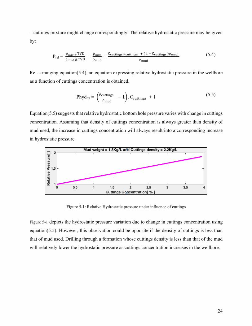
Re - arranging equation(5.4), an equation expressing relative hydrostatic pressure in the wellbore
as a function of cuttings concentration is obtained.
Phydrel = KüMPPY†WO77
"LMN
7− 1 . Cá.//)*'D + 1 (5.5)
Equation(5.5) suggests that relative hydrostatic bottom hole pressure varies with change in cuttings
concentration. Assuming that density of cuttings concentration is always greater than density of
mud used, the increase in cuttings concentration will always result into a corresponding increase
in hydrostatic pressure.
Figure 5-1: Relative Hydrostatic pressure under influence of cuttings
Figure 5-1 depicts the hydrostatic pressure variation due to change in cuttings concentration using
equation(5.5). However, this observation could be opposite if the density of cuttings is less than
that of mud used. Drilling through a formation whose cuttings density is less than that of the mud
will relatively lower the hydrostatic pressure as cuttings concentration increases in the wellbore.

25
Figure 5-2: Relative Hydrostatic pressure under influence of cuttings
Figure 5-2 shows a negative impact of solids concentration in the wellbore on hydrostatic pressure
when a formation of density less than that of drilling fluid is drilled through. This observation is
known as solid cutting where increase in cuttings concentration leads to a corresponding decrease
in the effective density of the mud – cuttings mixture. The two observations discussed can be used
as important guides to the drilling crew in notifying them when the formation changes.

26
6.0! Modelling of Buoyancy Factor
Buoyancy factor is an important parameter to use in anticipating the real condition at the bottom
of the well. It can be used to easily indicate changing conditions in the well especially change in
mud weight. This goes in line with the ability of buoyancy factor to indicate changes in pressure
which is obviously due to change in mud weight. This ability of buoyancy factor to indicate change
in mud weight and pressure in the well can be used to predict the presence of a low density
fluid(gas) in the well hence predicting the occurrence of gas kick due to its ability to change
whenever mud weight and bottomhole pressure change.
In this thesis, buoyancy factor is modelled by using parameters that can affect it directly. These
parameters include temperature, pressure, time and cuttings concentration. Buoyancy factor is
modelled as a function of each parameter to indicate how they may affect change in buoyancy
factor.
6.1! Buoyancy Factor as a Function of Gas Fraction
Buoyancy factor depends on mud weight of the drilling fluid in the wellbore. This is because
change in mud weight leads to a significant change in buoyancy factor. The decrease in mud weight
which is mainly due to influx of a formation fluid with lower density than the drilling fluid
increases the buoyancy factor. A mathematical model for buoyancy factor which takes into account
the variation of gas fraction in the mud mixture is established.
The buoyancy factor given in equation(2.4) can be expressed in terms of the gas fraction by
substituting "mud with the definition of "mix . Combining equation(2.4) and equation gives:
!@):
= 1 # óWXO7."WXO77b7 7ã7]7óWXO ."LMN7
"OPQQR
(6.1)
Rearranging equation(6.1) gives:
!@):
= 1 # 7"LMN7
"OPQQR +
óWXO7 7"LMN7]7"WXO 77
"OPQQR
(6.2)
Where C'(D7is the average gas fraction in whole well and ! = 1 # 7"LMN7
"OPQQR while
777 7"@.I
7−7"'(D
77= 7∆ρ@.I. Where ∆ρ@.I is the change in density of the mud in the well.

27
Substituting the above definitions into equation(6.2) gives the final equation for buoyancy factor, !@):
of the mud – gas mixture in terms of the buoyancy factor of the uncut mud, !.
!@):
= ! + 7∆KLMN
"OPQQR7 . C'(D
(6.3)
Where ∆ρ@.I is the density difference between that of the original mud and density of the gas
influx.
Figure 6-1: Relationship between buoyancy factor and gas fraction
Equation(6.3) suggests that buoyancy factor of the cut mud, !@):
is always greater than buoyancy
of un cut mud !. This means that buoyancy factor increases as the gas fraction, Cgas increases. If
the gas fraction is assumed to increases linearly, buoyancy factor increase linearly with gas fraction
and this can be shown in Figure 6-1 which depicts how mud weight varies with the increase in the
size of the gas influx. In this example, a mud weight equivalent to 1.5Kg/L was used as an initial
mud weight.
6.2! Buoyancy Factor as a Function of Temperature and Pressure
Changing temperature and pressure have a direct impact on buoyancy factor especially when there
is gas in the well. In section 4.0 above, effect of temperature and pressure on density of the mud
was discussed revealing that temperature and pressure influences dramatic expansion of gas taken
into the mud. Due to expansion of gas, a huge volume of mud can be displaced from the well
leading to rapid decrease in bottom hole pressure.

28
The new buoyancy factor at the new temperature and pressure can be estimated by substituting
equation(4.9) into equation(2.4) gives:
!åT, P = KLYZë ì,S
KOPQQR = 1 −
§LYZíîíïëñíîíïëñí í•7¶WXOí 7ß7îëïíñë¶WXOí7
KOPQQR
(6.4)
Rearrangement gives the new buoyancy factor as:
!åT, P = 1 − KLYZí
KOPQQR ã
ã7b7 ô7]7ã óWXOí7 (6.5)
Where K = 7êëSíìëêíSëìí
where K is the gas expansion factor. Equation(6.5) shows that gas expansion
factor increases as gas expands. Since K is always greater than 1, then the ratio ã
ã7b7 ô7]7ã óWXOí7 will
be always less than 1. This means that there is a corresponding increase in buoyancy factor as the
gas expands.
6.3! Buoyancy Factor as a Function of Time
The equation governing dependence of buoyancy factor on depth and time can be obtained by
combining equation(2.4) and (3.9) of which upon simplification gives:
!@):
(t) = !®õ
7 7+ ∆ρ@.I7C'(D(t) (6.6)
Where !®õ
= 1 − KLMN
KOPQQR is the buoyancy factor of the original mud before the gas kick is taken
and ∆ρ@.I = (ρ@.I − ρ'(D). Equation(6.6) gives the buoyancy factor at a given depth and time.
It shows that before the gas kick is taken, ρ@.I = ρ'(D and this makes ∆ρ@.I = 0, thus making
the buoyancy factor equal to that of the original mud, !®õ
as shown in Figure 6-2.

29
Figure 6-2: Buoyancy factor as a function of depth and time
Figure 6-2 shows simulation of a gas kick taken at different depths to anticipate the dependence of
buoyancy factor on depth and time. The gas kick was assumed to be taken at a rate of 1.5m™/sec
and was circulated out using a mud weighted to 1.5kg/L flowing at a rate of 7m™/sec. In this
particular example, a gas kick was assumed to be circulated out at the instant it was taken. An
assumption that gas expands as it is circulated out is also taken into account using the real gas
behavior and finally it was assumed that the gas behaves as dispersed bubbles obeying
equation(3.2).
The simulation shows that buoyancy factor is a function of both time and depth. In just 45 seconds,
buoyancy factor changed from 0.81 to 0.83 as simulated in this example assuming that a gas kick
of 1.5m3/s was taken. This increase in buoyancy factor implies that mud weight has decreased
correspondingly. Decrease in mud weight means that the ability of the mud to uplift the drill string
decreases. Depending on the intensity of the gas kick taken, decrease in mud weight depends on
time and depth as shown in Figure 6-2. However, the effect of gas expansion in the well bore on
buoyancy factor remains fairly constant for some time before an abrupt increase happens. As
shown in Figure 6-2 it took about 40 seconds before to reach to a significant increase in buoyancy

30
factor and after at about 45 seconds, buoyancy factor increased from 0.81 to about 0.83. This is
an abrupt increase of about 0.2 in just 5 seconds.
This emphasizes that depending on the size of the gas kick taken and depth at which it is taken, a
critical time and critical volume of gas have to be reached before a noticeable change in buoyancy
factor happens. This critical volume is the minimum volume due to gas expansion above which
buoyancy factor is noticeably changed due gas cutting while critical time is the minimum time
taken from when gas enters the well bore to when a significant change in buoyancy factor is
experienced.
6.4! Buoyancy Factor as a Function of Cuttings Concentration
In section 0 above, density of mud as a function of cuttings concentration was developed. In this
section, buoyancy factor as a function of cuttings concentration is established. It is important to
note that, normally density of cuttings is greater than density of the mud and cuttings grain density
from different rock types ranges from 2.2 to 2.9kg/L, Bush & Freeman (1986). Combining
equation(2.4) and equation(5.3) gives the buoyancy factor as:
!@):
= 1 # 7"LMNb7("üMPPY†WO–7"LMN).óüMPPY†WO7
"OPQQR (6.7)
Rearranging equation(6.7) gives the final equation for !@):
as follows:
!@):
= 1 # 7"LMN7
"OPQQR +
óüMPPY†WO7 7"LMN7]7"üMPPY†WO 77
"OPQQR
(6.8)
Substitution of !®õ
= 1 # 7"LMN7
"OPQQR and ∆ρ@.I = "
á.//)*'D7− 7"
@.I into equation(6.8) and rearranging
gives:
!@):
= !®õ
− 7∆KLMN77
"OPQQR7 . Cá.//)*'D
(6.9)

31
Figure 6-3: Effects of cuttings on buoyancy factor
Equation(6.9) suggests that buoyancy factor of the mixture of mud and cuttings varies linearly
with cuttings concentration and that buoyancy decreases as cuttings in the mud increases provided
that density of the mud is less than density of the cuttings. If lighter cuttings are drilled so that
density of the mud is greater than density of the cuttings, buoyancy factor will increase instead of
decreasing with cuttings concentration. The upper plot in Figure 6-3 shows the decrease in
buoyancy factor taking into account that density of the mud is less than that of the cuttings while
the lower plot shows that if density of the mud is greater than that of cuttings the buoyancy factor
increases with cuttings concentration.
Figure 6-4: Effect of density differences on buoyancy factor

32
Increase in cuttings concentration is assumed to be the same in both cases and the only difference
between the two cases is slope which determines whether the cuttings will have positive or
negative effect on buoyancy factor. In Figure 6-4 the influence of the difference between density of
the mud and that of cuttings is investigated to show how buoyancy factor varies with cuttings. In
the upper plots, density of mud less than density of cuttings was used to calculate the buoyancy
factor while in the lower plots density of mud higher than that of cuttings was used. As suggested
in equation(6.9), the rate at which the buoyancy factor increases is proportional with the difference
in the two densities or simply the slope. This effect is the same regardless of whether density of
the mud is less or greater than density of cuttings.
Differentiating equation(6.9) with respect to cuttings concentration gives the change in buoyancy
factor per unit increase in cuttings concentration as given in equation(6.10)
I!LYZ
IóüMPPY†WO777777= − 7∆KLMN7
"OPQQR7 (6.10)
Whered!@):
is the change in buoyancy factor, dCá.//)*'D is the change in cuttings concentration
and dρá.//)*'D is the change in cuttings density. Equation (6.10) suggests that change in buoyancy
factor per unit change in cuttings concentration remains constant and is proportional with the
difference between density of the mud and that of cuttings as shown in Figure 6-5. In both cases as
indicated in upper and lower plots, change in buoyancy factor is higher for higher difference in
mud weight.
Figure 6-5: Influence of density differences on buoyancy factor

33
7.0! Bottomhole Pressure and Gas Fraction
Kick models to simulate for gas kicks into the well using downhole pressure and weight
measurements need to be developed. Downhole pressure and weight gauges installed in the drill
sting can be used to obtain the dynamic pressure and weight below it for components such as
bottomhole assembly. In this thesis mathematical models for buoyancy factor are developed by
converting the pressure and weight into buoyancy factor. To simulate the reality to the fullest is
quite complicated and for that reason, in this section assumptions are included for well geometry
by trying to make the model as simple as possible.
7.1! Variation in Bottomhole Pressure due to Gas Fraction
The serious consequence of formation gas flowing into the well is on bottomhole pressure
reduction. This effect is due to the reason that gas expands rapidly and displaces large volume of
mud from the well and due to its lowest density, the overall density of the gas is cut (reduced)
which as a result decreases the hydrostatic bottomhole pressure.
Figure 7-1: Pressure exerted by a small lamina
White, (1957) derived a modified equation for bottomhole pressure dependency on gas fraction
following to the study done by Strong (1939) who established an equation known as Strong’s
equation which was erroneous. The derivation of the new equation was performed by considering
pressure dP exerted by a small lamina dh at a depth h shown in Figure 7-1.

34
dP = ´(1 – Cgas)dh (7.1)
Where ´ is the pressure per unit length and Cgas is the volume fraction of gas at depth h which can
be expressed in terms of wellhead percent gas n, bottom and surface pressures, P̈ and PS
respectively as:
Cgas = †ï≠
ïÆß7ï≠
ãÑÑ]* b7†ï≠
ïÆß7ï≠
(7.2)
Combining equation(7.1) and equation(7.2) and rearranging gives:
dh = ãØ dP +7 *S≠
(ãÑÑ7–7*)77
IS
SÆb7S≠ (7.3)
Integration of equation over limits from P̈ to PS gives the hydrostatic head h:
h = ãØ
dP +7*S≠
ãÑÑ7]7*
IS
SÆb7S≠
S≠SÆ
= ãØ P̈ + 7
*S≠
(ãÑÑ]*)7ln 1 +
SÆ7
S≠ (7.4)
Reduction in bottomhole pressure can be obtained by rearranging equation(7.4) as:
loss7in7head = ∆P̈ = 7γ h7 −7P̈ 77= *S≠
(ãÑÑ]*). 2.03log 1 +
SÆ7
S≠ (7.5)
Bottomhole pressure P̈ can be solved numerically using equation(7.5). During a gas kick, the
initial bottomhole pressure can be obtained using downhole pressure measurements and should be
compared with the hydrostatic pressure γh before gas kick. If the two pressures are found to be
different, γh can be used as the first approximation for bottomhole pressure in order to iteratively
solve for bottomhole pressure. The process repeats over a number of iterations until convergence.
7.2! Simulation of Bottomhole Pressure
The algorithmic procedure for solving equation(7.5) is elaborated below where a step by step
iterative procedure is established. In this iterative process to solve equation(7.5), assumption is
made that the well is vertical and only influx is the only factor that leads to change in bottomhole
pressure.

35
7.2.1! Algorithmic Steps in simulating for bottomhole Pressure, !"
Step 1: Initial value of bottomhole pressure7P̈ is calculated from true vertical depth h and specific
density γ. This initial bottomhole pressure is given as P̈ã = γh
Step 2: Then the first value for loss in head is calculated as ,7∆P̈ã77= *S≠
ãÑÑ]7*. 2.03log 1 +7
SÆí
S≠
using the initial value of bottomhole pressure estimated in step 1 above.
Step 3: Using loss in head obtained in step 2, the new value for bottomhole pressure for second
iteration can is calculated using the left hand-side of equation(7.5) as P̈å =7 γ h7 −7∆P̈ã7
Step 4: After obtaining the new value for bottomhole pressure, step 2 is repeated to obtain the new
value for loss in head as ∆P̈å77= *S≠
ãÑÑ]7*. 2.03log 1 +7
SÆë
S≠ . Step 2 through 3 are repeated up to
convergence.
Equation(7.5) can be used to simulate the effect of gas kick on bottomhole pressure using
algorithmic steps described above. Bottomhole pressure can be affected by a number of factors,
other than gas at a time. Some of these are drill string rotation, cuttings concentration, swab and
surge effects. In this thesis, only effect of gas in the wellbore is simulated for this particular
example.
Figure 7-2: Apparent mud weight as a function of degree of gas fraction
The effect of gas in the mud for different depths was simulated. The result shows that mud weight
decreases with increase in concentration of the gas. It is also observed from this simulation that

36
depth has influence on apparent mud weight and Figure 7-2 indicates that increase in the degree of
gas present into the mud leads to decrease in apparent mud weight at the given depth. The deeper
the kick is taken; the lesser effect it will have on apparent weight for the given concentration of
gas.
Figure 7-3 shows how mud weight varies with depth. At about 60% fraction by gas, the apparent
mud weight of 1.8kg/L is cut to about 1.6kg/L at the surface. It is also shown that the extent to
which mud is cut at the surface depends on the degree of gas into the mud. The higher the degree
of gas in the mud the higher the extent to which mud is cut at the surface.
Figure 7-3: Mud weight as a function of depth and time
Apparent weight is also observed to be independent of depth for gas fraction low gas fraction. In
Figure 7-3 the density of the mud – gas mixture remains fairly constant when simulated with a gas
fraction of about 25%. This indicates that only in the presence of gas, mud at the surface can be
reduced for a unit volume of gas taken at the bottom of the well. It is generally observed that at
higher depths above 4000m, effect of gas into the mud weight is negligibly smaller and as it
approaches at the surface, the effect is significantly high. This might be due to the reason that gas
is compressed at higher depths and expands as it approaches at the surface where the hydrostatic
pressure is low.

37
8.0! Modelling Buoyancy Factor for Vertical Well
Modelling buoyancy factor for a vertical well involves assumption that the wellbore is entirely
vertical. Another assumption is that the drill string in the wellbore is concentric, although this
assumption is not realistic because the drill string is normally erratic and has a tendency to wobble
in the well. In reality the drill pipe can be positioned differently at different depths depending on
hookload and hence touching the wall at some depths in the well(Wold & Kummen, 2015).
Figure 8-1: Vertical Wellbore Schematic
In the vertical well, friction force is assumed to be negligible due to rotation and wall contact forces
(side forces) are regarded as negligible because the drill string does not touch the wall of the well.
In the case of deviated well, effects of frictional forces, well geometry and side forces cannot be
neglected and will be discussed in detail.
Figure 8-1 depicts the well in a vertical section with the drill bit off bottom and rotating with an
angular speed!$. Gas kick is assumed to occur from the open hole section under the bit due to
underbalance of bottom hole pressure caused by decrease in mud column in the annulus as the drill
string is pulled up. The gas influx occurs at the bottom while the bit is off bottom and fills the area

38
around the BHA. Due to gas fraction in the annulus, the weight of the BHA changes with change
in the size of gas influx. The weight of the BHA is measured by the Downhole Weight
measurement(DWM) – gauge installed above it. This can be estimated mathematically by
multiplying the weight of the BHA in air ( i.e. mg) with the buoyancy factor ! as F = !W()H.
F is the apparent weight of the drill string element below the weight measurement gauge and W()H
is its actual weight in air. The buoyancy factor ! can be expressed as ! = ≥
¥XYµ and since F is the
apparent weight of the element below the weight measurement gauge, it can be obtained by taking
the difference between the actual weight of the element W()H and the buoyant force F?. Thus giving
F = W()H − F? which gives the buoyancy factor as:
! = 1 − ≥∂
¥XYµ (8.1)
8.1! Buoyancy Factor of a Composite Drill String in a Vertical Well
Normally drill strings are composed of pipes with different sizes and properties. These may include
drill pipes, heavy weight drill pipes and drill collars. Drill pipes have large internal diameters as
compared to heavy weight drill pipes where by heavy weight drill pipes have small internal
diameter thus making them heavier than drill pipes. Drill collars are characterized by high weight
per unit length than heavy weight drill pipes. It is a usual practice to have drill collars just after the
bit in order to provide the necessary weight on the bit. Heavy weight drill pipes follow after drill
collars followed by drill pipes of the same or different diameters. Figure 8-2 shows an example of a
composite drill string. Outer diameters of the drill string components increase as going from the
top of the drill string down to the drill collar. This provides a surface area where the hydrostatic
force due to drilling mud in the annulus acts. At each change in geometry, the hydrostatic force
acts, whose magnitude is equal to the hydrostatic pressure times the projected area(Aadnoy et al,
1999).

39
Figure 8-2: Composite drill string
Figure 8-2 is an example of a composite drill string with external forces acting on the drill string.
The change in geometry provides forces on the drill pipes where by the buoyant force is then
provided by the net force. The buoyant force at any depth can be obtained using the newton’s
second law(sum of F = 0) and this gives the buoyant force as F?Ü = F∑Ü∑∏ã starting from the bottom
of the drill string. For instance, in Figure 8-2, Fã and F™ act vertically upwards while Få acts
vertically downwards and hence opposes the two forces. The buoyant force is therefore given by
the net force as F?™ = Fã7+7F™ − Få.
These forces are obtained by multiplying the hydrostatic pressure at a given depth and the projected
area at the point where there is change in geometry such as:
FÜ =ρ@. g. ρÜ. H. AÜ7777777777777777777777777777for7k = 1
kρ@. g. H −7DÜ AÜ77777777777777for72 ≤ k ≤ n
(8.2)
8.1.1! Buoyancy Model by Piston Method
Piston method also known as the force – area method is an approach that involves simple force
balance. The buoyancy factor in this case can be obtained by balancing the buoyant force with the
gravity weight of the drill string components at the point of interest. Taking the drill collar as an
example, free body diagram is shown in Figure 8-3. The force balance gives the buoyed weight as

40
shown in Figure 8-3. The buoyed weight is then given by W?-.;EI = WIá − F?ã which can also be
expressed in terms of buoyancy factor as β7WIá = WIá − F?ã. Then the buoyancy factor can be
expressed as ! = 1 − ≥∂
¥Nü .
Figure 8-3: Free body diagram for the drill collar
Similarly, considering the whole drill string, the buoyancy factor can be give as the function of the
buoyancy force F?Ü at a given depth k as:
!Ü= 1 −
≥ºΩº7æ7í
øΩ¿Ω†Ω7æ7í
(8.3)
Where wÜ is the weight per unit length of the drill string component and LÜ is its length. Equation
(8.3) gives the local buoyancy factor. The overall buoyancy factor at the surface is given as:
!Ü= 1 −
≥º†ºæí
øΩ¿Ω†Ω7æ7í
(8.4)
If the unit weight(s) of the drill string components are not specified, then wÜ can be calculated
using density of the material and its cross sectional area as wÜ = 7ρD/EEF. π RÜå − rÜ
å g.
8.1.2! Buoyancy Model by Law of Archimedes
This method is widely used in the nearly all problems involving buoyancy for it gives the correct
axial load. It is valid in many cases such as tubulars submerged in the drilling fluid and also is
valid for both vertical and deviated wells. This method simply gives the buoyant force acting on a
body as the force given by the weight of the displaced fluid(Aadnoy & Kaarstad, 2006; Aadnoy et
al, 1999).

41
Equation(2.4) is the simplified model of the buoyancy factor of a submerged body. It is derived
based on the Archimedes principle and can only be valid for a drill string submerged in the drilling
fluid under the assumptions that the drill string is uniform and has the same internal and external
diameters throughout the drill string. It also assumes that densities inside and outside the drill
string are the same.
In some operations in the drilling process, densities inside the drill string may be different from
that in the annulus. This may happen during cementing job where at first the inside mud is
displaced by the cement slurry of heavier density than the mud in the annulus and lastly the cement
in the drill string is displaced by the mud which is obviously lighter than the cement in the annulus.
During a kick, density of the mud in the annulus may become slightly different from that inside
the drill string depending on the intensity of the kick. If too much volume of the influx is allowed
to enter into the well, then the effect on the mud becomes tremendously high and the density of
the mud – gas mixture becomes very low resulting into different densities inside and outside of the
drill string.
Figure 8-4: Different densities and different pipe sizes scenario
42
Considering the scenario shown in Figure 8-4 where the tubing is filled with mud of density ρ),
and the outside annulus is filled with mud of density ρ¡. The bottom is assumed to sealed and
according to Archimedes law, the weight of the pipe is assuming that is made of steel materials is
given by7W = 7ρD/EEF.V = 7ρD/EEFπg (RÜå 7−7rÜ
å)LÜ.*Ü∏ã The weight of the piper together with the
mud inside is given by 7WA@ = 7 7ρD/EEFπg (RÜå 7−7rÜ
å)LÜ 7+7 7ρ)πrÜåLÜ
*Ü∏ã .
The outside mud in the annulus provides the necessary buoyancy for the total volume of drill string
plus the mud inside. The weight of the displaced mud in the annulus is given as the function of
outside mud density is 7WI@ = 7ρ-πg RÜåLÜ
*Ü . The buoyed weight is equal to difference between
the weight of the drill string plus the mud inside 7WA@,7and the weight of the mud displaced7WI@
as 7W?.-;EI = 7WA@ −7 7WI@ = 7ρD/EEFπg (RÜå 7−7rÜ
å)LÜ 7+7 7ρ)πrÜåLÜ
*Ü∏ã − 7ρ-πg RÜ
åLÜ*Ü .
The buoyancy factor is equal to the ratio between the buoyed weight and the weight of the drill
string given by !Ü=
7¥∂MäUQN
¥ = 7KOPQQR¬' (√Ω
ë7]7HΩë)¿Ω7b77KY¬HΩ
ë¿Ω†Ωæí ]7Kä¬' √Ω
ë¿Ω†Ω
KOPQQR¬' (√Ωë7]7HΩ
ë)¿Ω7†Ωæí
. Simplifications
gives the effective buoyancy factor at any depth as given in equation(9.4) as:
!Ü= 1 −
(ρoRk27−77ρirk
2)Lknk=1
ρsteel (Rk27−7rk
2)Lk7nk=1
(8.5)
Equation (8.5) gives the local buoyancy factor at the given depth. It is obvious that Equation(9.4)
is the detailed version of equation(2.4) and for equal fluid densities inside and outside the drill
string, equation(8.5) is reduced to the simplest form of buoyancy factor in equation(2.4).
8.1.3! The Piston Buoyancy Model vs. Archimedes Buoyancy Model.
As stated earlier that the two buoyancy models give the same axial weight at the surface. However,
the local buoyancy factors at a particular depth might be different and hence giving different axial
weights a given depth. To figure out how these models can approximate the buoyancy factors as
well as the axial weights, data from the work by Aadnoy & Kaarstad (2006) was used. In this work,
the overall buoyancy factors for a tapered string were calculated using the Archimedes approach.
Data used for the calculations are shown in Table 8-1.

43
Table 8-1: Data for tapered drill string(Aadnoy & Kaarstad, 2006)
Pipe: Depth mTVD Size[in] Weight [kN/] Buoyancy factor,7!
Drill pipe −1 1000 675 6 x 5 0.73 !∆
Drill pipe −2 1500 5 x 4 0.294 !™
HWDP 1800 5 x 3 0.62 !å
Drill collars 1900 8 x 3 2.13 !ã
In this thesis, the buoyancy factors and axial weights are calculated using the Archimedes
buoyancy model and the piston buoyancy model. In addition, the different density scenario was
used where the density of the mud inside the drill string was 1.8kg/L while that of the mud outside
the drill string was 1.4kg/L and the density of steel used was 7.8kg/L The results from the two
models are presented in Table 8-2
Table 8-2: Results from Archimedes and Piston Buoyancy Models
Pipe: Depth
mTVD
Buoyancy factor,7! Axil Load
Archimedes
Model
Piston
Model
Archimedes
Model
Piston
Model
Drill pipe −1 1000 0.88 0.69 1118 1114
Drill pipe −2 1500 0.86 0.78 470 505
HWDP 1800 0.84 0.78 335 335
Drill collars 1900 0.83 0.47 177 104
As shown in Table 8-2 buoyancy factors at a given depth are different for the two methods. This
difference is also seen for the case of buoyancy factors. However, the two methods provide the
same axial weight(Hookload) of the drill string at the surface.

44
Figure 8-5: Archimedes and Piston models compared
Figure 8-5 shows the comparison between the Archimedes and piston models for buoyancy factor
and axial loads on the drill string. There are slight differences on the results obtained from the two
models but as shown in the figure, the two methods give approximately the same axial load at the
surface. However, the Archimedes model gives the most correct result than the piston model and
can be used to solve nearly all problems involving buoyancy(Aadnoy et al, 1999).

45
9.0! Modelling Buoyancy Factor for a Deviated Well
Buoyant force on a drill string in a vertical well acts at the bottom end of the drill pipe because
only the bottom is in contact with upward force exerted by the fluid. This is different for a deviated
wellbore where the buoyant force in this case is distributed along the pipe The buoyancy factor
acting along the drill string in a vertical section is therefore assumed to be equal to one except at
the bottom most part of the drill string and is less than one for a deviated wellbore section.
Modelling of buoyancy in a deviated well needs taking into account that buoyancy factor will be
distributed alongside the well bore.
However, it is somewhat unrealistic to have a mathematical model for buoyancy factor for the
whole drill string in the deviated well due to the fact that geometry can have a big influence in
changing the buoyancy factor between two successive points in the well. It is therefore important
to have a mathematical model which evaluates buoyancy factor by considering small drill string
elements so that it makes easy to account for a geometrical effect on each element rather than the
whole drill string at once. In this section, buoyancy factor for a deviated borehole is derived by
taking into account change in the inclination angle.
Figure 9-1: Schematic view of a deviated borehole
The schematic well in Figure 9-1 shows that as the well path deviates from vertical, the angle of
inclination changes at an equivalent rate equal to the walk rate. The inclination starts at 00 where

46
the wellbore is said to be in a vertical section to 900 where the wellbore is said to be in a horizontal
section. As indicated in Figure 9-1, the inclination angle at an point on the drill pipe is defined by
the tangent line to that point. It is clearly shown that the angle of inclination is never constant
between two points in the deviated borehole and increases as the well path changes from vertical
to horizontal. This goes in line with buoyancy factor that as angle of inclination changes between
two points, then the buoyant forces at the two points will be different as well.
It is intuitively known that buoyancy factor takes care of the weight of the fluid that a particular
body is capable of displacing when submerged into that fluid. This means that, for a drill string
submerged in the deviated borehole, the buoyant force will also change for each unit length of the
drill string element due to change in the surface area in contact with the drilling fluid. This surface
area is the projected area of the drill string which acts perpendicular to the buoyant force as shown
in Figure 9-2
Figure 9-2: Weight of the drill pipe in a deviated borehole
Figure 9-2 shows a drill pipe resting on the low side in a deviated borehole at an inclination angle
α). The surface area of drill pipe in contact with drilling fluid is decomposed into vertical and
horizontal components. These components are given are AJ = ALsin α) and A = ALcos α)
respectively. A¿ is the lateral surface area of the cylindrical drill pipe of length dL) and is given as
AL = 2πrdL). The projected surface areas become AJ = 2πrdL) sin α) and A = 2πrdL) cos α).
The drill pipe submerged in the drilling fluid is acted upon by gravity weight W of the drill pipe,
buoyant force Fb, Wall force Wn and axial force Wa as shown in Figure 9-3. The buoyant force and
gravity weight act vertically upwards and downwards respectively. The wall and axial forces are

47
components of the net gravity weight also known as the buoyed weight Wb, and the wall force acts
perpendicular to the surface of the drill pipe while the axial force acts parallel to the surface of the
drill pipe. The buoyed weight of the drill pipe is given by Wb = !W, where ! is the buoyancy
factor. The wall force and axial weight are given by Wn = Wsin α) and Wa = Wcos α)7when the
drill pipe is in air and when submerged in the drill fluid Wn = !Wsin α) and Wa = !Wcos α) . The
orientation and direction of all forces acting on the drill pipe are presented in the force diagram as
shown in Figure 9-3
Figure 9-3: Forces acting on a drill pipe submerged in the drilling fluid
The wall force and axial forces are very important in evaluating the tension or compression forces
acting on the drill string. The tension force F is given as the function of buoyancy factor and
coefficient of friction between the wall of the well and surface of the drill pipes. This is given by
F = Wa ±7ÕW* where +7is for pulling out of the hole and− is for running into the hole. Substituting
the definitions of Wa and Wn equation(9.1) is obtained, (Aadnoy & Djurhuus, 2008); Aadnoy &
Huusgaard (2002)
F = !W(cos α) ± 7Õ sin α)) (9.1)
As stated earlier, the buoyant force Fb acts vertically upwards and opposite to the gravity weight
W. This buoyant force is provided by the hydrostatic pressure difference acting at the lower and
upper sides of the drill pipe. It has been pointed out that, when the drill pipe is submerged into the
deviated borehole, the buoyant force will be distributed along the entire drill pipe. This buoyant
force acts vertically upwards along the drill pipe.

48
Figure 9-4 depicts a small element of the drill pipe being acted upon by two forces Fã and Fåin a
curved section where Fã acts downwards and Få acts upwards. The two forces are equal to the
hydrostatic pressures times the perpendicular surface area of the pipe element and are given by
Fã = Pã AJ and Få = På AJ. The hydrostatic pressures are given by Pã = ρ@.I. g. TVDã AJ and
På = ρ@.I. g. TVDå AJ. Then substation of these definitions gives the downward and upward
forces as Fã = ρ@.I. g. TVDã AJ and Få = ρ@.I. g. TVDå AJ. The two forces are not equal as they
act different depths with Få being greater than Fã.
Figure 9-4: Buoyant force due to pressure differences
The difference between these forces provides the buoyant force dF? which is the net upward force.
This force is given by dF? = Få −7Fã and substitution gives dF? = 7ρ@.I. g. (TVDå − TVDã)AEââ.
Where AEââ is the effective surface area in contact with each force. This is equal to half of the
projected lateral surface area and is given by AEââ = ãåAJ. It has been stated earlier that AJ is the
projected area of the lateral surface area of the small element and is given by AJ = 2πr)dL) sin α).
Therefore, the effective surface area on which each force acts is AEââ = πr)dL) sin α). Substituting
these definitions we get the buoyant force as dF? = 7πrdL). ρ@.I. g. (TVDå − TVDã)7 and finally
substituting TVDå − TVDã= ∆TVD) gives the buoyant force as:
dF? = 7πr)dL). ρ@.I. g. ∆TVD). sin α) (9.2)
The change in TVD, ∆TVD) in equation(9.2) can be simply calculated by decomposing the length
of the element simply into the vertical component as ∆TVD) = dL) cos α). However, this can be

49
applied only to the sections like in the tangent section where the angle of inclination remains fairly
constant over the entire section. For the case of the curved section, survey calculation methods
should be used. These methods include the tangential method, balanced tangential method, average
angle method, radius of curvature method and the minimum curvature method. Among these, the
minimum curvature method is said to be the most accurate method of estimating the well bore
trajectory and the tangential method being the most erroneous(Farah, 2013). In this thesis, the
minimum curvature method will be discussed and used for sample calculations in estimating the
change in vertical depth, ∆TVD).
9.1! ∆TVD for Curved Section by Minimum Curvature Method
Minimum curvature method is the modification of the balanced tangential method which takes the
space vectors defined by inclination and direction measurements and smooths them onto the
wellbore curve, Farah (2013). The main difference between minimum curvature method and the
tangential method is that minimum curvature method replaces straight lines with the circular arc.
Thus instead of using straight lines to approximate the wellbore path, minimum curvature method
uses an arc which is calculated by using the dogleg factor using the amount of angular change over
the course length, Farah (2013)
Figure 9-5: Projection of a wellbore in a vertical plane
As shown in Figure 9-5 the well path is estimated approximated by the circular arc using a ratio
factor RF. This ratio factor is calculated from the dogleg angle. The dogleg angle ϕ is calculated

50
from the inclination angles and azimuth and from two successive survey points on the curve and
is given by ϕ) = cos]ã cos α) cos α)bã + sin α) sin α)bã cos β)bã − β) where α) and α)bã are
inclination angles at the two successive survey points i and i+1 on the curve while β) and β)bã are
the azimuth angles at the two survey points respectively. Then the ratio factor can be calculated
by using the dogleg angle and is given by RF) = åœY
ã–Ñ
¬tanϕ). Having obtained the ratio factor
RF, the change in vertical depth ∆TVD), change in easting ∆TVD) and change in northing
∆TVD),7can be calculated using equation(9.3).
777777777777777777777777777777∆TVD) = 7∆L
2. RF) cos α) 7+ cos α)bã
∆E) = ∆¿å. RF) sin α) sin β) + sin α)bã sin β)bã7
∆N) = ∆¿å. RF) sin α) cos β) + sin α)bã cos β)bã7
(9.3)
∆L in equation(9.3) is the change in measured depths between the two survey points. This needs
to be as small as possible so as to increase accuracy.
9.2! Wellbore Profile for Well AA
Equation(9.3) was applied on the well path data provided in Table 9-1. These data were used in the
work published by Aadnoy & Kaarstad (2006). The name “Well AA” is an abstract name given to
the well data which were provided in this work.
Table 9-1: Well path data for deviated well(Aadnoy & Kaarstad, 2006)
Position Depth mTVD Depth mMD Inclination(°) Radius(m)
Kick-off depth 1000 1000 0 −
End of build up 1433 1524 07−760 500
Top drill collars 2000 2658 60 −
Drill bit 2100 2858 60 −

51
The aim for this sample calculation is to test and validate the well profile model given in
equation(9.3) in order to be sure that the when determining the buoyancy factor for each drill string
element in a deviated well, the well profile is accurately estimated to avoid possible errors due to
wrong geometrical approximations. Table 9-1 presents the well data which were used for this well
and were compared with the results obtained from the minimum curvature model. The results from
calculations are shown in Table 9-2. The well curvature was dived into N number of segments with
a segment length of 1meter of measured depth. The inclination angle was determined by dividing
the angle in the curved section with a small increment of 0.1145° per each meter increase in
measured depth.
Table 9-2: Results from minimum curvature model
Position Depth mTVD
(Given)
Depth mTVD
(Calculated)
Deviation
(m)
Kick-off depth 1000 1000 0
End of build up 1433 1433.3 0.3
Top drill collars 2000 2000.3 0.3
Drill bit 2100 2100.3 0.3
The results from minimum curvature method show very small deviations from the actual values.
Comparison is done on the true vertical depths because it is the very sensitive parameter when
calculating the buoyancy factor on the drill string in a deviated well. The well profile for the given
data provided in Table 9-1 are presented in Figure 9-6 using the calculated data. The upper plot is a
two dimensional profile showing the true vertical depth versus the horizontal departure. This is
typically the J – well for a deviated borehole. The lower plot is the three – dimensional profile of
the J – well. These profiles indicate that the minimum curvature model provided in equation(9.3)
approximates the true well profile of the deviated well. This turns out that this model can be used
to calculate for the true vertical distances and especially change in the true vertical distances which
can be used to calculate the buoyancy factor as a function of borehole geometry. Having estimated

52
change in true vertical distances ∆TVD), then the buoyant model given in equation(9.2) which is a
function of ∆TVD) can be obtained.
Figure 9-6: Wellbore profiles
This buoyancy model will take into account the well geometry by dividing the drill string into
small elements. Buoyancy model will be used to estimate the buoyancy on each element as a
function of change in vertical depth.
9.3! Buoyancy Model for Deviated Wellbore
The buoyancy model for a deviated borehole is derived by taking into account change in geometry
of the borehole which leads to changes in inclination angle. It is a real assumption that for a fluid
to have effect on weight of the body submerged into it, there must be surface area on which the
fluid act. Since this surface area in contact with the drilling fluid must vary as the wellbore
geometry changes. The effect of change in geometry on buoyancy factor may be more pronounced
in a curved and inclined sections while in the vertical section the buoyancy factor is equal to 1 and

53
remains unchanged for the entire vertical section(Hovda, 2017). The biggest challenge is to know
how buoyancy factor changes as the inclination angle starts to increase from zero.
To anticipate this, the buoyancy model is developed by balancing the buoyant force given by
equation(9.2) and the gravity weight. The free body diagram in shows the two forces acting
opposite to each other. The net force between the two forces gives the buoyed weight dW?.-;EI ,
of the small element submerged in the drilling fluid in a deviated borehole. This buoyed weight is
given by dW?.-;EI = dW−7dF?.
The buoyed weight can be calculated as the product of the gravity weight and the buoyancy factor
! as dW?.-;EI =7!7dW. Upon substitution and simplification, the buoyancy factor can be given
by ! = 1 − I≥∂I¥
. The gravity weight dW is given by wdL) where w is the unit weight of the drill
string element i and dL) is its length. The unit weight w is given in terms of density of the material
of the drill string element as w = ρD/EEF.g.7A) where A) is the cross sectional area of the drill string
element given as A = πr)å where r) is its radius. Substitution of these definitions gives the buoyancy
factor as:
!) = 1 − I≥∂
KOPQQR.'.¬HYë.I¿Y
(9.4)
Equation(9.4) gives buoyancy factor as a function of buoyant force acting on a small element of
length dL. Substituting equation(9.2) into equation(9.4) gives !) = 1 − ¬HY.I¿Y.KLMN.'.∆ìV£Y.D)* ‘Y
KOPQQR.'.HYë.7I¿Y
.
Simplification and re – rearrangement gives the final model for the buoyancy factor on a drill string
element i as:
!) = 1 − KLMN
KOPQQR7
∆ìV£Y
HYë sin α)
(9.5)
Equation(9.5) is the buoyancy model for a deviated borehole which takes into account the
geometrical parameters of the well path and drill pipe sizes. The buoyancy factor changes with
change in inclination angle α) and for every change in true vertical depth ∆TVD). Equation (9.5)
was applied to the well data provided in Table 9-1 in order to simulate and figure out how the
buoyancy factor changes with inclination especially in the curved section. The well path was
divided into small section lengths dL) which was then converted into their corresponding change

54
in true vertical depth ∆TVD) using the minimum curvature model given in equation(9.3). The
resulting buoyancy factor calculated using equation (9.5) is shown in Figure 9-7.
Figure 9-7: Buoyancy factor in a deviated well
Figure 9-7 shows variation of buoyancy factor in a deviated well. The upper plot is the change in
buoyancy factor with inclination while the upper plot presents change in buoyancy factor over the
measured depth. In both cases, buoyancy factor decreases with increase in inclination angle or
depth. The lower plot reveals that buoyancy factor remains equal to 1 in a vertical section (i.e.
from 0 to 1000 mMD) and starts decreasing as the inclination angle increases. At a certain angle,
the buoyancy factor seems to increase again as the inclination angle exceeds 45°. However, this
increase in buoyancy factor remains constant as the well path enters the tangent section where the
inclination angle is constant over the entire tangential section. At such a high angle of inclination,
the buoyancy factor remains as same as 1 − KLMN
KOPQQR7 . In this particular example as given in the
sample calculation, as the inclination angle reaches the maximum angle, the buoyancy factor is
about 0.81 which is close to 1 − KLMN
KOPQQR7 = 1 – ã.’
÷.–∆7 = 0.8087.

55
10.0!Weight on Bit(WOB) as a Kick Indicator
It is important to estimate and analyze weight on bit (DWOB) during drilling operation for the
purpose of optimization. The use of correct weight on bit (WOB) is a key factor of drilling
optimization to achieve an optimal rate of penetration (ROP). Weight on bit is directly linked to
rate of penetration and drilling performance. Too low WOB might result in low ROP whereas too
high WOB can result in a damaged drill bit. Therefore, obtaining actual downhole WOB is crucial in
achieving good performance of a drill bit(Wu & Hareland, 2012).
In this chapter, real time drilling data (RTDD) such as hook load (HKL), measured bit depth
(DBTM), measured hole depth (DMEA) and rotation of the drill string (RPM) are used as input to
calculate WOB in two steps. The first step uses the difference in HKL when rotating off-bottom
and when rotating on-bottom to calculate surface weight on bit (SWOB). The weight of the drill
string is calculated in the second step, and iterations with different WOB values are performed
until the calculated hook load matches the measured HKL with a small margin using torque and
drag model.
10.1! DWOB vs. SWOB
While drilling, the weight cell installed in the BHA records the weight to the bit provided by the
drill collars and this weight is known as downhole weight on bit. This weight is also known as the
on-bottom weight on bit because it is recorded when the bit is on bottom. On the other hand,
surface weight on bit is measured at the surface when the bit is off-bottom.
A programmed system can be used to determine when the bit is of bottom or on bottom. Normally,
when the bit depth is within a certain range of well depth, the bit is on bottom. The bit is said to
be off bottom when the bit depth is less than the measured depth. When off bottom, the weight
recorded at the surface is the total weight of the drill string known as total hookload. Table 10-1
presents real time drilling data showing when the bit is on or off bottom. At about 1567.6m the bit
approaches the bottom of the well and it is shown that, just before touching the bottom of the well
at 1567.7m, hookload was 90.2tonnes which dropped to 87.92tonnes when the bit was on bottom.
This shows that some weight of the drill string was taken by the bit and this difference in hookload

56
when the bit is off bottom and on bottom is the surface weight on bit. In this case, this was
2.28tonnes.
Table 10-1: Real - Time Drilling Data from 1567.7m to 1569.2m for Well 47-8-5
Hole!Depth! Bit!Depth! WOB! HKL! RPM! SPP! Torque!(m)! (m)! (tonne)! (tonne)! (rev/min)! (bar)! (kNm)!
1567.7! 1566.1! 0! 90.25! 80.43! 144.26! 13.42!1567.7! 1566.3! 0! 90.38! 80.61! 144.11! 13.09!1567.7! 1566.6! 0! 90.54! 80.63! 143.97! 12.52!1567.7! 1566.8! 0! 90.54! 80.65! 144.04! 12.64!1567.7! 1567! 0! 90.39! 80.62! 143.81! 13.56!1567.7! 1567.4! 3.59! 90.13! 80.54! 144.46! 14.63!1567.7! 1567.6! 3.51! 90.2! 80.45! 144.37! 14.17!
1567.7& 1567.7& 5.79& 87.92& 80.56& 144.62& 13.43&1567.7! 1567.7! 9.32! 84.4! 80.66! 144.71! 14.03!1567.7! 1567.7! 11.42! 82.3! 80.67! 144.57! 14.83!1567.7! 1567.7! 12.09! 81.63! 80.58! 143.84! 14.93!1567.8! 1567.8! 12.86! 80.85! 80.57! 144.42! 15.81!1567.9! 1567.9! 12.19! 81.53! 80.66! 145.44! 17.26!1568! 1568! 12.51! 81.2! 80.58! 145.26! 17!1568.1! 1568.1! 14.71! 79.01! 80.51! 145.54! 17.42!1568.2! 1568.2! 17.32! 76.4! 80.36! 146.05! 20.16!1568.4! 1568.4! 17.25! 76.47! 80.64! 145.99! 18.69!1568.5! 1568.5! 12.47! 81.24! 80.59! 145.93! 17.73!1568.6! 1568.6! 12.17! 81.54! 102.46! 145.88! 16.22!1568.7! 1568.7! 12.12! 81.6! 102.35! 145.66! 16.16!1568.9! 1568.9! 17.56! 76.16! 102.31! 145.94! 18.07!1569! 1569! 18.27! 75.44! 102.34! 146.16! 17.19!1569.1! 1569.1! 20.5! 73.22! 102.22! 146.63! 22.44!1569.2! 1569.2! 21.03! 72.69! 102.34! 146.46! 21.2!
The surface weight on bit is subjected to friction force and sometimes geometry of the well. This
leads to difference in surface weight on bit and downhole weight on bit. If the bulk density in the
well does not change, then the two must be the same assuming that friction is negligible since the
bit is off bottom rotating. Also if density changes, the values must change and this change in
surface and downhole weight on bit can be used to anticipate the onset of a kick at the bottom.
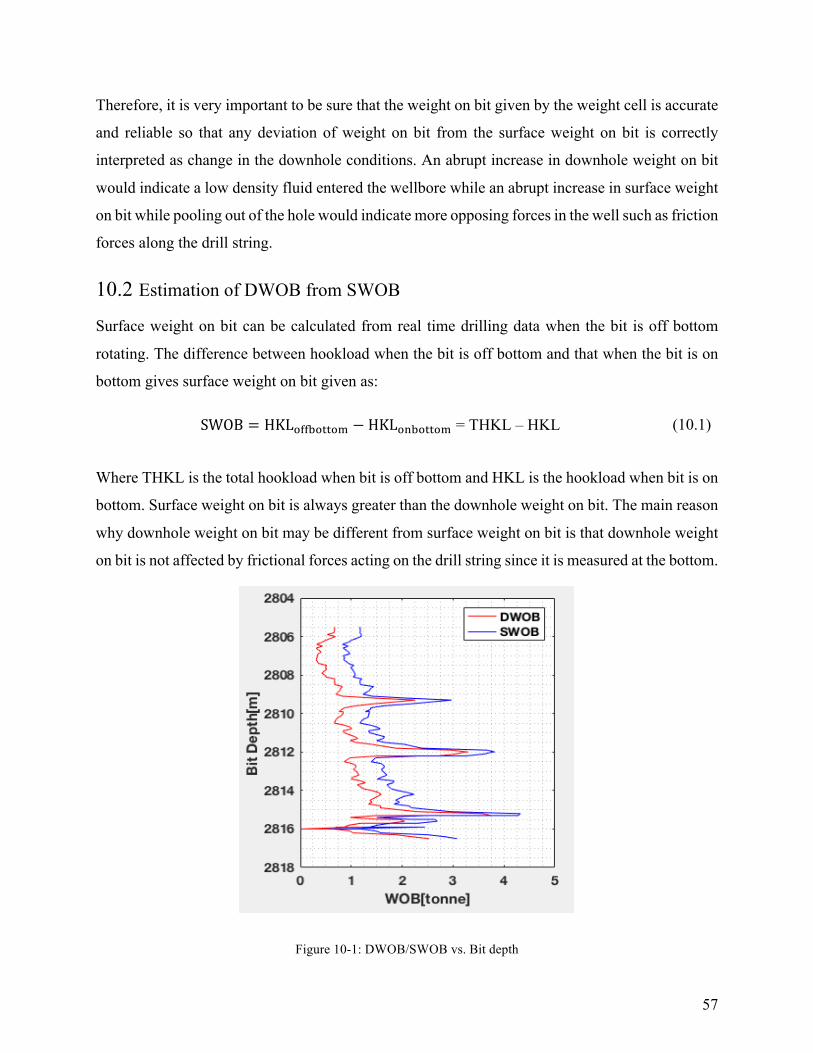
57
Therefore, it is very important to be sure that the weight on bit given by the weight cell is accurate
and reliable so that any deviation of weight on bit from the surface weight on bit is correctly
interpreted as change in the downhole conditions. An abrupt increase in downhole weight on bit
would indicate a low density fluid entered the wellbore while an abrupt increase in surface weight
on bit while pooling out of the hole would indicate more opposing forces in the well such as friction
forces along the drill string.
10.2! Estimation of DWOB from SWOB
Surface weight on bit can be calculated from real time drilling data when the bit is off bottom
rotating. The difference between hookload when the bit is off bottom and that when the bit is on
bottom gives surface weight on bit given as:
SWOB = HKL-ââ?-//-@ − HKL-*?-//-@ = THKL – HKL (10.1)
Where THKL is the total hookload when bit is off bottom and HKL is the hookload when bit is on
bottom. Surface weight on bit is always greater than the downhole weight on bit. The main reason
why downhole weight on bit may be different from surface weight on bit is that downhole weight
on bit is not affected by frictional forces acting on the drill string since it is measured at the bottom.
Figure 10-1: DWOB/SWOB vs. Bit depth

58
Figure 10-1 shows comparison between downhole and surface weight on bit for well 47-8-5. The
surface weight on bit was calculated from hookload values when the bit was on and off bottom
rotating. The results indicate that surface weight on bit is always greater than downhole weight on
bit. The trend increases down the hole and at some depths such as 2809m, 2812m and 2815m both
surface and downhole weight on bit increased rapidly. This may indicate change in bulk density at
the bottom around the BHA which led to increase in both DWOB and SWOB.
10.2.1! Converting SWOB into DWOB
Friction needs to be taken into account in order to accurately calculate downhole weight on bit
from the surface weight on bit so that the computed values match the measured downhole weight
values. This can be done using two approaches, the torque and drag model and the finite element
model. The torque and drag is simple and fast but does not give accurate results as finite element
does. In this thesis, only torque and drag model was used to analyze the steps needed to estimate
the downhole weight on bit under assumption that the wellbore section was straight. The torque
and drag model for a straight section is given by:
FÜ = βÜ wdLÜcos αi ± 7Õ wdLÜsin αi777 (10.2)
Where F) is the force at the top of element i and βÜ is the buoyancy factor on element i. The
second term in equation(10.2) is the frictional force, given by Fr = ÕwdLsin α) where Õ is the
coefficient of friction, w is the unit weight of the drill string element, dLÜ is its length and α) is
the inclination angle.
Equation(10.2) can be used to estimate the frictional forces and finally the coefficient of friction
using real time drilling data for when the bit is being pulled out of hole and when is being lowered
into the hole. The pull up force is given by F.A = βÜ wdLÜcos αi + 7Õ wdLÜsin αi and when
lowering into the well the force is given by FI-ø* = βÜ wdLÜcos αi − 7Õ wdLÜsin αi .
Combining the two equations for F.A and FI-ø* gives:
2ÕwdLÜsin α)7= Fr = 7F.A 7− 7FI-ø* (10.3)

59
Equation(10.3) can be converted into coefficient of friction as:
Õ7= ≥M°7]7≥N䟆7
åøI¿ΩD)* ‘Y (10.4)
Equation(10.3) gives the frictional force from hookload values when the string is pulled out and
when it is lowered into the well. This frictional force can be used to adjust the surface weight on
bit through iterations until the difference between the measured and calculated downhole weight
on bit is within acceptable range.
Table 10-2: RTDD during tripping operation for well 47-8-5
Hole!Depth!
Bit!Depth!
Motion!
WOB! HKL! RPM! SPP!
(m)! (m)! (tonne)! (tonne)! (rev/min)! (bar)!1579.8! 1579.3! On!bottom! 17.94! 83.78! 120.54! 146.81!
1579.8& 1578.8& Off!bottom! 0& 89.07& 120.4&148.07&
1579.8! 1578.1! up! 0! 90.65! 120.59! 147.68!1579.8! 1577.7! up! 0! 87.78! 120.6! 148.57!1579.8! 1577.2! up! 0! 87.24! 120.63! 148.56!1579.8! 1576.8! up! 0! 87.17! 120.65! 148.03!1579.8! 1573.5! up! 0! 89.43! 41.91! 2.38!1579.8! 1574! up! 0! 89.47! 42.11! 149.04!1579.8! 1574.6! down! 0! 89.45! 42.11! 98.26!1579.8! 1575! down! 0! 89.34! 42.09! 126.93!1579.8! 1576.4! down! 0! 89.23! 42.13! 143.92!1579.8! 1577.1! down! 0! 89.19! 42.17! 148.56!1579.8! 1579.8! On!bottom! 4.06! 89.12! 120.65! 147.75!
10.2.2! Steps in Calculating DWOB from SWOB
Table 10-2 shows real time drilling data when the drill string is off bottom. The frictional force for
this depth interval can be calculated using equation(10.3). In this case F.A= 90.65tonnes while
FI-ø*= 89.43tonnes and frictional force is FH =71.05tonnes. Also the off bottom and on bottom
hookload are 89.07 and 83.78tonnes respectively. This gives the surface weight on bit of

60
5.29tonnes while the downhole weight on bit is 4.06tonnes. This SWOB of 5.29tonnes is greater
than DWOB by 1.23tonnes. This value is also greater than the calculated frictional force which is
1.05tonnes. After that a coefficient of friction needs to be calculated using equation(10.4) to re –
estimate the new frictional force through iterations until when the surface weight on bit and
downhole weight on bit differ by the frictional force calculated from the difference between the
force during pulling up and the force during pulling down.
Figure 10-2: Measured and calculated downhole weight on bit
Figure 10-2 shows the estimated from RTDD for the depth interval of 2805m to 2814m. These
downhole weight on bit were calculated using the procedures described in 10.2.2 above. The
calculated DWOB matches the measured weight on bit with a small difference. It is shown that,

61
with all the small differences between the measured and calculated weight on bit values, the
general trend between the two data sets remains identical.
10.3! Mud Weight and Buoyancy Factor from DWOB
Bulk density of the mud can be calculated from downhole weight on bit calculated from real time
drilling data. The estimated DWOB is converted into buoyancy factor β given as:
βÜ 7= 77DWOBÜ7
wdLÜcos αi
(10.5)
Where βÜ and DWOBÜ are the buoyancy factor and downhole weight on bit
respectively at the kth bit depth. This buoyancy factor can be converted into bulk
density [email protected], of the mud just below the bit using: Where [email protected] is the bulk density
and rhoD/EEF7is density of steel.
[email protected] 7= (1 −7βÜ)rhoD/EEF77 (10.6)
Figure 10-3: Hookload, density and buoyancy factor calculated from DWOB

62
Figure 10-3 shows drilling parameters calculated from downhole weight on bit. The upper plot is
hookload calculated iteratively from downhole weight on bit. The lower plots present bulk density
and the corresponding buoyancy factor. The plots show how bulk density and buoyancy factor are
sensitive to change in hookload. Every time hookload changes leads to a corresponding change in
bulk density and buoyancy factor. However, in the upper plot, the calculated hookload is a bit large
than the measured hookload. This small discrepancy may be due to the torque and drag model
which was used to calculate downhole weight. Although this method is fast, its accuracy depends
on many assumptions like well geometry and hole condition. In this thesis, calculations of
hookload were based on assumptions that the selected depth interval was in a straight section
inclined at 30° and also friction and wall contact forces were ignored. For that reason, only friction
in the well was taken into account. This might have been the reason why calculated hookload
values were a bit greater than measured hookload values.

63
11.0!Conclusion and Recommendations
11.1! Conclusion
•! Mathematical kick models have been developed. Drilling parameters which can change
with changing downhole conditions have been investigated to show the dependence
between them. Mud weight and buoyancy factor have been found to depend on gas fraction,
cuttings concentration and temperature. Gas fraction in the mud has greater impact on mud
weight than any other parameter in bottomhole pressure reduction while cuttings have less
impact and normally leads to increase in mud weight.
•! Mathematical models taking into account well geometry and a realistic drill string
geometry were developed to estimate surface hookload. The Archimedes buoyancy model
and the Piston – force model were compared and both were found to give approximately
the same results although the Archimedes model was found to be more accurate.
•! Downhole weight on bit model was developed whose inputs were surface hookload to
calculate surface and downhole weight on bit. The calculated downhole weight on bit were
close to measured downhole weight on bit. Discrepancies between the calculated and
measured downhole weight on bit were due to use of the torque and drag model which is
less accurate due to being affected by friction in the well. Bulk density and buoyancy
factors calculated from downhole weight on bit were also found to sensitively change with
change in surface hookload.
•! Kick model based on downhole weight on bit would be more accurate and quick to give
information at the surface about change in downhole conditions since downhole weight on
bit gives a better estimate of mud weight because it is not affected by friction.
•! It is difficult to say that models developed meet all requirements of being used to accurately
predict the occurrence of a kick. The models were based on many assumptions and
simplifications. However, based on these facts the most critical parameters of kick
detection were established. A more general and realistic model which can take into account
all parameters at the same time need to be developed. This can be a more realistic and
accurate model to predict the presence of kick in the well.

64
11.2! Recommendations
•! Wellbore and drill string geometry should be taken into account when estimating downhole
weight on bit. Coefficient of friction should be accurately estimated in order to get correct
weight on bit from surface weight on bit.
•! Finite element method should be used to accurately estimate downhole weight on bit from
surface hookload values since it might be accurate than the analytical torque and drag
model. The model should be able to take into account the geometry of the wellbore.
•! Real time drilling data from different wells should be used to test the downhole weight on
bit model in order to validate the model.

65
References
Aadnøy, B. (2006) Mechanics of drilling. Aachen: Shaker Verlag, 196.
Aadnoy, B. S. & Djurhuus, J. (2008) Theory and Application of a New Generalized Model for Torque and Drag, 2008/1/1/. SPE: Society of Petroleum Engineers.
Aadnoy, B. S. & Huusgaard, P. P. (2002) Analytical Models for Design of Wellpath and BHA, 2002/1/1/. SPE: Society of Petroleum Engineers.
Aadnoy, B. S. & Kaarstad, E. (2006) Theory and Application of Buoyancy in Wells, 2006/1/1/. SPE: Society of Petroleum Engineers.
Aadnoy, B. S., Larsen, K. & Berg, P. C. (1999) Analysis of Stuck Pipe in Deviated Boreholes, 1999/1/1/. SPE: Society of Petroleum Engineers.
Bush, D. C. & Freeman, D. L. (1986) Drill Cuttings Porosity, Grain Density, And Permeability By Direct Laboratory Measurements And Their Relatability, 1986/1/1/. SPWLA: Society of Petrophysicists and Well-Log Analysts.
Farah, O. F. (2013) Directional well design, trajectory and survey calculations, with a case study in fiale, asal rift, djibouti, [Lecture]. Ministry of Energy and Natural Resources, unpublished.
Ford, J. T., Peden, J. M., Oyeneyin, M. B., Gao, E. & Zarrough, R. (1990) Experimental Investigation of Drilled Cuttings Transport in Inclined Boreholes, 1990/1/1/. SPE: Society of Petroleum Engineers.
Glomstad, T. S. (2012) Analysis of Hook load Signal to reveal the Causes of RestrictionsMaster's thesis. Norwegian University of Science and Technology, 4.6.201220.11.2016].
Goldsmith, R. (1972) Why gas cut mud is not always a serious problem. World Oil, 175(5), 51-+.
Gupta, V., Dhameliya, J. D. & Jain, S. (2013) Liquid Lift Dual Gradient Drilling in Deep Water: Early Kick Detection and Control, 2013/4/19/. SPE: Society of Petroleum Engineers.

66
Hollman, L., Haq, I., Christenson, C., Silva, T. P. d., Fayed, M. I. B., Thorn, N. & Geldof, W. (2016) Developing a MPD Operation Matrix – Case History, 2015/3/17/. SPE: Society of Petroleum Engineers.
Hovda, S. (2017) Semi-analytical models on axial motions of an oil-well drillstring, Part II: Deviated wellbores, S.P Andersens veg 15a, Trondheim Norway.
Jonathan Felipe Galdino, Gabriel Merhy de Oliveira, Admilson T. Franco & Negrão, C. O. R. (2013) Transient Mathematical Model for Well Kick During Drilling Operations
Kristensen, E. (2013) Model of Hook Load During Tripping OperationMaster's thesis. Norwegian University of Science and Technology, June19.11.2016].
Ling, K., He, J., Ge, J., Pei, P. & Shen, Z. (2015) A rigorous method to calculate the rising speed of gas kick. Journal of Petroleum Exploration and Production Technology, 5(1), 81-89.
Lockett, T. J., Richardson, S. M. & Worraker, W. J. (1993) The Importance of Rotation Effects for Efficient Cuttings Removal During Drilling, 1993/1/1/. SPE: Society of Petroleum Engineers.
McCann, R. C., Quigley, M. S., Zamora, M. & Slater, K. S. (1995) Effects of High-Speed Pipe Rotation on Pressures in Narrow Annuli.
Ozbayoglu, M. E., Saasen, A., Sorgun, M. & Svanes, K. (2008) Effect of Pipe Rotation on Hole Cleaning for Water-Based Drilling Fluids in Horizontal and Deviated Wells, 2008/1/1/. SPE: Society of Petroleum Engineers.
Rader, D. W., Bourgoyne, A. T., Jr. & Ward, R. H. (1975) Factors Affecting Bubble-Rise Velocity Of Gas Kicks.
Rommetveit, R., Fjelde, K. K., Aas, B., Day, N. F., Low, E. & Schwartz, D. H. (2003) Hpht well control; an integrated approach, Offshore Technology Conference. Offshore Technology Conference.
Saasen, A. (1998) Hole Cleaning During Deviated Drilling - The Effects of Pump Rate and Rheology, 1998/1/1/. SPE: Society of Petroleum Engineers.
Sifferman, T. R. & Becker, T. E. (1992) Hole Cleaning in Full-Scale Inclined Wellbores.

67
Skalle, P. (2015a) Drilling Fluid Engineering, 6th edition.
Skalle, P. (2015b) Pressure Control During Oil Well Drilling, 6th edition.
Skalle, P., Podio, A. L. & Tronvoll, J. (1991) Experimental Study of Gas Rise Velocity and tis Effect on Bottomhole Pressure in a Vertical Well Offshore Europe Conference. Aberdeen.
Stokka, S. I., Andersen, J. O., Freyer, J. & Welde, J. (1993) Gas Kick Warner - An Early Gas Influx Detection Method, 1993/1/1/. SPE: Society of Petroleum Engineers.
Strong, M. W. (1939) Mud Technique in Iran.
Swanson, B. W., Gardner, A. G., Brown, N. P. & Murray, P. J. (1997) Slimhole Early Kick Detection by Real-Time Drilling Analysis.
Velmurugan, N., Bansal, G. & Sharma, T. (2015) WellCON: Early Kick Detection System Extended to Kill Sheet, 2015/12/6/. IPTC: International Petroleum Technology Conference.
Wold, A. A. & Kummen, H. T. (2015) The effect of cuttings on annular pressure loss-An analysis of field data in the North SeaNTNU.
Wu, A. & Hareland, G. (2012) Calculation of Friction Coefficient And Downhole Weight On Bit With Finite Element Analysis of Drillstring, 2012/1/1/. ARMA: American Rock Mechanics Association.