key management ratios, 4th edition (0273707310)
TRANSCRIPT
0273707310_JACKET-NEW.indd 1 30/11/05 10:37:00

Key management ratios
WKMR_A01.QXD 11/24/05 12:53 PM Page i
In an increasingly competitive world, we believe it’s quality ofthinking that gives you the edge – an idea that opens newdoors, a technique that solves a problem, or an insight that
simply makes sense of it all. The more you know, the smarterand faster you can go.
That’s why we work with the best minds in business and financeto bring cutting-edge thinking and best learning practice to a
global market.
Under a range of leading imprints, including Financial TimesPrentice Hall, we create world-class print publications and
electronic products bringing our readers knowledge, skills andunderstanding, which can be applied whether studying or at work.
To find out more about Pearson Education publications, or tell us about the books you’d like to find, you can visit us at
www.pearsoned.co.uk
WKMR_A01.QXD 11/24/05 12:53 PM Page ii

Key management ratios
The clearest guide to the critical numbersthat drive your businessfourth edition
Ciaran Walsh
WKMR_A01.QXD 11/24/05 12:53 PM Page iii
PEARSON EDUCATION LIMITED
Edinburgh GateHarlow CM20 2JETel: +44 (0)1279 623623Fax: +44 (0)1279 431059Website: www.pearsoned.co.uk
First published 1996Second edition 1998Third edition 2003Fouth edition published in Great Britain 2006
© Ciaran Walsh 2006
The right of Ciaran Walsh to be identified as author of this work has been asserted by him inaccordance with the Copyright, Designs and Patents Act 1988.
ISBN-13: 978-0-273-70731-8ISBN-10: 0-273-70731-0
British Library Cataloguing-in-Publication DataA catalogue record for this book is available from the British Library
Library of Congress Cataloging-in-Publication Data
Walsh, Ciaran.Key management ratios : the clearest guide to the critical numbers that drive your
business / Ciaran Walsh.-- 4th ed.p. cm.
Includes index.ISBN-13: 978-0-273-70731-8 (alk. paper)ISBN-10: 0-273-70731-0 (alk. paper)1. Ratio analysis. 2. Management--Statistical methods. 3. Statistical decision. I. Title.
HF5681.R25W347 2006658.4’033--dc22
2005054680
All rights reserved. No part of this publication may be reproduced, stored in a retrievalsystem, or transmitted in any form or by any means, electronic, mechanical, photocopying,recording or otherwise, without either the prior written permission of the Publishers or alicence permitting restricted copying in the United Kingdom issued by the CopyrightLicensing Agency Ltd, 90 Tottenham Court Road, London W1T 4LP. This book may not belent, resold, hired out or otherwise disposed of by way of trade in any form of binding orcover other than that in which it is published, without the prior consent of the Publishers.
10 9 8 7 6 5 4 3 2 109 08 07 06 05
Typeset in Century Schoolbook by 30Printed and bound by Bell & Bain Limited, Glasgow
The Publishers’ policy is to use paper manufactured from sustainable forests.
WKMR_A01.QXD 11/24/05 12:53 PM Page iv

Ciaran Walsh is Senior Finance Specialist at the Irish ManagementInstitute, Dublin.
He is trained both as an economist and an accountant (BSc (Econ)London, CIMA) and had 15 years’ industrial experience before joining theacademic world.
His work with senior managers over many years has enabled him todevelop his own unique approach to training in corporate finance. As aconsequence, he has lectured in most European countries, the MiddleEast and Eastern Europe.
His main research interest is to identify and computerize the links thattie corporate growth and capital structure into stockmarket valuation.
He lives in Dublin and is married with six children.He can be contacted at [email protected]
About the author v
About the author
WKMR_A01.QXD 11/24/05 12:53 PM Page v

To our grandchildren
RebeccaIsobel
BenjaminEleanorSophie
EveHannaHollyGraceAaronAliceZoe
ImogenKate
Lei Xiao Shun
WKMR_A01.QXD 11/24/05 12:53 PM Page vi
Contents vii
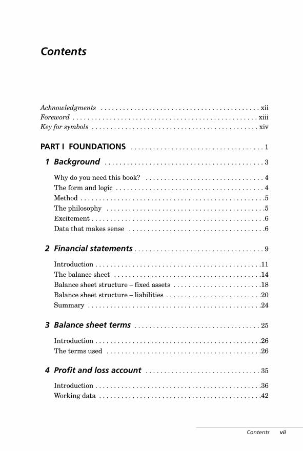
Acknowledgments . . . . . . . . . . . . . . . . . . . . . . . . . . . . . . . . . . . . . . . . . . . xiiForeword . . . . . . . . . . . . . . . . . . . . . . . . . . . . . . . . . . . . . . . . . . . . . . . . . . xiiiKey for symbols . . . . . . . . . . . . . . . . . . . . . . . . . . . . . . . . . . . . . . . . . . . . . xiv
PART I FOUNDATIONS . . . . . . . . . . . . . . . . . . . . . . . . . . . . . . . . . . . . 1
1 Background . . . . . . . . . . . . . . . . . . . . . . . . . . . . . . . . . . . . . . . . . . . 3
Why do you need this book? . . . . . . . . . . . . . . . . . . . . . . . . . . . . . . . . 4The form and logic . . . . . . . . . . . . . . . . . . . . . . . . . . . . . . . . . . . . . . . . 4Method . . . . . . . . . . . . . . . . . . . . . . . . . . . . . . . . . . . . . . . . . . . . . . . . . .5The philosophy . . . . . . . . . . . . . . . . . . . . . . . . . . . . . . . . . . . . . . . . . . .5Excitement . . . . . . . . . . . . . . . . . . . . . . . . . . . . . . . . . . . . . . . . . . . . . . .6Data that makes sense . . . . . . . . . . . . . . . . . . . . . . . . . . . . . . . . . . . . .6
2 Financial statements . . . . . . . . . . . . . . . . . . . . . . . . . . . . . . . . . . . 9
Introduction . . . . . . . . . . . . . . . . . . . . . . . . . . . . . . . . . . . . . . . . . . . . .11The balance sheet . . . . . . . . . . . . . . . . . . . . . . . . . . . . . . . . . . . . . . . .14Balance sheet structure – fixed assets . . . . . . . . . . . . . . . . . . . . . . . .18Balance sheet structure – liabilities . . . . . . . . . . . . . . . . . . . . . . . . . .20Summary . . . . . . . . . . . . . . . . . . . . . . . . . . . . . . . . . . . . . . . . . . . . . . .24
3 Balance sheet terms . . . . . . . . . . . . . . . . . . . . . . . . . . . . . . . . . . 25
Introduction . . . . . . . . . . . . . . . . . . . . . . . . . . . . . . . . . . . . . . . . . . . . .26The terms used . . . . . . . . . . . . . . . . . . . . . . . . . . . . . . . . . . . . . . . . . .26
4 Profit and loss account . . . . . . . . . . . . . . . . . . . . . . . . . . . . . . . 35
Introduction . . . . . . . . . . . . . . . . . . . . . . . . . . . . . . . . . . . . . . . . . . . . .36Working data . . . . . . . . . . . . . . . . . . . . . . . . . . . . . . . . . . . . . . . . . . . .42
Contents
WKMR_A01.QXD 11/24/05 12:53 PM Page vii
PART II OPERATING PERFORMANCE . . . . . . . . . . . . . . . . . . . . . . 47
5 Measures of performance . . . . . . . . . . . . . . . . . . . . . . . . . . . . 49
Relationships between the balance sheet and profit and loss account . . . . . . . . . . . . . . . . . . . . . . . . . . . . . . . . . . . . . . . . . . .50
The ratios ‘return on total assets’ and ‘return on equity’ . . . . . . . .52Balance sheet layouts . . . . . . . . . . . . . . . . . . . . . . . . . . . . . . . . . . . . .54
6 Operating performance . . . . . . . . . . . . . . . . . . . . . . . . . . . . . . 59
Return on investment (ROI) . . . . . . . . . . . . . . . . . . . . . . . . . . . . . . .61Return on equity (ROE) . . . . . . . . . . . . . . . . . . . . . . . . . . . . . . . . . . .62Return on total assets (ROTA) . . . . . . . . . . . . . . . . . . . . . . . . . . . . . .64Standards of operating performance . . . . . . . . . . . . . . . . . . . . . . . . .66
7 Performance drivers . . . . . . . . . . . . . . . . . . . . . . . . . . . . . . . . . . 81
Operating performance . . . . . . . . . . . . . . . . . . . . . . . . . . . . . . . . . . . .82Operating profit model . . . . . . . . . . . . . . . . . . . . . . . . . . . . . . . . . . . .88
PART III CORPORATE LIQUIDITY . . . . . . . . . . . . . . . . . . . . . . . . . . 95
8 Cash flow cycle . . . . . . . . . . . . . . . . . . . . . . . . . . . . . . . . . . . . . . . 97
Corporate liquidity . . . . . . . . . . . . . . . . . . . . . . . . . . . . . . . . . . . . . . .99The cash cycle . . . . . . . . . . . . . . . . . . . . . . . . . . . . . . . . . . . . . . . . . . 100Measures of liquidity – long and short analysis . . . . . . . . . . . . . . . 110
9 Liquidity . . . . . . . . . . . . . . . . . . . . . . . . . . . . . . . . . . . . . . . . . . . . 113
Short-term liquidity measures . . . . . . . . . . . . . . . . . . . . . . . . . . . . .115Current ratio . . . . . . . . . . . . . . . . . . . . . . . . . . . . . . . . . . . . . . . . . . .116Quick ratio . . . . . . . . . . . . . . . . . . . . . . . . . . . . . . . . . . . . . . . . . . . . .118Working capital to sales ratio . . . . . . . . . . . . . . . . . . . . . . . . . . . . . 120Working capital days . . . . . . . . . . . . . . . . . . . . . . . . . . . . . . . . . . . . 122
10 Financial strength . . . . . . . . . . . . . . . . . . . . . . . . . . . . . . . . . . . 125
Interest cover . . . . . . . . . . . . . . . . . . . . . . . . . . . . . . . . . . . . . . . . . . .126‘Debt to equity’ ratio (D/E) . . . . . . . . . . . . . . . . . . . . . . . . . . . . . . . .128Leverage . . . . . . . . . . . . . . . . . . . . . . . . . . . . . . . . . . . . . . . . . . . . . . .134Summary . . . . . . . . . . . . . . . . . . . . . . . . . . . . . . . . . . . . . . . . . . . . . .136
viii Contents
WKMR_A01.QXD 11/24/05 12:53 PM Page viii
11 Cash flow . . . . . . . . . . . . . . . . . . . . . . . . . . . . . . . . . . . . . . . . . . . 137
The cash flow statement . . . . . . . . . . . . . . . . . . . . . . . . . . . . . . . . . .139Sources and uses of funds – method . . . . . . . . . . . . . . . . . . . . . . . .140Opening and closing cash reconciliation . . . . . . . . . . . . . . . . . . . . .144Long and short analysis . . . . . . . . . . . . . . . . . . . . . . . . . . . . . . . . . .146Financial reporting standards . . . . . . . . . . . . . . . . . . . . . . . . . . . . .150
PART IV DETERMINANTS OF CORPORATE VALUE . . . . . . . . 153
12 Corporate valuation . . . . . . . . . . . . . . . . . . . . . . . . . . . . . . . . . 155
Introduction . . . . . . . . . . . . . . . . . . . . . . . . . . . . . . . . . . . . . . . . . . . .156Share values . . . . . . . . . . . . . . . . . . . . . . . . . . . . . . . . . . . . . . . . . . .158
13 Financial leverage and corporate valuation . . . . . . . . . . 175
Introduction . . . . . . . . . . . . . . . . . . . . . . . . . . . . . . . . . . . . . . . . . . . .176Financial leverage . . . . . . . . . . . . . . . . . . . . . . . . . . . . . . . . . . . . . . .176V chart . . . . . . . . . . . . . . . . . . . . . . . . . . . . . . . . . . . . . . . . . . . . . . . .178Market to book ratio . . . . . . . . . . . . . . . . . . . . . . . . . . . . . . . . . . . . .182
14 Growth . . . . . . . . . . . . . . . . . . . . . . . . . . . . . . . . . . . . . . . . . . . . . . 189
Growth . . . . . . . . . . . . . . . . . . . . . . . . . . . . . . . . . . . . . . . . . . . . . . . .190Analysis . . . . . . . . . . . . . . . . . . . . . . . . . . . . . . . . . . . . . . . . . . . . . . .194Growth equilibrium . . . . . . . . . . . . . . . . . . . . . . . . . . . . . . . . . . . . .196Application to acquisitions . . . . . . . . . . . . . . . . . . . . . . . . . . . . . . . .202
PART V MANAGEMENT DECISION-MAKING . . . . . . . . . . . . . 205
15 Cost, volume and price relationships . . . . . . . . . . . . . . . . 207
Introduction . . . . . . . . . . . . . . . . . . . . . . . . . . . . . . . . . . . . . . . . . . . .209Costing illustration . . . . . . . . . . . . . . . . . . . . . . . . . . . . . . . . . . . . . .210Contribution . . . . . . . . . . . . . . . . . . . . . . . . . . . . . . . . . . . . . . . . . . .214Break-even (B/E) . . . . . . . . . . . . . . . . . . . . . . . . . . . . . . . . . . . . . . . .220Contribution to sales percentage (CPS) . . . . . . . . . . . . . . . . . . . . . .226Summary . . . . . . . . . . . . . . . . . . . . . . . . . . . . . . . . . . . . . . . . . . . . . .240
Contents ix
WKMR_A01.QXD 11/24/05 12:53 PM Page ix
16 Investment ratios . . . . . . . . . . . . . . . . . . . . . . . . . . . . . . . . . . . . 241
Introduction . . . . . . . . . . . . . . . . . . . . . . . . . . . . . . . . . . . . . . . . . . . .243Project appraisal – the problem . . . . . . . . . . . . . . . . . . . . . . . . . . . .244Project appraisal – steps to a solution (1) . . . . . . . . . . . . . . . . . . . .246Project appraisal – steps to a solution (2) . . . . . . . . . . . . . . . . . . . .248Project appraisal – present value (PV) . . . . . . . . . . . . . . . . . . . . . . .250Project appraisal – internal rate of return (IRR) . . . . . . . . . . . . . .254Project appraisal – summary . . . . . . . . . . . . . . . . . . . . . . . . . . . . . .256
17 Shareholder value added (SVA) . . . . . . . . . . . . . . . . . . . . . 259
Introduction . . . . . . . . . . . . . . . . . . . . . . . . . . . . . . . . . . . . . . . . . . . .261Description . . . . . . . . . . . . . . . . . . . . . . . . . . . . . . . . . . . . . . . . . . . .262Approach to valuation (1) . . . . . . . . . . . . . . . . . . . . . . . . . . . . . . . . .266Approach to valuation (2) . . . . . . . . . . . . . . . . . . . . . . . . . . . . . . . . .268Value for the equity shareholders . . . . . . . . . . . . . . . . . . . . . . . . . .274Discount factor . . . . . . . . . . . . . . . . . . . . . . . . . . . . . . . . . . . . . . . . .276Terminal (continuing) value . . . . . . . . . . . . . . . . . . . . . . . . . . . . . . .286Complete model . . . . . . . . . . . . . . . . . . . . . . . . . . . . . . . . . . . . . . . . .288
18 Acquisition analysis . . . . . . . . . . . . . . . . . . . . . . . . . . . . . . . . . 291
Introduction . . . . . . . . . . . . . . . . . . . . . . . . . . . . . . . . . . . . . . . . . . . .293Financial profile of Alpha Inc. . . . . . . . . . . . . . . . . . . . . . . . . . . . . .294Financial profile of Beta Inc. . . . . . . . . . . . . . . . . . . . . . . . . . . . . . .296Acquisition – first offer . . . . . . . . . . . . . . . . . . . . . . . . . . . . . . . . . .298Acquisition impact on EPS . . . . . . . . . . . . . . . . . . . . . . . . . . . . . . . .300Shareholder effects – generalized . . . . . . . . . . . . . . . . . . . . . . . . . .302Summary of effects on shareholders . . . . . . . . . . . . . . . . . . . . . . . .308Revised offer . . . . . . . . . . . . . . . . . . . . . . . . . . . . . . . . . . . . . . . . . . .310Relative versus absolute values . . . . . . . . . . . . . . . . . . . . . . . . . . . .312SVA models – Alpha Inc. and Beta Inc. . . . . . . . . . . . . . . . . . . . . . .316Addendum . . . . . . . . . . . . . . . . . . . . . . . . . . . . . . . . . . . . . . . . . . . . .318
19 Integrity of accounting statements . . . . . . . . . . . . . . . . . . 321
Introduction . . . . . . . . . . . . . . . . . . . . . . . . . . . . . . . . . . . . . . . . . . . 323Where we focus attention . . . . . . . . . . . . . . . . . . . . . . . . . . . . . . . . 324Operating revenue enhancement . . . . . . . . . . . . . . . . . . . . . . . . . . .325
x Contents
WKMR_A01.QXD 11/24/05 12:53 PM Page x
Methods of revenue enhancement – fictitious sales . . . . . . . . . . . .328Revenue enhancement – clues for detection . . . . . . . . . . . . . . . . . .329Operating cost . . . . . . . . . . . . . . . . . . . . . . . . . . . . . . . . . . . . . . . . . .330The balance sheet . . . . . . . . . . . . . . . . . . . . . . . . . . . . . . . . . . . . . . .333The cash flow statement . . . . . . . . . . . . . . . . . . . . . . . . . . . . . . . . . .339
Appendix 1: Special items . . . . . . . . . . . . . . . . . . . . . . . . . . . . . . . . . . . .341Appendix 2: Companies used in the sample . . . . . . . . . . . . . . . . . . . . . .356Appendix 3: Full set of ratio charts from sample companies . . . . . . . . .359Appendix 4: Discounting and compounding tables . . . . . . . . . . . . . . . .376Glossary . . . . . . . . . . . . . . . . . . . . . . . . . . . . . . . . . . . . . . . . . . . . . . . . . .384Index . . . . . . . . . . . . . . . . . . . . . . . . . . . . . . . . . . . . . . . . . . . . . . . . . . . . .394
Contents xi
WKMR_A01.QXD 11/24/05 12:53 PM Page xi

xii Acknowledgments
I wish to express my deep gratitude to those who helped to bring aboutthis publication. To Richard Stagg of Financial Times Prentice Hall, whooriginated the concept and carried it through. To my friends and col-leagues: the late John O’Sullivan, who was an unequaled source ofreference on even the most esoteric subjects, and John Dinan, who re-started the motor after a blow-out.
I am grateful to the staff of the Irish Management Institute Libraryand Dublin Central Library for their unstinted provision of all the finan-cial data that I sought, including data from the Financial Times and ExtelFinancial Ltd, and to Geraldine McDonnell and Carol Fitzpatrick, whocheerfully coped with all the work of the section while the author was inseclusion.
Finally, I acknowledge the debt I owe to my fellow travellers: TomCullen; the late Des Hally; Diarmuid Moore; Martin Rafferty. Theyploughed the first furrows and sowed the seed.
Acknowledgments
WKMR_A01.QXD 11/24/05 12:53 PM Page xii
Foreword xiii
The subject of corporate finance is explored in a hundred books, most ofwhich have a formidable and forbidding aspect to them. They containpage after page of dense text interspersed with complex equations andobscure terminology.
The sheer volume of material and its method of presentation suggeststhat this is a subject that can be conquered only by the most hardy ofadventurers. However, the truth is that the sum and substance of thisarea of knowledge consists of a relatively small number of essential finan-cial measures by means of which we can appraise the success of anycommericial enterprise.
These measures are derived from relationships that exist between vari-ous financial parameters in the business. While each measure in itself issimple to calculate, comprehension lies not in how to do the calculationsbut in understanding what these results mean and how the resultsof different measures mesh together to give a picture of the health ofa company.
The first edition of this book set out to remove the obscurity and com-plexity so as to make the subject accessible to all business managers. Itturned out to be very successful.
In this fourth edition, the same basic structure and approach is used.However, the examples and the benchmark data have been updated andexpanded to make the book more relevant to a wider audience.
Data has been drawn from approximately 200 companies worldwide sothe results have very wide usage.
In the third edition, a new chapter was added (chapter 18) to illustrate howthe techniques used throughout the book can be used for the analysis of a pro-posed acquisition. It shows first how to value the two companies in relativeterms and then how to value them in absolute terms using an SVA approach.
SVA is an exciting new area of analysis that all managers will want tobecome familiar with because it is one that will have most impact on theirresponsibilities over the coming years.
In this fourth edition, a further chapter is added (chapter 19). This exam-ines the subject of the integrity of accounting statements, discusses whenand how integrity may be breached and suggests methods of detection.
Foreword
WKMR_A01.QXD 11/24/05 12:53 PM Page xiii
xiv Key for symbols
The following icons and the concepts they represent have been usedthroughout this book.
Thinkers
Checklist/summary
Example
Key idea
Definition
Action/taking note
Key for symbols
!
?
✓
☛
%
WKMR_A01.QXD 11/24/05 12:53 PM Page xiv

Part I Foundations
WKMR_CH01.QXD 11/24/05 12:15 PM Page 1

WKMR_CH01.QXD 11/24/05 12:15 PM Page 2
1 BackgroundWhy do you need this book?
· The form and logic · Method
· The philosophy · Excitement
· Data that makes sense
And all I ask is a tall ship And a star to steer her by. JOHN MASEFIELD (1878–1967)
WKMR_CH01.QXD 11/24/05 12:15 PM Page 3
4 Key management ratios
Why do you need this book?
Business ratios are the guiding stars for the management of enterprises;they provide their targets and standards. They are helpful to managers indirecting them towards the most beneficial long-term strategies as well astowards effective short-term decision-making.
Conditions in any business operation change day by day and, in thisdynamic situation, the ratios inform management about the most impor-tant issues requiring their immediate attention. By definition the ratiosshow the connections that exist between different parts of the business.They highlight the important interrelationships and the need for a properbalance between departments. A knowledge of the main ratios, therefore,will enable managers of different functions to work more easily togethertowards overall business objectives.
The common language of business is finance. Therefore, the mostimportant ratios are those that are financially based. The manager will,of course, understand that the financial numbers are only a reflection ofwhat is actually happening and that it is the reality not the ratios thatmust be managed.
The form and logic
This book is different from the majority of business books. You will seewhere the difference lies if you flip through the pages. It is not so much atext as a series of lectures captured in print – a major advantage of a goodlecture being the visual supports.
It is difficult and tedious to try to absorb a complex subject by readingstraight text only. Too much concentration is required and too great aload is placed on the memory. Indeed, it takes great perseverance to con-tinue on to the end of a substantial text. It also takes a lot of time, andspare time is the one thing that busy managers do not have in quantity.
Diagrams and illustrations, on the other hand, add great power, enhanc-ing both understanding and retention. They lighten the load and speed upprogress. Furthermore, there is an elegance and form to this subject thatcan only be revealed by using powerful illustrations.
Managers operating in today’s ever more complex world have to assimi-late more and more of its rules. They must absorb a lot of informationquickly. They need effective methods of communication. This is the logicbehind the layout of this book.
☛
WKMR_CH01.QXD 11/24/05 12:15 PM Page 4
Background 5
Method
There are many, many business ratios and each book on the subject givesa different set – or, at least, they look different.
We see a multitude of names, expressions and definitions, a myriad offinancial terms and relationships, and this is bewildering. Many whomake an attempt to find their way through the maze give up in despair.
The approach taken in this book is to ignore many ratios initially inorder to concentrate on the few that are vital. These few, perhaps 20 inall, will be examined in depth. The reason for their importance, theirmethod of calculation, the standards we should expect from them and,finally, their interrelationships will be explored. To use the analogy of theconstruction of a building, the steel frame will be put in place, the heavybeams will be hoisted into position and securely bolted together and onlywhen this powerful skeleton is secure, will we even think about addingthose extra rooms that might be useful. It is easy to bolt on as many sub-sidiary ratios as we wish once we have this very solid base.
The subject is noted for the multitude of qualifications and exceptionsto almost every rule. It is these that cause confusion, even though, quiteoften, they are unimportant to the manager. (They are there because theyhave an accounting or legal importance.) Here, the main part of the bookignores most of these, but the ones that matter are mentioned in theappendices. Many statements will be made that are 95 percent true – the5 percent that is left unsaid being of importance only to the specialist.
The philosophy
This golden rule cannot be overemphasized, and an understanding of itsimplications is vital to successful commercial operations. This is true forindividual managers as well as for whole communities.
All commercial enterprises use money as a raw material which they must pay for.Accordingly, they have to earn a return sufficient to meet these payments. Enterprisesthat continue to earn a return sufficient to pay the market rate for funds usually pros-per. Those enterprises that fail over a considerable period to meet this going marketrate usually do not survive – at least in the same form and under the same ownership.
!
WKMR_CH01.QXD 11/24/05 12:15 PM Page 5
Excitement
Not only is this subject important for the promotion of the economic well-being of individuals and society, it is also exciting – it has almost becomethe greatest sport. Business provides all the thrills and excitement thatcompetitive humankind craves. The proof of this is that the thrusts andcounter-thrusts of the entrepreneurs provide the headlines in our daily Press.
This book will link the return on financial resources into day-to-day oper-ating parameters of the business. It will give these skills to managers fromall backgrounds. The objective is that all the functions of production, mar-keting, distribution, etc. can exercise their specialist skills towards thecommon goal of financial excellence in their organizations.
Data that makes sense
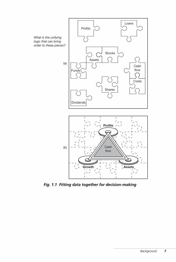
Managers, indeed, all of us, are deluged with business data. It comes frominternal operating reports, the daily Press, business magazines and manyother sources. Much of this data is incomprehensible. We know the mean-ing of the words used separately, but, used collectively, they can bemystifying. Figure 1.1 illustrates the problem. The individual words‘shares’, ‘profits’ and ‘cash flow’ are familiar to us, but we are not surehow they fit together to determine the viability of the business and arti-cles written about the subject are not much help – they seem to come upwith a new concept each month.
Is it possible to make the separate pieces shown in (a) into a coher-ent, comprehensive picture, as shown in (b)? The answer, for the mostpart, is ‘yes’.
The big issues in business are:
■ assets ■ profits ■ growth ■ cash flow.
These four variables have interconnecting links. There is a balance thatcan be maintained between them and, from this balance, will come corpo-rate value. It is corporate value that is the reason for most businessactivity and, for this reason, this book focuses on the business ratios thatdetermine corporate value.
6 Key management ratios
✓
WKMR_CH01.QXD 11/24/05 12:15 PM Page 6
Background 7
Fig. 1.1 Fitting data together for decision-making
Shares
Loans
Cashflow
Costs
Funds
Profits
Dividends
Assets
Stocks
(a)
(b) Cashflow
What is the unifyinglogic that can bringorder to these pieces?
Profits
Growth Assets
WKMR_CH01.QXD 11/24/05 12:15 PM Page 7

WKMR_CH01.QXD 11/24/05 12:15 PM Page 8
2 FinancialstatementsIntroduction · The balance sheet
· Balance sheet structure – fixed
assets · Balance sheet structure –
liabilities · Summary
Business is really a profession oftenrequiring for its practice quite as muchknowledge, and quite as much skill, aslaw and medicine; and requiring also thepossession of money.WALTER BAGEHOT (1826–1877)
WKMR_CH02.QXD 11/24/05 12:16 PM Page 9

WKMR_CH02.QXD 11/24/05 12:16 PM Page 10
Financial statements 11
Introduction
To have a coherent view of how a business performs, it is necessary, first,to have an understanding of its component parts. This job is not asformidable as it appears at first sight, because:
■ much of the subject is already known to managers, who will havecome in contact with many aspects of it in their work;
■ while there are, in all, hundreds of components, there are arelatively small number of vital ones;
■ even though the subject is complicated, it is based on common senseand can, therefore, be reasoned out once the ground rules havebeen established.
This last factor is often obscured by the language used. A lot of jargon isspoken and, while jargon has the advantage of providing a useful short-hand way of expressing ideas, it also has the effect of building an almostimpenetrable wall around the subject that excludes or puts off the non-specialist. I will leave it to the reader to decide for which purpose financialjargon is usually used, but one of the main aims here will be to show thecommon sense and logic that underlies all the apparent complexity.
Fundamental to this level of understanding is the recognition that, infinance, there are three – and only three – documents from which weobtain the raw data for our analysis. These are:
■ the balance sheet ■ the profit and loss account ■ the cash flow statement.
A description of each of these, together with their underlying logic, follows.
✓
WKMR_CH02.QXD 11/24/05 12:16 PM Page 11
12 Key management ratios
The balance sheet (B/S)
The balance sheet can be looked on as an engine with a certainmass/weight that generates power output in the form of profit. You willprobably remember from school the power/weight concept. It is a usefulanalogy here that demonstrates how a balance sheet of a given mass ofassets must produce a minimum level of profit to be efficient.
The profit and loss (P/L) account
The profit and loss account measures the gains or losses from bothnormal and abnormal operations over a period of time. It measures totalincome and deducts total cost. Both income and cost are calculatedaccording to strict accounting rules. The majority of these rules are obvi-ous and indisputable, but a small number are less so. Even thoughfounded on solid theory, they can sometimes, in practice, produce resultsthat appear ridiculous. While these accounting rules have always beensubject to review, recent events have precipitated a much closer examina-tion of them. Major changes are under way in the definition of such itemsas cash flow, subsidiary companies and so on.
The cash flow (C/F) statement
The statement of cash flow is a very powerful document. Cash flows intothe company when cheques are received and it flows out when chequesare issued, but an understanding of the factors that cause these flows isfundamental.
Summary
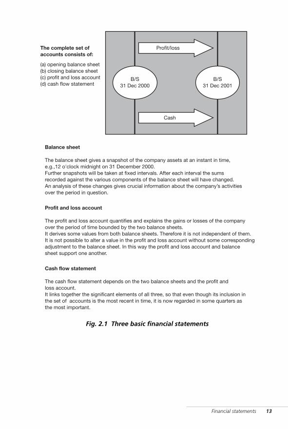
These three statements are not independent of each other, but are linkedin the system, as shown in figure 2.1. Together they give a full picture ofthe financial affairs of a business. We will look at each of these in greaterdetail.
But what is a balance sheet? It is simply an instant ‘snapshot’ of the assets usedby the company and of the funds that are related to those assets. It is a staticdocument relating to one point in time. We therefore take repeated ‘snapshots’at fixed intervals – months, quarters, years – to see how the assets and fundschange with the passage of time.
?
WKMR_CH02.QXD 11/24/05 12:16 PM Page 12
Financial statements 13
B/S31 Dec 2001
B/S31 Dec 2000
Cash
Profit/lossThe complete set ofaccounts consists of:
(a) opening balance sheet(b) closing balance sheet(c) profit and loss account(d) cash flow statement
Balance sheet
The balance sheet gives a snapshot of the company assets at an instant in time,e.g.,12 o'clock midnight on 31 December 2000.Further snapshots will be taken at fixed intervals. After each interval the sumsrecorded against the various components of the balance sheet will have changed.An analysis of these changes gives crucial information about the company’s activitiesover the period in question.
Profit and loss account
The profit and loss account quantifies and explains the gains or losses of the companyover the period of time bounded by the two balance sheets.It derives some values from both balance sheets. Therefore it is not independent of them.It is not possible to alter a value in the profit and loss account without some correspondingadjustment to the balance sheet. In this way the profit and loss account and balancesheet support one another.
Cash flow statement
The cash flow statement depends on the two balance sheets and the profit andloss account.It links together the significant elements of all three, so that even though its inclusion inthe set of accounts is the most recent in time, it is now regarded in some quarters asthe most important.
Fig. 2.1 Three basic financial statements
WKMR_CH02.QXD 11/24/05 12:16 PM Page 13
14 Key management ratios
The balance sheet
The balance sheet is the basic document of account. Traditionally it wasalways laid out as shown in figure 2.2, i.e., it consisted of two columnsthat were headed, respectively, ‘Liabilities’ and ‘Assets’. (Note that theword ‘Funds’ was often used together with or in place of ‘Liabilities’.)
The style now used is a single-column layout (see figure 5.3). This newlayout has some advantages, but it does not help the newcomer to under-stand the logic or structure of the document. For this reason, thetwo-column layout is mainly used in this publication.
Assets and liabilities
The ‘Assets’ column contains, simply, a list of items of value owned by thebusiness.
The ‘Liabilities’ column lists amounts due to parties external to the company,including the owners.
Assets are mainly shown in the accounts at their cost (or unexpired cost).Therefore the ‘Assets’ column is a list of items of value at their presentcost to the company. It can be looked on as a list of items of continuingvalue on which money has been used or spent.
The ‘Liabilities’ column simply lists the various sources of this samesum of money.
The amounts in these columns of course add up to the same total,because the company must identify exactly where funds were obtainedfrom to acquire the assets.
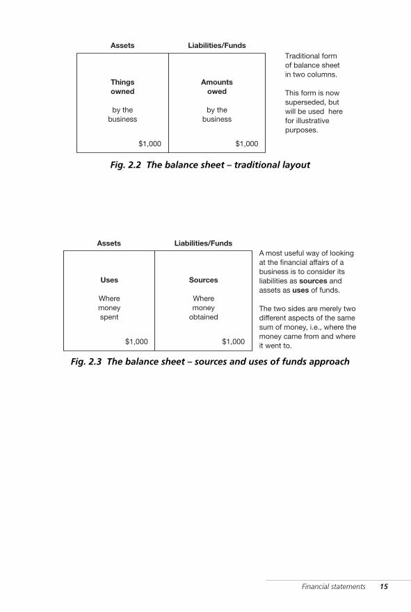
All cash brought into the business is a source of funds, while all cashpaid out is a use of funds. A balance sheet can, therefore, be looked onfrom this angle – as a statement of sources and uses of funds (see figure2.3). You will find it very helpful to bear this view of the balance sheet inmind as the theme is further developed (see chapter 11 for hidden itemsthat qualify this statement to some extent).
(The company is a legal entity separate from its owners, therefore, the term‘liability’ can be used in respect of amounts due from the company to its owners.)
?
WKMR_CH02.QXD 11/24/05 12:16 PM Page 14
Financial statements 15
Assets
Uses
Wheremoneyspent
Liabilities/Funds
Sources
Wheremoney
obtained
$1,000$1,000
A most useful way of lookingat the financial affairs of abusiness is to consider itsliabilities as sources andassets as uses of funds.
The two sides are merely twodifferent aspects of the samesum of money, i.e., where themoney came from and whereit went to.
Fig. 2.3 The balance sheet – sources and uses of funds approach
Assets
Thingsowned
by thebusiness
Liabilities/FundsTraditional formof balance sheetin two columns.
This form is nowsuperseded, butwill be used herefor illustrativepurposes.
Amountsowed
by thebusiness
$1,000$1,000
Fig. 2.2 The balance sheet – traditional layout
WKMR_CH02.QXD 11/24/05 12:16 PM Page 15
16 Key management ratios
Balance sheet structure
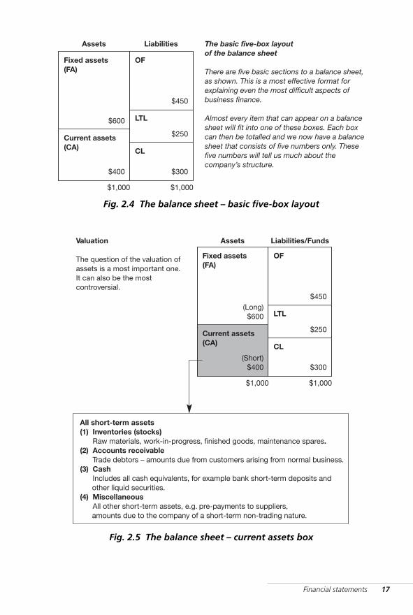
Figure 2.4 shows the balance sheet divided into five major blocks orboxes. These five subsections can accommodate practically all the itemsthat make up the total document. Two of these blocks are on the assetsside and three go to make up the liabilities side. We will continually comeback to this five-box structure, so it is worthwhile becoming comfortablewith it, as we go through each box in turn.
Let us look first at the two asset blocks. These are respectively called:
■ fixed assets (FA) ■ current assets (CA).
These can also be considered as ‘long’ and ‘short’ types of assets. We willsee that while this distinction is important in the case of assets, it is evenmore significant in the case of funds.
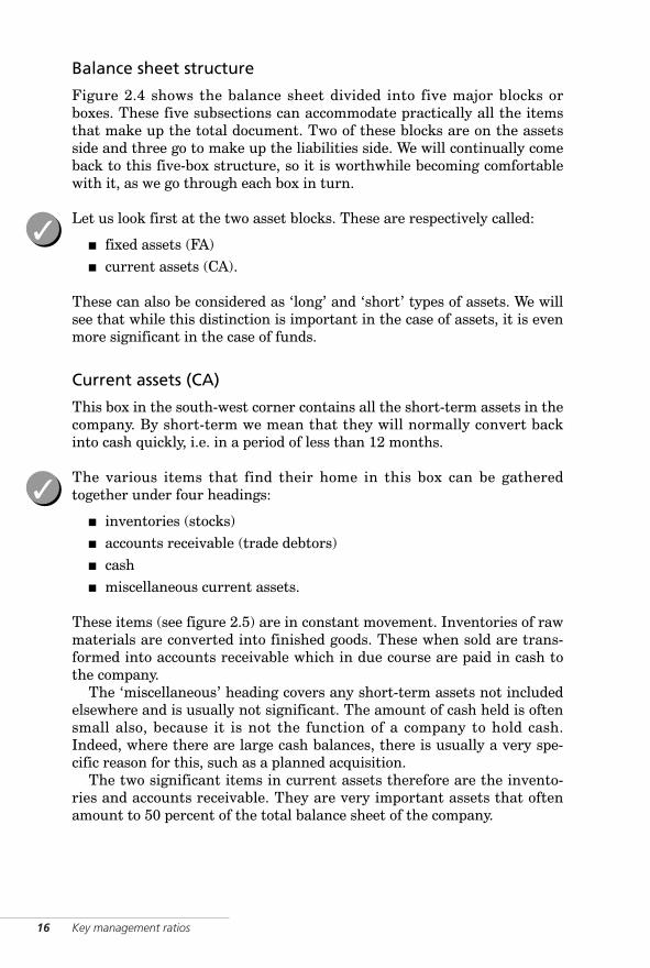
Current assets (CA)
This box in the south-west corner contains all the short-term assets in thecompany. By short-term we mean that they will normally convert backinto cash quickly, i.e. in a period of less than 12 months.
The various items that find their home in this box can be gatheredtogether under four headings:
■ inventories (stocks)■ accounts receivable (trade debtors) ■ cash■ miscellaneous current assets.
These items (see figure 2.5) are in constant movement. Inventories of rawmaterials are converted into finished goods. These when sold are trans-formed into accounts receivable which in due course are paid in cash tothe company.
The ‘miscellaneous’ heading covers any short-term assets not includedelsewhere and is usually not significant. The amount of cash held is oftensmall also, because it is not the function of a company to hold cash.Indeed, where there are large cash balances, there is usually a very spe-cific reason for this, such as a planned acquisition.
The two significant items in current assets therefore are the invento-ries and accounts receivable. They are very important assets that oftenamount to 50 percent of the total balance sheet of the company.
✓
✓
WKMR_CH02.QXD 11/24/05 12:16 PM Page 16
Financial statements 17
Liabilities/FundsAssetsValuation
The question of the valuation ofassets is a most important one.It can also be the mostcontroversial.
All short-term assets(1) Inventories (stocks)(1) Raw materials, work-in-progress, finished goods, maintenance spares.(2) Accounts receivable(1) Trade debtors – amounts due from customers arising from normal business.(3) Cash(1) Includes all cash equivalents, for example bank short-term deposits and(1) other liquid securities.(4) Miscellaneous(1) All other short-term assets, e.g. pre-payments to suppliers,(1) amounts due to the company of a short-term non-trading nature.
$1,000
Fixed assets(FA)
Current assets(CA)
OF
LTL
CL
$1,000
(Short)$400 $300
(Long)$600
$250
$450
Fig. 2.5 The balance sheet – current assets box
LiabilitiesAssets
$1,000
The basic five-box layoutof the balance sheet
There are five basic sections to a balance sheet,as shown. This is a most effective format forexplaining even the most difficult aspects ofbusiness finance.
Almost every item that can appear on a balancesheet will fit into one of these boxes. Each boxcan then be totalled and we now have a balancesheet that consists of five numbers only. Thesefive numbers will tell us much about thecompany’s structure.
Fixed assets(FA)
Current assets(CA)
OF
LTL
CL
$1,000
$400 $300
$600
$250
$450
Fig. 2.4 The balance sheet – basic five-box layout
WKMR_CH02.QXD 11/24/05 12:16 PM Page 17
18 Key management ratios
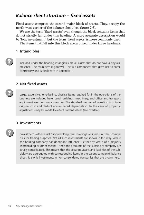
Balance sheet structure – fixed assets
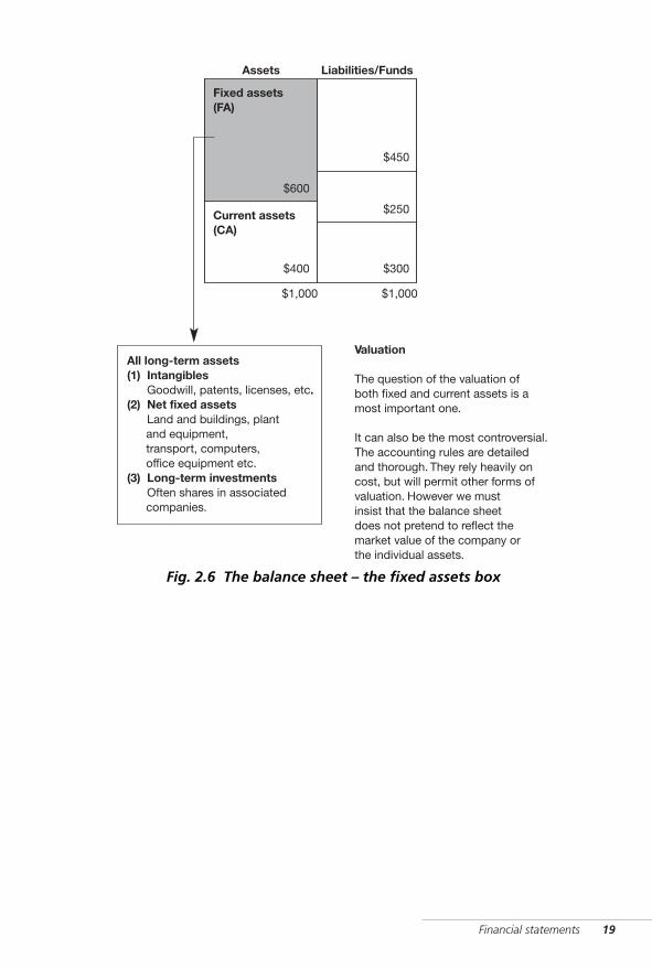
Fixed assets comprise the second major block of assets. They, occupy thenorth-west corner of the balance sheet (see figure 2.6).
We use the term ‘fixed assets’ even though the block contains items thatdo not strictly fall under this heading. A more accurate description wouldbe ‘long investment’, but the term ‘fixed assets’ is more commonly used.
The items that fall into this block are grouped under three headings:
1 Intangibles
2 Net fixed assets
3 Investments
‘Investments/other assets’ include long-term holdings of shares in other compa-nies for trading purposes. Not all such investments are shown in this way. Wherethe holding company has dominant influence – either by virtue of a majorityshareholding or other means – then the accounts of the subsidiary company aretotally consolidated. This means that the separate assets and liabilities of the sub-sidiary are aggregated with corresponding items in the parent company’s balancesheet. It is only investments in non-consolidated companies that are shown here.
?
Included under the heading intangibles are all assets that do not have a physicalpresence. The main item is goodwill. This is a component that gives rise to somecontroversy and is dealt with in appendix 1.
Large, expensive, long-lasting, physical items required for in the operations of thebusiness are included here. Land, buildings, machinery, and office and transportequipment are the common entries. The standard method of valuation is to takeoriginal cost and deduct accumulated depreciation. In the case of property,adjustments may be made to reflect current values (see overleaf).
?
?
WKMR_CH02.QXD 11/24/05 12:16 PM Page 18
Financial statements 19
Valuation
The question of the valuation ofboth fixed and current assets is amost important one.
It can also be the most controversial.The accounting rules are detailedand thorough. They rely heavily oncost, but will permit other forms ofvaluation. However we mustinsist that the balance sheetdoes not pretend to reflect themarket value of the company orthe individual assets.
All long-term assets(1) Intangibles(1) Goodwill, patents, licenses, etc.(2) Net fixed assets(1) Land and buildings, plant(1) and equipment,(1) transport, computers,(1) office equipment etc.(3) Long-term investments(1) Often shares in associated(1) companies.
Liabilities/FundsAssets
$1,000
Fixed assets(FA)
Current assets(CA)
$1,000
$400 $300
$600
$250
$450
Fig. 2.6 The balance sheet – the fixed assets box
WKMR_CH02.QXD 11/24/05 12:16 PM Page 19
20 Key management ratios
✓
The question as to whether the balance sheet values should be adjusted toreflect current market values has, for years, been a contentious question.In times of high inflation, property values get out of line – often consider-ably so – and it is recommended that they be revalued. However, it isimportant to note that the balance sheet does not attempt to reflect themarket value of either the separate assets or the total company.Prospective buyers or sellers of course examine these matters closely.
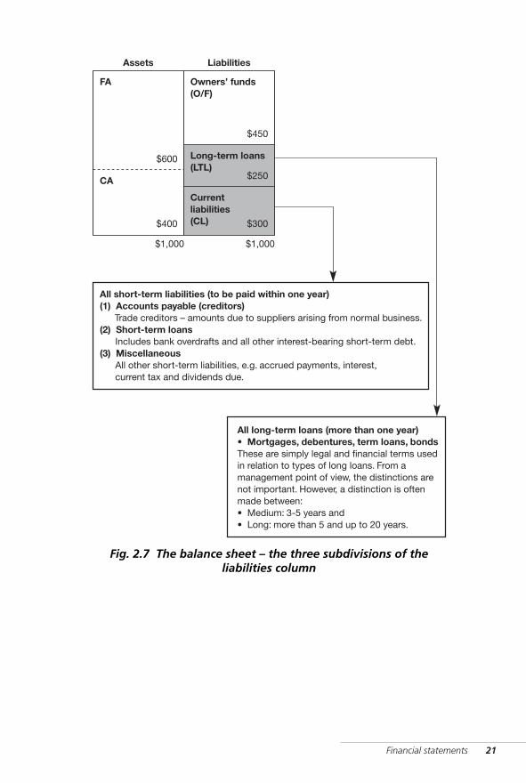
Balance sheet structure – liabilities
Figure 2.7 shows three subdivisions of the liabilities column:
■ owners’ funds (OF) ■ long-term loans (LTL) ■ current liabilities (CL).
(There are certain types of funds that do not fit comfortably into any oneof the above listed classes. At this stage we will ignore them. Usually theamounts are insignificant and they are dealt with in appendix 1).
Current liabilities (CL)
Current liabilities (see figure 2.7) have a strong parallel relationship withcurrent assets. ‘Accounts payable’ counterbalance ‘accounts receivable’,‘cash’ and ‘short-term loans’ reflect the day-to-day operating cash posi-tion at different stages. We will return to the relationship betweencurrent assets and current liabilities again.
Long-term loans (LTL)
These include mortgages, debentures, term loans, bonds, etc., that haverepayment terms longer than one year.
WKMR_CH02.QXD 11/24/05 12:16 PM Page 20
Financial statements 21
LiabilitiesAssets
All short-term liabilities (to be paid within one year)(1) Accounts payable (creditors)(1) Trade creditors – amounts due to suppliers arising from normal business.(2) Short-term loans(1) Includes bank overdrafts and all other interest-bearing short-term debt.(3) Miscellaneous(1) All other short-term liabilities, e.g. accrued payments, interest,(1) current tax and dividends due.
All long-term loans (more than one year)• Mortgages, debentures, term loans, bondsThese are simply legal and financial terms usedin relation to types of long loans. From amanagement point of view, the distinctions arenot important. However, a distinction is oftenmade between:• Medium: 3-5 years and• Long: more than 5 and up to 20 years.
$1,000
FA
CA
Owners’ funds(O/F)
Long-term loans(LTL)
Currentliabilities(CL)
$1,000
$400 $300
$600
$250
$450
Fig. 2.7 The balance sheet – the three subdivisions of theliabilities column
WKMR_CH02.QXD 11/24/05 12:16 PM Page 21

22 Key management ratios
Owners’ funds (OF)*
This is the most exciting section of the balance sheet. Included here areall claims by the owners on the business. Here is where fortunes are madeand lost. It is where entrepreneurs can exercise their greatest skills andwhere takeover battles are fought to the finish. Likewise it is the placewhere ‘financial engineers’ regularly come up with new schemes designedto bring ever-increasing returns to the brave. Unfortunately, it is also thearea where most confusing entries appear in the balance sheet.
For the newcomer to the subject the most important thing to remember isthat the total in the box is the figure that matters, not the breakdownbetween many different entries. We will discuss this section at length inchapter 12. It is important to note that while our discussions center onpublicly quoted companies, everything said applies equally strongly tonon-quoted companies. The rules of the game are the same for both.
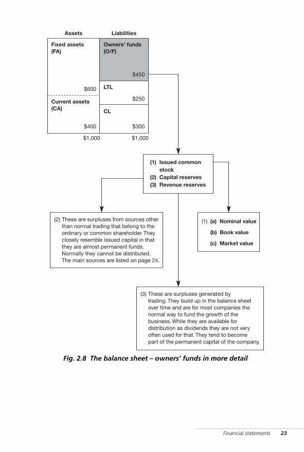
Note the three major subdivisions illustrated in figure 2.8:
■ issued common stock■ capital reserves ■ revenue reserves.
1 Issued common stock
The issuing of common stock for a cash consideration is the main mecha-nism for bringing owners’ capital into the business. Three differentvalues are associated with issued common stock:
■ nominal value ■ book value ■ market value.
These will be covered in detail in chapter 12.
* The terminology here is not easy. For this publication the following terms are identical:
■ owners’ funds
■ ordinary funds
■ common funds (US)
✓
WKMR_CH02.QXD 11/24/05 12:16 PM Page 22
Financial statements 23
LiabilitiesAssets
(2) (1)
(3)
(1) Issued common(1) stock(2) Capital reserves(3) Revenue reserves
$1,000
Fixed assets(FA)
Current assets(CA)
Owners’ funds(O/F)
LTL
CL
$1,000
$400 $300
$600
$250
$450
These are surpluses from sources otherthan normal trading that belong to theordinary or common shareholder. Theyclosely resemble issued capital in thatthey are almost permanent funds.Normally they cannot be distributed.The main sources are listed on page 24.
These are surpluses generated bytrading. They build up in the balance sheetover time and are for most companies thenormal way to fund the growth of thebusiness. While they are available fordistribution as dividends they are not veryoften used for that. They tend to becomepart of the permanent capital of the company.
(a) Nominal value
(b) Book value
(c) Market value
Fig. 2.8 The balance sheet – owners’ funds in more detail
WKMR_CH02.QXD 11/24/05 12:16 PM Page 23
2 Capital reserves
The heading ‘capital reserves’ is used to cover all surpluses accruing tothe common stockholders that have not arisen from trading. The mainsources of such funds are :
■ revaluation of fixed assets■ premiums on shares issued at a price in excess of nominal value ■ currency gains on balance sheet items, some non-trading profits, etc.
A significant feature of these reserves is that they cannot easily be paidout as dividends. In many countries there are also statutory reserveswhere companies are obliged by law to set aside a certain portion of trad-ing profit for specified purposes – generally to do with the health of thefirm. These are also treated as capital reserves.
3 Revenue reserves
These are amounts retained in the company from normal trading profit.Many different terms, names, descriptions can be attached to them:
■ revenue reserves ■ general reserve ■ retained earnings, etc.
This breakdown of revenue reserves into separate categories is unimpor-tant and the terms used are also unimportant. All the above items belongto the common stockholders. They have all come from the same sourceand they can be distributed as dividends to the shareholders at the will ofthe directors.
Summary
We use this five-box balance sheet for its clarity and simplicity. It will beseen later how powerful a tool it is for cutting through the complexities ofcorporate finance and explaining what business ratios really mean.
24 Key management ratios
WKMR_CH02.QXD 11/24/05 12:16 PM Page 24
3 Balance sheettermsIntroduction · The terms used
It sounds extraordinary but it’s a fact thatbalance sheets can make fascinating reading.MARY ARCHER (1989)
WKMR_CH03.QXD 11/24/05 12:17 PM Page 25

26 Key management ratios
Introduction
In order to understand and use business ratios we must be clear aboutwhat it is that is being measured. Definitions and terms used must be pre-cise and robust. We will define four terms each from the balance sheetand the profit and loss account. These are critical values in the accountsthat we come across all the time. In any discussion of company affairs,these terms turn up again and again, under many different guises andoften with different names. The five-box balance sheet layout will assistus greatly in this section.
The terms used
The four terms used in the balance sheet are very simple but important:
■ total assets ■ capital employed ■ net worth ■ working capital.
Each of these terms will be defined and illustrated in turn, with a furtherone introduced in chapter 17 (invested capital).
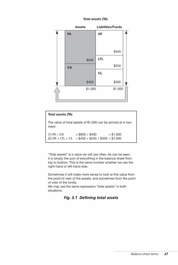
Total assets (TA)
You will see from figure 3.1 that the definition is straightforward:
TA = FA + CA$1,000 = $600 + $400
However, very often we use the term ‘total assets’ when we are reallymore interested in the right-hand side of the balance sheet where the def-inition more properly is:
TA = OF + LTL + CL$1,000 = $450 + $250 + $300
We must be able to see in our mind’s eye the relationship that existsbetween this and other balance sheet definitions.
NB: Sometimes we come across the term ‘total tangible assets’ (thematter of intangibles is discussed further in appendix 1).
✓
%
WKMR_CH03.QXD 11/24/05 12:17 PM Page 26
Balance sheet terms 27
Liabilities/FundsAssets
Total assets (TA)
The value of total assets of $1,000 can be arrived at in twoways:
(1) FA + CA(2) OF + LTL + CL
“Total assets” is a value we will use often. As can be seen,it is simply the sum of everything in the balance sheet fromtop to bottom. This is the same number whether we use theright-hand or left-hand side.
Sometimes it will make more sense to look at this value fromthe point of view of the assets, and sometimes from the pointof view of the funds.We may use the same expression “total assets” in bothsituations.
Total assets (TA)
= $600 + $400= $450 + $250 + $300
= $1,000= $1,000
$1,000
FA
CA
OF
LTL
CL
$1,000
$400 $300
$600
$250
$450
Fig. 3.1 Defining total assets
WKMR_CH03.QXD 11/24/05 12:17 PM Page 27
28 Key management ratios
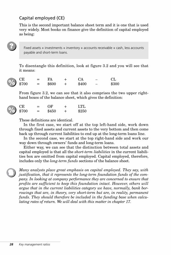
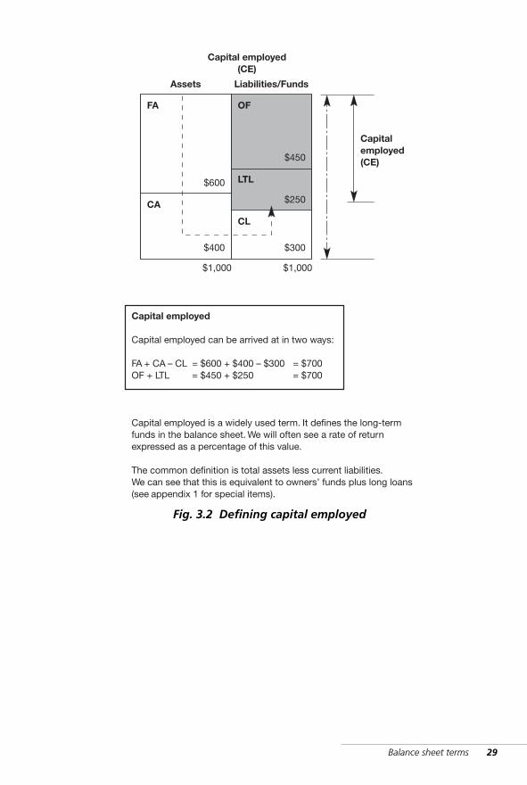
Capital employed (CE)
This is the second important balance sheet term and it is one that is usedvery widely. Most books on finance give the definition of capital employedas being:
To disentangle this definition, look at figure 3.2 and you will see thatit means:
CE = FA + CA – CL$700 = $600 + $400 – $300
From figure 3.2, we can see that it also comprises the two upper right-hand boxes of the balance sheet, which gives the definition:
CE = OF + LTL$700 = $450 + $250
These definitions are identical.In the first case, we start off at the top left-hand side, work down
through fixed assets and current assets to the very bottom and then comeback up through current liabilities to end up at the long-term loans line.
In the second case, we start at the top right-hand side and work ourway down through owners’ funds and long-term loans.
Either way, we can see that the distinction between total assets andcapital employed is that all the short-term liabilities in the current liabili-ties box are omitted from capital employed. Capital employed, therefore,includes only the long-term funds sections of the balance sheet.
Many analysts place great emphasis on capital employed. They say, withjustification, that it represents the long-term foundation funds of the com-pany. In looking at company performance they are concerned to ensure thatprofits are sufficient to keep this foundation intact. However, others willargue that in the current liabilities category we have, normally, bank bor-rowings that are, in theory, very short-term but are, in reality, permanentfunds. They should therefore be included in the funding base when calcu-lating rates of return. We will deal with this matter in chapter 17.
Fixed assets + investments + inventory + accounts receivable + cash, less accountspayable and short-term loans.
?
%
%
WKMR_CH03.QXD 11/24/05 12:17 PM Page 28
Balance sheet terms 29
Liabilities/FundsAssets
Capital employed(CE)
Capital employed
Capital employed can be arrived at in two ways:
FA + CA – CLOF + LTL
Capital employed is a widely used term. It defines the long-termfunds in the balance sheet. We will often see a rate of returnexpressed as a percentage of this value.
The common definition is total assets less current liabilities.We can see that this is equivalent to owners’ funds plus long loans(see appendix 1 for special items).
= $600 + $400 – $300= $450 + $250
= $700= $700
Capitalemployed(CE)
$1,000
FA
CA
OF
LTL
CL
$1,000
$400 $300
$600
$250
$450
Fig. 3.2 Defining capital employed
WKMR_CH03.QXD 11/24/05 12:17 PM Page 29
30 Key management ratios
!
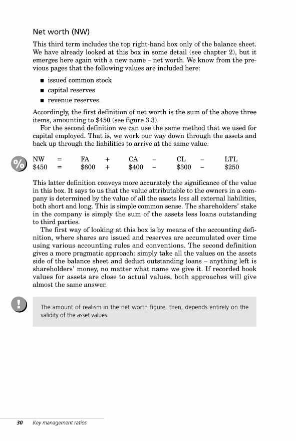
Net worth (NW)
This third term includes the top right-hand box only of the balance sheet.We have already looked at this box in some detail (see chapter 2), but itemerges here again with a new name – net worth. We know from the pre-vious pages that the following values are included here:
■ issued common stock ■ capital reserves ■ revenue reserves.
Accordingly, the first definition of net worth is the sum of the above threeitems, amounting to $450 (see figure 3.3).
For the second definition we can use the same method that we used forcapital employed. That is, we work our way down through the assets andback up through the liabilities to arrive at the same value:
NW = FA + CA – CL – LTL$450 = $600 + $400 – $300 – $250
This latter definition conveys more accurately the significance of the valuein this box. It says to us that the value attributable to the owners in a com-pany is determined by the value of all the assets less all external liabilities,both short and long. This is simple common sense. The shareholders’ stakein the company is simply the sum of the assets less loans outstandingto third parties.
The first way of looking at this box is by means of the accounting defi-nition, where shares are issued and reserves are accumulated over timeusing various accounting rules and conventions. The second definitiongives a more pragmatic approach: simply take all the values on the assetsside of the balance sheet and deduct outstanding loans – anything left isshareholders’ money, no matter what name we give it. If recorded bookvalues for assets are close to actual values, both approaches will givealmost the same answer.
%
The amount of realism in the net worth figure, then, depends entirely on thevalidity of the asset values.
WKMR_CH03.QXD 11/24/05 12:17 PM Page 30
Balance sheet terms 31
Net worth (NW)
The value of net worth is:
TA – CL – LTLOF (issued + c/reserves + r/reserves)
Net worthThis is another term often used to refer to the topright-hand box in the balance sheet.This box is such a significant section of the balance sheetthat it has many names attached to it.The term “net worth” has the advantage that it expressesthe fact that the value in this section is derived from:the total assets less the total external liabilities.
= $1,000 – $300 – $250 = $450= $450
Liabilities/FundsAssets
Net worth(NW)
TA
Issued sharesCapital reservesRevenue reserves
CE
Net worth(NW)
$1,000
FA
CA
OF
LTL
CL
$1,000
$400 $300
$600
$250
$450
Fig. 3.3 Defining net worth
WKMR_CH03.QXD 11/24/05 12:17 PM Page 31
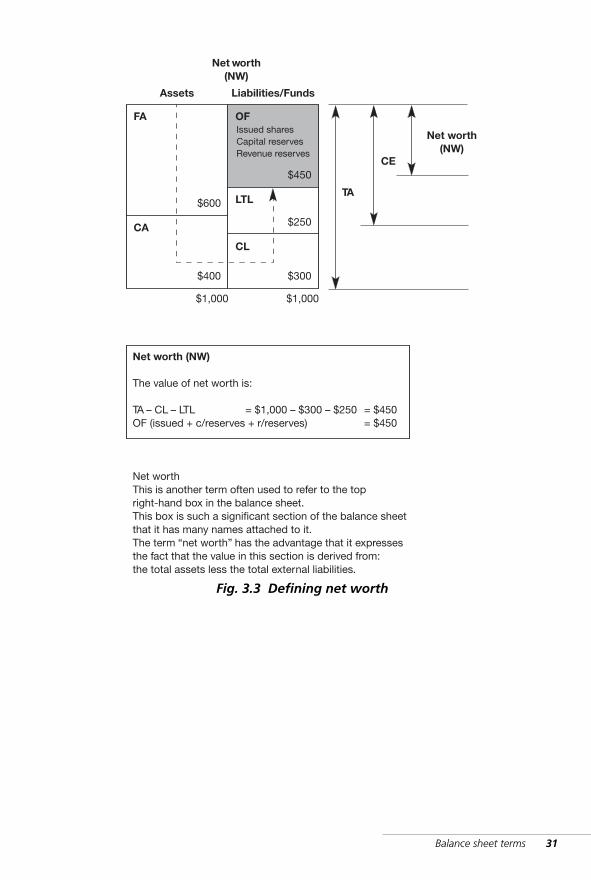
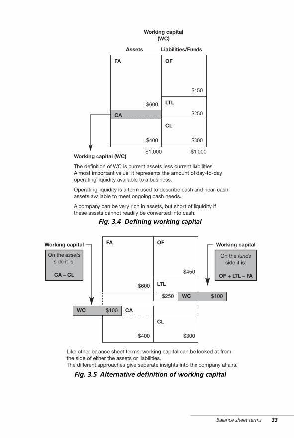
Working capital (WC)
This fourth and final balance sheet term is illustrated in figure 3.4. Itis an important term that we will come back to again and again in ourbusiness ratios.
The widely used definition of working capital is:
WC = CA – CL$100 = $400 – $300
This figure is a measure of liquidity. We can consider liquidity as an indi-cator of cash availability. It is clearly not the same thing as wealth: manypeople and companies who are very wealthy do not have a high degree ofliquidity. This happens if the wealth is tied up in assets that are not easilyconverted into cash. For instance, large farm and plantation owners havelots of assets, but may have difficulty in meeting day-to-day cash demands– they have much wealth but they are not liquid. This can be true forcompanies also. It is not sufficient to have assets; it is necessary to ensurethat there is sufficient liquidity to meet ongoing cash needs.
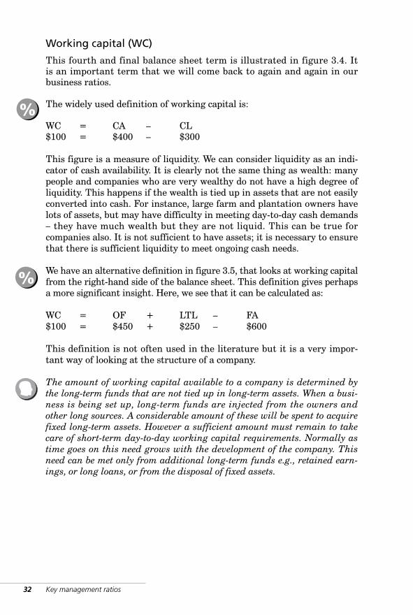
We have an alternative definition in figure 3.5, that looks at working capitalfrom the right-hand side of the balance sheet. This definition gives perhapsa more significant insight. Here, we see that it can be calculated as:
WC = OF + LTL – FA$100 = $450 + $250 – $600
This definition is not often used in the literature but it is a very impor-tant way of looking at the structure of a company.
The amount of working capital available to a company is determined bythe long-term funds that are not tied up in long-term assets. When a busi-ness is being set up, long-term funds are injected from the owners andother long sources. A considerable amount of these will be spent to acquirefixed long-term assets. However a sufficient amount must remain to takecare of short-term day-to-day working capital requirements. Normally astime goes on this need grows with the development of the company. Thisneed can be met only from additional long-term funds e.g., retained earn-ings, or long loans, or from the disposal of fixed assets.
32 Key management ratios
%
%
WKMR_CH03.QXD 11/24/05 12:17 PM Page 32
Balance sheet terms 33
Like other balance sheet terms, working capital can be looked at fromthe side of either the assets or liabilities.The different approaches give separate insights into the company affairs.
On the assetsside it is:
CA – CL
On the fundsside it is:
OF + LTL – FA
Working capital Working capitalFA
CA
OF
LTL
CL
$400 $300
$600
$250
$450
WC $100
WC $100
Fig. 3.5 Alternative definition of working capital
Liabilities/FundsAssets
Working capital (WC)
The definition of WC is current assets less current liabilities.A most important value, it represents the amount of day-to-dayoperating liquidity available to a business.
Operating liquidity is a term used to describe cash and near-cashassets available to meet ongoing cash needs.
A company can be very rich in assets, but short of liquidity ifthese assets cannot readily be converted into cash.
Working capital(WC)
$1,000
FA
CA
OF
LTL
CL
$1,000
$400 $300
$600
$250
$450
Fig. 3.4 Defining working capital
WKMR_CH03.QXD 11/24/05 12:17 PM Page 33

WKMR_CH03.QXD 11/24/05 12:17 PM Page 34
4 Profit and lossaccountIntroduction · Working data
A large income is the best recipe forhappiness I ever heard of.JANE AUSTEN (1775–1817)
WKMR_CH04.QXD 11/24/05 12:17 PM Page 35
36 Key management ratios
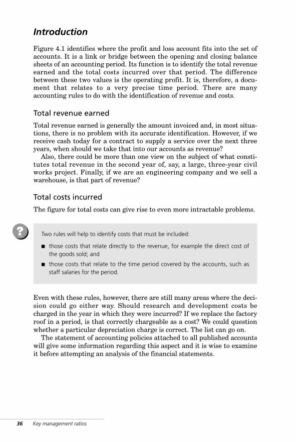
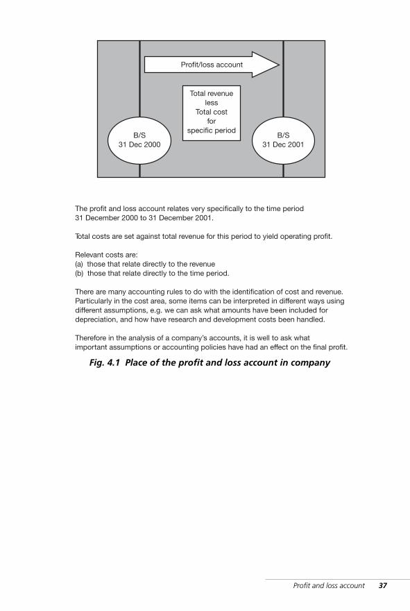
Introduction
Figure 4.1 identifies where the profit and loss account fits into the set ofaccounts. It is a link or bridge between the opening and closing balancesheets of an accounting period. Its function is to identify the total revenueearned and the total costs incurred over that period. The differencebetween these two values is the operating profit. It is, therefore, a docu-ment that relates to a very precise time period. There are manyaccounting rules to do with the identification of revenue and costs.
Total revenue earned
Total revenue earned is generally the amount invoiced and, in most situa-tions, there is no problem with its accurate identification. However, if wereceive cash today for a contract to supply a service over the next threeyears, when should we take that into our accounts as revenue?
Also, there could be more than one view on the subject of what consti-tutes total revenue in the second year of, say, a large, three-year civilworks project. Finally, if we are an engineering company and we sell awarehouse, is that part of revenue?
Total costs incurred
The figure for total costs can give rise to even more intractable problems.
Even with these rules, however, there are still many areas where the deci-sion could go either way. Should research and development costs becharged in the year in which they were incurred? If we replace the factoryroof in a period, is that correctly chargeable as a cost? We could questionwhether a particular depreciation charge is correct. The list can go on.
The statement of accounting policies attached to all published accountswill give some information regarding this aspect and it is wise to examineit before attempting an analysis of the financial statements.
Two rules will help to identify costs that must be included:
■ those costs that relate directly to the revenue, for example the direct cost ofthe goods sold; and
■ those costs that relate to the time period covered by the accounts, such asstaff salaries for the period.
?
WKMR_CH04.QXD 11/24/05 12:17 PM Page 36
Profit and loss account 37
The profit and loss account relates very specifically to the time period31 December 2000 to 31 December 2001.
Total costs are set against total revenue for this period to yield operating profit.
Relevant costs are:(a) those that relate directly to the revenue(b) those that relate directly to the time period.
There are many accounting rules to do with the identification of cost and revenue.Particularly in the cost area, some items can be interpreted in different ways usingdifferent assumptions, e.g. we can ask what amounts have been included fordepreciation, and how have research and development costs been handled.
Therefore in the analysis of a company’s accounts, it is well to ask whatimportant assumptions or accounting policies have had an effect on the final profit.
B/S31 Dec 2001
B/S31 Dec 2000
Profit/loss account
Total revenueless
Total costfor
specific period
Fig. 4.1 Place of the profit and loss account in company
WKMR_CH04.QXD 11/24/05 12:17 PM Page 37
38 Key management ratios
Profit and loss – general observations
In a situation where accountants can sometimes differ, it is not surprisingthat non-accounting managers go astray. One or two basic signposts willeliminate many problems that arise for the non-specialist in understand-ing this account.
The distinction between profit and cash flow is a common cause of con-fusion. The profit and loss account as such is not concerned with cashflow. This is covered by a separate statement. For instance, employees’pay incurred but not yet paid must be charged as cost even though therehas been no cash flow. On the other hand, payments to suppliers for goodsreceived are not costs, simply cash flow. Costs are incurred when goodsare consumed, not when they are purchased or paid for.
Cash spent on the purchase of assets is not a cost, but the correspon-ding depreciation over the following years is.
A loan repayment is not a cost because an asset (cash) and a liability(loan) are both reduced by the same amount, so there is no loss in valueby this transaction.
In recent years, the question of extraordinary items has been much dis-cussed. The issue here is whether large, one-off gains or losses should beincluded with normal trading activities. We can readily accept for analysispurposes the argument that these should be set to one side and not allowedto distort the normal operating results. This was the approach used in pro-ducing accounts for many years. However, in some companies, the rule wasused selectively. Items became extraordinary or otherwise in order to pres-ent the desired picture. The rule has now been changed to avoid thepossibility of distortion.
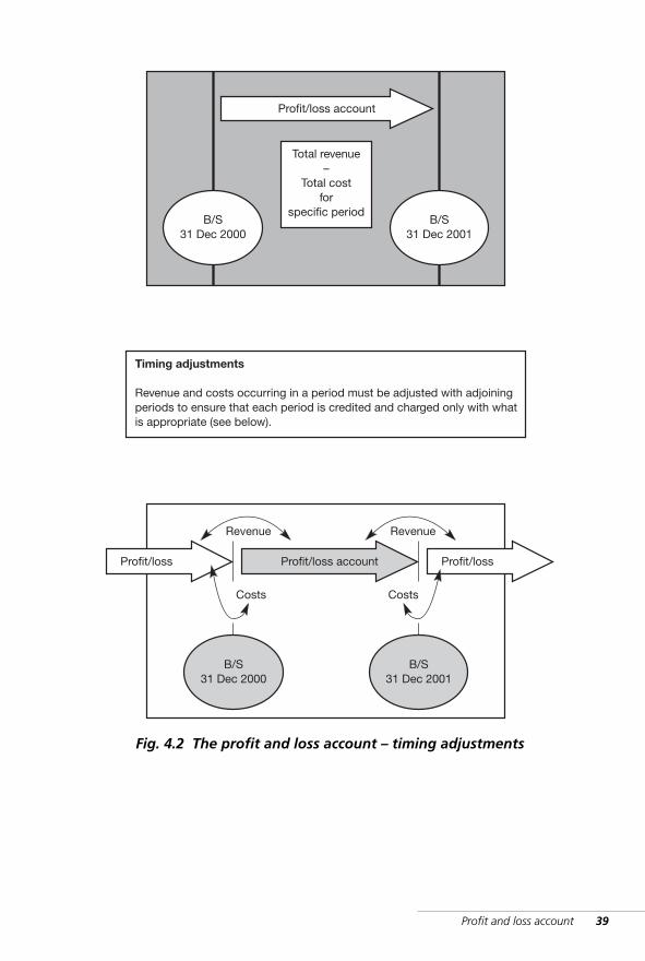
Finally the question of timing is vital. Having established what the true costs andrevenue are, we must locate them in the correct time period. The issue mainlyarises just before and just after the cut-off date between accounting periods. Asshown in figure 4.2, we may have to move revenue or costs forwards or back-wards to get them into their correct time periods.
!
WKMR_CH04.QXD 11/24/05 12:17 PM Page 38
Profit and loss account 39
B/S31 Dec 2001
B/S31 Dec 2000
Profit/loss account
Timing adjustments
Revenue and costs occurring in a period must be adjusted with adjoiningperiods to ensure that each period is credited and charged only with whatis appropriate (see below).
Total revenue–
Total costfor
specific period
B/S31 Dec 2001
B/S31 Dec 2000
Profit/loss accountProfit/loss Profit/loss
Costs Costs
Revenue Revenue
Fig. 4.2 The profit and loss account – timing adjustments
WKMR_CH04.QXD 11/24/05 12:17 PM Page 39
40 Key management ratios
Profit/loss – terms
Total revenue less total operating cost gives operating or trading profit.This is the first profit figure we encounter in the statements of accountbut there are many other definitions of profit.
We will identify four specific definitions and assign financial terms tothem. These are related to the way profit is distributed.
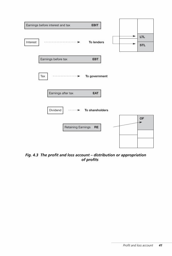
All the assets used in the business have played a part in generating theoperating profit to which we give the term ‘earnings before interest and tax(EBIT)’. Therefore this profit belongs to and must be distributed among thosewho have provided the assets. This is done according to well defined rules.
Figure 4.3 illustrates the process of distribution or ‘appropriation’ as itis called in the textbooks. There is a fixed order in the queue for distribu-tion as follows:
■ to the lenders (interest)■ to the taxation authorities (tax)■ to the shareholders (dividends/retentions).
At each of the stages of appropriation the profit remaining is given a pre-cise identification tag. Stripped of non-essentials, the following is a layoutof a standard profit and loss appropriation account. When looking at a setof accounts for the first time it may be difficult to see this structurebecause the form of layout is not as regular as we see in the balance sheet.However if one starts at the EBT figure, it is usually possible to work upand down to the other items shown:
■ EBIT – Earnings before interest and tax Deduct interest
■ EBT – Earnings before tax Deduct tax
■ EAT – Earnings after tax Deduct dividend
■ RE – Retained earnings
(See appendix 1 for further discussion of unusual items.)
✓
WKMR_CH04.QXD 11/24/05 12:17 PM Page 40
Profit and loss account 41
Earnings before interest and tax EBIT
Interest
Earnings before tax EBT
To lenders
Tax
Earnings after tax EAT
To government
Dividend
Retaining Earnings RE
To shareholders
LTL
STL
OF
Fig. 4.3 The profit and loss account – distribution or appropriation of profits
WKMR_CH04.QXD 11/24/05 12:17 PM Page 41
42 Key management ratios
Working data
Throughout the various stages of the book we will work with three setsof data:
■ The Example Co. plc has been devised with simple numbers tohighlight various aspects of accounts and show the calculation ofratios (see figure 4.4).
■ The US Consolidated Company Inc. (see figure 4.5).■ Sectoral/geographical data (see appendix 3).
The Example Company plc
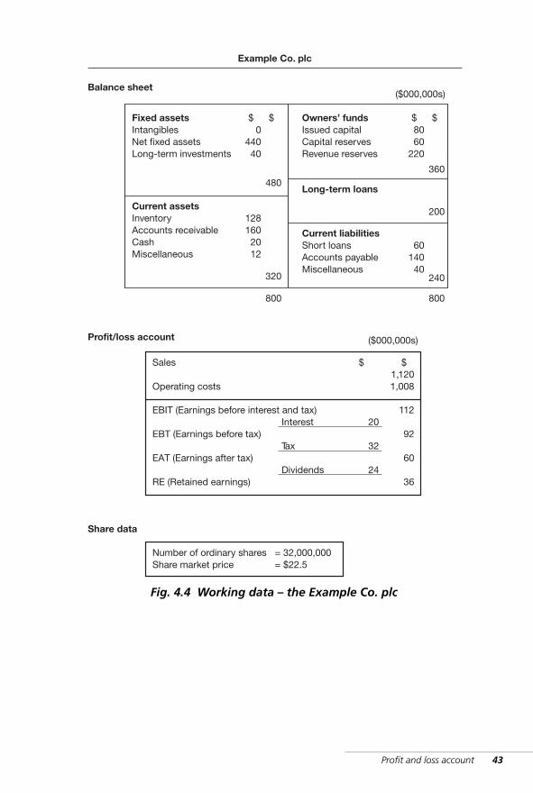
Figure 4.4 shows for the Example Company plc:
■ the balance sheet■ the profit/loss account■ share data.
It is worth while spending a moment looking over the now familiar five-box balance sheet and the structured profit/loss account to becomefamiliar with the figures. They will be used a lot in the following chapters.
Please review the following items:
Balance Sheet
■ Fixed assets ■ Current assets ■ Current liabilities ■ Long-term loans ■ Owners’ funds
Profit/Loss Account
■ EBIT Interest
■ EBT Tax
■ EAT Dividends
■ RE
✓
✓
WKMR_CH04.QXD 11/24/05 12:17 PM Page 42
Profit and loss account 43
Fixed assetsIntangiblesNet fixed assetsLong-term investments
Current assetsInventoryAccounts receivableCashMiscellaneous
Owners’ fundsIssued capitalCapital reservesRevenue reserves
Long-term loans
Current liabilitiesShort loansAccounts payableMiscellaneous
Sales
Operating costs
8060
220
$
360
$
200
6014040
240
800
044040
$
480
$
1281602012
320
800
Balance sheet
Profit/loss account
1,1201,008
$
EBIT (Earnings before interest and tax)
EBT (Earnings before tax)
EAT (Earnings after tax)
RE (Retained earnings)
Interest
Tax
Dividends
20
32
24
112
92
60
36
Number of ordinary sharesShare market price
= 32,000,000= $22.5
Share data
($000,000s)
$
Example Co. plc
($000,000s)
Fig. 4.4 Working data – the Example Co. plc
WKMR_CH04.QXD 11/24/05 12:17 PM Page 43
The US Consolidated Company Inc.
This company is made up of an aggregate of the accounts of approxi-mately 40 large successful US public companies drawn from differentbusiness sectors. These companies are flagships of US industry and theyhave been selected to provide aggregate data for the calculation of ratiosthat can be used as standards or norms for good industrial performance(see appendix 2).
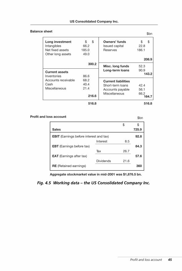
The balance sheet and profit/loss account for the year 2000 are laid outaccording to our agreed structure in figure 4.5. We will use these for set-ting targets of performance.
The aggregate stockmarket value of these companies in mid-2001 was$1,876.5 bn.
Sectoral/geographical data
In addition to the above, almost 200 high-profit companies from differentbusiness sectors and four geographic areas have been selected to indicatethe types of variation that arise in different types of operation in differentlocations. These business sectors are:
■ health care■ food■ machinery and equipment■ retail.
The locations are:
■ US■ UK■ EU■ Japan.
This produces 16 subgroups for which results are compared and reportedin graphical form throughout the book.
44 Key management ratios
WKMR_CH04.QXD 11/24/05 12:17 PM Page 44
Profit and loss account 45
Long investmentIntangiblesNet fixed assetsOther long assets
Current assetsInventoriesAccounts receivableCashMiscellaneous
Owners’ fundsIssued capitalReserves
Misc. long fundsLong-term loans
Current liabilitiesShort-term loansAccounts payableMiscellaneous
Sales
22.8186.1
$
208.9
$
143.2
42.456.166.2
164.7
516.8
66.2185.049.0
$
300.2
$
86.668.240.421.4
216.6
516.8
Balance sheet
Profit and loss account
725.9$
EBIT (Earnings before interest and tax)
EBT (Earnings before tax)
EAT (Earnings after tax)
RE (Retained earnings)
Interest
Tax
Dividends
8.5
26.7
21.6
92.8
84.3
57.6
360
$bn
$
US Consolidated Company Inc.
$bn
52.390.9
Aggregate stockmarket value in mid-2001 was $1,876.5 bn.
Fig. 4.5 Working data – the US Consolidated Company Inc.
WKMR_CH04.QXD 11/24/05 12:17 PM Page 45

WKMR_CH04.QXD 11/24/05 12:17 PM Page 46
Part II Operating performance
WKMR_CH05.QXD 11/24/05 12:18 PM Page 47

WKMR_CH05.QXD 11/24/05 12:18 PM Page 48
5 Measures ofperformanceRelationships between the
balance sheet and profit and loss
account · The ratios ‘return on
total assets’ and ‘return on equity’
· Balance sheet layouts
I often wonder what the vintners buy one thatis half so precious as the goods they sell.RUBAIYAT OF OMER KHAYYAM (1859)
WKMR_CH05.QXD 11/24/05 12:18 PM Page 49
50 Key management ratios
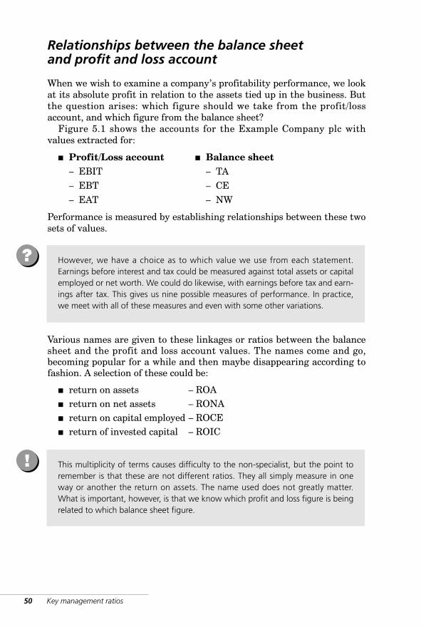
Relationships between the balance sheet and profit and loss account
When we wish to examine a company’s profitability performance, we lookat its absolute profit in relation to the assets tied up in the business. Butthe question arises: which figure should we take from the profit/lossaccount, and which figure from the balance sheet?
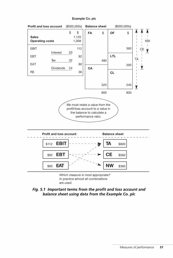
Figure 5.1 shows the accounts for the Example Company plc withvalues extracted for:
■ Profit/Loss account ■ Balance sheet– EBIT – TA– EBT – CE– EAT – NW
Performance is measured by establishing relationships between these twosets of values.
Various names are given to these linkages or ratios between the balancesheet and the profit and loss account values. The names come and go,becoming popular for a while and then maybe disappearing according tofashion. A selection of these could be:
■ return on assets – ROA■ return on net assets – RONA■ return on capital employed – ROCE■ return of invested capital – ROIC
However, we have a choice as to which value we use from each statement.Earnings before interest and tax could be measured against total assets or capitalemployed or net worth. We could do likewise, with earnings before tax and earn-ings after tax. This gives us nine possible measures of performance. In practice,we meet with all of these measures and even with some other variations.
?
This multiplicity of terms causes difficulty to the non-specialist, but the point toremember is that these are not different ratios. They all simply measure in oneway or another the return on assets. The name used does not greatly matter.What is important, however, is that we know which profit and loss figure is beingrelated to which balance sheet figure.
!
WKMR_CH05.QXD 11/24/05 12:18 PM Page 50
Measures of performance 51
SalesOperating costs
Profit and loss account
1,1201,008
$
EBIT
EBT
EAT
RE
Interest
Tax
Dividends
20
32
24
112
92
60
36
800800
FA
CA
OF
LTL
CL
240320
200
360
480
Balance sheet ($000,000s)
$$$
($000,000s)
We must relate a value from theprofit/loss account to a value in
the balance to calculate aperformance ratio.
Profit and loss account Balance sheet
EBIT
EBT
EAT
TA
CE
NW
Which measure is most appropriate?In practice almost all combinationsare used.
$112
$92
$60
$800
$560
$360
Example Co. plc
TA
CE
NW
Fig. 5.1 Important terms from the profit and loss account andbalance sheet using data from the Example Co. plc
WKMR_CH05.QXD 11/24/05 12:18 PM Page 51
52 Key management ratios
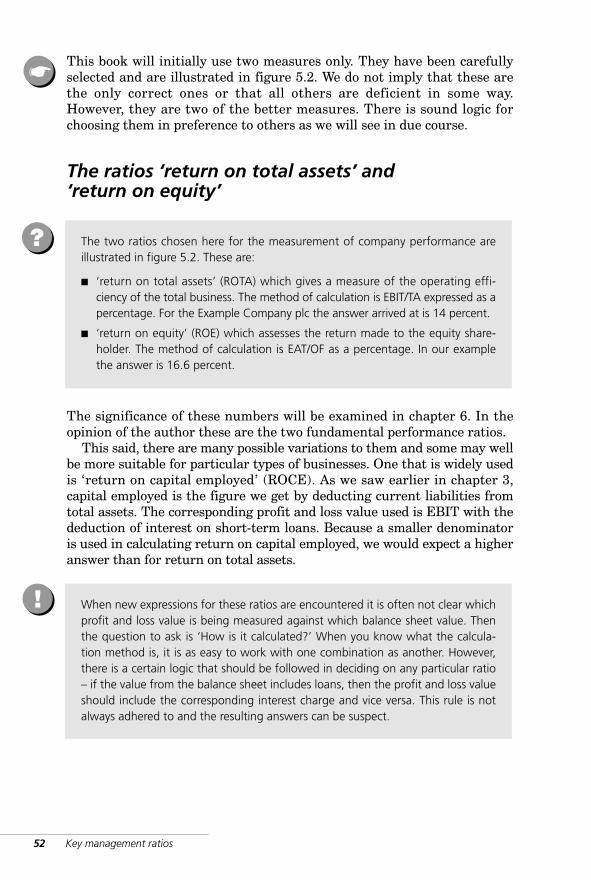
This book will initially use two measures only. They have been carefullyselected and are illustrated in figure 5.2. We do not imply that these arethe only correct ones or that all others are deficient in some way.However, they are two of the better measures. There is sound logic forchoosing them in preference to others as we will see in due course.
The ratios ‘return on total assets’ and ‘return on equity’
The significance of these numbers will be examined in chapter 6. In theopinion of the author these are the two fundamental performance ratios.
This said, there are many possible variations to them and some may wellbe more suitable for particular types of businesses. One that is widely usedis ‘return on capital employed’ (ROCE). As we saw earlier in chapter 3,capital employed is the figure we get by deducting current liabilities fromtotal assets. The corresponding profit and loss value used is EBIT with thededuction of interest on short-term loans. Because a smaller denominatoris used in calculating return on capital employed, we would expect a higheranswer than for return on total assets.
☛
The two ratios chosen here for the measurement of company performance areillustrated in figure 5.2. These are:
■ ‘return on total assets’ (ROTA) which gives a measure of the operating effi-ciency of the total business. The method of calculation is EBIT/TA expressed as apercentage. For the Example Company plc the answer arrived at is 14 percent.
■ ‘return on equity’ (ROE) which assesses the return made to the equity share-holder. The method of calculation is EAT/OF as a percentage. In our examplethe answer is 16.6 percent.
?
When new expressions for these ratios are encountered it is often not clear whichprofit and loss value is being measured against which balance sheet value. Thenthe question to ask is ‘How is it calculated?’ When you know what the calcula-tion method is, it is as easy to work with one combination as another. However,there is a certain logic that should be followed in deciding on any particular ratio– if the value from the balance sheet includes loans, then the profit and loss valueshould include the corresponding interest charge and vice versa. This rule is notalways adhered to and the resulting answers can be suspect.
!
WKMR_CH05.QXD 11/24/05 12:18 PM Page 52
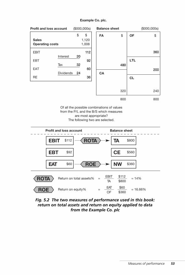
Measures of performance 53
Of all the possible combinations of valuesfrom the P/L and the B/S which measures
are most appropriate?The following two are selected.
Profit and loss account Balance sheet
EBIT
EBT
EAT
TA
CE
NW
ROTA
ROE
ROTA
ROE
Return on total assets% = EBITTA
$112$800
= 14%
Return on equity% = EATOF
$60$360
= 16.66%
$112
$92
$60
$800
$560
$360
SalesOperating costs
Profit and loss account
1,1201,008
$
20
32
24
112
92
60
36
800800
FA
CA
OF
CL
240320
200
360
480
Balance sheet ($000,000s)
$$$
($000,000s)
Example Co. plc.
EBIT
EBT
EAT
RE
Interest
Tax
Dividends
20
32
24
112
92
60
36
LTL
200
360
480
Fig. 5.2 The two measures of performance used in this book:return on total assets and return on equity applied to data
from the Example Co. plc
WKMR_CH05.QXD 11/24/05 12:18 PM Page 53
54 Key management ratios
Balance sheet layouts
A number of alternative forms of layout, particularly in the case of thebalance sheet, are used in presenting accounts. While the layout itselfdoes not affect any of the numbers, it can be difficult when faced with anunfamiliar format to find where items are located and what are values for‘total assets’, ‘capital employed’, etc.
The first point to remember is that the items within each of the fiveboxes will always appear grouped together – they are never scatteredaround among other items. Sometimes, however, the total only of a sub-section will appear in the balance sheet proper while the detail is to befound in the notes to accounts.
Vertical balance sheet – version 1
Given the five-box grouping, it follows that there is only a limited numberof ways in which the boxes can be arranged. In figure 5.3, one such re-arrangement is shown. It is easy to see how the items in the two-columnformat have been re-ordered into a single vertical column. This type oflayout has the advantage that corresponding values for successive yearscan be laid out side by side for ease of comparison. In this format, valuesfor ‘total assets’ and ‘total funds’ are also emphasized.
WKMR_CH05.QXD 11/24/05 12:18 PM Page 54
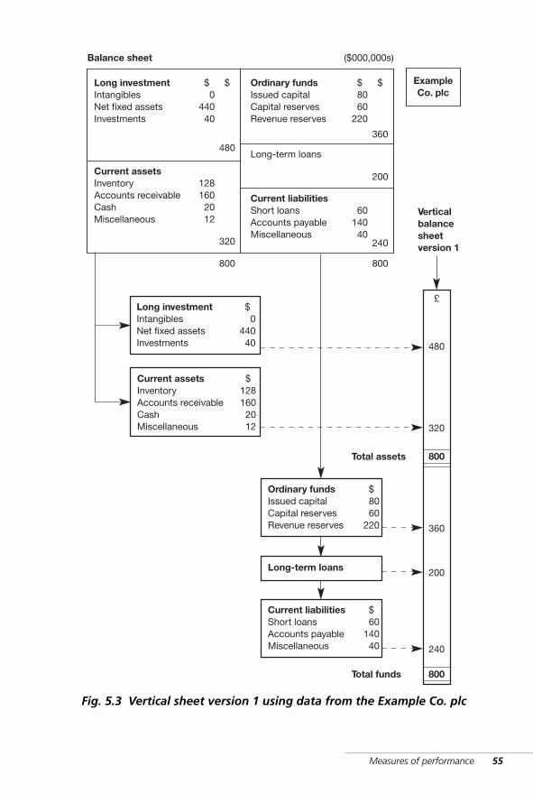
Measures of performance 55
Long investmentIntangiblesNet fixed assetsInvestments
044040
$
Current assetsInventoryAccounts receivableCashMiscellaneous
$1281602012
Ordinary fundsIssued capitalCapital reservesRevenue reserves
8060
220
$
Long-term loans
Current liabilitiesShort loansAccounts payableMiscellaneous
6014040
$
Verticalbalancesheetversion 1
£
480
Total assets
Total funds
320
800
360
200
240
800
Long investmentIntangiblesNet fixed assetsInvestments
Current assetsInventoryAccounts receivableCashMiscellaneous
Ordinary fundsIssued capitalCapital reservesRevenue reserves
Long-term loans
Current liabilitiesShort loansAccounts payableMiscellaneous
8060
220
$
360
$
200
6014040
240
800
044040
$
480
$
1281602012
320
800
Balance sheet ($000,000s)
ExampleCo. plc
Fig. 5.3 Vertical sheet version 1 using data from the Example Co. plc
WKMR_CH05.QXD 11/24/05 12:18 PM Page 55
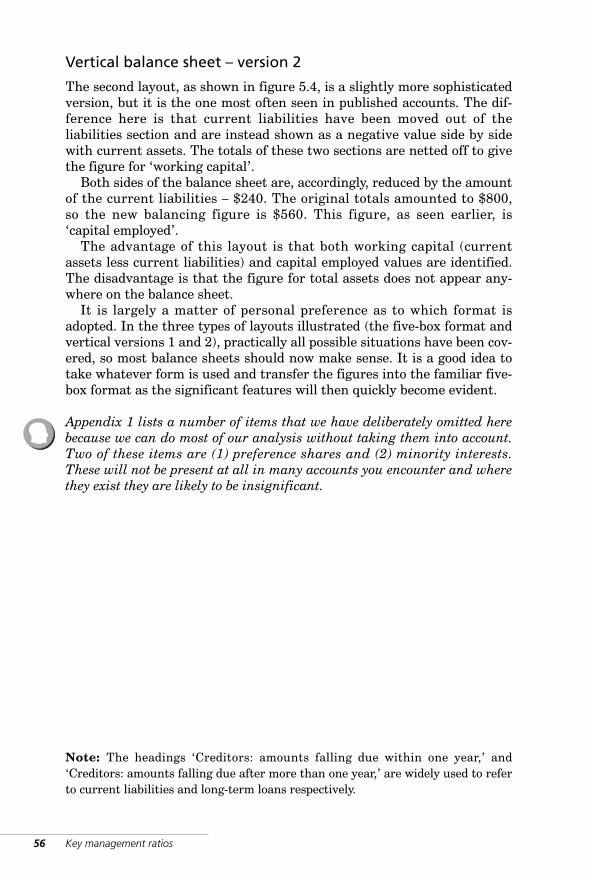
56 Key management ratios
Vertical balance sheet – version 2
The second layout, as shown in figure 5.4, is a slightly more sophisticatedversion, but it is the one most often seen in published accounts. The dif-ference here is that current liabilities have been moved out of theliabilities section and are instead shown as a negative value side by sidewith current assets. The totals of these two sections are netted off to givethe figure for ‘working capital’.
Both sides of the balance sheet are, accordingly, reduced by the amountof the current liabilities – $240. The original totals amounted to $800,so the new balancing figure is $560. This figure, as seen earlier, is‘capital employed’.
The advantage of this layout is that both working capital (currentassets less current liabilities) and capital employed values are identified.The disadvantage is that the figure for total assets does not appear any-where on the balance sheet.
It is largely a matter of personal preference as to which format isadopted. In the three types of layouts illustrated (the five-box format andvertical versions 1 and 2), practically all possible situations have been cov-ered, so most balance sheets should now make sense. It is a good idea totake whatever form is used and transfer the figures into the familiar five-box format as the significant features will then quickly become evident.
Appendix 1 lists a number of items that we have deliberately omitted herebecause we can do most of our analysis without taking them into account.Two of these items are (1) preference shares and (2) minority interests.These will not be present at all in many accounts you encounter and wherethey exist they are likely to be insignificant.
Note: The headings ‘Creditors: amounts falling due within one year,’ and‘Creditors: amounts falling due after more than one year,’ are widely used to referto current liabilities and long-term loans respectively.
WKMR_CH05.QXD 11/24/05 12:18 PM Page 56
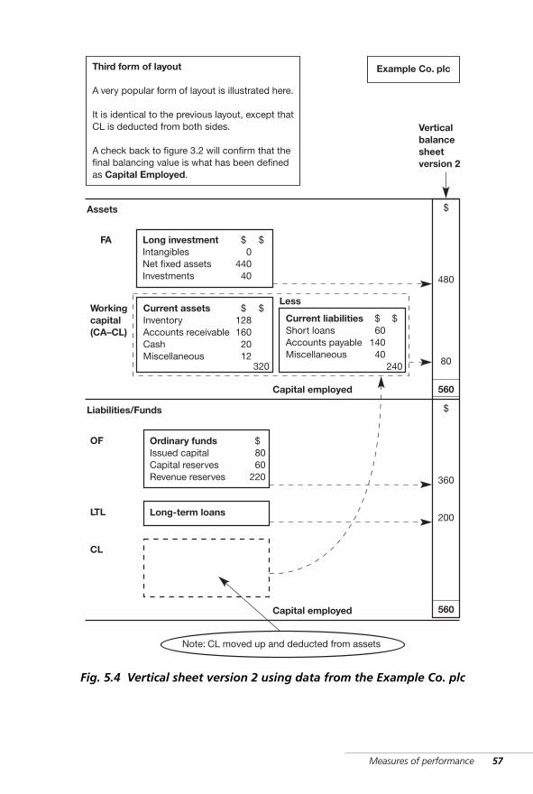
Measures of performance 57
Third form of layout
A very popular form of layout is illustrated here.
It is identical to the previous layout, except thatCL is deducted from both sides.
A check back to figure 3.2 will confirm that thefinal balancing value is what has been definedas Capital Employed.
Long investmentIntangiblesNet fixed assetsInvestments
044040
$
Current assetsInventoryAccounts receivableCashMiscellaneous
$1281602012
Ordinary fundsIssued capitalCapital reservesRevenue reserves
8060
220
$
Long-term loans
Verticalbalancesheetversion 2
$
480
Capital employed
Capital employed
80
560
360
200
560
Assets
OF
Workingcapital(CA–CL)
LTL
CL
Current liabilitiesShort loansAccounts payableMiscellaneous
6014040
$
FA
Less$
$
320 240
$
Liabilities/Funds
Note: CL moved up and deducted from assets
Example Co. plc
$
Fig. 5.4 Vertical sheet version 2 using data from the Example Co. plc
WKMR_CH05.QXD 11/24/05 12:18 PM Page 57

WKMR_CH05.QXD 11/24/05 12:18 PM Page 58
6 OperatingperformanceReturn on investment (ROI)
· Return on equity (ROE)
· Return on total assets (ROTA)
· Standards of operating performance
But the age of chivalry is gone. That ofsophisters, economists, and calculators, hassucceeded; and the glory of Europe isextinguished for ever.EDMUND BURKE (1729–1797)
WKMR_CH06.QXD 11/24/05 12:18 PM Page 59

WKMR_CH06.QXD 11/24/05 12:18 PM Page 60
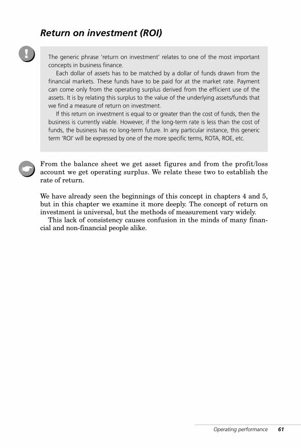
Operating performance 61
Return on investment (ROI)
From the balance sheet we get asset figures and from the profit/lossaccount we get operating surplus. We relate these two to establish therate of return.
We have already seen the beginnings of this concept in chapters 4 and 5,but in this chapter we examine it more deeply. The concept of return oninvestment is universal, but the methods of measurement vary widely.
This lack of consistency causes confusion in the minds of many finan-cial and non-financial people alike.
The generic phrase ‘return on investment’ relates to one of the most importantconcepts in business finance.
Each dollar of assets has to be matched by a dollar of funds drawn from thefinancial markets. These funds have to be paid for at the market rate. Paymentcan come only from the operating surplus derived from the efficient use of theassets. It is by relating this surplus to the value of the underlying assets/funds thatwe find a measure of return on investment.
If this return on investment is equal to or greater than the cost of funds, then thebusiness is currently viable. However, if the long-term rate is less than the cost offunds, the business has no long-term future. In any particular instance, this genericterm ‘ROI’ will be expressed by one of the more specific terms, ROTA, ROE, etc.
!
☛
WKMR_CH06.QXD 11/24/05 12:18 PM Page 61
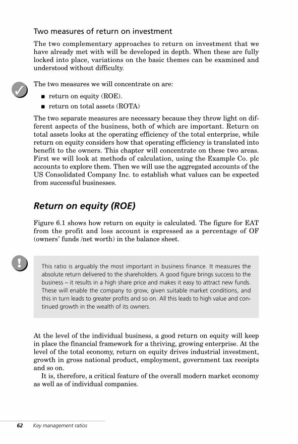
62 Key management ratios
Two measures of return on investment
The two complementary approaches to return on investment that wehave already met with will be developed in depth. When these are fullylocked into place, variations on the basic themes can be examined andunderstood without difficulty.
The two measures we will concentrate on are:
■ return on equity (ROE).■ return on total assets (ROTA)
The two separate measures are necessary because they throw light on dif-ferent aspects of the business, both of which are important. Return ontotal assets looks at the operating efficiency of the total enterprise, whilereturn on equity considers how that operating efficiency is translated intobenefit to the owners. This chapter will concentrate on these two areas.First we will look at methods of calculation, using the Example Co. plcaccounts to explore them. Then we will use the aggregated accounts of theUS Consolidated Company Inc. to establish what values can be expectedfrom successful businesses.
Return on equity (ROE)
Figure 6.1 shows how return on equity is calculated. The figure for EATfrom the profit and loss account is expressed as a percentage of OF(owners’ funds /net worth) in the balance sheet.
At the level of the individual business, a good return on equity will keepin place the financial framework for a thriving, growing enterprise. At thelevel of the total economy, return on equity drives industrial investment,growth in gross national product, employment, government tax receiptsand so on.
It is, therefore, a critical feature of the overall modern market economyas well as of individual companies.
✓
This ratio is arguably the most important in business finance. It measures theabsolute return delivered to the shareholders. A good figure brings success to thebusiness – it results in a high share price and makes it easy to attract new funds.These will enable the company to grow, given suitable market conditions, andthis in turn leads to greater profits and so on. All this leads to high value and con-tinued growth in the wealth of its owners.
!
WKMR_CH06.QXD 11/24/05 12:18 PM Page 62
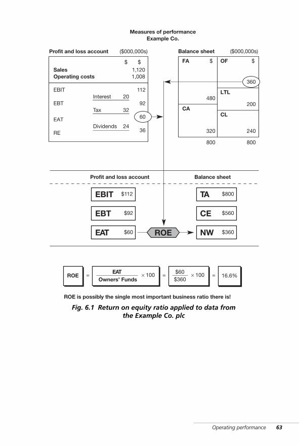
Operating performance 63
EATOwners’ Funds
$60$360
16.6%× 100 × 100= = =ROE
ROE is possibly the single most important business ratio there is!
Profit and loss account Balance sheet
EBIT
EBT
EAT
TA
CE
NWROE
$112
$92
$60
$800
$560
$360
SalesOperating costs
Profit and loss account
1,1201,008
$
800800
FA
CA
OF
LTL
CL
240320
200480
Balance sheet ($000,000s)
$$$
($000,000s)
Measures of performanceExample Co.
EBIT
EBT
EAT
RE
Interest
Tax
Dividends
20
32
24
360
112
92
60
36
Fig. 6.1 Return on equity ratio applied to data fromthe Example Co. plc
WKMR_CH06.QXD 11/24/05 12:18 PM Page 63
64 Key management ratios
Return on total assets (ROTA)
Return on total assets provides the foundation necessary for a company todeliver a good return on equity. A company without a good ROTA finds italmost impossibe to generate a satisfactory ROE. Figure 6.2 shows howROTA is calculated, i.e. EBIT/TA.
EBIT is the amount remaining when total operating cost is deductedfrom total revenue, but before either interest or tax have been paid. Totaloperating cost includes direct factory cost, plus administration, sellingand distribution overheads.
This operating profit figure is set against the total assets figure in thebalance sheet. The percentage relationship between the two values givesthe rate of return being earned by the total assets. Therefore this ratiomeasures how well management uses all the assets in the business to gen-erate an operating surplus.
Some practitioners contend that the figure taken from the balance sheetshould include the long-term funds and only those short-term funds forwhich a charge is made, i.e. STL (short-term loans). Their position is thatassets funded by ‘free’ creditors should not be included in the rate of returncalculation. There is considerable merit in this argument, but a counterargument is that the rate of return issue is separate from the funding issueand that assets should produce a return irrespective of the method of fund-ing. For example, some companies choose to fund by suppliers’ credit,others from a bank loan. The author’s view is that, for most companies, thebalance of advantage lies with the latter school of thought.
Whichever method of calculation is adopted, return on total assets usesthe three main operating variables of the business:
■ total revenue■ total cost■ assets utilized (some definition of).
It is therefore the most comprehensive measure of total management per-formance available to us.
✓
WKMR_CH06.QXD 11/24/05 12:18 PM Page 64
Operating performance 65
EBITTotal Assets
112800
14.0%× 100 × 100= = =
ROTA is the most important driver of ROE!
Profit and loss account Balance sheet
EBIT
EBT
EAT
TA
CE
NW
ROTA$112
$92
$60
$800
$560
$360
SalesOperating costs
Profit and loss account
1,1201,008
$
20
32
24
800800
FA
CA
OF
LTL
CL
240320
200480
Balance sheet ($000,000s)
$$$
($000,000s)
Measure of performanceExample Co.
EBIT
EBT
EAT
RE
Interest
Tax
Dividends
360
ROTA
112
92
60
36
Fig. 6.2 Return on total assets ratio applied to data fromthe Example Co. plc
WKMR_CH06.QXD 11/24/05 12:18 PM Page 65
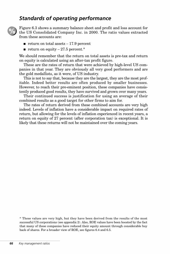
66 Key management ratios
Standards of operating performance
Figure 6.3 shows a summary balance sheet and profit and loss account forthe US Consolidated Company Inc. in 2000. The ratio values extractedfrom these accounts are:
■ return on total assets – 17.9 percent■ return on equity – 27.5 percent.*
We should remember that the return on total assets is pre-tax and returnon equity is calculated using an after-tax profit figure.
These are the rates of return that were achieved by high-level US com-panies in that year. They are obviously all very good performers and arethe gold medallists, as it were, of US industry.
This is not to say that, because they are the largest, they are the most prof-itable. Indeed better results are often produced by smaller businesses.However, to reach their pre-eminent position, these companies have consis-tently produced good results, they have survived and grown over many years.
Their continued success is justification for using an average of theircombined results as a good target for other firms to aim for.
The rates of return derived from these combined accounts are very highindeed. Levels of inflation have a considerable impact on required rates ofreturn, but allowing for the levels of inflation experienced in recent years, areturn on equity of 27 percent (after corporation tax) is exceptional. It islikely that these returns will not be maintained over the coming years.
%
* These values are very high, but they have been derived from the results of the mostsuccessful US corporations (see appendix 2). Also, ROE values have been boosted by the factthat many of these companies have reduced their equity amount through considerable buyback of shares. For a broader view of ROE, see figures 6.4 and 6.5.
WKMR_CH06.QXD 11/24/05 12:18 PM Page 66
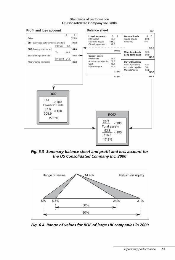
Operating performance 67
EBIT
Total assets
17.9%
× 100
ROTA
92.8516.8
× 100
EAT
Owners’ funds
27.5%
× 100
ROE
57.6208.9
× 100
Profit and loss account Balance sheet
Standards of performanceUS Consolidated Company Inc. 2000
Long investmentIntangiblesNet fixed assetsOther long assets
Current assetsInventoriesAccounts receivableCashMiscellaneous
Owners’ fundsIssued capitalReserves
Misc. long fundsLong-term loans
Current liabilitiesShort-term loansAccounts payableMiscellaneous
Sales 22.8186.1
$
208.9
$
143.2
42.456.166.2
164.7
516.8
66.2185.049.0
$
300.2
$
86.668.240.421.4
216.6
516.8
725.9$
EBIT (Earnings before interest and tax)
EBT (Earnings before tax)
EAT (Earnings after tax)
RE (Retained earnings)
Interest
Tax
Dividend
8.5
26.7
21.6
92.8
84.3
57.6
36.0
$bn
$
52.390.9
Fig. 6.3 Summary balance sheet and profit and loss account forthe US Consolidated Company Inc. 2000
5% 8.5% 24% 31%50%
80%
14.4%Range of values Return on equity
Fig. 6.4 Range of values for ROE of large UK companies in 2000
WKMR_CH06.QXD 11/24/05 12:18 PM Page 67
68 Key management ratios
Return on equity – geographic and sectoral analysis
We have described return on equity as being, probably, the single most impor-tant financial ratio we have. It is the great driver of company value. Thereforeit is important to know what is happening in the world in terms of this ratio.
From very profitable companies in the US and the UK we get very highvalues of approximately 25 percent. Figure 6.4 reflects results of researchon simply the largest UK companies in 2000.
The results of current research into approximately 200 worldwide compa-nies are shown in figure 6.5.
In Chart (a), we see that there is a wide spread between the US and UKon the one hand and the EU and Japan on the other. In the former coun-tries, we see returns in the high 20s; in the latter we see rates just aboveand below 10 percent.
Some of these variations can be explained by the differences in methods ofaccounting. For instance, in an environment that has experienced heavytakeover activity, followed by high goodwill write-offs, equity values in thebalance sheet no longer give us a true value for shareholders’ investment,and ROE values would be overstated accordingly. It is the author’s opinionthat an ROE of 15 percent is a very satisfactory return.
Across the industrial sectors there is no regular pattern between coun-tries. The low overall return for Japan is consistent across all sectors. Thefood sector is the worst offender. It yields only 5 percent. It has shown adramatic decline over the previous four years, indicating perhaps that thestrong yen has caused the greatest damage here.
Outstanding at the other end of the scale are the very high returnsbeing delivered by the US food sector. Included in this category are world-famous names such as Kellogg, Campbell’s Soup, Hershey Foods, etc.These companies with powerful brand identification deliver extraordinarylevels of profit.
It is interesting that this is the sector where companies have bought back a consider-able amount of their own shares, a fact that suggests that they have difficulty infinding outlets for their enormous cash flow that will not dilute their very high returns.
!
%
%
WKMR_CH06.QXD 11/24/05 12:18 PM Page 68
Operating performance 69
20.0%
15.0%
10.0%
5.0%
0.0%
EU: ROE by sector
(d)
Mach Food Drug Retail All
20.0%
15.0%
10.0%
5.0%
0.0%
Japan: ROE by sector
(e)
Mach Food Drug Retail All
30.0%
15.0%
10.0%
5.0%
0.0%US
ROE by country
(a)UK EU JP All
25.0%
20.0%
50.0%
40.0%
30.0%
20.0%
10.0%
0.0%
US: ROE by sector
(b)
Mach Food Drug Retail All
50.0%
40.0%
30.0%
20.0%
10.0%
0.0%
UK: ROE by sector
(c)
Mach Food Drug Retail All
Fig. 6.5 Return on equity by country and by sector
WKMR_CH06.QXD 11/24/05 12:18 PM Page 69
70 Key management ratios
Return on total assets – geographical and sectoral analysis
When we look at standard values for ROTA and ROE, the effects of lever-age are clearly seen. Even though ROTA is a pre-tax measure itconsistently comes out 3 percent to 6 percent less than after-tax ROEvalues. In the US and UK economies we find results of 14 percent to 16percent. Figure 6.6 shows that 50 percent of companies clustered within arange of 8.5 percent plus or minus 3 percent.
However figure 6.7 shows that these values again far exceed the rest of theworld. Japanese companies and EU companies produce about 7 percent.
The drug sector in the US again shows outstanding results. All sectorsin Japan except drugs produce results we would consider to be very low.
* The links between these two ratios are discussed in chapter 13.
A company in the western world would currently need to set its sights on attain-ing a value of 8 percent to 12 percent as a ‘return to total assets’ ratio. This isquite a difficult value to achieve and it may have to fall in the coming years.
!
We know that this is the second great performance measure and its importancecannot be over-stated. It is:
■ the greatest single driver of return on equity*
■ the prime measure of operating efficiency
■ the ratio over which operations management has most control.
Figures 6.6 and 6.7 will help to set targets for good performance.
!
%
WKMR_CH06.QXD 11/24/05 12:18 PM Page 70
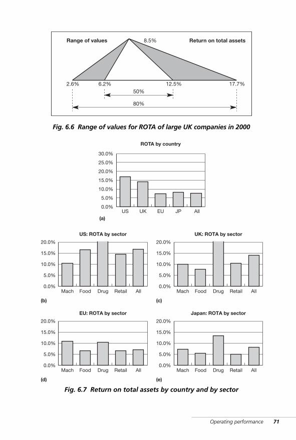
Operating performance 71
20.0%
15.0%
10.0%
5.0%
0.0%
EU: ROTA by sector
(d)
Mach Food Drug Retail All
20.0%
15.0%
10.0%
5.0%
0.0%
Japan: ROTA by sector
(e)
Mach Food Drug Retail All
30.0%
15.0%
10.0%
5.0%
0.0%US
ROTA by country
(a)UK EU JP All
25.0%
20.0%
20.0%
15.0%
10.0%
5.0%
0.0%
US: ROTA by sector
(b)
Mach Food Drug Retail All
20.0%
15.0%
10.0%
5.0%
0.0%
UK: ROTA by sector
(c)
Mach Food Drug Retail All
Fig. 6.7 Return on total assets by country and by sector
2.6% 6.2% 12.5% 17.7%50%
80%
8.5%Range of values Return on total assets
Fig. 6.6 Range of values for ROTA of large UK companies in 2000
WKMR_CH06.QXD 11/24/05 12:18 PM Page 71
72 Key management ratios
The components of return on total assets
Return on total assets is a key tool in directing management’s day-to-dayactivities. It provides a benchmark against which all operations can bemeasured. However as a single figure it simply provides a target. To beuseful in decision making it must first be broken down into its componentparts. This will now be done in two stages. First the main ratio is dividedinto two subsidiary ratios (see figure 6.8), then each of these is furtherdivided into its detailed constituents.
In Stage 1 the two prime subsidiary ratios are identified:
■ margin on sales percentage■ sales to total assets ratio (asset turn).
ROTA is calculated by the fraction : EBIT/TA. We introduce the figure for‘Sales’ and link it to each variable to give us two fractions instead of one.We get the ratios (a)EBIT/sales (profit margin) and (b)sales/TA (assetturn). It is simple mathematics to show that the product of these willalways combine to the value of ROTA. This first split is so important thatwe will take the risk of over-emphasizing it here. The formula is:
Profit AssetROTA = ×
Margin Turn
EBIT EBIT Sales*= ×
TA Sales* TA
* Note that ‘Sales’ cancel out above and below the line.
$14 $14 $200= ×
$100 $200 $100
14% = 7% × 2 times
We have now derived two most important ratios, ‘profit margin’ and‘asset turn’. The former identifies profit as a percentage of sales and isoften described as the net profit margin. It is a well-known measure andalmost universally used in the monitoring of a company’s profitability.
The latter ratio looks at the total sales achieved by the company inrelation to its total assets, a measure that is less often emphasized in theassessment of company performance. However its contribution to ROTAis just as powerful and important as the profit margin.
%
☛
WKMR_CH06.QXD 11/24/05 12:18 PM Page 72
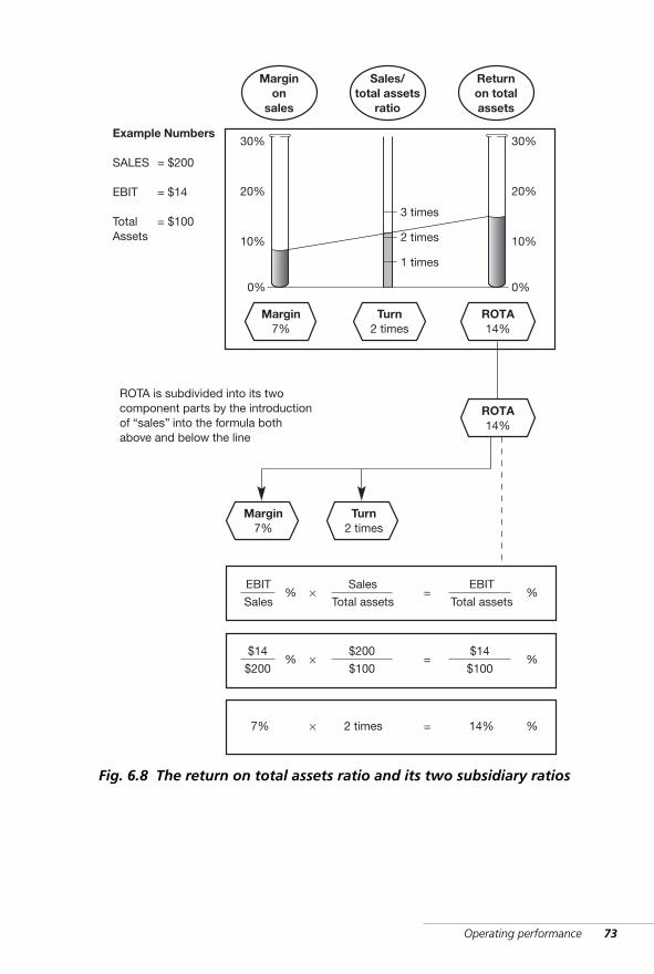
Operating performance 73
Example Numbers
SALES
EBIT
TotalAssets
0%
30%
3 times
2 times
1 times
Margin7%
Turn2 times
ROTA14%
20%
10%
Marginon
sales
Sales/total assets
ratio
Returnon totalassets
0%
30%
20%
10%
= $200
= $14
= $100
Margin7%
Turn2 times
EBIT
Sales% ×
Sales
Total assets= %
EBIT
Total assets
$14
$200% ×
$200
$100= %
$14
$100
7% × 2 times = %14%
ROTA is subdivided into its twocomponent parts by the introductionof “sales” into the formula bothabove and below the line
ROTA14%
Fig. 6.8 The return on total assets ratio and its two subsidiary ratios
WKMR_CH06.QXD 11/24/05 12:18 PM Page 73
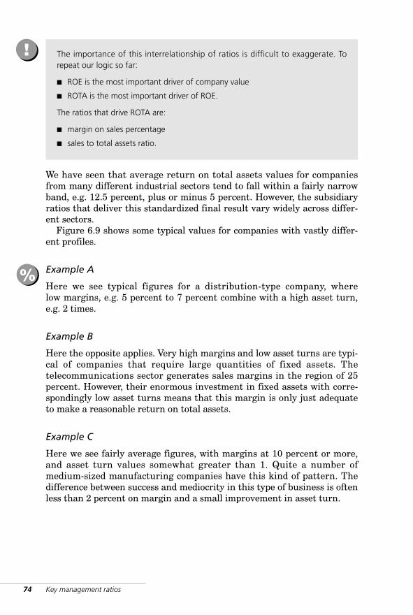
74 Key management ratios
We have seen that average return on total assets values for companiesfrom many different industrial sectors tend to fall within a fairly narrowband, e.g. 12.5 percent, plus or minus 5 percent. However, the subsidiaryratios that deliver this standardized final result vary widely across differ-ent sectors.
Figure 6.9 shows some typical values for companies with vastly differ-ent profiles.
Example A
Here we see typical figures for a distribution-type company, wherelow margins, e.g. 5 percent to 7 percent combine with a high asset turn,e.g. 2 times.
Example B
Here the opposite applies. Very high margins and low asset turns are typi-cal of companies that require large quantities of fixed assets. Thetelecommunications sector generates sales margins in the region of 25percent. However, their enormous investment in fixed assets with corre-spondingly low asset turns means that this margin is only just adequateto make a reasonable return on total assets.
Example C
Here we see fairly average figures, with margins at 10 percent or more,and asset turn values somewhat greater than 1. Quite a number ofmedium-sized manufacturing companies have this kind of pattern. Thedifference between success and mediocrity in this type of business is oftenless than 2 percent on margin and a small improvement in asset turn.
The importance of this interrelationship of ratios is difficult to exaggerate. Torepeat our logic so far:
■ ROE is the most important driver of company value
■ ROTA is the most important driver of ROE.
The ratios that drive ROTA are:
■ margin on sales percentage
■ sales to total assets ratio.
!
%
WKMR_CH06.QXD 11/24/05 12:18 PM Page 74
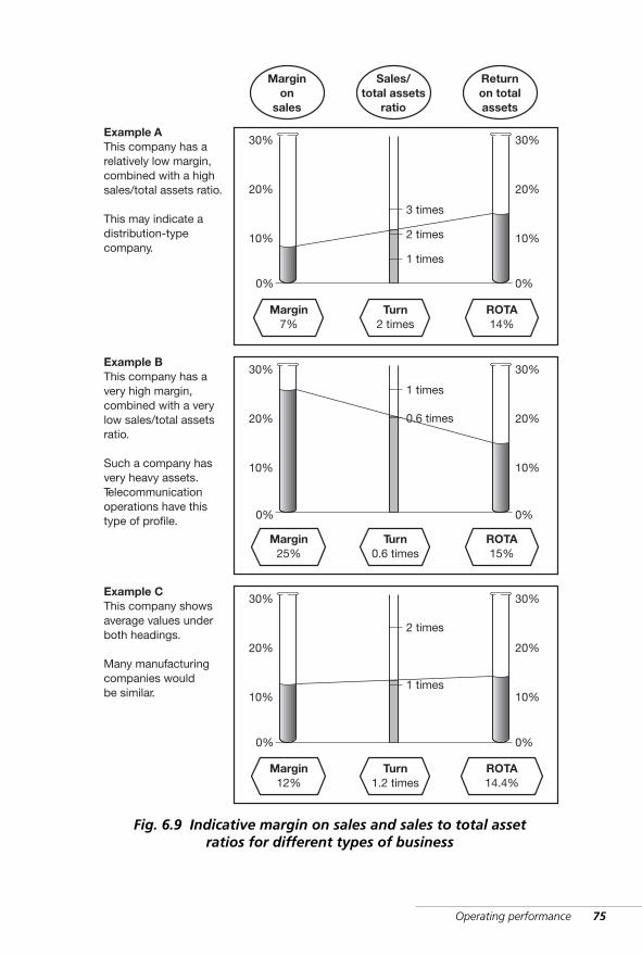
Operating performance 75
Example AThis company has arelatively low margin,combined with a highsales/total assets ratio.
This may indicate adistribution-typecompany.
0%
30%
3 times
2 times
1 times
Margin7%
Turn2 times
ROTA14%
20%
10%
Example BThis company has avery high margin,combined with a verylow sales/total assetsratio.
Such a company hasvery heavy assets.Telecommunicationoperations have thistype of profile. 0%
30%
0.6 times
1 times
Margin25%
Turn0.6 times
ROTA15%
20%
10%
Example CThis company showsaverage values underboth headings.
Many manufacturingcompanies wouldbe similar.
0%
30%
2 times
1 times
Margin12%
Turn1.2 times
ROTA14.4%
20%
10%
Marginon
sales
Sales/total assets
ratio
Returnon totalassets
0%
30%
20%
10%
0%
30%
20%
10%
0%
30%
20%
10%
Fig. 6.9 Indicative margin on sales and sales to total assetratios for different types of business
WKMR_CH06.QXD 11/24/05 12:18 PM Page 75
76 Key management ratios
‘Margin’ and ‘Sales to Total Assets’ standards
Figure 6.10 illustrates the calculations and results for the US ConsolidatedCompany Inc. An average sales margin of 12.8 percent is delivered 1.4times to produce a ‘return on total assets’ value of 17.9 percent.
A comparison by country (see figure 6.11) shows a strong similaritybetween companies in the US and the UK. In the US a slightly lowermargin is accompanied by a somewhat higher ‘sales to total assets’.However the size of the sample would not allow us to give great statisticalsignificance to these variations.
Companies in the EU seem to operate on lower margins and their assetutilization is also low. Companies in Japan operate on low margins butappear to have a somewhat better assets utilization. This latest finding runscontrary to popular belief. Much has been written about Japanese achieve-ments in operating with very low inventory levels. While this may be true inspecific industries it does not seem to hold across a wide range of companies.
It rests with the skill of each management team to discover for itself theunique combination of margin and asset turn that will give their companyits own particular, and successful, market niche.
A rule of thumb would be that a margin of approximately 10 percent, combinedwith an asset turn of between 1.3 and 1.5 would be where many western com-panies would find a comfortable and profitable position.
!
☛
WKMR_CH06.QXD 11/24/05 12:18 PM Page 76
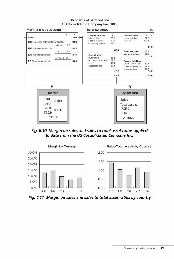
Operating performance 77
30.0%
20.0%
10.0%
0.0%US
Margin by Country
UK EU JP All
2.00
1.50
1.00
0.50
0.00US
Sales/Total assets by Country
UK EU JP All
25.0%
15.0%
5.0%
Fig. 6.11 Margin on sales and sales to total asset ratios by country
EBIT
Sales
12.8%
× 100
Margin
92.8725.9
× 100
Profit and loss account Balance sheet
Standards of performanceUS Consolidated Company Inc. 2000
Long investmentIntangiblesNet fixed assetsOther long assets
Current assetsInventoriesAccounts receivableCashMiscellaneous
Owners’ fundsIssued capitalReserves
Misc. long fundLong-term loan
Current liabilitiesShort-term loansAccounts payableMiscellaneous
Sales 22.8186.1
$
208.9
$
143.2
42.456.166.2
164.7
516.8
66.2185.049.0
$
300.2
$
86.668.240.421.4
216.6
516.8
725.9$
EBIT (Earnings before interest and tax)
EBT (Earnings before tax)
EAT (Earnings after tax)
RE (Retained earnings)
Interest
Tax
Dividend
8.5
26.7
21.6
92.8
84.3
57.6
36.0
$bn
$
52.390.9
Sales
Total assets
1.4 times
Asset turn
725.9516.8
Fig. 6.10 Margin on sales and sales to total asset ratios appliedto data from the US Consolidated Company Inc.
WKMR_CH06.QXD 11/24/05 12:18 PM Page 77
Sector parameters – return on total assets
In figure 6.12, results of research into top UK companies in 1992 are stillused here because they give a dramatic illustration of the interrelation-ship that exists between the two key variables that determine what acompany will achieve in terms of return on total assets.
Chart A shows values for ‘Sales to total assets’ and chart B ‘Margin’values for six industrial sectors ranging from ‘food’ to ‘health care’. Thetwo charts are almost minor images of one another. High sales to assetsratios are generally offset by low margins and vice versa. It is where theminor images do not exactly match where the high and low performersare located.
The values shown in Chart A of figure 6.12 point to a question concern-ing business performance that is absolutely critical. What level ofinvestment is required to support any given level of sales? The results dis-played here help us to understand why some sectors of industry seem tohave a built-in advantage over others.
Chart A shows the high sales to total assets ratios inherent in the foodindustry. While this ratio is high in both retailing and manufacturing sec-tors, it is more pronounced in retailing.
Chemicals and stores both have ‘sales to total asset’ ratios that areapproximately 20 percent above the average, but this advantage is mostlyoffset by their lower margins – particularly in the case of chemicals. Thetwo sectors are still quite good overall.
When we look to the two final sectors, we see a dramatic contrast. Thebrewing value is very low, with a sales to total assets ratio of about 0.6times. It may be more informative to turn this ratio upside down and saythat it requires $1.60 of assets to carry $l.00 of sales. For any given levelof sales, the investment in assets is enormous. In contrast, in the foodretailing sector it takes only $0.45 to support $1.00 of sales. The brew-ing/distilling sector requires almost four times this investment to producethis result.
In the health sector, we note that the ‘sales to total assets’ ratio is alsobelow average but this sector has a margin on sales that compensates byalmost 200 percent for these somewhat high assets. The high margins inbrewing are still not sufficient to pay for the very high investment inassets in this sector.
78 Key management ratios
%
WKMR_CH06.QXD 11/24/05 12:18 PM Page 78
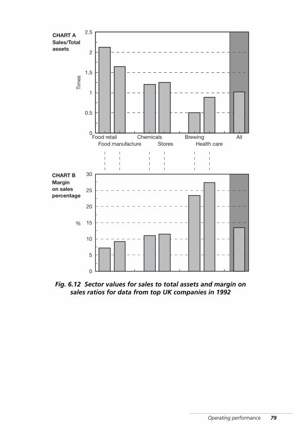
Operating performance 79
CHART A
0Food retail
Food manufactureChemicals
StoresBrewing
Health careAll
Sales/Totalassets
Tim
es
CHART BMarginon salespercentage
0.5
1
1.5
2
2.5
0
%
5
10
15
20
25
30
Fig. 6.12 Sector values for sales to total assets and margin onsales ratios for data from top UK companies in 1992
WKMR_CH06.QXD 11/24/05 12:18 PM Page 79

WKMR_CH06.QXD 11/24/05 12:18 PM Page 80
7 Performance driversOperating performance
· Operating profit model
Everything, then, must be assessed in money;for this enables men always to exchange theirservices, and so makes society possible.ARISTOTLE (384–322 BC)
WKMR_CH07.QXD 11/24/05 12:19 PM Page 81
82 Key management ratios
Operating performance
The two prime ratios that drive return on total assets have been identified:
■ margin on sales percentage■ sales to total assets ratio
and these are laid out again for the Example Co. plc in figure 7.1.
It is on these two drivers that managers must concentrate in order toimprove performance. However, these ratios cannot be operated on directly.Each is dependent on a whole series of detailed results from widely sepa-rated parts of the operation. These in turn can be expressed in ratio formand all that managers need is a system that will enable them to identify andquantify these subsidiary values so that they can:
■ set the target value for each ratio that, if achieved, will deliver therequired overall performance level
■ delegate the achievement of these targets to specific individuals.
The system outlined in the following pages achieves this end. It will beseen that it incorporates all the main elements in both the profit and lossaccount and balance sheet. Each of the elements is a performance driverand must be managed accordingly.
Drivers of margin on sales
If the margin were 10 percent, the total cost would be 90 percent. Themargin can be improved only if this 90 percent can be reduced. To reducethe figure, we must know its component parts. So, the next stage is iden-tify the separate cost elements and see what percentage each of the maincost elements bears to sales (see figure 7.2).
Drivers of the sales to total assets ratio
This ratio is also broken down into its component parts. We identify themain groups of assets straight from the balance sheet and we thenexpress the ratio between each group and the sales figure as shownin figure 7.3.
✓
At its simplest, we can say that the margin is what is left when the total operat-ing cost is deducted.
!
WKMR_CH07.QXD 11/24/05 12:19 PM Page 82
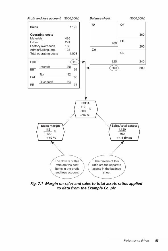
Performance drivers 83
Sales
Operating costsMaterialsLaborFactory overheadsAdmin/Selling, etc.Total operating costs
Profit and loss account
1,120
1,008
EBIT
EBT
EAT
RE
Interest
Tax
Dividends
20
32
24
112
92
60
36
800 800
FA
CA
OF
LTL
CL
240320
200
360
480
Balance sheet ($000,000s)($000,000s)
ROTA112800
14 %
%
=
Sales/total assets1,1208001.4 times=
Sales margin112
1,12010 %
%
=
426291168123
The drivers of thisratio are the costitems in the profitand loss account
The drivers of thisratio are the separateassets in the balance
sheet
Fig. 7.1 Margin on sales and sales to total assets ratios appliedto data from the Example Co. plc
WKMR_CH07.QXD 11/24/05 12:19 PM Page 83
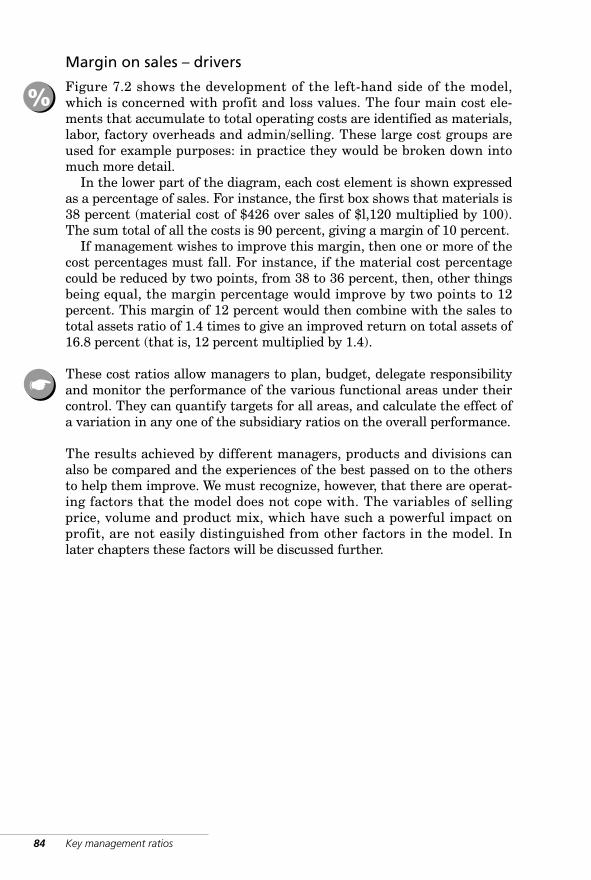
84 Key management ratios
☛
Margin on sales – drivers
Figure 7.2 shows the development of the left-hand side of the model,which is concerned with profit and loss values. The four main cost ele-ments that accumulate to total operating costs are identified as materials,labor, factory overheads and admin/selling. These large cost groups areused for example purposes: in practice they would be broken down intomuch more detail.
In the lower part of the diagram, each cost element is shown expressedas a percentage of sales. For instance, the first box shows that materials is38 percent (material cost of $426 over sales of $l,120 multiplied by 100).The sum total of all the costs is 90 percent, giving a margin of 10 percent.
If management wishes to improve this margin, then one or more of thecost percentages must fall. For instance, if the material cost percentagecould be reduced by two points, from 38 to 36 percent, then, other thingsbeing equal, the margin percentage would improve by two points to 12percent. This margin of 12 percent would then combine with the sales tototal assets ratio of 1.4 times to give an improved return on total assets of16.8 percent (that is, 12 percent multiplied by 1.4).
These cost ratios allow managers to plan, budget, delegate responsibilityand monitor the performance of the various functional areas under theircontrol. They can quantify targets for all areas, and calculate the effect ofa variation in any one of the subsidiary ratios on the overall performance.
The results achieved by different managers, products and divisions canalso be compared and the experiences of the best passed on to the othersto help them improve. We must recognize, however, that there are operat-ing factors that the model does not cope with. The variables of sellingprice, volume and product mix, which have such a powerful impact onprofit, are not easily distinguished from other factors in the model. Inlater chapters these factors will be discussed further.
%
WKMR_CH07.QXD 11/24/05 12:19 PM Page 84
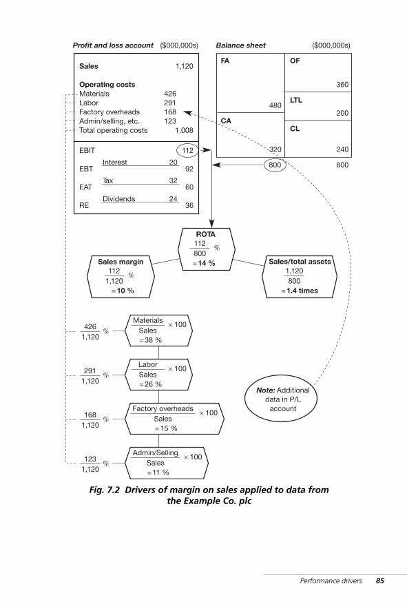
Performance drivers 85
MaterialsSales
38 %
× 100
=
4261,120
%
LaborSales
26 %
× 100
=
2911,120
%
Factory overheadsSales
15 %
× 100
=
1681,120
%
Admin/SellingSales
11 %
× 100
=
1231,120
%
Note: Additionaldata in P/L
account
Sales
Operating costsMaterialsLaborFactory overheadsAdmin/selling, etc.Total operating costs
Profit and loss account
1,120
1,008
EBIT
EBT
EAT
RE
Interest
Tax
Dividends
20
32
24
112
92
60
36
800 800
FA
CA
OF
LTL
CL
240320
200
360
480
Balance sheet ($000,000s)($000,000s)
ROTA112800
14 %
%
= Sales/total assets1,1208001.4 times=
Sales margin112
1,12010 %
%
=
426291168123
Fig. 7.2 Drivers of margin on sales applied to data fromthe Example Co. plc
WKMR_CH07.QXD 11/24/05 12:19 PM Page 85
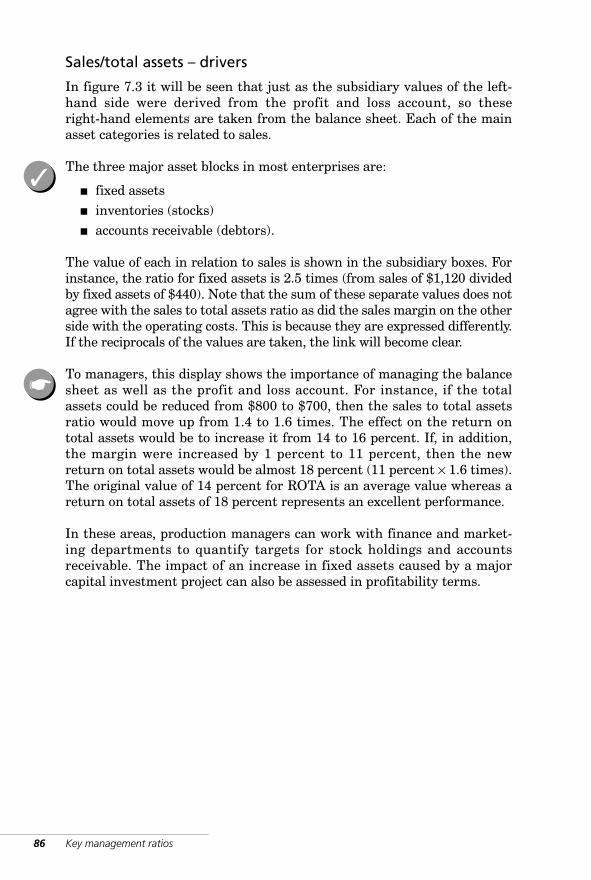
86 Key management ratios
✓
☛
Sales/total assets – drivers
In figure 7.3 it will be seen that just as the subsidiary values of the left-hand side were derived from the profit and loss account, so theseright-hand elements are taken from the balance sheet. Each of the mainasset categories is related to sales.
The three major asset blocks in most enterprises are:
■ fixed assets■ inventories (stocks) ■ accounts receivable (debtors).
The value of each in relation to sales is shown in the subsidiary boxes. Forinstance, the ratio for fixed assets is 2.5 times (from sales of $1,120 dividedby fixed assets of $440). Note that the sum of these separate values does notagree with the sales to total assets ratio as did the sales margin on the otherside with the operating costs. This is because they are expressed differently.If the reciprocals of the values are taken, the link will become clear.
To managers, this display shows the importance of managing the balancesheet as well as the profit and loss account. For instance, if the totalassets could be reduced from $800 to $700, then the sales to total assetsratio would move up from 1.4 to 1.6 times. The effect on the return ontotal assets would be to increase it from 14 to 16 percent. If, in addition,the margin were increased by 1 percent to 11 percent, then the newreturn on total assets would be almost 18 percent (11 percent × 1.6 times).The original value of 14 percent for ROTA is an average value whereas areturn on total assets of 18 percent represents an excellent performance.
In these areas, production managers can work with finance and market-ing departments to quantify targets for stock holdings and accountsreceivable. The impact of an increase in fixed assets caused by a majorcapital investment project can also be assessed in profitability terms.
WKMR_CH07.QXD 11/24/05 12:19 PM Page 86
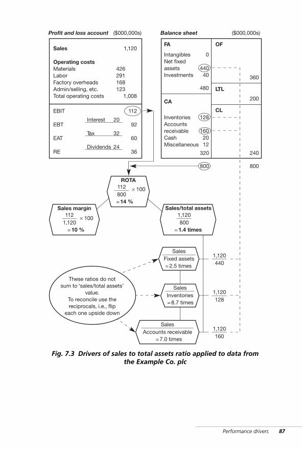
Performance drivers 87
IntangiblesNet fixedassetsInvestments
InventoriesAccountsreceivableCashMiscellaneous
SalesFixed assets
2.5 times=
1,120440
SalesInventories
8.7 times=
1,120128
SalesAccounts receivable
7.0 times=
1,120160
0
44040
128
1602012
320
Sales
Operating costsMaterialsLaborFactory overheadsAdmin/selling, etc.Total operating costs
Profit and loss account
1,120
1,008
EBIT
EBT
EAT
RE
Interest
Tax
Dividends
20
32
24
112
92
60
36
800 800
FA
CA
OF
LTL
CL
240
200
360
480
Balance sheet ($000,000s)($000,000s)
ROTA112800
14 %=Sales/total assets
1,1208001.4 times=
Sales margin112
1,12010 %
× 100
=
426291168123
× 100
These ratios do notsum to ‘sales/total assets’
value.To reconcile use thereciprocals, i.e., flip
each one upside down
Fig. 7.3 Drivers of sales to total assets ratio applied to data fromthe Example Co. plc
WKMR_CH07.QXD 11/24/05 12:19 PM Page 87
88 Key management ratios
Operating profit model
The complete model is shown in figure 7.4. It gives a very powerfulinsight into the drivers of good performance. It enables managers andfunctions to work better together as a team. It helps with the definition ofresponsibilities, delegation of authority and target setting. It provides apowerful framework for a management information system. However,there are a number of issues the model does not highlight.
First, a business normally deals not just in one product, but in a broadrange. Cost percentages are averages of the cost elements of the individualproducts. For management control, it is not satisfactory to work with aver-ages because favorable movements in one product will mask adversemovements in another (these issues are dealt with further in chapter 15).
Second, a cost percentage, such as materials, can vary for two totallydifferent reasons:
■ a change in the absolute material cost per unit■ a change in the unit selling price of the product.
The model, however, cannot distinguish between these two causes,despite the fact that one of the most effective ways to reduce the cost per-centages is a price increase.
Third, the model does not cope very well with changes in volume,which can be one of the most powerful ways open to a company toimprove performance. A volume increase will certainly be picked up bythe sales to total assets ratio – a 10 percent improvement in volume wouldmove this ratio up from 1.4 to 1.54 times – but, because of fixed costs, thevolume change is very likely to have an effect on the sales margin too(this subject is also dealt with in chapter 15).
Fourth, the perceptive reader will have noted that this ratio is depend-ent on the valuation of the assets in the balance sheet. Difficulties canarise when we compare different businesses or divisions because of theage of plant, different depreciation policies and so on.
WKMR_CH07.QXD 11/24/05 12:19 PM Page 88

Performance drivers 89
IntangiblesNet fixedassetsInvestments
InventoryAccountsreceivableCashMiscellaneous
SalesFixed assets
2.5 times=
1,120440
SalesInventory8.7 times=
1,120128
SalesAccounts receivable
7.0 times=
1,120160
0
44040
128
1602012
320
Sales
Operating costsMaterialsLaborFactory overheadsAdmin/selling, etc.Total operating costs
Profit and loss account
1,120
1,008
EBIT
EBT
EAT
RE
Interest
Tax
Ordinary dividends
20
32
24
112
92
60
36
800 800
FA
CA
OF
LTL
CL
240
200
360
480
Balance sheet ($000,000s)($000,000s)
ROTA112800
14 %Sales/total assets
1,1208001.4 times=
Sales margin112
1,12010 %
× 100
=
426291168123
× 100
MaterialsSales
38 %
× 100
=
4261,120
LaborSales
26 %
× 100
=
2911,120
Factory overheadsSales
15 %
× 100
=
1681,120
Admin/SellingSales
11 %× 100
=
1231,120
× 100
× 100
× 100
=
Fig. 7.4 Completed operating profit model applied to data fromthe Example Co. plc
WKMR_CH07.QXD 11/24/05 12:19 PM Page 89
90 Key management ratios
Model variations
Many business ratios appear under different names, or are calculateddifferently, and this can cause some confusion. In the set of ratioswe are looking at here, there are two that appear under a number ofdifferent guises.
Sales to accounts receivable
This ratio is commonly expressed in terms of days’ sales and the methodof calculation is shown in figure 7.5. Instead of the formula we have beenusing here of sales over accounts receivable, the alternative is to showaccounts receivable over sales and multiply the result by 365. The answerrepresents the average number of days’ credit customers take beforepaying off their accounts.
This ratio is often referred to as ‘debtor days’ or the ‘collection period’.The concept of the number of days outstanding is easy to understand. Thenumber is very precise, which means that a slippage of even a few days isinstantly identified. Also, figures can be compared with the company’snormal terms of trade and the effectiveness or otherwise of the credit con-trol department can, therefore, be monitored.
Companies will vary their methods of calculation to reflect their ownbusiness circumstances and to provide answers that make sense to themin particular. For instance:
■ VAT may be included in the debtors but not the sales figure and thisdistortion will have to be removed
■ When there is a heavy seasonal variation, the monthly figurescalculated in the normal way may not be very helpful and so thecompany may work, not on an annual sales basis, but on quarterlysales figures that are annualized.
Sales to inventories
This calculation is similar to the one above and is also known as inventorydays. The link of inventories with sales is not so close as that of sales withaccounts receivable. It may, therefore, be linked to purchases or materialusage, whichever gives the most useful guidance.
WKMR_CH07.QXD 11/24/05 12:19 PM Page 90
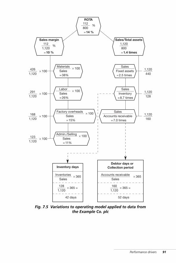
Performance drivers 91
ROTA112800
14 %
%
=
Sales/Total assets1,120800
1.4 times=
SalesFixed assets
2.5 times=
1,120440
Sales margin112
1,12010 %
%
=
SalesInventory8.7 times=
1,120128
SalesAccounts receivable
7.0 times=
1,120160
MaterialsSales
38%
× 100
=
4261,120
× 100
LaborSales
26%
× 100
=
2911,120
× 100
Factory overheadsSales
15%
× 100
=
1681,120
× 100
Admin./SellingSales
11%
× 100
=
1231,120
× 100
InventoriesSales
× 365
Inventory days
1281,120
× 365 =
42 days
Accounts receivableSales
× 365
Debtor days orCollection period
1601,120
× 365 =
52 days
Fig. 7.5 Variations to operating model applied to data fromthe Example Co. plc
WKMR_CH07.QXD 11/24/05 12:19 PM Page 91
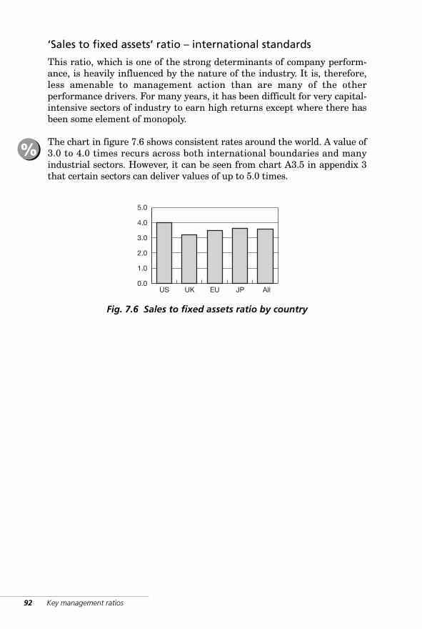
92 Key management ratios
‘Sales to fixed assets’ ratio – international standards
This ratio, which is one of the strong determinants of company perform-ance, is heavily influenced by the nature of the industry. It is, therefore,less amenable to management action than are many of the other performance drivers. For many years, it has been difficult for very capital-intensive sectors of industry to earn high returns except where there hasbeen some element of monopoly.
The chart in figure 7.6 shows consistent rates around the world. A value of3.0 to 4.0 times recurs across both international boundaries and manyindustrial sectors. However, it can be seen from chart A3.5 in appendix 3that certain sectors can deliver values of up to 5.0 times.
%
5.0
3.0
2.0
1.0
0.0US UK EU JP All
4.0
Fig. 7.6 Sales to fixed assets ratio by country
WKMR_CH07.QXD 11/24/05 12:19 PM Page 92
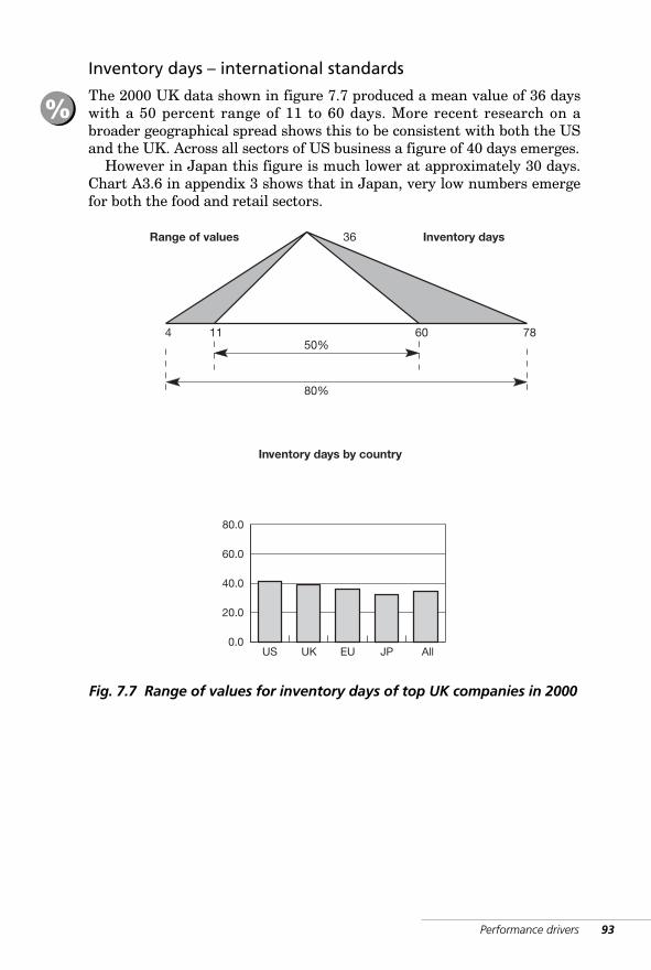
Performance drivers 93
Inventory days – international standards
The 2000 UK data shown in figure 7.7 produced a mean value of 36 dayswith a 50 percent range of 11 to 60 days. More recent research on abroader geographical spread shows this to be consistent with both the USand the UK. Across all sectors of US business a figure of 40 days emerges.
However in Japan this figure is much lower at approximately 30 days.Chart A3.6 in appendix 3 shows that in Japan, very low numbers emergefor both the food and retail sectors.
80.0
60.0
40.0
20.0
0.0US UK EU JP All
Fig. 7.7 Range of values for inventory days of top UK companies in 2000
4 11 60 7850%
80%
36Range of values Inventory days
Inventory days by country
%
WKMR_CH07.QXD 11/24/05 12:19 PM Page 93
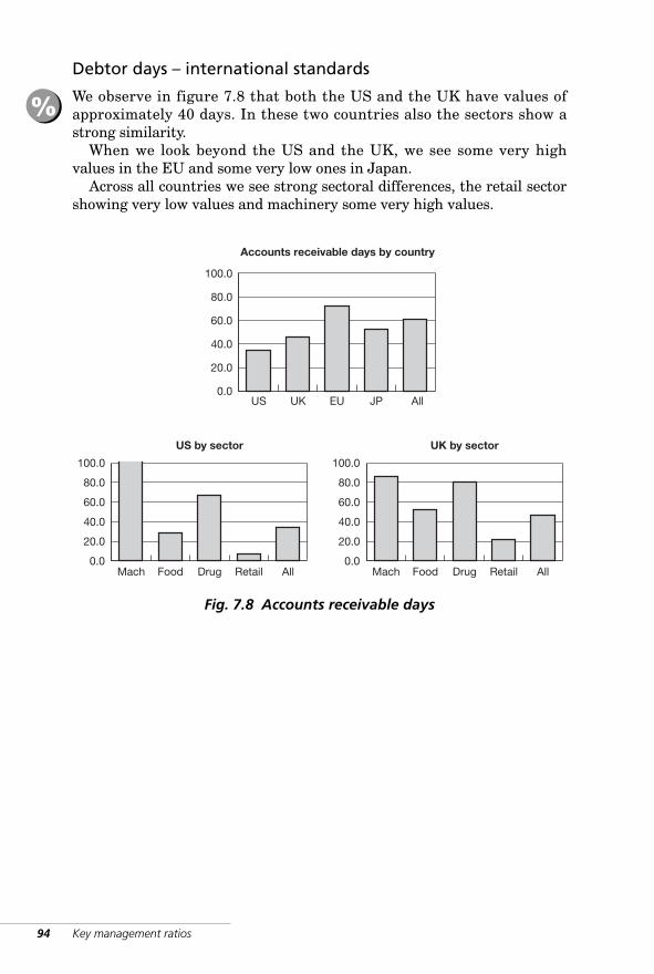
Debtor days – international standards
We observe in figure 7.8 that both the US and the UK have values ofapproximately 40 days. In these two countries also the sectors show astrong similarity.
When we look beyond the US and the UK, we see some very highvalues in the EU and some very low ones in Japan.
Across all countries we see strong sectoral differences, the retail sectorshowing very low values and machinery some very high values.
94 Key management ratios
100.0
60.0
40.0
20.0
0.0US
Accounts receivable days by country
UK EU JP All
80.0
100.0
80.0
40.0
20.0
0.0
US by sector
Mach Food Drug Retail All
100.0
80.0
40.0
20.0
0.0
UK by sector
Mach Food Drug Retail All
60.060.0
Fig. 7.8 Accounts receivable days
%
WKMR_CH07.QXD 11/24/05 12:19 PM Page 94

Part III Corporate liquidity
WKMR_CH08.QXD 11/24/05 12:20 PM Page 95

96 Key management ratios
WKMR_CH08.QXD 11/24/05 12:20 PM Page 96
8 Cash flow cycleCorporate liquidity · The cash cycle
· Measures of liquidity – long and
short analysis
Every branch of knowledge has itsfundamental discovery. In mechanics it isthe wheel, in science fire, in politics the vote.Similarly, in economics, in the wholecommercial side of man’s social existence,money is the essential invention on whichall the rest is based.SIR GEOFFREY CROWTHER (1907–1972)
WKMR_CH08.QXD 11/24/05 12:20 PM Page 97

WKMR_CH08.QXD 11/24/05 12:20 PM Page 98
Cash flow cycle 99
Corporate liquidity
Cash in this case can be a bank account with a positive balance, or it canbe a loan facility that the company has authority to draw down.
When cash runs out, the company’s management has lost the power tomake independent decisions. An outside agency, such as an unpaid credi-tor or a bank whose loan is in default, will decide the fate of the company.
That fate could be bankruptcy, a forced reconstruction, an involuntarytakeover, or the company could be allowed to continue in some alteredform. The reality is that management has lost its authority. It is alsolikely that the owners have lost their entire investment.
One may well ask, ‘How can this happen if profits are good?’ The answeris that it does happen and for reasons that will become clearer later.
Loss of profits is often the immediate cause of the disaster, but as we havesaid, it can happen even when companies are making good profits. Indeed,profitable and rapidly growing small companies very often run out of cash.They then pass out of the hands of the original owner or entrepreneur who isleft with nothing, while others reap the benefits of his enterprise.
This chapter will examine corporate liquidity and the factors that drive it.It will look at how we can measure a company’s liquid health. It will iden-tify the forces that bring benefit or harm to it.
A company must maintain sufficient cash resources to pay all legitimate bills asthey arise. A company that cannot do so has run out of liquidity and is in a veryserious financial condition. Ironically, this is so even if it is currently generatinggood profits.
!
WKMR_CH08.QXD 11/24/05 12:20 PM Page 99
100 Key management ratios
The cash cycle
The flow of cash through an organization is sometimes compared with theflow of blood through the body. When we look at the cash flow diagram infigure 8.1, the reason for this is obvious. Cash is in continuous circulationthrough the ‘arteries’ of the business carrying value to its various‘organs’. If this flow is stopped, or even severely reduced for a time, thenserious consequences result.
This diagram shows part of the total cash cycle, the part that we referto as the working capital cash flow. Central to the system is a cash tank,or reservoir, through which cash flows constantly.
Supporting the cash tank is a supplementary supply, representing unusedshort-term loan facilities. These provide a first line of defense against acash shortage. Day-to-day liquidity consists of these two separate cashreservoirs
The main flow of cash into the reservoir comes from ‘accounts receiv-able’. These are the customers who pay for the goods or services receivedfrom the company.
The main cash out-flows can be identified under two headings:
■ payments to ‘accounts payable’, that is the suppliers of rawmaterials and services
■ payments of staff salaries/wages, and payments of all otheroperating expenses.
We can trace the steps in the cycle. ‘Accounts payable’ supply ‘raw materi-als’. In time these pass through ‘work in process’ into the ‘finished goods’category. During this conversion, cash is absorbed in the form of labor andexpenses and payments to suppliers.
In due course, these ‘finished goods’ are sold. Value passes down theartery into the ‘accounts receivable’ box, from which it flows back into the‘cash’ reservoir to complete the cycle.
It is crucial to the independent survival of the business that this tank does notrun dry.
!
✓
☛
WKMR_CH08.QXD 11/24/05 12:20 PM Page 100
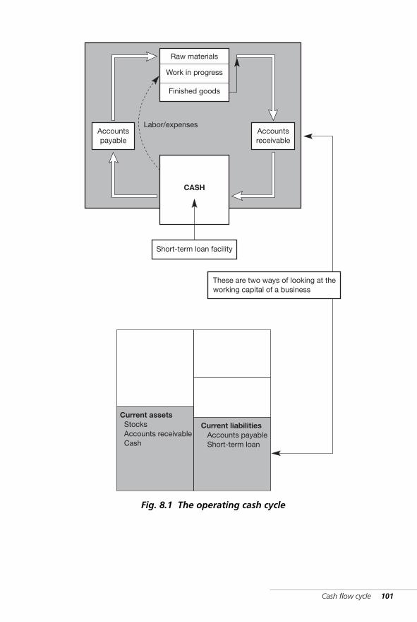
Cash flow cycle 101
Raw materials
Work in progress
Finished goods
Accountspayable
Accountsreceivable
CASH
Short-term loan facility
Current assets Stocks Accounts receivable Cash
Current liabilities Accounts payable Short-term loan
These are two ways of looking at theworking capital of a business
Labor/expenses
Fig. 8.1 The operating cash cycle
WKMR_CH08.QXD 11/24/05 12:20 PM Page 101
102 Key management ratios
Cash flow – the role of profit and depreciation*
In figure 8.2, two further input values are shown that produce an increasein the cash in circulation:
■ profit ■ depreciation.
The input from profit is easy to understand. Normally goods are sold at aprice that exceeds total cost. For instance if goods that cost $100 are soldat a price of $125, the $25 profit will quickly flow into the business in theform of cash.
It is not easy to see why this should be. What is so special about deprecia-tion? The answer is that, for most companies, depreciation is the only costitem in the profit and loss account that does not have a cash out-flowattached to it. While referred to as a source of cash, it is really the avoidanceof a cash out-flow. This point is more fully developed in the following section.
It must be emphasized that, even though depreciation does not have arelated cash out-flow, it is a true cost nevertheless. The relevant cash out-flow has simply taken place at an earlier time. At the time the associatedfixed assets were purchased, the cash cost was not charged against prof-its. It was, instead, charged to the balance sheet. As the asset is used up,an appropriate amount of cost is released into the profit and loss account.This is what depreciation is all about.
It is a little more difficult to understand the input from ‘depreciation’. But depre-ciation is often quoted as a source of funds and we may have seen the definition:
operating cash flow = operating profit + depreciation
?
What figure 8.2 shows is that, with every full cycle, the amount of cash in circula-tion is increased by the profit earned plus the depreciation charged.
!
✓
* Refer to appendix 1 where the technical term EBITDA is explained and discussed.
WKMR_CH08.QXD 11/24/05 12:20 PM Page 102
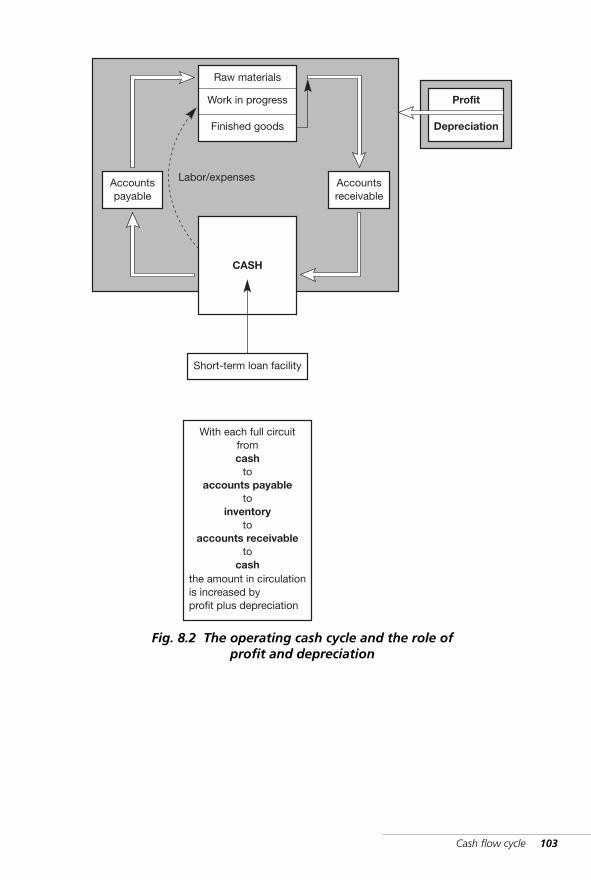
Cash flow cycle 103
Raw materials
Work in progress
Finished goods
Accountspayable
Accountsreceivable
CASH
Short-term loan facility
With each full circuitfromcash
toaccounts payable
toinventory
toaccounts receivable
tocash
the amount in circulationis increased byprofit plus depreciation
Profit
Depreciation
Labor/expenses
Fig. 8.2 The operating cash cycle and the role ofprofit and depreciation
WKMR_CH08.QXD 11/24/05 12:20 PM Page 103
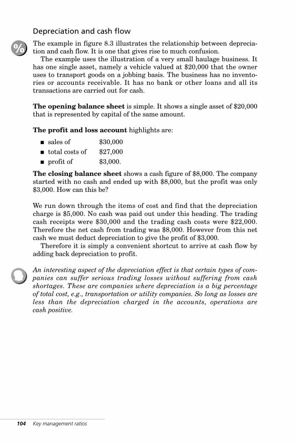
104 Key management ratios
Depreciation and cash flow
The example in figure 8.3 illustrates the relationship between deprecia-tion and cash flow. It is one that gives rise to much confusion.
The example uses the illustration of a very small haulage business. Ithas one single asset, namely a vehicle valued at $20,000 that the owneruses to transport goods on a jobbing basis. The business has no invento-ries or accounts receivable. It has no bank or other loans and all itstransactions are carried out for cash.
The opening balance sheet is simple. It shows a single asset of $20,000that is represented by capital of the same amount.
The profit and loss account highlights are:
■ sales of $30,000 ■ total costs of $27,000 ■ profit of $3,000.
The closing balance sheet shows a cash figure of $8,000. The companystarted with no cash and ended up with $8,000, but the profit was only$3,000. How can this be?
We run down through the items of cost and find that the depreciationcharge is $5,000. No cash was paid out under this heading. The tradingcash receipts were $30,000 and the trading cash costs were $22,000.Therefore the net cash from trading was $8,000. However from this netcash we must deduct depreciation to give the profit of $3,000.
Therefore it is simply a convenient shortcut to arrive at cash flow byadding back depreciation to profit.
An interesting aspect of the depreciation effect is that certain types of com-panies can suffer serious trading losses without suffering from cashshortages. These are companies where depreciation is a big percentageof total cost, e.g., transportation or utility companies. So long as losses areless than the depreciation charged in the accounts, operations arecash positive.
%
WKMR_CH08.QXD 11/24/05 12:20 PM Page 104
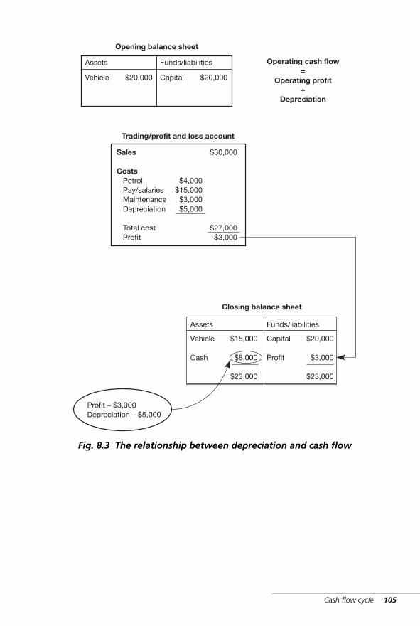
Cash flow cycle 105
Funds/liabilitiesAssets
Capital $20,000Vehicle $20,000
Opening balance sheet
Operating cash flow=
Operating profit+
Depreciation
Trading/profit and loss account
Sales
Costs Petrol Pay/salaries Maintenance Depreciation
Total cost Profit
$4,000$15,000$3,000$5,000
$30,000
$27,000$3,000
Funds/liabilitiesAssets
Capital
Profit
$20,000
$3,000
$23,000
Vehicle
Cash
$15,000
$8,000
$23,000
Closing balance sheet
Profit – $3,000Depreciation – $5,000
Fig. 8.3 The relationship between depreciation and cash flow
WKMR_CH08.QXD 11/24/05 12:20 PM Page 105
Non-operating cash out-flows
In figures 8.1 and 8.2 we saw cash flowing round in a closed circuit. If therewere no leaks from this circuit, there would be few problems. However, thisis not the case and we must now add further sections to the diagram toallow for cash out-flows that are not related to day-to-day operations.
In figure 8.4 the principal additional out-flows are shown as:
■ interest, tax and dividends ■ loan repayments ■ capital expenditure.
We will discuss each in turn.
Interest, tax and dividends
Loan repayments
Capital expenditure
106 Key management ratios
✓
This final item is nearly always a matter of policy. It can probably be deferred inunfavorable circumstances. It is subjected to much thought, analysis and plan-ning. Nevertheless heavy expenditure on projects that do not perform to plan isone of the major causes of cash difficulties.
?
These three items are deducted from EBIT in the ‘profit and loss account’. Theyrepresent a distribution of most of the profit earned for the period. Possibly 75percent of the profit in any year goes out under these headings, to leave approxi-mately 25 percent that is permanently retained in the business.
Therefore we expect cash flow to remain positive even after these charges.Furthermore, as regards timing, the profit is realized in cash well ahead of theseout-flows. So this first set of payments should not, of themselves, be a cause ofcash embarrassment.
?
These can be substantial in amount. They are also deducted from after-taxincome and are in no way connected with the profit for the period. Thereforethey can give rise to heavily negative cash positions. However, the amountsrequired are known well in advance and, in most situations, can be planned andprovided for.
?
WKMR_CH08.QXD 11/24/05 12:20 PM Page 106
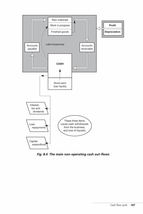
Cash flow cycle 107
Raw materials
Work in progress
Finished goods
Accountspayable
Accountsreceivable
CASH
Short-termloan facility
Profit
Depreciation
Capital expenditure
Loan repayments
Interest, tax and dividends
These three itemscause cash withdrawals
from the business,and loss of liquidity
Labor/expenses
Fig. 8.4 The main non-operating cash out-flows
WKMR_CH08.QXD 11/24/05 12:20 PM Page 107
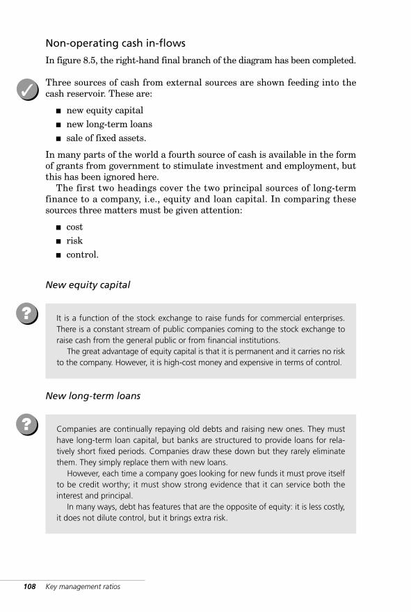
108 Key management ratios
Non-operating cash in-flows
In figure 8.5, the right-hand final branch of the diagram has been completed.
Three sources of cash from external sources are shown feeding into thecash reservoir. These are:
■ new equity capital ■ new long-term loans■ sale of fixed assets.
In many parts of the world a fourth source of cash is available in the formof grants from government to stimulate investment and employment, butthis has been ignored here.
The first two headings cover the two principal sources of long-termfinance to a company, i.e., equity and loan capital. In comparing thesesources three matters must be given attention:
■ cost ■ risk ■ control.
New equity capital
New long-term loans
It is a function of the stock exchange to raise funds for commercial enterprises.There is a constant stream of public companies coming to the stock exchange toraise cash from the general public or from financial institutions.
The great advantage of equity capital is that it is permanent and it carries no riskto the company. However, it is high-cost money and expensive in terms of control.
?
Companies are continually repaying old debts and raising new ones. They musthave long-term loan capital, but banks are structured to provide loans for rela-tively short fixed periods. Companies draw these down but they rarely eliminatethem. They simply replace them with new loans.
However, each time a company goes looking for new funds it must prove itselfto be credit worthy; it must show strong evidence that it can service both theinterest and principal.
In many ways, debt has features that are the opposite of equity: it is less costly,it does not dilute control, but it brings extra risk.
?
✓
WKMR_CH08.QXD 11/24/05 12:20 PM Page 108
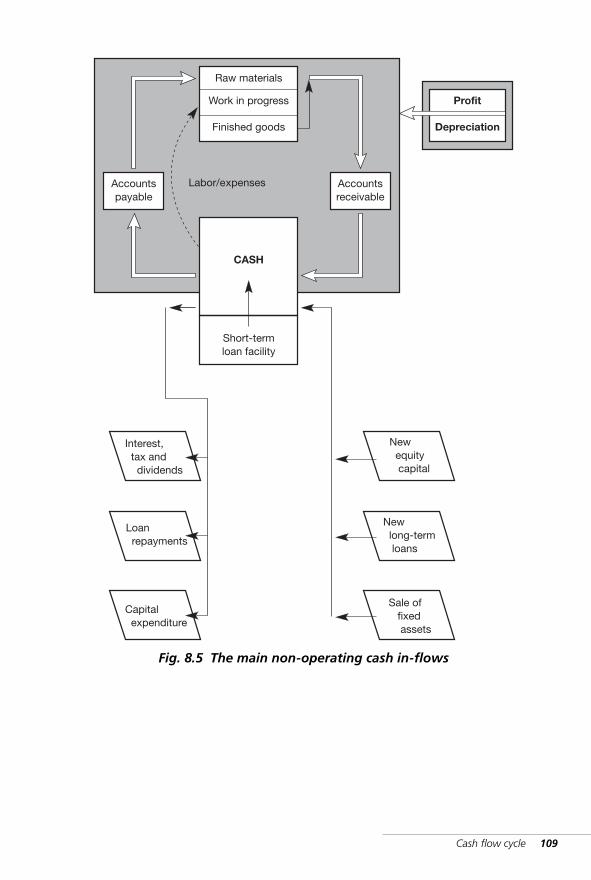
Cash flow cycle 109
Raw materials
Work in progress
Finished goods
Accountspayable
Accountsreceivable
CASH
Short-termloan facility
Profit
Depreciation
Capital expenditure
Loan repayments
Interest, tax and dividends
Sale of fixed assets
New long-term loans
New equity capital
Labor/expenses
Fig. 8.5 The main non-operating cash in-flows
WKMR_CH08.QXD 11/24/05 12:20 PM Page 109
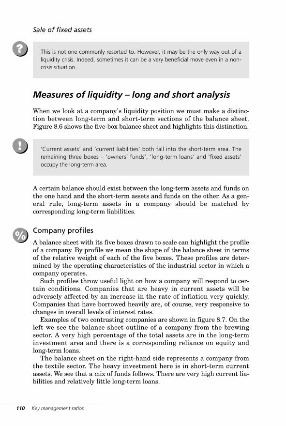
110 Key management ratios
Sale of fixed assets
Measures of liquidity – long and short analysis
When we look at a company’s liquidity position we must make a distinc-tion between long-term and short-term sections of the balance sheet.Figure 8.6 shows the five-box balance sheet and highlights this distinction.
A certain balance should exist between the long-term assets and funds onthe one hand and the short-term assets and funds on the other. As a gen-eral rule, long-term assets in a company should be matched bycorresponding long-term liabilities.
Company profiles
A balance sheet with its five boxes drawn to scale can highlight the profileof a company. By profile we mean the shape of the balance sheet in termsof the relative weight of each of the five boxes. These profiles are deter-mined by the operating characteristics of the industrial sector in which acompany operates.
Such profiles throw useful light on how a company will respond to cer-tain conditions. Companies that are heavy in current assets will beadversely affected by an increase in the rate of inflation very quickly.Companies that have borrowed heavily are, of course, very responsive tochanges in overall levels of interest rates.
Examples of two contrasting companies are shown in figure 8.7. On theleft we see the balance sheet outline of a company from the brewingsector. A very high percentage of the total assets are in the long-terminvestment area and there is a corresponding reliance on equity andlong-term loans.
The balance sheet on the right-hand side represents a company fromthe textile sector. The heavy investment here is in short-term currentassets. We see that a mix of funds follows. There are very high current lia-bilities and relatively little long-term loans.
‘Current assets’ and ‘current liabilities’ both fall into the short-term area. Theremaining three boxes – ‘owners’ funds’, ‘long-term loans’ and ‘fixed assets’occupy the long-term area.
!
%
This is not one commonly resorted to. However, it may be the only way out of aliquidity crisis. Indeed, sometimes it can be a very beneficial move even in a non-crisis situation.
?
WKMR_CH08.QXD 11/24/05 12:20 PM Page 110
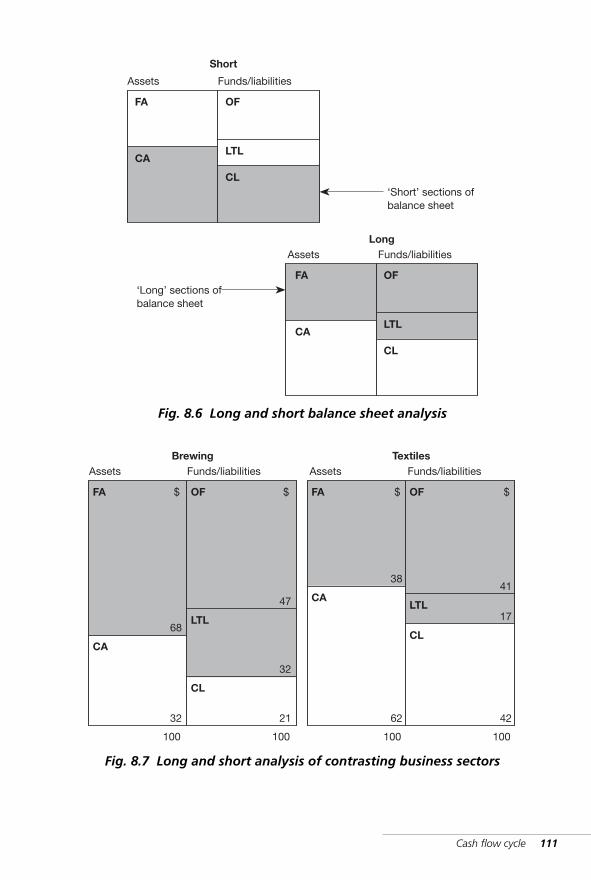
Cash flow cycle 111
Funds/liabilitiesAssets
FA
CA
OF
LTL
CL
Short
Funds/liabilitiesAssets
FA
CA
OF
LTL
CL
Long
‘Short’ sections ofbalance sheet
‘Long’ sections ofbalance sheet
Fig. 8.6 Long and short balance sheet analysis
Funds/liabilitiesAssets
FA
CA
OF
LTL
CL
Brewing
$$
68
32
100
47
32
21
100
Funds/liabilitiesAssets
FA
CA
OF
LTL
CL
Textiles
$$
38
62
100
41
17
42
100
Fig. 8.7 Long and short analysis of contrasting business sectors
WKMR_CH08.QXD 11/24/05 12:20 PM Page 111

WKMR_CH08.QXD 11/24/05 12:20 PM Page 112
9 LiquidityShort-term liquidity measures
· Current ratio · Quick ratio
· Working capital to sales ratio
· Working capital days
Money is the most important thing in theworld. It represents health, strength, honour,generosity and beauty as conspicuously andundeniably as the want of it represents illness,weakness, disgrace, meanness and ugliness.GEORGE BERNARD SHAW (1856–1950)
WKMR_CH09.QXD 11/24/05 12:20 PM Page 113

WKMR_CH09.QXD 11/24/05 12:20 PM Page 114
Liquidity 115
Short-term liquidity measures
Normally short-term liabilities amount to a considerable part of the totalborrowings of the company. They are always greater than the company’spure cash resources. The question we ask is, ‘Where will the cash comefrom to pay them?’
Cash is in constant movement through the company. It flows in dailyfrom accounts receivable as customers pay their bills. Each paymentreduces the balance outstanding, unless it is in turn topped up by trans-fers from the finished goods inventory as new sales are made. Thefinished goods inventory is likewise fed from raw materials and work inprocess. We can visualize these assets as temporary stores for cash, i.e.,inventories in various forms and accounts receivable. These are the assetsthat collectively make up ‘current assets’. They amount to a high percent-age of a company’s total investment.
At the same time, goods are being purchased on credit from suppliers,thereby creating short-term liabilities. Normally other short-term loansare being availed of also. It is these that we collectively refer to as ‘cur-rent liabilities’.
We measure a firm’s short-term liquidity position by comparing thevalues of ‘current assets’ with its ‘current liabilities’.
Three ways of expressing this relationship are illustrated:
■ current ratio ■ quick ratio ■ ‘working capital to sales’ ratio.
We illustrate these measures in this chapter. In chapter 10 measures oflong-term liquidity are discussed.
The first test of a company’s financial position is, ‘Will it have sufficient cash overthe immediate future to meet its short-term liabilities as they fall due?’ Unlessthe answer here is positive, the company is in a financial crisis irrespective of itsprofit performance.
?
✓
WKMR_CH09.QXD 11/24/05 12:20 PM Page 115
116 Key management ratios
Current ratio
The current ratio is a favorite of the institutions that lend money. Thecalculation is based on a simple comparison between the totals of ‘currentassets’ and ‘current liabilities’.
The former represent the amount of liquid, i.e., cash and near-cash,assets available to the business. The latter give an indication of its upcom-ing cash requirements. Institutions expect to see a positive cash surplushere. We therefore look for a value comfortably in excess of 1.0 for thisratio. While this is the standard for most types of businesses, certaintypes of operation are capable of operating at a much lower value.
In figure 9.1 we can see that the average for the US ConsolidatedCompany Inc. in 2000 is 1.3 times. The ‘range of values’ chart for top UKcompanies shows that this ratio can go as high as 1.8 times, and that for asmall percentage of companies it will fall below 1.0 times.
A word of caution is needed concerning the interpretation of this or anyother ratio for a particular company. A wide diversity of conditions exist indifferent types of business. Some businesses are able to exist comfortablywith liquidity ratios that would spell disaster for others. Some companieshave to carry large stocks, have long production cycles, give long creditand so on, while other businesses carry almost no stock and receive morecredit than they give.
One ratio value in isolation tells us little. To get a good picture of a situa-tion we must use a series of tests and we must apply appropriatebenchmarks. These benchmarks can be derived from many sources, suchas historical data, competitors’ accounts and published data of all kinds.
It can be said regarding liquidity ratios, that it is the trend over timerather than the absolute value that gives the most valuable information.A current ratio of 1.2 could give either a good or bad signal depending onpast results.
%
A disadvantage of this ratio is that it does not distinguish between different typesof current assets, some of which are far more liquid than others. A companycould be getting into cash problems and still have a strong current ratio. Thisissue is addressed in the next section.
!
WKMR_CH09.QXD 11/24/05 12:20 PM Page 116
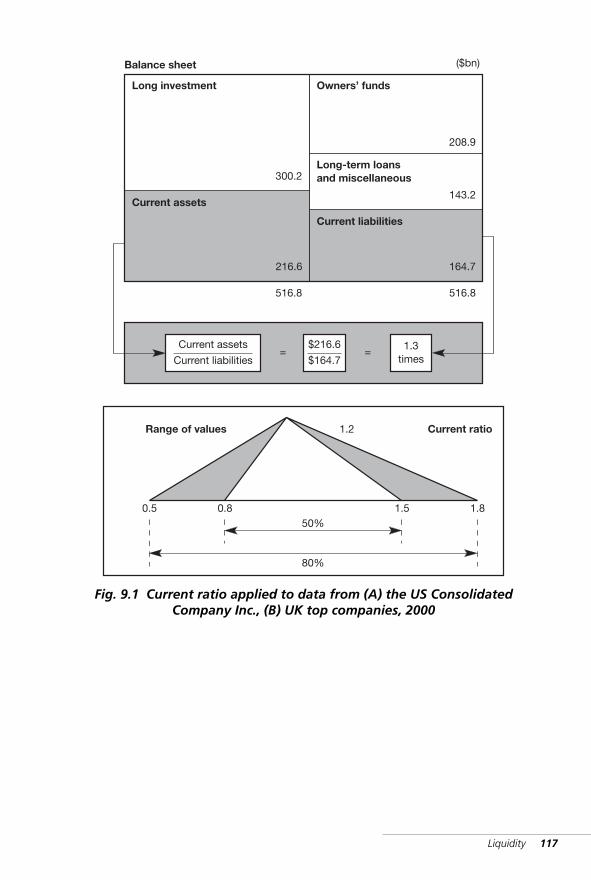
Liquidity 117
Long investment
Current assets
Owners’ funds
Long-term loansand miscellaneous
Current liabilities
300.2
Balance sheet ($bn)
Current assets
Current liabilities=
0.5 0.8 1.5 1.850%
80%
1.2Range of values Current ratio
216.6
516.8
208.9
164.7
516.8
143.2
$216.6
$164.7= 1.3
times
Fig. 9.1 Current ratio applied to data from (A) the US ConsolidatedCompany Inc., (B) UK top companies, 2000
WKMR_CH09.QXD 11/24/05 12:20 PM Page 117
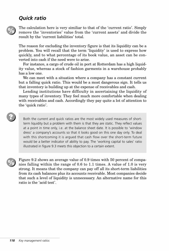
118 Key management ratios
Quick ratio
The calculation here is very similiar to that of the ‘current ratio’. Simplyremove the ‘inventories’ value from the ‘current assets’ and divide theresult by the ‘current liabilities’ total.
The reason for excluding the inventory figure is that its liquidity can be aproblem. You will recall that the term ‘liquidity’ is used to express howquickly, and to what percentage of its book value, an asset can be con-verted into cash if the need were to arise.
For instance, a cargo of crude oil in port at Rotterdam has a high liquid-ity value, whereas a stock of fashion garments in a warehouse probablyhas a low one.
We can meet with a situation where a company has a constant currentbut a falling quick ratio. This would be a most dangerous sign. It tells usthat inventory is building up at the expense of receivables and cash.
Lending institutions have difficulty in ascertaining the liquidity ofmany types of inventory. They feel much more comfortable when dealingwith receivables and cash. Accordingly they pay quite a lot of attention tothe ‘quick ratio’.
Figure 9.2 shows an average value of 0.9 times with 50 percent of compa-nies falling within the range of 0.6 to 1.1 times. A value of 1.0 is verystrong. It means that the company can pay off all its short-term liabilitiesfrom its cash balances plus its accounts receivable. Most companies decidethat such a level of liquidity is unnecessary. An alternative name for thisratio is the ‘acid test’.
Both the current and quick ratios are the most widely used measures of short-term liquidity but a problem with them is that they are static. They reflect valuesat a point in time only, i.e. at the balance sheet date. It is possible to ‘windowdress’ a company’s accounts so that it looks good on this one day only. To dealwith this shortcoming it is argued that cash flow over the short-term futurewould be a better indicator of ability to pay. The ‘working capital to sales’ ratioillustrated in figure 9.3 meets this objection to a certain extent.
?
%
%
WKMR_CH09.QXD 11/24/05 12:20 PM Page 118
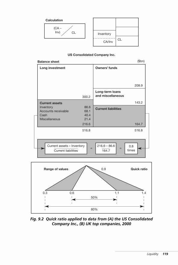
Liquidity 119
Long investment
Current assetsInventoryAccounts receivableCashMiscellaneous
Owners’ funds
Long-term loansand miscellaneous
Current liabilities
300.2
Balance sheet ($bn)
Current assets – Inventory
Current liabilities=
0.3 0.6 1.1 1.450%
80%
0.9Range of values
CA/InvCL
Calculation
Quick ratio
216.6
516.8
208.9
164.7
516.8
143.2
= 0.8times
86.668.140.421.4
216.6 – 86.6
164.7
US Consolidated Company Inc.
Inventory
(CA –Inv) CL
Fig. 9.2 Quick ratio applied to data from (A) the US ConsolidatedCompany Inc., (B) UK top companies, 2000
WKMR_CH09.QXD 11/24/05 12:20 PM Page 119
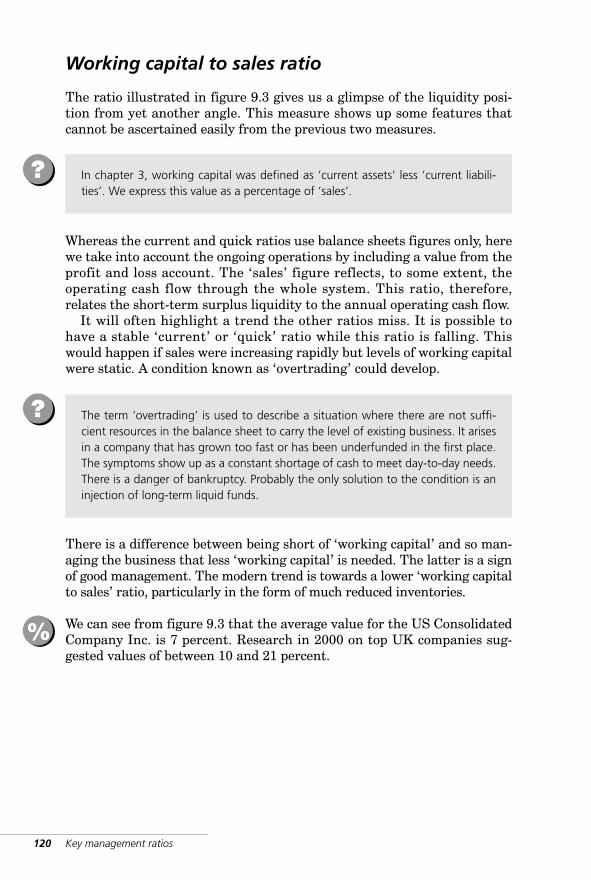
120 Key management ratios
Working capital to sales ratio
The ratio illustrated in figure 9.3 gives us a glimpse of the liquidity posi-tion from yet another angle. This measure shows up some features thatcannot be ascertained easily from the previous two measures.
Whereas the current and quick ratios use balance sheets figures only, herewe take into account the ongoing operations by including a value from theprofit and loss account. The ‘sales’ figure reflects, to some extent, theoperating cash flow through the whole system. This ratio, therefore,relates the short-term surplus liquidity to the annual operating cash flow.
It will often highlight a trend the other ratios miss. It is possible tohave a stable ‘current’ or ‘quick’ ratio while this ratio is falling. Thiswould happen if sales were increasing rapidly but levels of working capitalwere static. A condition known as ‘overtrading’ could develop.
There is a difference between being short of ‘working capital’ and so man-aging the business that less ‘working capital’ is needed. The latter is a signof good management. The modern trend is towards a lower ‘working capitalto sales’ ratio, particularly in the form of much reduced inventories.
We can see from figure 9.3 that the average value for the US ConsolidatedCompany Inc. is 7 percent. Research in 2000 on top UK companies sug-gested values of between 10 and 21 percent.
In chapter 3, working capital was defined as ‘current assets’ less ‘current liabili-ties’. We express this value as a percentage of ‘sales’.
?
The term ‘overtrading’ is used to describe a situation where there are not suffi-cient resources in the balance sheet to carry the level of existing business. It arisesin a company that has grown too fast or has been underfunded in the first place.The symptoms show up as a constant shortage of cash to meet day-to-day needs.There is a danger of bankruptcy. Probably the only solution to the condition is aninjection of long-term liquid funds.
?
%
WKMR_CH09.QXD 11/24/05 12:20 PM Page 120
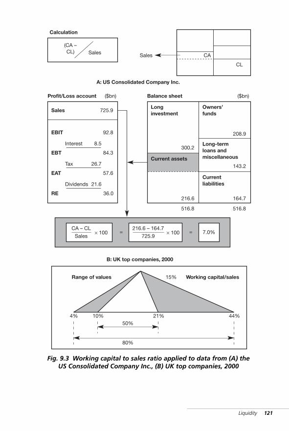
Liquidity 121
Longinvestment
Current assets
Owners’funds
Long-termloans andmiscellaneous
Currentliabilities
300.2
Balance sheet ($bn)
4% 10% 21% 44%50%
80%
15%Range of values
CL
CA
Calculation
Working capital/sales
216.6
516.8
208.9
164.7
516.8
143.2
A: US Consolidated Company Inc.
Sales
Sales
Profit/Loss account ($bn)
725.9
EBIT 92.8
EBT 84.3
EAT 57.6
RE 36.0
8.5Interest
26.7Tax
21.6Dividends
B: UK top companies, 2000
(CA –CL) Sales
CA – CL
Sales= = 7.0%× 100
216.6 – 164.7
725.9× 100
Fig. 9.3 Working capital to sales ratio applied to data from (A) theUS Consolidated Company Inc., (B) UK top companies, 2000
WKMR_CH09.QXD 11/24/05 12:20 PM Page 121
Working capital days
Possibly the clearest way of looking at the role of working capital in acompany’s operations is illustrated in figure 9.4.
Data has been extracted from accounts of the US Consolidated CompanyInc. for ‘inventory’, ‘accounts receivable’ and ‘accounts payable’. The sig-nificance of these accounts is that they are ‘spontaneous’. They react veryquickly to changes in levels of company turnover. The company will havepolicies regarding levels of inventory, etc., but these policies will not fixabsolute values, they will be expressed in terms of sales. A sustainedgrowth in sales will inevitably result in growth in these three accounts.
We express each account in terms of ‘days’ sales’ (see figure 7.5), i.e:
Amount DaysInventory $86.6 (bn) 44Accounts receivable $68.2 34Accounts payable $56.1 28
This data is plotted in figure 9.4. The objective is to show the number ofdays that lapse from the time money is paid out to the suppliers of materi-als until the corresponding cash is received back from the customer thatbuys the goods.
We nominate day 0 to indicate when goods are received from suppliers.Given the average stockholding period, day 44 indicates when the goodsare sold. The customer takes on average 34 days to pay, so cash is receivedon day 78.
In the meantime the company, given its average number of days credit,will have paid the supplier on day 28. The time gap between the cash outon day 28 and its return to the company on day 78 is 50 days. (In additionthe company will have paid out in respect of wages, salaries and over-heads all through the period.)
It is this time gap that creates in a company the need for working capital.The amount is easily quantified. Given a gap of 50 days, each $1m of salesrequires ‘about’ $136,000 ($1m × 50/365) of working capital. Every increaseof $1m will create a need for an additional $136,000 in cash resources. This point is often missed by small rapidly growing companies who findthemselves in cash difficulties in the midst of high sales and profits.
122 Key management ratios
%
WKMR_CH09.QXD 11/24/05 12:20 PM Page 122
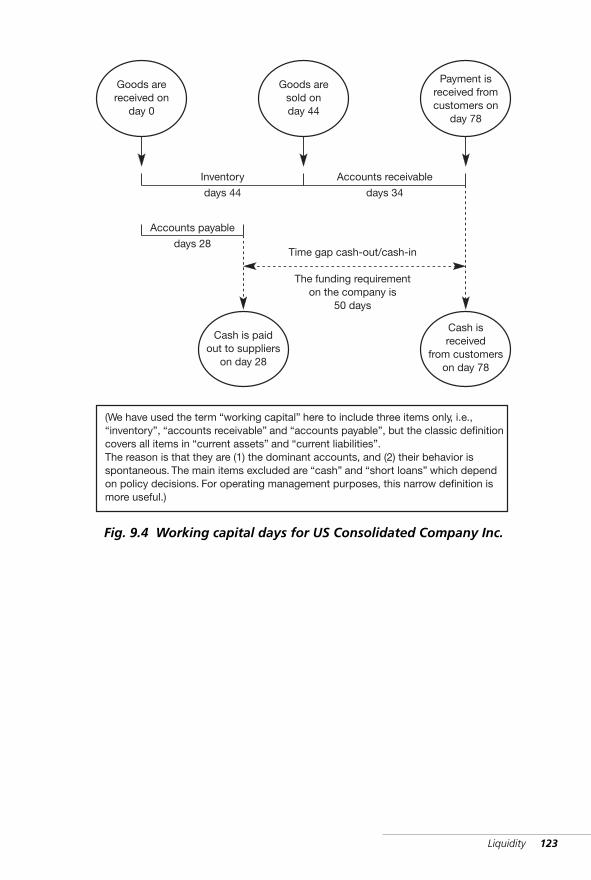
Liquidity 123
Goods arereceived on
day 0
Goods aresold onday 44
Payment isreceived fromcustomers on
day 78
Inventory
days 44
Accounts receivable
days 34
Accounts payable
days 28
Cash is paidout to suppliers
on day 28
Cash isreceived
from customerson day 78
Time gap cash-out/cash-in
The funding requirementon the company is
50 days
(We have used the term “working capital” here to include three items only, i.e.,“inventory”, “accounts receivable” and “accounts payable”, but the classic definitioncovers all items in “current assets” and “current liabilities”.The reason is that they are (1) the dominant accounts, and (2) their behavior isspontaneous. The main items excluded are “cash” and “short loans” which dependon policy decisions. For operating management purposes, this narrow definition ismore useful.)
Fig. 9.4 Working capital days for US Consolidated Company Inc.
WKMR_CH09.QXD 11/24/05 12:20 PM Page 123

WKMR_CH09.QXD 11/24/05 12:20 PM Page 124
10 FinancialstrengthInterest cover · ‘Debt to equity’
ratio (D/E) · Leverage · Summary
Over-trading is among tradesmen as over-lifting is among strong men; such people, vainof their strength…at last lift at somethingtoo heavy for them, over-strain their sinews,break some of nature’s bands and arecripples ever after.DANIEL DEFOE (1660–1731)
WKMR_CH10.QXD 11/24/05 12:21 PM Page 125
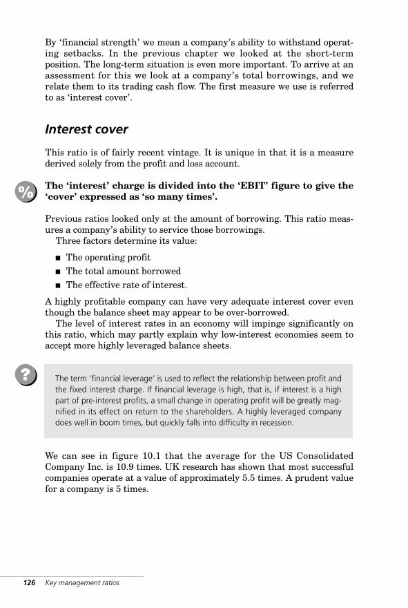
126 Key management ratios
By ‘financial strength’ we mean a company’s ability to withstand operat-ing setbacks. In the previous chapter we looked at the short-termposition. The long-term situation is even more important. To arrive at anassessment for this we look at a company’s total borrowings, and werelate them to its trading cash flow. The first measure we use is referredto as ‘interest cover’.
Interest cover
This ratio is of fairly recent vintage. It is unique in that it is a measurederived solely from the profit and loss account.
The ‘interest’ charge is divided into the ‘EBIT’ figure to give the‘cover’ expressed as ‘so many times’.
Previous ratios looked only at the amount of borrowing. This ratio meas-ures a company’s ability to service those borrowings.
Three factors determine its value:
■ The operating profit■ The total amount borrowed■ The effective rate of interest.
A highly profitable company can have very adequate interest cover eventhough the balance sheet may appear to be over-borrowed.
The level of interest rates in an economy will impinge significantly onthis ratio, which may partly explain why low-interest economies seem toaccept more highly leveraged balance sheets.
We can see in figure 10.1 that the average for the US ConsolidatedCompany Inc. is 10.9 times. UK research has shown that most successfulcompanies operate at a value of approximately 5.5 times. A prudent valuefor a company is 5 times.
%
The term ‘financial leverage’ is used to reflect the relationship between profit andthe fixed interest charge. If financial leverage is high, that is, if interest is a highpart of pre-interest profits, a small change in operating profit will be greatly mag-nified in its effect on return to the shareholders. A highly leveraged companydoes well in boom times, but quickly falls into difficulty in recession.
?
WKMR_CH10.QXD 11/24/05 12:21 PM Page 126
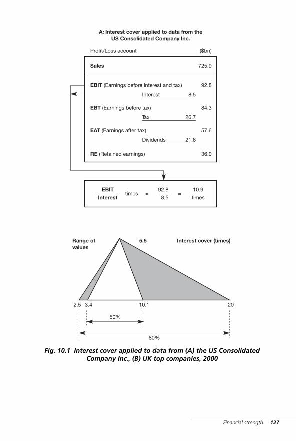
Financial strength 127
Sales
EBIT (Earnings before interest and tax)
Interest 8.5
92.8
EBT (Earnings before tax)
Tax 26.7
84.3
EAT (Earnings after tax)
21.6
57.6
RE (Retained earnings) 36.0
725.9
Profit/Loss account ($bn)
Dividends
EBIT
Interesttimes =
92.8
8.5=
10.9
times
2.5 3.4 10.1 20
Range ofvalues
5.5 Interest cover (times)
50%
80%
A: Interest cover applied to data from theUS Consolidated Company Inc.
Fig. 10.1 Interest cover applied to data from (A) the US ConsolidatedCompany Inc., (B) UK top companies, 2000
WKMR_CH10.QXD 11/24/05 12:21 PM Page 127
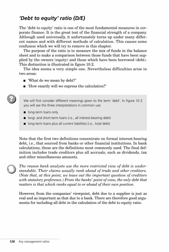
128 Key management ratios
‘Debt to equity’ ratio (D/E)
The ‘debt to equity’ ratio is one of the most fundamental measures in cor-porate finance. It is the great test of the financial strength of a company.Although used universally, it unfortunately turns up under many differ-ent names and with different methods of calculation. This causes someconfusion which we will try to remove in this chapter.
The purpose of the ratio is to measure the mix of funds in the balancesheet and to make a comparison between those funds that have been sup-plied by the owners (equity) and those which have been borrowed (debt).This distinction is illustrated in figure 10.2.
The idea seems a very simple one. Nevertheless difficulties arise intwo areas:
■ ‘What do we mean by debt?’ ■ ‘How exactly will we express the calculation?’
Note that the first two definitions concentrate on formal interest-bearingdebt, i.e., that sourced from banks or other financial institutions. In bankcalculations, these are the definitions most commonly used. The final def-inition includes trade creditors plus all accruals, such as dividends, taxand other miscellaneous amounts.
The reason bank analysts use the more restricted view of debt is under-standable. Their claims usually rank ahead of trade and other creditors.(Note that, at this point, we leave out the important question of creditorswith statutory preference.) From the banks’ point of view, the only debt thatmatters is that which ranks equal to or ahead of their own position.
However, from the companies’ viewpoint, debt due to a supplier is just asreal and as important as that due to a bank. There are therefore good argu-ments for including all debt in the calculation of the debt to equity ratio.
We will first consider different meanings given to the term ‘debt’. In figure 10.3you will see the three interpretations in common use:
■ long-term loans only
■ long- and short-term loans (i.e., all interest-bearing debt)
■ long-term loans plus all current liabilities (i.e., total debt)
?
WKMR_CH10.QXD 11/24/05 12:21 PM Page 128
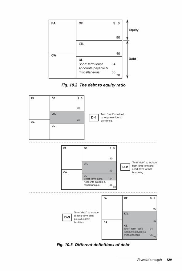
Financial strength 129
70
40
90
FA
CA
OF
LTL
CLShort-term loansAccounts payable &miscellaneous
$ $
34
36
Equity
Debt
Fig. 10.2 The debt to equity ratio
Term “debt” confinedto long-term formalborrowing.
Term “debt” to includeboth long-term andshort-term formalborrowing.
Term “debt” to includeall long-term debtplus all currentliabilities.
FA
CA
OF
LTL
CL
$ $
70
FA
CA
OF
LTL
CLShort-term loansAccounts payable &miscellaneous
$ $
34
36
70
40
90
FA
CA
OF
LTL
CLShort-term loansAccounts payable &miscellaneous
$ $
34
36
D-1
D-2
D-3
90
40
90
40
Fig. 10.3 Different definitions of debt
WKMR_CH10.QXD 11/24/05 12:21 PM Page 129
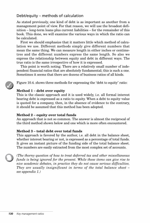
130 Key management ratios
Debt/equity – methods of calculation
As stated previously, one kind of debt is as important as another from amanagement point of view. For that reason, we will use the broadest defi-nition – long-term loans plus current liabilities – for the remainder of thisbook. This done, we will examine the various ways in which the ratio canbe calculated.
First we should emphasize that it matters little which method of calcu-lation we use. Different methods simply give different numbers thatmean the same thing. We can measure length in either inches or centime-tres and the different numbers express the same length. So also weexpress the relationship between equity and debt in different ways. Thetrue ratio is the same irrespective of how it is expressed.
This point is worth noting. There are a relatively small number of inde-pendent financial ratios that are absolutely fundamental; this is such a one.Sometimes it seems that there are dozens of business ratios of all kinds.
Figure 10.4. shows three methods for expressing the ‘debt to equity’ ratio:
Method 1 – debt over equity This is the classic approach and it is used widely, i.e. all formal interestbearing debt is expressed as a ratio to equity. When a debt to equity valueis quoted for a company, then, in the absence of evidence to the contrary,it should be assumed that this method has been adopted.
Method 2 – equity over total funds An approach that is not so common. The answer is almost the reciprocal ofthe third method shown below and one which is more often encountered.
Method 3 – total debt over total funds This approach is favored by the author, i.e. all debt in the balance sheet,whether interest bearing or not, is expressed as a percentage of total funds.It gives an instant picture of the funding side of the total balance sheet.The numbers are easily extracted from the most complex set of accounts.
(The thorny question of how to treat deferred tax and other miscellaneousfunds is being ignored for the present. While these items can give rise tonice academic debates, in practice they do not cause serious difficulties.They are usually insignificant in terms of the total balance sheet –see appendix 1.)
✓
WKMR_CH10.QXD 11/24/05 12:21 PM Page 130
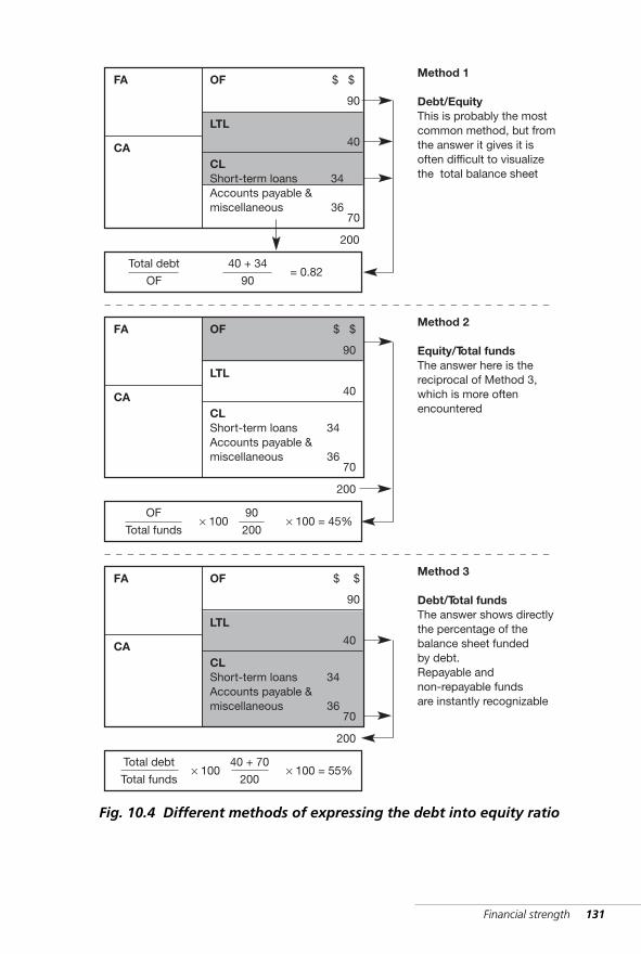
Financial strength 131
Method 1
Debt/EquityThis is probably the mostcommon method, but fromthe answer it gives it isoften difficult to visualizethe total balance sheet
70
40
90
FA
CA
OF
LTL
CLShort-term loansAccounts payable &miscellaneous
$ $
34
36
Total debt
OF
40 + 34
90= 0.82
200
Method 2
Equity/Total fundsThe answer here is thereciprocal of Method 3,which is more oftenencountered
70
40
FA
CA
OF
LTL
CLShort-term loansAccounts payable &miscellaneous
$ $
34
36
OF
Total funds
90
200× 100 = 45%
200
Method 3
Debt/Total fundsThe answer shows directlythe percentage of thebalance sheet fundedby debt.Repayable andnon-repayable fundsare instantly recognizable
70
40
FA
CA
OF
LTL
CLShort-term loansAccounts payable &miscellaneous
$ $
34
36
200
90
90
× 100
Total debt
Total funds
40 + 70
200× 100 = 55%× 100
Fig. 10.4 Different methods of expressing the debt into equity ratio
WKMR_CH10.QXD 11/24/05 12:21 PM Page 131
132 Key management ratios
%
Debt/equity – why it is important
The greater the debt, the greater the risk. All debt in the balance sheetgives third parties legal claims on the company. These claims are forinterest payments at regular intervals, plus repayment of the principal bythe agreed time. The principal is repaid either by periodic instalments ora single lump sum at the end of the loan period.
Therefore when a company raises debt, it takes on a commitment tosubstantial fixed cash out-flows for some time into the future. The com-pany does not have a guaranteed cash in-flow over the same period.Indeed the in-flow may be most uncertain. A fixed cash out-flow com-bined with an uncertain cash in-flow gives rise to financial risk. It followsthat the greater the loan, the greater is the risk.
Why, then, do companies take on debt and incur this extra risk? Theanswer lies in the relative costs. Debt costs less than equity funds. Byadding debt to its balance sheet, a company can generally improve itsprofitability, add to its share price, increase the wealth of its shareholdersand develop greater potential for growth.
Where should the line be drawn? The increased return to the equityshareholder that results from debt leverage can rarely be forsaken alto-gether even though some companies do just that. Most companies musttake a view on the degree of uncertainty of future cash receipts andarrange their level of debt in line with this uncertainty.
We find that companies in business sectors with very predictableincome streams, e.g. property leasing, incur high levels of debt. Companiesin highly volatile sectors, e.g. mine exploration, fund mainly from equity.
We find geographical as well as sectoral differences in companies’approach to debt (see figure 10.5). In the US as well as in the UK theapproach is more conservative than we find in the EU. In the former loca-tions it is unusual for debt/total assets to exceed 60 percent. In the latterwe often encounter ratios of 70 percent and over.
We place a lot of emphasis on this ratio because, if it goes wrong, the companyhas a real long-term problem; one which may become terminal.
!
Debt increases both profit and risk. It is the job of management to maintain aproper balance between the two.
!
WKMR_CH10.QXD 11/24/05 12:21 PM Page 132
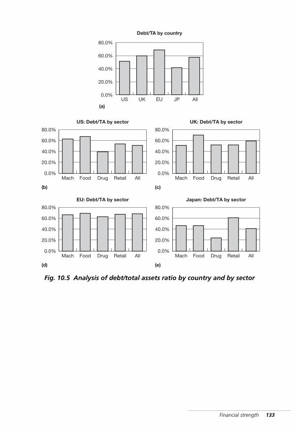
Financial strength 133
80.0%
60.0%
40.0%
20.0%
0.0%
EU: Debt/TA by sector
(d)
Mach Food Drug Retail All
80.0%
60.0%
40.0%
20.0%
0.0%
Japan: Debt/TA by sector
(e)
Mach Food Drug Retail All
80.0%
20.0%
0.0%US
Debt/TA by country
(a)UK EU JP All
60.0%
40.0%
80.0%
60.0%
40.0%
20.0%
0.0%
US: Debt/TA by sector
(b)
Mach Food Drug Retail All
80.0%
60.0%
40.0%
20.0%
0.0%
UK: Debt/TA by sector
(c)
Mach Food Drug Retail All
Fig. 10.5 Analysis of debt/total assets ratio by country and by sector
WKMR_CH10.QXD 11/24/05 12:21 PM Page 133
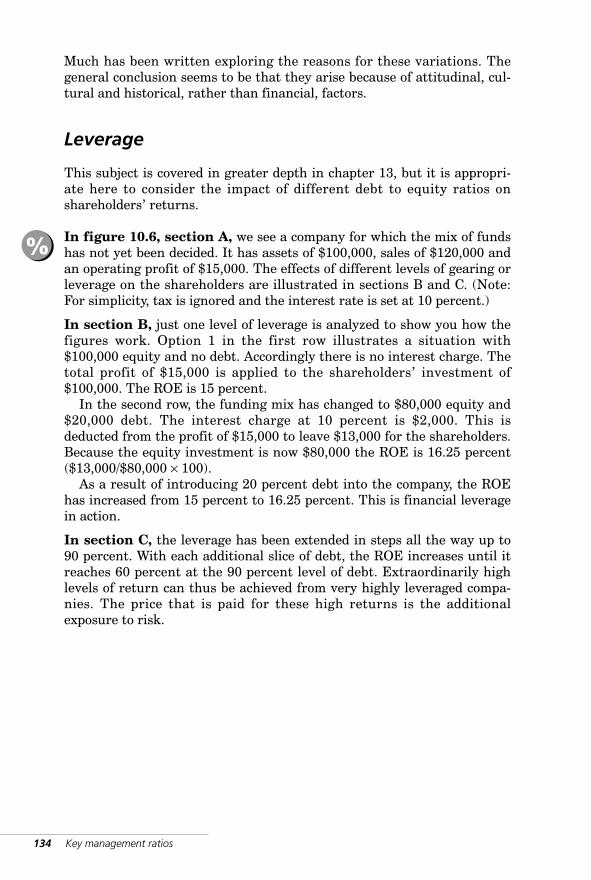
134 Key management ratios
Much has been written exploring the reasons for these variations. Thegeneral conclusion seems to be that they arise because of attitudinal, cul-tural and historical, rather than financial, factors.
Leverage
This subject is covered in greater depth in chapter 13, but it is appropri-ate here to consider the impact of different debt to equity ratios onshareholders’ returns.
In figure 10.6, section A, we see a company for which the mix of fundshas not yet been decided. It has assets of $100,000, sales of $120,000 andan operating profit of $15,000. The effects of different levels of gearing orleverage on the shareholders are illustrated in sections B and C. (Note:For simplicity, tax is ignored and the interest rate is set at 10 percent.)
In section B, just one level of leverage is analyzed to show you how thefigures work. Option 1 in the first row illustrates a situation with$100,000 equity and no debt. Accordingly there is no interest charge. Thetotal profit of $15,000 is applied to the shareholders’ investment of$100,000. The ROE is 15 percent.
In the second row, the funding mix has changed to $80,000 equity and$20,000 debt. The interest charge at 10 percent is $2,000. This isdeducted from the profit of $15,000 to leave $13,000 for the shareholders.Because the equity investment is now $80,000 the ROE is 16.25 percent($13,000/$80,000 × 100).
As a result of introducing 20 percent debt into the company, the ROEhas increased from 15 percent to 16.25 percent. This is financial leveragein action.
In section C, the leverage has been extended in steps all the way up to90 percent. With each additional slice of debt, the ROE increases until itreaches 60 percent at the 90 percent level of debt. Extraordinarily highlevels of return can thus be achieved from very highly leveraged compa-nies. The price that is paid for these high returns is the additionalexposure to risk.
%
WKMR_CH10.QXD 11/24/05 12:21 PM Page 134
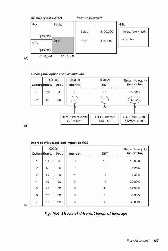
Financial strength 135
F/A
C/ADebt
$60,000
$40,000
Equity
$100,000 $100,000
Balance sheet extract
Sales
Profit/Loss extract
$120,000
EBIT $15,000
Interest rate = 10%
Ignore tax
N.B.
1
2
100
80
0
20
Equity Debt
($000s)
0
2
Interest
($000s)
15
13
EBT
($000s)
15.00%
16.25%
Return to equity(before tax)
EBT/Equity × 100$13/$80 × 100
EBIT – Interest$15 – $2
Debt × Interest rate$20 × 10%
Funding mix options and calculations
1
2
3
4
5
6
7
100
80
60
50
40
20
10
0
20
40
50
60
80
90
Equity Debt
($000s)
0
2
4
5
6
8
9
Interest
15
13
11
10
9
7
6
EBT
15.00%
16.25%
18.33%
20.00%
22.50%
35.00%
60.00%
Return to equity(before tax)
Degrees of leverage and impact on ROE
Option
Option
(A)
(B)
(C)
Fig. 10.6 Effects of different levels of leverage
WKMR_CH10.QXD 11/24/05 12:21 PM Page 135
136 Key management ratios
Summary
The debt/equity or leverage decision is one of great importance to man-agement. There is a risk return trade-off. The impulse to achieve highreturns for the shareholders must be restrained by the company’s riskprofile. Even a very well managed company can suffer an unexpecteddeterioration in its financial position either from a default on the part of amajor debtor or a general worsening of business conditions. Such a deteri-oration can be very difficult to recover from. It is prudent to keep someliquidity in reserve to guard against such an eventuality.
☛
WKMR_CH10.QXD 11/24/05 12:21 PM Page 136
11 Cash flowThe cash flow statement · Sources
and uses of funds – method ·Opening and closing cash
reconciliation · Long and short
analysis · Financial reporting
standards
But when times are bad and the breath offear has already chilled the markets, thebanker must be cautious, conservative, andsevere. His business has been aptly comparedto that of a man who stands ready to lendumbrellas when it is fine and demand themback when it starts to rain.SIR GEOFFREY CROWTHER (1907–1972)
WKMR_CH11.QXD 11/24/05 12:21 PM Page 137

WKMR_CH11.QXD 11/24/05 12:21 PM Page 138
Cash flow 139Cash flow 139
The cash flow statement
There are those who would contend that the cash flow statement is morereliable and less subject to manipulation than the profit and loss account.
Many operating cash movements do not appear in the profit and lossaccount. One reason is that the profit and loss account uses the accrualsconcept to adjust a company’s cash flows to bring them into line with rev-enue earned and costs incurred for a specific period. While it is mostimportant that true revenue and costs are identified, these adjustmentssometimes hide important aspects of a company’s affairs.
The cash flow statement has in the past been presented in manyformats, but it has now been standardized into the layout shown (inslightly simplified form) in figure 11.6.
However, despite its clarity, it cannot, as is occasionally suggested, replacethe profit and loss account. The latter correctly distinguishes betweencash paid for electricity consumed last month and cash paid for a buildingthat will be occupied by the company for the next 20 years.
This chapter looks at the logic of the cash flow statement and how itcan be of use to management.
The cash flow statement completes a company’s set of published accounts. Itspurpose is to track the flow of funds through the company. It identifies wherecash has gone to and where it has come from and it is a very powerful tool forexplaining movements in the various liquidity ratios.
?
The rules relating to cash flow are very simple. Every time a company writes acheque, a cash out-flow occurs. When a cheque is received, there is a cash in-flow. This is the only rule, and its very simplicity means that it is difficult to findmechanisms to hide unpleasant truths about a company’s affairs.
!
WKMR_CH11.QXD 11/24/05 12:21 PM Page 139
140 Key management ratios Cash flow 140
Sources and uses of funds – method
To get at the data needed in order to build a cash flow statement, we gothrough a sources and uses exercise. The mechanics of this exercise areeasy to grasp and are shown in figure 11.1 opposite.
In figure 11.1 a simplified balance sheet is shown for the two years 2000and 2001. It has been laid out in vertical columns to facilitate comparisonbetween the two years. The assets are in the upper section of the state-ment and the liabilities in the lower. To the right of the balance sheet, twoextra columns have been added – respectively ‘Source’ and ‘Use’.
An entry will be made in one of these columns for every change that hastaken place in a balance sheet item.
■ If the change has caused a cash out-flow, the entry will be entered inthe ‘Use’column.
■ For a cash in-flow, the entry will be made in the ‘Source’ column.
Two entries have been illustrated:
1 Fixed assets $10,000 Use of funds
2 Tax $500 Source of funds
The logic of the first entry is fairly obvious. The fixed assets haveincreased from $22,500 to $32,500. The company has had to write acheque for $10,000. (For the purposes of this exercise we ignore revalua-tion and depreciation.)
The second entry is less obvious. The amount shown under ‘Tax’ hasincreased from $2,500 to $3,000. How can an increase in tax be a source offunds? The answer is that the tax amount of $3,000 shown as a liability inthe closing balance sheet is unpaid. The company now has the use of $500more government money than it had one year ago, so for the present it is asource of funds. This liability will have to be paid off in due course. It willthen disappear from the balance sheet and be picked up as a use of funds.
%
WKMR_CH11.QXD 11/24/05 12:21 PM Page 140
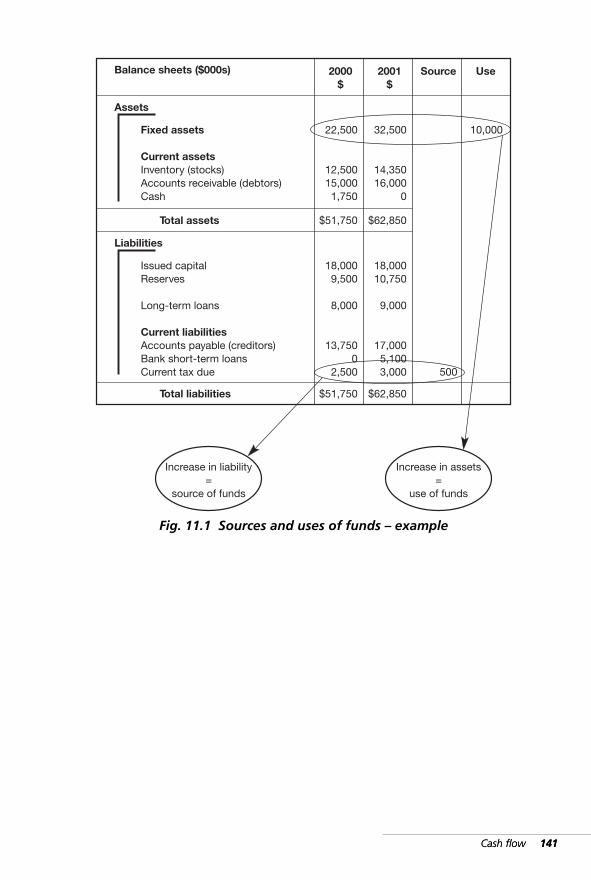
Cash flow 141Cash flow 141
Balance sheets ($000s)
Assets
Fixed assets
Current assetsInventory (stocks)Accounts receivable (debtors)Cash
Total assets
Liabilities
Issued capitalReserves
Long-term loans
Current liabilitiesAccounts payable (creditors)Bank short-term loansCurrent tax due
Total liabilities
2000$
22,500
12,50015,0001,750
2001$
32,500
14,35016,000
0
Source Use
10,000
$51,750 $62,850
18,0009,500
8,000
13,7500
2,500
18,00010,750
9,000
17,0005,1003,000
$51,750 $62,850
Increase in liability=
source of funds
Increase in assets=
use of funds
500
Fig. 11.1 Sources and uses of funds – example
WKMR_CH11.QXD 11/24/05 12:21 PM Page 141
142 Key management ratios Cash flow 142
Rules of construction
The completed statement is shown in figure 11.2. All changes in balancesheet values have been identified and classified as sources or uses. Thetotal sources agree with the total uses. This will always be the case.
It can be difficult at first to distinguish sources from uses and to putitems into the wrong columns. Fortunately there is a rule that makes theclassification very simple:
Increase DecreaseAsset Use SourceLiability Source Use
Therefore to complete the statement one simply needs to identify a changein any balance sheet value and answer the the following questions:
■ ‘Is the item an asset or liability?’■ ‘Has its value increased or decreased?’
then the item automatically slots into its correct column.
The exercise illustrates a technique for translating all balance sheetchanges into corresponding movements of funds. The reader will appreci-ate that this method does not in fact identify all cash payments and allcash receipts. What it does is track net movements in assets and liabilitiesthat will impinge on a company’s cash position. The method demon-strated is called the ‘indirect method’.*
Hidden movements
A word of caution is needed here. The indirect method picks up only thenet movements in balance sheet values. Of course a net change can be theresult of two opposing movements that partly cancel out. A full cash flowstatement should pick such items. Even more importantly some movementsin balance sheet values do not give rise to cash flow – revaluation of fixedassets is an example (see appendix 1). It may be necessary to get behindsome of the numbers to find out if there are any hidden or non-cash move-ments. Notwithstanding these qualifications, the method illustrated hereis a powerful tool of analysis.
* One sometimes sees a ‘payments and receipts’ form of cash statement that gives sum-maries of all cheques paid and received. Such a statement has little analytical value but iscrucial for control purposes.
☛
WKMR_CH11.QXD 11/24/05 12:21 PM Page 142
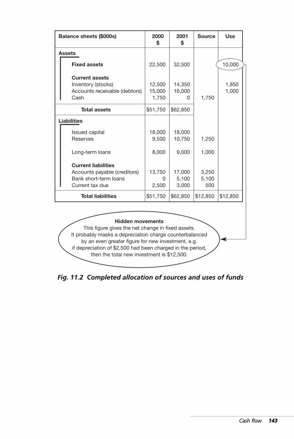
Cash flow 143Cash flow 143
Balance sheets ($000s)
Assets
Fixed assets
Current assetsInventory (stocks)Accounts receivable (debtors)Cash
Total assets
Liabilities
Issued capitalReserves
Long-term loans
Current liabilitiesAccounts payable (creditors)Bank short-term loansCurrent tax due
Total liabilities
2000$
22,500
12,50015,0001,750
2001$
32,500
14,35016,000
0
Source Use
$51,750 $62,850
18,0009,500
8,000
13,7500
2,500
18,00010,750
9,000
17,0005,1003,000
$51,750 $62,850
Hidden movementsThis figure gives the net change in fixed assets.
It probably masks a depreciation charge counterbalancedby an even greater figure for new investment, e.g.
if depreciation of $2,500 had been charged in the period,then the total new investment is $12,500.
1,750
1,8501,000
1,250
1,000
3,2505,100
500
$12,850 $12,850
10,000
Fig. 11.2 Completed allocation of sources and uses of funds
WKMR_CH11.QXD 11/24/05 12:21 PM Page 143
144 Key management ratios Cash flow 144
Opening and closing cash reconciliation
Once the sources and uses have been identified and reconciled, we can usevarious layouts of the cash flow statement to draw management’s atten-tion to specific issues.
For instance, the company’s cash position could deteriorate eventhough high profits have been achieved. To explain why, we could use alayout that would reconcile opening and closing cash with the net cashflow for the period. It would show:
■ the opening cash balance,■ the itemized cash out-flows,■ the itemized cash in-flows,■ the closing cash balance.
The layout shown in figure 11.3 illustrates such a reconciliation.
(Note: A cash balance can be positive or negative. A positive position is wherethere is cash asset whereas a negative position shows up as short-term bank loan.)
The various entries are taken straight from the ‘sources/uses’ statement(see figure 11.2). ‘Cash-out’ items are taken from the ‘use’ column and‘cash-in’ from the ‘source’ column. There is one exception to this rule:movements in ‘cash’ and ‘short loan’ are not listed because they areabsorbed in the ‘opening/closing’ cash positions.
■ The total for cash-out comes to: $12,850 (negative)■ The total for cash-in comes to: $ 6,000 (positive)■ The net cash flow is the difference: $ 6,850 (negative)
This net cash flow, added to the opening cash figure of $1,750 (positive)gives the closing cash position of $5,100 (negative).
The statement clearly identifies major movements in the cash position.Even a cursory examination of the figures shows the reason for the nega-tive cash flow. The company has expended $10,000 on fixed assets. Thisrelatively large sum has not been matched by any corresponding large cashin-flows. The assets have been purchased from day-to-day operating cash.
The heavily negative net cash flow also explains why the ‘current ratio’has dropped from 1.8 to 1.2 times, and the ‘debt to total assets’ ratio ofthe company has increased from 47 percent to 54 percent.
This issue is pursued further in the next section.
☛
%
WKMR_CH11.QXD 11/24/05 12:21 PM Page 144
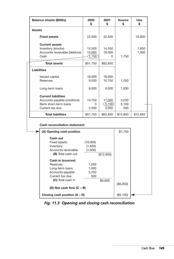
Cash flow 145Cash flow 145
Balance sheets ($000s)
Assets
Fixed assets
Current assetsInventory (stocks)Accounts receivable (debtors)Cash
Total assets
Liabilities
Issued capitalReserves
Long-term loans
Current liabilitiesAccounts payable (creditors)Bank short-term loansCurrent tax due
Total liabilities
2000$
22,500
12,50015,0001,750
2001$
32,500
14,35016,000
0
Source$
Use$
$51,750 $62,850
18,0009,500
8,000
13,7500
2,500
18,00010,750
9,000
17,0005,1003,000
$51,750 $62,850
1,750
1,8501,000
1,250
1,000
3,2505,100
500
$12,850 $12,850
10,000
(A) Opening cash position
Cash outFixed assetsInventoryAccounts receivable (B) Total cash out
Cash in (sources)ReservesLong-term loansAccounts payableCurrent tax due (C) Total cash in
(D) Net cash flow (C – B)
Closing cash position (A – D)
(10,000)(1,850)(1,000)
1,2501,0003,250
500
($12,850)
$6,000
$1,750
($6,850)
($5,100)
Cash reconciliation statement
Fig. 11.3 Opening and closing cash reconciliation
WKMR_CH11.QXD 11/24/05 12:21 PM Page 145
146 Key management ratios Cash flow 146
Long and short analysis
The information provided in figure 11.3 adds considerably to knowledgeof the company’s affairs that we could have derived from the balancesheet and profit and loss account. Alternative layouts of the cash flowdata provide more insights.
In figure 11.4, the same original data has been plotted into a grid that dis-tinguishes between ‘long’ and ‘short’ sources on the one hand, and ‘long’and ‘short’ uses on the other (refer back to page 111 where the ‘long’ and‘short’ sections of the balance sheet were identified).
Each item in the ‘Source’ column has been slotted into its appropriate‘long’ or ‘short’ box. Ditto for all items in the ‘Use’ column. The boxes aretotaled to give four major values for comparison.
The main expenditure has taken place in the ‘Long-Use’ box. We iden-tify here the large fixed asset purchase of $10,000.
The corresponding ‘Long-Source’ box shows $2,250. The total amountof long-term cash received into the business by way of ‘Reserves’ and the‘Long-term loans’ falls considerably short of the fixed asset expenditure.
Because ‘sources’ and ‘uses’ must balance, the above deficit must bemade good from the ‘Short-Source’ box. We see that this is indeed thecase. The bulk of the cash in-flow falls into the short-term box.
Most of the money that has come into the business has come from‘accounts payable’ and ‘bank loan’. These are due to be repaid within 12months. The company has used short-term sources to fund long-termassets.
This layout of the cash flow highlights the fact that ‘current liabilities’have increased by much more than ‘current assets’ and has brought aboutthe deterioration we have already seen in the ‘current ratio’.
The ‘debt to total assets ratio’ has also deteriorated over the 2000–01period. This is analyzed in further detail in the next section.
%
WKMR_CH11.QXD 11/24/05 12:21 PM Page 146
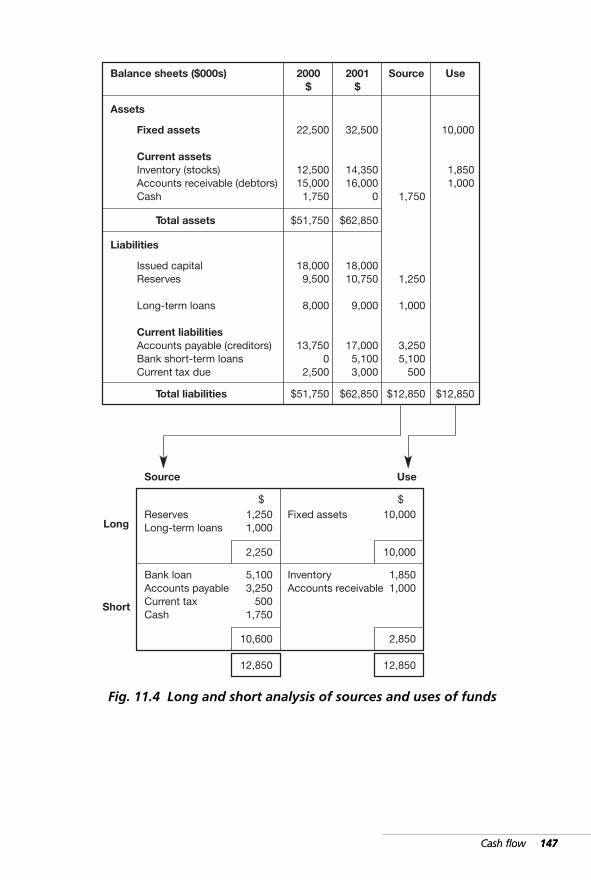
Cash flow 147Cash flow 147
Balance sheets ($000s)
Assets
Fixed assets
Current assetsInventory (stocks)Accounts receivable (debtors)Cash
Total assets
Liabilities
Issued capitalReserves
Long-term loans
Current liabilitiesAccounts payable (creditors)Bank short-term loansCurrent tax due
Total liabilities
2000$
22,500
12,50015,0001,750
2001$
32,500
14,35016,000
0
Source Use
$51,750 $62,850
18,0009,500
8,000
13,7500
2,500
18,00010,750
9,000
17,0005,1003,000
$51,750 $62,850
1,750
1,8501,000
1,250
1,000
3,2505,100
500
$12,850 $12,850
10,000
Source
ReservesLong-term loans
1,2501,000
$
2,250
Fixed assets 10,000
10,000
Bank loanAccounts payableCurrent taxCash
10,600
InventoryAccounts receivable
1,8501,000
2,850
Use
Long
Short
12,850 12,850
$
5,1003,250
5001,750
Fig. 11.4 Long and short analysis of sources and uses of funds
WKMR_CH11.QXD 11/24/05 12:21 PM Page 147
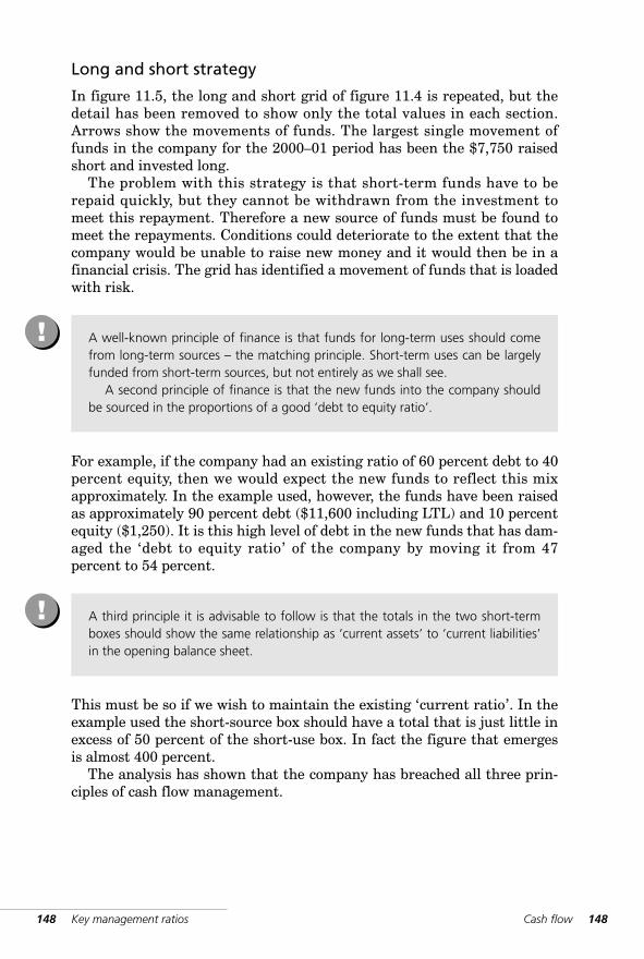
148 Key management ratios Cash flow 148
Long and short strategy
In figure 11.5, the long and short grid of figure 11.4 is repeated, but thedetail has been removed to show only the total values in each section.Arrows show the movements of funds. The largest single movement offunds in the company for the 2000–01 period has been the $7,750 raisedshort and invested long.
The problem with this strategy is that short-term funds have to berepaid quickly, but they cannot be withdrawn from the investment tomeet this repayment. Therefore a new source of funds must be found tomeet the repayments. Conditions could deteriorate to the extent that thecompany would be unable to raise new money and it would then be in afinancial crisis. The grid has identified a movement of funds that is loadedwith risk.
For example, if the company had an existing ratio of 60 percent debt to 40percent equity, then we would expect the new funds to reflect this mixapproximately. In the example used, however, the funds have been raisedas approximately 90 percent debt ($11,600 including LTL) and 10 percentequity ($1,250). It is this high level of debt in the new funds that has dam-aged the ‘debt to equity ratio’ of the company by moving it from 47percent to 54 percent.
This must be so if we wish to maintain the existing ‘current ratio’. In theexample used the short-source box should have a total that is just little inexcess of 50 percent of the short-use box. In fact the figure that emergesis almost 400 percent.
The analysis has shown that the company has breached all three prin-ciples of cash flow management.
A well-known principle of finance is that funds for long-term uses should comefrom long-term sources – the matching principle. Short-term uses can be largelyfunded from short-term sources, but not entirely as we shall see.
A second principle of finance is that the new funds into the company shouldbe sourced in the proportions of a good ‘debt to equity ratio’.
!
A third principle it is advisable to follow is that the totals in the two short-termboxes should show the same relationship as ‘current assets’ to ‘current liabilities’in the opening balance sheet.
!
WKMR_CH11.QXD 11/24/05 12:21 PM Page 148
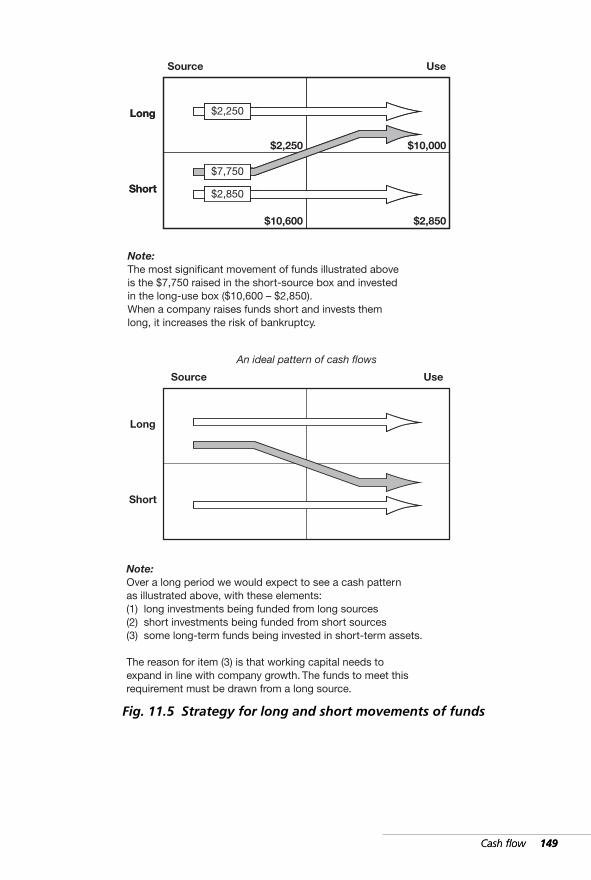
Cash flow 149Cash flow 149
Source Use
Long
Short
Note:The most significant movement of funds illustrated aboveis the $7,750 raised in the short-source box and investedin the long-use box ($10,600 – $2,850).When a company raises funds short and invests themlong, it increases the risk of bankruptcy.
Note:Over a long period we would expect to see a cash patternas illustrated above, with these elements:(1) long investments being funded from long sources(2) short investments being funded from short sources(3) some long-term funds being invested in short-term assets.
The reason for item (3) is that working capital needs toexpand in line with company growth. The funds to meet thisrequirement must be drawn from a long source.
Use
Long
Short
$10,000
£2, 250
£2, 850
£2, 250
Source
Long
Short
$2,850$10,600
$2,250
$2,850
$7,750
$2,250
An ideal pattern of cash flows
Fig. 11.5 Strategy for long and short movements of funds
WKMR_CH11.QXD 11/24/05 12:21 PM Page 149
Financial reporting standards
In recent years there have been a number of highly publicized situationswhere it emerged after the event that fully audited published financial state-ments had not provided satisfactory information to the investors or bankersinvolved. Criticism has been voiced of existing standards of reporting.
As a result the Financial Accounting Standards Boards (FASB) of thevarious developed countries have stepped up their efforts to impose morerigorous reporting standards. The cash flow statement has been one toreceive particular attention.
Phrases such as: ‘to give users information on the liquidity, viabilityand financial adaptability of the entity concerned,’; ‘improved under-standing of a reporting entity’s cash generating or cash absorptionmechanisms,’; ‘basis for the assessment of future cash flow,’ give a flavorof the desired objectives.
The standards arrived at lay great stress on identifying the followingseparate components of the flow of cash and its equivalents:
■ operating activities ■ servicing of finance and taxation ■ investing activities ■ financing activities.
They further require a reconciliation of the figure shown for operatingprofit and operating cash flow, as well as a total showing the net cash in-flow or out-flow before financing.
Figure 11.6 identifies the main headings but omits much of the detailin the interest of clarity.
The terminology in the Reporting Standards will be widely used in board-rooms and management meetings over the coming years. It is importantthat managers be familiar with this terminology and appreciate the signifi-cance of the various components of cash flow. The sources and usesstatement has been dropped as a reporting requirement, but it still remainsa powerful tool of analysis for managers to use for their own benefit.
150 Key management ratios
✓
☛
WKMR_CH11.QXD 11/24/05 12:21 PM Page 150
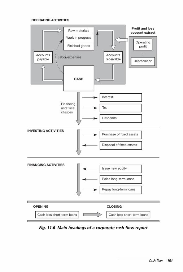
Cash flow 151Cash flow 151
Raw materials
Work in progress
Finished goods
Accountspayable
Accountsreceivable
CASH
Financingand fiscalcharges
OPERATING ACTIVITIES
Operatingprofit
Depreciation
Interest
Tax
Dividends
Purchase of fixed assets
Disposal of fixed assets
INVESTING ACTIVITIES
Issue new equity
Raise long-term loans
Repay long-term loans
FINANCING ACTIVITIES
OPENING
Cash less short-term loans
CLOSING
Profit and lossaccount extract
+
Cash less short-term loans
Labor/expenses
Fig. 11.6 Main headings of a corporate cash flow report
WKMR_CH11.QXD 11/24/05 12:21 PM Page 151

WKMR_CH11.QXD 11/24/05 12:21 PM Page 152
Part IV Determinants ofcorporate value
WKMR_CH12.QXD 11/24/05 12:22 PM Page 153

154 Key management ratios
WKMR_CH12.QXD 11/24/05 12:22 PM Page 154

12 CorporatevaluationIntroduction · Share values
He used to watch the market most precisely,and got in first, and so he did quite nicely.GEOFFREY CHAUCER (1380)
WKMR_CH12.QXD 11/24/05 12:22 PM Page 155
156 Key management ratios
Introduction
The value of public companies is determined by the stockmarket. Thevalue of companies not publicly quoted will be greatly influenced by thesame market. In this chapter, therefore, we will look at the main stock-market-related ratios.
These are:
■ market capitalization ■ share values, nominal, book, market ■ earnings per share (EPS) ■ dividends per share (DPS) ■ dividend cover and the pay-out ratio■ earnings yield ■ dividend yield ■ price to earnings ratio (PE) ■ market to book ratio.
In figure 12.1 we again see the balance sheet for the Example Co. plc. Thetop right-hand box shows common or owners’ funds totaling $360. Variousaccounting rules have been applied over many years in arriving at this value,e.g., how much depreciation has been charged to the profit/loss account?
A more pragmatic approach to determine the value of owners’ funds isto take the total assets figure of $800 and deduct from it the total loansfigure of $440 (200 + 240). This approach gives us the same answer in ourexample but it emphasizes the importance of the asset values in deter-mining shareholders’ funds. The authentic value for owners’ funds isderived simply by taking the total value of all assets in todays’ terms anddeducting all third party liabilities.
Some adjustments to assets values (and, possibly, liabilities) will proba-bly be necessary.
The more likely areas for adjustment are shown in figure 12.1, i.e.:
■ fixed assets■ inventories ■ certain liabilities.
✓
When we talk about the value of a company we mean its market capitalization orthe combined value of the common stock. We have already looked at the posi-tion that common shares occupy in the balance sheet and have seen where theystand in the queue for participation in profits. Both these issues are important foran understanding of this chapter.
?
%
WKMR_CH12.QXD 11/24/05 12:22 PM Page 156
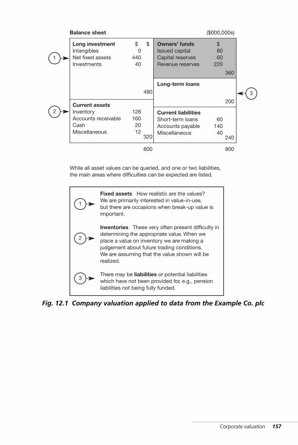
Corporate valuation 157
Long investmentIntangiblesNet fixed assetsInvestments
Current assetsInventoryAccounts receivableCashMiscellaneous
Owners’ fundsIssued capitalCapital reservesRevenue reserves
Long-term loans
Current liabilitiesShort-term loansAccounts payableMiscellaneous
8060
220
$
360
200
6014040
240
800
044040
$
480
$
1281602012
320
800
Balance sheet ($000,000s)
1
2
3
While all asset values can be queried, and one or two liabilities,the main areas where difficulties can be expected are listed.
Fixed assets How realistic are the values?We are primarily interested in value-in-use,but there are occasions when break-up value isimportant.
Inventories These very often present difficulty indetermining the appropriate value. When weplace a value on inventory we are making ajudgement about future trading conditions.We are assuming that the value shown will berealized.
There may be liabilities or potential liabilitieswhich have not been provided for, e.g., pensionliabilities not being fully funded.
1
2
3
Fig. 12.1 Company valuation applied to data from the Example Co. plc
WKMR_CH12.QXD 11/24/05 12:22 PM Page 157
158 Key management ratios
Share values
In chapter 2, three types of share value were mentioned. We now look atthese in detail using figures from the Example Co. plc (figure 12.2). Thereare 32 million issued common shares, for each of which there is a:
Nominal (par) value of $2.50Book (asset) value of $11.25 Market value of $22.50.
Let us now look at each of these in turn.
Nominal (par) value $2.50
Book value (asset value, or asset backing) $11.25
This value is arrived at by dividing the number of issued shares – 32m – into theowners’ funds of $360m. The book value of all the shares is $360m. Thereforeeach share has a book value of $11.25. You will recall that we discussed the needto validate that sum of $360m. For instance, if an examination of the inventoriesproduced a more prudent valuation of $20m less than the balance sheet value($108m), this write-down would reduce the common funds from 360m to 340m.The book value would fall from $11.25 to $10.62 per share.
?
The nominal value is largely a notional low figure arbitrarily placed on a com-pany’s stock. It serves to determine the value of ‘issued common stock’, i.e., inthe Example Co. the number of issued shares is 32m. The par value is $2.5 togive a value of $80m. If new shares are issued, they will hold this same nominalvalue even though the issue price will be much above it, probably close to thecurrent market price. Say new shares go out at a price of $17.50, there is a sur-plus of $15.00 over the nominal value. This surplus is called the ‘share premium’and it forms part of the capital reserves. Many companies have shares of ‘no parvalue’. They simply put it in the books at the price they were sold at.
?
WKMR_CH12.QXD 11/24/05 12:22 PM Page 158
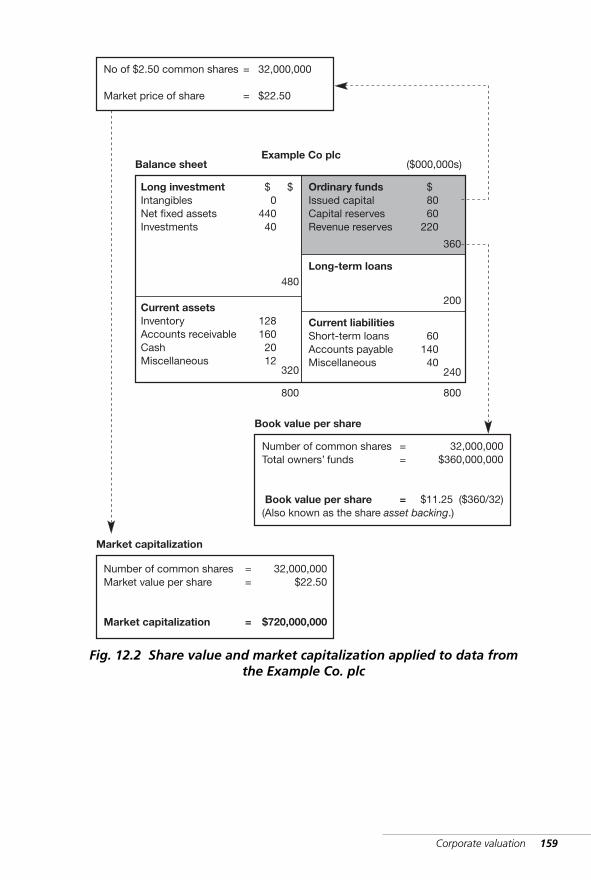
Corporate valuation 159
32,000,000$360,000,000
$11.25 ($360/32)
Number of common sharesTotal owners’ funds
Book value per share(Also known as the share asset backing.)
==
=
No of $2.50 common shares
Market price of share
=
=
32,000,000
$22.50
Book value per share
Long investmentIntangiblesNet fixed assetsInvestments
Current assetsInventoryAccounts receivableCashMiscellaneous
Ordinary fundsIssued capitalCapital reservesRevenue reserves
Long-term loans
Current liabilitiesShort-term loansAccounts payableMiscellaneous
8060
220
$
360
200
6014040
240
800
044040
$
480
$
1281602012
320
800
Balance sheet ($000,000s)Example Co plc
32,000,000$22.50
$720,000,000
Number of common sharesMarket value per share
Market capitalization
==
=
Market capitalization
Fig. 12.2 Share value and market capitalization applied to data fromthe Example Co. plc
WKMR_CH12.QXD 11/24/05 12:22 PM Page 159
160 Key management ratios
Market value $22.50
These different values will be used to derive the various ratios explored inthe rest of the chapter.
Earnings per share (EPS)
‘Earnings per share’ is one of the most widely quoted statistics whenthere is a discussion of a company’s performance or share value.
Figure 12.3 shows how this ratio is calculated. Remember that thecommon shareholder comes last in the queue for participating in profit.The profit used in the calculation is the figure after all other claimantshave been satisfied. The most common prior charges in the profit and lossaccount are interest and tax.
Therefore it is the earnings after tax (EAT) figure that is divided by thenumber of common shares to calculate the value of earnings per share.This figure tells us what profit has been earned by the common share-holder for every share held.
It serves no purpose to compare the earnings per share in one companywith that in another because a company can elect to have a large numberof shares of low denomination or a smaller number of a higher denomina-tion. A company can also decide to increase or reduce the number ofshares on issue. This decision will automatically alter the earnings pershare. We cannot say, therefore, that a company with an earnings pershare value of 50¢ is any better than one with a value of 40¢.
While the absolute amount of earnings per share tells nothing about acompany’s performance, the growth in EPS over time is a very importantstatistic. Indeed, many chairpersons stress it as a prime target in annualreports. Furthermore, growth in earnings per share has a significantinfluence on the market price of the share.
This is the price quoted in the Stock Exchange for a public company or an esti-mated price for a non-quoted company. On the Stock Exchange the figurechanges daily in response to actual or anticipated results and overall or sectoralsentiment of the market as reflected in the Stock Exchange indices. It is sug-gested that the main objective of management is to secure the best price possibleunder any set of conditions.
?
%
WKMR_CH12.QXD 11/24/05 12:22 PM Page 160
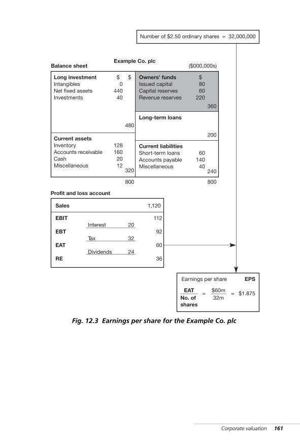
Corporate valuation 161
Number of $2.50 ordinary shares = 32,000,000
Long investmentIntangiblesNet fixed assetsInvestments
Current assetsInventoryAccounts receivableCashMiscellaneous
Owners’ fundsIssued capitalCapital reservesRevenue reserves
Long-term loans
Current liabilitiesShort-term loansAccounts payableMiscellaneous
8060
220
$
360
200
6014040
240
800
044040
$
480
$
1281602012
320
800
Balance sheet ($000,000s)Example Co. plc
Sales
Profit and loss account
1,120
EBIT
EBT
EAT
RE
Interest
Tax
Dividends
20
32
24
112
92
60
36
Earnings per share
$60m32m
= $1.875EATNo. ofshares
=
EPS
Fig. 12.3 Earnings per share for the Example Co. plc
WKMR_CH12.QXD 11/24/05 12:22 PM Page 161
162 Key management ratios
Growth in EPS tells us more about a company’s progress than growth inabsolute profits. Growth in profits can result from a great many things.For instance, a company could acquire another for shares and therebyincrease its profit. However, if the percentage increase in profit is lessthan the percentage increase in the number of shares, earnings per sharewill fall even with higher profits.
Not only is growth in EPS most important, so also is its stability.Investors look closely at the quality of earnings. They dislike the erraticperformance of companies with widely fluctuating profits. A high-qualityrating is given to earnings that are showing steady, non-volatile growth.
Dividends per share (DPS)
Figure 12.4 shows how to calculate this value. Only a fraction of the earn-ings accruing to the shareholders is paid out to them in cash. Theremainder is retained to consolidate and expand the business.
It is a well-established rule that dividends are paid only out of profits, notfrom any other source. However, the earnings need not necessarily fallinto the same year as the dividends. Therefore situations can arise whendividends exceed earnings. In such cases, dividends are being paid fromearnings that have been retained in the business from previous years.
The total return to the shareholder over any given time consists of thedividend received plus the growth in the share price. While for someinvestors growth is most important, many shareholders and potentialinvestors – both private individuals and institutions such as pensionfunds who need income for their day-to-day affairs – pay very close atten-tion to dividends. They look at the absolute dividend per share and for ahistory of stable but growing payments.
Therefore companies dislike intensely to have to reduce the dividendbecause this will drive away investors with possibly serious effects onshare price. A company in a difficult year will often decide that it must paya dividend in excess of earnings rather than cut the pay-out. Of course,this policy can be followed only for a short time and when there is reasonto believe that earnings will recover to a figure greater than the dividends.
%
☛
WKMR_CH12.QXD 11/24/05 12:22 PM Page 162
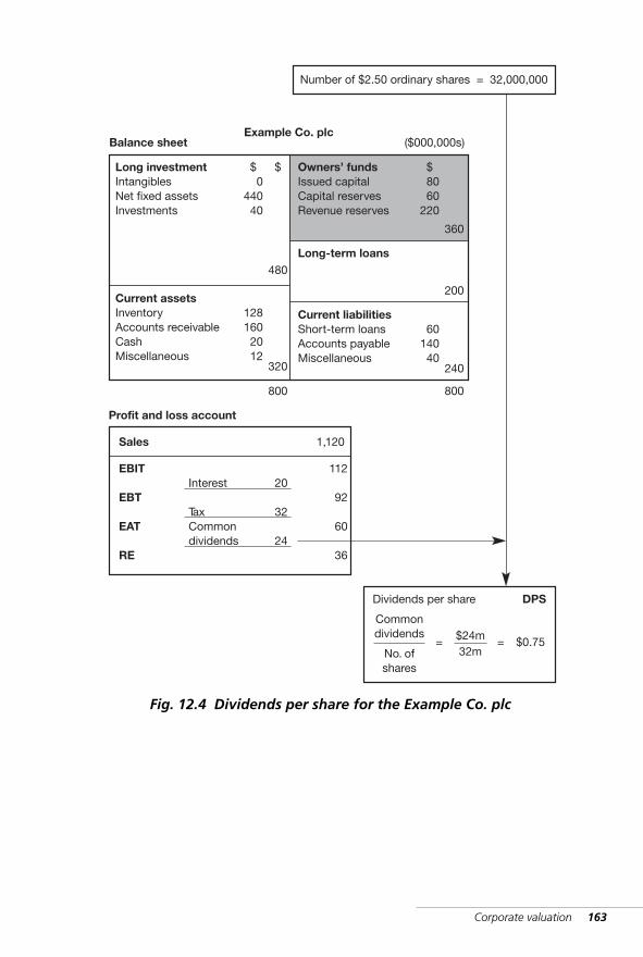
Corporate valuation 163
Number of $2.50 ordinary shares = 32,000,000
Long investmentIntangiblesNet fixed assetsInvestments
Current assetsInventoryAccounts receivableCashMiscellaneous
Owners’ fundsIssued capitalCapital reservesRevenue reserves
Long-term loans
Current liabilitiesShort-term loansAccounts payableMiscellaneous
8060
220
$
360
200
6014040
240
800
044040
$
480
$
1281602012
320
800
Balance sheet ($000,000s)Example Co. plc
Sales
Profit and loss account
1,120
EBIT
EBT
EAT
RE
Interest
TaxCommondividends
20
32
24
112
92
60
36
Dividends per share
$24m32m
= $0.75
Commondividends
No. ofshares
=
DPS
Fig. 12.4 Dividends per share for the Example Co. plc
WKMR_CH12.QXD 11/24/05 12:22 PM Page 163
164 Key management ratios
Dividend cover and the pay-out ratio
These two ratios are mirror images of one another and give the same infor-mation. Both express the relationship between a company’s earnings andthe cash paid out in dividends. Figure 12.5 shows the calculations. For thefirst ratio divide EPS by DPS. For the second reverse the numbers.*
Companies adopt dividend policies to suit their business needs. These willreflect the sectors in which they operate and the specific strategies theyadopt. Fast-growing companies have a great need for cash and they payout little. On the other hand stable low-growth companies pay out a highpercentage of earnings.
We therefore see that public utility companies are noted for high stablepay-out policies. They are therefore, very popular with investors forwhom income is the most important consideration. On the other hand,some computer companies have never paid a dividend, even though theyhave made large profits over many years. These companies attractinvestors who look for capital growth.
The importance of the dividend cover is the indication it gives of thefuture stability and growth of the dividend:
■ a high cover (low pay-out ratio) suggests that the dividend is fairlysafe, because it can be maintained in the face of any expecteddownturn in profit
■ a high cover also indicates a high retention policy, which suggeststhat the company is aiming for high growth.
✓
* These calculations use the earnings and dividend for a single share to arrive at the results.We can also use the earnings and dividend for the total company to derive the same results,as has been done for the US Consolidated Company Inc. in figure 12.6.
%
WKMR_CH12.QXD 11/24/05 12:22 PM Page 164
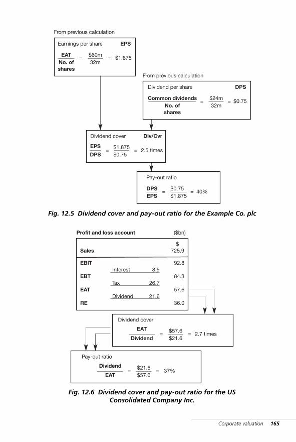
Corporate valuation 165
Earnings per share
$60m32m
= $1.875EATNo. ofshares
=
Dividend per share
$24m32m
= $0.75Common dividendsNo. ofshares
=
Dividend cover
$1.875$0.75
= 2.5 timesEPS
DPS=
Pay-out ratio
$0.75$1.875
= 40%DPSEPS
=
EPS
From previous calculation
DPS
Div/Cvr
From previous calculation
Fig. 12.5 Dividend cover and pay-out ratio for the Example Co. plc
Dividend cover
Pay-out ratio
Sales
Profit and loss account
725.9$
EBIT
EBT
EAT
RE
Interest
Tax
Dividend
8.5
26.7
21.6
92.8
84.3
57.6
36.0
($bn)
$57.6$21.6
= 2.7 timesEAT
Dividend=
$21.6$57.6
= 37%Dividend
EAT=
Fig. 12.6 Dividend cover and pay-out ratio for the US Consolidated Company Inc.
WKMR_CH12.QXD 11/24/05 12:22 PM Page 165
166 Key management ratios
Figures 12.6 and 12.7 show what level of cover is normal. In USConsolidated Inc., it is 2.7 times (equal to a 37 percent pay-out ratio).This tells us that in most companies more that 50 percent of availableprofit is ploughed back into the operation.
The country and sectoral analysis charts in figure 12.7 show how closelyinternational companies cluster around the average (Japan is the excep-tion with a dividend cover greater than 6 times). It is not surprising,given their high historic growth rates.
It is worthwhile considering the implication of these numbers.Companies in the main retain more profits than they distribute. More than50 percent of equity returns, therefore, should come from capital growth,not dividends. However, capital growth depends on the share price.
Most share prices show significant fluctuations around a central trendline. Therefore, the actual capital gain delivered to a particular investor isheavily dependent on the timing of the investment and its later conver-sion back into cash.
For instance, an investor in a high growth stock would suffer a capitalloss if he bought at the high and sold at the low point in the cycle.
%
%
WKMR_CH12.QXD 11/24/05 12:22 PM Page 166
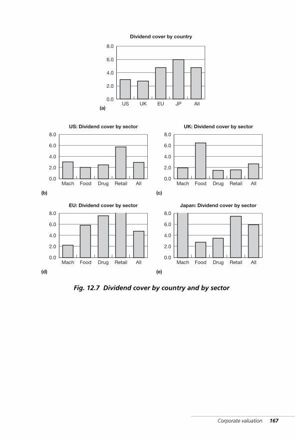
Corporate valuation 167
8.0
6.0
4.0
2.0
0.0
EU: Dividend cover by sector
(d)
Mach Food Drug Retail All
8.0
6.0
4.0
2.0
0.0
Japan: Dividend cover by sector
(e)
Mach Food Drug Retail All
8.0
2.0
0.0US
Dividend cover by country
(a)UK EU JP All
6.0
4.0
8.0
6.0
4.0
2.0
0.0
US: Dividend cover by sector
(b)
Mach Food Drug Retail All
8.0
6.0
4.0
2.0
0.0
UK: Dividend cover by sector
(c)
Mach Food Drug Retail All
Fig. 12.7 Dividend cover by country and by sector
WKMR_CH12.QXD 11/24/05 12:22 PM Page 167
168 Key management ratios
Earnings and dividend yield ratios
Figure 12.8 shows calculations for the Example Co. plc.The earnings yield shows the relationship that EPS bears to the share
price. For instance, if the EPS is $1.50 and the share price is $10.00 theearnings yield is 15 percent. If the share price moved up to $15.00 thecorresponding yield would be 10 percent. As the share price increases theyield falls. Paradoxically, a low yield indicates a share that is in muchdemand by investors. We will see in the next section its link to the priceearnings ratio.
From the company point of view, the ratio indicates the return the com-pany must provide to attract investors. If a company falls out of favor inthe market-place the share price falls and the company is faced with ahigher yield. It follows that a company with a poor image has to pay ahigh return to attract capital.
For the investor, yield calculations allow comparisons to be madebetween the return on shares and other types of investment, such as gov-ernment stocks (gilts) or commercial property.
Managers of large investment funds constantly balance their portfoliosbetween these different investment outlets. In doing so, they take accountof the relative yields which change daily, together with the stability andcapital growth expected in each area.
Whereas the earnings yield specifies the total return, the dividend yield ismore important for investors dependent on income from the shares. Itallows them to compare the cash flow that they will receive from invest-ing a fixed sum in different stocks or other investment outlets. As wehave seen in the previous section, public utility companies with high pay-out ratios tend to produce high dividend yields and would be popular withpension fund managers.
The degree of variation in yield values is shown in the country variationsillustrated in figure 12.8. The most striking result is the dividend yield forJapan at less than 1 percent. This is brought about by the low pay-outratio already mentioned and high share prices.
☛
The yield on a share expresses the return it provides in terms of earnings or divi-dends as a percentage of the current share price. Both measures are importantfor both the investor and the company.
?
WKMR_CH12.QXD 11/24/05 12:22 PM Page 168
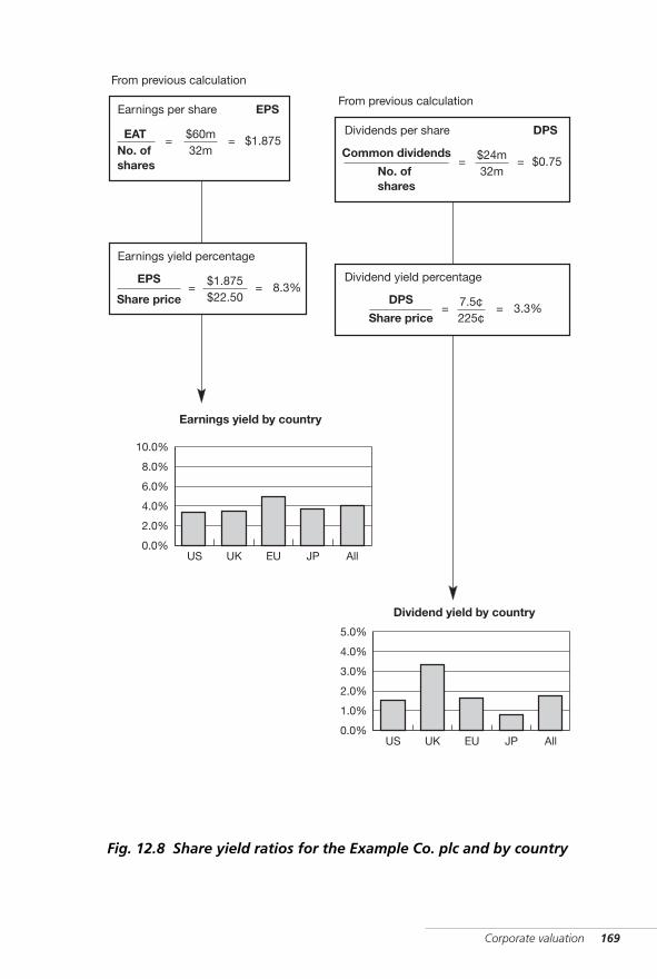
Corporate valuation 169
Earnings per share
$60m32m
= $1.875EATNo. ofshares
=Dividends per share
$24m32m
= $0.75Common dividends
No. ofshares
=
Earnings yield percentage
$1.875$22.50
= 8.3%EPS
Share price=
Dividend yield percentage
7.5¢225¢
= 3.3%DPS
Share price=
EPS
DPS
10.0%
6.0%
4.0%
2.0%
0.0%US
Earnings yield by country
UK EU JN All
8.0%
5.0%
3.0%
2.0%
1.0%
0.0%US
Dividend yield by country
UK EU JN All
4.0%
From previous calculation
From previous calculation
Fig. 12.8 Share yield ratios for the Example Co. plc and by country
10.0%
8.0%
4.0%
2.0%
0.0%US UK EU JP All
6.0%
5.0%
4.0%
2.0%
1.0%
0.0%US UK EU JP All
3.0%
WKMR_CH12.QXD 11/24/05 12:22 PM Page 169
170 Key management ratios
These yield values are low in comparison to gilt yields. The expression‘reverse yield gap’ is used to highlight the shortfall in dividend yields asopposed to those for gilts.
Price to earnings ratio (P/E)
While the calculation of the ratio is based on figures from the past, itsvalue is determined by investors whose focus is on the future. They areprimarily interested in the prospects for earnings growth. To estimatethis they will look to the industrial sector, the company’s products, itsmanagement and its financial stability and growth history.
The company has no direct control over the PE ratio. It may influenceit over the short-term by a good public relations exercise. In the long-term, however, it must deliver a good return to the equity shareholder tosecure a continued high rating.
The advantages of a high price to earnings ratio value are considerable.The wealth of the company’s owners is increased in proportion. Newfunds can be raised at a favorable price. The possibility of a successfulhostile takeover bid is much reduced. Most importantly, the company hasthe means to make acquisitions on favorable terms by using its ‘paper’(shares), as opposed to cash.
When we look at the P/E ratio across international boundaries (see figure12.9), we see that the US and the UK show similiar values just short of 30 times. The returns for the EU are considerably lower, but we notice a considerable jump when we come to Japan. Here the current value isapproximately 28, even though the market has fallen by 50 percent.
Japanese P/E values have puzzled western investors for years. A shortwhile ago, many companies were in the 50 to 60 range. Attempts toexplain this mentioned very low inflation rates, strong currency, low costof capital etc. However stockmarket prices fell sharply and rates, whilestill high, are now more in line with western world norms.
%
The price to earnings ratio or ‘multiple’ is a widely quoted parameter of sharevalue. Figure 12.9 shows the method of calculation. The share price is divided bythe EPS figure. The answer gives the number of years’ purchase that the pricebears to earnings.
?
☛
WKMR_CH12.QXD 11/24/05 12:22 PM Page 170
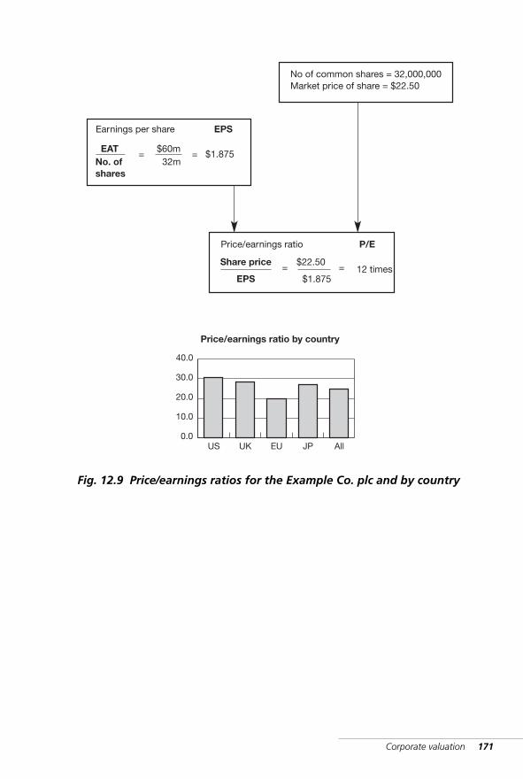
Corporate valuation 171
Price/earnings ratio by country
Earnings per share
$60m32m
= $1.875EATNo. ofshares
=
Price/earnings ratio
$1.875
$22.50= 12 times
EPS
Share price=
EPS
P/E
No of common shares = 32,000,000Market price of share = $22.50
40.0
30.0
20.0
10.0
0.0US UK EU JP All
Fig. 12.9 Price/earnings ratios for the Example Co. plc and by country
40.0
30.0
20.0
10.0
0.0US UK EU JP All
WKMR_CH12.QXD 11/24/05 12:22 PM Page 171
172 Key management ratios
Market to book ratio
Figure 12.10 shows the calculation. The ratio relates the total marketcapitalization of the company to the shareholders’ funds. To express it inanother way, it compares the value in the stockmarket with the share-holders’ investment in the company.
The answer will be less than, greater than or equal to unity. It is theinvestors’ perception of the performance of the company in terms of profits,balance sheet strength or liquidity and growth that determines this ratio.
A value of less than unity means that the shareholders’ investment hasdiminished in value; it has wasted away. The investing community havegiven a ‘thumbs down’ signal to the company. They do not anticipate thatfuture profits will be sufficient to justify the current owners’ investmentin the company.
On the other hand, when this value is well in excess of unity, it meansthat the investment has been multiplied by the market/book factor. A highratio does not simply mean that the worth of the company has increasedover time by means of its retained earnings. The multiplier acts in addi-tion to this. Each $1 of original investment, plus each $1 of retainedearnings is multiplied by a factor equal to the market to book ratio.
%
The market to book ratio gives the final and, perhaps the most thorough assess-ment by the stockmarket of a company’s overall status. It summarizes theinvestors’ view of the company overall, its management, its profits, its liquidity,and future prospects.
?
WKMR_CH12.QXD 11/24/05 12:22 PM Page 172
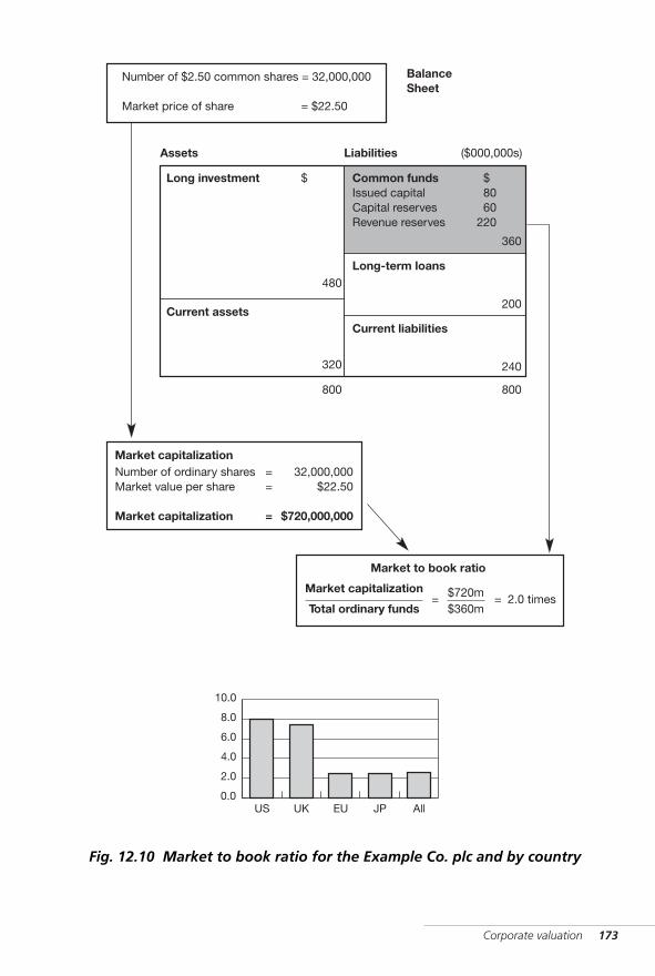
Corporate valuation 173
Market to book ratio
$720m$360m
= 2.0 timesMarket capitalization
Total ordinary funds=
Number of $2.50 common shares = 32,000,000
Market price of share = $22.50
Number of ordinary sharesMarket value per share
Market capitalization
==
=
32,000,000$22.50
$720,000,000
Market capitalization
Long investment
Current assets
Common fundsIssued capitalCapital reservesRevenue reserves
Long-term loans
Current liabilities
8060
220
$
360
200
240
800
$
480
320
800
Assets ($000,000s)
10.00
8.00
6.00
2.00
0.00US UK EU JN All
Liabilities
BalanceSheet
4.00
Fig. 12.10 Market to book ratio for the Example Co. plc and by country
10.0
6.0
4.0
2.0
0.0US UK EU JP All
8.0
WKMR_CH12.QXD 11/24/05 12:22 PM Page 173
Two important questions must be kept in mind when considering this ratio:
■ Do the shareholders’ funds reflect a realistic value for the assets? ■ Is the market rating going through an exceptionally high or low
phase?
Refer to appendix 1 for various items that can affect this ratio.The country analysis in figure 12.10 shows widely differing values
between the US and UK on the one hand and the rest of the EU andJapan on the other. In normal circumstances we would expect a value ofbetween 2 and 3 times for this ratio, and these are the values we see forthe EU and Japan. The extraordinary high values we encounter in the USand UK can only be accounted for by:
■ the extraordinary exuberance in the market at the time;
■ the understatement of owners’ equity as a result of goodwill write-downs.
The fall in the overall market will have reduced the numbers considerably.The absolute minimum that management must achieve for this ratio is
1.0. Good companies produce a factor of 2.0.
174 Key management ratios
✓
WKMR_CH12.QXD 11/24/05 12:22 PM Page 174
13 Financialleverage and corporate valuation Introduction · Financial leverage
· V chart · Market to book ratio
Auditors are the troops who watch battlefrom the safety of a hillside and when thebattle is over come down to count the deadand bayonet the wounded.ANONYMOUS
WKMR_CH13.QXD 11/24/05 12:22 PM Page 175
176 Key management ratios
Introduction
This chapter will integrate material from previous chapters into onesingle web supporting corporate value and it will show the relationshipsthat exist between many of the ratios covered so far. Specifically it will:
1. establish the financial leverage links between ROTA and ROE
2. examine further the great importance of ROE
3. tie together – operating efficiency measures
– leverage ratios
– valuation factors
so as to identify and quantify the drivers of corporate value.To accomplish this we will make much use of the V chart (valuation chart).
Financial leverage
The material that follows will give some appreciation of this.The concept of leverage, or gearing, was looked at briefly in chapter 10.
It was seen that high leverage could substantially increase the return tothe shareholder. This chapter will explore further the impact of leverageand the specific elements that link ROTA and ROE.
We have seen in chapter 6, figure 6.3, that the US Consolidated CompanyInc. showed the following values:
■ ROTA 13.3%■ ROE 19.6%
Financial mechanisms have been used to transform a pretax return of13.3 percent from the total company into an after-tax return of 19.6 per-cent to the shareholders. This is leverage in action. The financialvariables that link these two values are laid out diagrammatically infigure 13.1, viz:
debt to equity ratio 1.8 timesaverage interest cost 3.3%tax rate 38%
The term ‘financial engineering’ has become quite popular. It is used in relation toschemes that increase the return to the shareholders from a given return earnedby the company.
✓
!
%
WKMR_CH13.QXD 11/24/05 12:22 PM Page 176
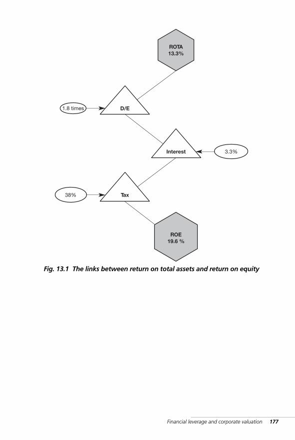
Financial leverage and corporate valuation 177
ROTA13.3%
D/E1.8 times
Interest 3.3%
Tax38%
ROE19.6 %
Fig. 13.1 The links between return on total assets and return on equity
WKMR_CH13.QXD 11/24/05 12:22 PM Page 177
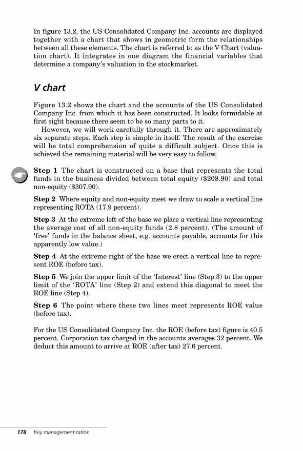
178 Key management ratios
In figure 13.2, the US Consolidated Company Inc. accounts are displayedtogether with a chart that shows in geometric form the relationshipsbetween all these elements. The chart is referred to as the V Chart (valua-tion chart). It integrates in one diagram the financial variables thatdetermine a company’s valuation in the stockmarket.
V chart
Figure 13.2 shows the chart and the accounts of the US ConsolidatedCompany Inc. from which it has been constructed. It looks formidable atfirst sight because there seem to be so many parts to it.
However, we will work carefully through it. There are approximatelysix separate steps. Each step is simple in itself. The result of the exercisewill be total comprehension of quite a difficult subject. Once this isachieved the remaining material will be very easy to follow.
Step 1 The chart is constructed on a base that represents the totalfunds in the business divided between total equity ($208.90) and totalnon-equity ($307.90).
Step 2 Where equity and non-equity meet we draw to scale a vertical linerepresenting ROTA (17.9 percent).
Step 3 At the extreme left of the base we place a vertical line representingthe average cost of all non-equity funds (2.8 percent). (The amount of‘free’ funds in the balance sheet, e.g. accounts payable, accounts for thisapparently low value.)
Step 4 At the extreme right of the base we erect a vertical line to repre-sent ROE (before tax).
Step 5 We join the upper limit of the ‘Interest’ line (Step 3) to the upperlimit of the ‘ROTA’ line (Step 2) and extend this diagonal to meet theROE line (Step 4).
Step 6 The point where these two lines meet represents ROE value(before tax).
For the US Consolidated Company Inc. the ROE (before tax) figure is 40.5percent. Corporation tax charged in the accounts averages 32 percent. Wededuct this amount to arrive at ROE (after tax) 27.6 percent.
☛
WKMR_CH13.QXD 11/24/05 12:22 PM Page 178
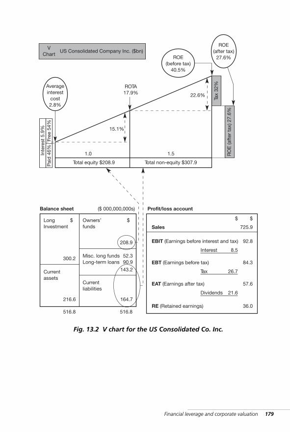
Financial leverage and corporate valuation 179
LongInvestment
Balance sheet
22.6%
15.1%
RO
E (a
fter
tax
) 27.
6%
Tax
32%
Pai
d 4
6%Fr
ee 5
4%In
tere
st 5
.9%
Total non-equity $307.9
1.5
Total equity $208.9
1.0
Averageinterest
cost2.8%
ROTA17.9%
ROE(before tax)
40.5%
($ 000,000,000s)
ROE(after tax)
27.6%
VChart
US Consolidated Company Inc. ($bn)
Currentassets
Currentliabilities
Misc. long fundsLong-term loans
Owners’funds
$ $
300.2
208.9
216.6
52.390.9
143.2
164.7
516.8 516.8
Profit/loss account
Sales
EBIT (Earnings before interest and tax)
Interest 8.5
92.8
EBT (Earnings before tax)
Tax 26.7
84.3
EAT (Earnings after tax)
21.6
57.6
RE (Retained earnings) 36.0
725.9
$
Dividends
$
Fig. 13.2 V chart for the US Consolidated Co. Inc.
WKMR_CH13.QXD 11/24/05 12:22 PM Page 179
180 Key management ratios
V chart dynamics
To understand the dynamics of financial leverage, we can look on theupper diagonal of the chart as a cantilevered beam that is anchored atits left extremity to the ‘Interest’ vertical. It is pushed upwards by theROTA piston.
The point of intersection with the ROE (before tax) line is determinedby three factors:
1. its ‘anchor’, i.e., average interest cost
2. ROTA value
3. the relative values for ‘equity’ and ‘non-equity’.
We can write this in an equation:
ROE (pre-tax) = ROTA + [(ROTA – Interest) × D/E]40.5% = 17.9% + [(17.9% – 2.8%) × 1.5]
We can use either the chart or the formula to track a change in any of theinput values to its effect on ROE (before tax). By allowing for tax, we canget to ROE (after tax).
Three examples are shown in figure 13.3.
Example A. Increase ROTA by 1% to 18.9%.Answer: ROE (before tax) = 43%
Example B. Increase non-equity/equity to 2.0 timesAnswer: ROE (before tax) = 48%
Example C. Increase interest cost by 0.5%Answer: ROE (before tax) = 39.8%
We have identified and quantified the variables that link the ROTA toROE. It only remains to link ROE to company value. When this is com-plete we will be able to trace a path from the shop-floor variables rightthrough to stock-market value. This will be addressed in the next section.
%
%
WKMR_CH13.QXD 11/24/05 12:22 PM Page 180
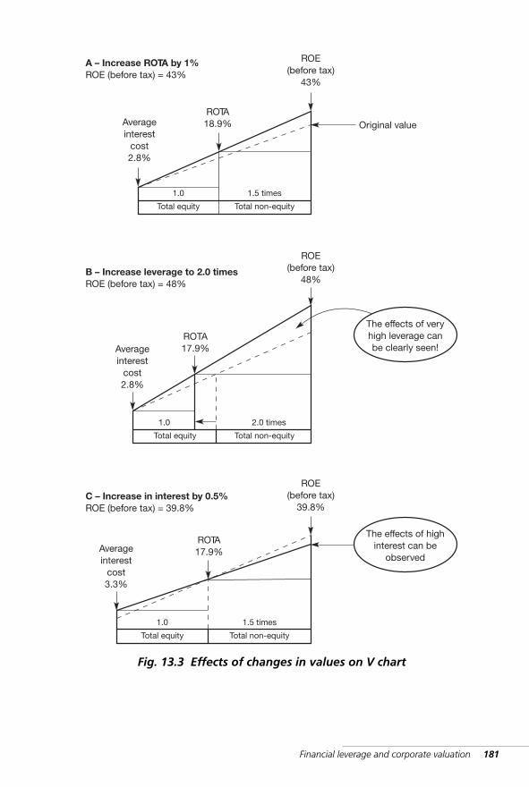
Financial leverage and corporate valuation 181
Total non-equity
1.5 times
Total equity
1.0
Averageinterest
cost2.8%
ROTA18.9%
ROE(before tax)
43%
Total non-equity
2.0 times
Total equity
1.0
Averageinterest
cost2.8%
ROTA17.9%
ROE(before tax)
48%
Total non-equity
1.5 times
Total equity
1.0
Averageinterest
cost3.3%
ROTA17.9%
ROE(before tax)
39.8%
A – Increase ROTA by 1%ROE (before tax) = 43%
B – Increase leverage to 2.0 timesROE (before tax) = 48%
The effects of veryhigh leverage canbe clearly seen!
C – Increase in interest by 0.5%ROE (before tax) = 39.8%
The effects of highinterest can be
observed
Original value
Fig. 13.3 Effects of changes in values on V chart
WKMR_CH13.QXD 11/24/05 12:22 PM Page 181
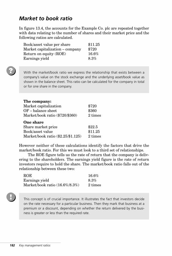
182 Key management ratios
Market to book ratio
In figure 13.4, the accounts for the Example Co. plc are repeated togetherwith data relating to the number of shares and their market price and thefollowing ratios are calculated.
Book/asset value per share $11.25Market capitalization – company $720Return on equity (ROE) 16.6%Earnings yield 8.3%
The company:Market capitalization $720OF – balance sheet $360Market/book ratio ($720/$360) 2 times
One shareShare market price $22.5Book/asset value $11.25Market/book ratio ($2.25/$1.125) 2 times
However neither of these calculations identify the factors that drive themarket/book ratio. For this we must look to a third set of relationships.
The ROE figure tells us the rate of return that the company is deliv-ering to the shareholders. The earnings yield figure is the rate of returninvestors require to hold the share. The market/book ratio falls out of therelationship between these two:
ROE 16.6%Earnings yield 8.3%Market/book ratio (16.6%/8.3%) 2 times
This concept is of crucial importance. It illustrates the fact that investors decideon the rate necessary for a particular business. Then they mark that business at apremium or a discount, depending on whether the return delivered by the busi-ness is greater or less than the required rate.
!
With the market/book ratio we express the relationship that exists between acompany’s value on the stock exchange and the underlying asset/book value asshown in the balance sheet. This ratio can be calculated for the company in totalor for one share in the company.
?
WKMR_CH13.QXD 11/24/05 12:22 PM Page 182
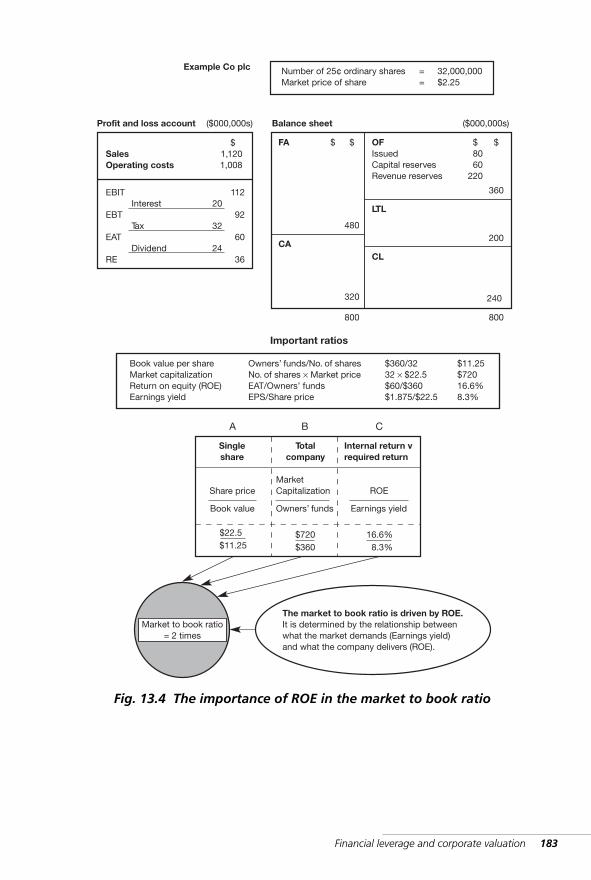
Financial leverage and corporate valuation 183
Book value per shareMarket capitalizationReturn on equity (ROE)Earnings yield
Owners’ funds/No. of sharesNo. of shares × Market priceEAT/Owners’ fundsEPS/Share price
$360/3232 × $22.5$60/$360$1.875/$22.5
$11.25$72016.6%8.3%
Totalcompany
MarketCapitalization
Owners’ funds
Singleshare
Share price
Book value
Internal return vrequired return
ROE
Earnings yield
$720$360
$22.5$11.25
16.6%8.3%
Market to book ratio= 2 times
The market to book ratio is driven by ROE.It is determined by the relationship betweenwhat the market demands (Earnings yield)and what the company delivers (ROE).
SalesOperating costs
Profit and loss account
1,1201,008
$
EBIT
EBT
EAT
RE
Interest
Tax
Dividend
20
32
24
112
92
60
36
FA
CA
OFIssuedCapital reservesRevenue reserves
LTL
CL
8060
220
$
360
$
200
240
800
$
480
$
320
800
Balance sheet ($000,000s)
A B C
Important ratios
($000,000s)
Example Co plc Number of 25¢ ordinary sharesMarket price of share
==
32,000,000$2.25
Fig. 13.4 The importance of ROE in the market to book ratio
WKMR_CH13.QXD 11/24/05 12:22 PM Page 183
184 Key management ratios
Importance of ROE
We have identified the drivers of ROE in the previous section. The mostimportant are ROTA and the debt/equity ratio. The factors that driveROTA are ‘margin’ and ‘turn’ (sales/total assets ratio) as we saw in chap-ter 7. Standing behind the ‘margin’ and ‘turn’ are all the operating ratios.So it is ROE that brings together all the operating and financing charac-teristics of the business.
We therfore can trace a path from the shop floor to stockmarket value.However we need to examine a little more the factors that help
the stockmarket decide on the earnings yield it will demand from a partic-ular company.
Figure 13.5 lists the main influencing factors under the headings:
■ Company■ Industry■ Economy.
Investors are buying the expected future returns of the company. Ifgrowth prospects are good this will promise high returns. However theytrade off risk against return. For a high perceived risk they will look for ahigh return.
So they weigh up the prospects for:
■ The economy overall■ The industrial sector■ The particular company.
The main items for consideration under each heading are shown infigure 13.5.
☛
ROE drives company value. There are those who will dispute this statement.With good logic they will argue this is too simple an explanation because ROE is ashort-term accounting measure. It does not take into account future growthprospects, etc. Nevertheless we can say that, other things being equal, the mostimportant driver of value is ROE.
!
WKMR_CH13.QXD 11/24/05 12:22 PM Page 184
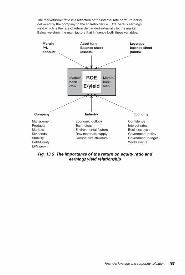
Financial leverage and corporate valuation 185
The market/book ratio is a reflection of the internal rate of return beingdelivered by the company to the shareholder i.e., ROE versus earningsyield which is the rate of return demanded externally by the market.Below we show the main factors that influence both these variables.
Asset turnBalance sheet(assets)
Leveragebalance sheet(funds)
MarginP/Laccount
ROE
E/yield
Market/bookratio
Industry EconomyCompany
Economic outlookTechnologyEnvironmental factorsRaw materials supplyCompetitive structure
ConfidenceInterest ratesBusiness cycleGovernment policyGovernment budgetWorld events
ManagementProductsMarketsDividendsStabilityDebt/EquityEPS growth
Market/bookratio
Fig. 13.5 The importance of the return on equity ratio andearnings yield relationship
WKMR_CH13.QXD 11/24/05 12:22 PM Page 185
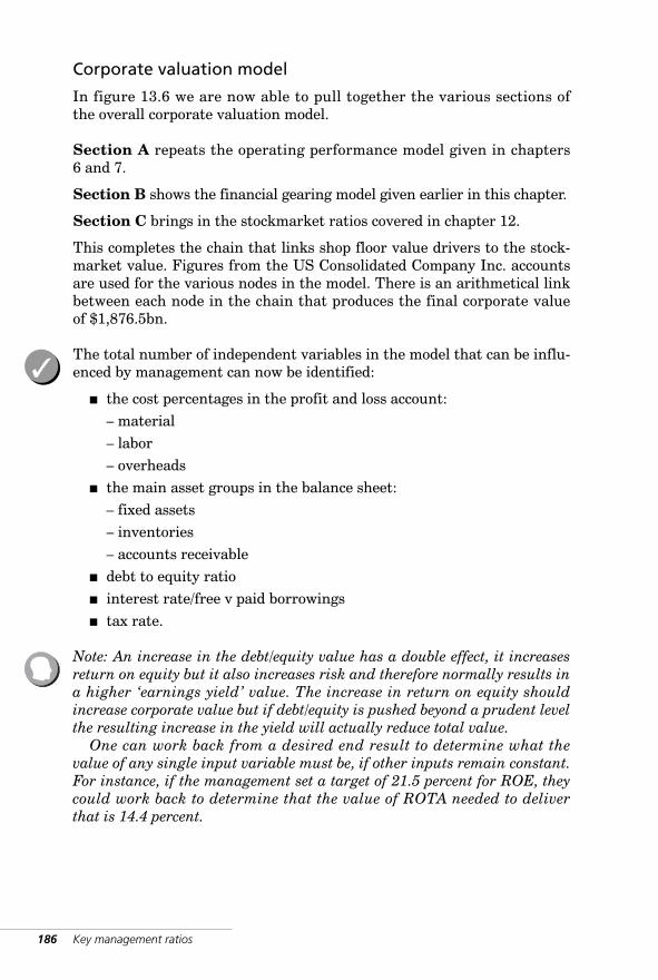
Corporate valuation model
In figure 13.6 we are now able to pull together the various sections ofthe overall corporate valuation model.
Section A repeats the operating performance model given in chapters6 and 7.
Section B shows the financial gearing model given earlier in this chapter.
Section C brings in the stockmarket ratios covered in chapter 12.
This completes the chain that links shop floor value drivers to the stock-market value. Figures from the US Consolidated Company Inc. accountsare used for the various nodes in the model. There is an arithmetical linkbetween each node in the chain that produces the final corporate valueof $1,876.5bn.
The total number of independent variables in the model that can be influ-enced by management can now be identified:
■ the cost percentages in the profit and loss account:– material– labor – overheads
■ the main asset groups in the balance sheet:– fixed assets – inventories – accounts receivable
■ debt to equity ratio ■ interest rate/free v paid borrowings ■ tax rate.
Note: An increase in the debt/equity value has a double effect, it increasesreturn on equity but it also increases risk and therefore normally results ina higher ‘earnings yield’ value. The increase in return on equity shouldincrease corporate value but if debt/equity is pushed beyond a prudent levelthe resulting increase in the yield will actually reduce total value.
One can work back from a desired end result to determine what thevalue of any single input variable must be, if other inputs remain constant.For instance, if the management set a target of 21.5 percent for ROE, theycould work back to determine that the value of ROTA needed to deliverthat is 14.4 percent.
186 Key management ratios
✓
WKMR_CH13.QXD 11/24/05 12:22 PM Page 186
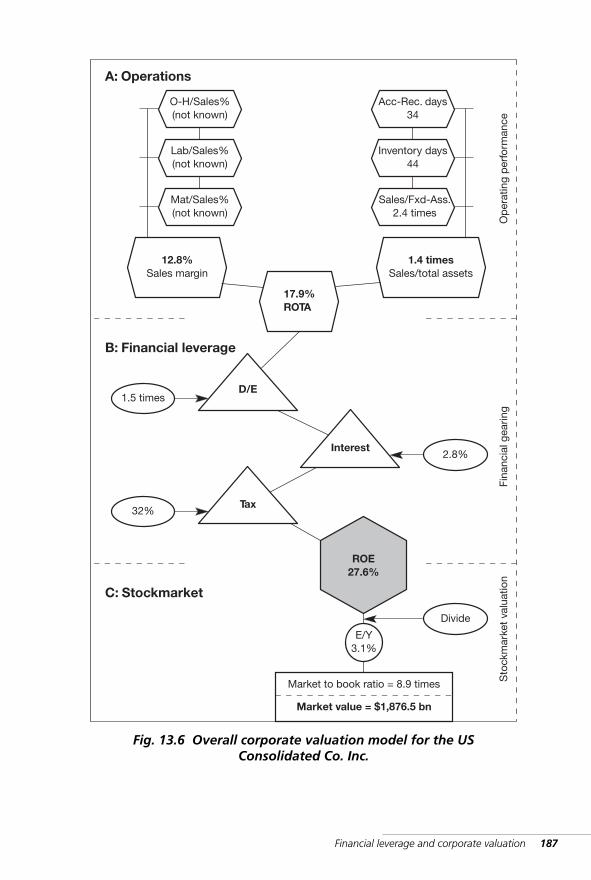
Financial leverage and corporate valuation 187
D/E1.5 times
Interest2.8%
Tax32%
ROE27.6%
17.9%ROTA
12.8%Sales margin
O-H/Sales%(not known)
1.4 timesSales/total assets
Lab/Sales%(not known)
Mat/Sales%(not known)
Acc-Rec. days34
Inventory days44
Sales/Fxd-Ass.2.4 times
E/Y3.1%
Market to book ratio = 8.9 times
Market value = $1,876.5 bn
A: Operations
B: Financial leverage
C: Stockmarket
Sto
ckm
arke
t va
luat
ion
Fina
ncia
l gea
ring
Op
erat
ing
per
form
ance
Divide
Fig. 13.6 Overall corporate valuation model for the USConsolidated Co. Inc.
WKMR_CH13.QXD 11/24/05 12:22 PM Page 187

WKMR_CH13.QXD 11/24/05 12:22 PM Page 188
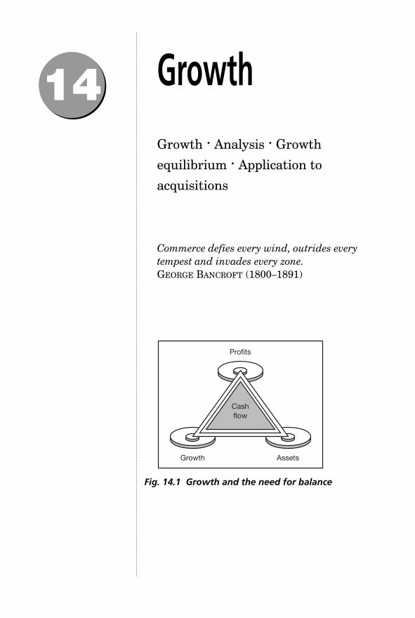
GrowthGrowth · Analysis · Growth
equilibrium · Application to
acquisitions
Growth Assets
Profits
Cashflow
14
Commerce defies every wind, outrides everytempest and invades every zone.GEORGE BANCROFT (1800–1891)
Fig. 14.1 Growth and the need for balance
WKMR_CH14.QXD 11/24/05 12:40 PM Page 189
190 Key management ratios
Growth
To assist in our analysis, we will take the case of the CABCO Constructioncompany shown in figure 14.2. This is a company that is suffering fromsevere problems of growth.
We see that it has been growing, in terms of sales, at approximately 15percent per annum. However, it has a rapidly deteriorating financial posi-tion. The current ratio has dropped from 2.3 to 1.4 times over the fouryears and the debt to total assets ratio has risen from 37 percent to 61percent over the same period. The liquidity ratios were very strong in1997 but have sunk to their lowest acceptable level by 2001. The mostworrying aspect of the case is the speed at which the liquidity positionhas deteriorated.
Performance, as measured by return on equity, was low but improvedsignificantly in 2001. It made a passable return of almost 20 percentbefore tax to its shareholders, but it is now close to a liquidity crisis.Accordingly, management must take urgent action to stop the downwardtrend and change the direction in which the company is going.
This chapter is concerned with the problem of identifying and quantify-ing the options open to management, but, more importantly, it will extractgeneral rules relating to company growth and how it can be handled.
Growth to a company is like medicine is to a patient – beneficial up to a certainlevel, but dangerous and possibly fatal when that level is exceeded. There is aneed for balance between profits, assets and growth (see figure 14.1). Anyimbalance between these factors will impact strongly on cash flow. Given theopportunities and corresponding dangers of growth, particularly in times of highinflation, it is wise to consider whether there is some way in which we can specifyfor a company what level of growth it can safely absorb. This chapter illustratesone particular method that many companies have found useful.
!
%
WKMR_CH14.QXD 11/24/05 12:40 PM Page 190
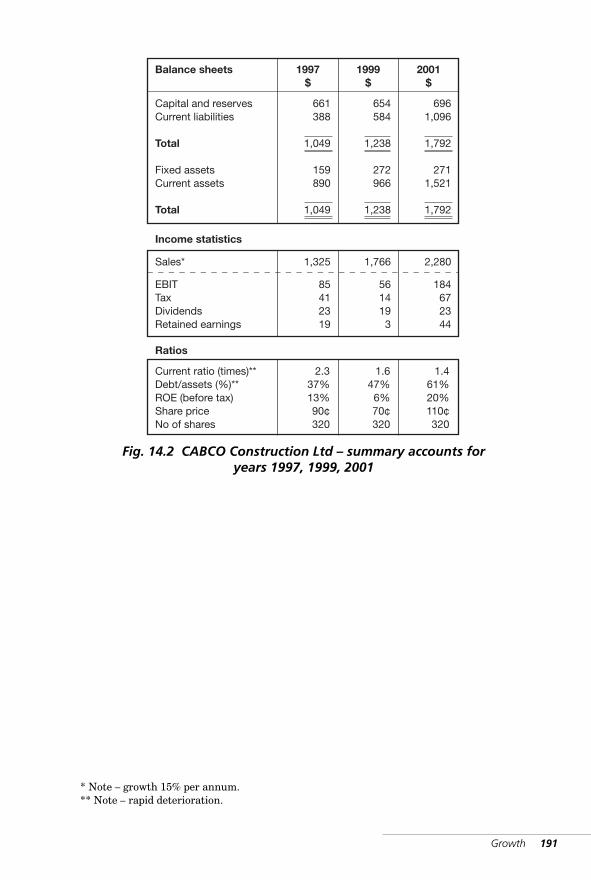
Growth 191
Balance sheets
Capital and reservesCurrent liabilities
Total
Fixed assetsCurrent assets
Total
Income statistics
Sales*
EBITTaxDividendsRetained earnings
Ratios
Current ratio (times)**Debt/assets (%)**ROE (before tax)Share priceNo of shares
1997$
661388
1,049
159890
1,049
85412319
2.337%13%90¢320
1,325
654584
1,238
272966
1,238
5614193
1.647%6%70¢320
1,766
6961,096
1,792
2711,521
1,792
184672344
1.461%20%110¢320
2,280
1999$
2001$
Fig. 14.2 CABCO Construction Ltd – summary accounts foryears 1997, 1999, 2001
* Note – growth 15% per annum.** Note – rapid deterioration.
WKMR_CH14.QXD 11/24/05 12:40 PM Page 191
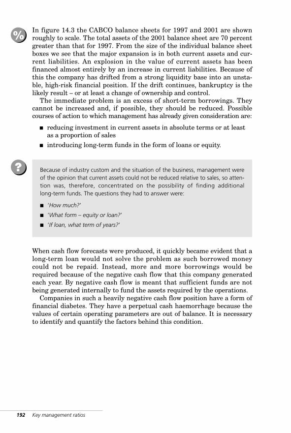
192 Key management ratios
In figure 14.3 the CABCO balance sheets for 1997 and 2001 are shownroughly to scale. The total assets of the 2001 balance sheet are 70 percentgreater than that for 1997. From the size of the individual balance sheetboxes we see that the major expansion is in both current assets and cur-rent liabilities. An explosion in the value of current assets has beenfinanced almost entirely by an increase in current liabilities. Because ofthis the company has drifted from a strong liquidity base into an unsta-ble, high-risk financial position. If the drift continues, bankruptcy is thelikely result – or at least a change of ownership and control.
The immediate problem is an excess of short-term borrowings. Theycannot be increased and, if possible, they should be reduced. Possiblecourses of action to which management has already given consideration are:
■ reducing investment in current assets in absolute terms or at leastas a proportion of sales
■ introducing long-term funds in the form of loans or equity.
When cash flow forecasts were produced, it quickly became evident that along-term loan would not solve the problem as such borrowed moneycould not be repaid. Instead, more and more borrowings would berequired because of the negative cash flow that this company generatedeach year. By negative cash flow is meant that sufficient funds are notbeing generated internally to fund the assets required by the operations.
Companies in such a heavily negative cash flow position have a form offinancial diabetes. They have a perpetual cash haemorrhage because thevalues of certain operating parameters are out of balance. It is necessaryto identify and quantify the factors behind this condition.
Because of industry custom and the situation of the business, management wereof the opinion that current assets could not be reduced relative to sales, so atten-tion was, therefore, concentrated on the possibility of finding additionallong-term funds. The questions they had to answer were:
■ ‘How much?’
■ ‘What form – equity or loan?’
■ ‘If loan, what term of years?’
?
%
WKMR_CH14.QXD 11/24/05 12:40 PM Page 192
Growth 193
Retained earnings
35
Current liabilities
708
FA
CA
InventoriesAccountsreceivableCash
OF
Issued capital
Reserves
CLAccountspayableSTL
320
341
$
32860
1,049
$
455
39837
1,049
1997
890
661
388
FA
CAInventoriesAccountsreceivableCash
OF
Issued capitalReserves
CLAccountspayableSTL
320376
$
646450
1,792
271
$
838
65528
1,792
2001
1,521
696
1,096
Use
Fixed assets
112
Current assets
631
Source
Long
Short
743743
Note: effects offast growth on the
balance sheet
Note: 95% of all funds taken in overthe four-year period has taken the
form of short borrowings.Retained earnings totally inadequate
to fund this rate of growth.
159
Fig. 14.3 CABCO Construction Ltd – balance sheet movementsover four years
WKMR_CH14.QXD 11/24/05 12:40 PM Page 193
194 Key management ratios
Analysis
Figure 14.4 extracts some of the basic figures for 1995. The following arethe critical values:
Sales $2,280Current assets $1,521Retained earnings $44
It will be shown that it is the interrelationships between these threevalues, combined with the company’s rate of growth that has given rise toits present financing problem. These three values, with a growth rate of15 percent collectively, give rise to a strong negative cash flow.
■ The relationship of current assets to sales is 0.67($1,521/$2,280): each $1 of sales requires 67¢ to carry it. For everyincrease of $1,000 sales next year, $670 of extra current assets will beneeded. This will require $670 of extra funds in the balance sheet.*
■ The relationship of retained earnings to sales is 0.02($44/$2,280): each $1 of sales generates 2¢ of retained earningswhich goes into balance sheet funds. But each extra $1 salesrequires 67¢. Therefore $33 of sales in any year are needed to fund$1 of extra sales the following year.*
This ratio of $1 extra sales for every $33 existing sales is the self-financ-ing ratio and it gives a growth rate of 3 percent. This rate of 3 percent isthe rate of growth in current assets the company can fund from itsretained earnings. The company has been growing at 15 percent over thelast 4 years. The excess growth of 12 percent has been funded by borrow-ing. In this company, all the borrowing has been short term, hence thefinancing problem.
Current sales are $2,280. If 12 percent of this has to be funded exter-nally next year at the rate of 67¢ for each $1 sale, the company will haveto borrow an extra $180. The following year it will need to borrow $180plus 15 percent and so on, indefinitely.
There is a fundamental problem here that arises from the fact that therelationships identified above are out of balance. This problem is analyzedin the next section.
%
* In Figure 14.4, we use the symbol ‘T’ to denote the first ratio, ‘R’ the second and ‘G’ thegrowth percentage.
WKMR_CH14.QXD 11/24/05 12:40 PM Page 194
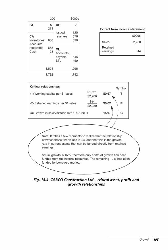
Growth 195
FA
CAInventoriesAccountsreceivableCash
OF
Issuedreserves
CLAccountspayableSTL
320376
£
646450
1,792
271$
838
65528
1,792
2001
1,521
696
1,096
2,280
Critical relationships
$1,521$2,280
$0.67(1) Working capital per $1 sales
$44$2,280
$0.02(2) Retained earnings per $1 sales
(3) Growth in sales/historic rate 1997–2001
$000s
$000s
Extract from income statement
T
R
Symbol
15% G
Note: It takes a few moments to realize that the relationshipbetween these two values is 3% and that this is the growthrate in current assets that can be funded directly from retainedearnings.
Actual growth is 15%, therefore only a fifth of growth has beenfunded from the internal resources. The remaining 12% has beenfunded by borrowed money.
Retainedearnings 44
Sales
Fig. 14.4 CABCO Construction Ltd – critical asset, profit andgrowth relationships
WKMR_CH14.QXD 11/24/05 12:40 PM Page 195
196 Key management ratios
Growth equilibrium
We use the term ‘growth equilibrium’ to identify the rate of growth that acompany can sustain from its operating cash flow. It means that cash is inequilibrium in the sense that it is driven neither into surplus nor deficitas a result of growth.
A growth equilibrium equation applicable to CABCO is given in figure14.5. The values for ‘R’, ‘T’ and ‘G’ have been identified in figure 14.4 andthese are combined together to produce the equilibrium factor ‘E’(Section A).
When E = 1, cash flow is neutral; values greater than 1 indicate a posi-tive cash flow and vice versa.*
The values for CABCO give a result of one over five, 20 percent(Section B). This is the fraction of the growth that is self-funded. It tellsus that 80 percent is funded from outside sources. The heavy borrowingthat the company has experienced derives from this fact.
The model has identified the three powerful cash flow drivers inthis company:
■ current assets to sales ■ retained earnings to sales■ growth in sales.
The company requires very high levels of inventory and accounts receiv-able to support sales. As sales expand rapidly these do likewise, therebycreating a great demand for cash. Retained profits are not adequate tomeet this need.
The model enables management to focus on the fundamental issuesfacing this company. These relate to profit, current assets and growth.Management must take steps to balance the relationship between thesethree so that the equilibrium value (‘E’) is increased from .02 up to 1.0.
Some scenarios are illustrated in figure 14.6.
%
* Many readers will have valid questions at this stage about the underlying assumptions inthe model. However, this is an early and primitive, but useful, version of a more generalizedgrowth model that will be developed later in the chapter.
WKMR_CH14.QXD 11/24/05 12:40 PM Page 196
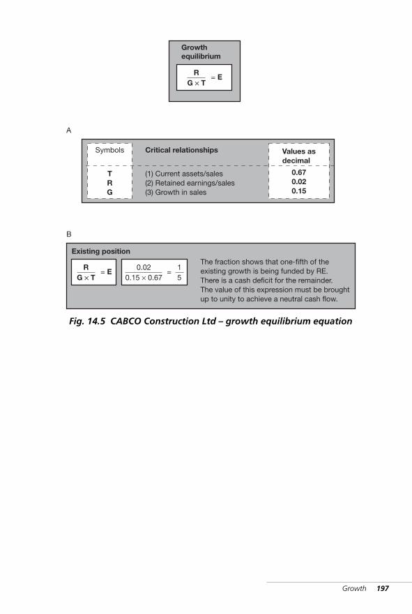
Growth 197
Critical relationships
(1) Current assets/sales(2) Retained earnings/sales(3) Growth in sales
Values asdecimal
0.670.020.15
RG × T
= E
RG × T
= E0.02
0.15 × 0.67=
15
The fraction shows that one-fifth of theexisting growth is being funded by RE.There is a cash deficit for the remainder.The value of this expression must be broughtup to unity to achieve a neutral cash flow.
Growthequilibrium
B
A
Existing position
TRG
Symbols
Fig. 14.5 CABCO Construction Ltd – growth equilibrium equation
WKMR_CH14.QXD 11/24/05 12:40 PM Page 197
198 Key management ratios
Growth equilibrium – scenarios
As stated above, management can focus on the essential elements of theproblem. The three variables must be brought into balance so that theresulting equilibrium value ‘E’ is increased to at least 1.0. This is the posi-tion where the company does not have to seek any further outside funds.
In figure 14.6 three single-value scenarios are worked out, one each for:
1. Growth
2. Retained profit
3. The current assets/sales ratio.
Each one shows the change in that variable alone that would be requiredto achieve equilibrium. It is not likely that any one of these in isolationwould be the most practical solution. A strategy involving elements of allthree would be more likely to bring results. The final combination strat-egy is shown as an illustration.
This version of the growth model is built up from the relationships thatexist between between current assets, retained earnings and growth in aparticular company.
It gives valid results for a company in the situation of CABCOConstruction Ltd. This company is heavily current-assets-based and veryheavily borrowed. The version is also useful, with slight amendments, fortrading companies and rapidly growing small businesses.
However for companies with a more regular asset structure and withnormal debt potential, a model with a more general application is needed.Such a model is introduced in the next section.
%
WKMR_CH14.QXD 11/24/05 12:40 PM Page 198
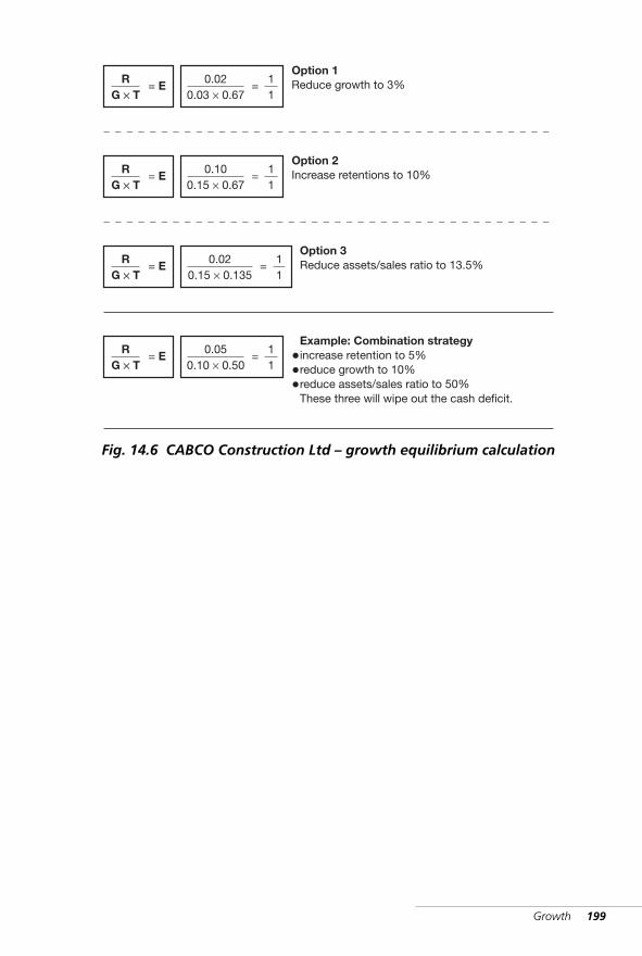
Growth 199
RG × T
= E0.02
0.03 × 0.67=
11
Option 1Reduce growth to 3%
RG × T
= E0.10
0.15 × 0.67=
11
Option 2Increase retentions to 10%
RG × T
= E0.02
0.15 × 0.135=
11
Option 3Reduce assets/sales ratio to 13.5%
RG × T
= E0.05
0.10 × 0.50=
11
•••
Example: Combination strategyincrease retention to 5%reduce growth to 10%reduce assets/sales ratio to 50%These three will wipe out the cash deficit.
Fig. 14.6 CABCO Construction Ltd – growth equilibrium calculation
WKMR_CH14.QXD 11/24/05 12:40 PM Page 199
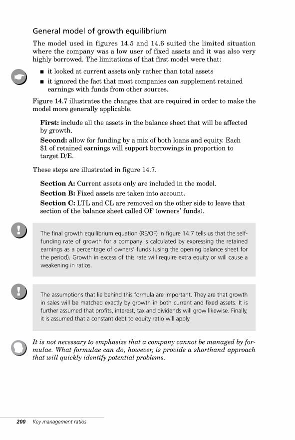
200 Key management ratios
General model of growth equilibrium
The model used in figures 14.5 and 14.6 suited the limited situationwhere the company was a low user of fixed assets and it was also veryhighly borrowed. The limitations of that first model were that:
■ it looked at current assets only rather than total assets ■ it ignored the fact that most companies can supplement retained
earnings with funds from other sources.
Figure 14.7 illustrates the changes that are required in order to make themodel more generally applicable.
First: include all the assets in the balance sheet that will be affectedby growth. Second: allow for funding by a mix of both loans and equity. Each $1 of retained earnings will support borrowings in proportion to target D/E.
These steps are illustrated in figure 14.7.
Section A: Current assets only are included in the model.Section B: Fixed assets are taken into account.Section C: LTL and CL are removed on the other side to leave thatsection of the balance sheet called OF (owners’ funds).
It is not necessary to emphasize that a company cannot be managed by for-mulae. What formulae can do, however, is provide a shorthand approachthat will quickly identify potential problems.
The final growth equilibrium equation (RE/OF) in figure 14.7 tells us that the self-funding rate of growth for a company is calculated by expressing the retainedearnings as a percentage of owners’ funds (using the opening balance sheet forthe period). Growth in excess of this rate will require extra equity or will cause aweakening in ratios.
!
The assumptions that lie behind this formula are important. They are that growthin sales will be matched exactly by growth in both current and fixed assets. It isfurther assumed that profits, interest, tax and dividends will grow likewise. Finally,it is assumed that a constant debt to equity ratio will apply.
!
☛
WKMR_CH14.QXD 11/24/05 12:40 PM Page 200
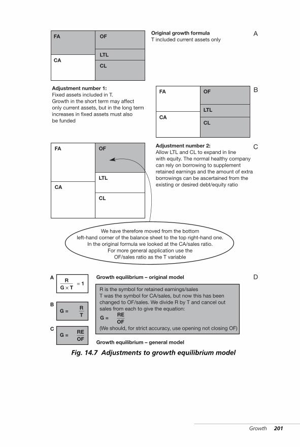
Growth 201
FA
CA
OF
LTL
CL
Original growth formulaT included current assets only
A
FA
CA
OF
LTL
CL
Adjustment number 1:Fixed assets included in T.Growth in the short term may affectonly current assets, but in the long termincreases in fixed assets must alsobe funded
B
FA
CA
OF
LTL
CL
Adjustment number 2:Allow LTL and CL to expand in linewith equity. The normal healthy companycan rely on borrowing to supplementretained earnings and the amount of extraborrowings can be ascertained from theexisting or desired debt/equity ratio
C
We have therefore moved from the bottomleft-hand corner of the balance sheet to the top right-hand one.
In the original formula we looked at the CA/sales ratio.For more general application use the
OF/sales ratio as the T variable
RG × T
= 1D
RT
G =
REOF
G =
A
B
C
Growth equilibrium – original model
R is the symbol for retained earnings/salesT was the symbol for CA/sales, but now this has beenchanged to OF/sales. We divide R by T and cancel outsales from each to give the equation:
(We should, for strict accuracy, use opening not closing OF)
Growth equilibrium – general model
REOF
G =
Fig. 14.7 Adjustments to growth equilibrium model
WKMR_CH14.QXD 11/24/05 12:40 PM Page 201
202 Key management ratios
Self-funding growth – international standards
Figure 14.8 shows two charts relating to the international scene.Chart A is derived from research done with top UK companies in 2000,
and chart B relates to research on international companies.Both indicate that large international companies have sustainable
growth rates of between 10 and 20 percent, except Japan with approxi-mately 7 percent. These are all very high numbers. With inflation as lowas 3 to 4 percent it suggests that they have the capacity to expand in realterms at well over 8 percent. If their actual growth is less then they willsimply accumulate cash in the balance sheet.
Given that the developed economies, in stable times over the long term,grow at 4 percent maximum, these companies are significantly outgrow-ing the economy. One can see why so many of them are involved intakeover activity. We have seen that these companies are also very prof-itable and many of them find it difficult to acquire companies that will notdilute their profit performance.
Some have found another outlet for surplus cash which is to buy backtheir own shares in the marketplace. This is a phenomenon that can nowbe observed with many large profitable companies.
Application to acquisitions
Many groups acquire fast-growing businesses in order to sustain orenhance the growth rate of the parent. The cash flow characteristics ofsuch acquisitions are of crucial importance.
A company that has heavy asset requirements, and that grows rapidly,will need substantial funds to keep its balance sheet in good condition. Ifthe company is very profitable, these funds may be generated internally.However, if it has only medium or low profits, then funds will have to beprovided by the parent company. The total cost of such a company over anumber of years could be many times its original purchase price.
The most valuable business to own or buy is one with high growth andhigh profits. The least valuable one is not a low growth, low profit com-pany. Such a company is not worth very much, but it is not dangerous.The worst company is one with high growth and low profits. If such acompany also has a high asset to sales ratio, then it has, within itself, allthe makings of a financial disaster.
☛
%
WKMR_CH14.QXD 11/24/05 12:40 PM Page 202
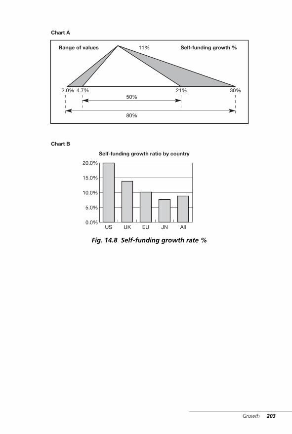
Growth 203
2.0% 4.7% 21% 30%50%
80%
11%Range of values
20.0%
15.0%
10.0%
5.0%
0.0%US
Self-funding growth ratio by country
UK EU JN All
Self-funding growth %
Chart A
Chart B
Fig. 14.8 Self-funding growth rate %
WKMR_CH14.QXD 11/24/05 12:40 PM Page 203

WKMR_CH14.QXD 11/24/05 12:40 PM Page 204
Part V Managementdecision-making
WKMR_CH15.QXD 11/24/05 12:45 PM Page 205

WKMR_CH15.QXD 11/24/05 12:45 PM Page 206
15 Cost, volumeand pricerelationshipsIntroduction · Costing illustration
· Contribution · Break-even (B/E)
· Contribution to sales percentage
(CPS) · Summary
Annual income twenty pounds, annualexpenditure nineteen pounds, nineteen shillingsand six pence result happiness. Annual incometwenty pounds, annual expenditure twentypounds, and six pence, result misery.CHARLES DICKENS (1812–1870) (Mr Micawber)
WKMR_CH15.QXD 11/24/05 12:45 PM Page 207

WKMR_CH15.QXD 11/24/05 12:45 PM Page 208
Cost, volume and price relationships 209
Introduction
The material covered to date has concerned itself with the company as asingle overall unit. In this chapter we probe down into the detailed opera-tions. Of course we find at this level that there are a multitude of separateproducts within the overall company. Each of these is a small business initself, and each has its own associated revenue and cost.
The internal operating dynamics of these sub-units can be quitecomplicated. We use a cost/management accounting system to give infor-mation and help to make decisions at this level. We would like to be in aposition where we can establish a total cost for a product, add on a profitmargin and then sell at the target selling price. Rarely are we able to dothis. The price we would like to charge is generally 10 percent above thatof our competitors. The manager is constantly being asked to get costsdown or to sell at or below the total cost figure.
It was mentioned earlier that the performance model which copes wellwith the big business scene is not good at this level of detail. However, itis at this level that profits are made and lost. Also, it is at this level thatday-to-day decisions are made as to what price to quote for a job, whetherto accept or reject a price on offer, whether and how to pay commission tosalespeople and so on.
The monthly management accounts supplied to managers are used bythem for decision-making. However, the way in which the information ispresented is often not helpful for this purpose. For instance, costs may beclassified in a way that does not allow their recalculation on the basis ofan alternative course of action.
This chapter will illustrate a series of calculations around this subjectthat enable managers to tread their way safely through these difficulties.These are essential, interesting and powerful tools. In the following pageswe will work through a number of examples that show their application.
How is it possible to make profits in this scenario? There is no magic answer, butwhat we can do is to recognize that the main function of cost accounting is notto arrive at a selling price but to identify the areas where profit is possible. Thismeans understanding how costs behave – in particular, how they respond tochanges in the variables: price, volume and, above all, product mix.
?
☛
WKMR_CH15.QXD 11/24/05 12:45 PM Page 209
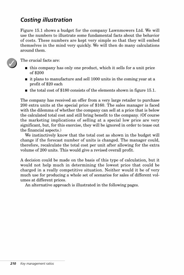
Costing illustration
Figure 15.1 shows a budget for the company Lawnmowers Ltd. We willuse the numbers to illustrate some fundamental facts about the behaviorof costs. These numbers are kept very simple so that they will embedthemselves in the mind very quickly. We will then do many calculationsaround them.
The crucial facts are:
■ this company has only one product, which it sells for a unit priceof $200
■ it plans to manufacture and sell 1000 units in the coming year at aprofit of $20 each
■ the total cost of $180 consists of the elements shown in figure 15.1.
The company has received an offer from a very large retailer to purchase200 extra units at the special price of $160. The sales manager is facedwith the dilemma of whether the company can sell at a price that is belowthe calculated total cost and still bring benefit to the company. (Of coursethe marketing implications of selling at a special low price are verysignificant, but, for this exercise, they will be ignored in order to tease outthe financial aspects.)
We instinctively know that the total cost as shown in the budget willchange if the forecast number of units is changed. The manager could,therefore, recalculate the total cost per unit after allowing for the extravolume of 200 units. This would give a revised overall profit.
A decision could be made on the basis of this type of calculation, but itwould not help much in determining the lowest price that could becharged in a really competitive situation. Neither would it be of verymuch use for producing a whole set of scenarios for sales of different vol-umes at different prices.
An alternative approach is illustrated in the following pages.
210 Key management ratios
✓
WKMR_CH15.QXD 11/24/05 12:45 PM Page 210
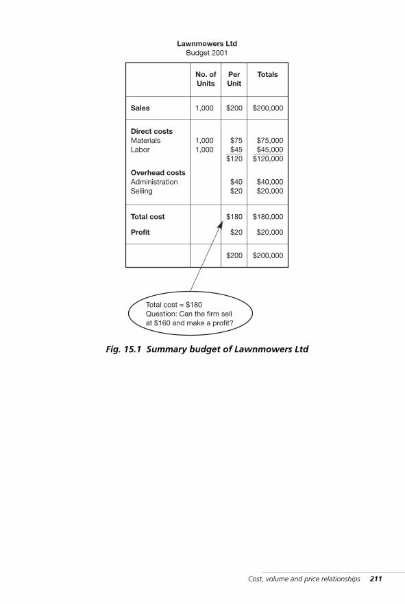
Cost, volume and price relationships 211
Sales
Direct costsMaterialsLabor
Overhead costsAdministrationSelling
Total cost
Profit
1,000
1,0001,000
No. ofUnits
$200
$75$45
$120
PerUnit
$40$20
$180
$20
$200
$200,000
$75,000$45,000
$120,000
Totals
$40,000$20,000
$180,000
$20,000
$200,000
Total cost = $180Question: Can the firm sellat $160 and make a profit?
Lawnmowers LtdBudget 2001
Fig. 15.1 Summary budget of Lawnmowers Ltd
WKMR_CH15.QXD 11/24/05 12:45 PM Page 211
212 Key management ratios
Cost classification
Of the many ways in which costs can be classified, possibly the mostuseful for decision-making purposes is on the basis of their response tovolume changes. This well-known classification uses the following terms:
■ Fixed costs: These are costs where the total expenditure does notchange with the level of activity. For instance rent of a factory willnot increase or decrease if volume of throughput goes up or down by10 percent.
■ Variable costs: These vary directly with changes in output. Thecost of materials consumed in the product will vary almost in directproportion to changes in volume.
An interesting paradox is that a fully variable cost is always a fixed chargeper unit irrespective of volume. On the other hand, fixed costs charged toeach unit fall with volume increases.
In practice, there are very few, if any, costs that are either totally fixedor totally variable across the whole range of possible outputs. However, itis useful for our example to make some simplifying assumptions. Thefixed and variable costs for Lawnmowers Ltd are shown in figure 15.2.
The variable costs are:
■ materials■ labor.
(In practice, while direct materials are almost always fully variable, directlabor is more than likely to be largely fixed.)
The fixed costs are assumed to be:
■ administration ■ selling.
(This assumption implies that these amounts will not change at all withany changes in volume.)
The variable and fixed costs per unit are $120 and $60 respectively. Theysum to a total cost of $180. Note that management is faced with the ques-tion of whether or not to accept a large order at a price of $160 per unit.
%
☛
WKMR_CH15.QXD 11/24/05 12:45 PM Page 212
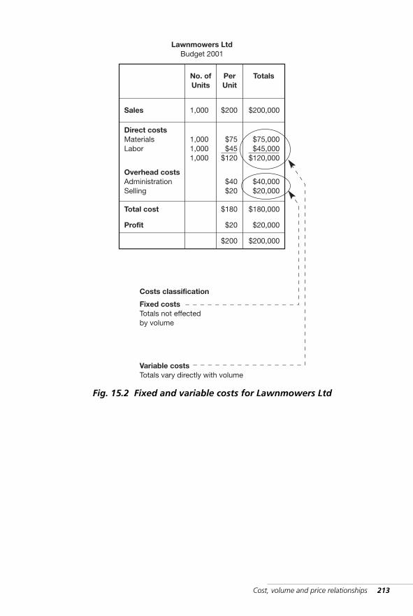
Cost, volume and price relationships 213
Sales
Direct costsMaterialsLabor
Overhead costsAdministrationSelling
Total cost
Profit
1,000
1,0001,0001,000
No. ofUnits
$200
$75$45
$120
PerUnit
$40$20
$180
$20
$200
$200,000
$75,000$45,000
$120,000
Totals
$40,000$20,000
$180,000
$20,000
$200,000
Fixed costsTotals not effectedby volume
Lawnmowers LtdBudget 2001
Variable costsTotals vary directly with volume
Costs classification
Fig. 15.2 Fixed and variable costs for Lawnmowers Ltd
WKMR_CH15.QXD 11/24/05 12:45 PM Page 213
Contribution
The division of costs into fixed and variable allows us to re-examine unitcosts. Figure 15.3 shows two different approaches to cost reporting:
■ total cost (traditional) approach ■ contribution approach.
In the traditional breakdown the unit selling price of $200 is split into:
■ variable cost $120■ fixed cost $60■ profit $20.
With the contribution approach, however, the selling price is split intojust two components:
■ variable cost of $120■ contribution of $80.
Contribution, therefore, replaces the figures of fixed cost of $60 and profitof $20. We remove the fixed cost charge from the product. The concept ofcontribution is important and useful. It is worthwhile spending some timeexamining it.
Cash flow and contribution
We have arrived at the contribution figure of $80 by adding back the fixedcost of $60 to the profit of $20. However, we can see that the same figureis arrived at when we deduct variable cost from the selling price, i.e. $200– $120. This latter definition is the most useful one.
We will extract cash flow meaning from it. Each extra unit sold at thebudget price results in a cash in-flow of $200. However, this extra unitalso increases variable costs by $120. These are direct cash costs whichwill give rise to a corresponding cash out-flow. One extra unit sold givesrise to extra revenue of $200 and extra cash costs of $120. The differenceof $80, which we call contribution, is the net cash in-flow resulting froman extra unit sold.
The $80 cash sacrificed from the loss of one unit is even more obvious.If the company suffers the loss of one unit it loses $200 revenue but itsaves only $120. So the cash loss is $80.
Contribution can therefore be defined as the net cash flow from a singletransaction. In other words, it is the cash gained from the sale of an extraunit or the cash lost from the sale of one unit less.
The relationship of contribution to profit will be pursued in the fol-lowing pages.
214 Key management ratios
☛
%
WKMR_CH15.QXD 11/24/05 12:45 PM Page 214
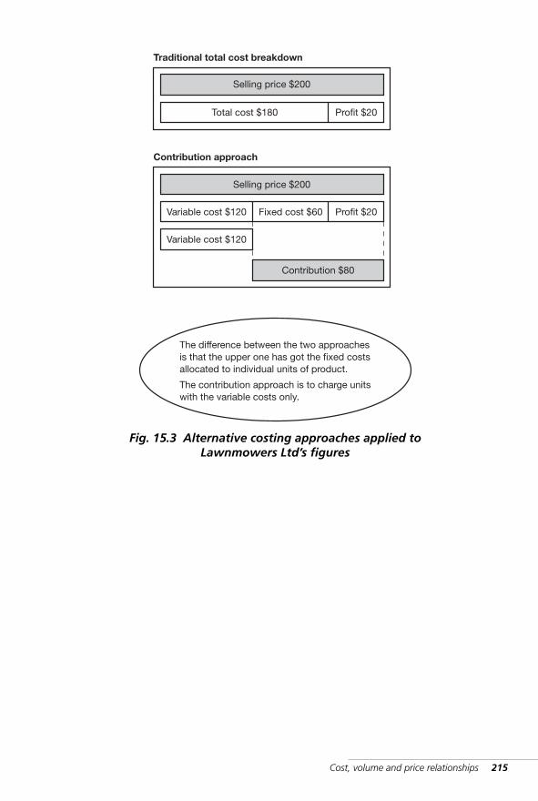
Cost, volume and price relationships 215
Traditional total cost breakdown
Total cost $180 Profit $20
Selling price $200
Contribution approach
Variable cost $120
Contribution $80
Profit $20
Selling price $200
Variable cost $120 Fixed cost $60
The difference between the two approachesis that the upper one has got the fixed costsallocated to individual units of product.
The contribution approach is to charge unitswith the variable costs only.
Fig. 15.3 Alternative costing approaches applied toLawnmowers Ltd’s figures
WKMR_CH15.QXD 11/24/05 12:45 PM Page 215
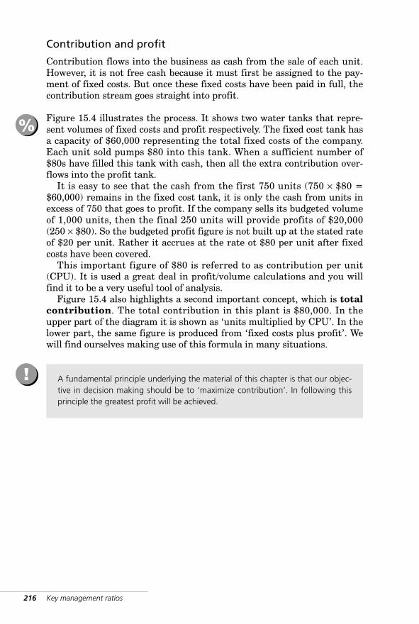
216 Key management ratios
Contribution and profit
Contribution flows into the business as cash from the sale of each unit.However, it is not free cash because it must first be assigned to the pay-ment of fixed costs. But once these fixed costs have been paid in full, thecontribution stream goes straight into profit.
Figure 15.4 illustrates the process. It shows two water tanks that repre-sent volumes of fixed costs and profit respectively. The fixed cost tank hasa capacity of $60,000 representing the total fixed costs of the company.Each unit sold pumps $80 into this tank. When a sufficient number of$80s have filled this tank with cash, then all the extra contribution over-flows into the profit tank.
It is easy to see that the cash from the first 750 units (750 × $80 =$60,000) remains in the fixed cost tank, it is only the cash from units inexcess of 750 that goes to profit. If the company sells its budgeted volumeof 1,000 units, then the final 250 units will provide profits of $20,000(250 × $80). So the budgeted profit figure is not built up at the stated rateof $20 per unit. Rather it accrues at the rate ot $80 per unit after fixedcosts have been covered.
This important figure of $80 is referred to as contribution per unit(CPU). It is used a great deal in profit/volume calculations and you willfind it to be a very useful tool of analysis.
Figure 15.4 also highlights a second important concept, which is totalcontribution. The total contribution in this plant is $80,000. In theupper part of the diagram it is shown as ‘units multiplied by CPU’. In thelower part, the same figure is produced from ‘fixed costs plus profit’. Wewill find ourselves making use of this formula in many situations.
A fundamental principle underlying the material of this chapter is that our objec-tive in decision making should be to ‘maximize contribution’. In following thisprinciple the greatest profit will be achieved.
!
%
WKMR_CH15.QXD 11/24/05 12:45 PM Page 216
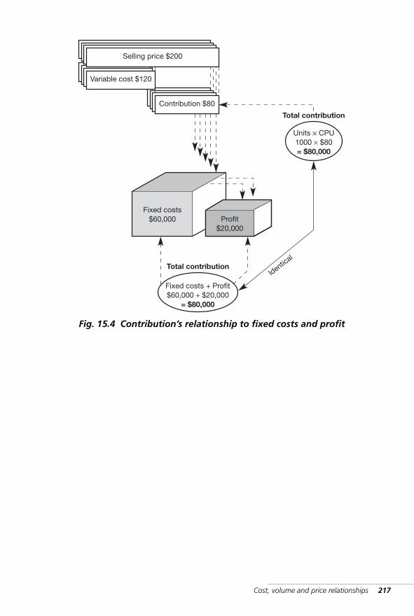
Cost, volume and price relationships 217
Contribution $80
Variable cost $120
Fixed costs$60,000
Selling price $200
Units × CPU1000 × $80= $80,000
Fixed costs + Profit$60,000 + $20,000
= $80,000
Identical
Total contribution
Total contribution
Profit$20,000
Fig. 15.4 Contribution’s relationship to fixed costs and profit
WKMR_CH15.QXD 11/24/05 12:45 PM Page 217
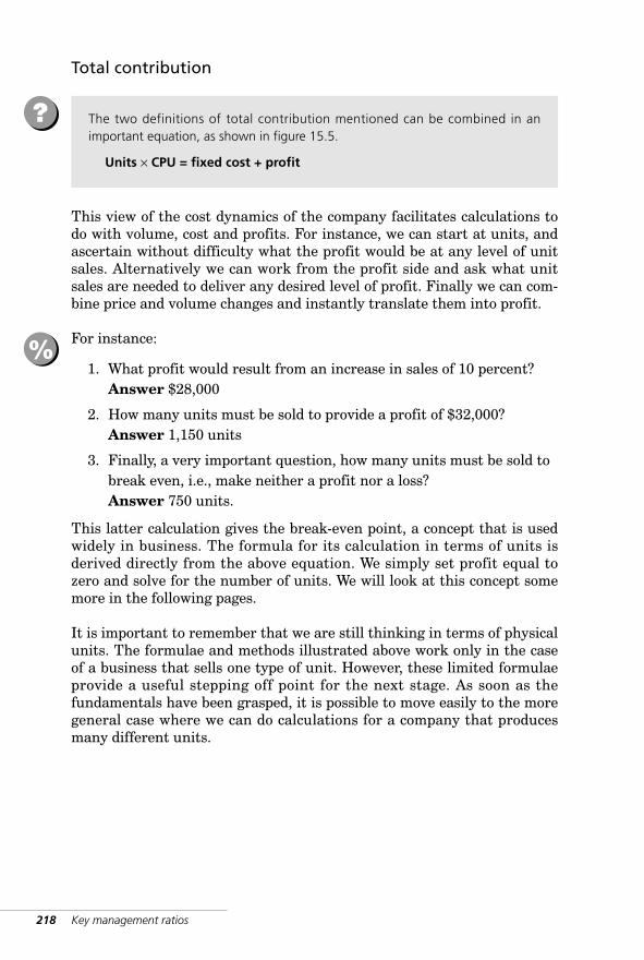
218 Key management ratios
Total contribution
This view of the cost dynamics of the company facilitates calculations todo with volume, cost and profits. For instance, we can start at units, andascertain without difficulty what the profit would be at any level of unitsales. Alternatively we can work from the profit side and ask what unitsales are needed to deliver any desired level of profit. Finally we can com-bine price and volume changes and instantly translate them into profit.
For instance:
1. What profit would result from an increase in sales of 10 percent?Answer $28,000
2. How many units must be sold to provide a profit of $32,000?Answer 1,150 units
3. Finally, a very important question, how many units must be sold tobreak even, i.e., make neither a profit nor a loss?Answer 750 units.
This latter calculation gives the break-even point, a concept that is usedwidely in business. The formula for its calculation in terms of units isderived directly from the above equation. We simply set profit equal tozero and solve for the number of units. We will look at this concept somemore in the following pages.
It is important to remember that we are still thinking in terms of physicalunits. The formulae and methods illustrated above work only in the caseof a business that sells one type of unit. However, these limited formulaeprovide a useful stepping off point for the next stage. As soon as thefundamentals have been grasped, it is possible to move easily to the moregeneral case where we can do calculations for a company that producesmany different units.
%
The two definitions of total contribution mentioned can be combined in animportant equation, as shown in figure 15.5.
Units × CPU = fixed cost + profit
?
WKMR_CH15.QXD 11/24/05 12:45 PM Page 218
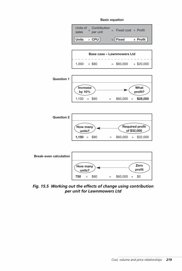
Cost, volume and price relationships 219
1,000 × $80 = $60,000 + $20,000
Question 1
Increaseby 10%
1,100 × $80 = $60,000 + $28,000
Whatprofit?
Question 2
How manyunits?
1,150 × $80 = $60,000 + $32,000
Required profitof $32,000
Break-even calculation
How manyunits?
750 × $80 = $60,000 + $0
Zeroprofit
Units ofsales
Contributionper unit× = Fixed cost + Profit
Units × CPU = Fixed + Profit
Basic equation
Base case – Lawnmowers Ltd
Fig. 15.5 Working out the effects of change using contribution per unit for Lawnmowers Ltd
WKMR_CH15.QXD 11/24/05 12:45 PM Page 219
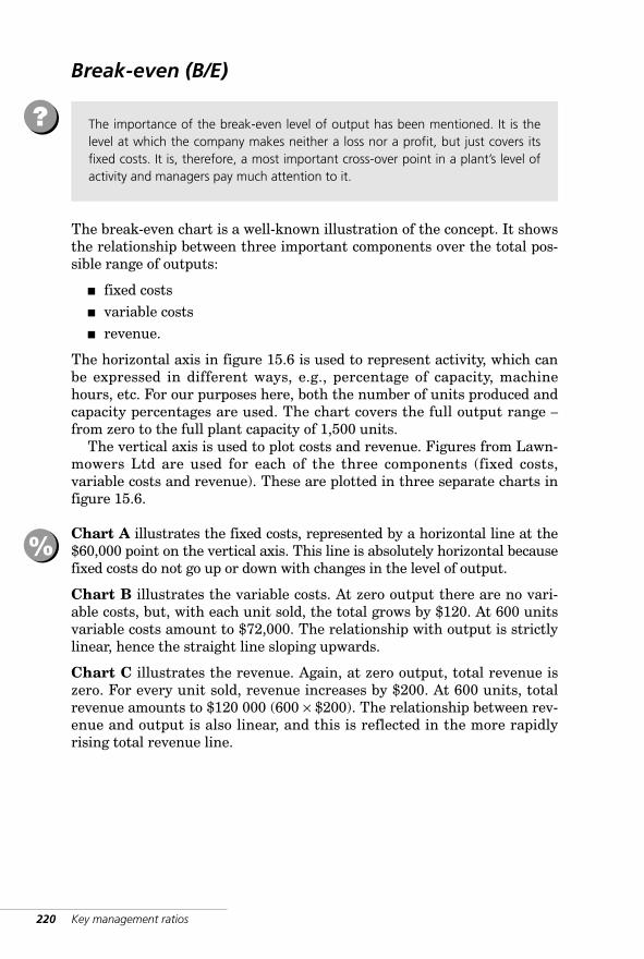
220 Key management ratios
Break-even (B/E)
The break-even chart is a well-known illustration of the concept. It showsthe relationship between three important components over the total pos-sible range of outputs:
■ fixed costs ■ variable costs ■ revenue.
The horizontal axis in figure 15.6 is used to represent activity, which canbe expressed in different ways, e.g., percentage of capacity, machinehours, etc. For our purposes here, both the number of units produced andcapacity percentages are used. The chart covers the full output range –from zero to the full plant capacity of 1,500 units.
The vertical axis is used to plot costs and revenue. Figures from Lawn-mowers Ltd are used for each of the three components (fixed costs,variable costs and revenue). These are plotted in three separate charts infigure 15.6.
Chart A illustrates the fixed costs, represented by a horizontal line at the$60,000 point on the vertical axis. This line is absolutely horizontal becausefixed costs do not go up or down with changes in the level of output.
Chart B illustrates the variable costs. At zero output there are no vari-able costs, but, with each unit sold, the total grows by $120. At 600 unitsvariable costs amount to $72,000. The relationship with output is strictlylinear, hence the straight line sloping upwards.
Chart C illustrates the revenue. Again, at zero output, total revenue iszero. For every unit sold, revenue increases by $200. At 600 units, totalrevenue amounts to $120 000 (600 × $200). The relationship between rev-enue and output is also linear, and this is reflected in the more rapidlyrising total revenue line.
%
The importance of the break-even level of output has been mentioned. It is thelevel at which the company makes neither a loss nor a profit, but just covers itsfixed costs. It is, therefore, a most important cross-over point in a plant’s level ofactivity and managers pay much attention to it.
?
WKMR_CH15.QXD 11/24/05 12:45 PM Page 220
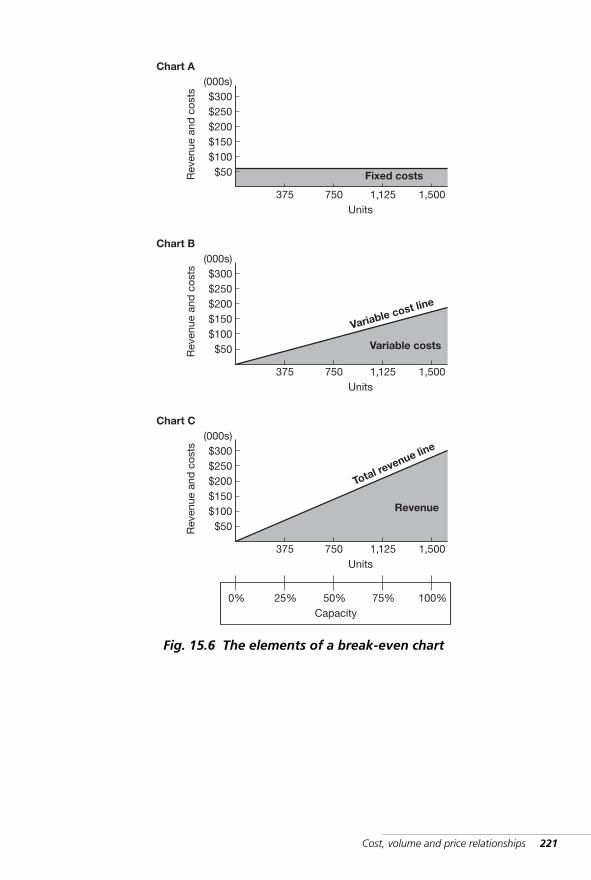
Cost, volume and price relationships 221
$50$100$150$200$250$300
(000s)
375 750 1,125 1,500Units
Rev
enue
and
cos
ts
Chart A
$50$100$150$200$250$300
(000s)
375 750 1,125 1,500Units
Rev
enue
and
cos
ts
Chart B
$50$100$150$200$250$300
(000s)
375 750 1,125 1,500Units
Rev
enue
and
cos
ts
Chart C
Fixed costs
Variable costs
Revenue
Variable cost line
Total revenue line
25% 50% 75% 100%Capacity
0%
Fig. 15.6 The elements of a break-even chart
WKMR_CH15.QXD 11/24/05 12:45 PM Page 221
222 Key management ratios
Break-even (B/E) Chart
In figure 15.7, the three separate charts of figure 15.6 have been com-bined to show how the three sections come together. First we see the bandof fixed costs at the base of the chart. Positioned above this is the variablecosts wedge. Along the upper boundary of this wedge is the total cost line.Finally, the total revenue line is shown rising from the zero revenue atzero output up through the two areas of cost until it breaks through thetotal cost line about 50 percent of capacity. This is the break-even point.To the left of it lies loss, to the right profit.
The break-even point here occurs at a level of 750 units which equatesto revenue of $150,000. Remember from figure 15.5 that 750 unitswill result in a contribution of $60,000 (750 × $80), which just equals thefixed cost.
A line is plotted representing the budgeted sales of 1,000 units at a unitprice of $200. This puts the company a little way to the right of the break-even point. The surplus output over break even is sometimes referred to asthe ‘margin of safety’. This margin of safety here is 25 percent, which meansthat sales can fall by this percentage before the break-even point is reached.
A number of simplifying assumptions are incorporated into this chart. Ithas been assumed that (1) fixed costs are totally fixed for all levels ofoutput, (2) that unit variable costs do not change irrespective of numbersproduced and (3) that unit revenue is the same for all levels of sales.These assumptions may be valid over a fairly narrow range on each sideof existing levels of activity. At very low or very high levels, however, theassumptions break down and the chart ceases to be accurate.
Notwithstanding these limitations, the break-even chart is a useful toolfor presenting information, for explaining the dynamics of a productionunit, for pointing out the essential features of the volume, cost and rev-enue system and for setting minimum sales targets.
☛
%
WKMR_CH15.QXD 11/24/05 12:45 PM Page 222
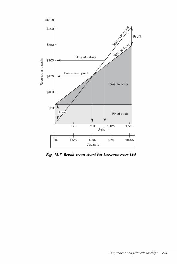
Cost, volume and price relationships 223
375
$50
$100
$150
$200
$250
$300
750 1,125 1,500
Variable costs
Fixed costs
Profit
Tota
l rev
enue
line
Total c
ost lin
e
Budget values
Break-even point
(000s)
Rev
enue
and
cos
ts
Units
25% 50% 75% 100%0%Capacity
Loss
Fig. 15.7 Break-even chart for Lawnmowers Ltd
WKMR_CH15.QXD 11/24/05 12:45 PM Page 223
224 Key management ratios
Figure 15.8 shows charts for two types of company. The first (A) has ahigh operating leverage. With high fixed costs and low unit variable costsit has a total cost line that starts high on the chart but has a relatively flattrajectory. The total revenue line cuts the total cost line at quite a wideangle, which means that profit increases rapidly to the right of the break-even point. Unfortunately, to the left of this point, the negative gap alsowidens rapidly, meaning that the company gets into heavy losses veryquickly as output falls away.
The second (B) has a low operating leverage. This company has low fixedcosts but high unit variable costs. The total cost line starts low but climbssteeply with increased volume. The total revenue line produces a muchnarrower angle at the crossover point, indicating that both profits andlosses grow more slowly either right or left of the break-even point.
In Company A, we can understand there is intense pressure to achievevolume sales in order to move out of the heavy loss situation to the left ofthe break-even point. And when the break-even point has been reached,there is the prize of a rapidly increasing profit figure to provide the incen-tive to achieve even greater volume. When total production capacityexceeds total demand, fierce price competition can erupt between firms ofthis type as they compete for volume. The companies with this cost profileare those with heavy fixed assets, such as steel and transport companies.
The second situation, with low operating leverage, is frequently foundto exist in companies with smaller, flexible production systems and lowfixed assets. These companies tend to have less risk, but also less reward,attached to them.
This chart can also be used to identify companies with different cost structuresand therefore different levels of what is called ‘operating leverage’. Operatingleverage identifies the change in profit that results from a small change in sales,e.g., if a 10 percent change in sales produces a 40 percent change in profit, thenwe say that the company has a high operating leverage of 4 times.
?
%
WKMR_CH15.QXD 11/24/05 12:45 PM Page 224
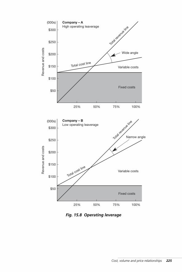
Cost, volume and price relationships 225
$50
$100
$150
$200
$250
$300
(000s)
25% 50% 75% 100%
Company – AHigh operating leaverage
$50
$100
$150
$200
$250
$300
(000s)
Fixed costs
Fixed costs
Total cost lineVariable costs
Tota
l reve
nue l
ine
Wide angle
Variable costs
Total cost line
Tota
l reve
nue l
ine
Narrow angle
25% 50% 75% 100%
Rev
enue
and
cos
tsR
even
ue a
nd c
osts
Company – BLow operating leaverage
Fig. 15.8 Operating leverage
WKMR_CH15.QXD 11/24/05 12:45 PM Page 225
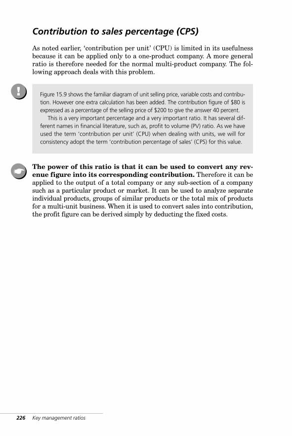
226 Key management ratios
Contribution to sales percentage (CPS)
As noted earlier, ‘contribution per unit’ (CPU) is limited in its usefulnessbecause it can be applied only to a one-product company. A more generalratio is therefore needed for the normal multi-product company. The fol-lowing approach deals with this problem.
The power of this ratio is that it can be used to convert any rev-enue figure into its corresponding contribution. Therefore it can beapplied to the output of a total company or any sub-section of a companysuch as a particular product or market. It can be used to analyze separateindividual products, groups of similar products or the total mix of productsfor a multi-unit business. When it is used to convert sales into contribution,the profit figure can be derived simply by deducting the fixed costs.
Figure 15.9 shows the familiar diagram of unit selling price, variable costs and contribu-tion. However one extra calculation has been added. The contribution figure of $80 isexpressed as a percentage of the selling price of $200 to give the answer 40 percent.
This is a very important percentage and a very important ratio. It has several dif-ferent names in financial literature, such as, profit to volume (PV) ratio. As we haveused the term ‘contribution per unit’ (CPU) when dealing with units, we will forconsistency adopt the term ‘contribution percentage of sales’ (CPS) for this value.
!
☛
WKMR_CH15.QXD 11/24/05 12:45 PM Page 226
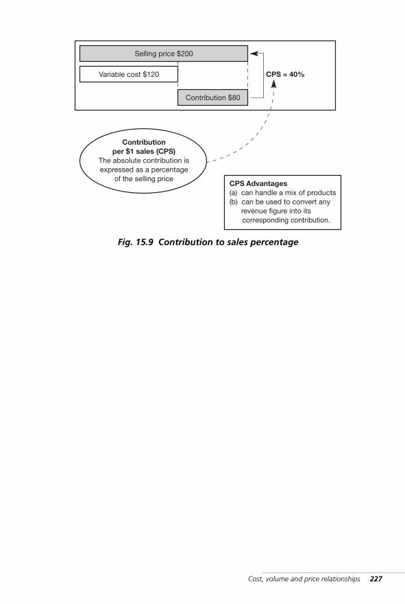
Cost, volume and price relationships 227
Variable cost $120
Contribution $80
Selling price $200
CPS Advantages(a) can handle a mix of products(b) can be used to convert any(a) revenue figure into its(a) corresponding contribution.
CPS = 40%
Contributionper $1 sales (CPS)
The absolute contribution isexpressed as a percentage
of the selling price
Fig. 15.9 Contribution to sales percentage
WKMR_CH15.QXD 11/24/05 12:45 PM Page 227
228 Key management ratios
Total contribution – alternate views
However it can also be derived from three separate sources (see figure 15.10):
■ units × CPU ■ revenue × CPS ■ fixed costs + profit.
We can take the latter two and derive the identity:
Revenue × CPS = Fixed costs + Profit
Given the four variables in this equation, if we know any three of themwe can find the remaining one.
Answer: ($35,000 × 22% – $3,800) = $3,900
Further examples are given in the next section.
Revenue ? × $35,000 ×
CPS × ? 22% ×
Fixed costs × × ? ×
Profit × × $3,800 ?
It is important at this point to distinguish between unit contribution and thetotal contribution of the whole plant.
Unit contribution is simply the selling price less the variable costs figure forone unit.
Similarly total contribution is total revenue less total variable costs.
!
%
WKMR_CH15.QXD 11/24/05 12:45 PM Page 228
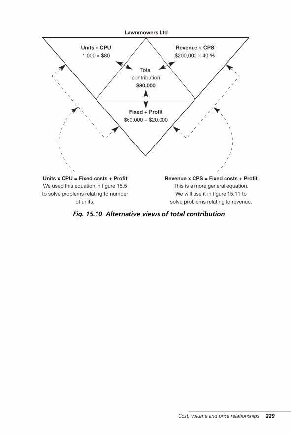
Cost, volume and price relationships 229
Total
contribution
$80,000
Fixed + Profit
$60,000 + $20,000
Units × CPU
1,000 × $80
Revenue × CPS
$200,000 × 40 %
Units x CPU = Fixed costs + Profit
We used this equation in figure 15.5
to solve problems relating to number
of units.
Lawnmowers Ltd
Revenue x CPS = Fixed costs + Profit
This is a more general equation.
We will use it in figure 15.11 to
solve problems relating to revenue.
Fig. 15.10 Alternative views of total contribution
WKMR_CH15.QXD 11/24/05 12:45 PM Page 229
230 Key management ratios
Problem solving using CPS
We use the identity between the expressions:
1. Revenue × CPS and
2. fixed costs plus profit
to solve problems in figure 15.11. The problems illustrated here are the same as in figure 15.5, except that
‘contribution to sales percentage’ (CPS) has been used in place of ‘contributionper unit’ (CPU). Results are expressed in money terms rather than in unitswhich is generally more useful. By converting units @ $200 sales price we seethat the answers achieved by both approaches are identical.
As an extra example, consider the following:
■ Budgeted sales for Lawnmowers Ltd are $200,000. ■ At a CPS of 40 percent the budgeted contribution is $80,000. ■ If the revenue figure were to fall to $180,000, the resulting
contribution would be $72,000 ($180,000 × 40 percent). ■ The profit from this reduced level of sales would be $12,000. ■ ($72,000 contribution – $60,000 fixed cost = $12,000 profit).
%
WKMR_CH15.QXD 11/24/05 12:45 PM Page 230
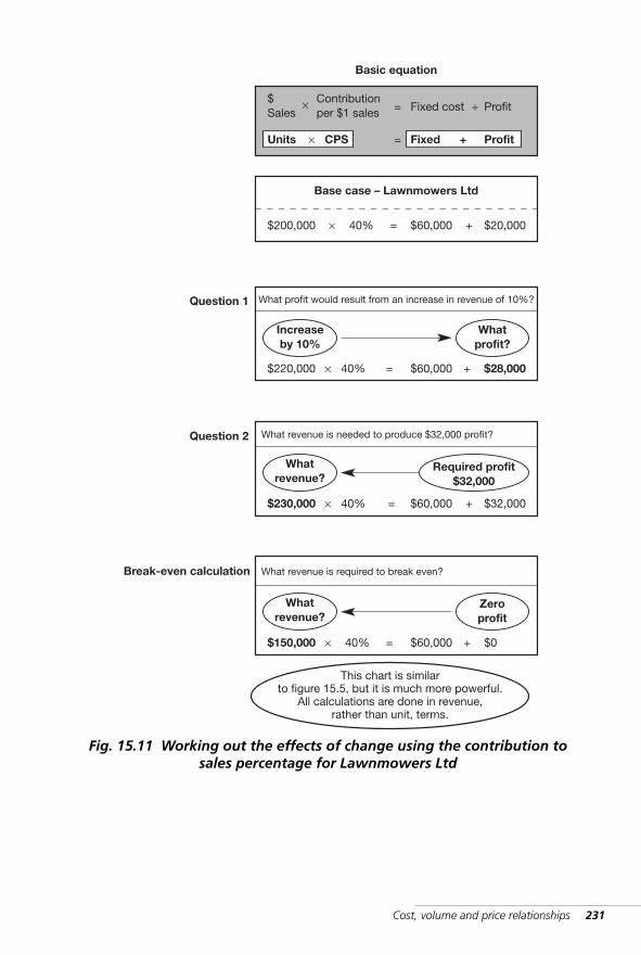
Cost, volume and price relationships 231
$200,000 × 40% = $60,000 + $20,000
What profit would result from an increase in revenue of 10%?
Increaseby 10%
$220,000 × 40% = $60,000 + $28,000
Whatprofit?
What revenue is needed to produce $32,000 profit?
Whatrevenue?
$230,000 × 40% = $60,000 + $32,000
Required profit$32,000
What revenue is required to break even?
Whatrevenue?
$150,000 × 40% = $60,000 + $0
Zeroprofit
$Sales
Contributionper $1 sales
× = Fixed cost + Profit
Units × CPS = Fixed + Profit
Basic equation
Base case – Lawnmowers Ltd
Question 1
Question 2
Break-even calculation
This chart is similarto figure 15.5, but it is much more powerful.
All calculations are done in revenue,rather than unit, terms.
Fig. 15.11 Working out the effects of change using the contribution tosales percentage for Lawnmowers Ltd
WKMR_CH15.QXD 11/24/05 12:45 PM Page 231
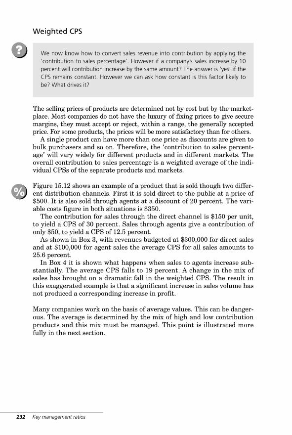
232 Key management ratios
Weighted CPS
The selling prices of products are determined not by cost but by the market-place. Most companies do not have the luxury of fixing prices to give securemargins, they must accept or reject, within a range, the generally acceptedprice. For some products, the prices will be more satisfactory than for others.
A single product can have more than one price as discounts are given tobulk purchasers and so on. Therefore, the ‘contribution to sales percent-age’ will vary widely for different products and in different markets. Theoverall contribution to sales percentage is a weighted average of the indi-vidual CPSs of the separate products and markets.
Figure 15.12 shows an example of a product that is sold though two differ-ent distribution channels. First it is sold direct to the public at a price of$500. It is also sold through agents at a discount of 20 percent. The vari-able costs figure in both situations is $350.
The contribution for sales through the direct channel is $150 per unit,to yield a CPS of 30 percent. Sales through agents give a contribution ofonly $50, to yield a CPS of 12.5 percent.
As shown in Box 3, with revenues budgeted at $300,000 for direct salesand at $100,000 for agent sales the average CPS for all sales amounts to25.6 percent.
In Box 4 it is shown what happens when sales to agents increase sub-stantially. The average CPS falls to 19 percent. A change in the mix ofsales has brought on a dramatic fall in the weighted CPS. The result inthis exaggerated example is that a significant increase in sales volume hasnot produced a corresponding increase in profit.
Many companies work on the basis of average values. This can be danger-ous. The average is determined by the mix of high and low contributionproducts and this mix must be managed. This point is illustrated morefully in the next section.
%
We now know how to convert sales revenue into contribution by applying the‘contribution to sales percentage’. However if a company’s sales increase by 10percent will contribution increase by the same amount? The answer is ‘yes’ if theCPS remains constant. However we can ask how constant is this factor likely tobe? What drives it?
?
WKMR_CH15.QXD 11/24/05 12:45 PM Page 232
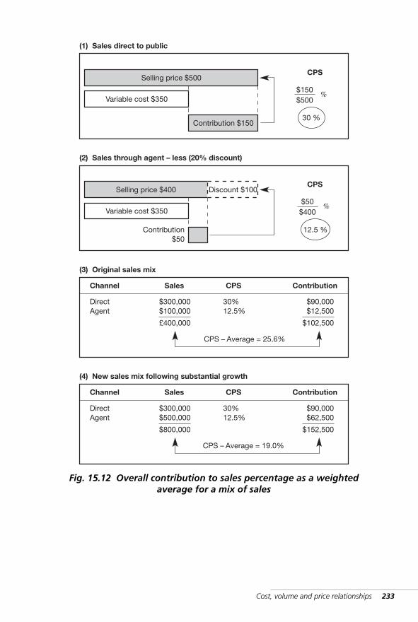
Cost, volume and price relationships 233
Selling price $400
Variable cost $350
Contribution $150
Selling price $500CPS
$150$500
%
30 %
Variable cost $350
Contribution$50
CPS
$50$400
%
12.5 %
Discount $100
Channel
DirectAgent
Sales
$300,000$100,000
CPS
30%12.5%
Contribution
$90,000$12,500
£400,000 $102,500
CPS – Average = 25.6%
Channel
DirectAgent
Sales
$300,000$500,000
CPS
30%12.5%
Contribution
$90,000$62,500
$800,000 $152,500
CPS – Average = 19.0%
(1) Sales direct to public
(2) Sales through agent – less (20% discount)
(3) Original sales mix
(4) New sales mix following substantial growth
Fig. 15.12 Overall contribution to sales percentage as a weightedaverage for a mix of sales
WKMR_CH15.QXD 11/24/05 12:45 PM Page 233
234 Key management ratios
Product mix
In figure 15.13, data is given about a company that sells three products (A,B and C) through two distribution networks (direct and through agents).There are, therefore, six product-market segments as shown in the matrixin the top right-hand corner. The contribution to sales percentage for eachsegment is shown in the matrix in the upper right-hand corner.
Budgeted and actual sales of the product market segments are shown.Beneath these, the contributions from the two sets of data have beencalculated.
As shown by the arrows, the sales value in each segment is multiplied byits corresponding CPS to arrive at its contribution. The contributions fromthe individual segments are accumulated to give the total contribution.
Fixed costs are $75,000 for both budgeted and actual results, and theseare deducted to give the final budgeted and actual profit. A budgetedprofit of $16,000 has turned into an actual loss of $1,000.
In comparing budgeted with actual figures, note the following:
■ total revenue of $300,000 is unchanged ■ selling prices are unchanged■ cost per unit figures are unchanged ■ fixed costs are unchanged■ budgeted profit is converted into an actual loss.
The sole reason for this adverse turnaround is to be found in the mixof products.
The bulk of sales has moved from high to low contribution segments.For example, in the bottom right-hand last segment, which has the lowestCPS value (product C sold through agents), sales have increased from abudgeted $20,000 to an actual $60,000. This increase has been offset byreductions in the better segments. Similar other adverse movements canbe identified. The overall product mix has been diluted and the companyhas suffered grievously.
Product mix is a potent driver of profit. It must be identified, understood by alland positively managed to achieve maximum potential.
!
%
WKMR_CH15.QXD 11/24/05 12:45 PM Page 234
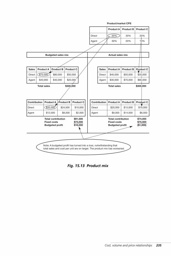
Cost, volume and price relationships 235
Product A Product B Product C
Direct
Agent
Product/market CPS
50%
30%
30%
20%
20%
Sales Product A Product C
Direct
Agent
$70,000
$40,000
$80,000
$40,000
$50,000
Total sales
Contribution Product A Product C
Direct
Agent
$35,000
$12,000
$24,000
$8,000
$10,000
$2,000
$91,000$75,000$16,000
Total contributionFixed costsBudgeted profit
Sales Product A Product B
Direct
Agent
$40,000
$30,000
$50,000
$70,000
Total sales
Contribution Product A Product B
Direct
Agent
$20,000
$9,000
$15,000
$14,000
$10,000
$6,000
$74,000$75,000($1,000)
Total contributionFixed costsBudgeted profit
Actual sales mixBudgeted sales mix
Note: A budgeted profit has turned into a loss, notwithstanding thattotal sales and cost per unit are on target. The product mix has worsened.
10%
Product C
$50,000
$60,000
$300,000
Product C
Product B
$20,000
$300,000
Product B
Fig. 15.13 Product mix
WKMR_CH15.QXD 11/24/05 12:45 PM Page 235
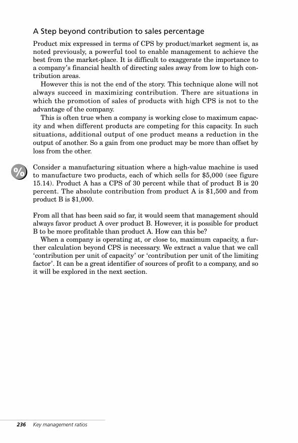
236 Key management ratios
A Step beyond contribution to sales percentage
Product mix expressed in terms of CPS by product/market segment is, asnoted previously, a powerful tool to enable management to achieve thebest from the market-place. It is difficult to exaggerate the importance toa company’s financial health of directing sales away from low to high con-tribution areas.
However this is not the end of the story. This technique alone will notalways succeed in maximizing contribution. There are situations inwhich the promotion of sales of products with high CPS is not to theadvantage of the company.
This is often true when a company is working close to maximum capac-ity and when different products are competing for this capacity. In suchsituations, additional output of one product means a reduction in theoutput of another. So a gain from one product may be more than offset byloss from the other.
Consider a manufacturing situation where a high-value machine is usedto manufacture two products, each of which sells for $5,000 (see figure15.14). Product A has a CPS of 30 percent while that of product B is 20percent. The absolute contribution from product A is $1,500 and fromproduct B is $1,000.
From all that has been said so far, it would seem that management shouldalways favor product A over product B. However, it is possible for productB to be more profitable than product A. How can this be?
When a company is operating at, or close to, maximum capacity, a fur-ther calculation beyond CPS is necessary. We extract a value that we call‘contribution per unit of capacity’ or ‘contribution per unit of the limitingfactor’. It can be a great identifier of sources of profit to a company, and soit will be explored in the next section.
%
WKMR_CH15.QXD 11/24/05 12:45 PM Page 236
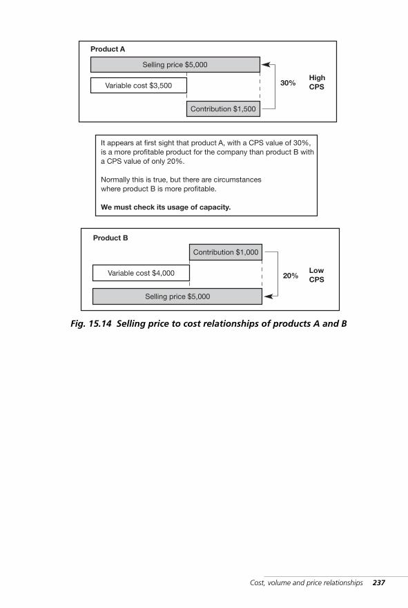
Cost, volume and price relationships 237
Variable cost $3,500
Contribution $1,500
Selling price $5,000
30%
Product A
Variable cost $4,000
Contribution $1,000
Selling price $5,000
Product B
It appears at first sight that product A, with a CPS value of 30%,is a more profitable product for the company than product B witha CPS value of only 20%.
Normally this is true, but there are circumstanceswhere product B is more profitable.
We must check its usage of capacity.
HighCPS
20%LowCPS
Fig. 15.14 Selling price to cost relationships of products A and B
WKMR_CH15.QXD 11/24/05 12:45 PM Page 237
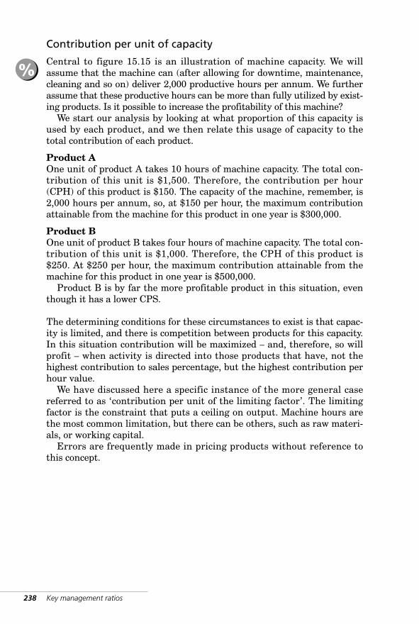
238 Key management ratios
Contribution per unit of capacity
Central to figure 15.15 is an illustration of machine capacity. We willassume that the machine can (after allowing for downtime, maintenance,cleaning and so on) deliver 2,000 productive hours per annum. We furtherassume that these productive hours can be more than fully utilized by exist-ing products. Is it possible to increase the profitability of this machine?
We start our analysis by looking at what proportion of this capacity isused by each product, and we then relate this usage of capacity to thetotal contribution of each product.
Product AOne unit of product A takes 10 hours of machine capacity. The total con-tribution of this unit is $1,500. Therefore, the contribution per hour(CPH) of this product is $150. The capacity of the machine, remember, is2,000 hours per annum, so, at $150 per hour, the maximum contributionattainable from the machine for this product in one year is $300,000.
Product BOne unit of product B takes four hours of machine capacity. The total con-tribution of this unit is $1,000. Therefore, the CPH of this product is$250. At $250 per hour, the maximum contribution attainable from themachine for this product in one year is $500,000.
Product B is by far the more profitable product in this situation, eventhough it has a lower CPS.
The determining conditions for these circumstances to exist is that capac-ity is limited, and there is competition between products for this capacity.In this situation contribution will be maximized – and, therefore, so willprofit – when activity is directed into those products that have, not thehighest contribution to sales percentage, but the highest contribution perhour value.
We have discussed here a specific instance of the more general casereferred to as ‘contribution per unit of the limiting factor’. The limitingfactor is the constraint that puts a ceiling on output. Machine hours arethe most common limitation, but there can be others, such as raw materi-als, or working capital.
Errors are frequently made in pricing products without reference tothis concept.
%
WKMR_CH15.QXD 11/24/05 12:45 PM Page 238
Cost, volume and price relationships 239
Variable cost $3,500
Contribution $1,500
Selling price $5,000
30%
Product A
Variable cost $4,000
Contribution $1,000
Selling price $5,000
20%
Machine hours available= 2,000 per annum
Hours used = 10
Hours used = 4
The low CPS product has a better rateof contribution per capacity hour.
Product B
HighCPS
Contributionper hour (CPH)
$1,500/10$150
LowCPS
Contributionper hour (CPH)
$1,000/4$250
Fig. 15.15 Contribution per machine hour of products A and B
WKMR_CH15.QXD 11/24/05 12:45 PM Page 239
Summary
It is important to:
■ Classify costs to distinguish fixed from variable■ Identify contribution by product group■ Actively direct sales from low to high contribution areas■ Where capacity hours are a constraint, identify and direct sales into
products with high CPH values.
240 Key management ratios
✓
WKMR_CH15.QXD 11/24/05 12:45 PM Page 240
16 InvestmentratiosIntroduction · Project appraisal –
the problem · Project appraisal –
steps to a solution (1) · Project
appraisal – steps to a solution (2)
· Project appraisal – present value
(PV) · Project appraisal – internal
rate of return (IRR) · Project
appraisal – summary
The social object of skilled investment shouldbe to defeat the dark forces of time andignorance which envelope our future.JOHN MAYNARD KEYNES (1883–1946)
WKMR_CH16.QXD 11/24/05 12:46 PM Page 241

WKMR_CH16.QXD 11/24/05 12:46 PM Page 242
Investment ratios 243
Introduction
The need for a company to earn a return on its investment has been cov-ered in detail. It is clear that this return must meet market expectationsif the standing and value of the company is not to suffer.
One of management’s critical functions is planning the future of thebusiness to ensure that an adequate rate of return is maintained. Essentialto this is adequate new productive investment, as it is the return on thisnew investment that will provide the ongoing profits on which the companydepends. Therefore a careful selection process needs to be applied to com-peting investment proposals so that only the best qualify.
In the past, many approaches have been adopted to assist managers inthis selection. One very well tried and tested one that is still in use, is‘pay-back’. Simply calculate the number of years that the project will taketo pay back the money invested in it. As a rule of thumb it can provide auseful ‘fix’ on a project. However, it is not a mathematically soundapproach. Some accounting-type measures have also been used in the pastthat are mathematically suspect.
This chapter is about the sound and tested techniques used now by allmajor companies to assist them with investment decisions. It illustratesthe various measures and ratios that have proved to be effective in select-ing and ranking investment projects.
☛
WKMR_CH16.QXD 11/24/05 12:46 PM Page 243
244 Key management ratios
Project appraisal – the problem
The standard investment profile is that of a large initial cash out-flow fol-lowed by a stream of cash in-flows for a certain number of years (sectionA of figure 16.1). The investor hopes that the in-flows will both repay theinitial investment and yield an adequate surplus. The problem has beenhow to relate the immediate cash outlay with the stream of future repay-ments so as to determine the true rate of return.
In section B of figure 16.1, the financial numbers are given forInvestment ‘X’. The investment is $1,000 and the stream of repaymentsover five years add up to $2,000. What, then, is the rate of return on theinvestment (ROI)? The increase in value over the five years is 100 per-cent, which could be interpreted as 20 percent per annum. Is this acorrect interpretation? Is the return adequate and how is it affected byinflation? These are the questions investors commonly ask. Beforeanswering them, let us look at one more example.
Section C of figure 16.1 shows the cash flows of Investment ‘Y’. Theinvestment here of $1,000 and total repayments of $2,000 is the same asbefore. However, the pattern of repayments is quite different. For each ofthe first four years the cash in-flows are $200 but in Year 5 the initialinvestment of $1,000 is repaid in addition to the annual amount of $200.In other words an investment of $1,000 gives an annual return of $200and, at the end of its life, the original investment of $1,000 is also repaidin full. This is the pattern of cash flows we would realize if we were toinvest in a fixed interest security yielding 20 percent. The true return onthis project is 20 percent.
When we look back at Investment X, we see that we do not get ourinvestment back in one lump at the end of the period – it is spread overeach year. The yearly cash repayments, then, are both paying interest onthe investments and repaying the principal. This is the pattern of returnsgiven by a commercial investment such as a piece of equipment thatwears out to nothing over a five year period. The return to the investorhere cannot be assessed so easily.
%
WKMR_CH16.QXD 11/24/05 12:46 PM Page 244
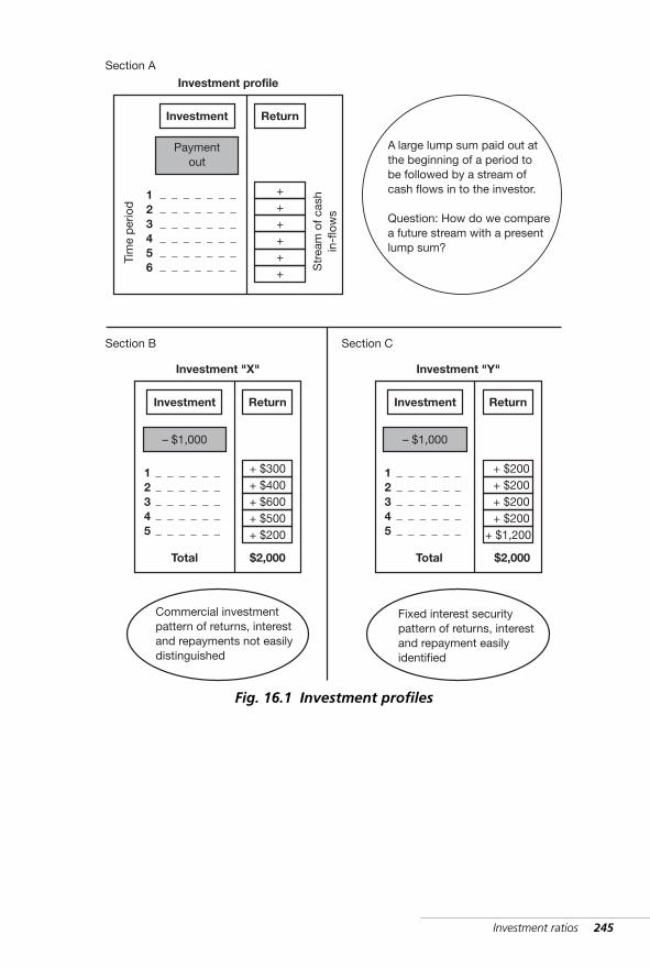
Investment ratios 245
Investment Return
Paymentout
123456
++++++ S
trea
m o
f cas
hin
-flo
ws
Tim
e p
erio
d
Section A
A large lump sum paid out atthe beginning of a period tobe followed by a stream ofcash flows in to the investor.
Question: How do we comparea future stream with a presentlump sum?
Investment Return
– $1,000
12345
+ $300+ $400+ $600+ $500+ $200
Section B
Investment "X"
Commercial investmentpattern of returns, interestand repayments not easilydistinguished
Investment Return
– $1,000
12345
+ $200+ $200+ $200+ $200
+ $1,200
Section C
Investment "Y"
Fixed interest securitypattern of returns, interestand repayment easilyidentified
Investment profile
Total $2,000 Total $2,000
Fig. 16.1 Investment profiles
WKMR_CH16.QXD 11/24/05 12:46 PM Page 245
246 Key management ratios
Project appraisal – steps to a solution (1)
The difficulty in assessment arises because of the timing of the cash flows.As already stated the cash flows tend to follow the pattern of a large cashout-flow followed by a stream of smaller cash in-flows over a series offuture time periods.
We designate these periods as:
■ Period 0: today■ Period 1: one year hence■ Period 2: two years hence, etc.
We know instinctively that money to be received at some distant time inthe future has not the same worth as money in our hands now. This is thewell-known principle referred to as ‘The time value of money’. Because ofit we cannot make direct comparisons between sums of money that fallinto different time periods.
We have to use a mechanism to express the value of all cash flows at onespecific time period. The period most often selected is Period 0.
This approach is illustrated in figure 16.2. Each of the future cash flows isconverted into what is called its ‘present value’ by the application of a‘discount factor’. The means of calculating this discount factor is shownin the next section.
These present values are now directly comparable. They have been stan-dardized. They are summed together to give a total present value of allfuture cash in-flows. This amount in turn can be directly compared withthe investment’s initial cash out-flow. From this comparison we come to aconclusion about the worth of the investment project.
☛
WKMR_CH16.QXD 11/24/05 12:46 PM Page 246
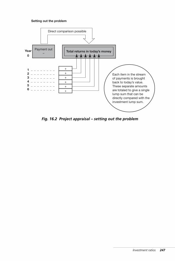
Investment ratios 247
Payment out–
123456
++++++
Each item in the streamof payments is broughtback to today’s value.These separate amountsare totaled to give a singlelump sum that can bedirectly compared with theinvestment lump sum.
Total returns in today’s money
Setting out the problem
Direct comparison possible
0
Year
Fig. 16.2 Project appraisal – setting out the problem
WKMR_CH16.QXD 11/24/05 12:46 PM Page 247
248 Key management ratios
Project appraisal – steps to a solution (2)
The discount factor
We can approach this question by asking the question ‘If I had $100 avail-able for deposit in the bank at an interest rate of 10 percent, what wouldit be worth one year from now?’ The answer is of course $110.
Therefore $100 is the present value of $110 due in year 1 at a rate of10 percent (expressed as a decimal = 0.1). We can bring any value backfrom the future to the present by applying a factor related to the interestrate. In this case we divide the future value by (1 + decimal interest rate),i.e. $110/ 1.1 = $100. (It is mathematically identical to multiply bythe discount factor .909, i.e., 1/1.1.)
If the future cash flow was positioned in Period 2, then we would haveto do the calculation twice, i.e. 1––1.1 × 1––1.1 = .826. In reality we do not maketwo calculations, we apply a factor that has the equivalent effect.
Figure 16.3 illustrates the effect of taking the value of a present sum ofmoney either forward in time or back in time.
Centrally placed is the box showing $100 which is aligned with thePeriod 0. Periods going forward into the future and back into the past areshown on the right- and left-hand sides of zero respectively. An interestrate of 10 percent is used here to keep things simple. As we move to theright of the central zero point, the interest factors are 1.100, 1.210 and1.331, which is 10 percent compounded for years +1, +2 and +3.
When applied to the sum of $100 they tell us that the equivalent is$133.1 at the end of Year 3.
To the left of the model, the factors are 0.909, 0.826 and 0.751. Thislast one tells us that $100 carried back three years has a present valueof $75.1.
The investment appraisal technique relies mainly on the factors to theleft of center, i.e. the discount factors.
To carry out our analysis we first select an appropriate interest rate. Ahigher rate would give a lower discount factor and vice versa. (See appen-dix 4 for relevant interest rate tables.) We can calculate the present orfuture value of any sum of money due in any period past or future byusing such tables.
☛
%
As stated above, we know that money due in a future time period has less valuethan money in our hands today. But how much less?
?
WKMR_CH16.QXD 11/24/05 12:46 PM Page 248

Investment ratios 249
Assumed rate of interest10%
Go back in time Go forward in time
Cashequivalents
Interestfactors
$110.0
1.100
$121.0
1.210
$133.1
1.331
Years + 1 + 2 + 3$100
These values are not oftenused in this application exceptin some theroretical exercises.
These values are of greatinterest to us. We use theinterest factors to calculatethe present value of futurepayments, for thepurpose shown above.
To bring a payment backthree years at 10%, multiplyby the factor 0.751.
Cashequivalents
Interestfactors
$75.1
0.751
$82.6
0.826
$90.9
0.909
Years–1–2–3
Fig. 16.3 Project appraisal – effects of time on value of a cash flow
WKMR_CH16.QXD 11/24/05 12:46 PM Page 249
250 Key management ratios
Project appraisal – present value (PV)
Figure 16.4 shows an example of a three-year project:
Investment $5,000
Return in: Year 1 $1,500Year 2 $3,500Year 3 $1,400
We wish to ascertain if the rate of return on this investment is greater orless than 10 percent.
In figure 16.2, we saw the method for setting out the problem; figure16.4 shows how the 10 percent discount factors are applied to the streamof returns. Each future payment is connected by an arrow back to thepresent time, showing the conversion of future cash flows into present-day values. The discount factor for one year at 10 percent is 0.909, for twoyears it is 0.826, etc.
The present value of each conversion is shown, i.e., $1,364 for year 1,etc. All individual present values are summed to give a total $5,309. Thetechnical name for this amount of $5,309 is the present value (PV) ofthe project’s future cash flows.
This sum can now be directly compared with the initial investment of$5,000. Cash in-flows are shown positive and out-flows negative. The posi-tive sum of $5,309 is offset against the negative sum of $5,000 to give anet present value (NPV) of $309 (positive).
What information can be drawn from the NPV? Figure 16.5 will help us to inter-pret the result.
?
%
WKMR_CH16.QXD 11/24/05 12:46 PM Page 250
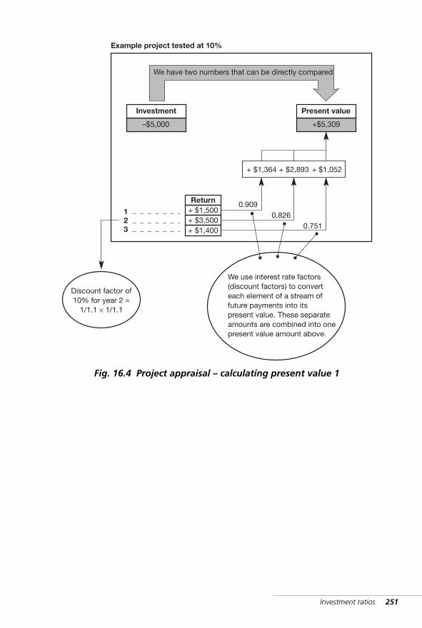
Investment ratios 251
–$5,000
123
Return+ $1,500+ $3,500+ $1,400
+ $1,364
0.909
We have two numbers that can be directly compared
+ $2,893 + $1,052
0.8260.751
Investment
+$5,309
Present value
We use interest rate factors(discount factors) to converteach element of a stream offuture payments into itspresent value. These separateamounts are combined into onepresent value amount above.
Example project tested at 10%
Discount factor of10% for year 2 =
1/1.1 × 1/1.1
Fig. 16.4 Project appraisal – calculating present value 1
WKMR_CH16.QXD 11/24/05 12:46 PM Page 251
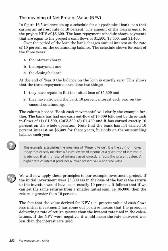
252 Key management ratios
The meaning of Net Present Value (NPV)
In figure 16.5 we have set up a schedule for a hypothetical bank loan thatcarries an interest rate of 10 percent. The amount of the loan is equal tothe project NPV of $5,309. The loan repayment schedule shows paymentsthat are equal to the project’s cash flows of $1,500, $3,500, and $1,400.
Over the period of the loan the bank charges annual interest at the rateof 10 percent on the outstanding balance. The schedule shows for each ofthe three years:
a the interest charge
b the repayment and
c the closing balance.
At the end of Year 3 the balance on the loan is exactly zero. This showsthat the three repayments have done two things:
1. they have repaid in full the initial loan of $5,309 and
2. they have also paid the bank 10 percent interest each year on theamount outstanding.
The column headed ‘Bank cash movements’ will clarify the example fur-ther. The bank has had one cash out-flow of $5,309 followed by three cashin-flows of (1) $1,500, (2)$3,500 (3) $1,400 and it has earned exactly 10percent on the whole operation. Note that the bank has not earned 10percent interest on $5,309 for three years, but only on the outstandingbalance each year.
We will now apply these principles to our example investment project. Ifthe initial investment were $5,309 (as in the case of the bank) the returnto the investor would have been exactly 10 percent. It follows that if wecan get the same returns from a smaller initial sum, i.e. $5,000, then thereturn is greater than 10 percent.
The fact that the value derived for NPV (i.e. present value of cash flowsless initial investment) has come out positive means that the project isdelivering a rate of return greater than the interest rate used in the calcu-lations. If the NPV were negative, it would mean the rate delivered wasless than the interest rate used.
This example establishes the meaning of ‘Present Value’. It is the sum of moneytoday that exactly matches a future stream of income at a given rate of interest. Itis obvious that the rate of interest used directly affects the present value. Ahigher rate of interest produces a lower present value and vice versa.
?
%
WKMR_CH16.QXD 11/24/05 12:46 PM Page 252
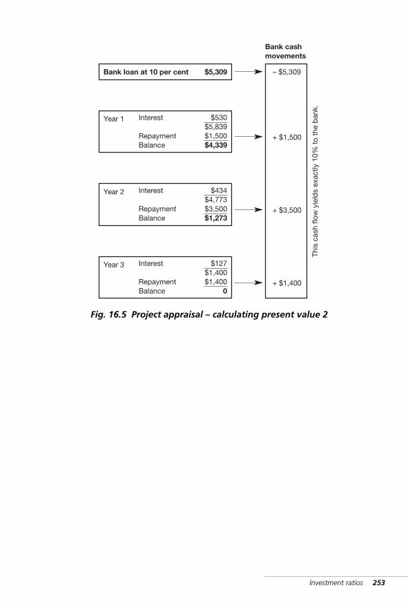
Investment ratios 253
Bank loan at 10 per cent
Year 1 Interest
RepaymentBalance
$530$5,839$1,500$4,339
$5,309
Year 2 Interest
RepaymentBalance
$434$4,773$3,500$1,273
Year 3 Interest
RepaymentBalance
$127$1,400$1,400
0
+ $1,500
– $5,309
+ $3,500
+ $1,400
This
cas
h flo
w y
ield
s ex
actly
10%
to
the
ban
k.
Bank cashmovements
Fig. 16.5 Project appraisal – calculating present value 2
WKMR_CH16.QXD 11/24/05 12:46 PM Page 253
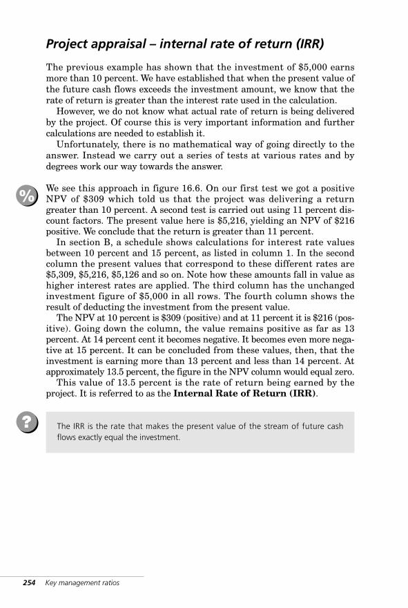
254 Key management ratios
Project appraisal – internal rate of return (IRR)
The previous example has shown that the investment of $5,000 earnsmore than 10 percent. We have established that when the present value ofthe future cash flows exceeds the investment amount, we know that therate of return is greater than the interest rate used in the calculation.
However, we do not know what actual rate of return is being deliveredby the project. Of course this is very important information and furthercalculations are needed to establish it.
Unfortunately, there is no mathematical way of going directly to theanswer. Instead we carry out a series of tests at various rates and bydegrees work our way towards the answer.
We see this approach in figure 16.6. On our first test we got a positiveNPV of $309 which told us that the project was delivering a returngreater than 10 percent. A second test is carried out using 11 percent dis-count factors. The present value here is $5,216, yielding an NPV of $216positive. We conclude that the return is greater than 11 percent.
In section B, a schedule shows calculations for interest rate valuesbetween 10 percent and 15 percent, as listed in column 1. In the secondcolumn the present values that correspond to these different rates are$5,309, $5,216, $5,126 and so on. Note how these amounts fall in value ashigher interest rates are applied. The third column has the unchangedinvestment figure of $5,000 in all rows. The fourth column shows theresult of deducting the investment from the present value.
The NPV at 10 percent is $309 (positive) and at 11 percent it is $216 (pos-itive). Going down the column, the value remains positive as far as 13percent. At 14 percent cent it becomes negative. It becomes even more nega-tive at 15 percent. It can be concluded from these values, then, that theinvestment is earning more than 13 percent and less than 14 percent. Atapproximately 13.5 percent, the figure in the NPV column would equal zero.
This value of 13.5 percent is the rate of return being earned by theproject. It is referred to as the Internal Rate of Return (IRR).
The IRR is the rate that makes the present value of the stream of future cashflows exactly equal the investment.
?
%
WKMR_CH16.QXD 11/24/05 12:46 PM Page 254
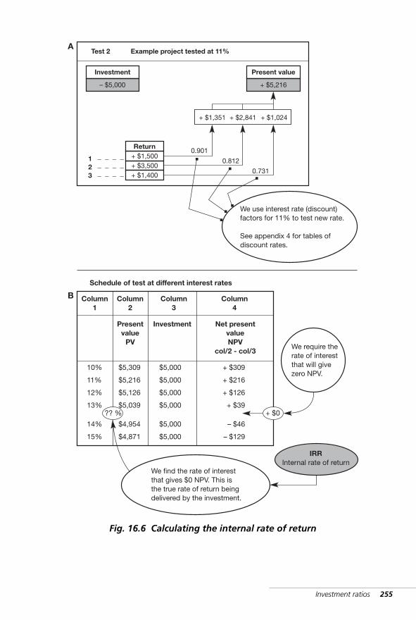
Investment ratios 255
– $5,000
123
Return+ $1,500+ $3,500+ $1,400
+ $1,351
0.901
ATest 2 Example project tested at 11%
+ $2,841 + $1,024
0.812
0.731
Investment
+ $5,216
Present value
We use interest rate (discount)factors for 11% to test new rate.
See appendix 4 for tables ofdiscount rates.
B
Presentvalue
PV
Investment Net presentvalueNPV
col/2 - col/3
10%
11%
12%
13%
14%
15%
$5,309
$5,216
$5,126
$5,039
$4,954
$4,871
$5,000
$5,000
$5,000
$5,000
$5,000
$5,000
+ $309
+ $216
+ $126
+ $39
– $46
– $129
Schedule of test at different interest rates
We find the rate of interestthat gives $0 NPV. This isthe true rate of return beingdelivered by the investment.
We require therate of interestthat will givezero NPV.
IRRInternal rate of return
+ $0?? %
Column1
Column2
Column3
Column4
Fig. 16.6 Calculating the internal rate of return
WKMR_CH16.QXD 11/24/05 12:46 PM Page 255
Project appraisal – summary
The method of investment appraisal that has been described is called thediscounted cash flow (DCF) technique. (see figure 16.7). To apply thistechnique the cash flow, positive or negative, for each time period mustfirst be identified. Then one or both of the approaches illustrated is used:
The NPV (net present value) method
■ select the required rate of interest (see below) ■ apply it to the stream of cash flows to derive net present value ■ if net present value is positive, select the project, otherwise do not.
The IRR (internal rate of return) method
■ find the interest rate that makes net present value equal to zero■ if this rate is satisfactory, select project, otherwise do not.
In this chapter we have merely considered how to apply a mathematicaltechnique once the cash flows from a project have been established.
In real life this is the easy part of project appraisal. It requires consider-ably more effort and skill to arrive at the expected cash flows. Furthermoremanagers will never have to physically do the calculations themselvesbecause computer programs are available to do this for them. However, amanager must understand the reasoning behind the calculations so that hecan formulate a problem correctly and interpret the results produced bythe computer. The various ratios produced by these programs can help himto make sound decisions in the field of investment appraisal.
Figure 16.7 gives an outline structure for of the inputs that are requiredto analyze an investment decision. These inputs can be grouped underfour headings:
■ cost of investment■ annual returns from project■ life of project ■ rate of interest.
A brief description of each is given. The area for which it is hardest toinput reliable data is that of ‘annual returns’. There are no rules for this.Common sense and business acumen must apply here. It is normal to testa series of scenarios to examine the sensitivity of the project to smallchanges in input variables. Over time the accuracy of predictions can bemonitored and suitable filtering mechanisms adopted.
256 Key management ratios
☛
✓
WKMR_CH16.QXD 11/24/05 12:46 PM Page 256
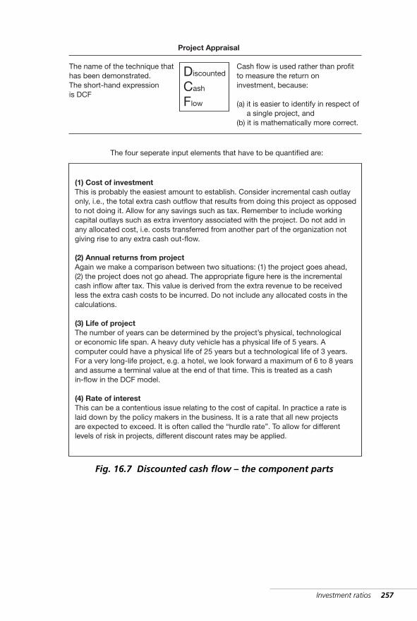
Investment ratios 257
The name of the technique thathas been demonstrated.The short-hand expressionis DCF
Cash flow is used rather than profitto measure the return oninvestment, because:
(a) it is easier to identify in respect of(a) a single project, and(b) it is mathematically more correct.
Discounted
Cash
Flow
Project Appraisal
(1) Cost of investmentThis is probably the easiest amount to establish. Consider incremental cash outlayonly, i.e., the total extra cash outflow that results from doing this project as opposedto not doing it. Allow for any savings such as tax. Remember to include workingcapital outlays such as extra inventory associated with the project. Do not add inany allocated cost, i.e. costs transferred from another part of the organization notgiving rise to any extra cash out-flow.
(2) Annual returns from projectAgain we make a comparison between two situations: (1) the project goes ahead,(2) the project does not go ahead. The appropriate figure here is the incrementalcash inflow after tax. This value is derived from the extra revenue to be receivedless the extra cash costs to be incurred. Do not include any allocated costs in thecalculations.
(3) Life of projectThe number of years can be determined by the project’s physical, technologicalor economic life span. A heavy duty vehicle has a physical life of 5 years. Acomputer could have a physical life of 25 years but a technological life of 3 years.For a very long-life project, e.g. a hotel, we look forward a maximum of 6 to 8 yearsand assume a terminal value at the end of that time. This is treated as a cashin-flow in the DCF model.
(4) Rate of interestThis can be a contentious issue relating to the cost of capital. In practice a rate islaid down by the policy makers in the business. It is a rate that all new projectsare expected to exceed. It is often called the “hurdle rate”. To allow for different������������������ �������������������������������������������
The four seperate input elements that have to be quantified are:
Fig. 16.7 Discounted cash flow – the component parts
WKMR_CH16.QXD 11/24/05 12:46 PM Page 257

WKMR_CH16.QXD 11/24/05 12:46 PM Page 258
17 Shareholdervalue added(SVA)Introduction · Description
· Approach to valuation (1)
· Approach to valuation (2) · Value
for the equity shareholders
· Discount factor · Terminal
(continuing) value · Complete model
Capital, in the sense of capital value, issimply future income discounted or, inother words, capitalised.IRVING FISHER (1867–1947)
WKMR_CH17.QXD 11/24/05 2:57 PM Page 259

WKMR_CH17.QXD 11/24/05 2:57 PM Page 260

Shareholder value added (SVA) 261
Introduction
In chapter 12 we looked at various stockmarket ratios and traditionalapproaches to the measurement of corporate performance and value.These have been in use for many years, they are still widely used and theyhave served the business community well. However many practitionershave now come to the conclusion that something more is needed.
Global competition, worldwide recession, and complex financial instru-ments have shown up weaknesses in these traditional approaches. Thishas given rise to a search for more precise instruments of assessment.The search has not been in vain, and there are now exciting new develop-ments in this area.
The most robust of these new techniques is that most commonlyknown as ‘shareholder value added’ (SVA)*, but the terms ‘economicvalue added’ (EVA), and ‘market value added’ (MVA) are also used.
These systems all have the same underlying approach. They adopt aneconomic rather than an accounting stance, and they look to the futurerather than the past.
One of the problems with the purely accounting approach is that it relieslargely on values that are historic. Furthermore these values are derivedfrom accounting statements that are produced according to variousaccounting conventions. Often these conventions are more useful for audit-ing purposes rather than for performance assessment or valuation.
There are other issues that traditional approaches do not address explic-itly such as risk measurement and future capital investment. There is nodoubt that SVA methods provide a more comprehensive and philosophi-cally sound basis for managerial decisions than those used in the past.
* Dr Alfred Rappaport (author of Creating Shareholder Value) is one of the founders of themovement and the ideas in this chapter owe much to his initiatives.
WKMR_CH17.QXD 11/24/05 2:57 PM Page 261
Description
The economic viewpoint is that value is determined by future cash flowsrather than historic profit or balance sheet calculations. Cash is investedtoday in order to get a surplus back in the future. This future cash flowmust fully repay the initial investment and also cover the cost of thefunds over the period of investment. This cash flow technique has beenused for many years in the assessment of capital projects (see chapter 16).
Let us say that we are faced with a capital project decision on whether weshould spend $1m on a particular piece of equipment. We estimate futurerevenues and costs over the life of the equipment. We convert these intothe extra cash in-flow that the equipment will produce. We combine thatin-flow with other cash movements arising from working capital etc.Then we discount the total cash flow back to a net present value (NPV).We use that figure to assess the financial value of the investment.
The shareholder value approach is to use the same technique to assess thevalue of a company’s operations either in whole or in part.
However in regard to a company special considerations apply:
1. The returns from a company cannot be so neatly packaged as thosefrom a single piece of equipment. In a company there will be manydifferent operations each giving rise to a separate cash flow.
2. With a single piece of equipment there is usually a very definite andlimited life span, but not so with a company.
3. In straightforward project appraisal, a very pragmatic approach tothe selection of a discount factor is common. But what discountfactor should be applied to the cash flows of a company overall?This is a very important consideration because the factor chosenwill have a major bearing on the assessment.
4. Companies can be funded in many different ways. Various mixturesof equity and loan capital are used. How can these differences beaccommodated?
It is these issues that will be explored in the following pages. We will usethe SVA Sample Company Inc. shown in figure 17.1 to illustrate the discussion.
262 Key management ratios
✓
%
WKMR_CH17.QXD 11/24/05 2:57 PM Page 262
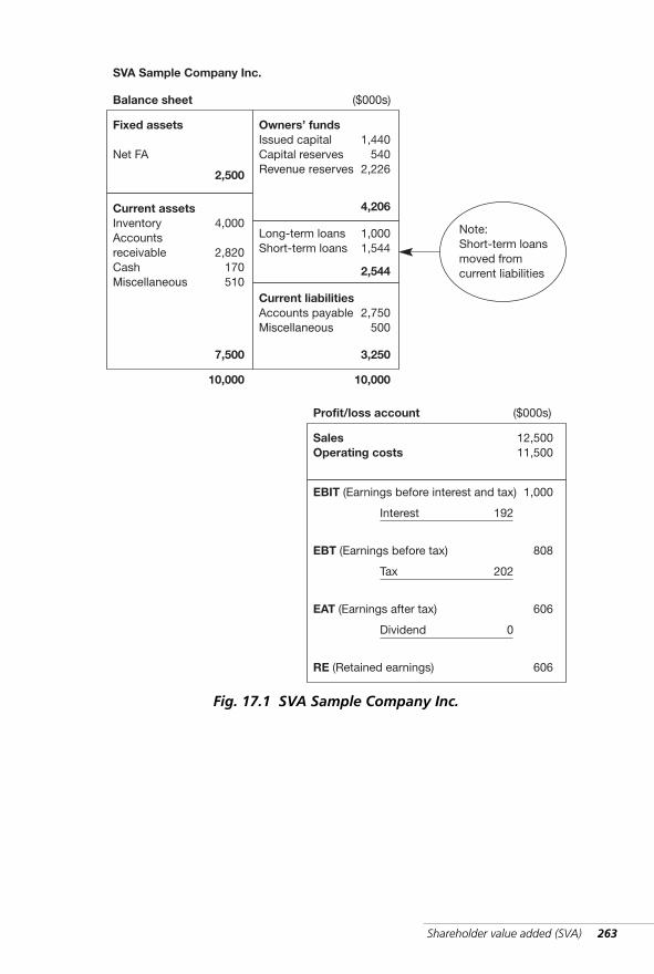
Shareholder value added (SVA) 263
EBIT (Earnings before interest and tax) 1,000
Interest 192
EBT (Earnings before tax) 808
Tax 202
EAT (Earnings after tax) 606
Dividend 0
RE (Retained earnings) 606
SalesOperating costs
12,50011,500
Profit/loss account ($000s)
Fixed assets
Net FA
Balance sheet ($000s)
2,500
Current assetsInventoryAccountsreceivableCashMiscellaneous
4,000
2,820170510
7,500
Owners’ fundsIssued capitalCapital reservesRevenue reserves
1,440540
2,226
4,206
Long-term loansShort-term loans
1,0001,544
2,544
Current liabilitiesAccounts payableMiscellaneous
2,750500
3,250
SVA Sample Company Inc.
Note:Short-term loansmoved fromcurrent liabilities
10,000 10,000
Fig. 17.1 SVA Sample Company Inc.
WKMR_CH17.QXD 11/24/05 2:57 PM Page 263
264 Key management ratios
Operating assets
Our first exercise is to re-arrange the balance sheet to separate out thenet operating assets i.e. those assets that are fundamental to the opera-tion of the business.* Figure 17.2 illustrates this.
* There may be assets in the balance sheet that are not essential to theexisting operations, e.g. surplus cash holdings. This matter will be dealtwith later.
There are three separate components:
1. Fixed assets $2,500
2. Current assets $7,500
3. Current liabilities * $3,250
* Observant readers will have noted that there are no short-term loans included in current liabil-ities. These loans are treated as part of the funding of the business for reasons to be seen shortly.
‘Current assets’ and ‘current liabilities’ are netted off to yield a figure for ‘networking capital’ (NWC) of $4,250. Accordingly, the net operating assets are:
1. Fixed assets $2,500
2. Net working capital $4,250
The funds in the balance sheet that match these operating assets we referto as ‘invested capital’ (IC).
For this exercise we will assume that all of the items included in oper-ating assets will respond spontaneously to changes in sales volume.
This assumption is reasonable for items in the ‘net working capital’ cate-gory. There is a direct linear relationship between ‘Accounts receivable’ andthe level of sales. So also with inventory, even though the link is not soclose. The same may be said of ‘Accounts payable’ on the liabilities side ofthe balance sheet. These are the three principal items in the NWC category.
In the case of ‘Cash’ we distinguish between the basic amount requiredfor operating requirements and surpluses held for other purposes. Thisbasic operating amount is a very small percentage of total assets and itcan be loosely linked to volume of activity.
For a comment on the relationship between ‘fixed assets’ and sales seethe following section.
%
WKMR_CH17.QXD 11/24/05 2:57 PM Page 264

Shareholder value added (SVA) 265
Current assetsCurrent liabilities
Net working capital(NWC)
7,500(3,250)
4,250
Fixed assets 2,500
Fixed assets
Net FA
Balance sheet ($000s)
2,500
Current assetsInventoryAccountsreceivableCash
4,000
3,330170
7,500
Owners’ fundsIssued capitalCapital reservesRevenue reserves
1,440540
2,226
4,206
Long-term loansShort-term loans
1,0001,544
2,544
Current liabilitiesAccounts payable 3,250
3,250
10,000 10,000
Operating assets 6,750
Operatingassets ($000s)
FA
NWC
2,500
4,250
6,750
Owners’funds
Long-termloansShort-termloans
4,206
1,000
1,544
6,750
Investedcapital
Fig. 17.2 Identify operating assets/funds
WKMR_CH17.QXD 11/24/05 2:57 PM Page 265
266 Key management ratios
Approach to valuation (1)
Forecast assumptions
Having identified the net operating assets, we will set about estimatingthe value of this company as determined by its expected future cash flowsand the discount factor to be applied to these.
We will illustrate this for our example company using some very simpleassumptions, such as a constant growth in sales of 10 percent.
There will be two main components to the cash flow:
1. Operating profits after tax
2. Cash flows arising from movements in assets.
The first of these is normally positive (cash in-flow) and the second nega-tive (cash out-flow). We have seen in chapter 14 that an increase in assetsgives rise to a cash out-flow. If assets are currently fully utilized, the extravolume of sales will probably require extra assets in support.
We must make some assumptions about the future operations. These are:
1. Growth in future sales 10 percent p.a.
2. Period of forecast four years
3. Margin on sales 8 percent
4. Tax rate 25 percent
5. Fixed assets required Linear to sales
6. Net working capital required Linear to sales
Figure 17.3 shows expected Sales, Fixed assets and Net working capitalamounts forecast for the next four years on an assumed growth rate of10 percent.
Note: We have suggested that there is strong justification for assuming alinear relationship between ‘net working capital’ and sales. But it is notrealistic to assume that fixed assets will move exactly in line with sales in anyone year. However, over longer periods this assumption may hold true. We areusing a simplified example here. In a practical application much thoughtwould be given to assessing fixed asset and working capital requirements.
%
WKMR_CH17.QXD 11/24/05 2:57 PM Page 266
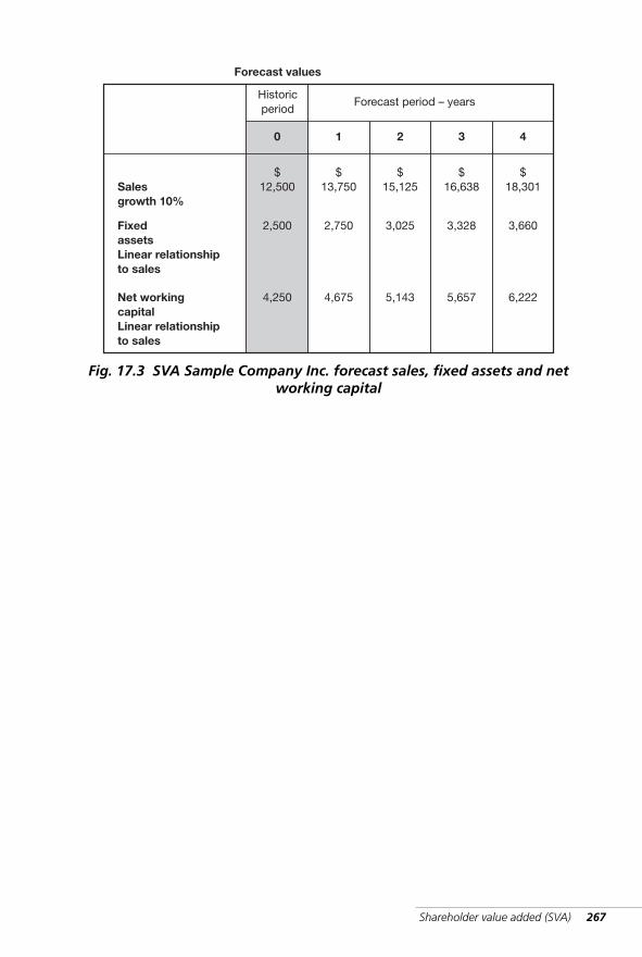
Shareholder value added (SVA) 267
Salesgrowth 10%
$12,500
$13,750
$15,125
$16,638
$18,301
FixedassetsLinear relationshipto sales
2,500 2,750 3,025 3,328 3,660
Net workingcapitalLinear relationshipto sales
4,250 4,675 5,143 5,657 6,222
0 1 2 3 4
Historicperiod
Forecast period – years
Forecast values
Fig. 17.3 SVA Sample Company Inc. forecast sales, fixed assets and networking capital
WKMR_CH17.QXD 11/24/05 2:57 PM Page 267
268 Key management ratios
Approach to valuation (2)
Forecast net cash flow
Figure 17.4 shows cash flow forecasts for the SVA Sample Company Inc.We take each of the three items forecast in the previous section and deriveits corresponding cash flow:
Section A: Cash flow forecasts
A.1 Sales with growth rate of 10 percent per annum.A.2 We apply the sales margin percentage (8 percent) to derive
operating profit. A.3 Tax is calculated at 25 percent and deducted.A.4 Net operating profit after tax (NOPAT). This is the figure we
take for the positive operating cash flows per annum that arisefrom trading.
Section B: Fixed assets:
B.2 The negative cash flow reflects the increase in value in FA each year.
Section C: Net working capital:
C.2 The negative cash flow reflects the increase in value of NWC each year.
Section D: Overall cash flow:
D.1 Cash flows from A, B, and C above are netted off to give values forexpected net cash flows for each of the next four years.
Depreciation and cash flow
However in our simple illustration, we ignore this adjustment both in theincome statement and again when we come to look at investment in fixed
Two questions immediately come to mind :
a What about the depreciation charged in the accounts? Should the forecastcash flows not be increased by a corresponding amount? and
b Why has tax been charged to profits before interest has been deducted?
Both of these questions will be dealt with below.
?
We know that cash flow from a trading operation can be defined as net profitplus depreciation. Should we not therefore add back depreciation to our cashflows? Strictly speaking, the answer is ‘yes’.
?
%
WKMR_CH17.QXD 11/24/05 2:57 PM Page 268
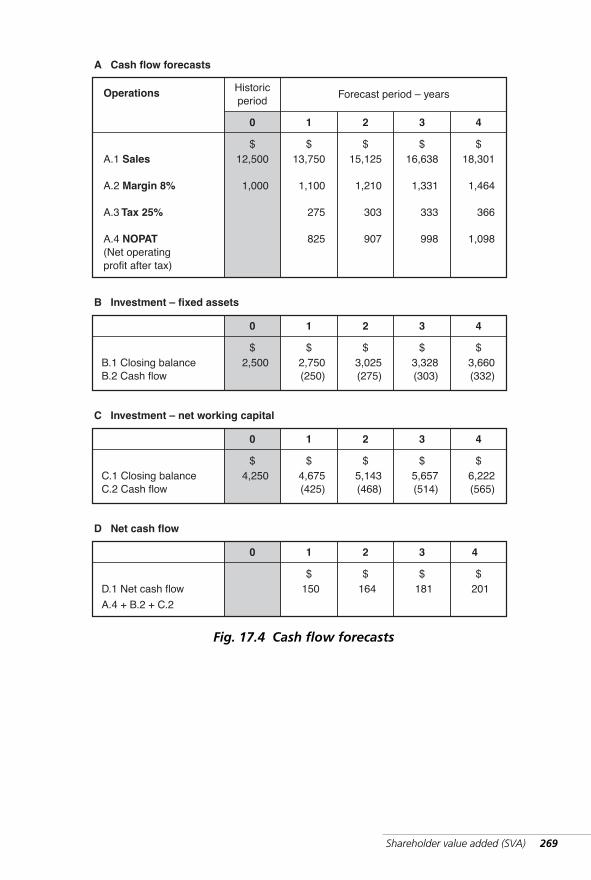
Shareholder value added (SVA) 269
$A.1 Sales
A.2 Margin 8%
A.3 Tax 25%
A.4 NOPAT(Net operatingprofit after tax)
12,500
1,000
13,750
1,100
275
825
15,125
1,210
303
907
16,638
1,331
333
998
18,301
1,464
366
1,098
0 1 2 3 4
Historicperiod
Forecast period – yearsOperations
$ $ $ $
A Cash flow forecasts
$B.1 Closing balanceB.2 Cash flow
2,500 2,750(250)
3,025(275)
3,328(303)
3,660(332)
0 1 2 3 4
$ $ $ $
B Investment – fixed assets
C.1 Closing balanceC.2 Cash flow
4,675(425)
5,143(468)
5,657(514)
6,222(565)
0 1 2 3 4
$ $ $ $
C Investment – net working capital
D.1 Net cash flow 150 164 181 201
0 1 2 3 4
$ $ $ $
D Net cash flow
4,250$
A.4 + B.2 + C.2
Fig. 17.4 Cash flow forecasts
WKMR_CH17.QXD 11/24/05 2:57 PM Page 269
270 Key management ratios
assets. In the latter case by taking only the net increase we ignore the invest-ment required to maintain a constant level of assets. This could be equatedto the depreciation charge. Consequently these two items cancel out.
Tax: We have charged tax at the full rate on operating profit. Would thisnot be shielded by our interest charge which would be deducted prior tothe tax charge? The reason for the treatment used here is that the ques-tion of funding is ignored. We can say that for the moment we areassuming that funding is entirely from equity.
Total present value
In figure 17.5 we perform three exercises:
■ We adopt a discount rate of 9.64 percent■ We discount the four-year cash flow back to period zero■ We decide on a ‘terminal value’ at year 4 and discount it back.
The present value of the first four years of operation amounts to $550.
Terminal value
This is perhaps the most important number in the whole equation.
There are many approaches and formulae used to estimate it, but in thissimple illustration we will assume that the company will have a marketvalue equal to ten times its ‘net operating profit after tax’ (NOPAT).
i.e., NOPAT (year 4) =$1,098Value at end of year 4 =$10,980 (NOPAT × 10)
This is the amount we could sell the company for at the end of year 4. Wecan therefore treat this figure as if it were a cash in-flow in that year. Weapply our discount rate of 9.64 percent to give a present value of $7,598,but see figure 17.13 for the revised method.
Likewise three important questions spring to mind at this stage:
■ Why use four years in preference to some other time period?
■ How do we decide on value remaining in the company at the end of whatevertime period we chose?
■ Why use 9.64 percent as our discount factor?
These crucial questions will all be addressed in detail in due course.
?
%
WKMR_CH17.QXD 11/24/05 2:57 PM Page 270
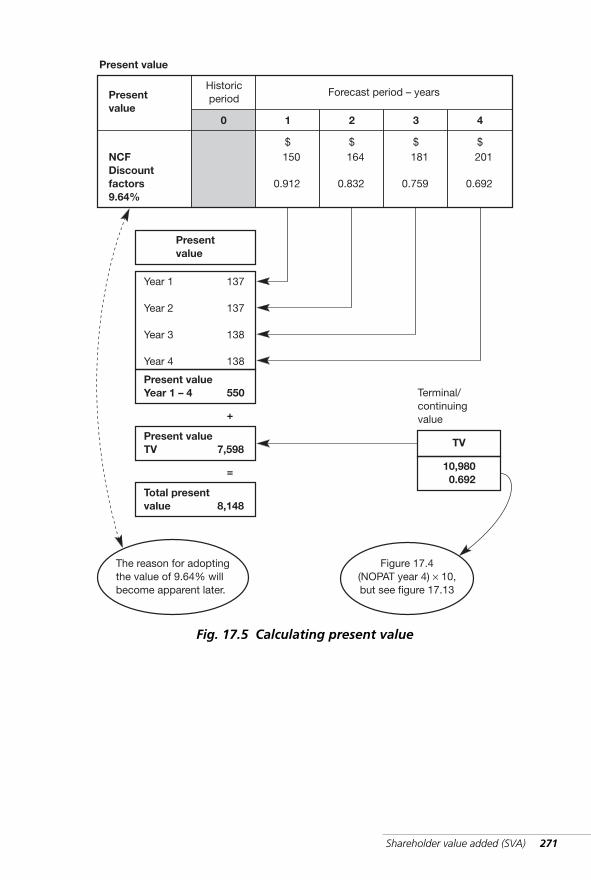
Shareholder value added (SVA) 271
NCFDiscountfactors9.64%
150
0.912
164
0.832
181
0.759
201
0.692
0 1 2 3 4
Historicperiod
Forecast period – yearsPresentvalue
$ $ $ $
Present value
Presentvalue
Year 1
Year 2
Year 3
Year 4
137
137
138
138
Present valueYear 1 – 4 550
Present valueTV 7,598
Total presentvalue 8,148
+
=
TV
10,9800.692
Terminal/continuingvalue
The reason for adoptingthe value of 9.64% willbecome apparent later.
Figure 17.4(NOPAT year 4) × 10,but see figure 17.13
Fig. 17.5 Calculating present value
WKMR_CH17.QXD 11/24/05 2:57 PM Page 271
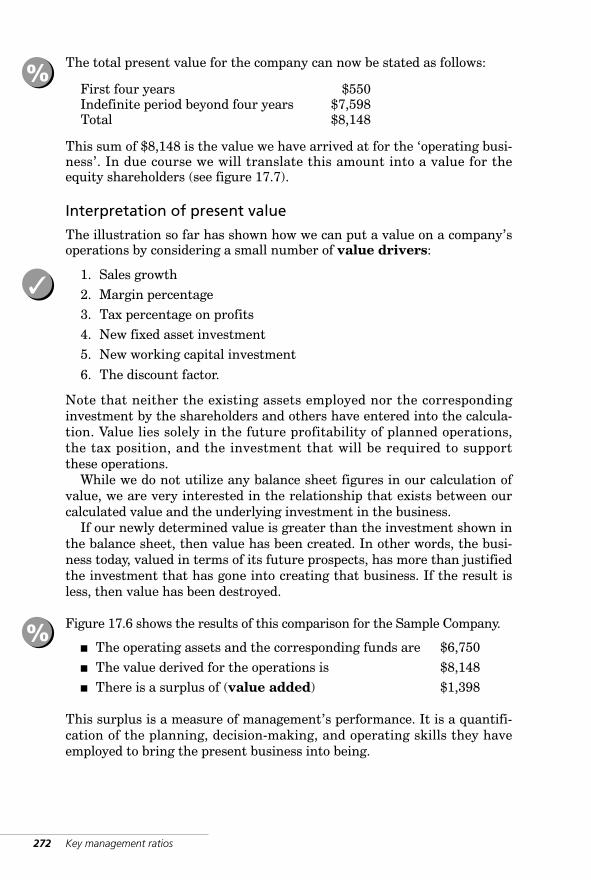
272 Key management ratios
The total present value for the company can now be stated as follows:
First four years $550Indefinite period beyond four years $7,598Total $8,148
This sum of $8,148 is the value we have arrived at for the ‘operating busi-ness’. In due course we will translate this amount into a value for theequity shareholders (see figure 17.7).
Interpretation of present value
The illustration so far has shown how we can put a value on a company’soperations by considering a small number of value drivers:
1. Sales growth2. Margin percentage3. Tax percentage on profits4. New fixed asset investment5. New working capital investment
6. The discount factor.
Note that neither the existing assets employed nor the correspondinginvestment by the shareholders and others have entered into the calcula-tion. Value lies solely in the future profitability of planned operations,the tax position, and the investment that will be required to supportthese operations.
While we do not utilize any balance sheet figures in our calculation ofvalue, we are very interested in the relationship that exists between ourcalculated value and the underlying investment in the business.
If our newly determined value is greater than the investment shown inthe balance sheet, then value has been created. In other words, the busi-ness today, valued in terms of its future prospects, has more than justifiedthe investment that has gone into creating that business. If the result isless, then value has been destroyed.
Figure 17.6 shows the results of this comparison for the Sample Company.
■ The operating assets and the corresponding funds are $6,750■ The value derived for the operations is $8,148■ There is a surplus of (value added) $1,398
This surplus is a measure of management’s performance. It is a quantifi-cation of the planning, decision-making, and operating skills they haveemployed to bring the present business into being.
%
%
✓
WKMR_CH17.QXD 11/24/05 2:57 PM Page 272
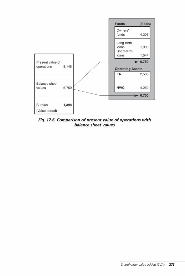
Shareholder value added (SVA) 273
($000s)Funds
Owners’funds
Long-termloansShort-termloans
4,206
1,000
1,544
6,750
Operating Assets
FA
NWC
2,500
4,250
6,750
Present value ofoperations
Balance sheetvalues
8,148
6,750
Surplus 1,398
(Value added)
Fig. 17.6 Comparison of present value of operations withbalance sheet values
WKMR_CH17.QXD 11/24/05 2:57 PM Page 273
274 Key management ratios
We can see what a powerful tool we have not only for decision-making,but for assessing and rewarding managerial performance.
Value for the equity shareholders
The calculated value of $8,148 relates to the operating business. We mustnow translate this into a value for the equity shareholders.
Two adjustments are required:
1. Non-operating assets
There may be assets in the balance sheet that are not essential to theexisting business. The most obvious case is where a company, for onereason or another, holds a large cash balance. It may be that the companyis planning future acquisitions.
The value of such assets must be added to that of the operations toarrive at the company value.
2. Non-equity funds
The equity shareholder stands at the end of the queue of those who pro-vide funds to a business. The claims of those who provide loan andpreference share capital have precedence.
All such prior claims must be deducted from the company value to arriveat the value for the equity shareholders.
SVA Sample CompanyIn figure 17.7 these calculations have been performed for the SampleCompany. Note that:
■ there are no non-operating assets in this case■ the total non-equity funds amount to $2,544 ■ the resulting equity value is $5,604.
The equity investment in the balance sheet amounts to $4,206, so the sur-plus is again $1,398. The total amount of the value added as a result ofgood management has accrued to the equity shareholders. Hence theterm ‘SVA’ (shareholder value added) that is given to this technique.
☛
%
WKMR_CH17.QXD 11/24/05 2:57 PM Page 274
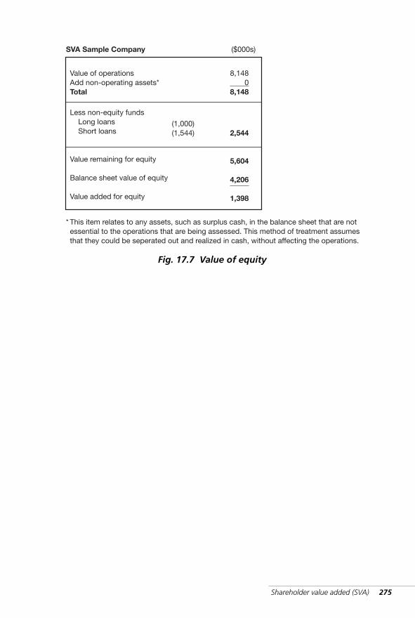
Shareholder value added (SVA) 275
8,1480
8,148
2,544
5,604
4,206
1,398
(1,000)(1,544)
($000s)SVA Sample Company
Value of operationsAdd non-operating assets*Total
Less non-equity funds Long loans Short loans
Value remaining for equity
Balance sheet value of equity
Value added for equity
* This item relates to any assets, such as surplus cash, in the balance sheet that are notessential to the operations that are being assessed. This method of treatment assumesthat they could be seperated out and realized in cash, without affecting the operations.
Fig. 17.7 Value of equity
WKMR_CH17.QXD 11/24/05 2:57 PM Page 275
276 Key management ratios
We use the technique not only to calculate a value for a particular oper-ating business, but also to compare and decide between alternativestrategies for a particular operation. Furthermore its particular strengthmay not even be to look at an overall business, but rather to identify whichof its component parts are adding value and which are destroying value.
In arriving at a value for the company we have skirted aroundsome very important matters:
■ The appropriate discount factor to be applied to the cash flows.■ The terminal value of the business, i.e. its continuing value
at the end of the forecast period.
Discount factor
All the funds used to support the business have a cost. This cost is obvious inthe case of loan funds. They carry a precise (but maybe varying) interest rateand their cost has always been charged against the profits of an operation.
In the case of common stock (equity) the cost is just as real but it hasnot always been so obvious. Indeed it is one of the main criticisms of moretraditional methods of assessment that this cost has not been made moreexplicit and charged against operations. In the SVA method of assessmentthe cost of equity is fully assessed and charged. The method employed isto use a discount factor based on the weighted average cost of capital.
Weighted average cost of capital (WACC)
Figure 17.8 shows the calculation.
■ We identify each source of funds and its corresponding cost. Somecosts, such as interest on loans, are tax deductible, other are not. Wemust therefore express all charges in constant after-tax terms. Forinstance if a loan carries a 10 percent coupon and the tax rate is 25percent, the after-tax cost is 8 percent.
■ We calculate for each source of funds its weighting, i.e. itspercentage of the total. For instance if total funds are $200 and wehave a loan of $50, we apply a weighting of 25 percent to that loan.
■ We multiply the cost of each source by its weighting to obtain itsweighted cost. The sum of all the weighted costs is WACC.
See important note (to figure 17.8) on the correct weights to use for calcu-lating WACC.
☛
WKMR_CH17.QXD 11/24/05 2:57 PM Page 276
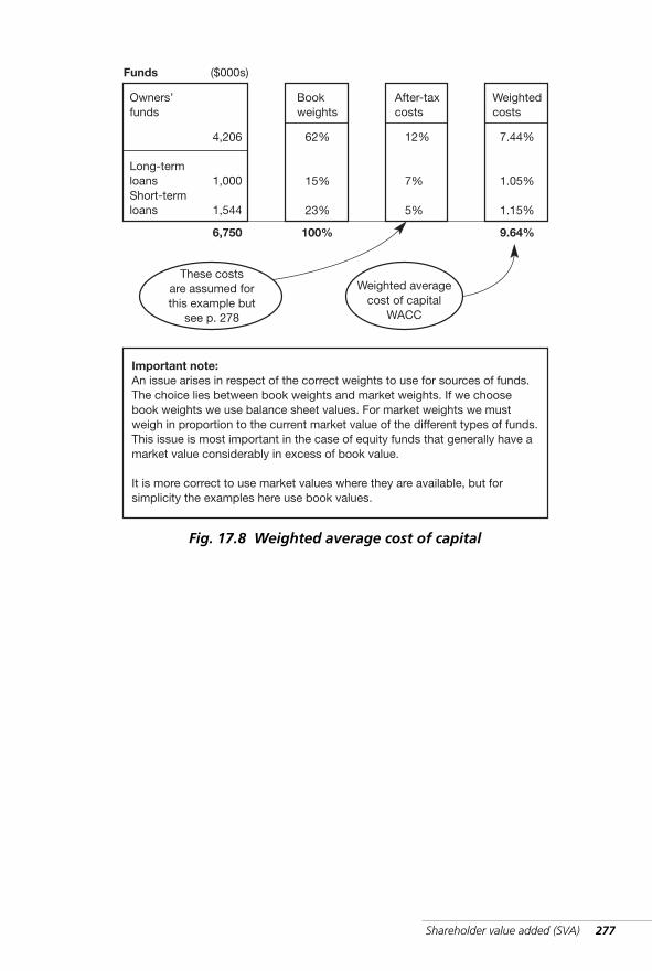
Shareholder value added (SVA) 277
($000s)Funds
Owners’funds
Long-termloansShort-termloans
4,206
1,000
1,544
6,750
Bookweights
62%
15%
23%
100%
After-taxcosts
12%
7%
5%
Weightedcosts
7.44%
1.05%
1.15%
9.64%
Important note:An issue arises in respect of the correct weights to use for sources of funds.The choice lies between book weights and market weights. If we choosebook weights we use balance sheet values. For market weights we mustweigh in proportion to the current market value of the different types of funds.This issue is most important in the case of equity funds that generally have amarket value considerably in excess of book value.
It is more correct to use market values where they are available, but forsimplicity the examples here use book values.
Weighted averagecost of capital
WACC
These costsare assumed forthis example but
see p. 278
Fig. 17.8 Weighted average cost of capital
WKMR_CH17.QXD 11/24/05 2:57 PM Page 277
278 Key management ratios
The cost of equity capital
The cost of loan capital is simply the after-tax interest cost. The cost ofcommon equity is not so easy to establish. It is an issue that has exercisedmany eminent minds over a number of decades.
The problem is that the cost of equity is not based on a contract but onthe expectations.
The assessment of expected return will be based on the investor’s view ofthe following benefits (see figure 17.9):
■ The stream of annual dividends■ The growth in the share market price.
The degree of confidence will be a function of the perceived risk of theinvestment. The investor knows that risk is inherent in business. He/shedoes not like to take risks and he/she will have to be rewarded for doing so.The higher the perceived risk the greater the return he/she will require.
The investor has a wide range of opportunities for investment. Thesecan be classified into low-risk investments yielding relatively low returns,e.g., government securities, and higher-risk investments that must offerthe promise of higher returns. Equity shares fall into this latter category.
Because we are dealing with estimates that exist in the minds of thou-sands of investors it is very difficult to quantify these factors. All we cando is to observe behavior in the market-place and try to construct modelsto explain that behavior.
The cost of equity to the company is the overall rate of return it must promise todeliver to the investor to persuade him/her to invest. It can also be expressed asthe amount an extra unit of equity brought into the company must earn in ordernot to dilute the return to the existing shareholders.
In order to ascertain this cost of equity the two great imponderables are:
■ growth from an existing position
■ risk.
?
When the equity shareholder invests he/she does so on the basis of two estimates:
■ What return can I expect?
■ What degree of confidence can I have in this expectation?
?
WKMR_CH17.QXD 11/24/05 2:57 PM Page 278
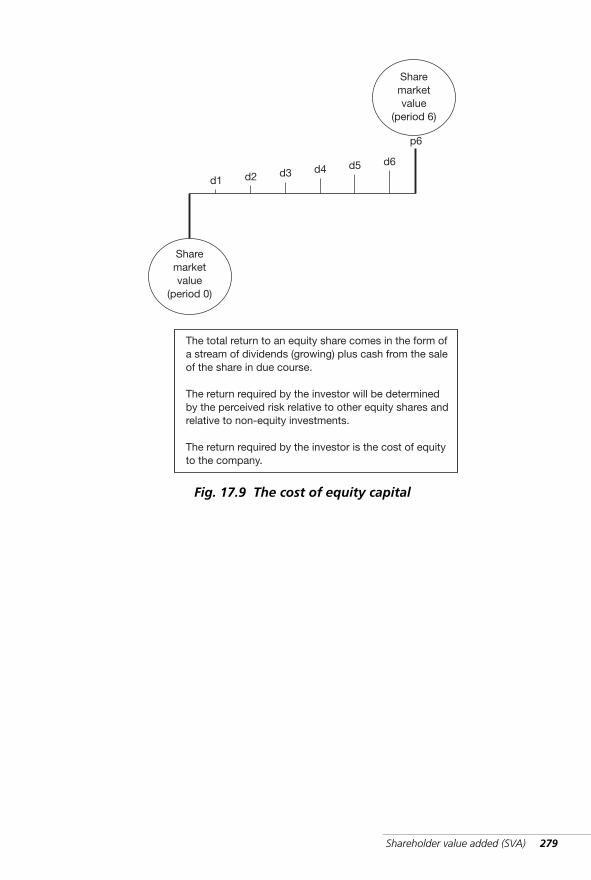
Shareholder value added (SVA) 279
p6
Sharemarketvalue
(period 0)
Sharemarketvalue
(period 6)
The total return to an equity share comes in the form ofa stream of dividends (growing) plus cash from the saleof the share in due course.
The return required by the investor will be determinedby the perceived risk relative to other equity shares andrelative to non-equity investments.
The return required by the investor is the cost of equityto the company.
d5 d6d4d3d2d1
Fig. 17.9 The cost of equity capital
WKMR_CH17.QXD 11/24/05 2:57 PM Page 279
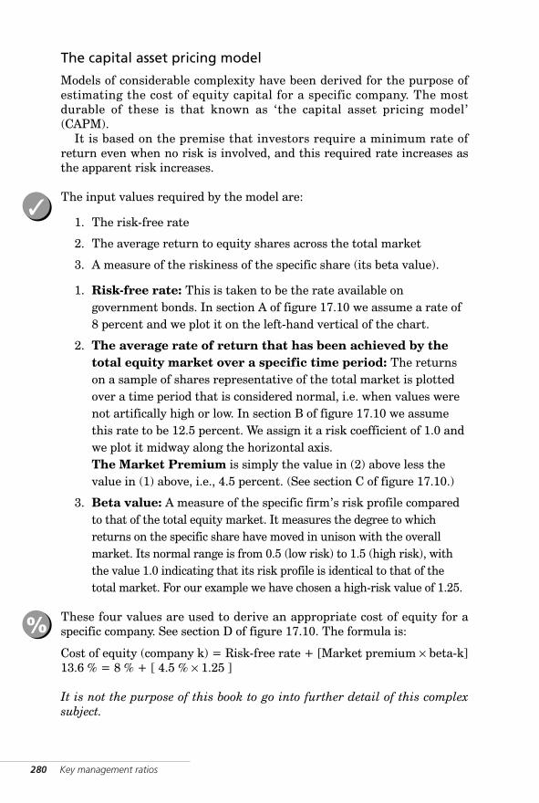
280 Key management ratios
The capital asset pricing model
Models of considerable complexity have been derived for the purpose ofestimating the cost of equity capital for a specific company. The mostdurable of these is that known as ‘the capital asset pricing model’(CAPM).
It is based on the premise that investors require a minimum rate ofreturn even when no risk is involved, and this required rate increases asthe apparent risk increases.
The input values required by the model are:
1. The risk-free rate
2. The average return to equity shares across the total market
3. A measure of the riskiness of the specific share (its beta value).
1. Risk-free rate: This is taken to be the rate available ongovernment bonds. In section A of figure 17.10 we assume a rate of8 percent and we plot it on the left-hand vertical of the chart.
2. The average rate of return that has been achieved by thetotal equity market over a specific time period: The returnson a sample of shares representative of the total market is plottedover a time period that is considered normal, i.e. when values werenot artifically high or low. In section B of figure 17.10 we assumethis rate to be 12.5 percent. We assign it a risk coefficient of 1.0 andwe plot it midway along the horizontal axis.The Market Premium is simply the value in (2) above less thevalue in (1) above, i.e., 4.5 percent. (See section C of figure 17.10.)
3. Beta value: A measure of the specific firm’s risk profile comparedto that of the total equity market. It measures the degree to whichreturns on the specific share have moved in unison with the overallmarket. Its normal range is from 0.5 (low risk) to 1.5 (high risk), withthe value 1.0 indicating that its risk profile is identical to that of thetotal market. For our example we have chosen a high-risk value of 1.25.
These four values are used to derive an appropriate cost of equity for aspecific company. See section D of figure 17.10. The formula is:
Cost of equity (company k) = Risk-free rate + [Market premium × beta-k]13.6 % = 8 % + [ 4.5 % × 1.25 ]
It is not the purpose of this book to go into further detail of this complexsubject.
%
✓
WKMR_CH17.QXD 11/24/05 2:57 PM Page 280
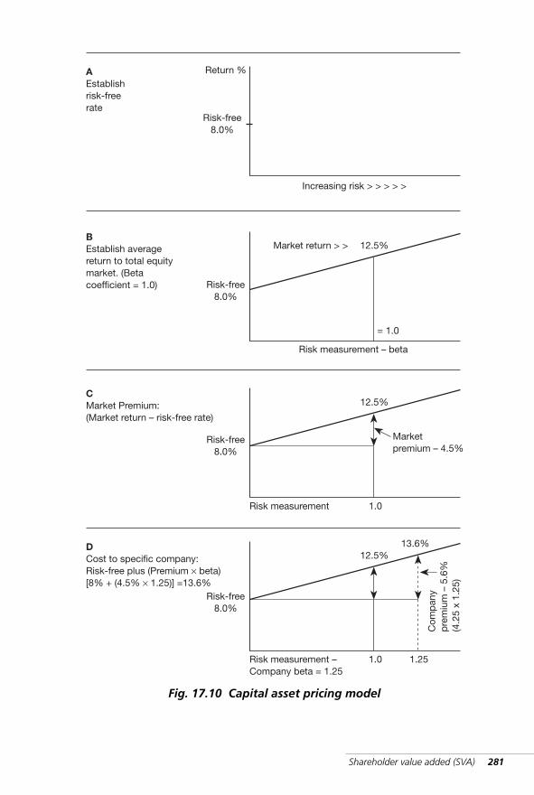
Shareholder value added (SVA) 281
Cost to specific company:Risk-free plus (Premium × beta)[8% + (4.5% × 1.25)] =13.6%
Risk measurement –Company beta = 1.25
Com
pan
yp
rem
ium
– 5
.6%
(4.2
5 x
1.25
)
1.0 1.25
12.5%13.6%
Market Premium:(Market return – risk-free rate)
Risk measurement
Marketpremium – 4.5%
1.0
12.5%
Establish averagereturn to total equitymarket. (Betacoefficient = 1.0) Risk-free
8.0%
Risk measurement – beta
12.5%
Establishrisk-freerate
Increasing risk > > > > >
Return %
Market return > >
D
C
B
A
= 1.0
Risk-free8.0%
Risk-free8.0%
Risk-free8.0%
Fig. 17.10 Capital asset pricing model
WKMR_CH17.QXD 11/24/05 2:57 PM Page 281
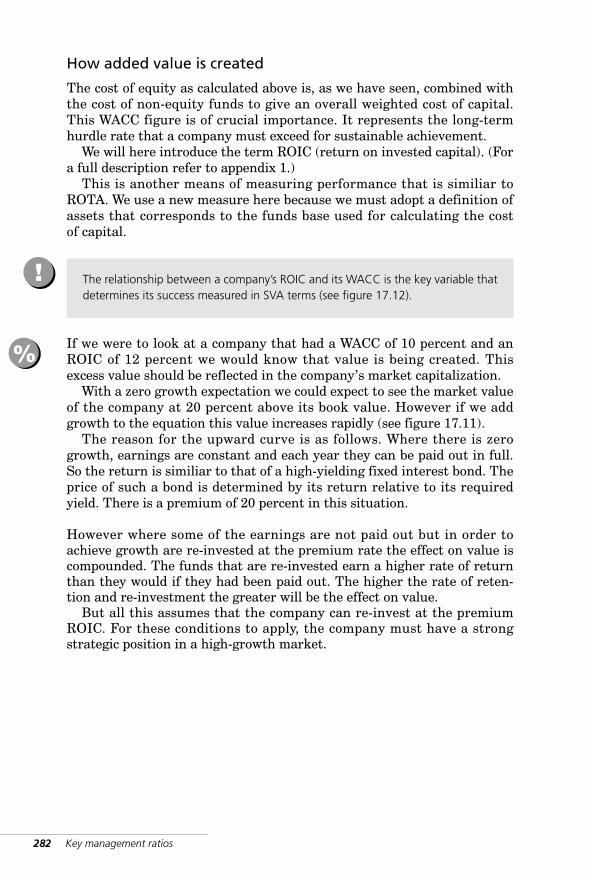
282 Key management ratios
How added value is created
The cost of equity as calculated above is, as we have seen, combined withthe cost of non-equity funds to give an overall weighted cost of capital.This WACC figure is of crucial importance. It represents the long-termhurdle rate that a company must exceed for sustainable achievement.
We will here introduce the term ROIC (return on invested capital). (Fora full description refer to appendix 1.)
This is another means of measuring performance that is similiar toROTA. We use a new measure here because we must adopt a definition ofassets that corresponds to the funds base used for calculating the costof capital.
If we were to look at a company that had a WACC of 10 percent and anROIC of 12 percent we would know that value is being created. Thisexcess value should be reflected in the company’s market capitalization.
With a zero growth expectation we could expect to see the market valueof the company at 20 percent above its book value. However if we addgrowth to the equation this value increases rapidly (see figure 17.11).
The reason for the upward curve is as follows. Where there is zerogrowth, earnings are constant and each year they can be paid out in full.So the return is similiar to that of a high-yielding fixed interest bond. Theprice of such a bond is determined by its return relative to its requiredyield. There is a premium of 20 percent in this situation.
However where some of the earnings are not paid out but in order toachieve growth are re-invested at the premium rate the effect on value iscompounded. The funds that are re-invested earn a higher rate of returnthan they would if they had been paid out. The higher the rate of reten-tion and re-investment the greater will be the effect on value.
But all this assumes that the company can re-invest at the premiumROIC. For these conditions to apply, the company must have a strongstrategic position in a high-growth market.
The relationship between a company’s ROIC and its WACC is the key variable thatdetermines its success measured in SVA terms (see figure 17.12).
!
%
WKMR_CH17.QXD 11/24/05 2:57 PM Page 282
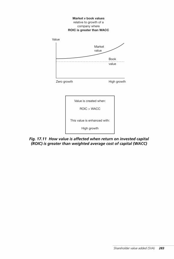
Shareholder value added (SVA) 283
Market v book valuesrelative to growth of a
company whereROIC is greater than WACC
Value
Zero growth
Marketvalue
High growth
Book
value
Value is created when:
ROIC > WACC
This value is enhanced with:
High growth
Fig. 17.11 How value is affected when return on invested capital(ROIC) is greater than weighted average cost of capital (WACC)
WKMR_CH17.QXD 11/24/05 2:57 PM Page 283
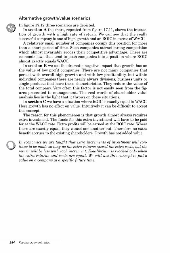
284 Key management ratios
Alternative growth/value scenarios
In figure 17.12 three scenarios are depicted. In section A the chart, repeated from figure 17.11, shows the interac-
tion of growth with a high rate of return. We can see that the reallysuccessful company is one of high growth and an ROIC in excess of WACC.
A relatively small number of companies occupy this position for morethan a short period of time. Such companies attract strong competitionwhich almost invariably erodes their competitive advantage. There areeconomic laws that tend to push companies into a position where ROICalmost exactly equals WACC.
In section B we see the dramatic negative impact that growth has onthe value of low profit companies. There are not many companies thatpersist with overall high growth and with low profitability, but withinindividual companies there are nearly always divisions, business units orsingle products that have these characteristics. They reduce the value ofthe total company. Very often this factor is not easily seen from the fig-ures presented to management. The real worth of shareholder valueanalysis lies in the light that it throws on these situations.
In section C we have a situation where ROIC is exactly equal to WACC.Here growth has no effect on value. Intuitively it can be difficult to acceptthis concept.
The reason for this phenomenon is that growth almost always requiresextra investment. The funds for this extra investment will have to be paidfor at the WACC rate. Extra profits will be earned at the ROIC rate. Wherethese are exactly equal, they cancel one another out. Therefore no extrabenefit accrues to the existing shareholders. Growth has not added value.
In economics we are taught that extra increments of investment will con-tinue to be made so long as the extra returns exceed the extra costs, but thereturn will be less with each increment. Equilibrium is reached only whenthe extra returns and costs are equal. We will use this concept to put avalue on a company at a specific future time.
%
WKMR_CH17.QXD 11/24/05 2:57 PM Page 284
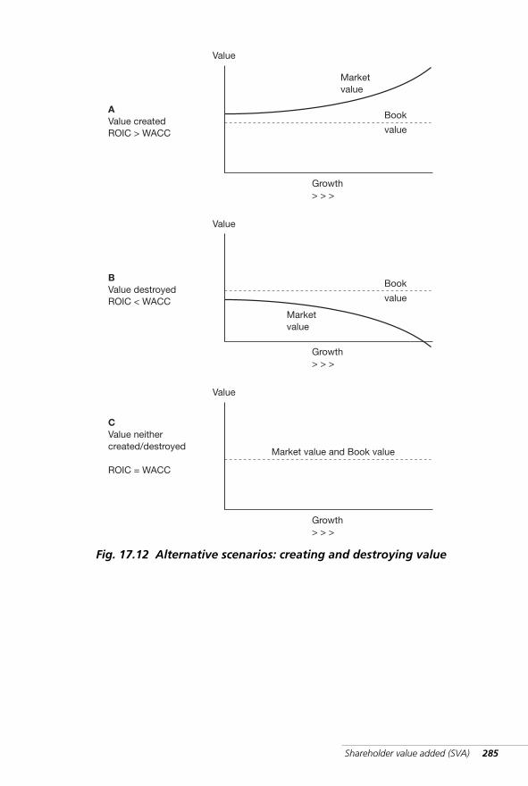
Shareholder value added (SVA) 285
Value
Growth> > >
Marketvalue
Book
value
AValue createdROIC > WACC
Value
Growth> > >
Marketvalue
Book
value
BValue destroyedROIC < WACC
Value
Growth> > >
Market value and Book value
CValue neithercreated/destroyed
ROIC = WACC
Fig. 17.12 Alternative scenarios: creating and destroying value
WKMR_CH17.QXD 11/24/05 2:57 PM Page 285
286 Key management ratios
Terminal (continuing) value
The second important issue we did not fully deal with is the question ofterminal value. We simply assumed this to be ten times the amount ofprofit in the final year.
We need a more soundly based approach than this. We will use the ROIC –WACC relationship to direct us towards a logical solution.
Management’s objective is to implement strategies that will give theircompany a competitive advantage that will allow it to earn a returngreater than WACC. Where they achieve this premium return they addvalue for the shareholders.
However this premium return will inevitably attract competition thatwill whittle away its advantage over time. Without some competitive advan-tage a company will not continue to earn premium profits, so its ROIC willfall back to the level of WACC. Of course, good management will continu-ously seek to put in place new strategies that will restore the advantage.
In shareholder value analysis we assess the number of years forward forwhich current strategies will continue to add value. At the end of that‘horizon period’ there will be equality between ROIC and WACC. Furthergrowth beyond that date will not add value. We make this the point wherewe assess the continuing or terminal value of the company.
To calculate the terminal value we simply take the cash flow in thatfinal year and assess it as we would value an annuity. That is we dividethe cash flow by the cost of capital. When we use this more logically soundapproach in our example we produce a value somewhat in excess of theearlier shortcut approach. See figure 17.13.
See appendix 1 for futher discussion of terminal value calculations.
The valuation approach we use here is one that measures the value of the com-pany as it now stands with its existing strategies.
!
☛
WKMR_CH17.QXD 11/24/05 2:57 PM Page 286
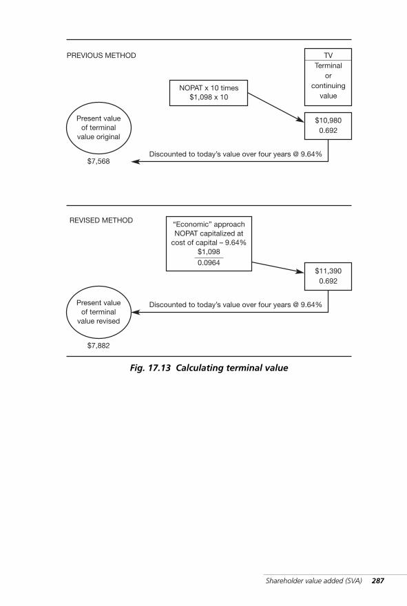
Shareholder value added (SVA) 287
NOPAT x 10 times$1,098 x 10
TVTerminal
orcontinuing
value
$10,9800.692
Present valueof terminal
value original
Discounted to today’s value over four years @ 9.64%
PREVIOUS METHOD
$7,568
“Economic” approachNOPAT capitalized at
cost of capital – 9.64%$1,098
0.0964$11,3900.692
Present valueof terminal
value revised
Discounted to today’s value over four years @ 9.64%
REVISED METHOD
$7,882
Fig. 17.13 Calculating terminal value
WKMR_CH17.QXD 11/24/05 2:57 PM Page 287
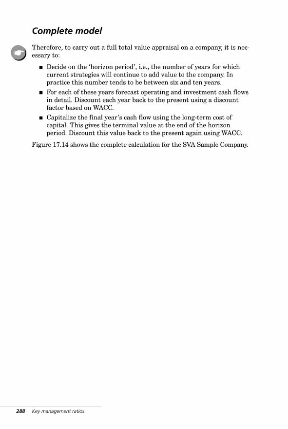
Complete model
Therefore, to carry out a full total value appraisal on a company, it is nec-essary to:
■ Decide on the ‘horizon period’, i.e., the number of years for whichcurrent strategies will continue to add value to the company. Inpractice this number tends to be between six and ten years.
■ For each of these years forecast operating and investment cash flowsin detail. Discount each year back to the present using a discountfactor based on WACC.
■ Capitalize the final year’s cash flow using the long-term cost ofcapital. This gives the terminal value at the end of the horizonperiod. Discount this value back to the present again using WACC.
Figure 17.14 shows the complete calculation for the SVA Sample Company.
288 Key management ratios
☛
WKMR_CH17.QXD 11/24/05 2:57 PM Page 288
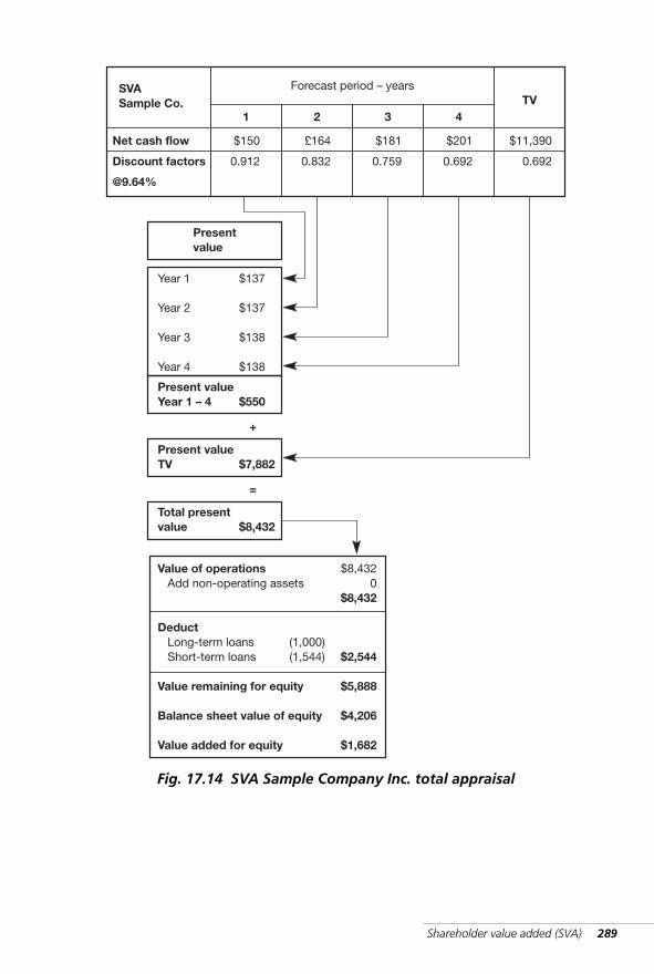
Shareholder value added (SVA) 289
Net cash flow
Discount factors
@9.64%
£164
0.832
$181
0.759
$201
0.692
$11,390
0.692
1 2 3 4TV
Forecast period – yearsSVASample Co.
Presentvalue
Year 1
Year 2
Year 3
Year 4
$137
$137
$138
$138
Present valueYear 1 – 4 $550
Present valueTV $7,882
Total presentvalue $8,432
+
=
$150
0.912
Value of operations Add non-operating assets
Deduct Long-term loans Short-term loans
Value remaining for equity
Balance sheet value of equity
Value added for equity
$8,4320
$8,432
$2,544
$5,888
$4,206
$1,682
(1,000)(1,544)
Fig. 17.14 SVA Sample Company Inc. total appraisal
WKMR_CH17.QXD 11/24/05 2:57 PM Page 289

WKMR_CH17.QXD 11/24/05 2:57 PM Page 290
18 AcquisitionanalysisIntroduction · Financial profile of
Alpha Inc. · Financial profile of Beta
Inc. · Acquisition – first offer
· Acquisition impact on EPS
· Shareholder effects – generalized
· Summary of effects on shareholders
· Revised offer · Relative versus
absolute values · SVA models –
Alpha Inc. and Beta Inc.
· Addendum
Those who can win a war well can rarelymake a good peace and those who could makea good peace would never have won the war.SIR WINSTON CHURCHILL (1930)
WKMR_CH18.QXD 11/24/05 12:49 PM Page 291

WKMR_CH18.QXD 11/24/05 12:49 PM Page 292
Acquisition analysis 293
Introduction
The acquisition/takeover scene has many similarities with a military cam-paign and it is where all aspects of financial analysis and companyvaluation come into their own.
In this chapter we will illustrate the steps needed for the financialanalysis of one company acquiring another. We will examine the effects onboth sets of shareholders and we will consider the financial viability of thetwo companies separately as stand-alone entities. From this we will derivean offer that should meet the needs of both sets of shareholders.
The two companies we will use in the illustration are called Alpha Inc.and Beta Inc., and their financial accounts are shown in figures 18.1 and18.3. Both companies manufacture components for the residential con-struction industry.
Alpha is a longstanding successful company with a large customer base.The main product that it supplies is high-quality aluminum and steel gut-tering. However, sales growth has been less than buoyant in recent years.
Beta is a newer company that supplies a largely similar product manufac-tured from a specialized polymer material originally developed for theautomotive industry. For a number of years now it has shown good growthand has made considerable inroads into this general market segment.
The management of Alpha has made preliminary approaches to theBeta team regarding a possible link-up and these have not been rebuffed.Both parties agree that for a merger to be successfully negotiated it wouldhave to be shown that both sets of shareholders would benefit.
WKMR_CH18.QXD 11/24/05 12:49 PM Page 293
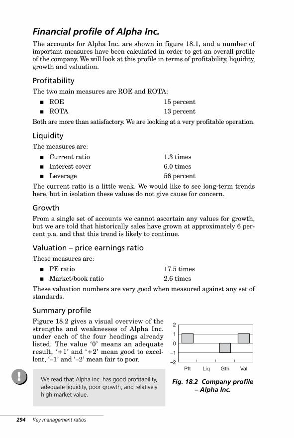
294 Key management ratios
Financial profile of Alpha Inc.The accounts for Alpha Inc. are shown in figure 18.1, and a number ofimportant measures have been calculated in order to get an overall profileof the company. We will look at this profile in terms of profitability, liquidity,growth and valuation.
ProfitabilityThe two main measures are ROE and ROTA:
■ ROE 15 percent■ ROTA 13 percent
Both are more than satisfactory. We are looking at a very profitable operation.
Liquidity The measures are:
■ Current ratio 1.3 times■ Interest cover 6.0 times■ Leverage 56 percent
The current ratio is a little weak. We would like to see long-term trendshere, but in isolation these values do not give cause for concern.
GrowthFrom a single set of accounts we cannot ascertain any values for growth,but we are told that historically sales have grown at approximately 6 per-cent p.a. and that this trend is likely to continue.
Valuation – price earnings ratioThese measures are:
■ PE ratio 17.5 times■ Market/book ratio 2.6 times
These valuation numbers are very good when measured against any set ofstandards.
Summary profileFigure 18.2 gives a visual overview of thestrengths and weaknesses of Alpha Inc.under each of the four headings alreadylisted. The value ‘0’ means an adequateresult, ‘+1’ and ‘+2’ mean good to excel-lent, ‘–1’ and ‘–2’ mean fair to poor.
We read that Alpha Inc. has good profitability,adequate liquidity, poor growth, and relativelyhigh market value.
!
2
1
0
–1
–2Pft Liq Gth Val
Fig. 18.2 Company profile– Alpha Inc.
WKMR_CH18.QXD 11/24/05 12:49 PM Page 294
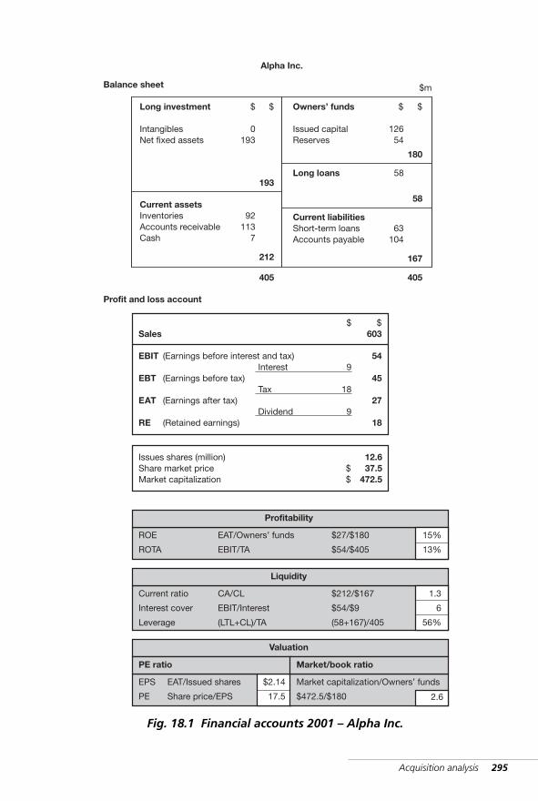
Acquisition analysis 295
Long investment
IntangiblesNet fixed assets
Current assetsInventoriesAccounts receivableCash
Owners’ funds
Issued capitalReserves
Long loans
Current liabilitiesShort-term loansAccounts payable
12654
$
180
$
58
63104
167
405
0193
$
193
$
92113
7
212
405
Balance sheet
Profit and loss account
$m
Alpha Inc.
Sales 603$
EBIT (Earnings before interest and tax)
EBT (Earnings before tax)
EAT (Earnings after tax)
RE (Retained earnings)
Interest
Tax
Dividend
9
18
9
54
45
27
18
$
58
Issues shares (million)Share market priceMarket capitalization
12.637.5
472.5$$
ROE
ROTA
EAT/Owners’ funds
EBIT/TA
$27/$180
$54/$405
Profitability
15%
13%
Current ratio
Interest cover
Leverage
CA/CL
EBIT/Interest
(LTL+CL)/TA
$212/$167
$54/$9
(58+167)/405
Liquidity
1.3
6
56%
Valuation
EPS
PE
EAT/Issued shares
Share price/EPS
$2.14
17.5
PE ratio
Market capitalization/Owners’ funds
$472.5/$180 2.6
Market/book ratio
Fig. 18.1 Financial accounts 2001 – Alpha Inc.
WKMR_CH18.QXD 11/24/05 12:49 PM Page 295
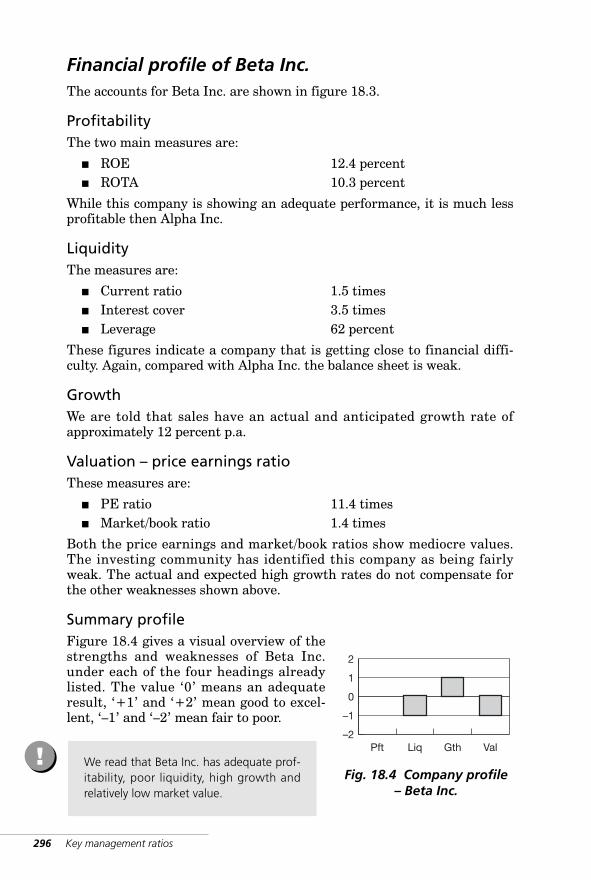
296 Key management ratios
Financial profile of Beta Inc.The accounts for Beta Inc. are shown in figure 18.3.
ProfitabilityThe two main measures are:
■ ROE 12.4 percent■ ROTA 10.3 percent
While this company is showing an adequate performance, it is much lessprofitable then Alpha Inc.
LiquidityThe measures are:
■ Current ratio 1.5 times■ Interest cover 3.5 times■ Leverage 62 percent
These figures indicate a company that is getting close to financial diffi-culty. Again, compared with Alpha Inc. the balance sheet is weak.
GrowthWe are told that sales have an actual and anticipated growth rate ofapproximately 12 percent p.a.
Valuation – price earnings ratioThese measures are:
■ PE ratio 11.4 times■ Market/book ratio 1.4 times
Both the price earnings and market/book ratios show mediocre values.The investing community has identified this company as being fairlyweak. The actual and expected high growth rates do not compensate forthe other weaknesses shown above.
Summary profileFigure 18.4 gives a visual overview of thestrengths and weaknesses of Beta Inc.under each of the four headings alreadylisted. The value ‘0’ means an adequateresult, ‘+1’ and ‘+2’ mean good to excel-lent, ‘–1’ and ‘–2’ mean fair to poor.
We read that Beta Inc. has adequate prof-itability, poor liquidity, high growth andrelatively low market value.
!
2
1
0
–1
–2Pft Liq Gth Val
Fig. 18.4 Company profile– Beta Inc.
WKMR_CH18.QXD 11/24/05 12:49 PM Page 296
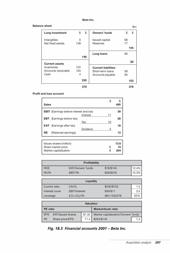
Acquisition analysis 297
Long investment
IntangiblesNet fixed assets
Current assetsInventoriesAccounts receivableCash
Owners’ funds
Issued capitalReserves
Long loans
Current liabilitiesShort-term loansAccounts payable
6877
$
145
$
80
5895
153
378
0148
$
148
$
122104
4
230
378
Balance sheet
Profit and loss account
$m
Beta Inc.
Sales 495$
EBIT (Earnings before interest and tax)
EBT (Earnings before tax)
EAT (Earnings after tax)
RE (Retained earnings)
Interest
Tax
Dividend
11
10
5
39
28
18
13
$
80
Issues shares (million)Share market priceMarket capitalization
13.615
204$$
ROE
ROTA
EAT/Owners’ funds
EBIT/TA
$18/$145
$39/$378
Profitability
12.4%
10.3%
Current ratio
Interest cover
Leverage
CA/CL
EBIT/Interest
(LTL+CL)/TA
$230/$153
$39/$11
(80+153)/378
Liquidity
1.5
3.5
62%
Valuation
EPS
PE
EAT/Issued shares
Share price/EPS
$1.32
11.4
PE ratio
Market capitalization/Owners’ funds
$204/$145 1.4
Market/book ratio
Fig. 18.3 Financial accounts 2001 – Beta Inc.
WKMR_CH18.QXD 11/24/05 12:49 PM Page 297
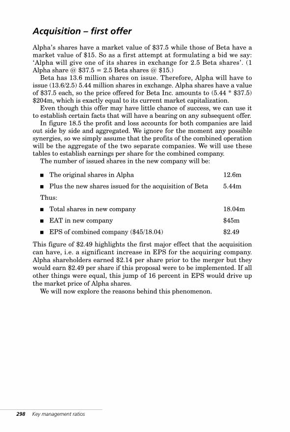
298 Key management ratios
Acquisition – first offer
Alpha’s shares have a market value of $37.5 while those of Beta have amarket value of $15. So as a first attempt at formulating a bid we say:‘Alpha will give one of its shares in exchange for 2.5 Beta shares’. (1Alpha share @ $37.5 = 2.5 Beta shares @ $15.)
Beta has 13.6 million shares on issue. Therefore, Alpha will have toissue (13.6/2.5) 5.44 million shares in exchange. Alpha shares have a valueof $37.5 each, so the price offered for Beta Inc. amounts to (5.44 * $37.5)$204m, which is exactly equal to its current market capitalization.
Even though this offer may have little chance of success, we can use itto establish certain facts that will have a bearing on any subsequent offer.
In figure 18.5 the profit and loss accounts for both companies are laidout side by side and aggregated. We ignore for the moment any possiblesynergies, so we simply assume that the profits of the combined operationwill be the aggregate of the two separate companies. We will use thesetables to establish earnings per share for the combined company.
The number of issued shares in the new company will be:
■ The original shares in Alpha 12.6m
■ Plus the new shares issued for the acquisition of Beta 5.44m
Thus:
■ Total shares in new company 18.04m
■ EAT in new company $45m
■ EPS of combined company ($45/18.04) $2.49
This figure of $2.49 highlights the first major effect that the acquisitioncan have, i.e. a significant increase in EPS for the acquiring company.Alpha shareholders earned $2.14 per share prior to the merger but theywould earn $2.49 per share if this proposal were to be implemented. If allother things were equal, this jump of 16 percent in EPS would drive upthe market price of Alpha shares.
We will now explore the reasons behind this phenomenon.
WKMR_CH18.QXD 11/24/05 12:49 PM Page 298
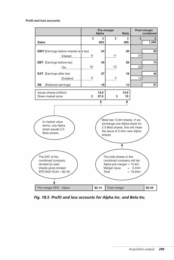
Acquisition analysis 299
Profit and loss accounts
Sales 603$
Interest
Tax
Dividend
9
18
9
54
45
27
18
$
Issues shares (million)Share market price
12.637.5$
11
10
5
$495
$
39
28
18
13
Pre-merger Post-mergercombinedBetaAlpha
20
28
14
$1,098
$
93
73
45
31
EBIT (Earnings before interest and tax)
EBT (Earnings before tax)
EAT (Earnings after tax)
RE (Retained earnings)
13.615$
Beta has 13.6m shares. If weexchange one Alpha share for2.5 Beta shares, this will meanthe issue of 5.44m new Alphashares.
The total shares in thecombined company will be:Alpha pre-merger = 12.6mMerger issue = 15.44mTotal = 18.04m
In market valueterms, one Alphashare equals 2.5Beta shares.
The EAT of thecombined companydivided by totalshares gives revisedEPS $45/18.04 = $2.49
Pre-merger EPS – Alpha $2.14 Post-merger $2.49
Fig. 18.5 Profit and loss accounts for Alpha Inc. and Beta Inc.
WKMR_CH18.QXD 11/24/05 12:49 PM Page 299
300 Key management ratios
Acquisition impact on EPS
It is the relative price to earnings ratios of the two shares that are the keyto understanding the increase in EPS of Alpha Inc.
The reasons are easy to explain. Prior to the acquisition, Alpha Inc. hadEAT of $27m. Post-acquisition, these profits have risen to $45m, i.e. anincrease of 66 percent. However, the increase in the number of shares hasonly been 5.44 million on the 12.6 million original issued shares in AlphaInc., i.e. an increase of 43 percent.
Thus a company on a high PE has a great advantage in the acquisitionprocess.
But we must also consider what has been the impact on Beta Inc. Theseshareholders have exchanged 2.5 old Beta shares for one new Alpha share.
We see in figure 18.3 that prior to the acquisition each Beta share com-manded an EPS of $1.33. Accordingly for 2.5 shares they should expect toreceive $3.3 (2.5 * $1.32) from each new Alpha share. In fact they receiveonly $2.49. This number translates back to $0.99 for each share that theyhave surrendered, which represents a loss of 24 percent.
Therefore, in terms of the important measure of EPS, Alpha sharehold-ers have benefited to the extent of 16 percent, while Beta shareholdershave suffered a loss of 24 percent.
There are other variables of interest to both sets of shareholders thatare also affected by the merger, and these will now be explored.
When company A acquires company B by means of a straight exchange of sharesand when that exchange is made exactly at the market prices of the two shares,then if company A has a higher price to earnings ratio than company B, companyA gains an automatic increase in EPS.
!
We see in figures 18.1 and 18.3 that, whereas the Alpha Inc. PE was 17.5 times,the corresponding number for Beta Inc. was 11.4 times, and it this difference inPE values that has enabled Alpha Inc. to acquire 66 percent extra profit for anincrease of only 43 percent in the number of shares (see figure 18.6).
!
WKMR_CH18.QXD 11/24/05 12:49 PM Page 300
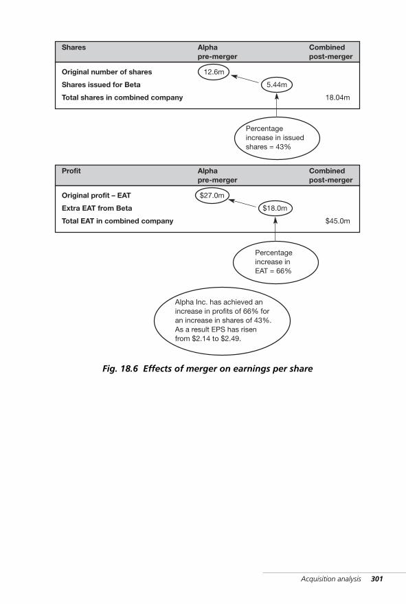
Acquisition analysis 301
Original number of shares
Shares issued for Beta
Total shares in combined company
Shares Alphapre-merger
Combinedpost-merger
18.04m
5.44m
12.6m
Original profit – EAT
Extra EAT from Beta
Total EAT in combined company
Profit Alphapre-merger
Combinedpost-merger
$45.0m
$18.0m
$27.0m
Percentageincrease in issuedshares = 43%
Percentageincrease inEAT = 66%
Alpha Inc. has achieved anincrease in profits of 66% foran increase in shares of 43%.As a result EPS has risenfrom $2.14 to $2.49.
Fig. 18.6 Effects of merger on earnings per share
WKMR_CH18.QXD 11/24/05 12:49 PM Page 301
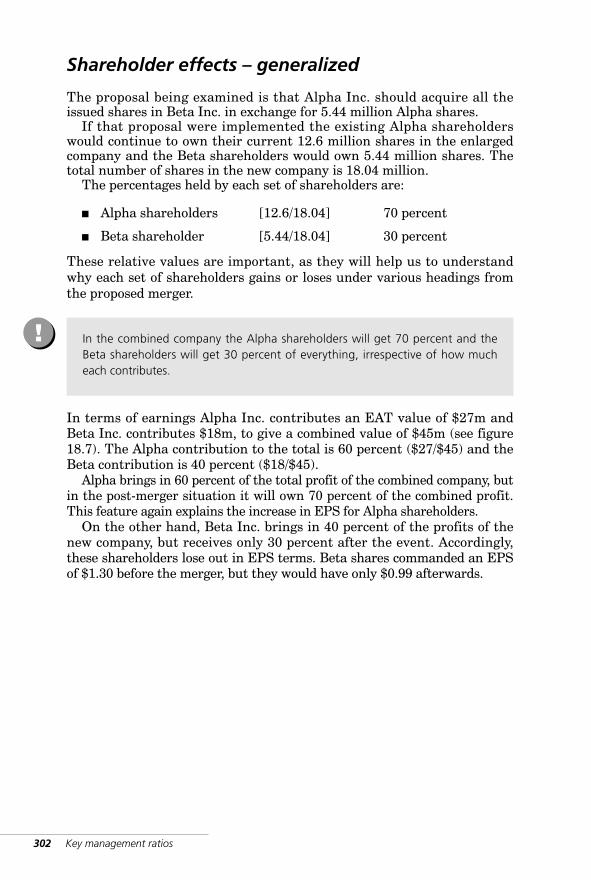
302 Key management ratios
Shareholder effects – generalized
The proposal being examined is that Alpha Inc. should acquire all theissued shares in Beta Inc. in exchange for 5.44 million Alpha shares.
If that proposal were implemented the existing Alpha shareholderswould continue to own their current 12.6 million shares in the enlargedcompany and the Beta shareholders would own 5.44 million shares. Thetotal number of shares in the new company is 18.04 million.
The percentages held by each set of shareholders are:
■ Alpha shareholders [12.6/18.04] 70 percent
■ Beta shareholder [5.44/18.04] 30 percent
These relative values are important, as they will help us to understandwhy each set of shareholders gains or loses under various headings fromthe proposed merger.
In terms of earnings Alpha Inc. contributes an EAT value of $27m andBeta Inc. contributes $18m, to give a combined value of $45m (see figure18.7). The Alpha contribution to the total is 60 percent ($27/$45) and theBeta contribution is 40 percent ($18/$45).
Alpha brings in 60 percent of the total profit of the combined company, butin the post-merger situation it will own 70 percent of the combined profit.This feature again explains the increase in EPS for Alpha shareholders.
On the other hand, Beta Inc. brings in 40 percent of the profits of thenew company, but receives only 30 percent after the event. Accordingly,these shareholders lose out in EPS terms. Beta shares commanded an EPSof $1.30 before the merger, but they would have only $0.99 afterwards.
In the combined company the Alpha shareholders will get 70 percent and theBeta shareholders will get 30 percent of everything, irrespective of how mucheach contributes.
!
WKMR_CH18.QXD 11/24/05 12:49 PM Page 302
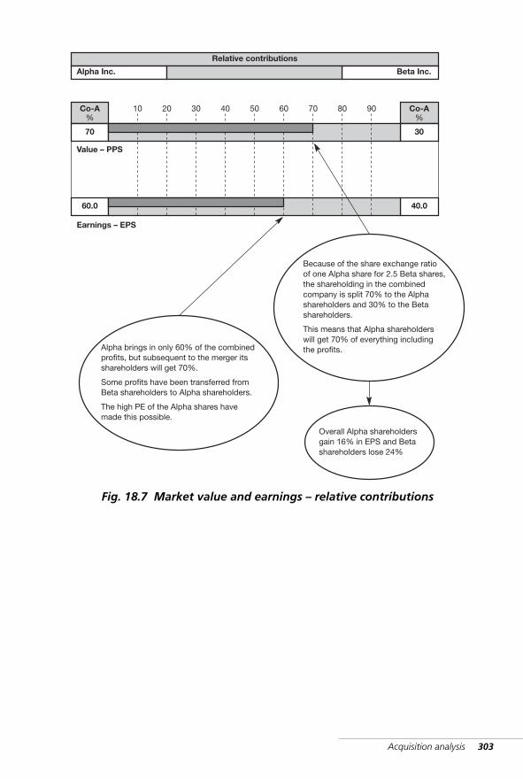
Acquisition analysis 303
Alpha Inc. Beta Inc.
Relative contributions
70 30
Co-A%
Co-A%
10 20 30 40 50 60 70 80 90
Value – PPS
Earnings – EPS
60.0 40.0
Because of the share exchange ratioof one Alpha share for 2.5 Beta shares,the shareholding in the combinedcompany is split 70% to the Alphashareholders and 30% to the Betashareholders.
This means that Alpha shareholderswill get 70% of everything includingthe profits.
Overall Alpha shareholdersgain 16% in EPS and Betashareholders lose 24%
Alpha brings in only 60% of the combinedprofits, but subsequent to the merger itsshareholders will get 70%.
Some profits have been transferred fromBeta shareholders to Alpha shareholders.
The high PE of the Alpha shares havemade this possible.
Fig. 18.7 Market value and earnings – relative contributions
WKMR_CH18.QXD 11/24/05 12:49 PM Page 303
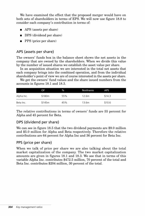
304 Key management ratios
We have examined the effect that the proposed merger would have onboth sets of shareholders in terms of EPS. We will now use figure 18.8 toconsider each company’s contribution in terms of:
■ APS (assets per share)
■ DPS (dividend per share)
■ PPS (price per share)
APS (assets per share)
The owners’ funds box in the balance sheet shows the net assets in thecompany that are owned by the shareholders. When we divide this valueby the number of issued shares we establish the asset value per share.
In an acquisition situation we are interested in the total net assets thateach company brings into the combined operation, and from the individualshareholder’s point of view we are of course interested in the assets per share.
We get the owners’ fund values and the share issued numbers from theaccounts in figures 18.1 and 18.3.
OF % No/shares APS
Alpha Inc. $180m 55% 12.6m $14.3
Beta Inc. $145m 45% 13.6m $10.6
The relative contributions in terms of owners’ funds are 55 percent forAlpha and 45 percent for Beta.
DPS (dividend per share)
We can see in figure 18.5 that the two dividend payments are $9.0 millionand $5.0 million for Alpha and Beta respectively. Therefore the relativecontributions are 64 percent for Alpha Inc and 36 percent for Beta Inc.
PPS (price per share)
When we talk of price per share we are also talking about the totalmarket capitalization of the company. The two market capitalizationamounts are given in figures 18.1 and 18.3. We see that in terms of thisvariable Alpha Inc. contributes $472.5 million, 70 percent of the total andBeta Inc. contributes $204 million, 30 percent of the total.
WKMR_CH18.QXD 11/24/05 12:49 PM Page 304
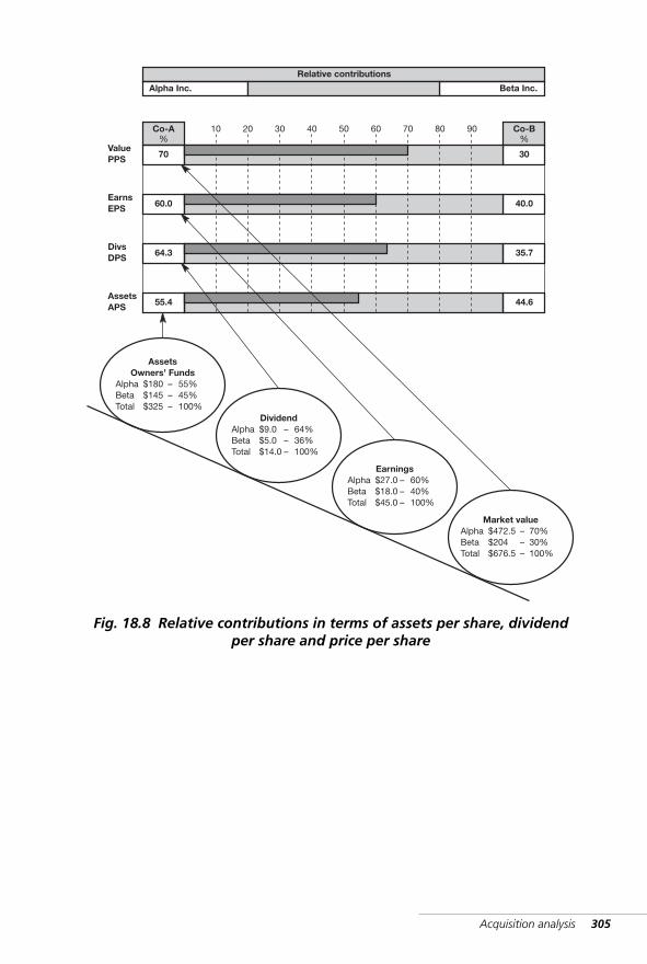
Acquisition analysis 305
Alpha Inc. Beta Inc.
Relative contributions
70 30
Co-A%
Co-B%
10 20 30 40 50 60 70 80 90
ValuePPS
EarnsEPS 60.0 40.0
AssetsOwners’ Funds
Alpha $180 – 55%Beta $145 – 45%Total $325 – 100%
DivsDPS 64.3 35.7
AssetsAPS 55.4 44.6
DividendAlpha $9.0 – 64%Beta $5.0 – 36%Total $14.0 – 100%
EarningsAlpha $27.0 – 60%Beta $18.0 – 40%Total $45.0 – 100%
Market valueAlpha $472.5 – 70%Beta $204 – 30%Total $676.5 – 100%
Fig. 18.8 Relative contributions in terms of assets per share, dividendper share and price per share
WKMR_CH18.QXD 11/24/05 12:49 PM Page 305
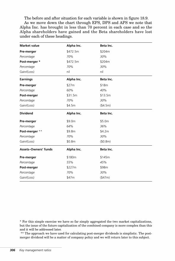
306 Key management ratios
* For this simple exercise we have so far simply aggregated the two market capitalizations,but the issue of the future capitalization of the combined company is more complex than thisand it will be addressed later.** The approach we have used for calculating post-merger dividends is simplistic. The post-
merger dividend will be a matter of company policy and we will return later to this subject.
The before and after situation for each variable is shown in figure 18.9.As we move down the chart through EPS, DPS and APS we note that
Alpha Inc. has brought in less than 70 percent in each case and so theAlpha shareholders have gained and the Beta shareholders have lostunder each of these headings.
Market value Alpha Inc. Beta Inc.
Pre-merger $472.5m $204m
Percentage 70% 30%
Post-merger * $472.5m $204m
Percentage 70% 30%
Gain/(Loss) nil nil
Earnings Alpha Inc. Beta Inc.
Pre-merger $27m $18m
Percentage 60% 40%
Post-merger $31.5m $13.5m
Percentage 70% 30%
Gain/(Loss) $4.5m ($4.5m)
Dividend Alpha Inc. Beta Inc.
Pre-merger $9.0m $5.0m
Percentage 64% 36%
Post-merger ** $9.8m $4.2m
Percentage 70% 30%
Gain/(Loss) $0.8m ($0.8m)
Assets–Owners’ funds Alpha Inc. Beta Inc.
Pre-merger $180m $145m
Percentage 55% 45%
Post-merger $227m $98m
Percentage 70% 30%
Gain/(Loss) $47m ($47m)
WKMR_CH18.QXD 11/24/05 12:49 PM Page 306
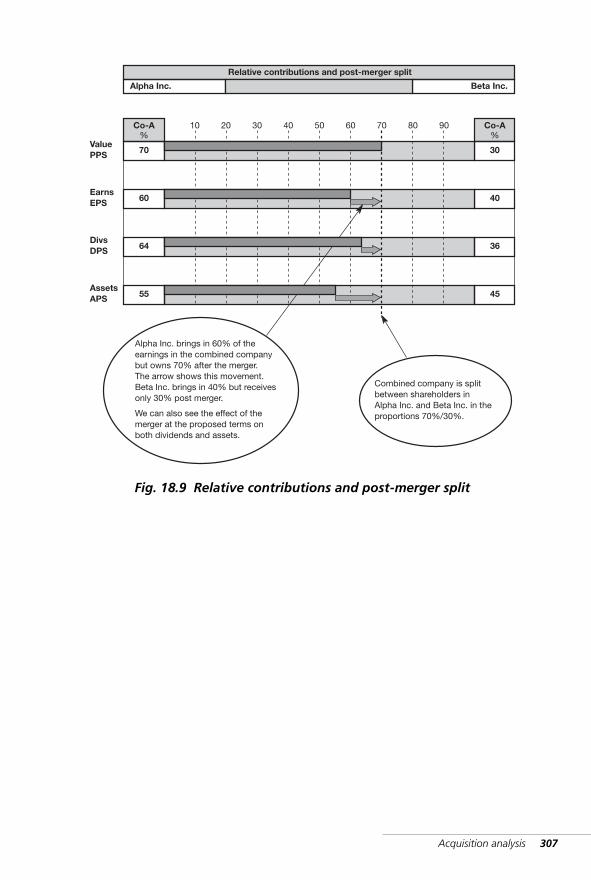
Acquisition analysis 307
Alpha Inc. Beta Inc.
Relative contributions and post-merger split
70 30
Co-A%
Co-A%
10 20 30 40 50 60 70 80 90
ValuePPS
EarnsEPS 60 40
DivsDPS 64 36
AssetsAPS 55 45
Alpha Inc. brings in 60% of theearnings in the combined companybut owns 70% after the merger.The arrow shows this movement.Beta Inc. brings in 40% but receivesonly 30% post merger.
We can also see the effect of themerger at the proposed terms onboth dividends and assets.
Combined company is splitbetween shareholders inAlpha Inc. and Beta Inc. in theproportions 70%/30%.
Fig. 18.9 Relative contributions and post-merger split
WKMR_CH18.QXD 11/24/05 12:49 PM Page 307
308 Key management ratios
Summary of effects on shareholders
In figure 18.10 we show the results for the two sets of shareholders underthe four separate headings.
Apart from the prices per share which remain unchanged for both par-ties, all the financial gains from the acquisition accrue to the Alphashareholders and all the losses to the Beta shareholders.
The sole reason for this outcome is that Alpha Inc. has a much higherPE (price earnings ratio) than Beta Inc. and the shares were exchangedon the basis of their relative market prices.
So a high PE is a very powerful weapon in a takeover contest. In fact itis pretty well impossible for a low PE company to acquire another usingshares for all or part of the consideration.
But to return to our Alpha/Beta example, while all the gains go to theAlpha shareholders it is not likely that the Beta shareholders will buy intothe proposal. First because there is a 20 per cent loss in dividend. Thelosses in the areas of earnings and assets (EPS and APS) may be of moreinterest to management, but to the investor the total market value of theshares and the annual dividend paid are the crucial issues.
So if Alpha Inc. really desires to acquire Beta Inc. an increased offerwill be necessary. This new offer could be a mixture of shares and cash, allcash, or simply a greater number of shares.
The possible combinations are endless, but overleaf we have puttogether an increased offer of 6.5 million shares and an increase in thedividend that appears to give Beta shareholders what they would require,i.e. increased market value and no loss of dividend. At the same time, itgives to Alpha Inc. a very desirable increase in earnings per share.
WKMR_CH18.QXD 11/24/05 12:49 PM Page 308
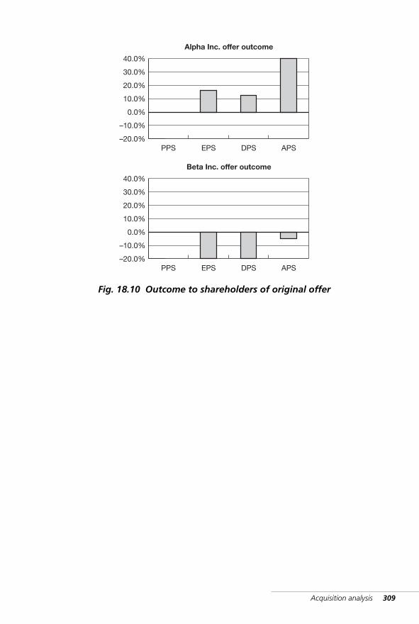
Acquisition analysis 309
40.0%
30.0%
20.0%
10.0%
–20.0%PPS EPS DPS APS
0.0%
–10.0%
Beta Inc. offer outcome
Fig. 18.10 Outcome to shareholders of original offer
40.0%
30.0%
20.0%
10.0%
–20.0%PPS EPS DPS APS
0.0%
–10.0%
Alpha Inc. offer outcome
WKMR_CH18.QXD 11/24/05 12:49 PM Page 309
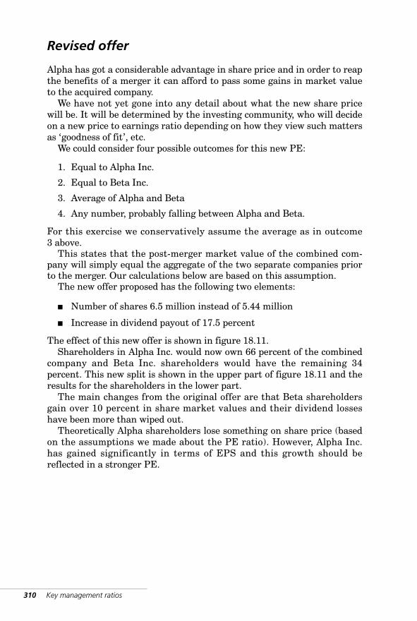
310 Key management ratios
Revised offer
Alpha has got a considerable advantage in share price and in order to reapthe benefits of a merger it can afford to pass some gains in market valueto the acquired company.
We have not yet gone into any detail about what the new share pricewill be. It will be determined by the investing community, who will decideon a new price to earnings ratio depending on how they view such mattersas ‘goodness of fit’, etc.
We could consider four possible outcomes for this new PE:
1. Equal to Alpha Inc.
2. Equal to Beta Inc.
3. Average of Alpha and Beta
4. Any number, probably falling between Alpha and Beta.
For this exercise we conservatively assume the average as in outcome3 above.
This states that the post-merger market value of the combined com-pany will simply equal the aggregate of the two separate companies priorto the merger. Our calculations below are based on this assumption.
The new offer proposed has the following two elements:
■ Number of shares 6.5 million instead of 5.44 million
■ Increase in dividend payout of 17.5 percent
The effect of this new offer is shown in figure 18.11.Shareholders in Alpha Inc. would now own 66 percent of the combined
company and Beta Inc. shareholders would have the remaining 34percent. This new split is shown in the upper part of figure 18.11 and theresults for the shareholders in the lower part.
The main changes from the original offer are that Beta shareholdersgain over 10 percent in share market values and their dividend losseshave been more than wiped out.
Theoretically Alpha shareholders lose something on share price (basedon the assumptions we made about the PE ratio). However, Alpha Inc.has gained significantly in terms of EPS and this growth should bereflected in a stronger PE.
WKMR_CH18.QXD 11/24/05 12:49 PM Page 310
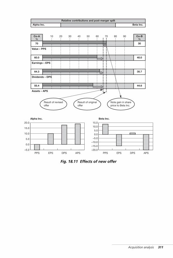
Acquisition analysis 311
Alpha Inc. Beta Inc.
Relative contributions and post-merger split
70 30
Co-A%
Co-B%
10 20 30 40 50 60 70 80 90
Value – PPS
Earnings – EPS
60.0 40.0
Dividends – DPS
64.3 35.7
Assets – APS
55.4 44.6
Result of revisedoffer
Result of originaloffer
Note gain in shareprice to Beta Inc.
20.0
15.0
10.0
5.0
–5.0PPS EPS DPS APS
0.0
Alpha Inc.
15.0
10.0
0.0
–5.0
–20.0PPS EPS DPS APS
–10.0
Beta Inc.
–15.0
5.0
Fig. 18.11 Effects of new offer
WKMR_CH18.QXD 11/24/05 12:49 PM Page 311
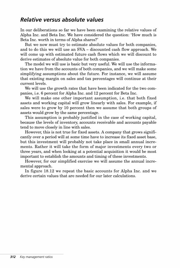
312 Key management ratios
Relative versus absolute values
In our deliberations so far we have been examining the relative values ofAlpha Inc. and Beta Inc. We have considered the question: ‘How much isBeta Inc. worth in terms of Alpha shares?’
But we now must try to estimate absolute values for both companies,and to do this we will use an SVA – discounted cash flow approach. Wewill come up with estimated future cash flows which we will discount toderive estimates of absolute value for both companies.
The model we will use is basic but very useful. We will use the informa-tion we have from the accounts of both companies, and we will make somesimplifying assumptions about the future. For instance, we will assumethat existing margin on sales and tax percentages will continue at theircurrent levels.
We will use the growth rates that have been indicated for the two com-panies, i.e. 6 percent for Alpha Inc. and 12 percent for Beta Inc.
We will make one other important assumption, i.e. that both fixedassets and working capital will grow linearly with sales. For example, ifsales were to grow by 10 percent then we assume that both groups ofassets would grow by the same percentage.
This assumption is probably justified in the case of working capital,because the levels of inventory, accounts receivable and accounts payabletend to move closely in line with sales.
However, this is not true for fixed assets. A company that grows signifi-cantly over a period will at some time have to increase its fixed asset base,but this investment will probably not take place in small annual incre-ments. Rather it will take the form of major investments every two orthree years, and when looking at a potential acquisition it would be mostimportant to establish the amounts and timing of these investments.
However, for our simplified exercise we will assume the annual incre-mental approach.
In figure 18.12 we repeat the basic accounts for Alpha Inc. and wederive certain values that are needed for our later calculations.
WKMR_CH18.QXD 11/24/05 12:49 PM Page 312
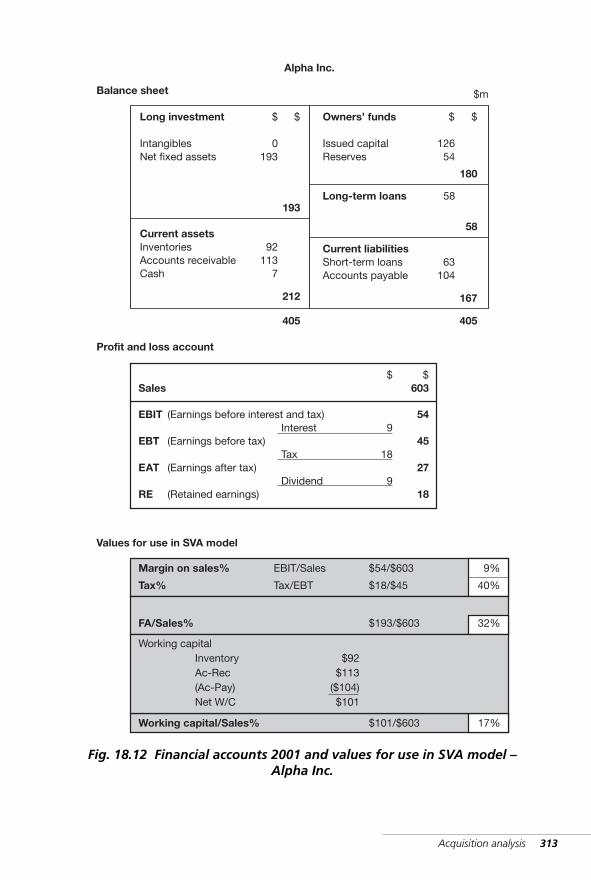
Acquisition analysis 313
Long investment
IntangiblesNet fixed assets
Current assetsInventoriesAccounts receivableCash
Owners’ funds
Issued capitalReserves
Long-term loans
Current liabilitiesShort-term loansAccounts payable
12654
$
180
$
58
63104
167
405
0193
$
193
$
92113
7
212
405
Balance sheet
Profit and loss account
$m
Alpha Inc.
Sales 603$
EBIT (Earnings before interest and tax)
EBT (Earnings before tax)
EAT (Earnings after tax)
RE (Retained earnings)
Interest
Tax
Dividend
9
18
9
54
45
27
18
$
58
Margin on sales%
Tax%
EBIT/Sales
Tax/EBT
$54/$603
$18/$45
9%
40%
Values for use in SVA model
FA/Sales% $193/$603 32%
Working capitalInventoryAc-Rec(Ac-Pay)Net W/C
$92$113
($104)$101
Working capital/Sales% $101/$603 17%
Fig. 18.12 Financial accounts 2001 and values for use in SVA model –Alpha Inc.
WKMR_CH18.QXD 11/24/05 12:49 PM Page 313
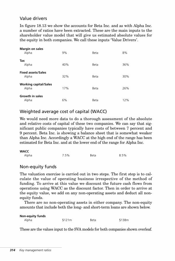
314 Key management ratios
Value drivers
In figure 18.13 we show the accounts for Beta Inc. and as with Alpha Inc.a number of ratios have been extracted. These are the main inputs to theshareholder value model that will give us estimated absolute values forthe equity in both companies. We call these inputs ‘Value Drivers’.
Margin on salesAlpha 9% Beta 8%
TaxAlpha 40% Beta 36%
Fixed assets/SalesAlpha 32% Beta 30%
Working capital/SalesAlpha 17% Beta 26%
Growth in salesAlpha 6% Beta 12%
Weighted average cost of capital (WACC)
We would need more data to do a thorough assessment of the absoluteand relative costs of capital of these two companies. We can say that sig-nificant public companies typically have costs of between 7 percent and9 percent. Beta Inc. is showing a balance sheet that is somewhat weakerthan Alpha Inc. Accordingly a WACC at the high end of the range has beenestimated for Beta Inc. and at the lower end of the range for Alpha Inc.
WACCAlpha 7.5% Beta 8.5%
Non-equity funds
The valuation exercise is carried out in two steps. The first step is to cal-culate the value of operating business irrespective of the method offunding. To arrive at this value we discount the future cash flows fromoperations using WACC as the discount factor. Then in order to arrive atthe equity value, we add on any non-operating assets and deduct all non-equity funds.
There are no non-operating assets in either company. The non-equityamounts that include both the long- and short-term loans are shown below.
Non-equity fundsAlpha $121m Beta $138m
These are the values input to the SVA models for both companies shown overleaf.
WKMR_CH18.QXD 11/24/05 12:49 PM Page 314
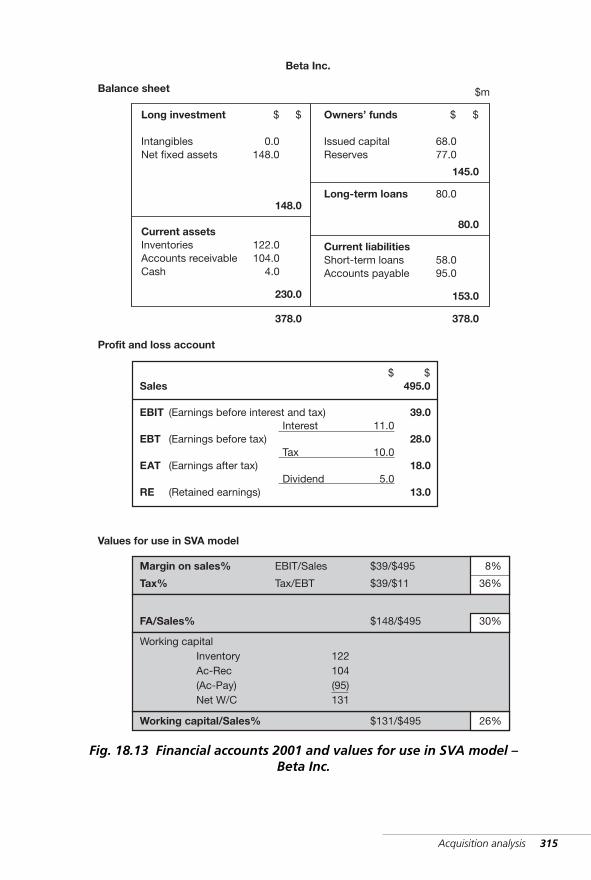
Acquisition analysis 315
Long investment
IntangiblesNet fixed assets
Current assetsInventoriesAccounts receivableCash
Owners’ funds
Issued capitalReserves
Long-term loans
Current liabilitiesShort-term loansAccounts payable
68.077.0
$
145.0
$
80.0
58.095.0
153.0
378.0
0.0148.0
$
148.0
$
122.0104.0
4.0
230.0
378.0
Balance sheet
Profit and loss account
$m
Beta Inc.
Sales 495.0$
EBIT (Earnings before interest and tax)
EBT (Earnings before tax)
EAT (Earnings after tax)
RE (Retained earnings)
Interest
Tax
Dividend
11.0
10.0
5.0
39.0
28.0
18.0
13.0
$
80.0
Margin on sales%
Tax%
EBIT/Sales
Tax/EBT
$39/$495
$39/$11
8%
36%
Values for use in SVA model
FA/Sales% $148/$495 30%
Working capitalInventoryAc-Rec(Ac-Pay)Net W/C
122104(95)131
Working capital/Sales% $131/$495 26%
Fig. 18.13 Financial accounts 2001 and values for use in SVA model –Beta Inc.
WKMR_CH18.QXD 11/24/05 12:49 PM Page 315
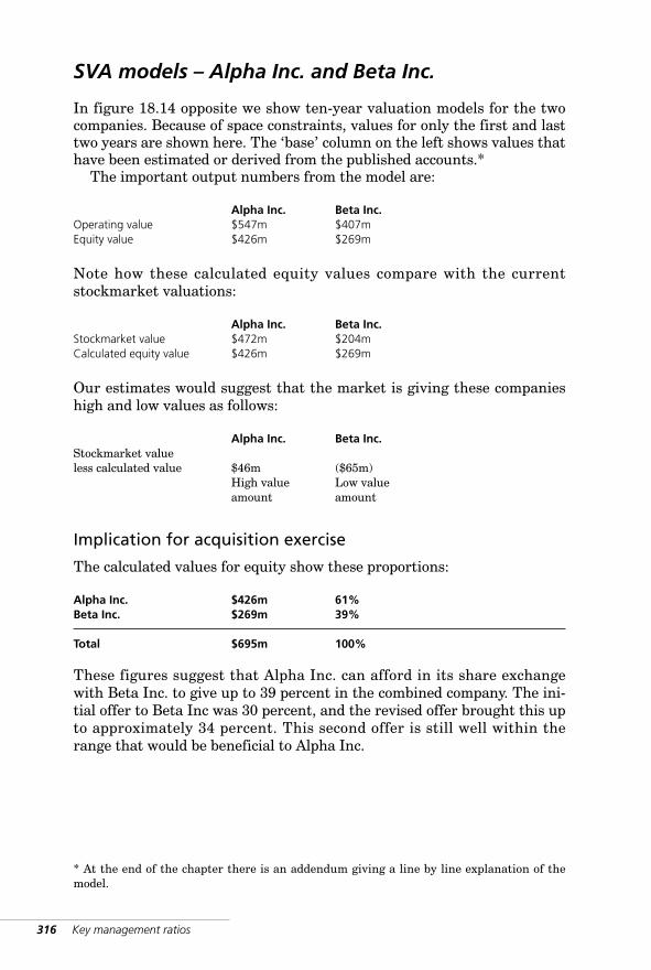
316 Key management ratios
SVA models – Alpha Inc. and Beta Inc.
In figure 18.14 opposite we show ten-year valuation models for the twocompanies. Because of space constraints, values for only the first and lasttwo years are shown here. The ‘base’ column on the left shows values thathave been estimated or derived from the published accounts.*
The important output numbers from the model are:
Alpha Inc. Beta Inc.Operating value $547m $407mEquity value $426m $269m
Note how these calculated equity values compare with the currentstockmarket valuations:
Alpha Inc. Beta Inc.Stockmarket value $472m $204mCalculated equity value $426m $269m
Our estimates would suggest that the market is giving these companieshigh and low values as follows:
Alpha Inc. Beta Inc.Stockmarket valueless calculated value $46m ($65m)
High value Low valueamount amount
Implication for acquisition exercise
The calculated values for equity show these proportions:
Alpha Inc. $426m 61%Beta Inc. $269m 39%
Total $695m 100%
These figures suggest that Alpha Inc. can afford in its share exchangewith Beta Inc. to give up to 39 percent in the combined company. The ini-tial offer to Beta Inc was 30 percent, and the revised offer brought this upto approximately 34 percent. This second offer is still well within therange that would be beneficial to Alpha Inc.
* At the end of the chapter there is an addendum giving a line by line explanation of themodel.
WKMR_CH18.QXD 11/24/05 12:49 PM Page 316
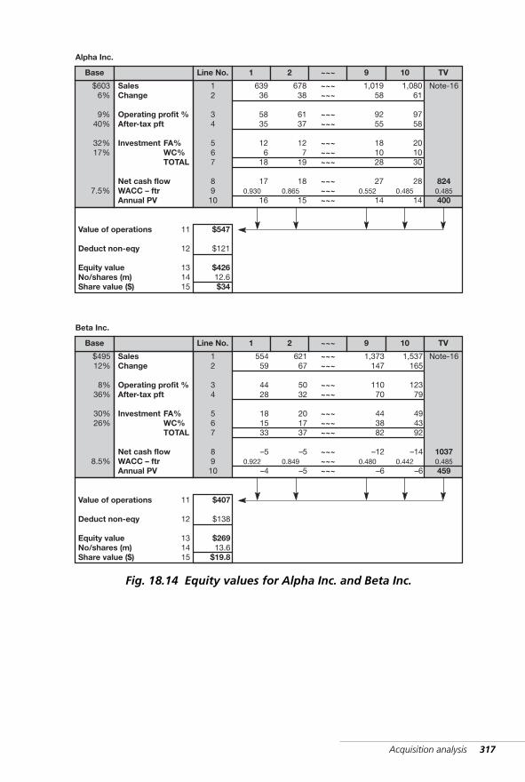
Acquisition analysis 317
SalesChange
Operating profit %After-tax pft
Investment FA%WC%TOTAL
Net cash flowWACC – ftrAnnual PV
$6036%
9%40%
32%17%
7.5%
Base
Alpha Inc.
12
34
567
8910
Line No. 1 2 ~~~ 9 10 TV
Note-16
8240.485400
63936
5835
126
18
17
16
67838
6137
127
19
18
15
~~~~~~
~~~~~~
~~~~~~~~~
~~~~~~~~~
1,01958
9255
181028
27
14
1,08061
9758
201030
28
140.4850.5520.8650.930
Value of operations
Deduct non-eqy
Equity valueNo/shares (m)Share value ($)
11
12
131415
$547
$121
$42612.6$34
SalesChange
Operating profit %After-tax pft
Investment FA%WC%TOTAL
Net cash flowWACC – ftrAnnual PV
$49512%
8%36%
30%26%
8.5%
Base
Beta Inc.
12
34
567
8910
Line No. 1 2 ~~~ 9 10 TV
Note-16
10370.485459
55459
4428
181533
–5
–4
62167
5032
201737
–5
–5
~~~~~~
~~~~~~
~~~~~~~~~
~~~~~~~~~
1,373147
11070
443882
–12
–6
1,537165
12379
494392
–14
–60.4420.4800.8490.922
Value of operations
Deduct non-eqy
Equity valueNo/shares (m)Share value ($)
11
12
131415
$407
$138
$26913.6
$19.8
Fig. 18.14 Equity values for Alpha Inc. and Beta Inc.
WKMR_CH18.QXD 11/24/05 12:49 PM Page 317
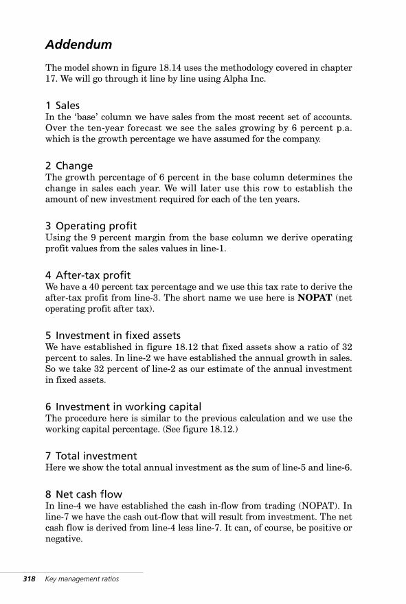
318 Key management ratios
Addendum
The model shown in figure 18.14 uses the methodology covered in chapter17. We will go through it line by line using Alpha Inc.
1 SalesIn the ‘base’ column we have sales from the most recent set of accounts.Over the ten-year forecast we see the sales growing by 6 percent p.a.which is the growth percentage we have assumed for the company.
2 ChangeThe growth percentage of 6 percent in the base column determines thechange in sales each year. We will later use this row to establish theamount of new investment required for each of the ten years.
3 Operating profitUsing the 9 percent margin from the base column we derive operatingprofit values from the sales values in line-1.
4 After-tax profitWe have a 40 percent tax percentage and we use this tax rate to derive theafter-tax profit from line-3. The short name we use here is NOPAT (netoperating profit after tax).
5 Investment in fixed assetsWe have established in figure 18.12 that fixed assets show a ratio of 32percent to sales. In line-2 we have established the annual growth in sales.So we take 32 percent of line-2 as our estimate of the annual investmentin fixed assets.
6 Investment in working capitalThe procedure here is similar to the previous calculation and we use theworking capital percentage. (See figure 18.12.)
7 Total investmentHere we show the total annual investment as the sum of line-5 and line-6.
8 Net cash flowIn line-4 we have established the cash in-flow from trading (NOPAT). Inline-7 we have the cash out-flow that will result from investment. The netcash flow is derived from line-4 less line-7. It can, of course, be positive ornegative.
WKMR_CH18.QXD 11/24/05 12:49 PM Page 318
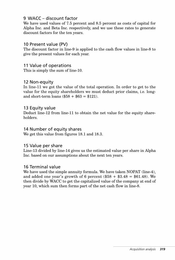
9 WACC – discount factorWe have used values of 7.5 percent and 8.5 percent as costs of capital forAlpha Inc. and Beta Inc. respectively, and we use these rates to generatediscount factors for the ten years.
10 Present value (PV)The discount factor in line-9 is applied to the cash flow values in line-8 togive the present values for each year.
11 Value of operationsThis is simply the sum of line-10.
12 Non-equityIn line-11 we got the value of the total operation. In order to get to thevalue for the equity shareholders we must deduct prior claims, i.e. long-and short-term loans ($58 + $63 = $121).
13 Equity valueDeduct line-12 from line-11 to obtain the net value for the equity share-holders.
14 Number of equity sharesWe get this value from figures 18.1 and 18.3.
15 Value per shareLine-13 divided by line-14 gives us the estimated value per share in AlphaInc. based on our assumptions about the next ten years.
16 Terminal valueWe have used the simple annuity formula. We have taken NOPAT (line-4),and added one year’s growth of 6 percent ($58 + $3.48 = $61.48). Wethen divide by WACC to get the capitalized value of the company at end ofyear 10, which sum then forms part of the net cash flow in line-8.
Acquisition analysis 319
WKMR_CH18.QXD 11/24/05 12:49 PM Page 319

WKMR_CH18.QXD 11/24/05 12:49 PM Page 320
19 Integrity ofaccountingstatements*Introduction · Where we focus
attention · Operating revenue
enhancement · Methods of revenue
enhancement – fictitious sales ·Revenue enhancement – clues for
detection · Operating cost · The
balance sheet · The cash flow
statement
To mischief trained, e’en from his mother’s womb,Grown old in fraud, tho’ yet in manhood’s bloom.
Adopting arts, by which gay villains rise,And reach the heights, which honest men despise;LORD LOUGHBOROUGH (1761)
* Two recomended publications that deal exclusively with thissubject are: The Financial Numbers Game, Mulford andComiskey, John Wiley; and, Financial Shenanigans, HowardSchilit, McGraw Hill.
WKMR_CH19.QXD 11/24/05 12:49 PM Page 321

WKMR_CH19.QXD 11/24/05 12:49 PM Page 322
Integrity of accounting statements 323
Introduction
The material in this book so far has been concerned with how we can usevalues in the published accounts of a company to give us informationabout its overall performance.
But how certain are we that the numbers shown in the accounts do infact reflect reality and give us a true picture of the state of affairs in theorganization concerned? The answer is that in the vast majority of caseswe can be certain because of the great scrutiny that these numbers aresubject to from the investment community, the banking fraternity and thevarious regulatory bodies that govern business affairs, for example, theSEC (Securities and Exchange Commission), the stock exchange, theaccounting institutes, etc. These bodies have derived very detailed regula-tions governing the presentation of annual accounts and these regulationsare constantly being updated to reflect changing circumstances.
Nevertheless because of the diversity of different business situationsthese regulations cannot be too prescriptive. A certain leeway is still per-mitted to managers and where companies do not wish to show the truestate of affairs, where for various reasons their intent is to present a pic-ture that is more optimistic than justified by the true operatingperformance, there is still scope for some creative accounting.
Accordingly accounts may be produced where some of the numbershave been manipulated. The purpose of this chapter is to show the morelikely areas where such manipulations can occur, and to indicate howsome of these may be detected.
Occasionally a company will wish to present accounts that understateperformance. This is a much less frequent occurrence and this chapterwill concentrate on overstated accounts.
As the subject is constantly evolving, there are still areas in reportedaccounts where even the most diligent investigator can, at least for ashort time, be deceived.
☛
WKMR_CH19.QXD 11/24/05 12:49 PM Page 323
324 Key management ratios
Where we focus attention
We know what the factors are which determine a company’s overall ratingin the marketplace, i.e:
■ profitability ■ liquidity ■ growth.
It is useful to remember at this stage that if a number anywhere in theaccounts is altered or exaggerated then there has to be a balancingchange somewhere else in the accounts. For instance if we show an exag-gerated profit in the income statement the amount of the exaggerationwill appear either as an enhanced asset or reduced liability in the balancesheet. We can therefore always look for a possible manipulation in twoseparate sections of the accounts.
The ‘notes to accounts’ that always accompany the published state-ments are a very fertile source of information even if they are oftenwritten in tedious and obscure language. Nevertheless they must be readmost diligently because each phrase is carefully constructed and designedto portray the information that regulations demand and often not onewhit more than that information.
Of particular interest should be the note on ‘accounting policies’. This iswhere many of the principles governing the accounts in question arespecifically identified. A change in one of the policies, for example, depre-ciation policy, could be a strong warning signal and pointer towards theneed for further investigation.
The next most fertile area of investigation lies with the various ratiosthat have been detailed in the early chapters in this publication.
It is in one or more of these areas that numbers are most likely to be changed inorder to give a false picture of the company. So we look to those areas in thefinancial statements that give information on these three factors, i.e. for prof-itability we examine the income statement, for a liquidity assessment we look tothe balance sheet and cash flow statement and for an evaluation of growth welook to the revenue stream.
!
☛
✓
WKMR_CH19.QXD 11/24/05 12:49 PM Page 324
Integrity of accounting statements 325
Operating revenue enhancement
Operating revenue is revenue that derives from the core business of acorporation. It is distinguished from non-operating revenue, for example,the once-off sale of a fixed asset that, because of its non-recurring nature,would not be considered to be an indicator of current or future businessperformance. We use the same distinction in relation to operating andnon-operating income and operating and non-operating cost.
Revenue recognition
Therefore it is important to consider when revenue can be recognized inthe books of account. The rules are very precise.
Revenue is earned when a product or service is fully delivered* byarrangement to a customer at an agreed price and the customerunconditionally accepts the corresponding financial liability and willprobably be able to meet this liability.
The most powerful way to affect disclosed profitability is to alter thefigure for operating revenue. There are three ways in which this can beachieved, as shown overleaf.
We can distinguish three methods by which operating revenue can beartificially inflated:
■ By incorrectly moving revenue from one time period into another.This generally involves bringing revenue which should properly beshown in a future time period back to the current period –premature revenue.
■ By recording sales which do not exist – fictitious revenue.■ By including one-time gains as normal operating revenue –
wrongly classified revenue.
✓
Operating revenue and its rate of growth are perhaps the two most importantkey variables to be considered in evaluating overall corporate financial perform-ance. It is in the area of operating revenue taken from the profit and loss accountand often referred to as the ‘top line’, that approximately two-thirds of allattempts to enhance a company’s performance are made.
!
WKMR_CH19.QXD 11/24/05 12:49 PM Page 325
326 Key management ratios
Premature revenue
We can incorrectly take revenue from a future period back into the pres-ent time period in the following ways.
Method 1 – backdating
The simplest way to move revenue into a current period from the succeed-ing one is simply to alter the cut-off date or backdate invoices and/ordelivery notes. This may even involve changing the date in the computer.This, of course, has a very-short-term effect and if enhancement of rev-enue is required over a number of time periods the effect is cumulativeand likely to become visible within a short time.
Method 2 – stuffed revenue
Sometimes a company will generate increased revenue for a period byoffering customers special inducements, for example, major discounts orbonuses, to take product before they require it and in excess of any salesforecasts. This is called ‘stuffing the channel’. These sales appear to begenuine but they are not appropriate for the current time period. Theygive a false picture of company performance, they result in lower marginsin the current period and much lower revenue in future periods.
* There are a number of situations where revenue can be recognized without delivery havingtaken place e.g. long-term contracts and certain ‘bill and hold’ contracts mentioned below.However let us stay with the more general definition stated above.
WKMR_CH19.QXD 11/24/05 12:49 PM Page 326
Integrity of accounting statements 327
Method 3 – revenue invoiced but not shipped
For revenue to be recognized the product/service should have been deliv-ered and accepted by the customer. A company may invoice goods in onequarter when in fact these goods will not be shipped until the followingquarter.
Method 4 – revenue for goods shipped but not ordered
Companies have been known to ship and invoice goods prior to a cus-tomer order. Again as no arrangement for this transaction exists with thecustomer this is not valid revenue. This practice is more common wherean agent or dealer rather than a final customer is involved.
Method 5 – revenue for long-term contracts
Sometimes a supplier will receive cash up front for a contract that extendsover a number of time periods. An example of this would be the sale of afive-year software licence or long-term lease of capital equipment. Thesupplier may or may not have continuing obligations relating to the con-tract. Either way the total initial cash receipt cannot be considered asrevenue in the current period but in practice it may well be.
Method 6 – consignment and instalment sales
These terms refer to types of sales agreements where the sale is not com-plete until the product is sold on to the ultimate customer. Such salesshould not be recognized as revenue.
One such arrangement is referred to as a bill and hold transaction. In this the cus-tomer accepts an invoice for goods that have not been delivered, but are held in thesupplier’s warehouse. This can be considered as a genuine sale only if there is a goodbusiness reason for the non-delivery and if ownership passes irrevocably to the cus-tomer. Furthermore, there must be an irrefutable commitment on the customer’spart to accept delivery and pay in due course. It is often true that these conditionsdo not exist and this revenue should not be recognized in the current period.
?
WKMR_CH19.QXD 11/24/05 12:49 PM Page 327
328 Key management ratios
Methods of revenue enhancement – fictitious sales
Method 1 – Side-letter
This is where a product is delivered, invoiced and accepted by the cus-tomer, but the customer is given a side-letter that gives him or her certainguarantees, such as full rights to return the goods.
Method 2 – Contra agreement
Sometimes a sale will be made that is offset by a contra purchase transac-tion such as, ‘If you buy my software I will take your hardware in return’.
Method 3 – Conditional sale
Here the customer will not be obliged to pay for goods unless some latercondition is fulfilled, for example, no liability for payment unless thegoods are ultimately sold or payment is conditional on funds beingobtained from a third party.
Method 4 – Vendor funds sale
In this case the vendor actually provides the funds to the customer tomake the purchase.
Method 5 – Purchaser unlikely to pay
This is where goods are invoiced to a customer who is not likely ever to beable to pay for them.
Method 6 – Sales to associated companies
Where the vendor company is closely related to or actually controls thepurchasing company, sales between these are highly suspect.
Method 7 – Pure bogus sales
Companies may create sales from nothing at all. False production records,false delivery notes and false invoices will be used.
The recording of fictitious sales is of course a far more pernicious practice than thatof premature revenue recognition. Here sales are recorded that have no economicsubstance whatever and there is little or no hope that they will ever be convertedinto cash. Some of the more common ways of doing this are listed below.
!
WKMR_CH19.QXD 11/24/05 12:49 PM Page 328
Integrity of accounting statements 329
Revenue enhancement – clues for detection
It is not always possible to detect where revenue enhancement practicesare being implemented. Even Wall Street experts can be fooled. Howeverlisted below are some areas of investigation which may disclose some ofthe more blatant examples.
Revenue recognition policies
At the start of this chapter we drew attention to the explanatory notesthat accompany published annual accounts and drew particular emphasisto the ‘accounting policies’ section. This will contain a statement settingout the company’s revenue recognition policy. A very careful reading willoften identify anomalies.
An example from BMC Software’s annual report reads: Revenue from thelicensing of software is recognised upon the receipt and acceptance of asigned contract or order.
Accounts receivable days
Enhanced or fictitious revenue will not generate cash and will thereforeappear in the balance as accounts receivable. A surge in the value ofaccounts receivable or an unusual increase in account receivable daysmay indicate that something is amiss. An unusual increase in long-termaccounts receivable would be even more significant. This could indicatethat revenue is being currently recognized for cash flows that are morethan one year away.
Sales capacity
Sometimes a very blatant example of revenue enhancement can bedetected simply by considering whether a commercial organization has thephysical capacity in terms of plant and other assets to produce such a salesoutcome. The sales to total assets or sales to fixed assets ratios comparedto those of similar companies may throw light on this question.
%
Note the unusual feature here that the product does not have to be delivered andaccepted by the customer. In examining the revenue recognition policy take par-ticular note of any comments on how part deliveries, discounts, bonuses, returns,consignment sales, etc. are accounted for. With a little experience the investiga-tor will become familiar with the terminology used in this regard.
!
WKMR_CH19.QXD 11/24/05 12:49 PM Page 329
330 Key management ratios
Cash flow
A common sign of aggressive revenue recognition is when the trend incash flow does not follow the trend in income. Over the longer period therate of growth in cash flow should follow closely the rate of growth inearnings. When these growth rates deviate significantly for an extendedperiod a close investigation is called for to establish the cause. This sub-ject is discussed further on p 323.
Operating cost
Following on from revenue the next most fruitful area of investigation existsin the operating cost section of the profit and loss account. Despite the multi-tude of rules governing the presentation of accounts there are still quite anumber of items where it is accepted that nobody from outside the companycan give better answers to certain questions than the existing management.For this reason management has considerable discretion in deciding on someof the values that will be used in the financial accounts, for example:
■ Inventory – Will it in due course be used or sold on at full value?■ Fixed assets – What are the expected useful lives and what residual
values will remain at the end of those lives?
We will look at the following areas where the accounts are particularlyvulnerable:
■ depreciation and amortization charges■ capitalized costs■ use of reserves.
Depreciation and amortization
No specific guidance is given by the regulatory authorities as to the appropri-ate period over which fixed assets should be depreciated and companies varywidely in the approach they take. Even companies with similar types of plantand equipment show a great variation in the expected asset lives they reportin the accounts, and of course the longer the anticipated lives assigned toplant, the lower the annual cost and the higher the reported profit.
Depreciation is a true cost over the life of an asset but in any particular timeperiod the incidence of that cost is only an estimate. It is calculated by makingforecasts of the number of years of future life and the residual values of fixedplant. Amortization is similar to depreciation but it refers to intangible assets. It iseven more difficult to quantify.
✓
?
WKMR_CH19.QXD 11/24/05 12:49 PM Page 330
Integrity of accounting statements 331
Management, by taking either a conservative or aggressive approach tothe charge for depreciation, can considerably influence the profitabilitystatement. In this case however the reader has quite an amount of infor-mation available to help towards a reasonable assessment.
The notes section of the accounts will have a policy statement concerningthe depreciation policy being pursued. Also, in a separate section of the notesto accounts, a considerable breakdown is given of the main categories of fixedassets and the corresponding depreciation amounts. One can use this infor-mation to compare the differing approaches of different companies and totake a common sense view of the adequacy of the depreciation charges.
In particular one should pay very close attention to any indication of achange in depreciation policy or its implementation as this has been amethod used historically to hide poor financial results.
Capitalized costs
Whenever a company makes a cash payment or incurs a liability a corre-sponding entry must be made in either the profit and loss account or thebalance sheet.
For example, $100,000 paid out in operating wages will be reflected in theprofit and loss account, whereas the same sum laid out to acquire a pieceof equipment will be reflected in the balance sheet.
Every cost ends up either in the profit and loss account or the balancesheet. One way a company can show improved profitability is by movingcost out of the profit and loss account onto the balance sheet. We refer tothis as excessive capitalization.
When can a cost be capitalized? The ‘matching principle’ applies. A costis correctly charged into the time period in which the corresponding bene-fit is received. Where the benefits from expenditure will occur in a futurerather than in the current time period the cost can be carried forward inthe balance sheet to the relevant period, i.e. it can be capitalized.
When inventory is purchased it goes first into the balance sheet and itis transferred to the profit and loss account only when the inventory isincorporated in goods sold. Likewise the purchase of a piece of equipmentis first charged to the balance sheet and this initial cost is then trans-ferred to the profit and loss account through the depreciation charge overthe life of the asset.
☛
%
A second principle must also be kept in mind here. A company can recognize anitem as an asset only if it believes that it will bring some future benefit to thecompany. These two governing principles should ensure that items can be cor-rectly classified into either the profit and loss account or balance sheet. Howeverareas of difficulty still remain.
!
WKMR_CH19.QXD 11/24/05 12:49 PM Page 331
332 Key management ratios
For example, a brewing company at the launch of a new product maydecide on a major and very expensive marketing and advertising cam-paign. These millions of dollars spent up front, if treated as a purelyoperational cost, will have a devastating effect on the operating results forthe current period. Management may argue that these heavy initialexpenses will bring benefits over many future years and should thereforebe capitalized, i.e. shown as an asset on the balance sheet.
Similar arguments can be used in relation to the heavy costs of recruitingsubscribers to a service or members to a club. However, one cannot be cer-tain of these future benefits, a considerable amount of judgement isinvolved as different companies take different approaches.
Conservative companies will write off many costs to the profit and lossaccount that an aggressive company will capitalize to the balance sheet.Therefore, one needs to pay great attention to the capitalization policy asstated in the notes to accounts.
Use of reserves
Companies create many kinds of reserves in order to cushion themselvesagainst possible future losses. One obvious example is the reserve for doubt-ful debts which is offset against accounts receivable. Other common reservesare the inventory obsolescence reserve and the deferred tax reserve.
To create a new reserve or increase an existing reserve we make acharge to the profit and loss account. When a reserve is reduced wereverse that charge and credit the profit and loss account.
By their very nature, reserves are only estimates and management has a lotof flexibility in deciding what reserves are appropriate and what the periodiccharge to the profit and loss account should be. This is therefore an areawhere opportunity exists for some manipulation of the numbers and it meritsparticularly close attention.
The final balances in the reserve accounts and all movements in and out ofreserves must be examined carefully. Particular attention must be paidwhen a reduction in a reserve is reported. Such a reduction can be used toboost reported profits.
We can ask basic commonsense questions about the adequacy of reserves,for example, is the reserve for bad or doubtful debts increasing in linewith accounts receivable? Why has the deferred tax reserve shown amajor reduction.
One variant of the reserve manipulation technique is known as the ‘bigbath’. A company going through a difficult period may decide to take avery heavy restructuring charge in the current period to provide for
☛
%
%
☛
WKMR_CH19.QXD 11/24/05 12:49 PM Page 332
Integrity of accounting statements 333
future losses related to the closure of plants, redundancy of workers,disposal of bad inventories, etc. This charge will be viewed as a once-offnon-recurring cost to the company. It will show up as a restructuringreserve in the balance sheet.
Then in subsequent periods very heavy operating costs can be chargedagainst this reserve and removed from the profit and loss account. The resultcan be an apparently much improved profit performance which may not begenuine. The time to be especially vigilant against the possibility of thisoccurring is when a new CEO has been appointed or after a major acquisition.
The balance sheet
Sometimes an examination of various asset and liability amounts in thebalance sheet will show up an earnings enhancement ploy that would notnecessarily be evident in the profit and loss account.
If earnings have been enhanced artificially then the value of an assetwill be overstated or a liability undervalued.
The assets most likely to be affected are:
■ accounts receivable■ inventory■ prepayments.
The liabilities most likely to be undervalued are:
■ accruals■ accounts payable.
Overvalued assets – accounts receivable
Revenue that is boosted artificially through the recording of either pre-mature or fictitious revenue will cause a corresponding increase inaccounts receivable. Accordingly any unexplained surge in this accountwould call for investigation.
One way to identify an abnormal increase in accounts receivable is to plotthe percentage change in sales over a period against the percentagechange in accounts receivable. A wide variation in the latter compared tothe former would be a cause for alarm. A second way is to extract the‘accounts receivable days’ ratio. Both will show similar trends and pin-point a possible difficulty.
Overvalued assets – inventory
Probably the most common method of increasing declared profit is simplyto overvalue closing inventory. This can be achieved by overstating the
%
☛
✓
✓
WKMR_CH19.QXD 11/24/05 12:49 PM Page 333
334 Key management ratios
physical count, by putting excess value on individual items or by failing towrite off stock shrinkages or obsolescence.
To investigate whether this has occurred we can track unusual movementsin inventory using methods similar to those outlined under accountsreceivable above, i.e. plot percentage change in inventory over time againstpercentage change in sales. Also extract the ‘inventory days’ ratio.
Note that overvaluation of inventory has the further effect in that it willenhance the gross profit to sales percentage. Therefore an unexplained orabnormal increase in inventory combined with a similarly unexplainedincrease in the gross profit margin would be a major cause for concern.
Overvalued assets – prepayments
The prepayments account identifies expenses that have been paid out inthe current period but which are properly chargeable in the subsequentperiod, for example, insurance premiums paid in advance.
The effect of stating that an item of expense is a prepayment is to removethe cost from the current profit and loss account into the subsequent oneand thereby increase the reported profit for the current period. A com-pany that is experiencing problems with its operating results may betempted to conceal these problems for a short while by artificially creat-ing prepayment amounts.
Undervalued liabilities – accruals
A liability that is understated in the balance sheet represents a future lossto the company.
☛
Accruals are liabilities for which invoices have not been received and processedthrough accounts payable. Examples are unpaid wages, employee vacationexpenses and any services or products from an outside source for which invoiceshave not been received. Also warranty liabilities, where relevant, could be a majorelement in the accruals account.
?
☛
%
WKMR_CH19.QXD 11/24/05 12:49 PM Page 334
Integrity of accounting statements 335
If accruals are understated in a period then profits are correspondinglyoverstated. One would expect the trend in the value of this account toreflect the trend in sales over time. Over the short term there could be agood business case for divergence but in the longer term the total accrualsin the balance sheet should track reasonably well with sales.
One effect of an understatement of this account could be an apparentreduction in administration and selling overhead in the profit and lossaccount. Therefore if these overhead costs showed a percentage decreaserelative to sales at the same time that accruals showed an unusualdecrease further investigation would be called for.
Undervalued liabilities – accounts payable
The principal debits to accounts payable relate to inventory purchases fromsuppliers. It has been known to happen in companies that invoices receivedlate in the period have been ignored. This would result in an undervaluedaccounts payable amount. The effect of undervaluation is that the cost ofgoods sold will also be understated resulting in an increase in gross margin.
As with other short-term liabilities in the balance sheet, the total valuein accounts payable could be expected to move roughly in line with sales.The checks that can be carried out are similar to those mentioned inrespect of accounts receivable, i.e. accounts payable days and percentagechange relative to percentage growth in sales.
Issues affecting only the balance sheet
The areas of investigation listed above affect both the profit and lossaccount and the balance sheet. However, there are certain issues thataffect the balance sheet only. These relate mainly to the question of liq-uidity or balance sheet strength.
In chapter 10 the importance of the amount of debt relative to theamount of equity in the balance sheet was emphasized. A very highdebt/equity ratio is a sign of financial instability that will lead to a lowershare price and a higher interest rate for debt.
Accordingly, management in highly borrowed companies have an incen-tive to reduce the apparent amount of debt in the balance sheet. We couldhave some ‘off balance sheet’ financing.
Two ways this can be achieved are through:
■ certain kinds of leases – operating leases and capital leases■ special purpose entities (SPEs).
Again the combination of a reduction in the accounts payable account togetherwith an unusual increase in gross margin would be a cause for alarm.
!
✓
WKMR_CH19.QXD 11/24/05 12:49 PM Page 335
336 Key management ratios
Operating leases
When a company leases or hires a substantial piece of equipment for a lim-ited period to carry out a particular operation (e.g. a heavy duty transporterto help with the sale and delivery of a unit of product), this is called an oper-ating lease. Ownership of the leased item is not passed to the lessee and thelease cost is a proper charge against the profit and loss account.
Capital leases
However, the company may decide that it will have a continued need forthis equipment and accordingly it decides to lease it for five years at atotal cost over that period that is almost equal to the full purchase price ofthe equipment. Furthermore, the company may have an agreement withthe supplier that at the end of the lease period it will have the right topurchase the equipment at a fixed price.
Even though in strictly legal terms ownership of the leased item is nottransferred to the lessee, all the risks and the rights of ownership aretransferred. Both the asset and the corresponding loan must be recog-nized in the balance sheet.
Declaring a transaction to be capital lease therefore has the effect ofbringing onto the balance sheet additional borrowing related to the cost ofthe equipment.
If a company is concerned about its overall debt situation it will be in theinterest of management to so arrange matters that a lease that is really ofa capital nature is classified as an operating lease.
Special purpose entity (SPE)
A special purpose entity is, as the title implies, an organizational entity,usually structured as a partnership, set up for some particular purposesuch as ownership of a property. Usually there are very good business andfinancial reasons for using this instrument.
For example, it could be advantageous for a company to have its propertyassets owned by an SPE. With various safeguards put in place the SPEcould be construed to fall into a category of very low risk and it would beable to obtain borrowed money at a very good rate.
☛
In this situation what we have is in fact not a lease but a purchase of the equipment,and this purchase is in fact funded by the supplier. This is called a capital lease.
?
%
WKMR_CH19.QXD 11/24/05 12:49 PM Page 336
Integrity of accounting statements 337
Furthermore, by observing the many regulations that govern the struc-ture of SPEs the company can ensure that the accounts of the SPE arenot consolidated into the company’s own published accounts. In thismanner both the asset in question, i.e. the property, and the amount ofborrowing against that property will appear in the balance sheet of theSPE and not in that of the parent company. Provided that the wholetransaction is transparent and is disclosed fully in the notes to the pub-lished accounts it would simply be considered a good financial structure.
However the whole subject of SPEs achieved notoriety during theinvestigation of the financial affairs of ENRON. There were up to 400 sep-arate SPEs related to these accounts. Their purpose, justification andcontrol was non-transparent and indeed was extraordinarily complex.Through them they succeeded in hiding the true state of the company’saffairs from many skilled and experienced investors.*
WKMR_CH19.QXD 11/24/05 12:49 PM Page 337
338 Key management ratios
The cash flow statement
In comparison with the profit and loss statement and the balance sheetpractically no latitude exists in the production of the cash flow statement.Simply stated: when money is received by a company it is a cash in-flow,when a payment is made it is a cash out-flow. For this reason many ana-lysts give greater weight to it than to the profit and loss account. Theybelieve that it gives a more accurate reflection of the true state of thecompany affairs than either of the other two statements.
In looking at the total cash flow statement it is useful to distinguish thedifferent categories of cash flow.
Cash flow categories – see figure 19.1
Refer to page 353 where the term EBITDA (earnings before interest, tax,depreciation and amortization) is discussed. To arrive at the EBITDAfigure we simply add to EBIT the amounts for depreciation and amortiza-tion charged in the accounts.
We remind ourselves that this term represents the cash flow that arisessolely from the trading account. Furthermore when non-recurring itemsare removed it is considered to be the cash flow from trading that is sus-tainable into the future.
However there are other flows generated by the operations of the com-pany that are not identified at EBITDA level. First the working capitalneeds (accounts receivable, accounts payable and inventory) of the busi-ness must be provided for. Then we remove interest and tax payments, toarrive at CFFO.
Cash flow from operations (CFFO)
This is a very important number and it is one that features prominentlyin many analysts’ reports. (Also referred to as ‘operating cash flow’.)
☛
* A full discussion of SPEs is beyond the scope of this book, and we would refer you again tothe publications listed in a footnote on the first page of this chapter.
It is crucial because it is a renewable source of cash. Under normal circumstancesit will repeat itself year after year and can be expected to grow over time.Furthermore, it represents cash that can be used largely at management’s discretion. Investment in new plant would be one possible use of these funds;repayment of loans would be another.
!
WKMR_CH19.QXD 11/24/05 12:49 PM Page 338
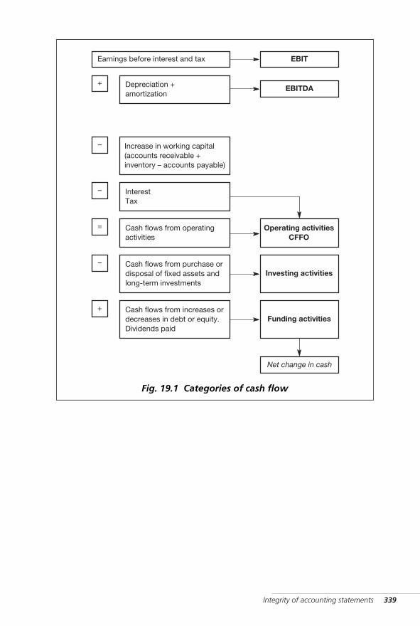
Integrity of accounting statements 339
InterestTax
Cash flows from operatingactivities
=
Depreciation +amortization
+
Earnings before interest and tax
Cash flows from purchase ordisposal of fixed assets andlong-term investments
Cash flows from increases ordecreases in debt or equity.Dividends paid
+
EBIT
EBITDA
Operating activitiesCFFO
Investing activities
Funding activities
Net change in cash
Increase in working capital(accounts receivable +inventory – accounts payable)
Fig. 19.1 Categories of cash flow
WKMR_CH19.QXD 11/24/05 12:49 PM Page 339
So we segregate cash flow into its three major activities:
■ cash flow from operations (CFFO)■ cash flow from investments■ cash flow from funding.
CFFO versus net income
We would expect over time to see a relationship between CFFO and netearnings. They should show similar rates of growth over time. If this rela-tionship is solid it tends to be a sign of good health. However, if asignificant divergence emerged between the trends in these two variablesit could indicate that the reporting of earnings is being artificiallyinflated, that aggressive accounting measures are being used to cover upfundamental problems.
One way to inflate earnings is to create premature or fictitious revenue.However, neither of these kinds of revenue generate any extra cash.Therefore even though a company can report extra revenue it cannotreport extra cash in-flow.
Similarly when a company indulges in aggressive cost capitalization itmoves items of expense from the profit and loss account onto the balancesheet, thereby reporting extra profit. Cash however has been paid out inrespect of these expenses and whereas moving the expense to the balancesheet will result in increased profit it will not result in increased cashflow. Likewise we can boost declared profit by reducing a reserve account,but this again will not boost cash flow, and so on.
In the figure for CFFO therefore we have a further tool to test theintegrity of financial accounts.
340 Key management ratios
✓
To repeat: cash flow from operations is a truly significant number. If we can imag-ine the company’s production and selling operations as an electric generator, thecash flow from operations is the electrical power output from this generator thatis both continuous and sustainable. The other forms of cash flow, i.e. investingand funding, do not have these powerful characteristics. Much of a company’svalue therefore lies in the strength of its CFFO.
%
!
☛
WKMR_CH19.QXD 11/24/05 12:49 PM Page 340
Introduction
Values taken from company accounts are used to analyze business per-formance. For the vast bulk of these values there are no quibbles abouttheir accuracy or realism. However, there are some items that are subjectto a number of different interpretations. Whether one interpretation ispreferred over another will affect the results of the analysis. A multitudeof rules laid down by the accounting bodies, the statutory authorities, theStock Exchange and others have a bearing in these interpretations. Someunderstanding of the more important of these rules provides a usefulbackground to analysis.
The principle underlying the rules may be even more important. Theoverriding principle is the ‘true and fair view’ that accounts should pres-ent. This said, it is often difficult to draw up rules for specific items thatwill always reflect a true and fair view. It is for this reason that differentinterpretations can arise to give different answers to our analysis.
As external conditions change, the emphasis moves to different aspectsof the accounts – from the profit and loss account to the balance sheet tothe cash flow. New problems, such as fluctuating currencies, give rise tothe need for new rules and so on. This appendix will address some of themore important ‘live’ issues in accounting at the present time. It willexplain why they are live, what the current state of play is and how differ-ent methods of treatment would affect the analysis.
These issues are:
■ goodwill ■ foreign currencies ■ pensions ■ deferred tax ■ leases ■ revaluation of fixed assets ■ scrip issues ■ miscellaneous long funds■ EBITDA■ terminal value – SVA.
Appendix 1: Special items 341
Appendix 1: Special items
✓
WKMR_Z01.QXD 11/24/05 1:12 PM Page 341
Goodwill on acquisition
When one company acquires another for a price (consideration) in excessof the fair value of its net assets, goodwill is created. This goodwill amountwill appear not in the accounts of either the buyer or vendor, but in the con-solidated, or, combined accounts of the two companies. Goodwill is called anintangible asset, that is an asset of no physical substance. In many ratios,calculations are based on tangible assets only, thus totally ignoring good-will. Nevertheless, it has important effects on a company’s reportedposition and so an understanding of its origins and treatment is important.
First we will look at a non-goodwill situation called Scenario 1 in FigureA1.1. It will serve as a base position from which to work towards a good-will example.
Company A has paid $100 for Company B, the balance sheet for whichis shown with a net worth of $100. The entries that appear in CompanyA’s balance sheet are ‘Investment $100’ and the investment is balancedby an equivalent long-term loan.
When we look at the consolidated balance sheet for Scenario 1 the item‘Investment $100’ has disappeared. The values in the following boxesare combined:
■ fixed assets ■ current assets ■ current liabilities ■ long-term loans.
The ordinary funds of Company A are unchanged in the consolidated bal-ance sheet. Also, before consolidation, the total assets were $1000 for Aand $400 for B. The combined statement is in balance with its total assetsbeing equal to the sum of the two separate companies less the Company A$100 investment and Company B ordinary funds deducted from each side.
When we consider what has happened, we see that the investment of$100 in Company A’s balance sheet has simply been replaced by netassets of $100 ($400 assets – $300 liabilities) from Company B.
In practice, the question of ‘fair value’ of both assets acquired and consider-ation given would arise. It has been assumed that this is not an issue here.
342 Key management ratios
%
WKMR_Z01.QXD 11/24/05 1:12 PM Page 342
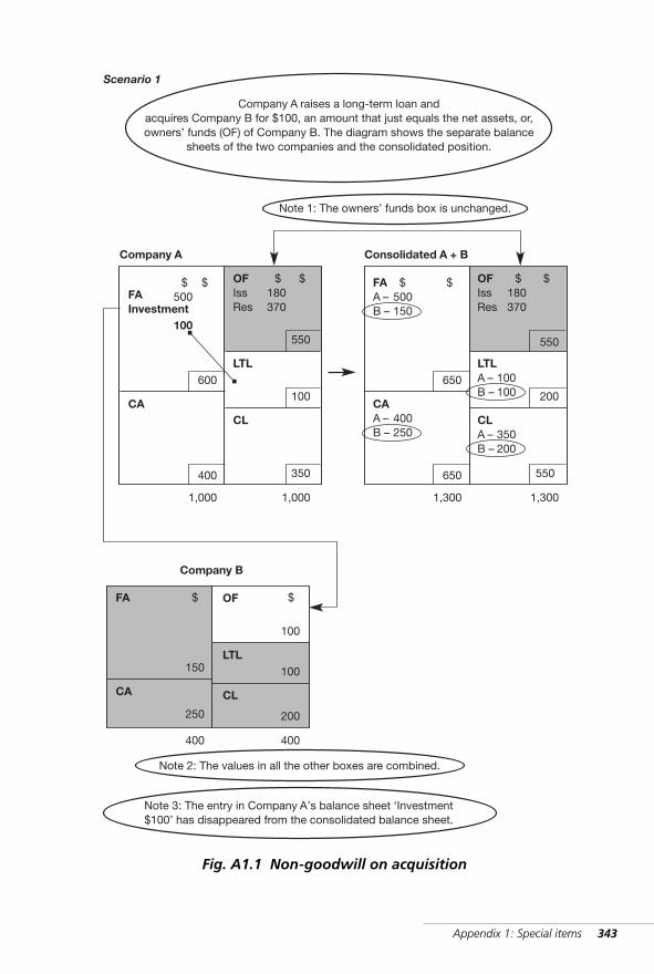
Appendix 1: Special items 343
Company A raises a long-term loan andacquires Company B for $100, an amount that just equals the net assets, or,owners’ funds (OF) of Company B. The diagram shows the separate balance
sheets of the two companies and the consolidated position.
FAInvestment
CA
OFIssRes
LTL
CL
180370
$
550
$
100
350
1,000
500
100
$
600
$
400
1,000
FAA –B –
CAA –B –
LTLA –B –
CLA –B –
550
200
550
1,300
500150
$
650
$
650
1,300
100100
350200
400250
Company A Consolidated A + B
OFIssRes
180370
$
FA
CA
OF
LTL
CL
100
100
200
400
150
250
400
Company B
Note 1: The owners’ funds box is unchanged.
Note 2: The values in all the other boxes are combined.
Note 3: The entry in Company A’s balance sheet ‘Investment$100’ has disappeared from the consolidated balance sheet.
550
$
$$
Scenario 1
Fig. A1.1 Non-goodwill on acquisition
WKMR_Z01.QXD 11/24/05 1:12 PM Page 343
A goodwill acquisition
In Scenario 2 in Figure A1.2, the amount paid by Company A forCompany B is $125. Company B is the same firm as in Scenario 1, whosenet assets are $100. On consolidation, the extra consideration of $25 isnot balanced by physical assets so an intangible asset of this amount mustbe created. The name we give to this intangible asset is goodwill. (The jus-tification for a high acquisition price and, therefore, the goodwill element,exists in the mind of the buyer, but, logically, it has to be the expectationof extra future profit.)
Three ways of treating goodwill are:
■ by annual charges to the profit and loss account – it can bedepreciated in just the same way as any fixed assets and it will, intime, disappear from the accounts (this way out is not favoured bybusiness people because its effect is to reduce declared profit, whichwill be reflected in the earnings per share figure and other measuresof performance).
■ by an immediate charge against reserves – assets may bereduced by the amount of goodwill and reserves by the same amountso, at a single stroke, goodwill simply disappears, totally (in theconsolidated balance sheet shown in Figure A1.2, reserves of $370would be reduced by $25 to $345, reported ordinary funds would fallby $25 to $525 and balance sheet totals go down to $1300).
■ by write-off of any impairment of value – as reflected incurrent forecasts of operations.
The effect of the second treatment is that profits are not affected and var-ious balance sheet totals are reduced. Because of higher profits and lowerassets the profitability ratios of return on total assets and return onequity will look better. The debt/equity ratio, though, will look worsebecause equity funds are artificially reduced. It is likely that the highreturn on total assets, return on equity, and market to book ratios in thesample companies are partly attributable to this treatment of goodwill.
344 Key management ratios
Once consideration in cash or other assets is given for goodwill a number ofquestions then arise:
■ ‘How is it treated in the accounts?’
■ ‘How will different ways of treating it affect our analysis?’
?
☛
WKMR_Z01.QXD 11/24/05 1:12 PM Page 344
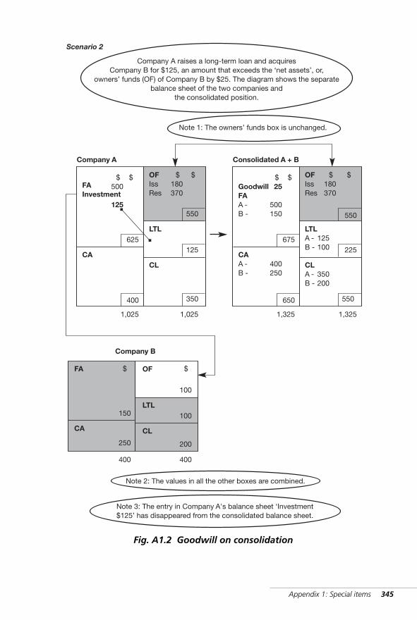
Appendix 1: Special items 345
Company A raises a long-term loan and acquiresCompany B for $125, an amount that exceeds the ‘net assets’, or,
owners’ funds (OF) of Company B by $25. The diagram shows the separatebalance sheet of the two companies and
the consolidated position.
FAInvestment
CA
OFIssRes
LTL
CL
180370
$
550
$
125
350
1,025
500
125
$
625
$
400
1,025
GoodwillFAA -B -
CAA -B -
LTLA -B -
CLA -B -
550
225
550
1,325
500150
$
675
$
650
1,325
125100
350200
400250
Company A Consolidated A + B
OFIssRes
180370
$
FA
CA
OF
LTL
CL
100
100
200
400
150
250
400
Company B
Note 1: The owners’ funds box is unchanged.
Note 2: The values in all the other boxes are combined.
Note 3: The entry in Company A's balance sheet ‘Investment$125’ has disappeared from the consolidated balance sheet.
550
$
$$
Scenario 2
25
Fig. A1.2 Goodwill on consolidation
WKMR_Z01.QXD 11/24/05 1:12 PM Page 345
Foreign currency
Movements in exchange rates affect company performance in variousways, principally by way of transactions in the profit and loss account andholdings of overseas assets and liabilities in the balance sheet. We oftennote that an increase in the value of sterling will cause a weakening in theshare price of companies with substantial foreign interests, and vice versa.
In general, gains and losses arising from foreign currency exchange ratemovements are treated as follows:
■ profit and loss transactions are translated at average currencyvalues for the year
■ assets and liabilities in the closing balance sheet are translated atrates that applied at the date of the final accounts
■ net assets of the opening balance sheet are restated at the closingrates, the difference from the previous year being taken to reserves
■ exchange differences on foreign currency borrowings directly raisedfor, or to provide a hedge against, overseas fixed assets are taken toreserves and offset against the exchange differences on the assets
■ all other gains and losses are passed through the profit and lossaccount.
Pensions
Capital sums invested in pension funds and annual contributions havegrown so large that they can have a bearing on company performance.The pension funds themselves should not directly impinge on a com-pany’s accounts because they are separate funds totally independent ofcompany finances. However, the liability of a company to provide foremployees’ pensions means that a shortfall in the fund has to be filled byincreased annual contributions. Likewise, a surplus can allow the com-pany to take a holiday from contributions, thereby improving its cashflow and profit results. The surplus or deficit on the fund is, therefore, ofsupreme importance to the value of the company.
346 Key management ratios
☛
WKMR_Z01.QXD 11/24/05 1:12 PM Page 346
Deferred tax
The amount of tax charged in company accounts is often considerably dif-ferent from the actual tax paid. This arises from ‘timing differences thatare likely to reverse in the foreseeable future’. Behind this phrase lies gov-ernment legislation. To encourage investment in fixed assets, manygovernments give accelerated capital allowances on new plant. They allow ahigher charge against profits for the writing down of the fixed assets thanwould be justified on the basis of a straightforward depreciation calculation.
The result to the company is a lower tax charge in the early years of aninvestment. However, if excess amounts are taken for depreciation earlyin the life of plant, there is none left for later years. The result will beheavier tax charges in these latter years. It is accepted that, for businesspurposes, this artificial distortion of reported profits is better avoided.Accordingly, in the early years, the full tax charge is made in the accountsand the amount not paid is put to the deferred tax account. It will bedrawn down in later years. However, this said, a certain amount is left tothe discretion of management to determine how much of a charge is‘likely to crystallize in the foreseeable future’.
Finance leases
Assets in the balance sheet include only items that are owned by the com-pany. At least, this was the fundamental rule until quite recently when aconsiderable amount of off-balance sheet financing came into use. By thisphrase is meant that assets were being acquired which were funded byloans, but neither the asset nor the loan appeared in the accounts. Inlegal terms, these assets were leased, but all the risks and rewards ofownership accrued to the company. The term finance lease is now used inthis situation to distinguish it from the ordinary operating lease. With afinance lease, both the asset and the funding must appear in the accounts.
Appendix 1: Special items 347
WKMR_Z01.QXD 11/24/05 1:12 PM Page 347
Revaluation of fixed assets
High rates of inflation over two decades had resulted in a situation wherethe values for property in company accounts were far removed from real-ity. It was accepted that it was necessary to remove this anomaly andfixed assets were allowed to be shown at valuation rather than at cost.
Our interest here is to consider the effect of revaluation on the variousbusiness ratios. First we will look at the accounting treatment that isillustrated in Figure A1.3. The increase in value of the fixed assets ismatched by an increase in reserves.
Balance sheet values for fixed assets, total assets and ordinary funds areincreased. The impact on business ratios is exactly the opposite to that whichresulted from the writing off of goodwill shown earlier in this appendix.
The debt/equity ratio improves, as does the asset backing per share.However, return on total assets and return on equity will worsen. For ananalysis of accounts for a series of years, spurious movements in ratioscan arise simply from revaluation.
The best way to eliminate these is to back-date the revaluation to thestart of the analysis period.
348 Key management ratios
☛
WKMR_Z01.QXD 11/24/05 1:12 PM Page 348
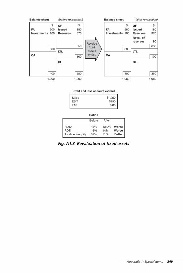
Appendix 1: Special items 349
600
400
550
350
100
Balance sheet (before revaluation)
FAInvestments
500100
$ OFIssuedReserves
180370
$
LTL
CL
CA
1,000 1,000
680
400
630
350
100
Balance sheet (after revaluation)
FAInvestments
580100
$ OFIssuedReserves
180370
$
Reval. ofreserves 80
LTL
CL
CA
1,080 1,080
Revaluefixed
assetsby $80
Profit and loss account extract
SalesEBITEAT
$1,250$150$ 88
Ratios
ROTAROETotal debt/equity
15%16%82%
Before
13.9%14%71%
After
WorseWorseBetter
Fig. A1.3 Revaluation of fixed assets
WKMR_Z01.QXD 11/24/05 1:12 PM Page 349
Scrip issue
A scrip, or, bonus issue takes place when shareholders in a company aregiven extra free shares in proportion to their existing holdings. Forinstance in a one-for-two scrip, all shareholders will have their number ofshares increased by 50 percent. From a ratio point of view, this has aneffect on EPS, DPS, assets per share and, normally, market price pershare. The historic values must all be moved down in proportion to theincrease in number of shares.
In Figure A1.4 we show an example of a company that made a one-for-two scrip issue. From a base of 180 shares, it issued 90 extra shares freeto its existing shareholders. It also transferred $90 from reserves toissued capital. The pre-scrip market price was $4.80. What is the likelypost-scrip market price?
Does a scrip bring real benefit to the shareholder? The logic is that thereshould be no change in their overall position: they own the same fraction ofthe company after the scrip as before and the total value of the companyhas not increased. However, in practice, a scrip is a buoyant signal to themarket that may improve a share’s value. The accounting entry is simply atransfer from reserves to issued capital, as shown in Figure A1.4.
350 Key management ratios
WKMR_Z01.QXD 11/24/05 1:12 PM Page 350
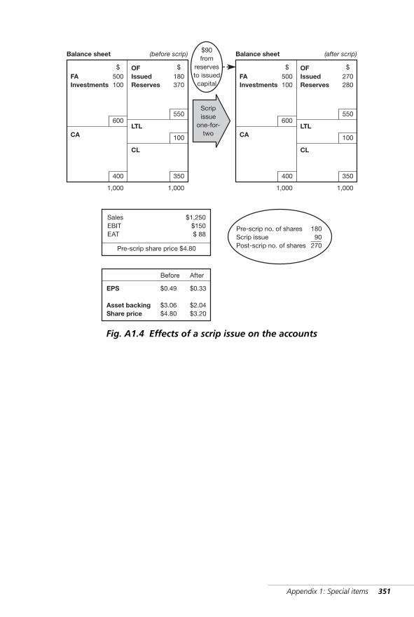
Appendix 1: Special items 351
Balance sheet (before scrip)
Scripissue
one-for-two
Pre-scrip share price $4.80
SalesEBITEAT
$1,250$150$ 88
EPS
Asset backingShare price
$0.49
$3.06$4.80
Before
$0.33
$2.04$3.20
After
Balance sheet (after scrip)$90from
reservesto issuedcapital
600
400
FAInvestments
500100
$
CA
1,000
550
350
100
OFIssuedReserves
180370
$
LTL
CL
1,000
550
350
100
OFIssuedReserves
270280
$
LTL
CL
1,000
600
400
FAInvestments
500100
$
CA
1,000
Pre-scrip no. of sharesScrip issuePost-scrip no. of shares
18090
270
Fig. A1.4 Effects of a scrip issue on the accounts
WKMR_Z01.QXD 11/24/05 1:12 PM Page 351
Miscellaneous long-term funds
In chapter 1 it was mentioned that certain items do not fit comfortably intothe structure of the five-box balance sheet. These items have been ignoredthroughout the analysis in this book because, in many companies, theseitems do not exist at all and in most others, they are of little importancefrom a financial analysis point of view.
However, they are mentioned here as an aside so that when they areencountered they can be dealt with appropriately. Under the heading‘Miscellaneous long-term funds’, they lie between ordinary funds andlong-term loans.
Preference shares
Preference shareholders, paradoxically, have very limited rights. They arepart-owners and receive a dividend at a fixed percent before the ordinaryshareholder. At one time this was a popular form of funding, but it is nowused in very limited and special circumstances. It may be for tax planningor voting control purposes for example. Preference shares will often haveconversion rights into ordinary shares and, if so, they can be included withthat category. For debt/equity ratio purposes, they can be treated as equity.
Minority interests
This entry occurs when the consolidated group includes subsidiaries thatare less than 100 percent owned. They are equity funds but not part ofthe group’s equity. Usually the amount is insignificant, but, for calculat-ing the debt/equity ratio, they could, again, be included with equity.
Deferred tax, grants and miscellaneous provisions
Deferred tax has been discussed above. It is probably best treated as an‘interest-free loan’ from the government and, therefore, included as debt.Grants will, in due course, move up into equity. Miscellaneous provisionscould be pension funds not fully covered; they are neither debt nor equity.Both items can be ignored in the balance sheet ratios unless the amountsare significant.
352 Key management ratios
☛
WKMR_Z01.QXD 11/24/05 1:12 PM Page 352
EBITDA
EBITDA (earnings before interest, tax, depreciation and amortization) isthe newest financial term to come into common use over recent years. Itidentifies cash flow measured at one particular point in the overall cash-flow cycle.
In order to identify its component parts we will first look at EBIT – earn-ings before interest and tax. We have seen in chapter 4 that EBIT is the firstimportant measure of profit that we identify in a profit and loss account.
It is largely the operating or trading profit of the business (there may beminor adjustments for non-operating income, etc.). Therefore EBIT cap-tures the total operating income and total operating cost of the business.
It is a number of enormous significance because it is from EBIT that acompany generates resources to pay interest to bankers, tax to the gov-ernment, dividends to shareholders, and, maybe even repay loans, etc.And in most companies it represents an ongoing, continuous source ofrenewable energy.
However, it is a number that is produced according to certain account-ing rules, one of these rules relates to the charge that we make fordepreciation. We have seen in chapter 8 the role that depreciation plays inlinking profit from trading with cash flow from the same source.Depreciation, which is a non-cash cost, must be excluded from the cashflow calculation.
Amortization is the term we use in relation to the writing down ofgoodwill. For the moment we can consider it as simply depreciation underanother name, i.e. a non-cash charge in the profit and loss account.
We add back both depreciation and amortization to EBIT to getEBITDA. It represents the cash that is thrown off from the normal trad-ing activities of the business (before any provision has been made forreinvestment in fixed assets, working capital, etc.). It may also beadjusted for certain non-recurring, non-operating items that have beencharged prior to EBIT.
After we separate out any discontinued operations, we can say thatEBITDA identifies the sustainable and hopefully growing stream of cashthat will flow from the trading activities of the business over the comingyears, and it is a number that is largely free from some distortions thatcan arise from accounting policies. Operating managers and analysts likeit for this reason.
We have said that amortization can be considered as another form ofdepreciation, but there is a significant difference between these twocharges. Depreciation is a true cost related to the passage of time, eventhough it is not a cash cost in the current period. The fact that machinesdo wear out over time and have to be replaced has to be recognized in theaccounts.
Amortization of goodwill, however, is a far more contentious issue. It isdifficult to support the theory that it gradually wears out over time.
Appendix 1: Special items 353
WKMR_Z01.QXD 11/24/05 1:12 PM Page 353
We can say that goodwill is the premium that one company will pay toacquire the assets of another that appears to have the capacity to earnabove normal profits. The inherent value of this goodwill can change as aresult of many factors, it can remain constant, it can even grow. It can dis-appear overnight as we have seen in the cases of telecom companies thathave been taken over at extraordinary high premiums.
Therefore, if we decide to write it down by an annual charge over afixed period of time, just as if we were writing off a regular depreciatingfixed asset, we should recognize that this is an artificial charge and allowfor that fact in our financial reporting.
Terminal value calculation in the SVA model
The revised method (shown in chapter 17, page 289) for calculating theterminal value of a company some years ahead illustrated one particularapproach which we call the ‘annuity’ method. In this approach we take aparticular cash flow, i.e. NOPAT, and we capitalize it simply by dividing bythe cost of capital, WACC.
It is logical and correct to do this when we know or can assume thatthis is a constant cash flow that will persist for a long, indefinite periodinto the future.
Provided certain conditions are met, this approach to valuation is cor-rect even if the cash flow is not constant but growing. The mostimportant condition here is that the return generated by the company, i.e.ROIC, is exactly equal to its cost of funds, i.e. WACC.
When this condition applies then the benefits of growth in the cashflow will be entirely absorbed by the extra capital required to support thegrowing business. Because all the benefits of this growth are cancelled outwe can ignore it and use a method of valuation that is based on a constantcash flow.
There are strong economic arguments in favor of this approach, butthere are also many who argue cogently that growth into the long-termfuture does have an impact on value and must be allowed for.
In favor of the former position is the economic case that a companythat earns profits in excess of the cost of capital will attract competitionfrom new entrants to the market who wish to share in those excess prof-its. This competition will reduce profitability in the market sector. Newentrants will continue to be attracted until overall profitability falls to theexact level of the cost of funds, at which stage the equilibrium is reached.
Proponents of the latter position argue that a large, well-established,well-managed company has a competitive advantage over any newentrants, and such companies can sustain indefinitely a rate of profit con-siderably in excess of the cost of capital. If this latter proposition isaccepted, the annuity approach that we have used in chapter 17 under-states the continuing value of the company, and we have to use a newformula which is difficult but more accurate. See opposite.
354 Key management ratios
WKMR_Z01.QXD 11/24/05 1:12 PM Page 354
Formula to establish the terminal value of a company with growth in acompetitive advantage situation.
[NOPAT(t+1) * (1 – g/r)]/(WACC – g)
What this formula says is that we start with final year NOPAT, and wemove it forward one year at the expected growth rate, i.e. NOPAT(t+1).
We multiply this value by (1 – g/r). The symbol ‘g’ stands for expectedgrowth rate, and ‘r’ stands for the company’s rate of return.
Let us say that g = 8% and r = 12%. We multiply by (1 – 8/12) whichreduces NOPAT to 33% of its original value.
We then divide this number by (WACC – g). Growth has already beenfixed at 8%. Let us say that WACC equals 10%. The values within brack-ets are therefore (10% – 8%) which gives us 2%.
We will work out the values by the two different methods for a hypotheti-cal company with a NOPAT of $100.
Annuity approach
TV = NOPAT/WACC= $100/.10= $1000
Long-term growth approach
TV = [NOPAT(t+1) * (1 – g/r)]/(WACC – g)= [($100 * 1.08) * (1 – 8/12)]/(.10–.08)= $1782
This second approach has resulted in a much higher value. This value isheavily influenced by the growth rate. The reader may like to check thatan assumed growth rate of 4% would give a value much closer to theannuity value, i.e. $1,144.
Appendix 1: Special items 355
WKMR_Z01.QXD 11/24/05 1:12 PM Page 355
Abbott Laboratories Lowe’s Companies, Inc.Albertson’s Inc. Merck & Co, Inc.Amgen Inc. Parker-Hannifin CorporationBaxter, Inc. Pfizer Inc.Bristol-Myers Squibb Co. Pharmacia CorporationCampbell Soup Company Pitney Bowes Inc.Caterpillar Inc. Ralston Puri GroupCoGra Foods Incorporated Safeway Inc.Colgate-Palmolive Co. Sara Lee CorporationCostco Wholesale Corporation Schering-Plough CorporationCvs Corporation Stanley WorksDeere & Co. Target CorporationDover Corporation The Gap, Inc.Eli Lilly and Company The Gillette CompanyHershey Foods Corporation The Kroger Co.Home Depot Inc. The May Department Stores Co.Ingersoll-Rand Company Walgreen Co.Johnson & Johnson Wal-Mart Stores Inc.Kellogg Co. William Wrigley Jr CompanyLexmark, International, Inc.
356 Key management ratios
Appendix 2: Companiesused in the sample
United States
United Kingdom
Alvis plc Cadbury Schweppes plcAmersham plc Carpetright plcAndrews Sykes Group plc Dairy Crest Group plcArriva plc De La Rue plcAsda Group plc Dfs Furniture Company plcAstrazeneca plc Dixon Motors plcBrake Bros. plc Domnick Hunter Group plcBrown & Jackson plc Express Dairies plc
WKMR_Z02.QXD 11/24/05 12:50 PM Page 356
Findel plc Richmond Foods plcGalen Holdings plc Safeway plcGeest plc Shiloh plcGlaxo Wellcome plc Shire Pharmaceuticals Group plcGlaxosmithkline plc Smith & Nephew plcGoldshield Group plc Smithkline Beecham plcGreggs plc Spirax-Sarco Engineering plcGus plc Ssl Inter. plcHalma plc Sterling Industries plcHewden Stuart plc T & S Stores plcHuntleigh Technology plc Tesco plcInter Link Foods plc Tex Holdings plcJJB Sports plc The Boots Company plcKingfisher plc The Carphone Warehouse Group plcLinx Printing Technologies plc The Weir Group plcLondon Inter. Group plc Thorntons plcMatalan plc Ti Group plcMedical Solutions plc Unilever plcN. Brown Group plc United Biscuits (Holdings) plcOxford Asymmetry Inter. plc Wt Foods plcPerkins Foods plc Wyevale Garden Centres plc
Appendix 2: Companies used in the sample 357
Altan Ag Karstadt Quelle AgArt’E’ Spa Klockner-Werke AktiengesellschaftBeiersdorf Ag L.D.C. Societe AnonymeBoiron Sa Lahmeyer AgBrioche Pasquier Legris Industries Societe AnonymeCarrefour L’OrealCasino, Guichard-Perrachon Et Cie Man Roland Druckmaschinen AgCastelgarden Spa Manitou Bf SaCastorama Dubois Investissements SCA Marion. ParfumeriesClarins Merck KgaaDanone Metro AgDe Dietrich & Cie Nestle Deutschland AgDuerr Ag Parmalat FiziariaEvialis Sa Printemps-La RedouteFleury Michon Promodes SaFonciere Euris Sa RallyeFresenius Ag Recordati Industria Chimica E FarmFresenius Medical Care Aktiengesel Roncadin SpaGuyenne Et Gascogne Sa Royal Canin SaHeidelberger Druckmaschinen Ag Sabaf SpAIndus Holding Ag Sanofi-SynthelaboIndustria Macchine Automatiche Spa Schering AktiengesellschaftIngenico-Compagnie Industrielle Schiapparelli 1824 SpaInterpump Group Spa UnibelIwka Ag Wella Ag
European Union
WKMR_Z02.QXD 11/24/05 12:50 PM Page 357
Ain Pharmaciez Inc. Meiji Dairies CorporationAjinomoto Co., Inc. Meiji Seika Kaisha Ltd.Amway Japan Ltd. Meiki Co., Ltd.Arrk Corporation Ministop Co., Ltd.Avon Products Company Ltd. Mitsubishi Kakoki Kaisha, Ltd.Banyu Pharmaceutical Co Ltd. Mitsukoshi Ltd.Belluna Co. Ltd. Nichiiko Pharmaceutical Co., Ltd.C&S Company Ltd. Nichirei CorporationCanon Inc. Nippon Conveyor Co., Ltd.Colin Corporation Nippon Meat Packers Inc.Daiki Engineering Co., Ltd. Nippon Suisan Kaisha Ltd.Disco Corporation Nisshin Seifun Group Inc.Ezaki Glico Co. Ltd. Nissin Food Products Co. Ltd.Fabrica Toyama Corporation Okk CorporationFancl Corporation Olympic CorporationFast Retailing Co., Ltd. Ono Pharmaceutical Co. Ltd.Fuji Machine Mfg. Co., Ltd. Paris Miki Inc.Fujisawa Pharmaceutical Co. Ltd. Ricoh Company, Ltd.Gasakiya Co., Ltd. (8262) Rohto Pharmaceutical Co., Ltd.Harmonic Drive Systems Inc. Ryohin Keikaku Co., Ltd.Hisamitsu Pharmaceutical Co., Inc. Santen Pharmaceutical CompanyHitachi Tool Engineering, Ltd. LimitedHoden Seimitsu Kako Kenkyusho Co., Seven-Eleven Japan Co. Ltd.Hogy Medical Co., Ltd. Shimamura Co., Ltd.Homac Corp. Smc CorporationHouse Foods Corporation Sodick Co., Ltd.Itoham Foods Inc. Ssp Company Ltd.Japan Cash Machine Co., Ltd. Sunkus & Associates Inc.Kao Corporation Suruga Seiki Co., Ltd.Katokichi Co. Ltd. Taisho Pharmaceutical Co. Ltd.Kawata Mfg. Co., Ltd. Takeda Chemical Industries, Ltd.Kikkoman Corporation Teikoku Electric Mfg. Co., Ltd.Koh. Shoji Co., Ltd. Tesec CorporationKojima Co., Ltd. Tokyo Seimitsu Co., Ltd.Komeri Co., Ltd. Torii Pharmaceutical Co., Ltd.Kose Corporation Toyo Suisan Kaisha, Ltd.Kotobukiya Company Limited Uht CorporationK’S Denki Corporation Union Tool Co.Lawson Inc. Valor Co., Ltd.Mandom Corporation Yakult Honsha Co. Ltd.Maruha Corporation Yamanouchi Pharmaceutical Co. Ltd.Matsumotokiyoshi Co., Ltd. Yushin Precision Equipment Co., Ltd.
Zeria Pharmaceutical Co., Ltd.
358 Key management ratios
Japan
WKMR_Z02.QXD 11/24/05 12:50 PM Page 358
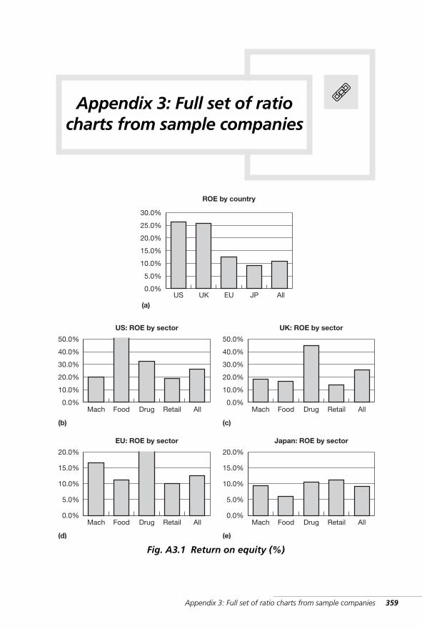
Appendix 3: Full set of ratio charts from sample companies 359
Appendix 3: Full set of ratiocharts from sample companies
20.0%
15.0%
10.0%
5.0%
0.0%
EU: ROE by sector
(d)
Mach Food Drug Retail All
20.0%
15.0%
10.0%
5.0%
0.0%
Japan: ROE by sector
(e)
Mach Food Drug Retail All
30.0%
15.0%
10.0%
5.0%
0.0%US
ROE by country
(a)UK EU JP All
25.0%
20.0%
50.0%
40.0%
30.0%
20.0%
10.0%
0.0%
US: ROE by sector
(b)
Mach Food Drug Retail All
50.0%
40.0%
30.0%
20.0%
10.0%
0.0%
UK: ROE by sector
(c)
Mach Food Drug Retail All
Fig. A3.1 Return on equity (%)
WKMR_Z03.QXD 11/24/05 12:50 PM Page 359
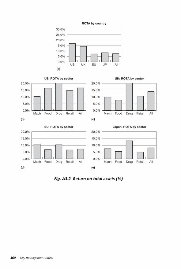
360 Key management ratios
20.0%
15.0%
10.0%
5.0%
0.0%
EU: ROTA by sector
(d)
Mach Food Drug Retail All
20.0%
15.0%
10.0%
5.0%
0.0%
Japan: ROTA by sector
(e)
Mach Food Drug Retail All
30.0%
15.0%
10.0%
5.0%
0.0%US
ROTA by country
(a)UK EU JP All
25.0%
20.0%
20.0%
15.0%
10.0%
5.0%
0.0%
US: ROTA by sector
(b)
Mach Food Drug Retail All
20.0%
15.0%
10.0%
5.0%
0.0%
UK: ROTA by sector
(c)
Mach Food Drug Retail All
Fig. A3.2 Return on total assets (%)
WKMR_Z03.QXD 11/24/05 12:50 PM Page 360
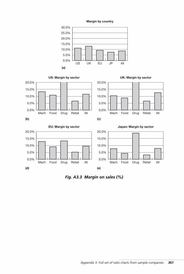
Appendix 3: Full set of ratio charts from sample companies 361
20.0%
15.0%
10.0%
5.0%
0.0%
EU: Margin by sector
(d)
Mach Food Drug Retail All
20.0%
15.0%
10.0%
5.0%
0.0%
Japan: Margin by sector
(e)
Mach Food Drug Retail All
30.0%
15.0%
10.0%
5.0%
0.0%US
Margin by country
(a)UK EU JP All
25.0%
20.0%
20.0%
15.0%
10.0%
5.0%
0.0%
US: Margin by sector
(b)
Mach Food Drug Retail All
20.0%
15.0%
10.0%
5.0%
0.0%
UK: Margin by sector
(c)
Mach Food Drug Retail All
Fig. A3.3 Margin on sales (%)
WKMR_Z03.QXD 11/24/05 12:50 PM Page 361
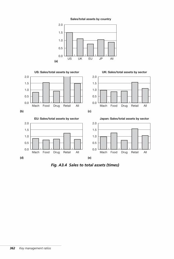
362 Key management ratios
2.0
1.5
1.0
0.5
0.0
EU: Sales/total assets by sector
(d)
Mach Food Drug Retail All
2.0
1.5
1.0
0.5
0.0
Japan: Sales/total assets by sector
(e)
Mach Food Drug Retail All
2.0
0.5
0.0US
Sales/total assets by country
(a)UK EU JP All
1.5
1.0
2.0
1.5
1.0
0.5
0.0
US: Sales/total assets by sector
(b)
Mach Food Drug Retail All
2.0
1.5
1.0
0.5
0.0
UK: Sales/total assets by sector
(c)
Mach Food Drug Retail All
Fig. A3.4 Sales to total assets (times)
WKMR_Z03.QXD 11/24/05 12:50 PM Page 362
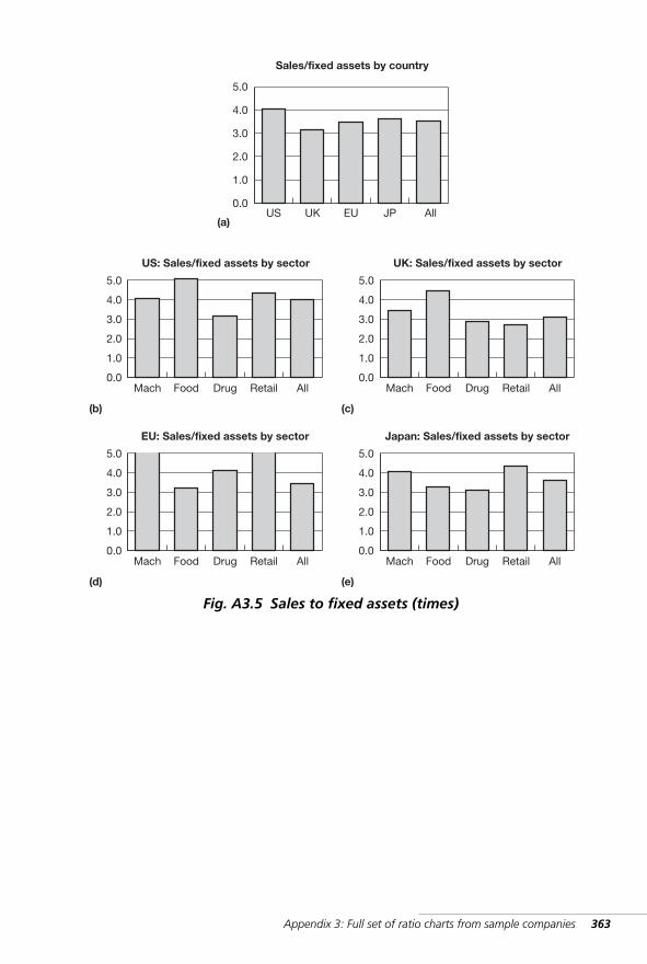
Appendix 3: Full set of ratio charts from sample companies 363
2.0
5.0
4.0
2.0
1.0
0.0
EU: Sales/fixed assets by sector
(d)
Mach Food Drug Retail All
5.0
4.0
3.0
1.0
0.0
Japan: Sales/fixed assets by sector
(e)
Mach Food Drug Retail All
5.0
1.0
0.0US
Sales/fixed assets by country
(a)UK EU JP All
3.0
2.0
5.0
4.0
2.0
1.0
0.0
US: Sales/fixed assets by sector
(b)
Mach Food Drug Retail All
5.0
4.0
2.0
1.0
0.0
UK: Sales/fixed assets by sector
(c)
Mach Food Drug Retail All
4.0
3.0 3.0
3.0
Fig. A3.5 Sales to fixed assets (times)
WKMR_Z03.QXD 11/24/05 12:50 PM Page 363
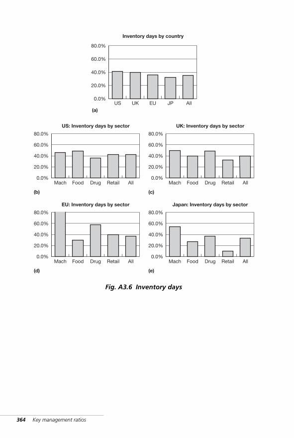
364 Key management ratios
80.0%
60.0%
40.0%
20.0%
0.0%
EU: Inventory days by sector
(d)
Mach Food Drug Retail All
80.0%
60.0%
40.0%
20.0%
0.0%
Japan: Inventory days by sector
(e)
Mach Food Drug Retail All
80.0%
20.0%
0.0%US
Inventory days by country
(a)UK EU JP All
60.0%
40.0%
80.0%
60.0%
40.0%
20.0%
0.0%
US: Inventory days by sector
(b)
Mach Food Drug Retail All
80.0%
60.0%
40.0%
20.0%
0.0%
UK: Inventory days by sector
(c)
Mach Food Drug Retail All
Fig. A3.6 Inventory days
WKMR_Z03.QXD 11/24/05 12:50 PM Page 364
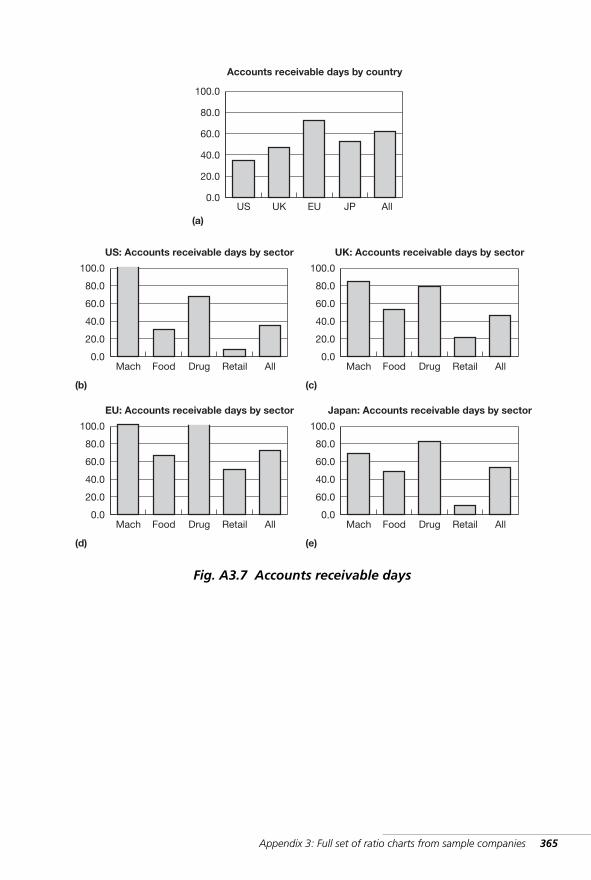
Appendix 3: Full set of ratio charts from sample companies 365
60.060.0
100.0
80.0
40.0
20.0
0.0
EU: Accounts receivable days by sector
(d)
Mach Food Drug Retail All
100.0
80.0
40.0
60.0
0.0
Japan: Accounts receivable days by sector
(e)
Mach Food Drug Retail All
100.0
40.0
20.0
0.0US
Accounts receivable days by country
(a)UK EU JP All
80.0
60.0
100.0
80.0
60.0
40.0
20.0
0.0
US: Accounts receivable days by sector
(b)
Mach Food Drug Retail All
100.0
80.0
60.0
40.0
20.0
0.0
UK: Accounts receivable days by sector
(c)
Mach Food Drug Retail All
Fig. A3.7 Accounts receivable days
WKMR_Z03.QXD 11/24/05 12:50 PM Page 365
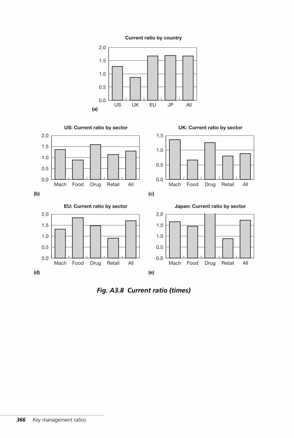
366 Key management ratios
2.0
1.5
1.0
0.5
0.0
EU: Current ratio by sector
(d)
Mach Food Drug Retail All
2.0
1.5
1.0
0.5
0.0
Japan: Current ratio by sector
(e)
Mach Food Drug Retail All
2.0
0.5
0.0US
Current ratio by country
(a)UK EU JP All
1.5
1.0
2.0
1.5
1.0
0.5
0.0
US: Current ratio by sector
(b)
Mach Food Drug Retail All
1.5
1.0
0.5
0.0
UK: Current ratio by sector
(c)
Mach Food Drug Retail All
Fig. A3.8 Current ratio (times)
WKMR_Z03.QXD 11/24/05 12:50 PM Page 366
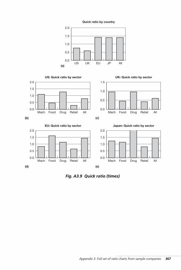
Appendix 3: Full set of ratio charts from sample companies 367
2.0
1.5
1.0
0.5
0.0
EU: Quick ratio by sector
(d)
Mach Food Drug Retail All
2.0
1.5
1.0
0.5
0.0
Japan: Quick ratio by sector
(e)
Mach Food Drug Retail All
2.0
0.5
0.0US
Quick ratio by country
(a)UK EU JP All
1.5
1.0
2.0
1.5
1.0
0.5
0.0
US: Quick ratio by sector
(b)
Mach Food Drug Retail All
1.5
1.0
0.5
0.0
UK: Quick ratio by sector
(c)
Mach Food Drug Retail All
Fig. A3.9 Quick ratio (times)
WKMR_Z03.QXD 11/24/05 12:50 PM Page 367
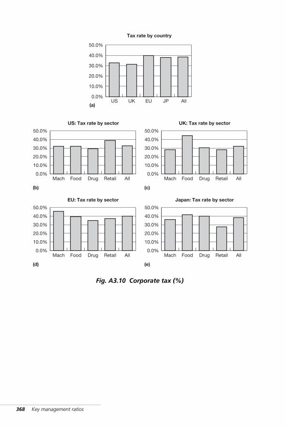
368 Key management ratios
20.0%
50.0%
40.0%
20.0%
10.0%
0.0%
EU: Tax rate by sector
(d)
Mach Food Drug Retail All
50.0%
40.0%
30.0%
10.0%
0.0%
Japan: Tax rate by sector
(e)
Mach Food Drug Retail All
50.0%
10.0%
0.0%US
Tax rate by country
(a)UK EU JP All
30.0%
20.0%
50.0%
40.0%
20.0%
10.0%
0.0%
US: Tax rate by sector
(b)
Mach Food Drug Retail All
50.0%
40.0%
20.0%
10.0%
0.0%
UK: Tax rate by sector
(c)
Mach Food Drug Retail All
40.0%
30.0% 30.0%
30.0%
Fig. A3.10 Corporate tax (%)
WKMR_Z03.QXD 11/24/05 12:50 PM Page 368
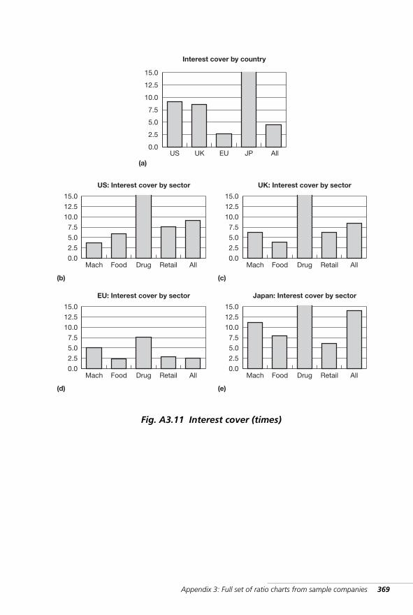
Appendix 3: Full set of ratio charts from sample companies 369
7.5
10.0
15.0
12.5
5.0
2.5
0.0
EU: Interest cover by sector
(d)
Mach Food Drug Retail All
15.0
12.5
5.0
2.5
0.0
Japan: Interest cover by sector
(e)
Mach Food Drug Retail All
15.0
7.5
5.0
2.5
0.0US
Interest cover by country
(a)UK EU JP All
12.5
10.0
15.0
12.5
10.0
7.5
2.5
0.0
US: Interest cover by sector
(b)
Mach Food Drug Retail All
15.0
12.5
7.5
5.0
2.5
0.0
UK: Interest cover by sector
(c)
Mach Food Drug Retail All
5.0
10.0 10.0
7.5
Fig. A3.11 Interest cover (times)
WKMR_Z03.QXD 11/24/05 12:50 PM Page 369
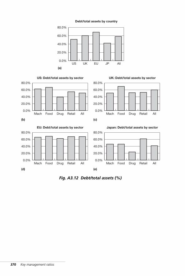
370 Key management ratios
80.0%
60.0%
40.0%
20.0%
0.0%
EU: Debt/total assets by sector
(d)
Mach Food Drug Retail All
80.0%
60.0%
40.0%
20.0%
0.0%
Japan: Debt/total assets by sector
(e)
Mach Food Drug Retail All
80.0%
20.0%
0.0%US
Debt/total assets by country
(a)UK EU JP All
60.0%
40.0%
80.0%
60.0%
40.0%
20.0%
0.0%
US: Debt/total assets by sector
(b)
Mach Food Drug Retail All
80.0%
60.0%
40.0%
20.0%
0.0%
UK: Debt/total assets by sector
(c)
Mach Food Drug Retail All
Fig. A3.12 Debt/total assets (%)
WKMR_Z03.QXD 11/24/05 12:50 PM Page 370
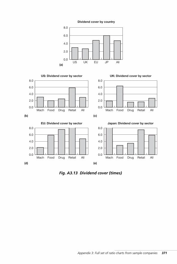
Appendix 3: Full set of ratio charts from sample companies 371
8.0
6.0
4.0
2.0
0.0
EU: Dividend cover by sector
(d)
Mach Food Drug Retail All
8.0
6.0
4.0
2.0
0.0
Japan: Dividend cover by sector
(e)
Mach Food Drug Retail All
8.0
2.0
0.0US
Dividend cover by country
(a)UK EU JP All
6.0
4.0
8.0
6.0
4.0
2.0
0.0
US: Dividend cover by sector
(b)
Mach Food Drug Retail All
8.0
6.0
4.0
2.0
0.0
UK: Dividend cover by sector
(c)
Mach Food Drug Retail All
Fig. A3.13 Dividend cover (times)
WKMR_Z03.QXD 11/24/05 12:50 PM Page 371
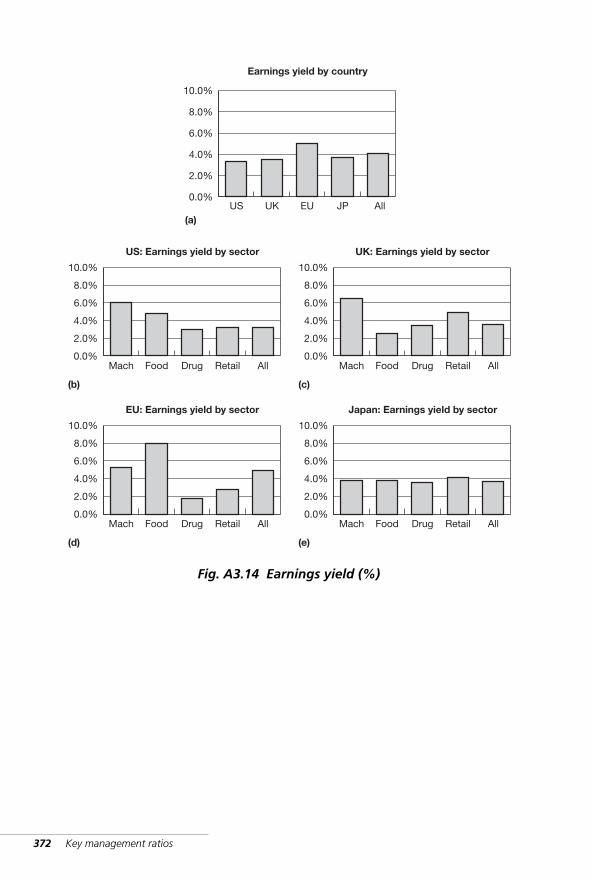
372 Key management ratios
6.0%6.0%
10.0%
8.0%
4.0%
2.0%
0.0%
EU: Earnings yield by sector
(d)
Mach Food Drug Retail All
10.0%
8.0%
4.0%
2.0%
0.0%
Japan: Earnings yield by sector
(e)
Mach Food Drug Retail All
10.0%
4.0%
2.0%
0.0%US
Earnings yield by country
(a)UK EU JP All
8.0%
6.0%
10.0%
8.0%
6.0%
4.0%
2.0%
0.0%
US: Earnings yield by sector
(b)
Mach Food Drug Retail All
10.0%
8.0%
6.0%
4.0%
2.0%
0.0%
UK: Earnings yield by sector
(c)
Mach Food Drug Retail All
Fig. A3.14 Earnings yield (%)
WKMR_Z03.QXD 11/24/05 12:50 PM Page 372
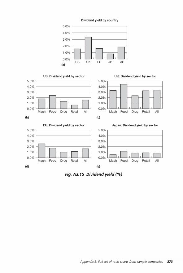
Appendix 3: Full set of ratio charts from sample companies 373
2.0%
5.0%
4.0%
2.0%
1.0%
0.0%
EU: Dividend yield by sector
(d)
Mach Food Drug Retail All
5.0%
4.0%
3.0%
1.0%
0.0%
Japan: Dividend yield by sector
(e)
Mach Food Drug Retail All
5.0%
1.0%
0.0%US
Dividend yield by country
(a)UK EU JP All
3.0%
2.0%
5.0%
4.0%
2.0%
1.0%
0.0%
US: Dividend yield by sector
(b)
Mach Food Drug Retail All
5.0%
4.0%
2.0%
1.0%
0.0%
UK: Dividend yield by sector
(c)
Mach Food Drug Retail All
4.0%
3.0% 3.0%
3.0%
Fig. A3.15 Dividend yield (%)
WKMR_Z03.QXD 11/24/05 12:50 PM Page 373
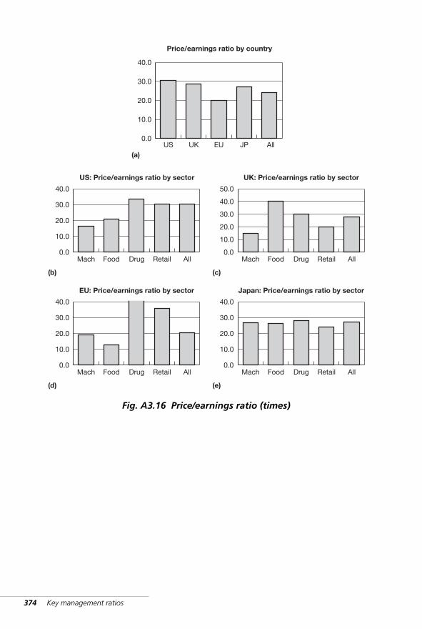
374 Key management ratios
30.0
40.0
30.0
20.0
10.0
0.0
EU: Price/earnings ratio by sector
(d)
Mach Food Drug Retail All
40.0
30.0
20.0
10.0
0.0
Japan: Price/earnings ratio by sector
(e)
Mach Food Drug Retail All
40.0
10.0
0.0US
Price/earnings ratio by country
(a)UK EU JP All
30.0
20.0
40.0
30.0
20.0
10.0
0.0
US: Price/earnings ratio by sector
(b)
Mach Food Drug Retail All
50.0
40.0
20.0
10.0
0.0
UK: Price/earnings ratio by sector
(c)
Mach Food Drug Retail All
Fig. A3.16 Price/earnings ratio (times)
WKMR_Z03.QXD 11/24/05 12:50 PM Page 374
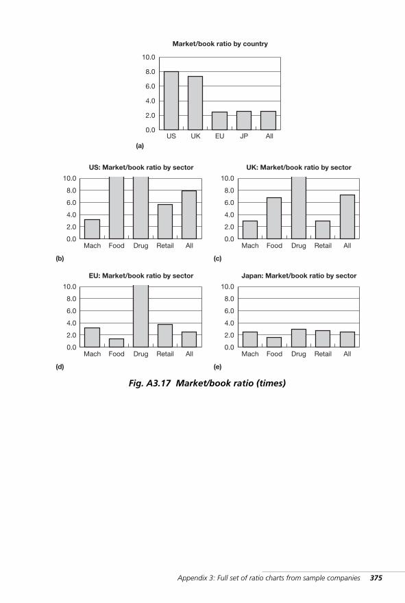
Appendix 3: Full set of ratio charts from sample companies 375
6.06.0
10.0
8.0
4.0
2.0
0.0
EU: Market/book ratio by sector
(d)
Mach Food Drug Retail All
10.0
8.0
4.0
2.0
0.0
Japan: Market/book ratio by sector
(e)
Mach Food Drug Retail All
10.0
4.0
2.0
0.0US
Market/book ratio by country
(a)UK EU JP All
8.0
6.0
10.0
8.0
6.0
4.0
2.0
0.0
US: Market/book ratio by sector
(b)
Mach Food Drug Retail All
10.0
8.0
6.0
4.0
2.0
0.0
UK: Market/book ratio by sector
(c)
Mach Food Drug Retail All
Fig. A3.17 Market/book ratio (times)
WKMR_Z03.QXD 11/24/05 12:50 PM Page 375
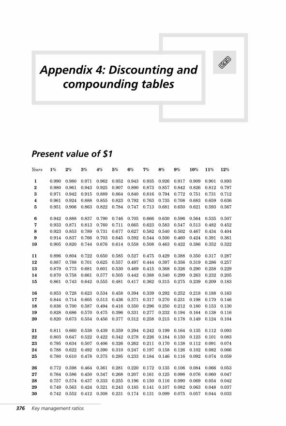
376 Key management ratios
Present value of $1
Years 1% 2% 3% 4% 5% 6% 7% 8% 9% 10% 11% 12%
1 0.990 0.980 0.971 0.962 0.952 0.943 0.935 0.926 0.917 0.909 0.901 0.8932 0.980 0.961 0.943 0.925 0.907 0.890 0.873 0.857 0.842 0.826 0.812 0.7973 0.971 0.942 0.915 0.889 0.864 0.840 0.816 0.794 0.772 0.751 0.731 0.7124 0.961 0.924 0.888 0.855 0.823 0.792 0.763 0.735 0.708 0.683 0.659 0.6365 0.951 0.906 0.863 0.822 0.784 0.747 0.713 0.681 0.650 0.621 0.593 0.567
6 0.942 0.888 0.837 0.790 0.746 0.705 0.666 0.630 0.596 0.564 0.535 0.5077 0.933 0.871 0.813 0.760 0.711 0.665 0.623 0.583 0.547 0.513 0.482 0.4528 0.923 0.853 0.789 0.731 0.677 0.627 0.582 0.540 0.502 0.467 0.434 0.4049 0.914 0.837 0.766 0.703 0.645 0.592 0.544 0.500 0.460 0.424 0.391 0.361
10 0.905 0.820 0.744 0.676 0.614 0.558 0.508 0.463 0.422 0.386 0.352 0.322
11 0.896 0.804 0.722 0.650 0.585 0.527 0.475 0.429 0.388 0.350 0.317 0.28712 0.887 0.788 0.701 0.625 0.557 0.497 0.444 0.397 0.356 0.319 0.286 0.25713 0.879 0.773 0.681 0.601 0.530 0.469 0.415 0.368 0.326 0.290 0.258 0.22914 0.870 0.758 0.661 0.577 0.505 0.442 0.388 0.340 0.299 0.263 0.232 0.20515 0.861 0.743 0.642 0.555 0.481 0.417 0.362 0.315 0.275 0.239 0.209 0.183
16 0.853 0.728 0.623 0.534 0.458 0.394 0.339 0.292 0.252 0.218 0.188 0.16317 0.844 0.714 0.605 0.513 0.436 0.371 0.317 0.270 0.231 0.198 0.170 0.14618 0.836 0.700 0.587 0.494 0.416 0.350 0.296 0.250 0.212 0.180 0.153 0.13019 0.828 0.686 0.570 0.475 0.396 0.331 0.277 0.232 0.194 0.164 0.138 0.11620 0.820 0.673 0.554 0.456 0.377 0.312 0.258 0.215 0.178 0.149 0.124 0.104
21 0.811 0.660 0.538 0.439 0.359 0.294 0.242 0.199 0.164 0.135 0.112 0.09322 0.803 0.647 0.522 0.422 0.342 0.278 0.226 0.184 0.150 0.123 0.101 0.08323 0.795 0.634 0.507 0.406 0.326 0.262 0.211 0.170 0.138 0.112 0.091 0.07424 0.788 0.622 0.492 0.390 0.310 0.247 0.197 0.158 0.126 0.102 0.082 0.06625 0.780 0.610 0.478 0.375 0.295 0.233 0.184 0.146 0.116 0.092 0.074 0.059
26 0.772 0.598 0.464 0.361 0.281 0.220 0.172 0.135 0.106 0.084 0.066 0.05327 0.764 0.586 0.450 0.347 0.268 0.207 0.161 0.125 0.098 0.076 0.060 0.04728 0.757 0.574 0.437 0.333 0.255 0.196 0.150 0.116 0.090 0.069 0.054 0.04229 0.749 0.563 0.424 0.321 0.243 0.185 0.141 0.107 0.082 0.063 0.048 0.03730 0.742 0.552 0.412 0.308 0.231 0.174 0.131 0.099 0.075 0.057 0.044 0.033
Appendix 4: Discounting andcompounding tables
WKMR_Z04.QXD 11/24/05 12:51 PM Page 376
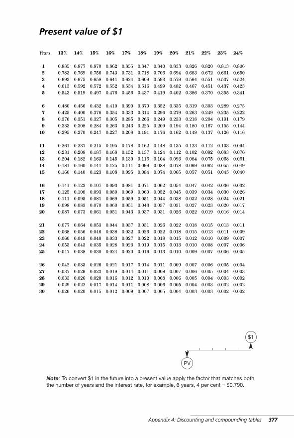
Appendix 4: Discounting and compounding tables 377
Present value of $1
Years 13% 14% 15% 16% 17% 18% 19% 20% 21% 22% 23% 24%
1 0.885 0.877 0.870 0.862 0.855 0.847 0.840 0.833 0.826 0.820 0.813 0.8062 0.783 0.769 0.756 0.743 0.731 0.718 0.706 0.694 0.683 0.672 0.661 0.6503 0.693 0.675 0.658 0.641 0.624 0.609 0.593 0.579 0.564 0.551 0.537 0.5244 0.613 0.592 0.572 0.552 0.534 0.516 0.499 0.482 0.467 0.451 0.437 0.4235 0.543 0.519 0.497 0.476 0.456 0.437 0.419 0.402 0.386 0.370 0.355 0.341
6 0.480 0.456 0.432 0.410 0.390 0.370 0.352 0.335 0.319 0.303 0.289 0.2757 0.425 0.400 0.376 0.354 0.333 0.314 0.296 0.279 0.263 0.249 0.235 0.2228 0.376 0.351 0.327 0.305 0.285 0.266 0.249 0.233 0.218 0.204 0.191 0.1799 0.333 0.308 0.284 0.263 0.243 0.225 0.209 0.194 0.180 0.167 0.155 0.144
10 0.295 0.270 0.247 0.227 0.208 0.191 0.176 0.162 0.149 0.137 0.126 0.116
11 0.261 0.237 0.215 0.195 0.178 0.162 0.148 0.135 0.123 0.112 0.103 0.09412 0.231 0.208 0.187 0.168 0.152 0.137 0.124 0.112 0.102 0.092 0.083 0.07613 0.204 0.182 0.163 0.145 0.130 0.116 0.104 0.093 0.084 0.075 0.068 0.06114 0.181 0.160 0.141 0.125 0.111 0.099 0.088 0.078 0.069 0.062 0.055 0.04915 0.160 0.140 0.123 0.108 0.095 0.084 0.074 0.065 0.057 0.051 0.045 0.040
16 0.141 0.123 0.107 0.093 0.081 0.071 0.062 0.054 0.047 0.042 0.036 0.03217 0.125 0.108 0.093 0.080 0.069 0.060 0.052 0.045 0.039 0.034 0.030 0.02618 0.111 0.095 0.081 0.069 0.059 0.051 0.044 0.038 0.032 0.028 0.024 0.02119 0.098 0.083 0.070 0.060 0.051 0.043 0.037 0.031 0.027 0.023 0.020 0.01720 0.087 0.073 0.061 0.051 0.043 0.037 0.031 0.026 0.022 0.019 0.016 0.014
21 0.077 0.064 0.053 0.044 0.037 0.031 0.026 0.022 0.018 0.015 0.013 0.01122 0.068 0.056 0.046 0.038 0.032 0.026 0.022 0.018 0.015 0.013 0.011 0.00923 0.060 0.049 0.040 0.033 0.027 0.022 0.018 0.015 0.012 0.010 0.009 0.00724 0.053 0.043 0.035 0.028 0.023 0.019 0.015 0.013 0.010 0.008 0.007 0.00625 0.047 0.038 0.030 0.024 0.020 0.016 0.013 0.010 0.009 0.007 0.006 0.005
26 0.042 0.033 0.026 0.021 0.017 0.014 0.011 0.009 0.007 0.006 0.005 0.00427 0.037 0.029 0.023 0.018 0.014 0.011 0.009 0.007 0.006 0.005 0.004 0.00328 0.033 0.026 0.020 0.016 0.012 0.010 0.008 0.006 0.005 0.004 0.003 0.00229 0.029 0.022 0.017 0.014 0.011 0.008 0.006 0.005 0.004 0.003 0.002 0.00230 0.026 0.020 0.015 0.012 0.009 0.007 0.005 0.004 0.003 0.003 0.002 0.002
Note: To convert $1 in the future into a present value apply the factor that matches boththe number of years and the interest rate, for example, 6 years, 4 per cent = $0.790.
$1
PV
WKMR_Z04.QXD 11/24/05 12:51 PM Page 377
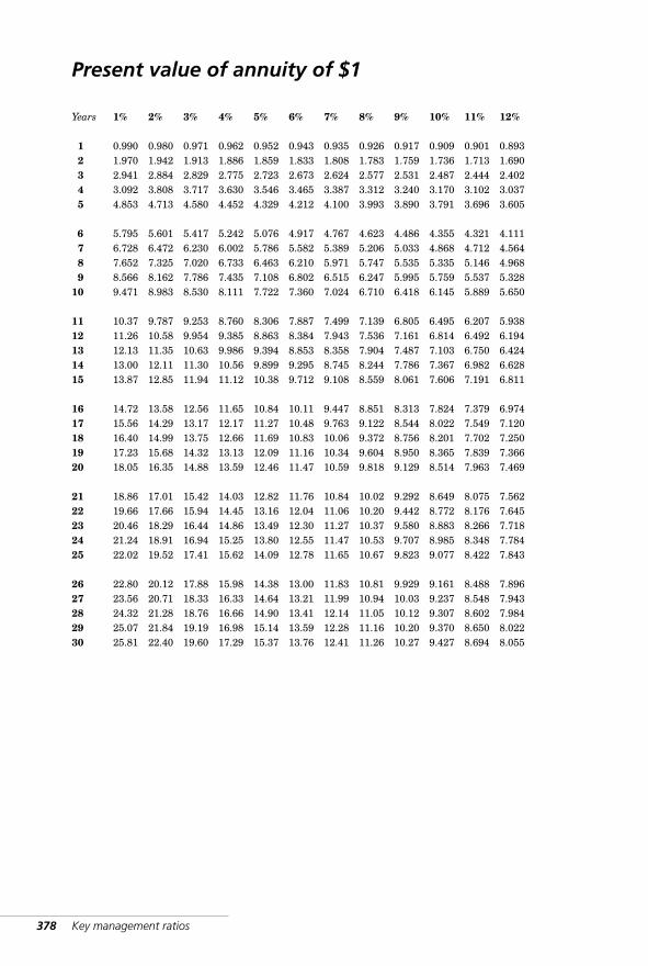
378 Key management ratios
Present value of annuity of $1
Years 1% 2% 3% 4% 5% 6% 7% 8% 9% 10% 11% 12%
1 0.990 0.980 0.971 0.962 0.952 0.943 0.935 0.926 0.917 0.909 0.901 0.8932 1.970 1.942 1.913 1.886 1.859 1.833 1.808 1.783 1.759 1.736 1.713 1.6903 2.941 2.884 2.829 2.775 2.723 2.673 2.624 2.577 2.531 2.487 2.444 2.4024 3.092 3.808 3.717 3.630 3.546 3.465 3.387 3.312 3.240 3.170 3.102 3.0375 4.853 4.713 4.580 4.452 4.329 4.212 4.100 3.993 3.890 3.791 3.696 3.605
6 5.795 5.601 5.417 5.242 5.076 4.917 4.767 4.623 4.486 4.355 4.321 4.1117 6.728 6.472 6.230 6.002 5.786 5.582 5.389 5.206 5.033 4.868 4.712 4.5648 7.652 7.325 7.020 6.733 6.463 6.210 5.971 5.747 5.535 5.335 5.146 4.9689 8.566 8.162 7.786 7.435 7.108 6.802 6.515 6.247 5.995 5.759 5.537 5.328
10 9.471 8.983 8.530 8.111 7.722 7.360 7.024 6.710 6.418 6.145 5.889 5.650
11 10.37 9.787 9.253 8.760 8.306 7.887 7.499 7.139 6.805 6.495 6.207 5.93812 11.26 10.58 9.954 9.385 8.863 8.384 7.943 7.536 7.161 6.814 6.492 6.19413 12.13 11.35 10.63 9.986 9.394 8.853 8.358 7.904 7.487 7.103 6.750 6.42414 13.00 12.11 11.30 10.56 9.899 9.295 8.745 8.244 7.786 7.367 6.982 6.62815 13.87 12.85 11.94 11.12 10.38 9.712 9.108 8.559 8.061 7.606 7.191 6.811
16 14.72 13.58 12.56 11.65 10.84 10.11 9.447 8.851 8.313 7.824 7.379 6.97417 15.56 14.29 13.17 12.17 11.27 10.48 9.763 9.122 8.544 8.022 7.549 7.12018 16.40 14.99 13.75 12.66 11.69 10.83 10.06 9.372 8.756 8.201 7.702 7.25019 17.23 15.68 14.32 13.13 12.09 11.16 10.34 9.604 8.950 8.365 7.839 7.36620 18.05 16.35 14.88 13.59 12.46 11.47 10.59 9.818 9.129 8.514 7.963 7.469
21 18.86 17.01 15.42 14.03 12.82 11.76 10.84 10.02 9.292 8.649 8.075 7.56222 19.66 17.66 15.94 14.45 13.16 12.04 11.06 10.20 9.442 8.772 8.176 7.64523 20.46 18.29 16.44 14.86 13.49 12.30 11.27 10.37 9.580 8.883 8.266 7.71824 21.24 18.91 16.94 15.25 13.80 12.55 11.47 10.53 9.707 8.985 8.348 7.78425 22.02 19.52 17.41 15.62 14.09 12.78 11.65 10.67 9.823 9.077 8.422 7.843
26 22.80 20.12 17.88 15.98 14.38 13.00 11.83 10.81 9.929 9.161 8.488 7.89627 23.56 20.71 18.33 16.33 14.64 13.21 11.99 10.94 10.03 9.237 8.548 7.94328 24.32 21.28 18.76 16.66 14.90 13.41 12.14 11.05 10.12 9.307 8.602 7.98429 25.07 21.84 19.19 16.98 15.14 13.59 12.28 11.16 10.20 9.370 8.650 8.02230 25.81 22.40 19.60 17.29 15.37 13.76 12.41 11.26 10.27 9.427 8.694 8.055
WKMR_Z04.QXD 11/24/05 12:51 PM Page 378
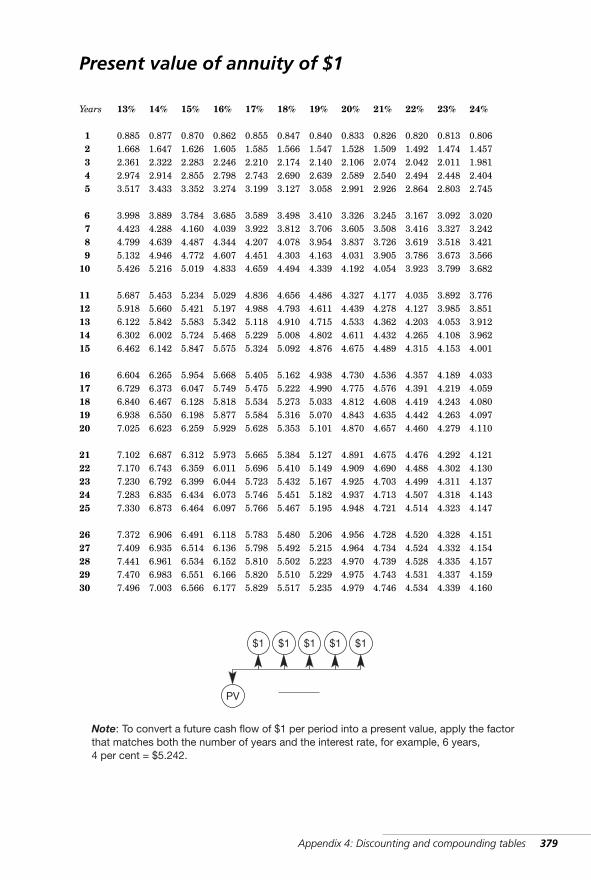
Appendix 4: Discounting and compounding tables 379
Present value of annuity of $1
Years 13% 14% 15% 16% 17% 18% 19% 20% 21% 22% 23% 24%
1 0.885 0.877 0.870 0.862 0.855 0.847 0.840 0.833 0.826 0.820 0.813 0.8062 1.668 1.647 1.626 1.605 1.585 1.566 1.547 1.528 1.509 1.492 1.474 1.4573 2.361 2.322 2.283 2.246 2.210 2.174 2.140 2.106 2.074 2.042 2.011 1.9814 2.974 2.914 2.855 2.798 2.743 2.690 2.639 2.589 2.540 2.494 2.448 2.4045 3.517 3.433 3.352 3.274 3.199 3.127 3.058 2.991 2.926 2.864 2.803 2.745
6 3.998 3.889 3.784 3.685 3.589 3.498 3.410 3.326 3.245 3.167 3.092 3.0207 4.423 4.288 4.160 4.039 3.922 3.812 3.706 3.605 3.508 3.416 3.327 3.2428 4.799 4.639 4.487 4.344 4.207 4.078 3.954 3.837 3.726 3.619 3.518 3.4219 5.132 4.946 4.772 4.607 4.451 4.303 4.163 4.031 3.905 3.786 3.673 3.566
10 5.426 5.216 5.019 4.833 4.659 4.494 4.339 4.192 4.054 3.923 3.799 3.682
11 5.687 5.453 5.234 5.029 4.836 4.656 4.486 4.327 4.177 4.035 3.892 3.77612 5.918 5.660 5.421 5.197 4.988 4.793 4.611 4.439 4.278 4.127 3.985 3.85113 6.122 5.842 5.583 5.342 5.118 4.910 4.715 4.533 4.362 4.203 4.053 3.91214 6.302 6.002 5.724 5.468 5.229 5.008 4.802 4.611 4.432 4.265 4.108 3.96215 6.462 6.142 5.847 5.575 5.324 5.092 4.876 4.675 4.489 4.315 4.153 4.001
16 6.604 6.265 5.954 5.668 5.405 5.162 4.938 4.730 4.536 4.357 4.189 4.03317 6.729 6.373 6.047 5.749 5.475 5.222 4.990 4.775 4.576 4.391 4.219 4.05918 6.840 6.467 6.128 5.818 5.534 5.273 5.033 4.812 4.608 4.419 4.243 4.08019 6.938 6.550 6.198 5.877 5.584 5.316 5.070 4.843 4.635 4.442 4.263 4.09720 7.025 6.623 6.259 5.929 5.628 5.353 5.101 4.870 4.657 4.460 4.279 4.110
21 7.102 6.687 6.312 5.973 5.665 5.384 5.127 4.891 4.675 4.476 4.292 4.12122 7.170 6.743 6.359 6.011 5.696 5.410 5.149 4.909 4.690 4.488 4.302 4.13023 7.230 6.792 6.399 6.044 5.723 5.432 5.167 4.925 4.703 4.499 4.311 4.13724 7.283 6.835 6.434 6.073 5.746 5.451 5.182 4.937 4.713 4.507 4.318 4.14325 7.330 6.873 6.464 6.097 5.766 5.467 5.195 4.948 4.721 4.514 4.323 4.147
26 7.372 6.906 6.491 6.118 5.783 5.480 5.206 4.956 4.728 4.520 4.328 4.15127 7.409 6.935 6.514 6.136 5.798 5.492 5.215 4.964 4.734 4.524 4.332 4.15428 7.441 6.961 6.534 6.152 5.810 5.502 5.223 4.970 4.739 4.528 4.335 4.15729 7.470 6.983 6.551 6.166 5.820 5.510 5.229 4.975 4.743 4.531 4.337 4.15930 7.496 7.003 6.566 6.177 5.829 5.517 5.235 4.979 4.746 4.534 4.339 4.160
$1
PV
$1$1$1$1
Note: To convert a future cash flow of $1 per period into a present value, apply the factorthat matches both the number of years and the interest rate, for example, 6 years,4 per cent = $5.242.
WKMR_Z04.QXD 11/24/05 12:51 PM Page 379
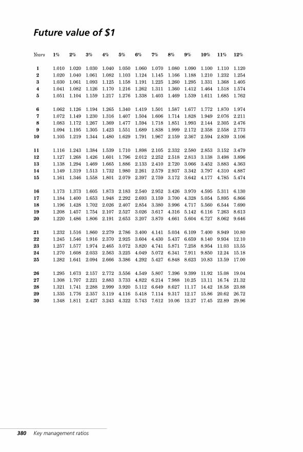
380 Key management ratios
Future value of $1
Years 1% 2% 3% 4% 5% 6% 7% 8% 9% 10% 11% 12%
1 1.010 1.020 1.030 1.040 1.050 1.060 1.070 1.080 1.090 1.100 1.110 1.1202 1.020 1.040 1.061 1.082 1.103 1.124 1.145 1.166 1.188 1.210 1.232 1.2543 1.030 1.061 1.093 1.125 1.158 1.191 1.225 1.260 1.295 1.331 1.368 1.4054 1.041 1.082 1.126 1.170 1.216 1.262 1.311 1.360 1.412 1.464 1.518 1.5745 1.051 1.104 1.159 1.217 1.276 1.338 1.403 1.469 1.539 1.611 1.685 1.762
6 1.062 1.126 1.194 1.265 1.340 1.419 1.501 1.587 1.677 1.772 1.870 1.9747 1.072 1.149 1.230 1.316 1.407 1.504 1.606 1.714 1.828 1.949 2.076 2.2118 1.083 1.172 1.267 1.369 1.477 1.594 1.718 1.851 1.993 2.144 2.305 2.4769 1.094 1.195 1.305 1.423 1.551 1.689 1.838 1.999 2.172 2.358 2.558 2.773
10 1.105 1.219 1.344 1.480 1.629 1.791 1.967 2.159 2.367 2.594 2.839 3.106
11 1.116 1.243 1.384 1.539 1.710 1.898 2.105 2.332 2.580 2.853 3.152 3.47912 1.127 1.268 1.426 1.601 1.796 2.012 2.252 2.518 2.813 3.138 3.498 3.89613 1.138 1.294 1.469 1.665 1.886 2.133 2.410 2.720 3.066 3.452 3.883 4.36314 1.149 1.319 1.513 1.732 1.980 2.261 2.579 2.937 3.342 3.797 4.310 4.88715 1.161 1.346 1.558 1.801 2.079 2.397 2.759 3.172 3.642 4.177 4.785 5.474
16 1.173 1.373 1.605 1.873 2.183 2.540 2.952 3.426 3.970 4.595 5.311 6.13017 1.184 1.400 1.653 1.948 2.292 2.693 3.159 3.700 4.328 5.054 5.895 6.86618 1.196 1.428 1.702 2.026 2.407 2.854 3.380 3.996 4.717 5.560 6.544 7.69019 1.208 1.457 1.754 2.107 2.527 3.026 3.617 4.316 5.142 6.116 7.263 8.61320 1.220 1.486 1.806 2.191 2.653 3.207 3.870 4.661 5.604 6.727 8.062 9.646
21 1.232 1.516 1.860 2.279 2.786 3.400 4.141 5.034 6.109 7.400 8.949 10.8022 1.245 1.546 1.916 2.370 2.925 3.604 4.430 5.437 6.659 8.140 9.934 12.1023 1.257 1.577 1.974 2.465 3.072 3.820 4.741 5.871 7.258 8.954 11.03 13.5524 1.270 1.608 2.033 2.563 3.225 4.049 5.072 6.341 7.911 9.850 12.24 15.1825 1.282 1.641 2.094 2.666 3.386 4.292 5.427 6.848 8.623 10.83 13.59 17.00
26 1.295 1.673 2.157 2.772 3.556 4.549 5.807 7.396 9.399 11.92 15.08 19.0427 1.308 1.707 2.221 2.883 3.733 4.822 6.214 7.988 10.25 13.11 16.74 21.3228 1.321 1.741 2.288 2.999 3.920 5.112 6.649 8.627 11.17 14.42 18.58 23.8829 1.335 1.776 2.357 3.119 4.116 5.418 7.114 9.317 12.17 15.86 20.62 26.7230 1.348 1.811 2.427 3.243 4.322 5.743 7.612 10.06 13.27 17.45 22.89 29.96
WKMR_Z04.QXD 11/24/05 12:51 PM Page 380
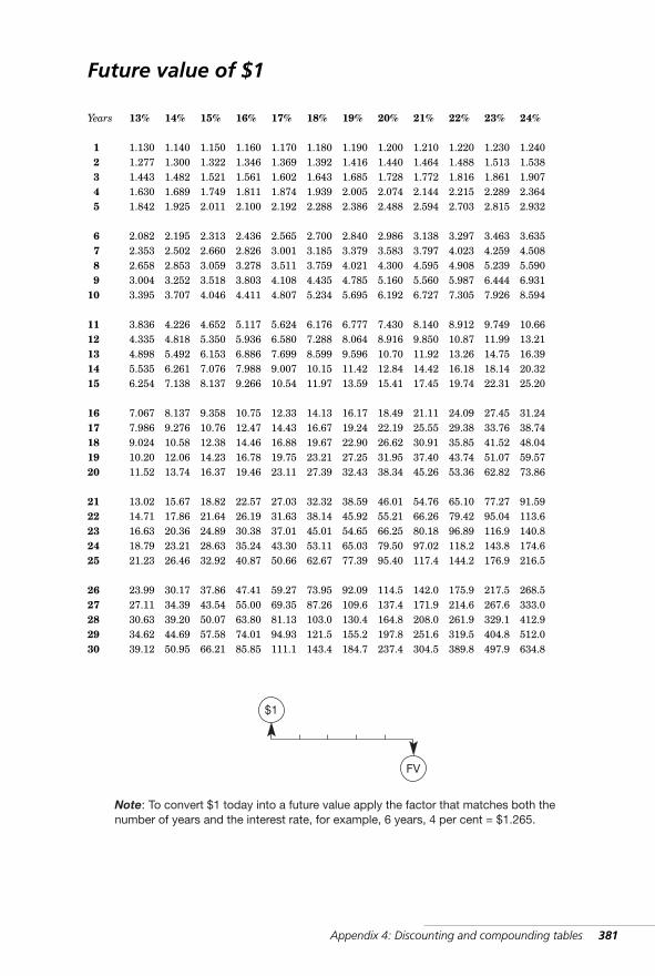
Appendix 4: Discounting and compounding tables 381
Future value of $1
Years 13% 14% 15% 16% 17% 18% 19% 20% 21% 22% 23% 24%
1 1.130 1.140 1.150 1.160 1.170 1.180 1.190 1.200 1.210 1.220 1.230 1.2402 1.277 1.300 1.322 1.346 1.369 1.392 1.416 1.440 1.464 1.488 1.513 1.5383 1.443 1.482 1.521 1.561 1.602 1.643 1.685 1.728 1.772 1.816 1.861 1.9074 1.630 1.689 1.749 1.811 1.874 1.939 2.005 2.074 2.144 2.215 2.289 2.3645 1.842 1.925 2.011 2.100 2.192 2.288 2.386 2.488 2.594 2.703 2.815 2.932
6 2.082 2.195 2.313 2.436 2.565 2.700 2.840 2.986 3.138 3.297 3.463 3.6357 2.353 2.502 2.660 2.826 3.001 3.185 3.379 3.583 3.797 4.023 4.259 4.5088 2.658 2.853 3.059 3.278 3.511 3.759 4.021 4.300 4.595 4.908 5.239 5.5909 3.004 3.252 3.518 3.803 4.108 4.435 4.785 5.160 5.560 5.987 6.444 6.931
10 3.395 3.707 4.046 4.411 4.807 5.234 5.695 6.192 6.727 7.305 7.926 8.594
11 3.836 4.226 4.652 5.117 5.624 6.176 6.777 7.430 8.140 8.912 9.749 10.6612 4.335 4.818 5.350 5.936 6.580 7.288 8.064 8.916 9.850 10.87 11.99 13.2113 4.898 5.492 6.153 6.886 7.699 8.599 9.596 10.70 11.92 13.26 14.75 16.3914 5.535 6.261 7.076 7.988 9.007 10.15 11.42 12.84 14.42 16.18 18.14 20.3215 6.254 7.138 8.137 9.266 10.54 11.97 13.59 15.41 17.45 19.74 22.31 25.20
16 7.067 8.137 9.358 10.75 12.33 14.13 16.17 18.49 21.11 24.09 27.45 31.2417 7.986 9.276 10.76 12.47 14.43 16.67 19.24 22.19 25.55 29.38 33.76 38.7418 9.024 10.58 12.38 14.46 16.88 19.67 22.90 26.62 30.91 35.85 41.52 48.0419 10.20 12.06 14.23 16.78 19.75 23.21 27.25 31.95 37.40 43.74 51.07 59.5720 11.52 13.74 16.37 19.46 23.11 27.39 32.43 38.34 45.26 53.36 62.82 73.86
21 13.02 15.67 18.82 22.57 27.03 32.32 38.59 46.01 54.76 65.10 77.27 91.5922 14.71 17.86 21.64 26.19 31.63 38.14 45.92 55.21 66.26 79.42 95.04 113.623 16.63 20.36 24.89 30.38 37.01 45.01 54.65 66.25 80.18 96.89 116.9 140.824 18.79 23.21 28.63 35.24 43.30 53.11 65.03 79.50 97.02 118.2 143.8 174.625 21.23 26.46 32.92 40.87 50.66 62.67 77.39 95.40 117.4 144.2 176.9 216.5
26 23.99 30.17 37.86 47.41 59.27 73.95 92.09 114.5 142.0 175.9 217.5 268.527 27.11 34.39 43.54 55.00 69.35 87.26 109.6 137.4 171.9 214.6 267.6 333.028 30.63 39.20 50.07 63.80 81.13 103.0 130.4 164.8 208.0 261.9 329.1 412.929 34.62 44.69 57.58 74.01 94.93 121.5 155.2 197.8 251.6 319.5 404.8 512.030 39.12 50.95 66.21 85.85 111.1 143.4 184.7 237.4 304.5 389.8 497.9 634.8
FV
$1
Note: To convert $1 today into a future value apply the factor that matches both thenumber of years and the interest rate, for example, 6 years, 4 per cent = $1.265.
WKMR_Z04.QXD 11/24/05 12:51 PM Page 381
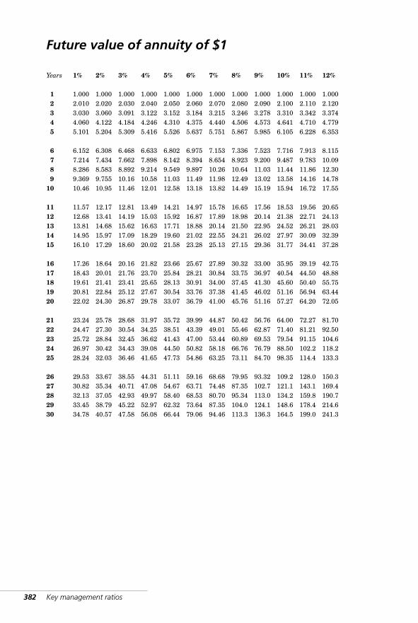
382 Key management ratios
Future value of annuity of $1
Years 1% 2% 3% 4% 5% 6% 7% 8% 9% 10% 11% 12%
1 1.000 1.000 1.000 1.000 1.000 1.000 1.000 1.000 1.000 1.000 1.000 1.0002 2.010 2.020 2.030 2.040 2.050 2.060 2.070 2.080 2.090 2.100 2.110 2.1203 3.030 3.060 3.091 3.122 3.152 3.184 3.215 3.246 3.278 3.310 3.342 3.3744 4.060 4.122 4.184 4.246 4.310 4.375 4.440 4.506 4.573 4.641 4.710 4.7795 5.101 5.204 5.309 5.416 5.526 5.637 5.751 5.867 5.985 6.105 6.228 6.353
6 6.152 6.308 6.468 6.633 6.802 6.975 7.153 7.336 7.523 7.716 7.913 8.1157 7.214 7.434 7.662 7.898 8.142 8.394 8.654 8.923 9.200 9.487 9.783 10.098 8.286 8.583 8.892 9.214 9.549 9.897 10.26 10.64 11.03 11.44 11.86 12.309 9.369 9.755 10.16 10.58 11.03 11.49 11.98 12.49 13.02 13.58 14.16 14.78
10 10.46 10.95 11.46 12.01 12.58 13.18 13.82 14.49 15.19 15.94 16.72 17.55
11 11.57 12.17 12.81 13.49 14.21 14.97 15.78 16.65 17.56 18.53 19.56 20.6512 12.68 13.41 14.19 15.03 15.92 16.87 17.89 18.98 20.14 21.38 22.71 24.1313 13.81 14.68 15.62 16.63 17.71 18.88 20.14 21.50 22.95 24.52 26.21 28.0314 14.95 15.97 17.09 18.29 19.60 21.02 22.55 24.21 26.02 27.97 30.09 32.3915 16.10 17.29 18.60 20.02 21.58 23.28 25.13 27.15 29.36 31.77 34.41 37.28
16 17.26 18.64 20.16 21.82 23.66 25.67 27.89 30.32 33.00 35.95 39.19 42.7517 18.43 20.01 21.76 23.70 25.84 28.21 30.84 33.75 36.97 40.54 44.50 48.8818 19.61 21.41 23.41 25.65 28.13 30.91 34.00 37.45 41.30 45.60 50.40 55.7519 20.81 22.84 25.12 27.67 30.54 33.76 37.38 41.45 46.02 51.16 56.94 63.4420 22.02 24.30 26.87 29.78 33.07 36.79 41.00 45.76 51.16 57.27 64.20 72.05
21 23.24 25.78 28.68 31.97 35.72 39.99 44.87 50.42 56.76 64.00 72.27 81.7022 24.47 27.30 30.54 34.25 38.51 43.39 49.01 55.46 62.87 71.40 81.21 92.5023 25.72 28.84 32.45 36.62 41.43 47.00 53.44 60.89 69.53 79.54 91.15 104.624 26.97 30.42 34.43 39.08 44.50 50.82 58.18 66.76 76.79 88.50 102.2 118.225 28.24 32.03 36.46 41.65 47.73 54.86 63.25 73.11 84.70 98.35 114.4 133.3
26 29.53 33.67 38.55 44.31 51.11 59.16 68.68 79.95 93.32 109.2 128.0 150.327 30.82 35.34 40.71 47.08 54.67 63.71 74.48 87.35 102.7 121.1 143.1 169.428 32.13 37.05 42.93 49.97 58.40 68.53 80.70 95.34 113.0 134.2 159.8 190.729 33.45 38.79 45.22 52.97 62.32 73.64 87.35 104.0 124.1 148.6 178.4 214.630 34.78 40.57 47.58 56.08 66.44 79.06 94.46 113.3 136.3 164.5 199.0 241.3
WKMR_Z04.QXD 11/24/05 12:51 PM Page 382
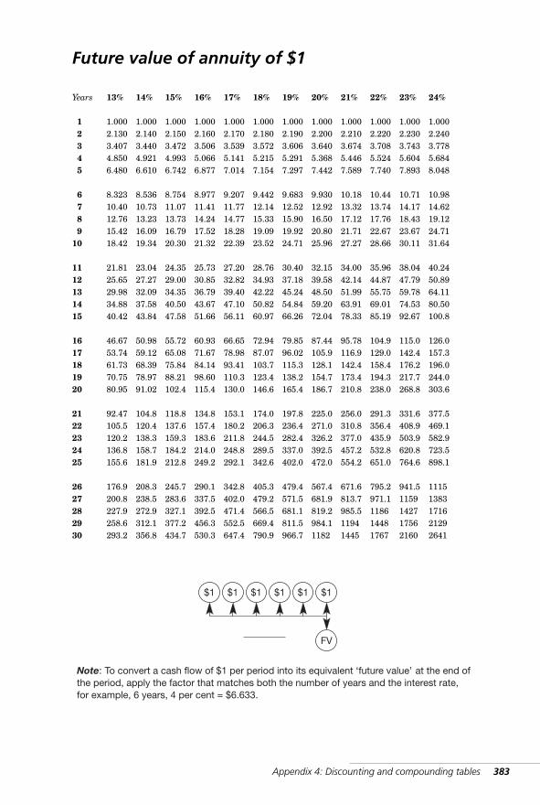
Future value of annuity of $1
Years 13% 14% 15% 16% 17% 18% 19% 20% 21% 22% 23% 24%
1 1.000 1.000 1.000 1.000 1.000 1.000 1.000 1.000 1.000 1.000 1.000 1.0002 2.130 2.140 2.150 2.160 2.170 2.180 2.190 2.200 2.210 2.220 2.230 2.2403 3.407 3.440 3.472 3.506 3.539 3.572 3.606 3.640 3.674 3.708 3.743 3.7784 4.850 4.921 4.993 5.066 5.141 5.215 5.291 5.368 5.446 5.524 5.604 5.6845 6.480 6.610 6.742 6.877 7.014 7.154 7.297 7.442 7.589 7.740 7.893 8.048
6 8.323 8.536 8.754 8.977 9.207 9.442 9.683 9.930 10.18 10.44 10.71 10.987 10.40 10.73 11.07 11.41 11.77 12.14 12.52 12.92 13.32 13.74 14.17 14.628 12.76 13.23 13.73 14.24 14.77 15.33 15.90 16.50 17.12 17.76 18.43 19.129 15.42 16.09 16.79 17.52 18.28 19.09 19.92 20.80 21.71 22.67 23.67 24.71
10 18.42 19.34 20.30 21.32 22.39 23.52 24.71 25.96 27.27 28.66 30.11 31.64
11 21.81 23.04 24.35 25.73 27.20 28.76 30.40 32.15 34.00 35.96 38.04 40.2412 25.65 27.27 29.00 30.85 32.82 34.93 37.18 39.58 42.14 44.87 47.79 50.8913 29.98 32.09 34.35 36.79 39.40 42.22 45.24 48.50 51.99 55.75 59.78 64.1114 34.88 37.58 40.50 43.67 47.10 50.82 54.84 59.20 63.91 69.01 74.53 80.5015 40.42 43.84 47.58 51.66 56.11 60.97 66.26 72.04 78.33 85.19 92.67 100.8
16 46.67 50.98 55.72 60.93 66.65 72.94 79.85 87.44 95.78 104.9 115.0 126.017 53.74 59.12 65.08 71.67 78.98 87.07 96.02 105.9 116.9 129.0 142.4 157.318 61.73 68.39 75.84 84.14 93.41 103.7 115.3 128.1 142.4 158.4 176.2 196.019 70.75 78.97 88.21 98.60 110.3 123.4 138.2 154.7 173.4 194.3 217.7 244.020 80.95 91.02 102.4 115.4 130.0 146.6 165.4 186.7 210.8 238.0 268.8 303.6
21 92.47 104.8 118.8 134.8 153.1 174.0 197.8 225.0 256.0 291.3 331.6 377.522 105.5 120.4 137.6 157.4 180.2 206.3 236.4 271.0 310.8 356.4 408.9 469.123 120.2 138.3 159.3 183.6 211.8 244.5 282.4 326.2 377.0 435.9 503.9 582.924 136.8 158.7 184.2 214.0 248.8 289.5 337.0 392.5 457.2 532.8 620.8 723.525 155.6 181.9 212.8 249.2 292.1 342.6 402.0 472.0 554.2 651.0 764.6 898.1
26 176.9 208.3 245.7 290.1 342.8 405.3 479.4 567.4 671.6 795.2 941.5 111527 200.8 238.5 283.6 337.5 402.0 479.2 571.5 681.9 813.7 971.1 1159 138328 227.9 272.9 327.1 392.5 471.4 566.5 681.1 819.2 985.5 1186 1427 171629 258.6 312.1 377.2 456.3 552.5 669.4 811.5 984.1 1194 1448 1756 212930 293.2 356.8 434.7 530.3 647.4 790.9 966.7 1182 1445 1767 2160 2641
Appendix 4: Discounting and compounding tables 383
FV
$1 $1 $1 $1 $1 $1
Note: To convert a cash flow of $1 per period into its equivalent ‘future value’ at the end ofthe period, apply the factor that matches both the number of years and the interest rate,for example, 6 years, 4 per cent = $6.633.
WKMR_Z04.QXD 11/24/05 12:51 PM Page 383
384 Key management ratios
All items in italics are defined elsewhere in the glossary
Acid test See quick ratio.Activity ratios These measure the relationship between key assets and sales.
They express how well assets are being utilized. For instance, ‘accounts receiv-able days’ (see debtor days) shows how long cash is tied up in accountsreceivable; likewise inventory days. We use the sales to fixed assets ratio to givea measure of the output being generated by major fixed assets. The term ‘assetutilization ratios’ is also used in this context.
Amortization of loan The repayment of a loan by equal periodic payments thatinclude both interest on outstanding balance plus some repayment of principal.
Annuity A series of equal payments made at equal intervals of time. Many finan-cial calculations can be treated by the annuity formulae, for examplerepayment of a term loan, straight line depreciation charges, and so on.
Arbitrage The operation of buying and selling a security simultaneously in twodifferent markets to take advantage of inconsistencies in pricing.
Asset backing Also known as ‘asset value per share’, it is calculated by dividingtotal ordinary funds in the balance sheet by the number of issued ordinaryshares.
Asset utilization ratios See activity ratios.Asset value per share See asset backing.Authorized share capital The maximum value of share capital that can be
issued. It is specified in the company Articles and can be increased only by per-mission of the shareholders.
Average collection period As debtor days.Average interest rate paid The apparent rate of interest paid on loans, calcu-
lated by expressing the interest charge in the profit and loss account as apercentage of loan funds in the balance sheet. It must be kept in mind that loansat the balance sheet date may not be a true reflection of the average over the year.
Bear Term for an investor who anticipates a falling market in financial securi-ties. This investor may sell securities not owned in order to profit from theexpected drop in price. See also bull.
Beta value A measure of the risk in a share that cannot be eliminated by diver-sification. High risk brings the need for a high return. Therefore the beta valueis used by analysts to derive an appropriate share value.
Blue chip A first-class commercial security.Bond US term for medium- to long-term loan. Legally it is the certificate that gives
the holder the right to periodic interest payments and repayment of principal.Bonus issue New equity shares issued from reserves and given free to company
shareholders in proportion to their existing share holdings.Book value per share The value of a share based on the balance sheet values.
See also asset backing.
Glossary
WKMR_Z05.QXD 11/24/05 12:51 PM Page 384
Glossary 385
Borrowing ratio Long-term plus short-term loans expressed as a percentage ofordinary funds plus preference shares less intangibles.
Break-even analysis A form of analysis that relates activity to totals of revenueand costs based on the classification of costs into fixed and variable types.
Break-even point The level of activity at which the fixed costs of an operationare just covered by the contribution from sales. At this point neither a profitnor a loss ensues.
Bull An investor who anticipates a rise in the price level of financial securities.This investor may purchase securities with the intention of resale before thetime for settlement is due. See also bear.
Bullet A single payment of the total amount of a loan at the end of the period (asopposed to periodic payments during its life).
Capital asset pricing model (CAPM) A model that links risk and return forall types of security. Applied to the valuation of equity shares, it uses the riskcoefficient (beta value) of the share to calculate the required risk premium.This risk premium is added to the risk-free rate (rate on gilts) to give theappropriate yield for the share.
Call The amount demanded from shareholders from the balance outstanding onnon-paid-up shares.
Call option An option to purchase. See also option.Capital employed The total of the long-term funds in the balance sheet. It
includes shareholders’ funds, long-term loans, preference shares, minorityinterests and miscellaneous long-term funds. It can also be expressed as totalassets less current liabilities.
Capital market The financial market for long-term securities.Capital project appraisal Evaluation of expenditure on capital assets to estab-
lish its rate of return with a view to deciding on whether or not to make theinvestment.
Capital reserves Shareholders’ funds that have originated from sources otherthan trading or the nominal value of new issues.
Capital structure The mix of financing in a company. It usually refers to theproportions of debt and equity in the balance sheet.
Cash cycle A model of working capital cash flow that identifies the timerequired for cash paid out for raw materials and expenses to come back in fromaccounts receivable.
Cash flow, incremental The extra cash in-flow or out-flow that comes fromselecting one alternative over another in capital project appraisal.
Cash flow per share Profit after interest, tax, minority and preference divi-dends plus depreciation divided by the number of shares.
Caveat emptor ‘Let the buyer beware’ – an expression that emphasizes the dutyof a party to a contract to ensure that his interests are protected.
Certificate of deposit (CD) A short-term negotiable certificate issued by abank as evidence of a deposit that is repayable on a fixed date. It is a highlyliquid bearer instrument.
Collateral A physical or financial asset used as security for a loan.Commercial paper Loan notes issued by high-credit corporations to raise
short-term funds direct from the money markets rather than from a lendinginstitution.
Common size financial statements Statements that have been standardizedby having each component expressed as a percentage of sales or total assets.
WKMR_Z05.QXD 11/24/05 12:51 PM Page 385
386 Key management ratios
Compensating balance The minimum amount by which a company must stayin credit on a deposit account under the terms of a loan.
Consols UK Government stock secured on the Consolidated Fund. Theyare effectively non-redeemable loans to the government with a low nominalinterest rate.
Constant growth model A valuation model, derived by Professor Gordon, thatcalculates a share value from its dividend flow to infinity under assumptions ofconstant growth.
Contingent liability A potential liability that may not arise but which must bementioned in the notes to the published accounts of a company.
Conversion ratio The number of shares the holder of a convertible securityreceives for each bond on conversion.
Convertible loan A loan that gives the lender the option to convert into sharesat a fixed price for a period of time.
Cost of capital The weighted average cost of funds to a company, based on themix of equity and loan capital and their respective costs. A distinction is usu-ally drawn between the average cost of all funds in an existing balance sheetand the marginal cost of raising new funds.
Covenant, restrictive A clause in a loan agreement to restrict the freedom ofthe borrower to act in a way that would weaken the position of the lender, suchas increasing the amount of the dividend.
Credit period The number of days’ sales represented by the accounts receiv-able. It corresponds with the term debtor days.
Current assets The sum of inventories, accounts receivable, cash and cashequivalents and miscellaneous short-term assets.
Current liabilities The sum of accounts payable, short-term loans and miscella-neous accruals all due for repayment within one year.
Debenture A legal document that acknowledges a loan. In the US, the termrefers to an unsecured loan. In the UK it may be secured by a fixed or floatingcharge on the assets.
Debtor days, or, accounts receivable days The figure for trade debtors in thebalance sheet is divided by the average sales per day to express the averagenumber of days’ credit taken by customers.
Debt to equity ratio The principal measure of the mix of funds in a company’sbalance sheet. It can be expressed in a number of different ways. The mostcommon way is to calculate the percentage that total interest bearing debtbears to ordinary plus preference shareholders’ funds.
Debt to total assets ratio One of the debt to equity measures. Long-term loansplus current liabilities are expressed as a percentage of total assets.
Deferred tax A taxation amount that has been charged to the profit and lossaccount but which has not been paid over to the authorities and is not currentlypayable. Timing differences between accounting and taxation computations oftaxable profit on account of depreciation and so on are the root cause.
Departmental ratios The effectiveness of the major departments can beassessed by using an approach similar to that for the total operation, as illus-trated in chapter 7. For each department, costs and assets classified underselected headings are related to sales, cost of sales or standard hours of workproduced as appropriate. Suggested ratios for Marketing and Production areshown below:
WKMR_Z05.QXD 11/24/05 12:51 PM Page 386
■ Marketing: cost to sales ratiossalaries and commissiontravel expensesadvertising costssales office costs
■ Marketing: assets to sales ratiosfixed assets: officefixed assets: cars/equipmentfinished goodsaccounts receivable
■ Production: cost to cost of sales ratiosdirect materialdirect laborovertimeindirect labormaintenanceproduction planningsupervision and so on
■ Production: assets to cost of sales ratiosfixed assets: factory premisesfixed assets: plantfixed assets: vehiclesraw materialwork in progress.
Dilution The reduction in the earnings per share value due to an increase in thenumber of shares issued or contracted to be issued in the future.
Discounted cash flow (DCF) A method of appraisal for investment projects.The total incremental stream of cash from a project is tested to assess thereturn it delivers to the investor. If the return exceeds the required, or, hurdlerate, the project is recommended on financial terms and vice versa. Twoapproaches can be used in the assessment: see net present value (NPV) andinternal rate of return (IRR).
Discounting A technique used to calculate the present value of a cash flowoccurring in some future time period. It is used in connection with the sale forimmediate cash of a future debt and, more extensively, in translating futurecash flow from an investment into present values.
Dividend cover Expresses the number of times that dividends to the ordinaryshareholders are covered by earnings. See also payout ratio.
Dividend per share (DPS) The actual dividend paid on each ordinary share. Itcan be calculated from the accounts by dividing the total ordinary dividend bythe number of ordinary shares.
Dividend yield Actual dividend per share expressed as a percentage of the cur-rent share price. In the UK, imputed tax is added to dividends paid and thecalculation gives gross dividend yield.
Earnings per share (EPS) The profit earned for the ordinary shareholders asshown in the profit and loss account is divided by the number of issued ordi-nary shares to give earnings per share. (To be strictly orthodox, the weightedaverage number of shares should be used.)
Earnings yield Earnings per share expressed as a percentage of the currentshare price. In the UK, imputed tax is added to earnings to give gross yield.
Glossary 387
WKMR_Z05.QXD 11/24/05 12:51 PM Page 387
388 Key management ratios
EBITDA Earnings before interest, tax, depreciation and amortization (seeappendix 1 for explanation).
Employee ratios To measure the productivity of labor, three major variables –sales, profits and assets – are related back to the number of employees andtheir remuneration. The principal ratios used are:■ remuneration to employee■ sales to employee■ sales to remuneration■ profit to employee■ profit to remuneration■ fixed assets to employee■ working capital to employee.
Equity gearing Common funds plus preference shares expressed as percentageof long-term loan plus current liabilities.
Eurodollar Deposits denominated in US dollars in a bank outside the US ownedby a non-resident of the US.
Extraordinary item A significant transaction outside the normal activities ofthe business and likely to be non-recurring. An example would be the sale ofthe corporate head office at a large profit. There is a strong argument that sucha transaction should not be allowed to distort the trading results and that itshould be isolated from the reported earnings. However, the contrary argumentthat all such gains and losses should be included in the profit and loss accountnow prevails.
Factoring A method of raising funds by the selling of trade debtors.Fixed assets Land and buildings, plant and equipment and other long-term
physical assets on which the operations of the company depend.Fixed cost A type of cost where the total expenditure does not vary with the
level of activity or output.Floating rate note (FRN) Loan on which the interest rate varies with prevail-
ing short-term market rates.Forward cover The purchase or sale of foreign currency for delivery at a fixed
future time. It is used to cover against the risk of an adverse exchange ratemovement.
Forward exchange rate A rate fixed to govern the exchange of currencies at afixed future date.
Free borrowing percentage The percentage of non-equity funds that is madeup of ‘free’ debt, that is accounts payable, accruals and deferred tax.
Futures contract A contract in an organized exchange to trade in a fixed quan-tity of a security at a fixed price at a future date.
Gearing A relationship between different types of funds in a company, such asloans and equity. The higher the amount of loan funds the higher the amountof fixed interest charge in the profit and loss account. Where interest chargesare high, a small change in operating profit will have a much increased resultin return to the equity for shareholders.
Gilts The term ‘gilt-edged’ refers to government longer term borrowing instru-ments. They are described as ‘short’ where the maturity is up to five years,‘medium’ for periods of five to 15 years and ‘long’ for over 15 years to infinity.
Hedging A technique for reducing the risk of an exposed position by taking acompensating position in another security.
WKMR_Z05.QXD 11/24/05 12:51 PM Page 388
Hurdle rate The rate of return decided on by a company as the minimumacceptable for capital investment. It will be governed by the firms’ cost of capi-tal and it may allow for different levels of risk.
Intangible assets Long-term non-physical assets in the balance sheet such asgoodwill and brand values.
Interest cover A liquidity ratio that expresses the number of times the interestcharged in the profit and loss account is covered by profit before interest and tax.
Internal rate of return (IRR) The rate of discount that brings the presentvalue of all the cash flows associated with a capital investment to zero. It meas-ures the effective yield on the investment. If this yield is greater thanthe ‘hurdle rate’ the investment is deemed to be financially desirable andvice versa.
Inventory days The inventory value in the balance sheet is expressed in termsof days. The divisor is usually the average daily cost of sales. Separate calcula-tions are made for raw materials, work in progress and finished goods.
Investments Investments in subsidiary and associated companies and otherlong-term financial assets.
Junk bonds High-interest-bearing bonds with little security of assets issued bya company with good cash flow.
LIBOR London InterBank Offered Rate – the rate at which major banks in theshort-term money market lend to each other. It is a benchmark for many inter-national loans and floating-rate issues to corporations.
Lease – finance A lease under which the lessee assumes all the risks andrewards of ownership. It extends over the estimated economic life of the assetsand cannot easily be canceled. Under current accounting rules, such a lease istreated as a loan.
Leverage See gearing.Leveraged buy-out The acquisition of a firm by using large amounts of debt.Liquidity The ability to provide cash to meet day-to-day needs as they arise.Long-term loans (LTL) Bank and other loans of more than one year.Market capitalization The notional total market value of a company calculated
from the latest quoted market price of the share multiplied by the number ofshares. The quoted price may not give an accurate value for the total shares, itmay refer to only one small block of shares.
Market to book ratio The relationship between the balance sheet value ofthe ordinary shares and their market value. The expression ‘price to book’ isalso used.
Market value weights In cost of capital calculations, the weighted cost can bederived using either the book value or market value weights to determine theoverall weighted cost.
Matching principle A rule that a firm should match short-term uses of fundswith short-term sources and long-term uses with long-term sources.
Minority interests The book value of shares in a subsidiary that are owned bymembers who are not shareholders of the parent company.
Miscellaneous current assets Sundry receivables and pre-payments due forrealization within one year.
Miscellaneous long-term funds A composite entry in the balance sheet thatmay include deferred tax, unamortized government grants, provision for pen-sions and so on.
Money market A term applied to the trading in short-term financial instru-ments in London.
Glossary 389
WKMR_Z05.QXD 11/24/05 12:51 PM Page 389
390 Key management ratios
Mutually exclusive projects In an investment appraisal exercise these areprojects that compete with one another so that the acceptance of one means theexclusion of the others.
Net working capital See working capital.Net worth (NW) The sum of common ordinary shares plus all reserves plus
preference shares less intangible assets.Net present value (NPV) A positive or negative value arrived at by discounting
the cash flow from a capital project by the desired rate of return. If the value ispositive, it means that the project is financially desirable and vice versa.
NOPAT Net operating profit after tax (see chapter 17 for explanation).Off-balance sheet A term that refers to borrowing that does not appear on the
balance sheet. Sometimes achieved by a finance lease that gives the lessee allthe risks and rewards, but not the legal status, of ownership.
Opportunity cost The alternative advantage foregone as a result of the commit-ment of resources to one particular end.
Optimal capital structure The point at which the cost of capital to a companyis reduced to the minimum by the best mix of debt and equity.
Option A financial instrument that gives the holder the right, but not the obliga-tion, to purchase or sell a specified asset at a specified price on or before a setdate. See put option; call option.
Over the counter (OTC) Refers to the market where shares and financialinstruments are traded outside the formal exchanges.
Overtrading A company is in an overtrading situation when there is not suffi-cient liquidity to meet comfortably the day-to-day cash needs of the existinglevel of business. There is constant danger of bankruptcy, even though the com-pany may be trading profitably. Such a situation can come about because ofpast trading losses, excessive expansion and so on, but can be cured by theinjection of long-term funds or, maybe, the sale of fixed assets.
Owners’ funds (OF) The sum of the issued shares, capital reserves and revenuereserves. The total represents the assets remaining to the shareholders after allprior claims have been satisfied.
Paid borrowing percentage The percentage of non-equity funds consisting ofinterest-bearing debt.
Par value A notional value assigned to a share largely for accounting purposes.Payback period A term used in investment appraisal. It refers to the time
required for the non-discounted cash in-flow to accumulate to the initial cashout-flow in the investment.
Payout ratio The percentage of earnings available for distribution that is paidout in dividends. This ratio is the reciprocal of dividend cover.
Preference capital Shares that have preferential rights over common shares.These rights normally relate to distribution of dividends and repayment ofcapital. The shares usually carry a fixed dividend but also carry very littlevoting power.
Preferred creditors Creditors who, in an insolvency, have a statutory right tobe paid in full before any other claims. Employees who have pay due to themwould normally be in this category.
Present value (PV) A sum calculated by discounting the stream of future cashflow from a project using an interest rate equal to the desired rate of return. Itdiffers from net present value in that the amount of the investment is notincluded in the cash flows.
WKMR_Z05.QXD 11/24/05 12:51 PM Page 390
Price to earnings multiple (PE) The value derived by dividing the currentshare price by the earnings per share. Latest reported earnings or prospectiveearnings for the coming year may be used in the calculation.
Prime rate The rate at which banks lend to corporations with the highest creditratings.
Profit after tax (PAT) Profit available for the shareholders after interest andtax has been deducted.
Profit before interest and tax (PBIT) Operating profit plus other income.Profit before interest, tax and depreciation (PBITD) This value corre-
sponds very closely to cash flow from trading.Profit before tax (PBT) Operating profit plus other income less total interest
charged.Profitability index A measure for assessing the relative merit of an investment
by expressing the present value of the future cash flows as a percentage of theinvestment amount.
Pro forma statements Projected financial statements.Proxy vote Vote cast by an authorized person on behalf of another.Put option An option to sell. See also option. Quick ratio (acid test) A short-term liquidity ratio calculated by dividing cur-
rent assets less inventories by current liabilities.Repurchase agreement (REPO) A technique for providing short-term cash to
a borrower who agrees to sell a security at one price and buy it back at aslightly higher price in the future. The price difference is the effective interestpayment to the lender.
Retained earnings (RE) The final figure from the profit and loss account thatis transferred to reserves in the balance sheet.
Return on capital This is profit before tax but after interest as a percentage ofcapital employed.
Revenue reserves Increases in shareholders’ funds that have arisen fromretained profits and are available for distribution as dividends.
Rights issue A new issue of shares made by a company to its existing shareholdersat a price below the current market value.
Risk-free rate of interest The yield available on government gilts.Return on assets (ROA) Profit before interest and tax as percentage of total
assets. The corresponding term used in this book is return on total assets.Return on capital employed (ROCE) Capital employed includes all the long-
term funds in the balance sheet, that is shareholders’ funds plus long-termloan plus miscellaneous long-term funds. Profit before tax is often expressed asa percentage of this to give return on capital employed. However, as the denom-inator includes long-term loan, the corresponding interest on these loansshould be added back into the numerator.
Return on equity (ROE) A measure of the percentage return generated by acompany for the equity shareholders. It is calculated by expressing profit aftertax as a percentage of shareholders’ funds. (Where preference shares exist, theyshould first be deducted from shareholders’ funds and the preference dividendsalso be deducted from the profit figure.)
Return on invested capital (ROIC) See chapter 17 for explanation.Return on investment (ROI) A term that is very widely used in connection
with the performance of a company or project. It is calculated in many differentways. Usually a pre-tax profit figure is expressed as a percentage of either thelong-term funds or the total funds in the balance sheet.
Glossary 391
WKMR_Z05.QXD 11/24/05 12:51 PM Page 391
392 Key management ratios
Return on total assets (ROTA) Profit before interest and tax expressed as apercentage of total assets.
Sales and leaseback agreement A method of raising finance whereby a firmsells property to the funding agency and simultaneously signs a long-term leaseagreement. The company receives an immediate lump sum in exchange for aseries of lease payments in the future.
Sales to fixed assets (times) An activity and performance ratio, calculated bydividing the net fixed assets value in the balance sheet into the sales turnoverfigure.
Senior debt Debt that ranks ahead of junior, or, subordinated debt in the eventof a liquidation. See subordinated debt.
Sensitivity analysis Analysis of the change in the output values of an equationfrom small changes in input values. It is used to assess the risk in an invest-ment project.
Share premium The difference between a share’s nominal value and its sale price.Shareholders’ funds Issued ordinary shares plus reserves plus preference shares.Short-term loans (STL) The bank overdraft, current portion of long-term debt
and other interest-bearing liabilities due within one year.Spontaneous financing Short-term financing that automatically results from
the normal operations of the business. Creditors/accounts payable and certainaccruals are the main sources.
Subordinated debt Debt that ranks for repayment after senior debt.Subsidiaries A company is a subsidiary of another if the other owns more than
50 per cent of the equity or effectively controls the company by means of votingshares or composition of the board of directors.
Sundry accruals An entry in the current liabilities section of the balance sheetthat includes sundry accounts payable plus accrued dividends, interest, tax plusother accruals.
SWAP The exchange of debt and/or currency obligations between parties to theirmutual benefit. The benefit can arise from their differing needs for currencyand/or fixed/floating interest charges.
Tangible assets The total of all assets in the balance sheet less intangibles, suchas goodwill.
Tax rate The apparent rate of tax on profit found by expressing tax charged inthe accounts as a percentage of profit before tax.
Term loan Usually a medium-term loan (three to seven years) repaid infixed, periodic instalments that cover both interest and principal over the life ofthe loan.
Terminal value A notional cash in-flow attributed to a capital project to allowfor value remaining in the project at the final year of the assessment.
Total assets The sum of fixed assets plus intangibles plus investments plus cur-rent assets.
Treasury stock Ordinary or common shares that have been repurchased by thecompany.
Ultra vires ‘Beyond authorized powers’. An act is deemed to be ultra vires ifcarried out by an agent or director of a company in excess of their authority.The person who so acts may incur personal liability.
Underwriting Banks or other financial institutions guarantee to take up anissue of shares at a specific price in order to ensure the success of the issue.This process in called underwriting.
WKMR_Z05.QXD 11/24/05 12:51 PM Page 392

Variable costs A type of cost where the total expenditure varies in proportion toactivity or output.
Warrant Sometimes attached to loan stock as a sweetener at the time of issue,warrants give an option to the holder to purchase a stated amount of equitiesat a fixed price for a defined period.
Weighted average cost of capital (WACC) See cost of capital.Window dressing The alteration of financial statements at the time of publica-
tion to give an artificially improved appearance to the company situation. Forinstance the temporary sale of inventories to a bank with agreement to repur-chase could give an enhanced view of company liquidity.
Working capital The excess of current assets over current liabilities.Working capital days The length of the working capital cycle is often calcu-
lated as inventories plus accounts receivable less accounts payable days.Working capital to sales A liquidity ratio that is calculated by expressing
working capital as a percentage of sales.Z-growth factor A value that gives an indication of the self-funding growth rate
of a company. It is calculated by expressing retained earnings before extraordi-nary items as a percentage of opening owners’ funds. It is assumed for thiscalculation that all assets are linearly related to sales, likewise all items in theprofit and loss account. It also assumes that existing debt to equity ratios willbe maintained.
Zero coupon bond A bond that pays no interest but is issued at a discount onits face value. The redemption of the bond at par ensures the desired yield tothe purchaser.
Glossary 393
WKMR_Z05.QXD 11/24/05 12:51 PM Page 393
394 Index
absolute values, acquisition analysis312–15
accelerated capital allowances 345accounting policies 323, 327accounting standards 150–1accounting statements see financial
statements; integrity of accounting statements
accounts payable 100, 146, 264, 333accounts receivable 16–17, 86, 100,
90–1, 264, 331accounts receivable days 327, 363accruals, undervalued 332–3acid test ratios see quick ratiosacquisition analysis 291–3
earnings per share 298–309financial profiles 294–7first offers 298–309revised offers 310–11shareholder effects 302–9shareholder value added 312–19values, relative versus absolute
312–15acquisitions 202, 340–3administration costs 84–5, 212–3amortization 328–9, 351–2annuities tables 376–7, 380–1annuity approach, terminal values
calculations 352–3appropriation of profits 40–1
APS (assets per share) 304–9, 311assets
backing 158–9on balance sheets 14–15, 16–20current see current assetsfixed see fixed assetsintangible 18–19, 340long-term 32non-operating 274operating 264–5overvalued 331–2
recognition 329sales to total assets see salessector parameters 79per share (APS) 304–9, 311total see return on total assets; total
assetsturn 72–3, 185–6values 158–9
associated companies, sales to 326average returns to total equity market
280–1
backdating revenues 324background 2–7bad debt reserves 330balance sheets
assets see assetsfunction 12, 13horizontal format 55integrity 331–5layouts 54–7liabilities see liabilitiesprofit and loss accounts, relationship
with 50–2shareholder value added 264, 272structure 16–24terms 25–34vertical formats 54–7
bankruptcy 99, 120banks 128, 146beta values 280–1big bath 330–1bill and hold 325bogus sales 327bonus issues 348–9book values 21, 158–9break-even 218, 220–5
capitalemployed 28–9, 56–7
return on (ROCE) 52
Index
WKMR_Z06.QXD 24/11/05 1:36 pm Page 394
equity, cost of 278–9expenditure 106–7invested see invested capitalweighted average cost of 276–7, 314working see working capital
capital allowances, accelerated 345capital asset pricing model (CAPM)
280–1capital investment, future 261
see also project appraisalscapital leases 334capital reserves 23–4capitalization 156, 159, 329–30CAPM (capital asset pricing model)
280–1cash 16, 99
asset purchases, spent on 38availability, liquidity as indicator of
32closing reconciliations 144–5cycle 100–110importance 100opening reconciliations 144–5shareholder value added 264
cash flow cyclescapital expenditure 106–7cash 99company profiles 110–111current ratios 116–17dividends 106–7interest 106–7liquidity measures, long and short
analysis 110–111loan repayments 106–7new equity capital 108–9new long-term loans 108–9non-operating cash in-flows 108–9non-operating cash out-flows 106–7
cash flow statementsconstruction of 142function 12, 13, 139hidden movements 142indirect method 142integrity 335–8profit and loss accounts compared
139sources and uses of funds 140–3, 150
cash flowscontribution and 214cycles see cash flow cyclesdepreciation and 102–5, 268–70
financial reporting standards 150–1fixed outflows, debt servicing 132forecasts 268–9future, values determined by 262growth and 190long and short analysis 146–9negative 192net 268–9, 318from operations (CFFO) 337–8profits and 38, 102–3project appraisals 244, 246, 248–9revenue recognition manipulation
and 328statements see cash flow statements
CFFO (cash flows from operations)337–8
closing and opening cash reconciliations 144–5
collection periods 90–1, 94common stock, issued 21–2, 158company profiles 110–111compounding tables 374–81conditional sales 326consignment sales 325contra agreements 326contribution 214
calculation of 219cash flows and 214maximization 216, 236percentage of sales (CPS) 226–37product mix 234–5profits and 216–7total 216–8, 228–9fper unit (CPU) 216–7, 226, 230per unit of capacity 236, 238–9per unit of the limiting factor 236,
238corporate liquidity
cash flow cycles 96–111cash flows 137–51financial strength 125–6liquidity 113–23
corporate tax 366corporate value determinants
corporate valuation 155–74, 186–7financial leverage 175–87growth 189–203share values see shares: values
costsadministration 84–5, 212–3alternative costing approaches 215
Index 395
WKMR_Z06.QXD 24/11/05 1:37 pm Page 395
costs (continued) break-even see break-evencapitalized 329–30classification 212–3costing illustration 210–11debt 132equity 276factory overheads 84–5fixed 212–3, 216–7, 220–4labor 84–5, 212–3materials 84–5, 212–3operating 84–5, 328–31operating leverage 224–5ratios 84–5selling 84–5, 212–3timing adjustments 39total incurred 36total operating 84–5variable 212–3, 220–4weighted average cost of capital
(WACC) see weighted averagecost of capital
CPS (contribution percentage of sales)226–37
CPU (contribution per unit) 216–7,226, 230
creditors 56current assets 16–17, 110, 146, 148,
192, 264current assets to sales 194–201current liabilities 20–21, 28, 110,
128–9, 146, 148, 192, 264current ratios 116–17, 146, 148, 190,
294–7, 364
DCF (discounted cash flow) 256–7, 312debt 128–9, 132debt to equity ratios 128–34, 136, 148,
333–5, 342debt to total assets ratios 146, 190, 368debtor days 90–1, 94debtors 16decision-making see management
decision-makingdeferred tax 130, 330, 345, 350depreciation 38, 102–5, 268–70, 328–9,
335–6, 345, 351–2determinants of corporate value see
corporate value determinantsdiscount factors 246, 248–9, 276–85discounted cash flow (DCF) 256–7, 312
discounting tables 374–81distribution of profits 40–1dividends
cash flows and 106–7cover 164–7, 369per share (DPS) 162–3, 304–9, 311yield 168–70, 371
DPS see dividends: per share
earningscash flows from operations and
337–8growth 170retained earnings to sales 194–201
earnings after tax 40–1, 53, 160earnings before interest and tax
(EBIT) 40–1, 52–3, 64, 335–6earnings before interest, tax,
depreciation and amortization(EBITDA) 335–6, 351–2
earnings before tax 40–1, 53earnings per share (EPS) 160–2,
298–311earnings yield ratios 168–70, 182, 185,
186, 370EBIT see earnings before interest and
taxEBITDA (earnings before interest, tax,
depreciation and amortization)335–6, 351–2
economic value added (EVA) 261Enron 335EPS see earnings per shareequity
capital 108–9, 278–9costs 276debt to equity ratios see debt to
equity ratiosreturn on see return on equityvalues 274–5
EVA (economic value added) 261Example Co. plc 42–3excessive capitalization 329exchange rates 344extraordinary items 38
factory overheads 84–5fair values 340fictitious revenues 324, 326–7fictitious sales 326–7finance leases 345
396 Index
WKMR_Z06.QXD 24/11/05 1:37 pm Page 396
financial engineering 176financial leverage 126, 176–78, 180–1,
187financial profiles 294–7financial reporting standards 150–1financial statements 9–11
assets see assetsbalance sheets see balance sheetscash flow statements see cash flow
statementsintegrity see integrity of accounting
statementsliabilities see liabilitiesprofit and loss accounts see profit
and loss accountsfinancial strength 125–6finished goods 100fixed assets 18–19, 86, 110, 157
acquisition analysis 318depreciation and 329integrity 328revaluation of 346–7sales to 91shareholder value added 264, 266–8
fixed assets to sales 313–5fixed costs see costsforeign currencies 344funds
long-term 28, 32, 350non-equity 274, 314, 319owners 21–3, 110, 156–7self-funding 202–3sources 15–16, 140–3, 150uses 140–3, 143
future capital investment 261future values tables 378–81
gearing see leveragegeographical data 42, 44
charts 357–73debt 132–4dividend yield 168–9dividends cover 166–7growth 202–3market to book ratios 173–4price to earnings ratios 170–1return on equity 68–9return on total assets 76–7
glossary 382–91goods invoiced but not shipped 325goods shipped but not ordered 325
goodwill 340–3, 351–2grants 350gross margins 333gross profit to sales 332growth 189–90
acquisition analysis 294–7acquisitions, application to 202analysis 194–5earnings 170earnings per share 162equilibrium 196–204example 190–3long-term 352–3profits 162rates 194–201sales see salesself-funding 202–3share prices 162value and 283–5
hidden movements, cash flows 142historic values 261horizontal format balance sheets 55
impairment, goodwill 342income statements see profit and loss
accountsinstalment sales 325intangible assets 18–19, 340integrity of accounting statements
321–3balance sheets 326–35cash flow statements 335–8operating costs 328–31operating revenue enhancement
323–8interest
cash flows and 106–7cover 126–7, 294–7, 367
interest bearing debt 128internal rate of return (IRR) 254–5, 256inventories 16–17, 86, 157
accounts payable links 264integrity 328obsolescence reserves 330overvalued 331–2sales to 90–91
inventory days 92–3, 332, 362invested capital 264
return on (ROIC) 282–6investment funds 168
Index 397
WKMR_Z06.QXD 24/11/05 1:37 pm Page 397
398 Index
investments 18–19profiles 244–5project appraisal see project appraisalratios 241–57return on 61–2, 244
involuntary takeovers 99IRR (internal rate of return) 254–5, 256issued common stock 21–2, 158
labor costs 84–5, 212–3leases 334, 345legal claims, debt and 132leverage 134–5
acquisition analysis 294–7effects of 70financial see financial leverageoperating 224–5
liabilities 157on balance sheets 14–15, 20–4current see current liabilitieslong-term loans see long-term loansshort-term 28undervalued 332–3
limiting factor, contribution per unit of236, 238
liquidityacquisition analysis 294–7corporate see corporate liquiditycurrent ratios 116–17long and short analysis 110–111measures of 110–111quick ratios 118–19ratios 190short-term measures 115–21working capital as measure of 32working capital days 122–3working capital to sales ratios 120–1
loanslong-term see long-term loansrepayments 38, 106–7short-term 128–9
long and short analysis 110–111,146–9
long-term accounts receivable 327long-term assets 32long-term contracts, revenues 325long-term funds 28, 32, 350long-term growth approach, terminal
values calculations 352–3long-term loans 20–1, 108–9, 110,
128–9, 192
machine hours 238management decision-making
acquisition analysis 291–319cost, volume and price relationships
207–40integrity of accounting statements
321–38investment ratios 241–57shareholder value added 259–89
management performance 272–3manipulation of accounts see integrity
of accounting statementsmargins 72–7, 82–5, 184–5, 266,
313–5, 359market capitalization 156, 159market premiums 280–1market to book ratios 172–4, 182–7,
294–7, 300, 373market values 22, 160matching principle 148, 329materials 84–5, 100, 212–3minority interests 350MVA (market value added) 261
negative cash flows 192net cash flows 268–9, 318net fixed assets 18–19net operating profit after tax (NOPAT)
270, 318, 352–3net present values (NPV) 250, 252–3,
256net working capital 264, 266–8net worth 30–1nominal values 21, 158non-equity funds 274, 314, 319non-operating assets 274non-operating cash in-flows 108–9non-operating cash out-flows 106–7NOPAT see net operating profit after
taxnotes to accounts 323, 329NPV see net present values
offers, acquisition analysis 298–311opening and closing cash
reconciliations 144–5operating assets 264–5operating costs 84–5, 328–31operating leases 334operating leverage 224–5operating performance
WKMR_Z06.QXD 24/11/05 1:37 pm Page 398
drivers 81–94margins on sales 82–5measures of performance 48–57operating profit model 88–91return on capital employed 52return on equity see return on equityreturn on investment 61–2return on total assets see return on
total assetsstandards of 66–79
operating profits 40, 88–91, 270, 318operating revenue enhancement 323–8operations, cash flows from (CFFO)
337–8overdrafts 146overtrading 120overvalued assets 331–2owners’ funds 21–3, 110, 156–7ownership, risks and rights of 334
par values 158pay-back 243payments and receipts cash statements
142pay-out ratios 164–5PE ratios see price earnings ratiospensions 344performance
drivers 81–94managerial 272–4margins on sales 82–5measures of 49–57operating see operating performanceterms, multiplicity of 50
PPS (price per share) 303–9, 311preference shares 350premature revenues 324–5prepayments, overvalued 332present values (PV) 246, 248, 250–3,
270, 271–4, 319, 374–7price earnings (PE) ratios 170–1,
294–7, 308, 310, 372price per share (PPS) 303–9, 311product mix 234–5profit and loss accounts
balance sheets, relationship with50–2
cash flow statements compared 139function 12, 13general observations 38–9integrity 323–31
place in accounts 36–7terms 40–1, 51
profitability 50, 294–7profits 99
appropriation 40–1cash flows and, distinction between
38contribution and 216–7definitions 40distribution 40–1growth 162loss of 99operating see operating profitstrading 40
project appraisals 262cash flow, effects of time on 248–9discount factors 246, 248–9discounted cash flow 256–7investment profiles 244–5internal rate of return 254–5, 256net present values 250, 252–3, 256present values 246, 248, 250–3solutions, steps to 246–9summary 256–7
provisions 350purchasers unlikely to pay 326PV see present values
quick ratios 118–19, 365
raw materials 100receipts and payments cash statements
142recognition
assets 329revenues 324–8
reconciliations, opening and closingcash 144–5
reconstruction 99relative values 312–15repayment of loans see loans:
repaymentsreserves 23–4, 330–1restructuring reserves 331retained earnings 40–1retained earnings to sales 194–201return on capital employed (ROCE) 52return on equity (ROE) 52–3, 62–3,
67–9, 176–85, 190, 294–7, 357return on invested capital (ROIC)
282–6
Index 399
WKMR_Z06.QXD 24/11/05 1:37 pm Page 399
return on investment (ROI) 61–2, 244return on total assets (ROTA) 52–3,
64–5, 70–9, 176–7, 294–7, 358revaluation of fixed assets 346–7revenue reserves 23–4revenues 36, 39, 220–4, 323–8reverse yield gap 170rights of ownership 334risk measurement 261risk-free rates 280–1risks of ownership 334ROCE (return on capital employed) 52ROE see return on equityROI see return on investmentROIC (return on invested capital)
282–6ROTA see return on total assets
salesto accounts receivable 90–1, 94accounts receivable links 264acquisition analysis 318to associated companies 326bogus 327capacity 327conditional 326consignment 325current assets to sales 194–201fictitious 326–7to fixed assets 92, 361growth 314
assumptions 266–7instalment 325to inventories 90–91margins 76–7, 82–5, 266, 313–4, 359retained earnings to sales 194–201to total assets 76–7, 82, 86–91, 360working capital to 120–1
scrip issues 348–9sectoral data 42, 44
charts 357–73debt 132–4dividends cover 166–7return on equity 68–9return on total assets 78–9
self-funding growth 202–3selling costs 84–5, 212–3SFA (sales to fixed assets) 92, 361shareholder value added (SVA) 259–61
acquisition analysis 316–9capital asset pricing model (CAPM)
280–1
creation of 282–3depreciation and cash flow 268–70description 262–5discount factors 276–85equity, cost of 278–9forecast assumptions 266–7growth and 283–45net cash flow, forecasting 268–9non-equity funds 274non-operating assets 274operating assets 264–5present values 271–4terminal values 270–2, 286–7, 352–3total appraisal 288–9total present values 259valuation, approach to 266–74weighted average cost of capital
(WACC) 276–7shareholders
acquisition analysis, effects 302–9equity, value for, 274–6stakes 30value added see shareholder value
addedshares
bonus issues 348–9number of 319preference 350prices 162, 166scrip issues 348–9values
asset backing 158–9asset values 158–9book values 158–9dividend yield ratios 168–70dividends cover 164–7dividends per share 162–3earnings per share 160–2earnings yield ratios 168–70, 185market capitalization 159market to book ratios 172–4,
182–7market values 160nominal 158pay-out ratios 164–5price earnings ratios see price
earnings ratiosshort and long analysis 110–111,
146–9short-term borrowings 192short-term liabilities 28
400 Index
WKMR_Z06.QXD 24/11/05 1:37 pm Page 400
short-term liquidity measures 115–21short-term loans in debt to equity
ratios 128–9side letters 326sources and uses of funds see fundsspecial items 338–43special purpose entities (SPE) 334–5STA see sales: to total assetsstock, common, issued 21–2stock in trade see inventoriesstuffed revenues 324SVA see shareholder value added
takeover, involuntary 99tax
charts 366deferred see deferred taxrates, shareholder value added 266,
270, 313–5terminal values 270–2, 286–7, 352–3,
319timing adjustments 39timing differences 345total assets 26–7
debt to total assets ratios 146, 190,368
return on see return on total assetssales to see sales
total contribution 216–8, 228–9total costs incurred 36total investment 318total operating costs 84–5total revenue earned 36trade debtors 16–17trading profits 40true and fair view 338
underfunding 120undervalued liabilities 332–3US Consolidated Company Inc. 42,
44–5uses of funds 140–3, 150
V charts 178–81valuation
approach to 266–74charts 178–81corporate 155–74, 186–7
valuesabsolute, acquisition analysis
312–15assets 158–9drivers 272, 314economic value added 261equity 274–5future cash flows, determined by
262future values tables 378–81growth and 283-5historic 261market value added 261of operations, acquisition analysis
319present see net present values;
present valuesrelative, acquisition analysis 312–15per share, acquisition analysis 319shareholder value added see
shareholder value addedshares see sharesterminal 270–2, 286–7see also corporate value
determinantsvariable costs 212–3, 220–4vendors funding sales 326vertical format balance sheets 54–7
warranty costs 332weighted average cost of capital
(WACC) 276–7, 314, 319, 352–3weighted contribution percentage of
sales 232–3work in progress 100working capital 32–3
acquisition analysis 318balance sheets 56–7days 122–3net, shareholder value added 264,
266–8to sales 120–1, 313–5
working dataExample Co. plc 42–3geographical data 42, 44sectoral data 42, 44US Consolidated Company Inc. 42,
44–5wrongly classified revenues 324
Index 401
WKMR_Z06.QXD 24/11/05 1:37 pm Page 401
Key Management Models The management tools and Practices that will improve
your business
Steven Ten Have
ISBN: 0273662015
The most influential management models in the world fromactivity-based costing to value chain analysis: what they meanand when to use them.
Management models – love them or hate them, they're at theheart of management thinking and practice. They have two mainpurposes. The first is to provide you with a framework forimproving business performance. The second is to help you getaway with murder by intimidating the uninitiated with buzzwordsand acronyms.
Key Management Models will take you through each of theessential management tools in a clear, structured and practicalway by answering the following key questions:
� What’s the big idea?
� When do I use it?
� Is it any good?
From essential management tools like kaizen, overhead valueanalysis and benchmarking, to models developed by Gods ofmanagement thinking like Belbin, Handy, Kotler and Mintzberg,you'll find dozens of new ways to improve your business andfrom now on you’ll never have to admit you don't know your wayaround risk reward analysis.
Read on …
Available at all good bookshops and online at www.pearson-books.com
WKMR_Z06.QXD 24/11/05 1:37 pm Page 402