kernel methods:a survey of current...

Neurocomputing 48 (2002) 63–84www.elsevier.com/locate/neucom

Kernel methods: a survey of current techniques

Colin CampbellDepartment of Engineering Mathematics, Bristol University, Bristol BS8 1TR, UK

Received 1 November 2000; accepted 6 June 2001

Abstract

Kernel methods have become an increasingly popular tool for machine learning taskssuch as classi+cation, regression or novelty detection. They exhibit good generalizationperformance on many real-life datasets, there are few free parameters to adjust and thearchitecture of the learning machine does not need to be found by experimentation. In thistutorial, we survey this subject with a principal focus on the most well-known models basedon kernel substitution, namely, support vector machines. c© 2002 Elsevier Science B.V.All rights reserved.

Keywords: Kernel methods; Machine learning tasks; Architecture of learning machine;Support vector machines

1. Introduction

Support vector machines (SVMs) have been successfully applied to a numberof applications ranging from particle identi+cation, face identi+cation and text cat-egorization to engine-knock detection, bioinformatics and database marketing [17].The approach is systematic and properly motivated by statistical learning theory[58]. Training involves optimization of a convex cost function: there are no localminima to complicate the learning process. The approach has many other bene+ts,for example, the model constructed has an explicit dependence on a subset of thedatapoints (the support vectors), hence interpretation is straightforward and datacleaning [16] could be implemented to improve performance. SVMs are the mostwell known of a class of algorithms which use the idea of kernel substitution andwhich we will broadly refer to as kernel methods.

In this tutorial, we introduce this subject, describing the application of kernelmethods to classi+cation, regression and novelty detection and the di=erent

E-mail address: [email protected] (C. Campbell).

0925-2312/02/$ - see front matter c© 2002 Elsevier Science B.V. All rights reserved.PII: S0925-2312(01)00643-9

64 C. Campbell / Neurocomputing 48 (2002) 63–84

optimization techniques that may be used during training. This tutorial is not ex-haustive and many alternative kernel-based approaches (e.g. kernel PCA [42], den-sity estimation [64], etc) have not been considered here. More thorough treatmentsare contained in the books by Cristianini and Shawe-Taylor [11], Vapnik’s classictextbook on statistical learning theory [58], recent edited volumes [41,49] and aspecial issue of Machine Learning [9].

2. Learning with support vectors

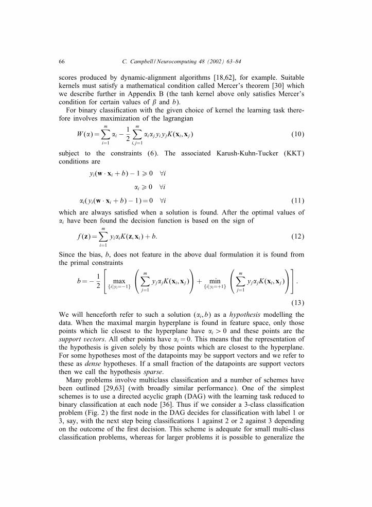
To introduce the subject we will begin by outlining the application of SVMsto the simplest case of binary classi+cation. From the perspective of statisticallearning theory the motivation for considering binary classi+er SVMs comes fromtheoretical bounds on the generalization error [58,11] (the theoretical generaliza-tion performance on new data). These generalization bounds have two importantfeatures (Appendix A). Firstly, the upper bound on the generalization error doesnot depend on the dimension of the space. Secondly, the error bound is minimizedby maximizing the margin, �, i.e. the minimal distance between the hyperplaneseparating the two classes and the closest datapoints to the hyperplane (Fig. 1).

Let us consider a binary classi+cation task with datapoints xi (i = 1; : : : ; m) hav-ing corresponding labels yi =± 1 and let the decision function be

f(x) = sign(w · x + b): (1)

If the dataset is separable then the data will be correctly classi+ed if yi(w · xi +b)¿ 0 ∀i. Clearly this relation is invariant under a positive rescaling of the ar-gument inside the sign-function, hence we implicitly de+ne a scale for (w; b) togive canonical hyperplanes such that w · x + b= 1 for the closest points on oneside and w · x + b= − 1 for the closest on the other side. For the separating hy-perplane w · x + b= 0 the normal vector is clearly w=‖w‖2, and hence the margincan be found from the projection of x1 − x2 onto this vector (see Fig. 1). Sincew ·x1 +b= 1 and w ·x2 +b=−1 this means the margin is �= 1=‖w‖2. To maximize

Fig. 1. The perpendicular distance between the separating hyperplane and a hyperplane through theclosest points (the support vectors) is called the margin. x1 and x2 are examples of support vectorsof opposite sign.

C. Campbell / Neurocomputing 48 (2002) 63–84 65

the margin the task is therefore

minimize g(w) = 12‖w‖2

2 (2)

subject to the constraints

yi(w · xi + b)¿ 1 ∀i (3)

and the learning task can be reduced to minimization of the primal lagrangian

L= 12(w · w)−

m∑i=1

�i(yi(w · x + b)− 1); (4)

where �i are Lagrangian multipliers (hence �i¿ 0). From Wolfe’s theorem [66]we can take the derivatives with respect to b and w and resubstitute back in theprimal to give the Wolfe dual lagrangian

W (�) =m∑i=1

�i − 12

m∑i; j=1

�i�jyiyj(xi · xj) (5)

which must be maximized with respect to the �i subject to the constraints

�i¿ 0m∑i=1

�iyi = 0: (6)

So far we have not used the second feature implied by the generalization theoremmentioned above: the bound does not depend on the dimensionality of the space.For the dual lagrangian (5) we notice that the datapoints, xi ; only appear insidean inner product. To get a better representation of the data we can therefore mapthe datapoints into an alternative higher-dimensional space, called feature space,through a replacement

xi · xj → �(xi) · �(xj): (7)

The functional form of the mapping �(xi) does not need to be known since itis implicitly de+ned by the choice of kernel: K(xi ;xj) =�(xi) · �(xj) or innerproduct in feature space (feature space must therefore be a pre-Hilbert or innerproduct space). With a suitable choice of kernel the data can become separable infeature space despite being non-separable in the original input space: hence kernelsubstitution provides a route for obtaining non-linear algorithms from algorithmspreviously restricted to handling linearly separable datasets. Thus, for example,whereas data for n-parity or the two spirals problem is non-separable by a hy-perplane in input space it can be separated in the feature space de+ned by RBFkernels (giving an RBF-type network)

K(xi ;xj) = e−(xi−xj)2=2�2: (8)

Many other choices for the kernel function are possible, e.g.

K(xi ;xj) = (xi · xj + 1)d K(xi ;xj) = tanh(�xi · xj + b) (9)

de+ning polynomial and feedforward neural network classi+ers. Indeed, the classof mathematical objects which can be used as kernels is very general, and includes


scores produced by dynamic-alignment algorithms [18,62], for example. Suitablekernels must satisfy a mathematical condition called Mercer’s theorem [30] whichwe describe further in Appendix B (the tanh kernel above only satis+es Mercer’scondition for certain values of � and b).

For binary classi+cation with the given choice of kernel the learning task there-fore involves maximization of the lagrangian

W (�) =m∑i=1

�i − 12

m∑i; j=1

�i�jyiyjK(xi ;xj) (10)

subject to the constraints (6). The associated Karush-Kuhn-Tucker (KKT)conditions are

yi(w · xi + b)− 1¿ 0 ∀i�i¿ 0 ∀i

�i(yi(w · xi + b)− 1) = 0 ∀i (11)

which are always satis+ed when a solution is found. After the optimal values of�i have been found the decision function is based on the sign of

f(z) =m∑i=1

yi�iK(z;xi) + b: (12)

Since the bias, b, does not feature in the above dual formulation it is found fromthe primal constraints

b=− 12

max

{i|yi=−1}

m∑

j=1

yj�jK(xi ;xj)

+ min

{i|yi=+1}

m∑

j=1

yj�jK(xi ;xj)

:

(13)

We will henceforth refer to such a solution (�i; b) as a hypothesis modelling thedata. When the maximal margin hyperplane is found in feature space, only thosepoints which lie closest to the hyperplane have �i ¿ 0 and these points are thesupport vectors. All other points have �i = 0. This means that the representation ofthe hypothesis is given solely by those points which are closest to the hyperplane.For some hypotheses most of the datapoints may be support vectors and we refer tothese as dense hypotheses. If a small fraction of the datapoints are support vectorsthen we call the hypothesis sparse.

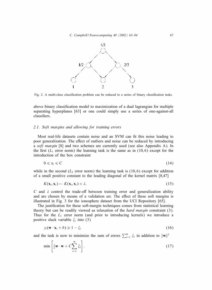
Many problems involve multiclass classi+cation and a number of schemes havebeen outlined [29,63] (with broadly similar performance). One of the simplestschemes is to use a directed acyclic graph (DAG) with the learning task reduced tobinary classi+cation at each node [36]. Thus if we consider a 3-class classi+cationproblem (Fig. 2) the +rst node in the DAG decides for classi+cation with label 1 or3, say, with the next step being classi+cations 1 against 2 or 2 against 3 dependingon the outcome of the +rst decision. This scheme is adequate for small multi-classclassi+cation problems, whereas for larger problems it is possible to generalize the


Fig. 2. A multi-class classi+cation problem can be reduced to a series of binary classi+cation tasks.

above binary classi+cation model to maximization of a dual lagrangian for multipleseparating hyperplanes [63] or one could simply use a series of one-against-allclassi+ers.

2.1. Soft margins and allowing for training errors

Most real-life datasets contain noise and an SVM can +t this noise leading topoor generalization. The e=ect of outliers and noise can be reduced by introducinga soft margin [8] and two schemes are currently used (see also Appendix A). Inthe +rst (L1 error norm) the learning task is the same as in (10; 6) except for theintroduction of the box constraint

06 �i6C (14)

while in the second (L2 error norm) the learning task is (10; 6) except for additionof a small positive constant to the leading diagonal of the kernel matrix [8,47]

K(xi ;xi)← K(xi ;xi) + �: (15)

C and � control the trade-o= between training error and generalization abilityand are chosen by means of a validation set. The e=ect of these soft margins isillustrated in Fig. 3 for the ionosphere dataset from the UCI Repository [65].

The justi+cation for these soft-margin techniques comes from statistical learningtheory but can be readily viewed as relaxation of the hard margin constraint (3).Thus for the L1 error norm (and prior to introducing kernels) we introduce apositive slack variable �i into (3)

yi(w · xi + b)¿ 1− �i (16)

and the task is now to minimize the sum of errors∑m

i=1 �i in addition to ‖w‖2

min

[12w · w + C

m∑i=1

�i

]: (17)


Fig. 3. Left: Test error as a percentage (y-axis) versus C (x-axis) and Right: test error as a percentage(y-axis) versus � (x-axis) for soft margin classi+ers based on L1 and L2 error norms, respectively.The UCI ionosphere dataset was used with RBF kernels (� = 1:5) and 100 samplings of the data.

This is readily formulated as a primal objective function

L(w; b; �; �) = 12w · w + C

m∑i=1

�i −m∑i=1

�i[yi(w · xi + b)− 1 + �i]−m∑i=1

ri�i

(18)

with Lagrange multipliers �i¿ 0 and ri¿ 0. The derivatives with respect to w, band � give

@L@w

=w−m∑i=1

�iyixi = 0; (19)

@L@b

=m∑i=1

�iyi = 0; (20)

@L@�i

=C − �i − ri = 0: (21)

Resubstituting these back in the primal-objective function we obtain the samedual-objective function, (10), as before. However, ri¿ 0 and C−�i− ri = 0, hence�i6C and the constraint 06 �i is replaced by 06 �i6C. Patterns with values0¡�i ¡C will be referred to as non-bound and those with �i = 0 or �i =C will besaid to be at bound. For an L1 error norm we +nd the bias in the decision function(12) from the KKT conditions for the soft margin case. In particular ri�i = 0 and�i(yi(w · xi + b) − 1 + �i) = 0, hence if we select a non-bound datapoint i (suchthat 0¡�i ¡C) we +nd from C − �i − ri = 0 that ri ¿ 0 hence �i = 0, and since�i ¿ 0 so can determine b from b=yi − w · xi assuming yi =± 1.

The optimal value of C must be found by experimentation using a validation setand it cannot be readily related to the characteristics of the dataset or model. In an


alternative approach (�-SVM [45]) it can be shown that solutions for an L1-errornorm are the same as those obtained from maximizing

W (�) =− 12

m∑i; j=1

�i�jyiyjK(xi ;xj) (22)

subject tom∑i=1

yi�i = 0m∑i=1

�i¿ � 06 �i61m; (23)

where � lies on the range 0 to 1. The fraction of training errors is upper boundedby � and � also provides a lower bound on the fraction of points which are sup-port vectors. Hence in this formulation the conceptual meaning of the soft marginparameter is more transparent.

For the L2 error norm the primal objective function is

L(w; b; �; �) = 12w · w + C

m∑i=1

�2i −

m∑i=1

�i[yi(w · xi + b)− 1 + �i]−m∑i=1

ri�i

(24)

with �i¿ 0 and ri¿ 0. After obtaining the derivatives with respect to w, b and �,substituting for w and � in the primal objective function and noting that the dualobjective function is maximal when ri = 0; we obtain the following dual objectivefunction after kernel substitution

W (�) =m∑i=1

�i − 12

m∑i; j=1

yiyj�i�jK(xi ;xj)− 14C

m∑i=1

�2i : (25)

With �= 1=2C this gives the same dual objective function as for hard marginlearning except for the substitution (15). For many real-life datasets there is animbalance between the amount of data in di=erent classes, or the signi+cance ofthe data in the two classes can be quite di=erent. For example, for the detection oftumours on MRI scans it may be best to allow a higher number of false positivesif this improved the true positive detection rate. The relative balance betweenthe detection rate for di=erent classes can be easily shifted [59] by introducingasymmetric soft margin parameters. Thus for binary classi+cation with an L1

error norm 06 �i6C+ (yi = + 1), and 06 �i6C−(yi =− 1), while K(xi ;xi)←K(xi ;xi) + �+ (if yi = + 1) and K(xi ;xi)← K(xi ;xi) + �− (if yi =− 1) for the L2

error norm.

2.2. A linear programming approach to classi3cation

Rather than using quadratic programming it is also possible to derive a kernelclassi+er in which the learning task involves linear programming (LP) instead.Training the classi+er involves the minimization

min

[m∑i=1

�i + Cm∑i=1

�i

](26)


subject to

yi

m∑

j=1

�iK(xi; xj) + b

¿ 1− �i; (27)

where �i¿ 0 and �i¿ 0. By minimizing∑m

i=1 �i we could obtain a solution whichis sparse i.e. relatively fewer datapoints are used. Furthermore, eMcient simplexor column-generation techniques exist for solving linear programming problemsso this is a practical alternative to conventional QP SVMs. This linear program-ming approach evolved independently of the QP approach to SVMs [27] and, aswe will see, linear programming approaches to regression and novelty detectionare also possible. It is also possible to handle multi-class problems using linearprogramming [63].

2.3. Model selection

Apart from the choice of kernel, the other indeterminate is the choice of thekernel parameter (e.g. � in (8)). The kernel parameter can be found using cross-validation if suMcient data is available. However, recent model-selection strategiescan give a reasonable estimate for the kernel parameter without use of additionalvalidation data. As a +rst attempt we can use a theorem stating that the general-ization error bound is reduced as the margin � is increased. This theorem givesthe upper bound as R2=m�2 where R is the radius of the smallest ball containingthe training data. At an optimum of (10) it is possible to show that �2 = 1=

∑i �

0i

(where �0i are the values of �i at the optimum). Also for RBF kernels it is fre-

quently the case that R � 1 (since the data lies on the surface of hyperspherefrom �(x) ·�(x) =K(x;x) = 1) so the bound can be written

∑mi=1 �0

i =m. Hence anestimate for � can be found by sequentially training SVMs on the same datasetat successively larger values of �, evaluating the bound from the �0

i for each caseand choosing that value of � for which the bound is minimized. This method [10]will give a reasonable estimate if the data is spread evenly over the surface ofthe hypersphere but it is poor if the data lie in a Oat ellipsoid, for example, sincethe radius R would be inOuenced by the largest deviations. More re+ned estimatestherefore take into account the distribution of the data.

One approach [6] is to theoretically rescale data in feature space to compensatefor uneven distributions. A more complex strategy along these lines has also beenproposed by SchPolkopf et al. [44] which leads to an algorithm which has performedwell in practice for a small number of datasets. The most economical way to usethe training data is to use a leave-one-out procedure [6,21]. As an example, weconsider a recent result [22,56] in which the number of leave-one-out errors of anL1-norm soft margin SVM is bounded by |{i: (2�iB2 +�i)¿ 1}|=m where �i are thesolutions of the optimization task in (10; 6) and B2 is an upper bound on K(xi; xi)with K(xi; xj)¿ 0 (we can determine �i from yi(

∑j �jK(xj; xi)+b)¿ 1−�i). Thus,

for a given value of the kernel parameter, the leave-one-out error is estimatedfrom this quantity (the system is not retrained with datapoints left out: the bound


is determined using the �0i from the solution of (10; 6)). The kernel parameter is

then incremented or decremented in the direction needed to lower the bound. Thismethod has worked well on classi+cation of text [22].

2.4. Novelty detection

For many real-world problems the task is not to classify but to detect novel orabnormal instances. Novelty or abnormality detection has potential applications inmany problem domains such as condition monitoring or medical diagnosis. Oneapproach can be viewed as one-class classi+cation in which the task is to model thesupport of a data distribution (rather than having to +nd a real-valued function forestimating the density of the data itself). Thus, at its simplest level, the objectiveis to create a binary-valued function which is positive in those regions of inputspace where the data predominantly lies and negative elsewhere.

One strategy [52] is to +nd a hypersphere with a minimal radius R and center awhich contains most of the data: novel test points lie outside the boundary of thishypersphere. The technique we now outline was originally suggested by Burges[40,3], intepreted as a novelty detector by Tax and Duin [52] and used by thelatter authors for real life applications [53]. The e=ect of outliers is reduced byusing slack variables �i to allow for datapoints outside the sphere and the task isto minimize the volume of the sphere and number of datapoints outside i.e.

min

[R2 +

1m�

∑i

�i

](28)

subject to the constraints

(xi − a)T(xi − a)6R2 + �i (29)

and �i¿ 0, and where � controls the tradeo= between the two terms. The primalobjective function is then

L(R; a; �i; �i) = R2 +1m�

m∑i=1

�i −m∑i=1

�i�i

−m∑i=1

�i(R2 + �i − (xi · xi − 2a · xi + a · a)) (30)

with �i¿ 0 and �i¿ 0. After kernel substitution the dual formulation amounts tomaximization of

W (�) =m∑i=1

�iK(xi ;xi)−m∑

i; j=1

�i�jK(xi ;xj) (31)

with respect to �i and subject to∑m

i=1 �i = 1 and 06 �i6 1=m�. If m�¿ 1 then atbound examples will occur with �i = 1=m� and these correspond to outliers in thetraining process. Having completed the training process a test point z is declared


novel if

K(z; z)− 2m∑i=1

�iK(z;xi) +m∑

i; j=1

�i�jK(xi ;xj)− R2¿ 0; (32)

where R2 is +rst computed by +nding an example which is non-bound and settingthis inequality to an equality.

An alternative approach has been developed by SchPolkopf et al. [43]. Supposewe restrict our attention to RBF kernels then the datapoints lie on the surface of ahypersphere in feature space since �(x) · �(x) =K(x;x) = 1 from (8). The objec-tive is to separate o= the region containing the datapoints from the surface regioncontaining no data. This is achieved by constructing a hyperplane which is maxi-mally distant from the origin with all datapoints lying on the opposite side from theorigin and such that w · xi + b¿ 0. This approach leads to an alternative quadraticprogramming problem and the authors [43] report that the technique works wellon real-life datasets, including the highlighting of abnormal digits for the USPShandwritten character dataset. Instead of repelling the hyperplane away from theorigin a further alternative is to attract the hyperplane towards the datapoints infeature space (while maintaining the requirement w · xi + b¿ 0). This leads to analgorithm for novelty detection based on linear programming [4].

3. Regression

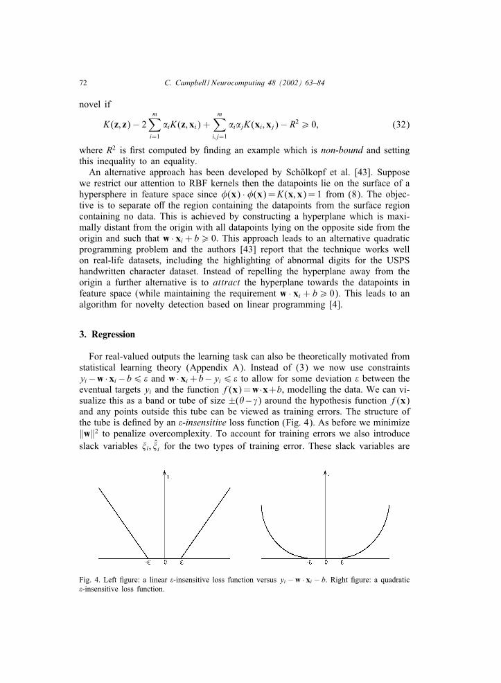
For real-valued outputs the learning task can also be theoretically motivated fromstatistical learning theory (Appendix A). Instead of (3) we now use constraintsyi−w ·xi−b6 ! and w ·xi +b−yi6 ! to allow for some deviation ! between theeventual targets yi and the function f(x) =w·x+b, modelling the data. We can vi-sualize this as a band or tube of size ±("−�) around the hypothesis function f(x)and any points outside this tube can be viewed as training errors. The structure ofthe tube is de+ned by an !-insensitive loss function (Fig. 4). As before we minimize‖w‖2 to penalize overcomplexity. To account for training errors we also introduceslack variables �i; �̂i for the two types of training error. These slack variables are

Fig. 4. Left +gure: a linear !-insensitive loss function versus yi − w · xi − b. Right +gure: a quadratic!-insensitive loss function.


zero for points inside the tube and progressively increase for points outside thetube according to the loss function used. This general approach is called !-SVregression [57] and is the most common approach to SV regression, though notthe only one [58]. For a linear !-insensitive loss function the task is therefore tominimize

min

[‖w‖2 + C

m∑i=1

(�i + �̂i)

](33)

subject to

yi − w · xi − b6 ! + �i;

(w · xi + b)− yi6 ! + �̂i; (34)

where the slack variables are both positive �i; �̂i¿ 0. After kernel substitution thedual objective function is

W (�; �̂) =m∑i=1

yi(�i − �̂i)− !m∑i=1

(�i + �̂i)− 12

m∑i; j=1

(�i − �̂i)(�j − �̂j)K(xi; xj)

(35)

which is maximized subject tom∑i=1

�̂i =m∑i=1

�i (36)

and

06 �i6C 06 �̂i6C: (37)

Similarly a quadratic !-insensitive loss function gives rise to

min

[‖w‖2 + C

m∑i=1

(�2i + �̂

2i )

](38)

subject to (34), giving a dual objective function

W (�; �̂) =m∑i=1

yi(�i − �̂i)− !m∑i=1

(�i + �̂i)

− 12

m∑i; j=1

(�i − �̂i)(�j − �̂j)(K(xi ;xj) + #ij=C) (39)

which is maximized subject to (36). The function modelling the data is then

f(z) =m∑i=1

(�i − �̂i)K(xi ; z) + b: (40)


We still have to compute the bias, b, and we do so by considering KKT conditionsfor regression. For a linear loss function prior to kernel substitution these are

�i(! + �i − yi + w · xi + b) = 0;

�̂i(! + �̂i + yi − w · xi − b) = 0; (41)

where w=∑m

j=1 yj(�j − �̂j)xj, and

(C − �i)�i = 0;

(C − �̂i)�̂i = 0: (42)

From the latter conditions we see that only when �i =C or �̂i =C are the slackvariables non-zero: these examples correspond to points outside the !-insensitivetube. Hence from (41) we can +nd the bias from a non-bound example with0¡�i ¡C using b=yi −w · xi − ! and similarly for 0¡�̂i ¡C we can obtain itfrom b=yi − w · xi + !. Though the bias can be obtained from one such exampleit is best to compute it using an average over all points on the margin.

Apart from the formulations given here it is possible to de+ne other loss func-tions giving rise to di=erent dual objective functions. In addition, rather than spec-ifying ! a priori it is possible to specify an upper bound � (06 �6 1) on thefraction of points lying outside the band and then +nd ! by optimizing over theprimal objective function

12‖w‖2 + C

(�m! +

m∑i=1

|yi − f(xi)|)

(43)

with ! acting as an additional parameter to minimize over [39]. As for classi+cationand novelty detection it is possible to formulate a linear programming approach toregression with [64]

min

[m∑i=1

�i +m∑i=1

�∗i + Cm∑i=1

�i + Cm∑i=1

�∗i

](44)

subject to

yi − !− �i6

m∑

j=1

(�∗j − �j)K(xi; xj)

+ b6yi + ! + �∗i : (45)

Minimizing the sum of the �i approximately minimizes the number of supportvectors which favours sparse hypotheses with smooth functional approximationsof the data. In this approach the kernel does not need to satisfy Mercer’scondition [64].

4. Algorithmic approaches

So far the methods we have considered have involved linear or quadratic pro-gramming. Linear programming can be implemented using column generation tech-niques [32] and many packages are available, e.g. CPLEX. Existing LP packages


based on simplex or interior point methods can handle problems of moderate size(up to thousands of datapoints). For quadratic programming there are also manyapplicable techniques including conjugate gradient and primal-dual interior pointmethods [26]. Certain QP packages are readily applicable such as MINOS andLOQO. These methods can be used to train an SVM rapidly but they have thedisadvantage that the kernel matrix is stored in memory. For small datasets thisis practical and QP routines are the best choice, but for larger datasets alterna-tive techniques have to be used. These split into three categories: techniques inwhich kernel components are evaluated and discarded during learning, working setmethods in which an evolving subset of data is used, and new algorithms thatexplicitly exploit the structure of the problem. For the +rst category the most obvi-ous approach is to sequentially update the �i and this is the approach used by thekernel adatron (KA) algorithm [15]. For binary classi+cation (with no soft marginor bias) this is a simple gradient ascent procedure on (10) in which �i¿ 0 initiallyand the �i are subsequently sequentially updated using

�i ← �i"(�i); where �i = �i + $

1− yi

m∑j=1

�jyjK(xi ;xj)

(46)

and "(�) is the heaviside step function. The optimal learning rate $ can be readilyevaluated: $= 1=K(xi ;xi) and a suMcient condition for convergence is 0¡$K(xi ;xi)¡ 2. With the decision function (12) this method is very easy to implement andcan give a quick impression of the performance of SVMs on classi+cation tasks.It can be generalized to the case of soft margins and inclusion of a bias [26,5].However, it is not as fast as most QP routines, especially on small datasets.

Chunking and decomposition. Rather than sequentially updating the �i the al-ternative is to update the �i in parallel but using only a subset or chunk of dataat each stage. Thus a QP routine is used to optimize the lagrangian on an initialarbitrary subset of data. The support vectors found are retained and all other dat-apoints (with �i = 0) discarded. A new working set of data is then derived fromthese support vectors and additional datapoints which maximally violate the storageconstraints. This chunking process is then iterated until the margin is maximized.Of course, this procedure may still fail because the dataset is too large or thehypothesis modelling the data is not sparse (most of the �i are non-zero, say). Inthis case decomposition [34] methods provide a better approach: these algorithmsonly use a +xed size subset of data with the �i for the remainder kept +xed.

Decomposition and sequential minimal optimization (SMO). The limiting caseof decomposition is the sequential minimal optimization (SMO) algorithm of Platt[35] in which only two �i are optimized at each iteration. The smallest set ofparameters which can be optimized with each iteration is plainly two if the con-straint

∑mi=1 �iyi = 0 is to hold. Remarkably, if only two parameters are optimized

and the rest kept +xed then it is possible to derive an analytical solution whichcan be executed using few numerical operations. The method therefore consistsof a heuristic step for +nding the best pair of parameters to optimize and use ofan analytic expression to ensure the lagrangian increases monotonically. For the


hard margin case the latter is easy to derive from the maximization of #W withrespect to the additive corrections a; b in �i → �i + a and �j → �j + b; (i �= j). Forthe L1 soft margin care must be taken to avoid violation of the constraints (14)leading to bounds on these corrections. The SMO algorithm has been re+ned toimprove speed [24] and generalized to cover the above above-mentioned tasks ofclassi+cation [35], regression [48] and novelty detection [43]. SVM packages suchas SVMTorch [7] and SVMLite [23] also use these working set methods. Thereare also interesting LP variants for these decomposition methods. The fastest LPmethods decompose the problem by rows and columns and have been used tosolve the largest reported non-linear SVM regression problem with up to 16000datapoints and a kernel matrix with over a billion elements [2].

Further optimization algorithms. The third approach is to directly approachtraining from an optimization perspective and create new algorithms. Keerthi etal. [25] have proposed a very e=ective binary classi+cation algorithm based onthe dual geometry of +nding the two closest points in the convex hulls. Theseapproaches have been particularly e=ective for linear SVM problems. The La-grangian SVM (LSVM) method of Mangasarian and Musicant [28] reformulatesthe classi+cation problem as an unconstrained optimization task and then solvesthe problem using an algorithm which only requires the solution of systems oflinear equalities. Using a simple program, LSVM can solve linear classi+cationproblems for millions of points in minutes. LSVM uses a method based on theSherman-Morrison-Woodbury formula which only requires solution of systems oflinear equalities. The interior-point [13] and semi-smooth support vector methods[14] of Ferris and Munson can be used to solve linear classi+cation problems withup to 60 million data points in 34 dimensions.

5. Further techniques based on kernel representations

So far we have considered methods based on linear and quadratic programming.Here we shall consider further kernel-based approaches which may utilize generalnon-linear programming and other techniques. In particular, we will consider ap-proaches to two issues: how to improve generalization performance over standardSVMs and how to create hypotheses which are sparse.

Algorithms leading to dense hypotheses. Taking the geometric dual of inputspace we +nd datapoints become hyperplanes and separating hyperplanes becomepoints. In this dual space we de+ne version space as the set of all hypotheses(points) consistent with the data and this version space is bounded by the hyper-planes representing the data. An SVM solution can be viewed as the center of thelargest inscribable hypersphere in version space: the support vectors correspond tothose examples with hyperplanes tangentially touching this hypersphere (Fig. 5).If version space is elongated then the center of the largest inscribed hyperspheredoes not appear to be the best choice. Indeed, a better choice would be the Bayespoint which can be approximated by the center of mass of version space [61].Bayes point machines (BPMs) construct a hypothesis based on this center of ver-


Fig. 5. The center of mass of version space (×) and the center of the largest inscribed sphere (+) inan elongated version space.

sion space and this choice can be justi+ed by theoretical arguments [33,61,38] inaddition to having a geometric appeal. In one approach the center of mass is de-termined using a kernelized billiard algorithm in which version space is traverseduniformly and an estimate of the center of mass is repeatedly updated. For a largemajority of datasets version space diverges from sphericality and the BPM outper-forms an SVM at statistically signi+cant levels. For arti+cial examples with veryelongated version spaces the generalization error of a BPM can be half that of anSVM [19,20].

Rather than using the center of mass of version space an alternative might beto use a hypothesis that lies towards the center of this space but which is easierto compute. This could be achieved by using repulsive potentials )(�) favouringpoints towards the center of version space [38]. As an example we could use

min)(�) =

[m∑i=1

ln(�iK(xi; xj) + b)

](47)

subject to12

m∑i=1

�2i = 1 (48)

which is the basis of the analytic center machine (ACM) [55]. The gradient andHessian for (47) can be readily evaluated allowing for computational eMciency andthe algorithm appears to perform well in practice. Training involves optimizationof a non-linear function and leads to a dense hypothesis.

The ACM algorithm is one example of a broad class of algorithms to which ker-nel substitution can be applied and which lead to a non-QP non-linear programming


task for training. The hypotheses constructed are typically dense in the number ofsupport vectors. For example, for classi+cation, the idea of kernel substitution canbe readily applied to the Fisher discriminant [12] and the resulting classi+er workswell in practice [31]. For regression one can similarly apply kernel substitution tominimization of the standard least squares error function based on the di=erencebetween target and the output of the regression function [37,50,51]. This leads tonon-linear regression (and classi+cation) functions which perform well on real-lifedatasets.

Generating sparse hypotheses. The Bayes point machine may exhibit good gen-eralization but it has the disadvantage that the hypothesis is dense. Ideally we wouldalso like to derive kernel classi+ers or regression machines which give sparse hy-potheses using a minimal number of datapoints. The most e=ective means of ob-taining sparse hypotheses remains an object of research but an excellent scheme isthe relevance vector machine of Tipping [54]. Using the function f(z) =∑m

i=1 �iK(z; xi) + b to model the data, a Bayesian prior is de+ned over the modelparameters favouring smooth sparse hypotheses. From Bayes rule a posterior overthe weights can be obtained and thence a marginal likelihood or evidence. Iterativemaximization of this evidence suggests suitable examples for pruning, creating aneventual hypothesis which is sparse in the number of datapoints used. Experimentsshow that this approach can sometimes give hypotheses which only use a fewpercent of the available data [54].

6. Conclusion

The approach we have considered is very general in that it can be applied toa wide range of machine learning tasks and can be used to generate many possi-ble learning machine architectures (RBF networks, feedforward neural networks)through an appropriate choice of kernel. A variety of optimization techniques canbe used during the training process which typically involves optimization of a con-vex function. Above all, kernel methods have been found to work well in practice.The subject is still very much under development but it can be expected to developas an important tool for machine learning and applications.

Appendix A. Generalization bounds

The generalization bounds mentioned in Section 2 are derived within the frame-work of probably approximately correct (pac) learning. The training and test dataare assumed independently and identically (iid) generated from a +xed distri-bution denoted D. The distribution over input–output mappings will be denoted(x; y)∈X ×{−1; 1} with X assumed to be an inner product space. With these as-sumptions pac-learnability can be de+ned as follows. Consider a class of possibletarget concepts C and a learner L using a hypothesis space H to try and learn thisconcept class. Given a suMcient number, m, of training examples the class C is


pac-learnable by L if for any target concept c∈C; L will with probability (1− #)output a hypothesis h∈H with a generalization error errD(h)¡!(m;H; #). The pacbound !(m;H; #) is derived using probabilistic arguments [1,60] and bounds the tailof the distribution of the generalization error errD(h).

For the case of a thresholding learner L with unit weight vector on an innerproduct space X and a margin �∈R+ the following theorem can be derived if thedataset is linearly separable:

Theorem 1. Suppose examples are drawn independently according to a distribu-tion whose support is contained in a ball in Rn centered at the origin; of radius R.If we succeed in correctly classifying m such examples by a canonical hyperplane;then with con3dence 1 − # the generalization error will be bounded from aboveby [46]

!(m;H; #) =2m

(64R2

�2 log(�em

8R2

)log(

32m�2

)+ log

(4#

))(49)

provided 64R2=�2 ¡m. This result does not depend on the dimensionality of thespace and also states that the bound is reduced by maximizing the margin �.

Though this is our main result motivating maximization of the margin for SVMsit does not handle the case of non-separable data or the existence of noise. Aspointed out in the main text these instances are handled by introducing an L1 orL2 soft margin. The following two bounds do not depend on the training data beinglinearly separable and cover these two cases [47]:

Theorem 2. Suppose examples are drawn independently according to a distribu-tion whose support is contained in a ball in Rn centered at the origin; of radiusR. There is a constant c such that with con3dence 1− # the generalization errorwill be bounded from above by

!(m;H; #) =cm

(R2 + ‖�‖2

1 log(1=�)�2 log2(m) + log

(1#

)); (50)

where � is the margin slack vector.

Theorem 3. Suppose examples are drawn independently according to a distribu-tion whose support is contained in a ball in Rn centered at the origin; of radiusR. There is a constant c such that with con3dence 1− # the generalization errorwill be bounded from above by

!(m;H; #) =cm

(R2 + ‖�‖2

2

�2 log2(m) + log(

1#

)); (51)

where � is the margin slack vector.

For both these theorems we see that maximizing the margin alone does notnecessarily reduce the bound and it is necessary to additionally reduce the normsof the slack variables.


Both these theorems can be adapted to the case of regression. However, incontrast to Theorems 1–3 above it is no longer appropriate to +x the norm of theweight vector since invariance under positive rescaling of the weight vector onlyholds for a thresholding decision function. For regression the relevant theorem foran L2 norm on the slack variables is then:

Theorem 4. Suppose examples are drawn independently according to a distribu-tion whose support is contained in a ball in Rn centered at the origin; of radiusR. Furthermore 3x �6 " where " is a positive real number. There is a constantc such that with probability 1− # over m random examples; the probability thata hypothesis with weight vector w has output more than " away from its truevalue is bounded above by

!(m;H; #) =cm

(‖w‖22R

2 + ‖�‖22

�2 log2(m) + log(

1#

)); (52)

where �= �(w; "; �) is the margin slack vector. This theorem motivates the lossfunctions for regression.

Appendix B. Kernel substitution and Mercer’s theorem

In Section 2 we introduced the idea of kernel substitution, equivalent to in-troducing an implicit mapping of the data into a high-dimensional feature space.Non-linear datasets which are unlearnable by a linear learning machine in inputspace can then become learnable in feature space. In input space the hypothesismodelling the data is of the form

f(x) =w · x + b: (53)

If the dataset is separable, the separating hyperplane passes through the convexhull de+ned by the datapoints and hence w can be expressed as an expansion interms of the datapoints thus

w=m∑i=1

�iyixi : (54)

With this expansion the decision function can therefore be written

f(x) =m∑i=1

�iyi(xi · xj) + b: (55)

The xi only appear inside an inner product, justifying kernel substitution and withthe choice of kernel implicitly selecting a particular feature space

K(xi ;xj) =�(xi) · �(xj): (56)

However, only certain choices of kernel are allowable. The requirements on thekernel function are de+ned by the two theorems below. First we observe that the


kernel function is symmetric. In addition we also note from that for a real vectorv we have

vTKv=

∥∥∥∥∥m∑i=1

vTi �(xi)

∥∥∥∥∥2

2

¿ 0; (57)

where the matrix K has components K(xi ;xj); (i = 1; : : : ; m; j = 1; : : : ; m). This sug-gests the following theorem which can be proved:

Theorem 5. Let K(x; y) be a real symmetric function on a 3nite input space; thenit is a kernel function if and only if the matrix K with components K(xi ;xj) ispositive semi-de3nite.

More generally, for C a compact subset of RN we have:

Theorem 6 (Mercer’s theorem). If K(x; y) is a continuous symmetric kernel of apositive integral operator T i.e.

(Tf)(y) =∫CK(x; y)f(x) dx (58)

with ∫C×C

K(x; y)f(x)f(y) dxdy¿ 0 (59)

for all f∈L2(C) then it can be expanded in a uniformly convergent series in theeigenfunctions j and positive eigenvalues �j of T; thus

K(x; y) =ne∑j=1

�j j(x) j(y); (60)

where ne is the number of positive eigenvalues.

This theorem holds for general compact spaces, and generalizes the requirementto in+nite feature spaces. (59) generalizes the semi-positivity condition given inTheorem 5 above.

References

[1] M. Anthony, P. Barlett, Learning in neural networks: theoretical foundations, CambridgeUniversity Press, Cambridge, 1999.

[2] P. Bradley, O. Mangasarian, D. Musicant, Optimization in massive datasets, in: J. Abello,P. Pardalos, M. Resende (Eds.), Handbook of Massive Datasets, Kluwer, Dordrecht, 2001,to appear.

[3] C. Burges, A tutorial on support vector machines for pattern recognition, Data Mining andKnowledge Discovery 2 (1998) 121–167.

[4] C. Campbell, K.P. Bennett, A linear programming approach to novelty detection, Advances inNeural Information Processing Systems, vol. 13, MIT Press, Cambridge, MA, 2001, 395–401.


[5] C. Campbell, N. Cristianini, Simple training algorithms for support vector machines, TechnicalReport, Bristol University, http:==lara.enm.bris.ac.uk=cig, 1998.

[6] O. Chapelle, V. Vapnik, Model selection for support vector machines, to appear in Advances inNeural Information Processing Systems, vol. 12, MIT Press, Cambridge, MA, 2000.

[7] R. Collobert, S. Bengio, SVMTorch web page: http:==www.idiap.ch=learning=SVMTorch.html.[8] C. Cortes, V. Vapnik, Support vector networks, Machine Learning 20 (1995) 273–297.[9] N. Cristianini, C. Campbell, C. Burges (Eds.), Support vector machines and kernel methods,

Machine Learning, 2001, to appear.[10] N. Cristianini, C. Campbell, J. Shawe-Taylor, Dynamically adapting kernels in support vector

machines, Advances in Neural Information Processing Systems, vol. 11, MIT Press, Cambridge,MA, 1999, pp. 204–210.

[11] N. Cristianini, J. Shawe-Taylor, An introduction to support vector machines and other kernel-basedlearning methods, Cambridge University Press, Cambridge, 2000.

[12] R.O. Duda, P.E. Hart, Pattern classi+cation and scene analysis, Wiley, New York, 1973.[13] M. Ferris, T. Munson, Interior point methods for massive support vector machines, Data Mining

Institute Technical Report 00-05, Computer Sciences Department, University of Wisconsin,Madison, Wisconsin, 2000.

[14] M. Ferris, T. Munson, Semi-smooth support vector machines, Data Mining Institute TechnicalReport 00-09, Computer Sciences Department, University of Wisconsin, Madison, Wisconsin,2000.

[15] T.-T. Friess, N. Cristianini, C. Campbell, The kernel adatron algorithm: a fast and simple learningprocedure for support vector machines. 15th International Conference on Machine Learning,Morgan Kaufman Publishers, 1998, pp. 188–196.

[16] I. Guyon, N. Matic, V. Vapnik, Discovering informative patterns and data cleaning, in:U.M. Fayyad, G. Piatetsky-Shapiro, P. Smyth, R. Uthurusamy (Eds.), Advances in KnowledgeDiscovery and Data Mining, MIT Press, Cambridge, MA, 1996, pp. 181–203.

[17] Cf: http:==www.clopinet.com=isabelle=Projects=SVM=applist.html.[18] D. Haussler, Convolution Kernels on Discrete Structures, UC Santa Cruz Technical Report

UCS-CRL-99-10, 1999.[19] R. Herbrich, T. Graepel, C. Campbell, Bayes Point Machines, J. Machine Learning Res. (2001)

to appear.[20] R. Herbrich, T. Graepel, C. Campbell, Robust bayes point machines, Proceedings of ESANN2000,

D-Facto Publications, Belgium, 2000, pp. 49–54.[21] T. Jaakolla, D. Haussler, Probabilistic kernel regression models, Proceedings of the 1999

Conference on AI and Statistics, 1999.[22] T. Joachims, Estimating the generalization performance of an SVM eMciently, Proceedings

of the Seventeenth International Conference on Machine Learning, Morgan Kaufmann, 2000,pp. 431–438.

[23] T. Joachims, Web Page for SVMLight Software: http:==wwwais.gmd.de= t̃horsten=svm light.[24] S. Keerthi, S. Shevade, C. Bhattacharyya, K. Murthy, Improvements to Platt’s SMO algorithm

for SVM classi+er design, Technical Report, Department of CSA, Bangalore, India, 1999.[25] S. Keerthi, S. Shevade, C. Bhattacharyya, K.A. Murthy, A fast iterative nearest point algorithm

for support vector machine classi+er design, IEEE Trans. Neural Networks 11 (2000) 124–136.[26] D. Luenberger, Linear and Nonlinear Programming, Addison-Wesley, Reading, MA, 1984.[27] O.L. Mangasarian, Linear and non-linear separation of patterns by linear programming, Oper.

Res. 13 (1965) 444–452.[28] O. Mangasarian, D. Musicant, Lagrangian support vector regression, Data mining Institute

Technical Report 00-06, June 2000.[29] E. Mayoraz, E. Alpaydin, Support vector machines for multiclass classi+cation, Proceedings of

the International Workshop on Arti+cial Neural Networks (IWANN99), IDIAP Technical Report98-06, 1999.

[30] J. Mercer, Functions of positive and negative type and their connection with the theory of integralequations, Philos. Trans. Roy. Soc. London A 209 (1909) 415–446.


[31] S. Mika, G. Ratsch, J. Weston, B. SchPolkopf, K.-R. Muller, Fisher discriminant analysiswith kernels, Proceedings of IEEE Neural Networks for Signal Processing Workshop, 1999,pp. 41–48.

[32] S. Nash, A. Sofer, Linear and non-linear programming, McGraw-Hill, New York, 1996.[33] M. Opper, D. Haussler, Generalization performance of bayes optimal classi+cation algorithm for

learning a perceptron, Phys. Rev. Lett. 66 (1991) 2677–2680.[34] E. Osuna, F. Girosi, Reducing the Run-time Complexity in Support Vector Machines, in:

B. SchPolkopf, C. Burges, A. Smola (Eds.), Advances in Kernel Methods: Support Vector Learning,MIT press, Cambridge, MA, 1999, pp. 271–284.

[35] J. Platt, Fast training of SVMs using sequential minimal optimization, in: B. SchPolkopf,C. Burges, A. Smola (Eds.), Advances in Kernel Methods: Support Vector Learning, MIT press,Cambridge, MA, 1999, pp. 185–208.

[36] J. Platt, N. Cristianini, J. Shawe-Taylor, Large margin DAGS for multiclass classi+cation,Advances in Neural Information Processing Systems, vol. 12, MIT Press, Cambridge, MA, 2000.

[37] C. Saunders, A. Gammerman, V. Vovk, Ridge regression learning algorithm in dual variables,Proceedings of the 15th International Conference on Machine Learning (ICML 98), MorganKaufmann, Los Altos, CA, 1998, pp. 515–521.

[38] J. Schietse, Towards Bayesian Learning for the Perceptron, Ph.D. Thesis, FaculteitWetenschappen, Limburgs Universitair Centrum, Belgium, 1996.

[39] B. SchPolkopf, P. Bartlett, A. Smola, R. Williamson, Support vector regression with automaticaccuracy control, in: L. Niklasson, M. BUoden, T. Ziemke (Eds.), Proceedings of the 8thInternational Conference on Arti+cial Neural Networks, Perspectives in Neural Computing,Springer, Berlin, 1998.

[40] B. SchPolkopf, C. Burges, V. Vapnik, Extracting support data for a given task, Proceedings:First International Conference on Knowledge Discovery and Data Mining, in: U.M. Fayyad,R. Uthurusamy (Eds.), AAAI Press, Menlo Park, CA, 1995.

[41] B. SchPolkopf, C. Burges, A. Smola, Advances in Kernel Methods: Support Vector Machines,MIT Press, Cambridge, MA, 1998.

[42] B. SchPolkopf, A. Smola, K.-R. Muller, Kernel Principal Component Analysis, in: B. SchPolkopf,C. Burges, A. Smola (Eds.), Advances in Kernel Methods: Support Vector Machines, MIT Press,Cambridge, MA, 1998, pp. 327–352.

[43] B. SchPolkopf, J.C. Platt, J. Shawe-Taylor, A.J. Smola, R.C. Williamson, Estimating thesupport of a high-dimensional distribution, Microsoft Research Corporation Technical ReportMSR-TR-99-87, 1999.

[44] B. SchPolkopf, J. Shawe-Taylor, A. Smola, R. Williamson, Kernel-dependent support vector errorbounds, Ninth International Conference on Arti+cial Neural Networks, No. 470, IEE ConferencePublications, 1999, pp. 304–309.

[45] B. SchPolkopf, A. Smola, R.C. Williamson, P.L. Bartlett, New support vector algorithms, NeuralComputation 12 (2000) 1207–1245.

[46] J. Shawe-Taylor, P.L. Bartlett, R.C. Williamson, M. Anthony, Structural risk minimization overdata-dependent hierarchies, IEEE Trans. Inform. Theory 44 (1998) 1926–1940.

[47] J. Shawe-Taylor, N. Cristianini, Margin distribution and soft margin, in: A. Smola, P. Barlett, B.SchPolkopf, C. Schuurmans (Eds.), Advances in Large Margin Classi+ers, Chapter 2, MIT Press,Cambridge, MA, 1999.

[48] A. Smola, B. SchPolkopf, A tutorial on support vector regression, NeuroColt2 TR 1998-03, 1998.[49] A. Smola, P. Barlett, B. SchPolkopf, C. Schuurmans (Eds.), Advances in Large Margin Classi+ers,

MIT Press, Cambridge, MA, 2001.[50] J.A.K. Suyhens, J. Vandewalle, Least squares support vector machine classi+ers, Neural Process.

Lett. 9 (1999) 293–300.[51] J.A.K. Suyhens, L. Lukas J. Vandewalle, Sparse approximation using least squares support vector

machines, Proceedings of the IEEE International Symposium on Circuits and Systems, Geneva,Switzerland (2000) II757–II760.

[52] D. Tax, R. Duin, Data domain description by Support Vectors, in: M. Verleysen (Ed.),Proceedings of ESANN99, D. Facto Press, Brussels, 1999, pp. 251–256.


[53] D. Tax, A. Ypma, R. Duin, Support vector data description applied to machine vibration analysis,in: M. Boasson, J. Kaandorp, J. Tonino, M. Vosselman (Eds.), Proceedings of the 5th AnnualConference of the Advanced School for Computing and Imaging, Heijen, NL, June 15–17, 1999,pp. 398–405.

[54] M. Tipping, The Relevance Vector Machine, Advances in Neural Information Processing Systems,vol. 12, MIT Press, Cambridge, MA, 2000, pp. 652–658.

[55] T. Trafalis, A. Malysche=, An analytic center machine, Machine Learning, to appear.[56] V. Vapnik, O. Chapelle, Bounds on error expectation for SVMs, Neural Computation, to appear.[57] V. Vapnik, The Nature of Statistical Learning Theory, Springer, New York, 1995.[58] V. Vapnik, Statistical Learning Theory, Wiley, New York, 1998.[59] K. Veropoulos, C. Campbell, N. Cristianini, Controlling the sensitivity of support vector machines,

Proceedings of the International Joint Conference on Arti+cial Intelligence (IJCAI), Stockholm,Sweden, 1999.

[60] M. Vidyasagar, A Theory of Learning and Generalization, Springer, Berlin, 1997.[61] T. Watkin, A. Rau, The statistical mechanics of learning a rule, Rev. Modern Phys. 65 (1993)

499–556.[62] C. Watkins, Dynamic alignment kernels, Technical Report, UL Royal Holloway, CSD-TR-98-11,

1999.[63] J. Weston, C. Watkins, Multi-Class Support Vector Machines, in: M. Verleysen (Ed.), Proceedings

of ESANN99, D. Facto Press, Brussels, 1999, pp. 219–224.[64] J. Weston, A. Gammerman, M. Stitson, V. Vapnik, V. Vovk, C. Watkins, Support vector density

estimation, in: B. SchPolkopf, C. Burges, A. Smola (Eds.), Advances in Kernel Methods: SupportVector Machines, MIT Press, Cambridge, MA, 1998, pp. 293–306.

[65] http:==www.ics.uci.edu= m̃learn=MLRepository.html[66] P. Wolfe, A duality theorem for non-linear programming, Quart. Appl. Math. 19 (1961)

239–244.

kernel methods:a survey of current...

Documents