1

Kernel Selection using Multiple Kernel Learning and DomainAdaptation in Reproducing Kernel Hilbert Space, for Face

Recognition under Surveillance Scenario

Samik Banerjee1 and Sukhendu Das1

1Department of Computer Science and Engineering, Indian Institute of Technology, Madras, Chennai 600036, INDIA

Face Recognition (FR) has been the interest to several researchers over the past few decades due to its passive nature of biometricauthentication. Despite high accuracy achieved by face recognition algorithms under controlled conditions, achieving the sameperformance for face images obtained in surveillance scenarios, is a major hurdle. Some attempts have been made to super-resolvethe low-resolution face images and improve the contrast, without considerable degree of success. The proposed technique in thispaper tries to cope with the very low resolution and low contrast face images obtained from surveillance cameras, for FR undersurveillance conditions. For Support Vector Machine classification, the selection of appropriate kernel has been a widely discussedissue in the research community. In this paper, we propose a novel kernel selection technique termed as MFKL (Multi-FeatureKernel Learning) to obtain the best feature-kernel pairing. Our proposed technique employs a effective kernel selection by MultipleKernel Learning (MKL) method, to choose the optimal kernel to be used along with unsupervised domain adaptation method in theReproducing Kernel Hilbert Space (RKHS), for a solution to the problem. Rigorous experimentation has been performed on threereal-world surveillance face datasets : FR SURV [33], SCface [20] and ChokePoint [44]. Results have been shown using Rank-1Recognition Accuracy, ROC and CMC measures. Our proposed method outperforms all other recent state-of-the-art techniques bya considerable margin.

Index Terms—Kernel Selection, Surveillance, Multiple Kernel Learning, Domain Adaptation, RKHS, Hallucination

I. INTRODUCTION

Face Recognition (FR) is a classical problem which is farfrom being solved. Face Recognition has a clear advantageof being natural and passive over other biometric techniquesrequiring co-operative subjects. Most face recognition algo-rithms perform well under a controlled environment. A facerecognition system trained at a certain resolution, illuminationand pose, recognizes faces under similar conditions with veryhigh accuracy. In contrary, if the face of the same subject ispresented with considerable change in environmental condi-tions, then such a face recognition system fails to achieve adesired level of accuracy. So, we aim to find a solution to theface recognition under unconstrained environment.

Face images obtained by an outdoor panoramic surveillancecamera, are often confronted with severe degradations (e.g.,low-resolution, blur, low-contrast, interlacing and noise). Thissignificantly limits the performance of face recognition sys-tems used for binding “security with surveillance” applica-tions. Here, images used for training are usually available be-forehand which are taken under a well controlled environmentin an indoor setup (laboratory, control room), whereas theimages used for testing are captured when a subject comesunder a surveillance scene. With ever increasing demandsto combine “security with surveillance” in an integrated andautomated framework, it is necessary to analyze samples offace images of subjects acquired by a surveillance camerafrom a long distance. Hence the subject must be accuratelyrecognized from a low resolution, blurred and degraded (lowcontrast, aliasing, noise) face image, as obtained from thesurveillance camera. These face images are difficult to match

because they are often captured under non-ideal conditions.Thus, face recognition in surveillance scenario is an impor-tant and emerging research area which motivates the workpresented in this paper.

Performance of most classifiers degrade when both theresolution and contrast of face templates used for recognitionare low. There have been many advancement in this areaduring the past decade, where attempts have been made todeal with this problem under an unconstrained environment.For surveillance applications, a face recognition system mustrecognize a face in an unconstrained environment without thenotice of the subject. Degradation of faces is quite evident inthe surveillance scenario due to low-resolution and camera-blur. Variations in the illuminating conditions of the facesnot only reduces the recognition accuracy but occasionallydegrades the performance of face detection which is the firststep of face recognition. The work presented in this paper dealswith such issues involved in FR under surveillance conditions.

In the work presented in this paper, the face samples fromboth gallery and probe are initially passed through a robustface detector, the Chehra face tracker, to find a tightly croppedface image. A domain adaptation (DA) based algorithm,formulated using eigen-domain transformation is designed tobridge the gap between the features obtained from the galleryand the probe samples. A novel Multiple kernel Learning(MKL) based learning method, termed MFKL (Multi-FeatureKernel Learning), is then used to obtain an optimal combi-nation (pairing) of the feature and the kernel for FR. Thenovelty of the work presented in this paper is the optimalpairing of feature and kernel to provide best performance withDA based learning for FR. Results of performance analysis on

arX

iv:1

610.

0066

0v1

[cs

.CV

] 3

Oct

201

6

2

three real-world surveillance datasets (SCFace [20], FR SURV[33], ChokePoint [44]) exhibit the superiority of our proposedmethod of kernel selection by MFKL, with DA in ReproducingKernel Hilbert Space (RKHS) [13].

II. DISCUSSION ON RELATED WORK

The problem of automatic face recognition consists of threekey steps/subtasks: (1) detection and rough normalization offaces, (2) feature extraction and accurate normalization offaces, (3) identification and/or verification. These differentsubtasks are not totally isolated. For example, the discriminat-ing facial features (eyes, nose, mouth) used for face recogni-tion are often used in face detection. Face detection and featureextraction can be achieved simultaneously. Recent advances offace detection, MKL and DA are discussed henceforth.

The most widely used algorithm for FD (face detection)was proposed by Viola et al. in [41]. The algorithm proposedin [41] is based on a simple and efficient classifier whichis built using the AdaBoost learning algorithm to select asmall number of critical visual features from a very largeset of potential features. The authors proposed a method forcombining classifiers in a cascade which allows backgroundregions of the image to be quickly discarded while spendingmore computation on promising face-like regions. A veryrecent state-of-the-art technique proposed by Zhu et al. [48]presents a unified model for face detection, pose estimation,and landmark estimation in real-world, cluttered images. Theirproposed model is based on a mixture of trees with a sharedpool of parts which model every facial landmark as a partand use global mixtures to capture topological changes due toviewpoint. The tree-structured models are surprisingly effec-tive at capturing global elastic deformation, while being easyto optimize unlike dense graph structures. Yow et al. [47] alsoproposed a feature-based algorithm for detecting faces that issufficiently generic and is also easily extensible to cope withmore demanding variations of the imaging conditions. Thealgorithm detects feature points from the image using spatialfilters and groups them into face candidates using geometricand gray level constraints. A probabilistic framework is thenused to reinforce probabilities and to evaluate the likelihoodof the candidate as a face. Our proposed method uses a setof 49 fiducial landmark points detected by the Chehra facedetector [4]. The incremental training of discriminative modelsused by Chehra is not only important for building person-specific models but also to update a generic model in casea new annotated data arrives, since the training procedure isvery expensive and time consuming. In particular, incrementaltraining of discriminative models use a cascade of linearregressors to learn the mapping from facial texture to theshape.

While classical kernel-based classifiers are based on a singlekernel, in practice it is often desirable to form classifiers basedon combinations of multiple kernels. Bach et al. [6] proposedthe sequential minimal optimization (SMO) techniques that areessential in large-scale implementations of the SVM for largenumber of kernels. Shrivastava et al. [36] proposed a multiplekernel learning (MKL) algorithm that is based on the sparse

representation-based classification (SRC) method efficientlyrepresenting the nonlinearities in the high-dimensional featurespace, based on the kernel alignment criteria. This method usesa two step training method to learn the kernel weights andsparse codes. At each iteration, the sparse codes are updatedfirst while fixing the kernel mixing coefficients, and then thekernel mixing coefficients are updated while fixing the sparsecodes. These two steps are repeated until a stopping criteriais met. Lanckriet et al. [25] considered conic combinations ofkernel matrices for classification, leading to a convex quadrat-ically constrained quadratic program. Sonnenburg et al. [37]show that it can be rewritten as a semi-infinite linear programthat can be efficiently solved by recycling the standard SVMimplementations. Moreover, Sonnenburg et al. [37] generalizethe formulation and method to a larger class of problems,including regression and one-class classification. The methodproposed in our paper uses Structured MKL [45], whichis a modified version of simpleMKL [2], through a primalformulation involving a weighted L2-norm regularization.

Domain adaptation has gained enormous importance in therecent past. One of the popular solutions of this problem isto weigh each instance in the source domain appropriatelysuch that, when the weighted instances of the source domainare used for training the expected loss of classifiers testedfor target domain is minimized. Some of the works whereinstance weights of source domain have been calculated are[38], [11], [21], [30]. Sugiyama et al. [38] proposed a methodto calculate weights for instances in source domain, by usinga convex optimization framework which minimizes the KL-divergence between the source and the target domain. Therehave been some work for building robust classifiers for domainadaptation [5], [46], [12]. Yang et. al. [46] has proposeda method to calculate weights for each instances in sourcedomain, which are used to effectively retrain a pre-learnedSVM for target domain. Domain Adaptive Machine (DAM),proposed by Duan et al. [12], learns a robust decision functionfor labeling the instances in target domain, by leveraging a setof base classifies learned on multiple source domains. Pan etal. [29] proposed transfer component analysis (TCA), whichminimizes the disparity of distribution by considering thedifference of means between two domains and it also preserveslocal geometry of underlying manifold. The study of subspacesspanned by the input data have found important applications incomputer vision tasks [40]. These subspaces identify importantproperties of the data which can be used to model the data.Subspace based modeling have also been widely used for thetask of visual domain adaptation [15], [7]. Fernando et. al.[15] has calculated a subspace using eigen-vectors of twodomains such that the basis vectors of transformed sourceand target domains are aligned. Manifold alignment has alsobeen used for domain adaptation earlier. Wang et al. [43] hasconsidered the manifold of each domain and estimated a latentspace, where the manifolds of both the domains are similar toeach other. However, the structures or the distributions of thedomains have not been considered in this case. In this paper wetransform the source domain data into the target domain basedon the eigen vectors of both the domains. Samanta et al. in[35] describe a new method of unsupervised domain adaptation

3

(DA) using the properties of the sub-spaces spanning thesource and target domains, when projected along a path inthe Grassmann manifold. A new technique of unsuperviseddomain adaptation based on eigenanalysis in kernel space, forthe purpose of categorisation tasks, had also been proposedin [34]. Here, the authors propose a transformation of datain source domain, such that the eigenvectors and eigenvaluesof the transformed source domain become similar to that ofthe target domain. They extend this idea to the RKHS [13],which enables to deal with non-linear transformation of sourcedomain. To handle non-linearity of the data, we also rely onthe DA projected in RKHS.

Recently, face recognition research in real-life surveillancehas become very popular. For high data transmission speedand easy data storage, surveillance cameras generally produceimages in low resolution, and face images captured directly bysurveillance cameras are usually very small. Besides, imagestaken by surveillance cameras are generally with noises andcorruptions, due to the uncontrolled circumstances and dis-tances. Zou et al. [49] proposed a super-resolution approach toincrease the recognition performance for very low-resolutionface images. They employ a minimum mean square error esti-mator to learn the relationship between low and high resolutiontraining pairs. A further discriminative constraint is addedto the learning approach using the class label information.Biswas et al. [10] proposed a matching algorithm throughusing Multidimensional Scaling (MDS). In their approach boththe low and high resolution training pairs are projected into akernel space. Transformation relationship is then learned in thekernel space through iterative majorization algorithm, whichis used to match the low-resolution test faces to the high-resolution gallery faces. Similarly, Ren et al. [32] proposed theCoupled Kernel Embedding approach, where they map the lowand high resolution face images onto different kernel spacesand then transform them to a learned subspace for recognition.

Rudrani et al. in [33] proposed an approach with thecombination of partial restoration (using super-resolution) ofprobe samples and degradation of gallery samples. The authorsalso proposed a outdoor surveillance dataset, FR SURV [33]for evaluating their approach. In our previous work proposedin [8], we aim to bridge the gap of resolution and contrastusing super-resolution and contrast stretching on the probesamples and degrading the gallery samples by downsamplingthe gallery samples and introducing a Gaussian blur to thedownsampled images. In addition to these measures, we hadalso proposed a DA technique based on an eigen-domain trans-formation to make the distributions of the features obtainedfrom the gallery and probe samples identical.

In the following sections, we first briefly present a few tech-nical background details, followed by our proposed frameworkand then our experimental results of the proposed technique.

III. BRIEF TECHNICAL BACKGROUND

A. Multiple kernel learning problem

A seemingly unrelated problem in machine learning, theproblem of multiple kernel learning is in fact intimatelyconnected with sparsity-inducing norms by duality. It actually

corresponds to the most natural extension of sparsity toReproducing Kernel Hilbert Spaces [13]. It can be shown thatfor a large class of norms and, among them, many sparsity-inducing norms, there exists for each of them a correspondingmultiple kernel learning scheme, and, vice-versa, each multiplekernel learning scheme defines a new norm.

In the multiple kernel learning problem, n data points(xi, yi) are given, where xi ∈ X for some input spaceX ∈ Rl, and where yi ∈ {−1, 1}. Also, assume that mkernels are given Kj ∈ Rn×n, which are assumed to besymmetric positive semidefinite, obtained from evaluating akernel function on the data xi. Consider the problem oflearning the best linear combination

∑mj=1 ηjKj of kernels

Kj with non-negative coefficients ηj > 0 and with a traceconstraint tr

∑mj=1 ηjKj =

∑mj=1 ηj trKj = c, where c > 0

is fixed. Lanckriet et al. [24] show that this setup yields thefollowing optimization problem:

min ζ − 2eTα

w.r.t. ζ ∈ R, α ∈ Rn

s.t. 0 ≤ α ≤ C,αT y = 0, and

αTD(y)KjD(y)α ≤ trKj

cζ, j ∈ {1, ...,m}

(1)

where D(y) is a diagonal matrix with all diagonal elementsas y, e ∈ Rn the vector of all ones, and C a positive constant.The coefficients ηj are recovered as Lagrange multipliers forthe constraints αTD(y)KjD(y)α ≤ trKj

c ζ.

B. Support Kernel Learning Machine

Consider a decomposition of Rl into p blocks (subspaces):Rl = Rl1 × ...×Rlp , such that, xfi ∈ Rlf , (xfi is a vector).The classification algorithm, ”support kernel machine”, asproposed by Bach et al. [6], is exactly the dual of the problemdefined in equation 1.

The aim is to obtain a linear classifier of the form y =sign(wTx + b), where w has identical block-level decompo-sition as w = (w1, ..., wp) ∈ Rl1+...+lp . To induce sparsityin the vector w at the level of blocks, such that most of itscomponents wi go to zero, the l1-norm of the square of aweighted block of w, (

∑pf=1 df‖wf‖2)2, is minimized, where

the l2-norm is used within every block. The primal problemis thus:

min1

2(

p∑f=1

df‖wf‖2)2 + C

n∑i=1

ξi

w.r.t. w = (w1, ..., wp) ∈ Rl1+...+lp , b ∈ R, ξ ∈ Rn+

s.t. yi(∑f

wTf xfi + b) ≥ 1− ξi,∀i ∈ {1, ..., n}.

(2)

The problem posed in equation 2 is treated as a second-order cone program (SOCP) [27], which yields the followingdual:

4

min1

2γ2 − αT e

w.r.t. γ ∈ R, α ∈ Rn

s.t. 0 ≤ α ≤ C,αT y = 0, and

‖∑i

αiyixfi ‖2 ≤ dfγ,∀f ∈ {1, ..., p}.

(3)

To induce sparsity in the formulation, the following KKTconditions play an instrumental role to give the complementaryslackness equations:

1) αi(yi(∑f w

Tf x

fi + b)− 1 + ζi) = 0,∀i

2) (C − αi)ζi = 0,∀i3)( wf

‖wf‖2

)T (−∑i αiyix

fi

dfγ

)= 0,∀f

4) γ(∑df tf − γ) = 0

In RKHS, the data points xi are embedded in an Euclideanspace via a mapping φ : X → Rc and φ(x) has m distinctblock components φ(x) = (φ1(x), ..., φm(x)). Following theusual recipe for kernel methods, this embedding is performedimplicitly, by specifying the inner product in Rc using a kernelfunction, which in this case is the sum of individual kernelfunctions on each block component:

k(xi, xj) = φ(xi)Tφ(xj) =

m∑s=1

φs(xi)Tφs(xj)

=

m∑s=1

ks(xi, xj)

(4)

The minimization task described in equation 2 is kernelized[13] using this kernel function (equation 4). In particular, con-sidering the dual of the problem in equation 2 and substitutingthe kernel function for the inner products in equation 3, oneobtains:

min1

2γ2 − αT e

w.r.t. γ ∈ R, α ∈ Rn

s.t. 0 ≤ α ≤ C,αT y = 0

(αTD(y)Kj(y)α)12 ≤ djγ,∀j.

(5)

where Kj is the j-th Gram matrix of the points {xi}corresponding to the j-th kernel.

Equation 5 is rearranged to yield an equivalent formulationin which the quadratic constraints are incorporated into theobjective function:

min maxj1

2d2j

αTD(y)KjD(y)α− αT e

w.r.t. α ∈ Rn

s.t. 0 ≤ α ≤ C,αT y = 0

(6)

Let, Jj(α) denote 12d2j

αTD(y)KjD(y)α−αT e and J(α) =

maxjJj(α). Minimization of J(α) now reduces to an convexoptimization problem as described by equation 6, as J(α) is anon-differentiable convex function subject to linear constraints.

C. Domain Adaptation (DA) based on Eigen Domain trans-formation [8]

Given a data, its distribution can be estimated using thecovariance matrix or Eigen-vectors. Hence, if the Eigen-vectors of two datasets are same, then we can say that thedistributions of the two datasets are approximately similarto each other. Hence, in this paper we aim to transformthe source domain in such a way that the Eigen-vectors ofthe transformed source domain is same as that of the targetdomain. We extend this idea of transformation of sourcedomain in Reproducing Kernel Hilbert Space (RKHS) [13]to handle non-linear transformation of data, when necessary.In the following sub-sections, we give the mathematical detailsnecessary for the unsupervised method of domain adaptation(as in our earlier work in [8]).

1) Learning the TransformationLet S and T be the source and target domains having nS and

nT number of instances respectively and S be the transformedsource domain. Let the ith and jth instance of S and Tbe represented as Si and Tj respectively. Let, the principalcomponents of S and T be denoted by the matrices US andUT respectively, where the ith column represents the Eigen-vector corresponding to the ith largest Eigen-value. Then theprincipal components of T & S = SUSU

TT are the same,

which is shown in Lemma 1. Hence, a simple transformationof the source domain can be obtained by multiplying it withthe Eigen-vectors of the source and target domains.

Lemma 1 If UP and UQ are the principal components of twodatasets P and Q respectively, then the principal componentof QUQUTP is UP .

Let ΛP and ΛQ be two diagonal matrices whose diagonalelements are the eigen-values of P and Q respectively. Thecovariance matrices of P and Q can be written as UPΛPU

TP

and UQΛQUTQ respectively. Now, the covariance matrix of

Q = (QUQUTP ) is given as:

QT Q = UPUTQQ

TQUQUTP

= UPUTQUQΛQU

TQUQU

TP = UPΛQU

TP

This shows that the principle components of QUQUTP is UP .This can be followed by shifting of S such that its mean is

same as that of the target domain data.2) Extension to the RKHS

The above formulation of DA performs linear transforma-tion of the source domain data. In order to handle non-lineartransformation of data, we extend the formulation to RKHS.If Φ(.) is a universal kernel function, then in kernel space thesource and target domains are Φ(S) and Φ(T ) respectively.Let KSS and KTT be the Gram matrices of Φ(S) and Φ(T )respectively (KSS = Φ(S)Φ(S)T , KST = Φ(S)Φ(T )T andKTT = Φ(T )Φ(T )T ). Let, UΦ

S and UΦT be the principle

components of Φ(S) and Φ(T ) respectively. Also, let V ΦS and

V ΦT be the eigen-vectors of KSS and KTT respectively. Then

we can write,

UΦS = Φ(S)TV Φ

S (7)UΦT = Φ(T )TV Φ

T (8)

5

Then the transformed source domain in RKHS is given by:

Φ(S) = Φ(S)UΦS U

ΦT

T= KSSV

ΦS V

ΦTT Φ(T ) (9)

The corresponding Gram matrices are given by:

KSS = Φ(S)Φ(S)T = KSSVΦS V

ΦTT KTTV

ΦT V

ΦTS KSS (10)

KST = Φ(S)Φ(T )T = KSSVΦS V

ΦTT KTT (11)

Once we obtain the Gram matrices, we need to modify themappropriately such that the mean of the transformed sourcedomain is same as that of the target domain. If oS ∈ RnS

and oT ∈ RnT be two vectors with all elements as 1/nSand 1/nT respectively, then the mean of transformed sourcedomain and target domain in RKHS is given by oTSΦ(S) andoTTΦ(T ) respectively. Let the ith row of a gram matrix K isdenoted by K(i, ·) and let the jth column of K is denotedby K(·, j). Let K(i, j) denote the value corresponding to theith row and jth column of K.

If KSS represents the mean shifted Gram matrix, then eachelement of this matrix can be calculated as:

KSS(i, j) = (Φ(Si)− oTSΦ(S) + oTTΦ(T ))×(Φ(Si)− oTSΦ(S) + oTTΦ(T ))T

= KSS(i, j)−KSS(i, ·)oS +KST (i, ·)oT−oTSKSS(·, j) + oTSKSSoS − o

TSKST oT

+oTTKTS(·, j)− oTTKTSoS + oTTKTT oT (12)

Similarly, each element of the mean-shifted Gram matrixKST can be calculated as:

KST (i, j) = (Φ(Si)− oTSΦ(S) + oTTΦ(T ))× Φ(Tj)T

=KST (i, j)− oTSKST (·, j) + oTTKTT (·, j) (13)

3) ClassificationOnce we obtain the Gram matrices KSS and KST , we can

calculate the overall Gram matrix

K =

[KSS KST

KTST

KTT

](14)

We can now calculate the Euclidean distance between any twoinstances (i and j) in RKHS, which is given by:

dist(i, j) = K(i, i) + K(j, j)− 2× K(i, j) (15)

Hence, we can now use this distance matrix for classifyingtest samples using KNN-classifier. The unsupervised methodof DA considers the Training set to be the source and the Testset (in a FR dataset) to be the target domains. A subset ofa few samples from the target domain are used to estimatethe distribution of the target domain (see table I in sectionIV). Transformation from source to target is estimated usingeigen-analysis of the BOW-based features. The unsupervisedmethod of DA, enhances the performance of FR algorithm onsurveillance conditions.

IV. PROPOSED FRAMEWORK

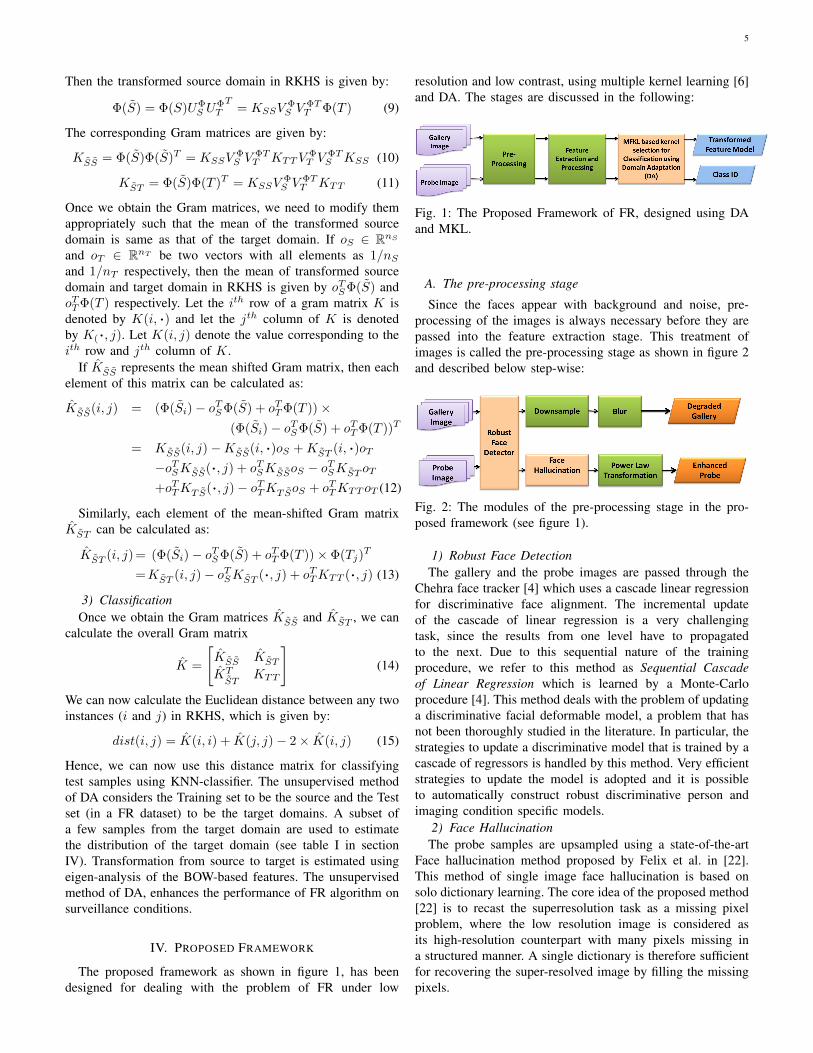
The proposed framework as shown in figure 1, has beendesigned for dealing with the problem of FR under low

resolution and low contrast, using multiple kernel learning [6]and DA. The stages are discussed in the following:

Fig. 1: The Proposed Framework of FR, designed using DAand MKL.

A. The pre-processing stage

Since the faces appear with background and noise, pre-processing of the images is always necessary before they arepassed into the feature extraction stage. This treatment ofimages is called the pre-processing stage as shown in figure 2and described below step-wise:

Fig. 2: The modules of the pre-processing stage in the pro-posed framework (see figure 1).

1) Robust Face DetectionThe gallery and the probe images are passed through the

Chehra face tracker [4] which uses a cascade linear regressionfor discriminative face alignment. The incremental updateof the cascade of linear regression is a very challengingtask, since the results from one level have to propagatedto the next. Due to this sequential nature of the trainingprocedure, we refer to this method as Sequential Cascadeof Linear Regression which is learned by a Monte-Carloprocedure [4]. This method deals with the problem of updatinga discriminative facial deformable model, a problem that hasnot been thoroughly studied in the literature. In particular, thestrategies to update a discriminative model that is trained by acascade of regressors is handled by this method. Very efficientstrategies to update the model is adopted and it is possibleto automatically construct robust discriminative person andimaging condition specific models.

2) Face HallucinationThe probe samples are upsampled using a state-of-the-art

Face hallucination method proposed by Felix et al. in [22].This method of single image face hallucination is based onsolo dictionary learning. The core idea of the proposed method[22] is to recast the superresolution task as a missing pixelproblem, where the low resolution image is considered asits high-resolution counterpart with many pixels missing ina structured manner. A single dictionary is therefore sufficientfor recovering the super-resolved image by filling the missingpixels.

6

3) Degradation of Gallery samplesThe gallery samples are downsampled by two using simple

bicubic interpolation method [18]. The gallery samples arethen blurred using an estimated Gaussian blur, σ. The σ isestimated using KL-Divergence [17], between the distributionsof the downsampled gallery and the upsampled probe images.The distribution of the target domain is estimated using threesamples per class but with no class labels (hence this isunsupervised). The graphs in figure 3 (a), (b) and (c) show theplots of KL-divergence with increasing values of Gaussian blurkernel, σ, for the three different datasets, FR SURV, SCfaceand ChokePoint, respectively. The optimal σopt is obtained at1.75, 1.7 and 1.2 for the three datasets and are recorded intable I. The gallery samples are degraded using this uniformblur σopt to obtain a degraded gallery.

Fig. 3: Plot of KL-Divergence between degraded gallery andprobe images with different values of σ used for degradation,in case of (a) FR SURV [33], (b) SCface [20] and (c)ChokePoint [44] datasets. The optimal values of σ are obtainedas: (a) 1.75, (b) 1.7 and (c) 1.2, respectively for the threedatasets.

TABLE I: Number of probe samples (per subject) used forestimation of σopt and in DA, for three datasets. Class (subjectID) information was made unavailable in both cases (as themethod is unsupervised). Only for the estimation of σopt, theentire gallery is used.

Dataset No. of samples used, for Values of σoptEstimation of σopt DASCface 5 3 1.7[20] for 30 subjects

FR SURV 5 3 1.75[33] for 20 subjectsChokePoint 5 6 1.2[44] for 20 subjects

4) Power Law TransformationTo cope with the contrast degradation, we perform Power

Law transformation [14] for contrast stretching the probeimages. The transformation function used is:

P (i, j) = k.C(i, j)γ (16)

where, P (i, j) and C(i, j) denotes the gray-level pixel valuesof the input and output image. We use γ = 1.25, k = 1. Visualresults as shown in figure 4 depicts contrast enhancement ofthe image for varying values of γ. We set γ = 1.25 based onvisual observation (empirical).

Fig. 4: (a) Probe images of three subjects; (b) Outputs ofCHEHRA [4] process; Gamma-corrected (equation 16) imageswith (c) γ = 1.25; (d) γ = 1.5; (e) γ = 1.75; and (f) γ = 1.9,from (I) FR SURV [33], (II) SCFace [20] and (III) ChokePoint[44] datasets.

For probe samples, we use:

Probeupsampled = Probecrop ↑ v (17)

Probetransformed(i, j) = Probeupsampled(i, j)γ (18)

where, Probecrop denotes the cropped probe sample based onChehra [4], ↑ denotes upsampling of the image by a factorv mentioned to the right of it, Probecrop denotes upsampledimage and Probetransformed denotes the image that will beused for feature-extraction. The γ is the parameter for gamma-correction of the image based on Power Law transformationwhich is given by equation 16.

B. Feature Extraction

The feature extraction process in the proposed method isbased on the set of features extracted from the degraded galleryand the enhanced probe face images. The set of features usedin the methods proposed includes Local Binary Pattern (LBP),Eigen Faces, Fisher Faces, Gabor faces, Weber Faces, Bagof Words (BOW), Vector of Linearly Agregated Descriptorsencoding based on Scale Invariant Feature Transform (VLAD-SIFT) [3], Fisher Vector encoding based on SIFT (FV-SIFT)[31].

1) Eigen FacesThis approach [40] of the detection and identification of

human faces and describe a working, near-real-time facerecognition system which tracks the face of a subject andthen recognizes the person by comparing characteristics ofthe face to those of known individuals. The approach treatsface recognition as a two-dimensional recognition problem,taking advantage of the fact that faces are normally uprightand thus may be described by a small set of 2-D characteristicviews. Face images are projected onto a feature space (facespace) that best encodes the variation among known faceimages. The face space is defined by the eigenfaces, which arethe eigenvectors of the set of faces; they do not necessarilycorrespond to isolated features such as eyes, ears, and noses.

2) Fisher FacesThis face recognition algorithm [9] is insensitive to large

variation in lighting direction and facial expression. Taking a

7

pattern classification approach, each pixel is considered in animage as a coordinate in a high-dimensional space. The imagesof a particular face, under varying illumination but fixed pose,lie in a 3D linear subspace of the high dimensional imagespace if the face is a Lambertian surface without shadowing.However, since faces are not truly Lambertian surfaces and doindeed produce self-shadowing, images will deviate from thislinear subspace. Rather than explicitly modeling this deviation,the image is projected into a subspace in a manner whichdiscounts those regions of the face with large deviation. Theprojection method is based on Fishers Linear Discriminantand produces well separated classes in a low-dimensionalsubspace, even under severe variation in lighting and facialexpressions.

3) Gabor FacesThe Gabor Feature Classifier (GFC) method [26] employs

an enhanced Fisher discrimination model on an augmentedGabor feature vector; which is derived from the Gabor wavelettransformation office images. For the three datasets used forexperimentation, table II gives the values of the parametersused, where v represents the different scales used, nµ is thenumber of orientations and µ is the orientation. Parameter σ,which determines the ratio of the Gaussian window width towavelength, is set to 2π, kmax is the wave-vector set to πand f the spatial frequency set to

√2. The Gabor wavelets,

whose kernels are similar to the 20 receptive field profilesof the mammalian cortical simple cells, exhibit desirablecharacteristics of spatial locality and orientation selectivity. Asa result, the Gabor transformed face images produce salientlocal and discriminating features that are suitable for facerecognition.

TABLE II: Parameters for experimenation in Gabor faces forthree datasets.

Datasets v nµ µFR SURV [33] {0, ..., 7} 8 {0, ..., 7}

SCFace [20] {0, ..., 5} 16 {0, ..., 15}ChokePoint [44] {0, ..., 4} 4 {0, ..., 3}

4) Weber FacesWebers law suggests that for a stimulus, the ratio be-

tween the smallest perceptual change and the backgroundis a constant, which implies stimuli are perceived not inabsolute terms but in relative terms. Inspired from this, anovel illumination insensitive representation of face imagesis exploited and analyzed under varying illuminations via aratio image, called Weber-face, [42] where a ratio betweenlocal intensity variation and the background is computed.

5) Local Binary PatternLocal binary patterns (LBP) [1] is a type of feature used for

classification in computer vision. LBP is the particular case ofthe Texture Spectrum model proposed in 1990. The face imageis divided into several regions from which the LBP featuredistributions are extracted and concatenated into an enhancedfeature vector to be used as a face descriptor. The procedureconsists of using the texture descriptor to build several local

descriptions of the face and combining them into a globaldescription. The operator assigns a label to every pixel of animage by thresholding the 3X3-neighborhood of each pixelwith the center pixel value and considering the result as abinary number. Then, the histogram of the labels can be usedas a texture descriptor.

6) Bag-of-Words (BOW)The feature extraction method proposed here is based on

the BOW [16] based on Dense-SIFT features. The dense-SIFTfeatures are calculated with a single-pixel shift of the windowover the face. The words used in processing are local imagefeatures. They may be constructed around interest points suchas scale-space extrema (e.g. SIFT keypoints [28]), or simplyon windows extracted from the image at regular positions andvarious scales. The features can be image patches, histogramsof gradient orientations or color histograms. As these featuresare sensitive to noise and are represented in high dimensionspaces, they are not directly used as words, but are categorizedusing a vector quantization technique such as k-means. Theoutput of this discretization is the dictionary.

7) Fisher Vector Encoding on dense-SIFT features (FV-SIFT)

This encoding [31] serves a similar purposes: summarizingin a vectorial statistic a number of local feature descriptors(e.g. SIFT [28]). Similarly to bag of visual words, they assignlocal descriptor to elements in a visual dictionary, obtainedwith a Gaussian Mixture Models for Fisher Vectors. However,rather than storing visual word occurrences only, the represen-tation stores a statistics of the difference between dictionaryelements and pooled local features. The Fisher encoding usesGMM to construct a visual word dictionary.

8) VLAD encoding on dense-SIFT features (VLAD-SIFT)The Vector of Linearly Agregated Descriptors [3] is similar

to Fisher vectors, but (i) it does not store second-orderinformation about the features and (ii) it typically use KMeansinstead of GMMs to generate the feature vocabulary (althoughthe latter is also an option). VLAD is constructed as follows:regions are extracted from an image using an affine invariantdetector, and described using the 128 dimensional SIFT de-scriptor. Each descriptor is then assigned to the closest clusterof a vocabulary of size k (where, k is typically 64 or 256, sothat clusters are quite coarse). For each of the k clusters, theresiduals (vector differences between descriptors and clustercenters) are accumulated, and the k - 128 dimensional sumsof residuals are concatenated into a single k×128 dimensionaldescriptor.

C. Kernel Selection by Multiple Kernel Learning

In support vector machine (SVM), selecting the kernel func-tion and its parameters are important issues during training.Generally, to select the best performing kernel among the setof kernel function (like Linear, RBF, etc.), a cross validationprocedure is used. In recent years, several MKL techniqueshave been proposed, where instead of selecting one specifickernel function and its corresponding parameters, multiplekernels are learned. MKL has two main advantages: (a)Different kernels correspond to different notions of similarity

8

Fig. 5: The Training Phase after pre-processing (see figure 2),to generate transformed features in RKHS for classification.

and instead of finding which works best, a MKL learningmethod helps to pick the best kernel or a combination ofkernels; and (b) Different kernels may use inputs coming fromdifferent representations, possibly from different sources. Insuch cases, combining kernels is one possible way to combinesources of multiple information. The training phase (see figure5) is described in section IV-D.

In this paper, we introduce a novel technique based onMKL, termed MFKL (Multi-feature Kernel Learning), forselecting the optimal feature-kernel combination for classifica-tion. The MFKL method determines the optimal weights forthe different kernels used for each feature category. All thefeatures are extracted individually from each of the galleryface images and passed into the MFKL module for optimalkernel selection for each feature. The ordered pair of thefeature and kernel < F iH ,Ki > is selected and stored forfurther processing. We assume that we have p features andtheir corresponding feature space be represented by X f , wheref ∈ {1, .., p}. Data points (xfi , yi) are given, where xfi ∈ X frepresents a feature vector in a particular feature space X f ,and yi ∈ {−1, 1}, ∀i ∈ 1, ..., n, are the class-labels. Foreach feature space X f , the choice is one out of m kernelsKfj ∈ Rn×n.We consider X =

⋃pf=1 X f and X ∈ Rl, where l =

l1+...+lp, such that xfi ∈ Rlf , where lf is the dimensionalityof the feature vector f . This problem follows a similar for-mulation as described in the classification algorithm, ”supportkernel machine”, as proposed by Bach et al. [6], and alsodiscussed in section III-B.

The primal problem is given by equation 2 and its dual byequation 3, with the same KKT conditions as mentioned insection III-B. In RKHS, we assume the embeddings of the datapoints xi in each feature space via a mapping φ : X f → Rc.We also assume that φ(x) has m distinct block componentsφ(x) = (φ1(x), ..., φm(x)). Following the usual recipe forkernel methods, we assume that this embedding is performedimplicitly, by specifying the inner product in Rc using a kernelfunction, which in this case is the sum of individual kernelfunctions on each block (subspace) component:

kf (xfi , xfj ) = φ(xfi )Tφ(xfj ) =

m∑s=1

φs(xfi )Tφs(x

fj )

=

m∑s=1

ks(xfi , x

fj )

(19)

Now, in the feature space, X , we have

k(xi, xj) =

p∑f=1

βfkf (xfi , xfj ) (20)

We now kernelize the problem described in equation 2 usingthis kernel function. In particular, we consider the dual of theproblem in equation 2 and substitute the kernel function forthe inner products in the equation 3 with the constraint ina particular feature space, rather than over the whole space,as (αTD(y)Kf

j D(y)α)12 ≤ djγ,∀j, f , where Kf

j is the j-th Gram matrix of the points {xfi } corresponding to the j-th kernel, for the f -th feature formed using k(xi, xj). Theseconstraints are derived from equations 3 and 5, which leadto the simultaneous selection of feature and its correspondingnon-zero kernels, based on the objective function (similar toequation 6), formulated as:

min maxj1

2d2j

αTD(y)Kfj D(y)α− αT e

w.r.t. α ∈ Rn

s.t. 0 ≤ α ≤ C,αT y = 0

(21)

Since the sparsity of the weights of the kernels is en-sured by KKT conditions, the non-zero kernels are usedfor classification in the testing phase. Let Jfj (α) denote

12d2j

αTD(y)Kfj D(y)α− αT e (see equation 21) and Jf (α) =

maxjJfj (α). Minimization of Jf (α) now reduces to an convex

optimization problem, as Jf (α) is also a non-differentiableconvex function subject to linear constraints. Our global ob-jective function is J(α) =

⋃pf=1 Jf (α). Union of convex

functions is not necessarily convex. Hence, a subgradientmethod [23] is used to solve each of these convex optimizationsub-problems, Jf (α), and finally the union of these are usedto obtain a global solution. Sparse solutions ensure that mostof the kernel weights are negligible (go near to zero) and avery few non-zero kernel weights remain for each feature.

In the proposed work, we take into account a set of kernelfunctions for the MKL method. The set of kernels consistsof Linear, Polynomial, Gaussian, RBF, Chi-square and RBF+ Chi-square. The equations of each of these kernels aretabulated in Table III.

TABLE III: Different types of kernel used in the MFKL, withtheir formulae.

Type of Kernel FormulaLinear k(x, y) = xT y + c

Polynomial k(x, y) = (αxT y + c)d

Gaussian k(x, y) = exp(−‖x−y‖

2

2σ2

)RBF k(x, y) = exp

(−‖x−y‖2σ2

)Chi-square k(x, y) = 1− Σni=1

(xi−yi)212 (xi+yi)

RBF + Chi-square k(x, y) = 1− Σni=1(xi−yi)212 (xi+yi)

+exp(−‖x−y‖2σ2

)

9

D. The Training Phase

In this phase of our proposed framework as shown in figure5, we have a set of feature F and a set of kernels K pairings.

F ={LBP,EigenFaces, F isherFaces,Gaborfaces,WeberFaces, V LAD − SIFT, FV − SIFT,BOW}

(22)

where each Fi ∈ F is the feature extracted from a face image;and

K ={Linear, Polynomial,Gaussian,RBF,Chi− square,RBF + Chi− square}

(23)

where each Ki ∈ K is a kernel function for the projection inthe RKHS, Hi.

The combination of F and K is passed into the MKLmodule to obtain the set of optimized pair of {Fj ,Kj}using the kernel selection method described in section IV-C.Based on the best feature-kernel pair obtained, the featurevector is projected into a higher dimensional space of RKHS.The training in DA is performed to obtain the final modelparameters along with the feature-kernel pairs. The number ofprobe samples used as targets for DA is mentioned in the tableI.

E. Classification based on K-Nearest Neighbor Classifier

In the testing phase as shown in figure 6, a query low-resolution face image is first pre-processed based on the pre-processing techniques described in section IV-A. Features areextracted from the pre-processed probe and passed into the DAmodule (RKHS), as shown in figure 6. The process of kernelselection corresponding to a feature is based on the MFKLtechnique proposed in the kernel selection stage. The overallgram matrix is created for each of these features. A majorityvoting is used based on the Nearest neighbor classification forthe probe samples. The winning class ID is selected as thebest match.

Fig. 6: The Testing phase in the proposed method (see figure1).

V. DETAILS OF SURVEILLANCE FACE DATABASES USED

For the experimentation purpose we have used three real-world surveillance face datasets, which are discussed below.In all three real-world datasets the gallery samples are takenin laboratory conditions, while for probes two out of the threedatasets are shot indoor, while one is shot outdoor.

A. FR SURV [33]FR SURV is a challenging database for FR, because the

gallery and the probe images are taken at different resolutionswith two different cameras. The gallery samples, taken indoorwith high resolution camera, have a resolution of 250 × 250pixels, while the probe samples, taken by surveillance camera,have a very low resolution of 45×45 pixels. The probe samplesare taken at a distance of 50-100 meters outdoor. Using Chehra[4] on both the gallery and probe samples, we produce croppedface regions at an average of 150X150 pixels and 33 × 33pixels respectively. The database consists 51 subjects with 20samples per class. Figure 7 shows two samples of the galleryimages and the their respective probe image (cropped usingChehra [4]).

Fig. 7: Samples of two subjects from FR SURV Database[33]: (I) (a), (c) Gallery images; and (I) (b), (d) correspondingProbe images; (II) (a)-(d) Cropped faces from (I) using Chehra[4].

B. SCFace [20]SCface is also a challenging database for FR as the images

were taken at different surveillance conditions. The databasehas a huge collection of static images of 130 different people.Images were captured by five different video surveillancecameras (cam1, cam2, cam3, cam4, cam5). Two cameras werealso used in the night vision mode (cam6 and cam7). Allthese images were collected indoor with varying quality andresolution levels at three different distances. The training setconsists of nine images: one frontal and four each in leftand right rotations. The dataset has an image taken froman infra-red camera(cam8). Figure 8 shows the images for asingle person in the dataset. The gallery has images of size2048×3072 pixels which are cropped by VJFD to an averageof 800× 600 pixels. The probe images at Distance 1,2 and 3has a resolution of 75× 100, 108× 144 and 168× 224 pixelsrespectively which are cropped by Chehra [4] to an averageof 40× 40, 60× 60 and 100× 100 pixels respectively. We donot use the cam6 and cam7 as they are IR images.

C. ChokePoint [44]Wong et al. [44] collected a new video dataset, termed

ChokePoint, designed for experiments in person identifica-

10

Fig. 8: SCface Database [20]: (I) Gallery images; ProbeImages at (II) Distance 1; (III) Distance 2; and (IV) Distance3; Right column shows the Chehra [4] output for any one ofthe samples in each row.

tion/verification under real-world surveillance conditions usingexisting technologies. An array of three cameras was placedabove several portals (natural choke points in terms of pedes-trian traffic) to capture subjects walking through each portalin a natural way (see figures 9 and 10).

Fig. 9: An example of the recording setup used for theChokePoint dataset [44]. A camera rig contains 3 camerasplaced just above a door, used for simultaneously recordingthe entry of a person from 3 viewpoints. The variationsbetween viewpoints allow for variations in walking directions,facilitating the capture of a near-frontal face by one of thecameras.

Fig. 10: Example shots from the ChokePoint dataset [44],showing portals with various backgrounds.

The dataset consists of 25 subjects (19 male and 6 female)in portal 1 and 29 subjects (23 male and 6 female) in portal2. In total, it consists of 48 video sequences and 64,204 face

images. Each sequence was named according to the recordingconditions (eg. P2E S1 C3) where P, S, and C stand for portal,sequence and camera, respectively. E and L indicate subjectseither entering or leaving the portal. The numbers indicate therespective portal, sequence and camera label. For example,P2L S1 C3 indicates that the recording was done in Portal 2,with people leaving the portal, and captured by camera 3 in thefirst recorded sequence. The ChokePoint dataset does not havevariation in resolution. But the difference lies in the differentcameras used for capturing the image due to different cameraparameters and the illumination variations. This feature makesit suitable to be tackled with DA.

For experimentation, we consider the images obtained fromcamera, C1 as the Gallery set, since it contains maximumfrontal images with better lighting conditions. The othercameras are considered as probe images. We do not considerthe sequence S5, as it contains crowded scenario. Since theimages obtained from C1 are crisp and have better illumi-nation conditions than C2 and C3, the gallery and probe ispassed through all the pre-processing stages, except the facehallucination stage, as the resolution of the images obtainedfrom all these cameras are similar.

D. Intermediate results of face processing

The face images go through the several stages of pre-processing, as described in section IV-A. An example toillustrate the pre-processing stages is shown in figure 11, forthe SCFace [20] dataset. The top row illustrates the effect ofpre-processing on the gallery images, while the bottom rowillustrates the effect of pre-processing on the probe images.Figure 11(a) shows the original images available in the dataset,while figure 11(b) shows the landmark points detected by theChehra [4] on the face images. Based on these landmarkpoints, we obtain a tightly cropped face image as shown infigure 11(c). Figure 11(d) shows the result of downsamplingof the gallery images and upsampling of the probe imagesby Face Hallucination technique, as discussed in sectionIV-A2. The downsampled gallery images are blurred using aGaussian kernel to obtain the degraded gallery images whilethe upsampled probe images are passed through Power lawtransformation to obtain moderately enhanced probe imagesas shown in figure 11(e). Face hallucination is not appliedon the probe samples in the ChokePoint [44] dataset, as theresolution of the gallery and probe samples are similar in thedataset.

Figure 12 shows the examples of the degraded gallery (inthe top row) and the enhanced probe (in the bottom row)images of a single subject from the three surveillance datasets,used in our experimentation. These degraded gallery and theenhanced probe images are used for feature extraction. Theoriginal gallery and probes are also shown with similar spatialresolution to illustrate the efficiency of the pre-processingstage (ignore resolution which is different).

VI. EXPERIMENTAL RESULTS

Rigorous experimentation is carried on three real-worlddatasets; SCface [20], FR SURV [33], and ChokePoint [44]

11

Fig. 11: Pre-processing stages on SCFace [20] for a subject:(a) Original image, (b) Landmarks detected by Chehra [4], (c)the cropped faces obtained using Chehra, (d) Downsampledimage of gallery and upsampled image of probe, (e) Finaldegraded gallery and enhanced probe images.

Fig. 12: Example shots from the three datasets (one sampleeach), showing the degraded gallery and the enhanced probeimages on the cropped faces produced by Chehra [4]

The proposed methods are compared with several other recentstate-of-the-art methods and the results are reported in tableIV using Rank-1 Recognition Rate.

TABLE IV: Rank-1 Recognition Rate for different methods.Results in bold, exhibit the best performance.

Sl. Algorithm SCface FR SURV ChokePoint[20] [33] [44]

1 EDA1 [8] 47.65 7.82 54.212 COMP DEG

[33]4.32 43.14 62.59

3 MDS [10] 42.26 12.06 52.134 KDA1 [8] 35.04 38.24 56.255 Gopalan [19] 2.06 2.06 58.626 Kliep [39] 37.51 28.79 63.287 Naive 75.27 45.78 65.768 Proposed

Method78.31 55.23 84.62

In case of Naive combination, the source and the targetdomain samples are used without transformation for trainingand domain samples are used as probes. In EDA1 method,proposed by Banerjee et al. [8], DA processing based onan eigenvector based transformation, whose extension in theRKHS is termed as KDA1. Rudrani et al. [33] (COMP DEG)tries to bridge the gap between the gallery and the probesamples by projecting them both into a lower dimensionalsubspace determined by the principal components of the

feature vectors obtained from each face. This paper also acts asthe source for the dataset, FR SURV [33]. Multi-dimensionalscaling (MDS) proposed by Biswas et al. in [10] projects boththe gallery and the probe samples into a common subspacefor classification. The methods proposed by Gopalan et al.[19] and Kliep [39] are two DA based techniques used forobject classification accross domains. We can observe that themethod proposed in this paper have outperformed (our resultsare given in bold, in Table IV) all the other competing methodsby a considerable margin. The complexity of the datasets isalso observed by the results of FR, which are all moderatelylow in many cases.

Results are also reported using ROC (for identification) andCMC (for verification) measures, as shown in figures 13 - 15,for the three datasets respectively. The plot drawn in red showthe performance of our proposed method. We can observe thatthe red curves in all the plots outperform all other competingmethods. On an average, the second best performance is givenby the naive approach since the MFKL is also incorporatedinto it, while the method proposed by Gopalan et al. [19]performs generally the worst.

Fig. 13: (a) ROC and (b) CMC plots for performance analysisof different methods, using SCFace [20] dataset.

Fig. 14: (a) ROC and (b) CMC plots for performance analysisof different methods, using FR SURV [33] dataset.

As we look closer into the the table IV row-wise, wecan easily observe that the FR SURV datasets has the leastaccuracy. This is an indication that there is still further scopeof improvement in this field. Also, it shows that the database isquite tough to handle. As we can see that the gallery samples inFR SURV are all taken in Indoor laboratory conditions and theprobe samples are taken in Outdoor conditions which resultsin the large complexity of the database. Since FR SURV isan outdoor dataset, we can see the accuracy of FR is less thanthat of the ChokePoint dataset, which is the easiest to handleamong the three. The SCface and the ChokePoint datasets are

12

Fig. 15: (a) ROC and (b) CMC plots for performance analysisof different methods, using ChokePoint [44] dataset.

two indoor surveillance datasets. Experiments are done in bothidentification and verification mode. There is still scope ofimprovement to find a more effective effective transformationsuch that the distribution of the features of the gallery andthe probe become similar. The other two datasets have boththe gallery and the probe taken in Indoor scenario. The effec-tiveness of the DA used in this paper is clearly visible in theresults of EDA1 and KDA1. The non-linear transformations inKDA1 proves to be more effective which motivates this paperto concentrate mostly on the DA in RKHS. The effectivenessof the MKL based method is evident when we try to focuson the Naive combination results. It is very competitive inall the three datasets. The Naive combination is the completeFramework without the DA module, incorporating also theMKL process. When these two powerful tools are combined,our proposed method outperforms all other methods by aconsiderable margin.

VII. CONCLUSION

An efficient method to tackle the problem of low-contrastand low-resolution in face recognition under surveillance sce-nario is proposed in this paper. The method proposes a novelkernel selection method using MFKL to obtain an optimalpairing of feature and kernel for eigen-domain transformationbased unsupervised DA in the RKHS. The three metrics usedto compare the performance of our proposed method withthe recent state-of-the-art techniques, show a great deal ofsuperiority of our method than the other techniques, usingthree real-world surveillance face datasets.

REFERENCES

[1] T. Ahonen, A. Hadid, and M. Pietikainen. Face description with localbinary patterns: Application to face recognition. IEEE Transactions onPattern Analysis and Machine Intelligence, 28(12):2037–2041, 2006.

[2] R. Alain, R. Francis, C. Phane, and S. Yves. Simple mkl. Journal ofMachine Learning Research, 9:2491–2521, 2008.

[3] R. Arandjelovic and A. Zisserman. All about vlad. In Proceedings of theIEEE Conference on Computer Vision and Pattern Recognition, pages1578–1585, 2013.

[4] A. Asthana, S. Zafeiriou, S. Cheng, and M. Pantic. Incremental facealignment in the wild. In Proceedings of the IEEE Conference onComputer Vision and Pattern Recognition, 2014.

[5] Y. Aytar and A. Zisserman. Tabula rasa: Model transfer for objectcategory detection. In IEEE International Conference on ComputerVision, pages 2252–2259. IEEE, 2011.

[6] F. R. Bach, G. R. Lanckriet, and M. I. Jordan. Multiple kernel learning,conic duality, and the smo algorithm. In Proceedings of the twenty-firstinternational conference on Machine learning, page 6. ACM, 2004.

[7] M. Baktashmotlagh, M. T. Harandi, B. C. Lovell, and M. Salzmann.Unsupervised domain adaptation by domain invariant projection. InInternational Conference on Computer Vision, pages 769–776. IEEE,2013.

[8] S. Banerjee, S. Samanta, and S. Das. Face recognition in surveillanceconditions with bag-of-words, using unsupervised domain adaptation.In Proceedings of Indian Conference on Computer Vision Graphics andImage Processing, page 50. ACM, 2014.

[9] P. N. Belhumeur, J. P. Hespanha, and D. J. Kriegman. Eigenfaces vs.fisherfaces: Recognition using class specific linear projection. IEEETransactions on Pattern Analysis and Machine Intelligence, 19(7):711–720, 1997.

[10] S. Biswas, K. W. Bowyer, and P. J. Flynn. Multidimensional scalingfor matching low-resolution face images. IEEE Transactions on PatternAnalysis and Machine Intelligence, 34(10):2019–2030, 2012.

[11] W. Dai, G.-R. Xue, Q. Yang, and Y. Yu. Transferring naive bayesclassifiers for text classification. In Proceedings of the national con-ference on artificial intelligence, volume 22, page 540. Menlo Park,CA; Cambridge, MA; London; AAAI Press; MIT Press; 1999, 2007.

[12] L. Duan, D. Xu, and I. W. Tsang. Domain adaptation from multiplesources: A domain-dependent regularization approach. IEEE Transac-tions on Neural Networks and Learning Systems, 23(3):504–518, 2012.

[13] H. Dym. J contractive matrix functions, reproducing kernel Hilbertspaces and interpolation, volume 71. American Mathematical Soc.,1989.

[14] H. Farid. Blind inverse gamma correction. IEEE Transactions on ImageProcessing, 10(10):1428–1433, 2001.

[15] B. Fernando, A. Habrard, M. Sebban, and T. Tuytelaars. Unsupervisedvisual domain adaptation using subspace alignment. In InternationalConference on Computer Vision, pages 2960–2967. IEEE, 2013.

[16] D. Filliat. A visual bag of words method for interactive qualitativelocalization and mapping. In IEEE International Conference on Roboticsand Automation, pages 3921–3926. IEEE, 2007.

[17] J. Goldberger, S. Gordon, and H. Greenspan. An efficient imagesimilarity measure based on approximations of kl-divergence betweentwo gaussian mixtures. In Internation Conference on Computer Vision,pages 487–493. IEEE, 2003.

[18] R. C. Gonzalez and R. E. Woods. Digital Image Processing. Addison-Wesley, Reading, MA, 1992.

[19] R. Gopalan, R. Li, and R. Chellappa. Domain adaptation for objectrecognition: An unsupervised approach. In Internation Conference onComputer Vision, pages 999–1006, 2011.

[20] M. Grgic, K. Delac, and S. Grgic. Scface–surveillance cameras facedatabase. Multimedia tools and applications, 51(3):863–879, 2011.

[21] J. Jiang and C. Zhai. Instance weighting for domain adaptation in nlp. InAssociation for Computer Linguistics, volume 7, pages 264–271, 2007.

[22] F. Juefei-Xu and M. Savvides. Single face image super-resolution viasolo dictionary learning. In IEEE International Conference on ImageProcessing (ICIP), volume 2, 2015.

[23] S. Kim and H. Ahn. Convergence of a generalized subgradient methodfor nondifferentiable convex optimization. Mathematical Programming,50(1-3):75–80, 1991.

[24] G. R. Lanckriet, N. Cristianini, P. Bartlett, L. E. Ghaoui, and M. I.Jordan. Learning the kernel matrix with semidefinite programming. TheJournal of Machine Learning Research, 5:27–72, 2004.

[25] G. R. Lanckriet, T. De Bie, N. Cristianini, M. I. Jordan, and W. S.Noble. A statistical framework for genomic data fusion. Bioinformatics,20(16):2626–2635, 2004.

[26] C. Liu and H. Wechsler. Gabor feature based classification using theenhanced fisher linear discriminant model for face recognition. IEEETransactions on Image processing, 11(4):467–476, 2002.

[27] M. S. Lobo, L. Vandenberghe, S. Boyd, and H. Lebret. Applications ofsecond-order cone programming. Linear algebra and its applications,284(1):193–228, 1998.

[28] D. G. Lowe. Distinctive image features from scale-invariant keypoints.International Journal of Computer Vision, 60(2):91–110, 2004.

[29] S. J. Pan, I. W. Tsang, J. T. Kwok, and Q. Yang. Domain adaptation viatransfer component analysis. IEEE Transactions on Neural Networks,22(2):199–210, 2011.

[30] M. A. Pathak and E. H. Nyberg. Learning algorithms for domainadaptation. In Advances in Machine Learning, pages 293–307. Springer,2009.

[31] F. Perronnin, J. Sanchez, and T. Mensink. Improving the fisher kernel forlarge-scale image classification. In European Conference on ComputerVision, pages 143–156. Springer, 2010.

13

[32] C.-X. Ren, D.-Q. Dai, and H. Yan. Coupled kernel embedding forlow-resolution face image recognition. IEEE Transactions on ImageProcessing, 21(8):3770–3783, 2012.

[33] S. Rudrani and S. Das. Face recognition on low quality surveillanceimages, by compensating degradation. In ICIAR, pages 212–221. LNCS,Springer, 2011.

[34] S. Samanta and S. Das. Unsupervised domain adaptation using eigen-analysis in kernel space for categorisation tasks. Image Processing, IET,9(11):925–930, 2015.

[35] S. Samanta, T. Selvan, and S. Das. Modeling sequential domain shiftthrough estimation of optimal sub-spaces for categorization. In BritishMachine Vision Conference, 2014.

[36] A. Shrivastava, V. M. Patel, and R. Chellappa. Multiple kernel learningfor sparse representation-based classification. IEEE Transactions onImage Processing, 23(7):3013–3024, 2014.

[37] S. Sonnenburg, G. Ratsch, C. Schafer, and B. Scholkopf. Large scalemultiple kernel learning. The Journal of Machine Learning Research,7:1531–1565, 2006.

[38] M. Sugiyama, S. Nakajima, H. Kashima, P. V. Buenau, and M. Kawan-abe. Direct importance estimation with model selection and its appli-cation to covariate shift adaptation. In Advances in neural informationprocessing systems, pages 1433–1440, 2008.

[39] M. Sugiyama, S. Nakajima, H. Kashima, P. von Bunau, and M. Kawan-abe. Direct importance estimation with model selection and its appli-cation to covariate shift adaptation. In Neural Information ProcessingSystems, pages 1962–1965, 2007.

[40] M. Turk and A. Pentland. Eigenfaces for recognition. Journal ofcognitive neuroscience, 3(1):71–86, 1991.

[41] P. Viola and M. J. Jones. Robust real-time face detection. InternationalJournal of Computer Vision, 57(2):137–154, 2004.

[42] B. Wang, W. Li, W. Yang, and Q. Liao. Illumination normalization basedon weber’s law with application to face recognition. Signal ProcessingLetters, IEEE, 18(8):462–465, 2011.

[43] C. Wang and S. Mahadevan. Heterogeneous domain adaptation usingmanifold alignment. In IJCAI Proceedings-International Joint Confer-ence on Artificial Intelligence, volume 22, page 1541, 2011.

[44] Y. Wong, S. Chen, S. Mau, C. Sanderson, and B. C. Lovell. Patch-basedprobabilistic image quality assessment for face selection and improvedvideo-based face recognition. In IEEE Biometrics Workshop, ComputerVision and Pattern Recognition (CVPR) Workshops, pages 81–88. IEEE,June 2011.

[45] Z. Xu, R. Jin, H. Yang, I. King, and M. R. Lyu. Simple and efficientmultiple kernel learning by group lasso. In Proceedings of the 27thinternational conference on machine learning (ICML-10), pages 1175–1182, 2010.

[46] J. Yang, R. Yan, and A. G. Hauptmann. Cross-domain video conceptdetection using adaptive svms. In Proceedings of the 15th internationalconference on Multimedia, pages 188–197. ACM, 2007.

[47] K. C. Yow and R. Cipolla. Feature-based human face detection. Imageand vision computing, 15(9):713–735, 1997.

[48] X. Zhu and D. Ramanan. Face detection, pose estimation, and landmarklocalization in the wild. In Proceedings of the IEEE Conference onComputer Vision and Pattern Recognition, pages 2879–2886. IEEE,2012.

[49] W. W. Zou and P. C. Yuen. Very low resolution face recognition problem.IEEE Transactions on Image Processing, 21(1):327–340, 2012.