k-adaptive partitioning for survival data
TRANSCRIPT

Introduction Proposed method Simulation studies Real example Conclusion References
K-Adaptive Partitioning for Survival Data
with an Application to SEER
Soo-Heang Eo
with Sungwan Bang, Seung-Mo Hong, HyungJun Cho
Department of Statistics
Korea University
April 25, 2014

Introduction Proposed method Simulation studies Real example Conclusion References
Table of Contents
Introduction
Motivation example
Previous studies
Proposed method
Finding the best split set
Finding optimal number of subgroups
Simulation studies
Simulation design
Simulation results
Real example
Conclusion
References

Introduction Proposed method Simulation studies Real example Conclusion References
Cancer staging
cancer staging system that describes the extent of cancer in a
patient’s body. [2]

Introduction Proposed method Simulation studies Real example Conclusion References
TNM staging system
The TNM Classification of Malignant Tumors (TNM) is a cancer
staging system that describes the extent of cancer in a patient’s
body. [2]
T describes the size of the tumor and whether it has invaded
nearby tissue,
N describes distant metastasis lymph node (spread of
cancer from one body part to another).
M describes regional lymph nodes that are involved,

Introduction Proposed method Simulation studies Real example Conclusion References
Previous studies
• Hilsenbeck and Clark (1996) concerned simulation studies to
examine the effects of number of cutpoints and true marker
prognostic effect size [3].
• Contal and O’Quigley (1999) proposed the asymptotic distribution
of a re-scaled rank statistic [1].
• Lausen et al. (1994) and Hong et al. (2007) employed decision
tree methodology [8, 4].
• Hothorn and Lausen (2003) used maximally selected rank
statistics [6] to find the best cutpoints and extended to CTree [5].
• Ishwaran et al. (2009) adopted the idea of random survival forests
[7].
Most approaches to find cut-off point have been based on concepts from
binary split.
Introduction Proposed method Simulation studies Real example Conclusion References
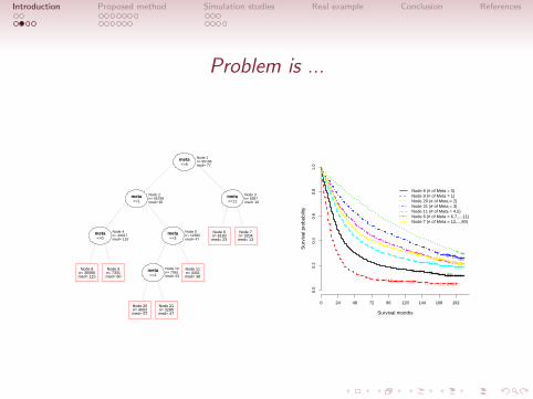
Problem is ...
|
Node 8 Node 9
Node 20 Node 21
Node 11
Node 6 Node 7
n= 36086 n= 7331
n= 4693 n= 3288
n= 4401
n= 6183 n= 3204
med= 115 med= 80
med= 57 med= 47
med= 38
med= 23 med= 13
meta
meta
meta meta
meta
meta
<=5
<=1
<=0 <=3
<=2
<=11
Node 1
Node 2
Node 4 Node 5
Node 10
Node 3
n= 65186
n= 55799
n= 43417 n= 12382
n= 7981
n= 9387
med= 77
med= 95
med= 110 med= 47
med= 53
med= 19
Survival months
Sur
viva
l pro
babi
lity
0.0
0.2
0.4
0.6
0.8
1.0
0 24 48 72 96 120 144 168 192
Node 8 (# of Meta = 0)Node 9 (# of Meta = 1)Node 20 (# of Meta = 2)Node 21 (# of Meta = 3)Node 11 (# of Meta = 4,5)Node 6 (# of Meta = 6,7,...,11)Node 7 (# of Meta = 12,...,80)
Introduction Proposed method Simulation studies Real example Conclusion References
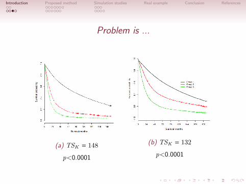
Problem is ...
(a) TSK = 148
p<0.0001
(b) TSK = 132
p<0.0001

Introduction Proposed method Simulation studies Real example Conclusion References
Our aim is to
• Divide the whole data D into K heterogeneous subgroups
D1, . . . ,DK based on the information of X .
• Overcome the limitation that some subgroups differ
substantially in survival, but others may differ barely or
insignificantly.
• Evaluate multi-way split points simultaneously and find an
optimal set of cutpoints.
• Implement the proposed algorithm into an R package kaps.

Introduction Proposed method Simulation studies Real example Conclusion References
Finding the best split set
Let Ti be a survival time, Ci a censoring status, and Xi be an
ordered covariate for the i th observation. We observe the triples
(Yi , δi ,Xi ) and define
Yi = min(Ti ,Ci ) and δi = I (Ti ≤ Ci ),
which represent the observed response variable and the censoring
indicator, respectively.

Introduction Proposed method Simulation studies Real example Conclusion References
Finding the best split set
Let χ21 be the χ2 statistic with one degree of freedom (df) for
comparing the g th and hth of K subgroups created by a split set
sK when K is given. For a split set sK of D into D1,D2, . . . ,DK ,
the test statistic for a measure of deviance can be defined as
T1(sK ) = min1≤g<h≤K
χ21 for sK ∈ SK , (1)
where SK is a collection of split sets sK generating K disjoint
subgroups.

Introduction Proposed method Simulation studies Real example Conclusion References
Finding the best split set
Then, take s∗K
as the best split set such that
T ∗1(s∗K ) = maxsK∈SK
T1(sK ). (2)
The best split s∗K
is a set of (K − 1) cutpoints which clearly
separate the data D into K disjoint subsets of the data:
D1,D2, . . . ,DK .

Introduction Proposed method Simulation studies Real example Conclusion References
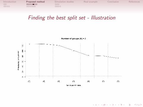
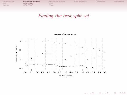
Finding the best split set - Illustration
• We assumed that the patients were divided into 3 heterogeneous
groups by the number of lymph nodes (X = {0, 1, . . . , 6}).
• Each group was categorised as D1,D2 and D3.
• 3 pairs of groups (D1vs .D2,D2vs .D3, and D1vs .D3).
• We imagined existing 3 cut-off points candidates, each of which
were composed of two cutpoints; {0,1}, {0,2}, and {1,2}.
• For example, the cutpoints candidate {0, 1} mean that
D1 = {X = 0},D2 = {0 < X ≤ 1}, and D3 = {X > 1}.
• Out of the 3 pairs of the candidates, the smallest test statistic was
selected as a representative statiatic for the candidate.
Introduction Proposed method Simulation studies Real example Conclusion References
Finding the best split set - Illustration
Introduction Proposed method Simulation studies Real example Conclusion References
Finding the best split set

Introduction Proposed method Simulation studies Real example Conclusion References
Algorithm 1. Finding the best split set for given K
Step 1: Compute chi-squared test statistics χ21 for all possible pairs, g and h, of K
subgroups by sK , where 1 ≤ g < h ≤ K and sK is a split set of (K − 1)
cutpoints generating K disjoint subgroups.
Step 2: Obtain the minimum pairwise statistic T1(sK ) by minimizing χ21 for all
possible pairs, i .e., T1(sK ) = min1≤g<h≤K χ21 for sK ∈ SK ,where SK is a
collection of split sets sK generating K disjoint subsets of the data.
Step 3: Repeat Steps 1 and 2 for all possible split sets SK .
Step 4: Take the best split set s∗K
such that T ∗1(s∗K
) = maxsK ∈SKT1(sK ). When two
or more split sets have the maximum T ∗1 of the minimum pairwise statistics,
choose the best split set with the largest overall statistic T ∗K−1
.

Introduction Proposed method Simulation studies Real example Conclusion References
Finding optimal subgroups
• One of the important issues is to determine a reasonable
number of subgroups, i.e. the selection of an optimal K .
• We find an optimal multi-way split at a time for the given
number of subgroups.
• We need to choose only one of a possible number of
subgroups.
• For a data-driven objective choice, we here suggest a
statistical procedure to choose an optimal number of
subgroups.
Introduction Proposed method Simulation studies Real example Conclusion References
Finding optimal subgroups
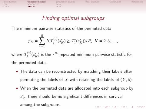
The minimum pairwise statistics of the permuted data
pK =
R∑r=1
I (T (r )1 (s∗K ) ≥ T ∗1(s∗K ))/R, K = 2, 3, . . . ,
where T(r )1 (s∗
K) is the r th repeated minimum pairwise statistic for
the permuted data.
• The data can be reconstructed by matching their labels after
permuting the labels of X with retaining the labels of (Y , δ).
• When the permuted data are allocated into each subgroup by
s∗K
, there should be no significant differences in survival
among the subgroups.

Introduction Proposed method Simulation studies Real example Conclusion References
Finding optimal subgroups
We choose the largest number to discover as many significantly
different subgroups as possible, given that the corrected p-values
are smaller than or equal to a pre-determined significance level
K = max{K |pcK ≤ α,K = 2, 3, . . .},
where pCK
is the corrected p-values for multiple comparison because
there are (K − 1) comparisons between two adjacent subgroups
Introduction Proposed method Simulation studies Real example Conclusion References
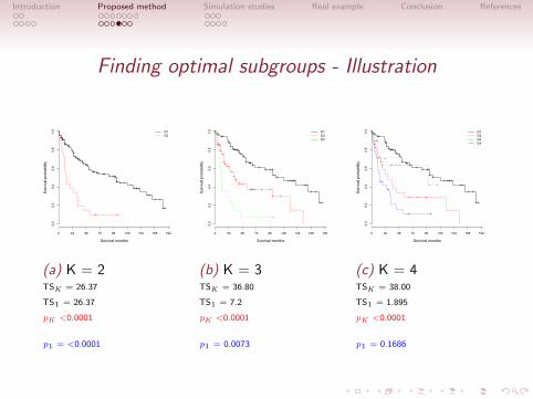
Finding optimal subgroups - Illustration
Survival months
Sur
viva
l pro
babi
lity
0.0
0.2
0.4
0.6
0.8
1.0
0 24 48 72 96 120 144 168 192
G1G2
(a) K = 2TSK = 26.37
TS1 = 26.37
pK <0.0001
p1 = <0.0001
Survival months
Sur
viva
l pro
babi
lity
0.0
0.2
0.4
0.6
0.8
1.0
0 24 48 72 96 120 144 168 192
G1G2G3
(b) K = 3TSK = 36.80
TS1 = 7.2
pK <0.0001
p1 = 0.0073
Survival months
Sur
viva
l pro
babi
lity
0.0
0.2
0.4
0.6
0.8
1.0
0 24 48 72 96 120 144 168 192
G1G2G3G4
(c) K = 4TSK = 38.00
TS1 = 1.895
pK <0.0001
p1 = 0.1686
Introduction Proposed method Simulation studies Real example Conclusion References
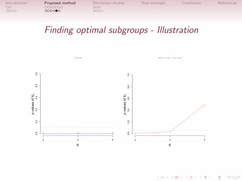
Finding optimal subgroups - Illustration
meta
Sur
viva
l mon
ths
0 10 20 30
1248
7296
120
144
168
192
Event
Censored
Survival months
Sur
viva
l pro
babi
lity
0.0
0.2
0.4
0.6
0.8
1.0
0 24 48 72 96 120 144 168 192
G1
G2
G3
K
p-va
lues
of X
k
2 3 4
0.0
0.1
0.2
0.3
0.4
0.5
K
p-va
lues
of X
1
2 3 4
0.0
0.2
0.4
0.6
0.8
1.0

Introduction Proposed method Simulation studies Real example Conclusion References
Algorithm 2. Selecting the optimal number of subgroups
Step 1: Find s∗K
and T1(s∗K
) with the raw data for each K using Algorithm 1.
Step 2: Construct the permuted data by permuting the labels of X whilst retaining
the labels of (Y , δ).
Step 3: Allocate the permuted data into each subgroup by s∗K
.
Step 4: Obtain the minimum pairwise statistic T(r )1 (s∗
K) for the permuted data.
Step 5: Repeat steps 2 to 4 R times, and then obtain
T(1)1 (s∗
K),T (2)
1 (s∗K
), . . . ,T (R)1 (s∗
K).
Step 6: Compute the permutation p-value pK for each K , i .e.,
pK =∑R
r=1 I (T (r )1 (s∗
K) ≥ T1(s∗
K))/R, K = 2, 3, . . . .
Step 7: Correct the permutation p-value pK by correcting for multiple comparisons,
e.g ., corrected p-value pcK= pK /(K − 1),K = 2, 3, . . ..
Step 8: Select the largest K when the corrected p-values are less than or equal to α,
i .e., K = max{K | pcK≤ α,K = 2, 3, . . .}.
Introduction Proposed method Simulation studies Real example Conclusion References
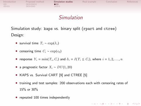
Simulation
Simulation study: kaps vs. binary split (rpart and ctree)
Design:
• survival time Ti ∼ exp(λi )
• censoring time Ci ∼ exp(c0)
• response Yi = min(Ti ,Ci ) and δi = I (Ti ≤ Ci ), where i = 1, 2, . . . ,n
• a prognostic factor Xi ∼ DU (1, 20)
• KAPS vs. Survival CART [9] and CTREE [5]
• training and test samples: 200 observations each with censoring rates of
15% or 30%
• repeated 100 times independently

Introduction Proposed method Simulation studies Real example Conclusion References
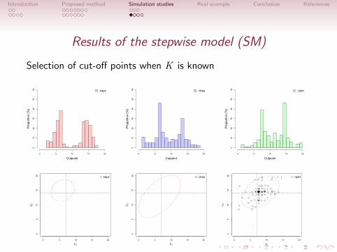
Setting 1 - stepwise model
We consider the following stepwise model (SM) defining parameter
λi as follows.
λi =
0.02, Xi ≤ 7,
0.04, 7 < Xi ≤ 14,
0.08, 14 < Xi ,
(3)
This model has three different hazard rates that are distinguished
by two cutpoints 7 and 14.

Introduction Proposed method Simulation studies Real example Conclusion References
Setting 2 - linear model
In addition, we consider the following linear model (LM) defining
parameter λi as follows.
λi = 0.1Xi . (4)
In this model, λi depends on Xi linearly.
It follows that Yi depends on Xi nonlinearly.
This model has a number of different hazard rates.
Introduction Proposed method Simulation studies Real example Conclusion References
Results of the stepwise model (SM)
Selection of cut-off points when K is known
Cutpoint
Pro
porti
on (%
)
0 5 10 15 20
010
2030
4050
60 kaps
Cutpoint
Pro
porti
on (%
)
0 5 10 15 20
010
2030
4050
60 ctree
Cutpoint
Pro
porti
on (%
)
0 5 10 15 20
010
2030
4050
60 rpart
0 5 10 15 20
05
1015
20
C1
C2
kaps
0 5 10 15 20
05
1015
20
C1
C2
ctree
0 5 10 15 20
05
1015
20
C1
C2
rpart
Introduction Proposed method Simulation studies Real example Conclusion References
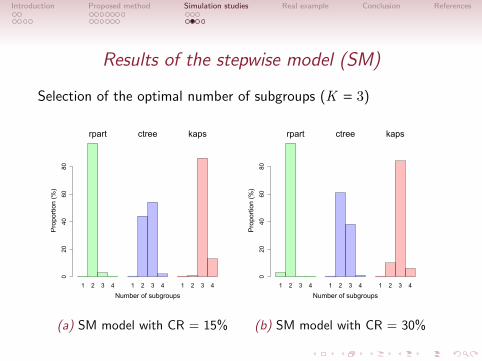
Results of the stepwise model (SM)
Selection of the optimal number of subgroups (K = 3)
Number of subgroups
Pro
porti
on (%
)0
2040
6080
1 2 3 4 1 2 3 4 1 2 3 4
rpart ctree kaps
(a) SM model with CR = 15%
Number of subgroups
Pro
porti
on (%
)0
2040
6080
1 2 3 4 1 2 3 4 1 2 3 4
rpart ctree kaps
(b) SM model with CR = 30%
Introduction Proposed method Simulation studies Real example Conclusion References
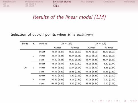
Results of the linear model (LM)
Selection of cut-off points when K is unknown
Model K Method CR = 15% CR = 30%
Overall Pairwise Overall Pairwise
rpart 43.57 (1.17) 43.57 (1.17) 38.73 (1.03) 38.73 (1.03)
2 ctree 38.94 (1.16) 38.94 (1.16) 36.29 (1.01) 36.29 (1.01)
kaps 44.52 (1.15) 44.52 (1.15) 38.74 (1.11) 38.74 (1.11)
rpart 48.07 (1.47) 6.87 (0.50) 43.21 (1.11) 6.32 (0.44)
LM 3 ctree 55.64 (1.39) 12.94 (1.14) 47.99 (1.40) 8.33 (0.64)
kaps 54.96 (1.39) 13.83 (0.63) 47.95 (1.36) 11.33 (0.59)
rpart 59.60 (1.59) 2.59 (0.26) 53.01 (1.33) 2.30 (0.22)
4 ctree 59.82 (1.35) 3.17 (0.37) 52.05 (1.34) 2.10 (0.21)
kaps 61.27 (1.39) 3.22 (0.24) 53.48 (1.34) 2.70 (0.23)
Introduction Proposed method Simulation studies Real example Conclusion References
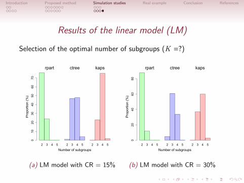
Results of the linear model (LM)
Selection of the optimal number of subgroups (K =?)
Number of subgroups
Pro
porti
on (%
)0
1020
3040
5060
70
2 3 4 5 2 3 4 5 2 3 4 5
rpart ctree kaps
(a) LM model with CR = 15%
Number of subgroups
Pro
porti
on (%
)0
2040
6080
2 3 4 5 2 3 4 5 2 3 4 5
rpart ctree kaps
(b) LM model with CR = 30%

Introduction Proposed method Simulation studies Real example Conclusion References
Surveillance, Epidemiology, and End Results Program

Introduction Proposed method Simulation studies Real example Conclusion References
Surveillance, Epidemiology, and End Results Program
• Population-based database by NCI and CDC
• Collects data on cancer cases from various locations and
sources throughout the US
• Data collection began in 1973 with a limited amount of
registries and continues to expand to include even more areas
and demographics today

Introduction Proposed method Simulation studies Real example Conclusion References
Colon cancer in SEER database
Introduction Proposed method Simulation studies Real example Conclusion References
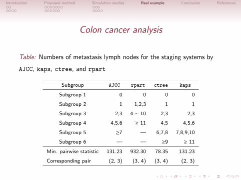
Colon cancer analysis
Table: Numbers of metastasis lymph nodes for the staging systems by
AJCC, kaps, ctree, and rpart
Subgroup AJCC rpart ctree kaps
Subgroup 1 0 0 0 0
Subgroup 2 1 1,2,3 1 1
Subgroup 3 2,3 4 ∼ 10 2,3 2,3
Subgroup 4 4,5,6 ≥ 11 4,5 4,5,6
Subgroup 5 ≥7 — 6,7,8 7,8,9,10
Subgroup 6 — — ≥9 ≥ 11
Min. pairwise statistic 131.23 932.30 78.35 131.23
Corresponding pair (2, 3) (3, 4) (3, 4) (2, 3)
Introduction Proposed method Simulation studies Real example Conclusion References
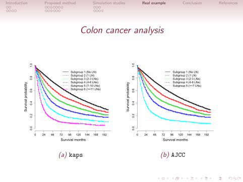
Colon cancer analysis
Survival months
Sur
viva
l pro
babi
lity
0.0
0.2
0.4
0.6
0.8
1.0
0 24 48 72 96 120 144 168 192
Subgroup 1 (No LN)Subgroup 2 (1 LN)Subgroup 3 (2-3 LNs)Subgroup 4 (4-6 LNs)Subgroup 5 (7-10 LNs)Subgroup 6 (>=11 LNs)
(a) kaps
Survival months
Sur
viva
l pro
babi
lity
0.0
0.2
0.4
0.6
0.8
1.0
0 24 48 72 96 120 144 168 192
Subgroup 1 (No LN)Subgroup 2 (1 LN)Subgroup 3 (2-3 LNs)Subgroup 4 (4-6 LNs)Subgroup 5 (>=7 LNs)
(b) AJCC
Introduction Proposed method Simulation studies Real example Conclusion References
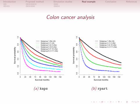
Colon cancer analysis
Survival months
Sur
viva
l pro
babi
lity
0.0
0.2
0.4
0.6
0.8
1.0
0 24 48 72 96 120 144 168 192
Subgroup 1 (No LN)Subgroup 2 (1 LN)Subgroup 3 (2-3 LNs)Subgroup 4 (4-6 LNs)Subgroup 5 (7-10 LNs)Subgroup 6 (>=11 LNs)
(a) kaps
Survival months
Sur
viva
l pro
babi
lity
0.0
0.2
0.4
0.6
0.8
1.0
0 24 48 72 96 120 144 168 192
Subgroup 1 (No LN)Subgroup 2 (1-3 LNs)Subgroup 3 (4-10 LNs)Subgroup 4 (>=11 LNs)
(b) rpart
Introduction Proposed method Simulation studies Real example Conclusion References
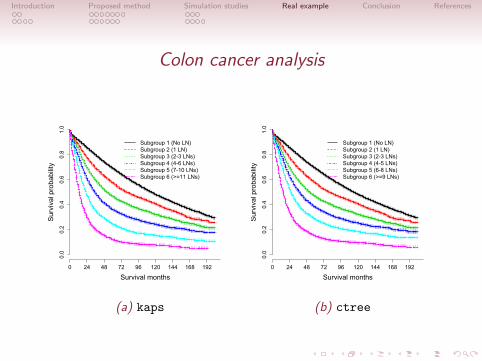
Colon cancer analysis
Survival months
Sur
viva
l pro
babi
lity
0.0
0.2
0.4
0.6
0.8
1.0
0 24 48 72 96 120 144 168 192
Subgroup 1 (No LN)Subgroup 2 (1 LN)Subgroup 3 (2-3 LNs)Subgroup 4 (4-6 LNs)Subgroup 5 (7-10 LNs)Subgroup 6 (>=11 LNs)
(a) kaps
Survival months
Sur
viva
l pro
babi
lity
0.0
0.2
0.4
0.6
0.8
1.0
0 24 48 72 96 120 144 168 192
Subgroup 1 (No LN)Subgroup 2 (1 LN)Subgroup 3 (2-3 LNs)Subgroup 4 (4-5 LNs)Subgroup 5 (6-8 LNs)Subgroup 6 (>=9 LNs)
(b) ctree

Introduction Proposed method Simulation studies Real example Conclusion References
Conclusion
We propose a multi-way partitioning algorithm for survival data,
• Divide the data into K heterogeneous subgroups based on the
information of a prognostic factor.
• Generate only fairly well-separated subgroups rather than a
mixture of extremely poorly and well-separated subgroups.
• Identify a multi-way partition which maximizes the minimum
of the pairwise test statistics among subgroups.
• Utilize a permutation test to consists of tow or more
cutpoints.
• Implement an add-on R package into kaps available at CRAN.

Introduction Proposed method Simulation studies Real example Conclusion References
Conclusion
• HJ Kang*, S-H Eo*, SC Kim, KM Park, YJ Lee, SK Lee, E Yu, H Cho,
and S-M Hong (2014). Increased Number of Metastatic Lymph Nodes in
Adenocarcinoma of the Ampulla of Vater as a Prognostic Factor: A
Proposal of New Nodal Classification, Surgery, 155:1, 74-84. (*:co-first
author)
• S-H Eo, S-M Hong, and H Cho (2014). K -adaptive partitioning for
survival data: the kaps add-on package for R, arXiv, 1306.4015v2.
• S-H Eo, S-M Hong, and H Cho. K -adaptive partitioning for survival
data, submitted to Statistics in Medicine.
• Park et al. Survival effect of tumor size and extrapancreatic extension in
surgically resected pancreas cancer patients: Proposal for improved T
classification, submitted to Surgery.

Introduction Proposed method Simulation studies Real example Conclusion References
Cecile Contal and John O’Quigley.
An application of changepoint methods in studying the effect of age on survival in breast cancer.
Computational Statistics and Data Analysis, 30:253–270, 1999.
S.B. Edge, D.R. Byrd, C.C. Compton, A.G. Fritz, F.L. Greene, and A. 3rd Trotti.
AJCC Cancer staging manual.
Springer, New York, 2010.
Susan Galloway Hilsenbeck and Gary M Clark.
Practical p-value adjustment for optimally selected cutpoints.
Statistics in Medicine, 15(1):103–112, 1996.
SM Hong, H Cho, C. Moskaluk, and E Yu.
Measurement of the invasion depth of extrahepatic bile duct carcinoma: An alternative method overcoming
the current t classification problems of the ajcc staging system.
American Journal of Surgical Pathology, 31:199–206, 2007.
Torsten Hothorn, Kurt Hornik, and Achim Zeileis.
Unbiased recursive partitioning: A conditional inference framework.
Journal of Computational and Graphical Statistics, 15(3), 2006.
Torsten Hothorn and Berthold Lausen.
On the exact distribution of maximally selected rank statistics.
Computational Statistics and Data Analysis, 43:121–137, 2003.
Hemant Ishwaran, Eugene H Blackstone, Carolyn Apperson-Hansen, and Thomas W Rice.
A novel approach to cancer staging: application to esophageal cancer.
Biostatistics, 10(4):603–620, 2009.

Introduction Proposed method Simulation studies Real example Conclusion References
Berthold Lausen, Willi Sauerbrei, and Martin Schumacher.
Classification and regression trees (cart) used for the exploration of prognostic factors measured on different
scales.
In P Dirschedl and R Ostermann, editors, Computational Statistics. Physica Verlag, Heidelberg, 1994.
Michael LeBlanc and John Crowley.
Relative risk trees for censored survival data.
Biometrics, pages 411–425, 1992.