journal title the trouble with the author(s) 2016 ... trouble with... · romer 3 figure 2. the...

The Trouble withMacroeconomics

Journal TitleXX(X):1–20c©The Author(s) 2016

Reprints and permission:sagepub.co.uk/journalsPermissions.navDOI: 10.1177/ToBeAssignedwww.sagepub.com/

Paul Romer1

AbstractIn the last three decades, the methods and conclusions of macroeconomics have deteriorated tothe point that much of the work in this area no longer qualifies as scientific research. The treatmentof identification in macroeconomic models is no more credible than in the first generation largeKeynesian models, and is worse because it is far more opaque. On simple questions of fact, such aswhether the Fed can influence the real fed funds rate, the answers verge on the absurd. The evolutionof macroeconomics mirrors developments in string theory from physics, which suggests that they areexamples of a general failure mode of for fields of science that rely on mathematical theory in whichfacts can end up being subordinated to the theoretical preferences of revered leaders. The largerconcern is that macroeconomic pseudoscience is undermining the norms of science throughouteconomics. If so, all of the policy domains that economics touches could lose the accumulation ofuseful knowledge that characteristic of true science, the greatest human invention.

KeywordsMacroeconomics, Science

Lee Smolin begins The Trouble with Physics (Smolin 2007) with an arresting observation. His careerspanned the only quarter-century in the history of physics when the field made no progress on its coreproblems. The trouble with macroeconomics is worse. I have observed more than three decades ofintellectual regress.

In the 1960s and early 1970s, many macroeconomists were cavalier about the identification problem.They did not appreciate how difficult it is to make reliable inferences about causality from observationson variables that are part of a simultaneous system. By the late 1970s, macroeconomists took this issuemore seriously. But as Canova and Sala (2009) signal with the title of a recent paper, we are now “Back toSquare One.” Macro models now use incredible assumptions to reach absurd conclusions. To appreciate

1New York University

Corresponding author:Paul Romer, Stern School of Business, New York University, New York, NY 10012.Email: [email protected]

Prepared using sagej.cls [Version: 2013/07/26 v1.00]

2 Journal Title XX(X)

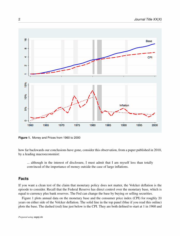
Figure 1. Money and Prices from 1960 to 2000

how far backwards our conclusions have gone, consider this observation, from a paper published in 2010,by a leading macroeconomist:

... although in the interest of disclosure, I must admit that I am myself less than totallyconvinced of the importance of money outside the case of large inflations.

Facts

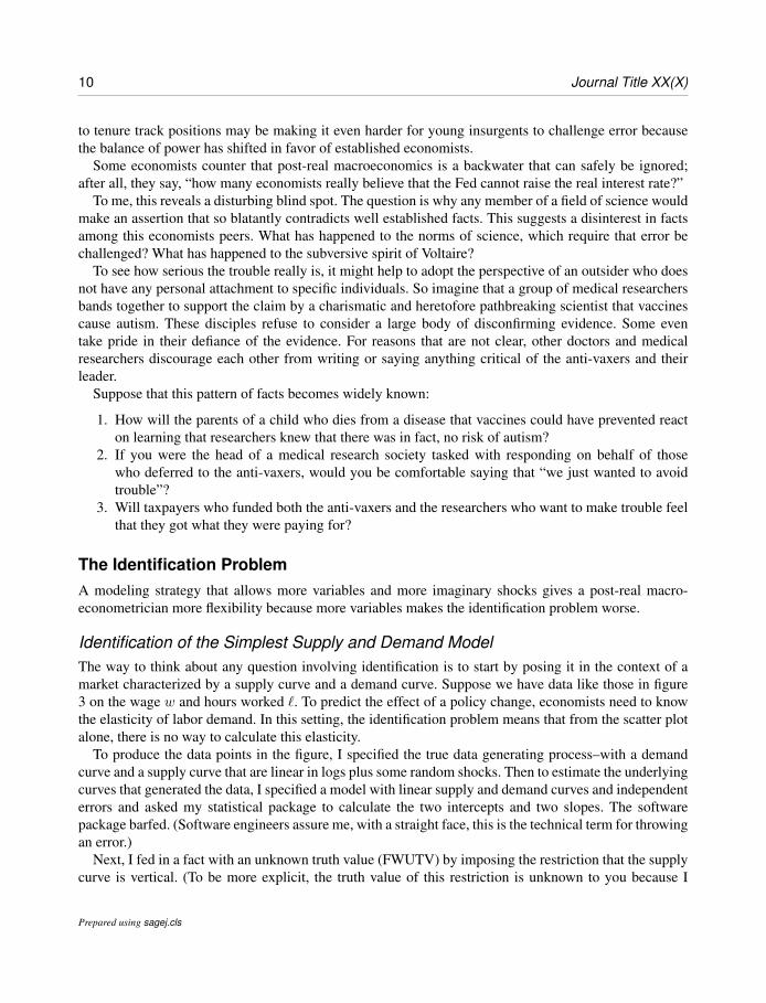
If you want a clean test of the claim that monetary policy does not matter, the Volcker deflation is theepisode to consider. Recall that the Federal Reserve has direct control over the monetary base, which isequal to currency plus bank reserves. The Fed can change the base by buying or selling securities.

Figure 1 plots annual data on the monetary base and the consumer price index (CPI) for roughly 20years on either side of the Volcker deflation. The solid line in the top panel (blue if you read this online)plots the base. The dashed (red) line just below is the CPI. They are both defined to start at 1 in 1960 and

Prepared using sagej.cls

Romer 3

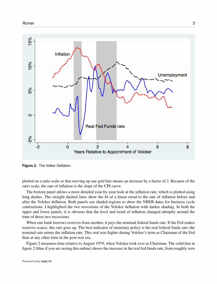
Figure 2. The Volker Deflation

plotted on a ratio scale so that moving up one grid line means an increase by a factor of 2. Because of theratio scale, the rate of inflation is the slope of the CPI curve.

The bottom panel allows a more detailed year-by-year look at the inflation rate, which is plotted usinglong dashes. The straight dashed lines show the fit of a linear trend to the rate of inflation before andafter the Volcker deflation. Both panels use shaded regions to show the NBER dates for business cyclecontractions. I highlighted the two recessions of the Volcker deflation with darker shading. In both theupper and lower panels, it is obvious that the level and trend of inflation changed abruptly around thetime of these two recessions.

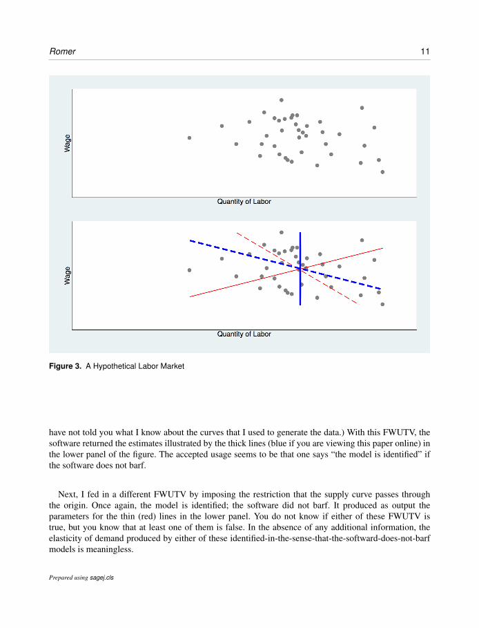
When one bank borrows reserves from another, it pays the nominal federal funds rate. If the Fed makesreserves scarce, this rate goes up. The best indicator of monetary policy is the real federal funds rate–thenominal rate minus the inflation rate. This real was higher during Volcker’s term as Chairman of the Fedthan at any other time in the post-war era.

Figure 2 measures time relative to August 1979, when Volcker took over as Chairman. The solid line infigure 2 (blue if you are seeing this online) shows the increase in the real fed funds rate, from roughly zero



to about 5%, that followed soon thereafter. The dashed (red) line shows a monthly measure of inflationcalculated as the change in the CPI over the previous 12 months. The (black) line with long dashesshows the unemployment rate, which in contrast to GDP, is available on a monthly basis. During the firstrecession, output fell by 2.2% as unemployment rose from 6.3% to 7.8%. During the second, output fellby 2.9% as unemployment increased from 7.2% to 10.8%.

In month 2, Volcker took the unusual step of holding a press conference to announce changes that theFed would adopt in its operating procedures. Romer and Romer (1989) summarize the internal discussionat the Fed that led up to this change. Fed officials expected that the change would cause a “prompt increasein the Fed Funds rate” and would “dampen inflationary forces in the economy.” The data from figure 2suggest a simple causal explanation for the events that is consistent with what they said:

1. The Fed aimed for a nominal Fed Funds rate that was roughly 500 basis points higher than theprevailing inflation rate, departing from this goal only during the first recession.

2. High real interest rates decreased output and increased unemployment.3. The rate of inflation fell, either because the combination of higher unemployment and a bigger

output gap caused it to fall or because the Fed’s actions changed expectations.

If the Fed can cause a 500 basis point change in interest rates, it is truly absurd to wonder if monetarypolicy is important. Faced with the data in figure 2, the only way to remain faithful to dogma that it is notimportant is to argue that despite what people at the Fed thought, it was actually an imaginary shock thatincreased real fed funds rate.

Post-Real ModelsMacroeconomists got comfortable with the idea that it is imaginary that shocks, rather than actions thatpeople take, after Kydland and Prescott (1982) launched the real business cycle (RBC) model. Stripped tois essentials, an RBC model relies on two identities. The first defines the usual growth-accounting residualas the difference between the growth of output Y and growth of an index X of inputs in production:

∆%A = ∆%Y − ∆%X

Abromovitz (1956) famously referred to this residual as “the measure of our ignorance.” In his honor andto remind ourselves of our ignorance, I will refer to the variable A a phlogiston.

The second identity, the quantity theory of money, defines velocity v as nominal output (real output Ytimes the price level P ) divided by the quantity of a monetary aggregate M :

v =Y P

M

The real business cycle model explains recessions as exogenous decreases in phlogiston. Given outputY , the only effect of a change in the monetary monetary aggregate M is a proportional change in theprice level P . In this model, the effects of monetary policy are so insignificant that, as Prescott taughtgraduate students at the University of Minnesota “postal economics is more central to understanding theeconomy than monetary economics” (Chong, La Porta, Lopez-de-Silanes, Shliefer, 2014).

Proponents of the RBC model cite as one of its main advantages its microeconomic foundation. Thisposed a problem because there is no microeconomic evidence for the negative phlogiston shocks that


Romer 5

the model invokes nor any sensible theoretical interpretation of what a negative phlogiston shock wouldmean.

In private correspondence, someone who overlapped with Prescott at the University of Minnesota sentme an account that reminded me of what it was like to encounter “negative technology shocks” beforewe became numb to them:

I was invited by Ed Prescott to serve as a second examiner at one of his student’s preliminaryoral. ... I had not seen or suspected the existence of anything like the sort of calibrationexercise the student was working on. There were lots of reasons I thought it didn’t havemuch, if any, scientific value, but as the presentation went on I made some effort to sortthem out, and when it came time for me to ask a question, I said (not even imagining that theconcept wasn’t specific to this particular piece of thesis research) “What are these technologyshocks?”

Ed tensed up physically like he had just taken a bullet. After a very awkward four or fiveseconds he growled “They’re that traffic out there.” (We were in a room with a view of someafternoon congestion on a bridge that collapsed a couple decades later.) Obviously, if hehad what he sincerely thought was a valid justification of the concept, I would have beenlistening to it ...

In response to the observation that the shocks are imaginary, a standard defense invokes MiltonFriedman’s (1953) methodological assertion from unnamed authority that “the more significant thetheory, the more unrealistic the assumptions.” More recently, “all models are false” seems to have becomethe universal hand-wave for dismissing any fact that does not conform to a favorite model.

The noncommittal relationship with the truth revealed by these methodological evasions and the “lessthan totally convinced ...” dismissal of fact goes so far beyond post-modern irony that it deserves its ownlabel. I suggest “post-real.”

DSGE Extensions to the RBC Core

More imaginary shocksOnce macroeconomists concluded that a macroeconomic aggregate could fluctuate in the absence ofany decision by any person, macroeconomists piled on extra imaginary driving forces. The resultingmenagerie, together with my suggested names now includes:

• A general type of phlogiston that increases the quantity of consumption goods produced by giveninputs

• An “investment-specific” type of phlogiston that increases the quantity of capital goods producedby given inputs

• A troll who makes random changes to the wages paid to all workers• A gremlin who makes random changes to the price of output• Aether, which increases the risk preference of investors• Caloric, which makes people want less leisure



With the possible exception of phlogiston, they assumed that there is no way to directly measure theseforces. In principle, phlogiston can in measured using the methods of growth accounting. In practice, thecalculated residual is very sensitive to mismeasurement of the utilization rate of inputs in production sothat even in this case, direct measurements are frequently ignored.

Sticky PricesTo allow for the possibility that monetary policy could matter, empirical DSGE models also put sticky-price lipstick on this RBC pig. The sticky-price extensions allow for the possibility that monetary policycan affect output, but the reported results from fitted or calibrated models never stray far from RBCdogma. If monetary policy matters at all, it matters very little.

As I will later, when the number of variables in a model increases, the identification problem gets muchworse. In practice, this means that the econometrician has more flexibility in determining the results thatemerge when she estimates the model.

The identification problem means that to get results, an econometrician has to feed something inother than observations on the variables in the system. I will refer to things that get fed in as facts withunknown truth value (FWUTV) to emphasize that although the estimation process treats the FWUTV’s asif they were facts known to be true, the process of estimating the model reveals nothing about the actualtruth value. The current practice in DSGE econometrics is pin down estimates not simply by feeding inFWUTV by “calibrating” the values of some parameters, but increasingly via tight Bayesian priors forother parameters. As Olivier Blanchard (2016) observes, “in many cases, the justification for the tightprior is weak at best, and what is estimated reflects more the prior of the researcher than the likelihoodfunction.”

This is more problematic that it seems because the prior specified for one parameter will typicallyhave a decisive influence on the output (a posterior distribution) for other parameters. This means thatthe econometrician can search for priors on seemingly unimportant parameters to find ones that yield theexpected result for the parameters of interest.

An ExampleThe Smets and Wouters (SW) model was hailed as a breakthrough success for DSGE econometrics.When they applied this model to data from the United States for years that include the Volcker deflation,Smets and Wouters (2007) conclude:

...monetary policy shocks contribute only a small fraction of the forecast variance of outputat all horizons.

...monetary policy shocks account for only a small fraction of the inflation volatility.

...[In explaining the correlation between output and inflation:] Monetary policy shocks donot play a role for two reasons. First, they account for only a small fraction of inflation andoutput developments.

What matters in the is not money but the imaginary forces. Here is what the authors say about them,modified only by substituting my suggested alternative names (in bold) for these forces:


Romer 7

While “demand” shocks such as the aether, exogenous spending, and investment-specificphlogiston shocks explain a significant fraction of the short-run forecast variance inoutput, both the troll’s wage mark-up (or caloric) and, to a lesser extent, output-specificphlogiston shocks explain most of its variation in the medium to long run. ... Third, inflationdevelopments are mostly driven by the gremlin’s price mark-up shocks in the short run andthe troll’s wage mark-up shocks in the long run.

A footnote in a subsequent paper (Linde, Smets, Wouters 2016) underlines the flexibility that imaginarydriving forces bring to post-real macroeconomics (once again with my suggestions for names):

The prominent role of the gremlin’s price and troll’s wage markup for explaining inflationand behavior of real wages in the SW-model have been criticized by Chari, Kehoe andMcGrattan (2009) as implausibly large. Gal, Smets and Wouters (2011), however, shows thatthe size of the markup shocks can be reduced substantially by allowing for caloric shocks tohousehold preferences.

Questions About Economists, and PhysicistsI find that it helps to separate the standard questions of macroeconomics, such as whether the Fed caninfluence increase the real fed funds rate, from meta-questions about how what economists do whenthey try to answer the standard questions. One example of a meta-question is why macroeconomistsstarted invoking imaginary driving forces to explain fluctuations. A more revealing one is why thereare such striking parallels between the characteristics of string-theorists in particle physics and post-realmacroeconomists.

To illustrate the similarity, I will reproduce Smolin’s list (from Chapter 16) of seven distinctivecharacteristics of string theorists:

1. Tremendous self-confidence2. An unusually monolithic community3. A sense of identification with the group akin to identification with a religious faith or political

platform4. A strong sense of the boundary between the group and other experts5. A disregard for and disinterest in ideas, opinions, and work of experts who are not part of the group6. A tendency to interpret evidence optimistically, to believe exaggerated or incomplete statements of

results, and to disregard the possibility that the theory might be wrong7. A lack of appreciation for the extent to which a research program ought to involve risk

My conjecture is that string theory and post-real macroeconomics illustrate a general failure mode ofa scientific field that relies on mathematical theory. The conditions for failure are present when a fewtalented researchers come to be respected for genuine contributions on the cutting edge of mathematicalmodeling. Admiration evolves into deference to these leaders. Deference leads to effort along the specificlines that the leaders recommend. Because guidance from authority can coordinate the efforts of otherresearchers, conformity to the facts is no longer needed as a coordinating device. As a result, if factsdisconfirm the officially sanctioned theoretical vision, they are subordinated. Eventually, evidence stops



being relevant. Progress in the field is judged by the purity of its mathematical theories, as determined bythe authorities.

One of the surprises in Smolin’s account is his rejection of the excuse offered by the string theorists,that they do not pay attention to data because there is no practical way to collect data on energies at thescale that that string theory considers. He makes a convincing case that are plenty of unexplained facts thatthe theorists could have addressed if they had wanted to (Chapter 13). In physics as in macroeconomics,the disregard for evidence and facts was a choice.

Smolin’s argument lines up almost perfectly with a taxonomy for collective human effort proposed byMario Bunge (1984). It starts by distinguishing “research” fields from “belief” fields. In research fieldssuch as math, science, and technology, the pursuit of truth is the coordinating device. In belief fields suchas religion, and political action, authorities coordinate the efforts of the groups members.

There is nothing inherently bad about coordination by authorities. Sometimes there is no alternative.The abolitionist movement was a belief field that relied on authorities to make such decisions as whetherits members should treat the incarceration of criminals as slavery. Some authority had to make thisdecision because there is no logical argument, nor any fact, that group members could use independentlyto resolve it question.

In Bunge’s taxonomy, pseudoscience is a special type of belief field that claims to be science. Itis dangerous because research fields are sustained by norms that are different from those of a belieffield. Because norms spread through social interaction, pseudoscientists who mingle with scientists canundermine the norms that are essential for science to survive. Revered individuals are unusually importantin shaping the norms of a field, particularly in the role of teachers who bring new members into the field.For this reason, an efficient defense of science will hold the most highly regarded individuals to thehighest standard of scientific conduct.

A Meta-Model of MeIn the distribution of commentary about the state of macroeconomics, my pessimistic assessment ofregression into pseudoscience lies in the extreme lower tail. Most of the commentary acknowledges roomfor improvement, but celebrates steady progress, at least as measured by a post-real metric that valuesmore sophisticated tools. A natural question to ask is why there are so few other voices saying what I say.

A model of me that explains my different choices should trace them back to different preferences,different prices, or different information sets. Others see the same papers and have participated in thesame discussions, so we can dismiss asymmetric information.

To first order, it seems reasonable to assume that all economists have the same preferences. We all takesatisfaction from the professionalism of doing our job well. Doing the job well means disagreeing openlywhen someone makes an assertion that seems wrong.

When the person who says something that seems wrong is a revered leader of a group with thecharacteristics Smolin lists, there is a price to be paid for disagreeing with openly. This price is lowerfor me because I am no longer an academic. I am a practitioner, by which I mean that I want to putuseful knowledge to work. I care little about whether I ever publish again in leading economics journalsor receive any professional honor because neither will be of much help in putting useful insights to work.As a result, the standard threats that members of a group with Smolin’s characteristics can make do notapply.


Romer 9

The Norms of Science

Some of the economists who agree about the state of macro in private conversations with me will notsay so in public. This is consistent with the explanation based on different prices. Yet some of them alsodiscourage me from disagreeing openly.

My sense is that some of these economists have assimilated a norm that the post-real macroeconomistsactively promote–that is an extremely serious violation of some honor code for anyone to criticize openlya revered authority figure. The emotions this type of affront invokes are intense. After I criticized a paperby Lucas, I encountered by chance one of his friends. He was so angry that he could not find words tosay. Finally told me “you are killing Bob.” The other possibility is that these economists who agree butrecommend self-censorship simply want to avoid being confronted by the emotions that any criticismwill unleash.

A norm that places an authority above criticism helps people cooperate as members of a belief field thatpursues political, moral, or religious objectives. It is likely to be invoke more intense emotions when thegroup feels threatened and members need to cooperate in its defense. As Jonathan Haidt (2012) observes,this norm is supported by two innate moral senses, one that encourages us to defer to authority, anotherwhich compels self-sacrifice to defend the purity of the sacred.

The research fields spawned by the enlightenment survive by “turning the dial to zero” on these innatemoral senses. Members cultivate the conviction that nothing is sacred and that authority should always bechallenged. In this sense, Voltaire is more important to the intellectual foundation of the research fieldsof the enlightenment than Descartes or Newton.

By rejecting any reliance on central authority, the members of a research field can coordinate theirindependent efforts only by maintaining an unwavering commitment to truth, established imperfectly,via the rough consensus that emerges from many independent assessments of publicly disclosed factsand logic; assessments that are made by people who honor clearly stated disagreement, who accept theirown fallibility, and relish the chance to subvert any claim of to authority, not to mention any claim ofinfallibility.

A research field breaks down when members start taking cues from leaders who seem to know better.These authorities may activate the sense of duty that members have to defend the group and protect thepurity of the sacred. This will be easier if this group is indeed facing an intellectual threat.

Even with it works well, science is not perfect. Nothing that involves people ever is. At best, scienceestablishes the truth of an assertion in the same loose sense that the stock market establishes the valueof a firm. It can go astray, perhaps for long stretches of time, but is eventually yanked back to reality byinsurgents who periodically burst a bubble that allows a divergence from the facts.

Despite its evident flaws, science has been remarkably good at producing useful knowledge. It is alsoa uniquely benign way to coordinate large numbers of people, the only one that has ever established aconsensus that extends to millions or billions without using coercion.

The Threat Facing Economics

Whatever the mix of norms and intimidation that sustains them, I have watched conformism, deferenceto authority, and a commitment to purity that is more sacred than facts gain ground in economics for thelast 30 years. In the opinion of others I have spoken to, an increase in the supply of new Ph.D.s relative



to tenure track positions may be making it even harder for young insurgents to challenge error becausethe balance of power has shifted in favor of established economists.

Some economists counter that post-real macroeconomics is a backwater that can safely be ignored;after all, they say, “how many economists really believe that the Fed cannot raise the real interest rate?”

To me, this reveals a disturbing blind spot. The question is why any member of a field of science wouldmake an assertion that so blatantly contradicts well established facts. This suggests a disinterest in factsamong this economists peers. What has happened to the norms of science, which require that error bechallenged? What has happened to the subversive spirit of Voltaire?

To see how serious the trouble really is, it might help to adopt the perspective of an outsider who doesnot have any personal attachment to specific individuals. So imagine that a group of medical researchersbands together to support the claim by a charismatic and heretofore pathbreaking scientist that vaccinescause autism. These disciples refuse to consider a large body of disconfirming evidence. Some eventake pride in their defiance of the evidence. For reasons that are not clear, other doctors and medicalresearchers discourage each other from writing or saying anything critical of the anti-vaxers and theirleader.

Suppose that this pattern of facts becomes widely known:

1. How will the parents of a child who dies from a disease that vaccines could have prevented reacton learning that researchers knew that there was in fact, no risk of autism?

2. If you were the head of a medical research society tasked with responding on behalf of thosewho deferred to the anti-vaxers, would you be comfortable saying that “we just wanted to avoidtrouble”?

3. Will taxpayers who funded both the anti-vaxers and the researchers who want to make trouble feelthat they got what they were paying for?

The Identification ProblemA modeling strategy that allows more variables and more imaginary shocks gives a post-real macro-econometrician more flexibility because more variables makes the identification problem worse.

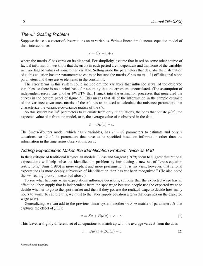
Identification of the Simplest Supply and Demand ModelThe way to think about any question involving identification is to start by posing it in the context of amarket characterized by a supply curve and a demand curve. Suppose we have data like those in figure3 on the wage w and hours worked `. To predict the effect of a policy change, economists need to knowthe elasticity of labor demand. In this setting, the identification problem means that from the scatter plotalone, there is no way to calculate this elasticity.

To produce the data points in the figure, I specified the true data generating process–with a demandcurve and a supply curve that are linear in logs plus some random shocks. Then to estimate the underlyingcurves that generated the data, I specified a model with linear supply and demand curves and independenterrors and asked my statistical package to calculate the two intercepts and two slopes. The softwarepackage barfed. (Software engineers assure me, with a straight face, this is the technical term for throwingan error.)

Next, I fed in a fact with an unknown truth value (FWUTV) by imposing the restriction that the supplycurve is vertical. (To be more explicit, the truth value of this restriction is unknown to you because I


Romer 11

Figure 3. A Hypothetical Labor Market

have not told you what I know about the curves that I used to generate the data.) With this FWUTV, thesoftware returned the estimates illustrated by the thick lines (blue if you are viewing this paper online) inthe lower panel of the figure. The accepted usage seems to be that one says “the model is identified” ifthe software does not barf.

Next, I fed in a different FWUTV by imposing the restriction that the supply curve passes throughthe origin. Once again, the model is identified; the software did not barf. It produced as output theparameters for the thin (red) lines in the lower panel. You do not know if either of these FWUTV istrue, but you know that at least one of them is false. In the absence of any additional information, theelasticity of demand produced by either of these identified-in-the-sense-that-the-softward-does-not-barfmodels is meaningless.



The m2 Scaling ProblemSuppose that x is a vector of observations on m variables. Write a linear simultaneous equation model oftheir interaction as

x = Sx+ c+ ε.

where the matrix S has zeros on its diagonal. For simplicity, assume that based on some other source offactual information, we know that the errors in each period are independent and that none of the variablesin x are lagged values of some other variable. Setting aside the parameters that describe the distributionof ε, this equation has m2 parameters to estimate because the matrix S has m(m− 1) off-diagonal slopeparameters and there are m elements in the constant c.

The error terms in this system could include omitted variables that influence serval of the observedvariables, so there is no a priori basis for assuming that the errors are uncorrelated. (The assumption ofindependent errors was another FWUTV that I snuck into the estimation processes that generated thecurves in the bottom panel of figure 3.) This means that all of the information in the sample estimateof the variance-covariance matrix of the x’s has to be used to calculate the nuisance parameters thatcharacterize the variance-covariance matrix of the ε’s.

So this system has m2 parameters to calculate from only m equations, the ones that equate µ(x), theexpected value of x from the model, to x̄, the average value of x observed in the data.

x̄ = Sµ(x) + c.

The Smets-Wouters model, which has 7 variables, has 72 = 49 parameters to estimate and only 7equations, so 42 of the parameters that have to be specified based on information other than theinformation in the time series observations on x.

Adding Expectations Makes the Identification Problem Twice as BadIn their critique of traditional Keynesian models, Lucas and Sargent (1979) seem to suggest that rationalexpectations will help solve the identification problem by introducing a new set of “cross-equationrestrictions.” Sims (1980) is more explicit and more pessimistic. “It is my view, however, that rationalexpectations is more deeply subversive of identification than has yet been recognized.” (He also notedthe m2 scaling problem described above.)

To see what happens when expectations influence decisions, suppose that the expected wage has aneffect on labor supply that is independent from the spot wage because people use the expected wage todecide whether to go to the spot market and then if they go, use the realized wage to decide how manyhours to work. To capture this, we must to the labor supply equation a term that depends on the expectedwage µ(w).

Generalizing, we can add to the previous linear system another m×m matrix of parameters B thatcaptures the effect of µ(x):

x = Sx+Bµ(x) + c+ ε. (1)

This leaves a slightly different set of m equations to match up with the average value x̄ from the data:

x̄ = Sµ(x) +Bµ(x) + c (2)


Romer 13

From these m equations, the challenge now is to calculate twice as many parameters, 2m2. In asystem with seven variables, this means 2 ∗ 72 − 7 = 91 parameters that have to be specified based oninformation other than what is in time series for x.

Moreover, in the absence of some change to a parameter or to the distribution of the errors, the expectedvalues x will be constant, so even with with arbitrarily many observations on x and all the knowledgeone could possibly hope for about the slope coefficients in S, it will still be impossible to disentangle theconstant term c from the expression Bµ(x). (Sims attributes this point to Solow,1974.)

So allowing for the possibility that expectations influence what happens makes the identificationproblem is twice as bad.

Regress in the Discussion of the Identification ProblemPost-real macroeconomists have not delivered the careful attention to the identification problem thatLucas and Sargent (1979) promised. They still rely on FWUTV. All they have done is learn how to makethis reliance more opaque.

Natural ExperimentsIn the analysis of a simultaneous system with many interacting variables, there is a solution to theidentification problem, the one that medical researchers have used with great success to find treatmentsfor disease: Do experiments. For macroeconomists, this means looking for natural experiments. This isthe path that Milton Friedman and Anna Schwartz started down when the made their case that monetarypolicy influenced output during the Great Depression.

Faced with the challenge of estimating the elasticity of labor demand in our simple supply and demandmarket, the method of Friedman and Schwartz would be to look for two periods that are adjacent in time,with conditions that were very similar, except for some change that shifts the labor supply curve in oneperiod relative to the other. To find this pair, they would look carefully at historical evidence that is notcontained in the scatter plot of the wage and labor supply.

If the historical circumstance offer up just one such pair, they would ignore all the other data points andbase an estimate on just these two. If Lucas and Sargent (1979) are correct that the identification problemis the most important problem in empirical macroeconomics, it makes makes sense to throw away data.It is better to have a meaningful estimate with a larger standard error (even one based on a single pair sothat we cannot even estimate the standard error from the data sample) than a meaningless estimate witha small standard error.

The Friedman and Schwartz approach allows cumulative scientific analysis of data because otherscan work to establish the truth value of the fact that this approach feeds in. For example, Romer andRomer (1989) challenge some of the facts that Friedman and Schwartz used from the history of theGreat Depression, and suggest that we have more reliable identifying information about episodes fromthe post-war period, especially the Volcker deflation.

When I was in graduate school, I was impressed by the Friedman Schwartz account of the increase inreserve requirements that caused the sharp recession of 1938-9. Romer and Romer (1989) suggest thatthis is not as clean a natural experiment as Friedman and Schwartz suggest. Now my estimate of the effectthat monetary policy can have on output in the United States relies much more heavily on the cleanestexperiment–the Volcker deflation.



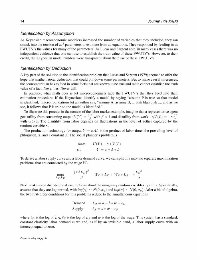
Identification by AssumptionAs Keynesian macroeconomic modelers increased the number of variables that they included, they ransmack into the tension of m2 parameters to estimate from m equations. They responded by feeding in asFWUTV’s the values for many of the parameters. As Lucas and Sargent note, in many cases there was noindependent evidence that one can use to establish the truth value of these FWUTV’s. However, to theircredit, the Keynesian model builders were transparent about their use of these FWUTV’s.

Identification by DeductionA key part of the solution to the identification problem that Lucas and Sargent (1979) seemed to offer thehope that mathematical deduction that could pin down some parameters. But to make causal inferences,the econometrician has to feed in some facts that are known to be true and math cannot establish the truthvalue of a fact. Never has. Never will.

In practice, what math does is let macroeconomists hide the FWUTV’s that they feed into theirestimation procedure. If the Keynesians identify a model by saying “assume P is true so that modelis identified,” micro-foundations let an author say, “assume A, assume B, ... blah blah blah .... and as wesee, it follows that P is true so the model is identified.”

To illustrate this process in the context of the labor market example, imagine that a representative agentgets utility from consuming output U(Y ) = Y β

β with β < 1 and disutility from work −γV (L) = −γ Lα

αwith α > 1. The disutility from labor depends on fluctuations in the level of aether captured by therandom variable γ.

The production technology for output Y = πAL is the product of labor times the prevailing level ofphlogiston, π, and a constant A. The social planner’s problem is

max U(Y ) − γ ∗ V (L)

s.t. Y = π ∗A ∗ L

To derive a labor supply curve and a labor demand curve, we can split this into two separate maximizationproblems that are connected by the wage W .

maxLS ,LD

(πALD)β

β−WD ∗ LD +WS ∗ LS − γ

LSα

α

Next, make some distributional assumptions about the imaginary random variables, γ and π. Specifically,assume that they are log normal, with log(γ) ∼ N(0, σγ) and log(π) ∼ N(0, σπ). After a bit of algebra,the two first-order conditions for this problems reduce to the simultaneous equations

Demand `D = a− b ∗ w + εD

Supply `S = d ∗ w + εS

where `D is the log of LD, `S is the log of LS and w is the log of the wage. This system has a standard,constant elasticity labor demand curve and, as if by an invisible hand, a labor supply curve with anintercept equal to zero.


Romer 15

With enough math, an author can be confident that most readers will never figure out where a FWUTVis buried. A discussant or referee cannot say that an identification assumption is not credible if theycannot figure out what it is and are too embarrassed to ask.

In this example, the FWUTV is that the mean of log(γ) is zero. Distributional assumptions about errorterms are a good place to bury things because hardly anyone pays attention to them. Moreover, if a criticdoes see that this is the identifying assumption, how will she win an argument about the true expectedvalue of the variable that tracks fluctuations in the level of aether? If the author can make up an imaginaryvariable, “because I say so” seems like a pretty convincing answer to any question about its properties.

Identification by ObfuscationI never understood how identification was achieved in the current crop of empirical DSGE models. Inpart, they rely on the type of identification by deduction illustrated in the previous section. They also relyon calibration, which is the renamed version of identification by assumption. But I never knew if therewere other places where FWUTV’s were buried. The papers that report the results of these empiricalexercises do not discuss the identification problem. For example, in Smets and Wooters (2007), neitherthe word “identify” nor “identification” appear.

To replicate the results from that model, so I read the User’s Guide for the software package, Dynare,that the authors used. In listing the advantages of the Bayesian approach, the User’s Guide says:

Third, the inclusion of priors also helps identifying parameters. (p. 78)

Reading this was a revelation. Being a Bayesian means that your software will never barf.In retrospect, this point should have been easy to see. To generate the thin curves in figure 3, I used as a

FWUTV the restriction that the intercept of the supply curve is zero. This is like putting a very tight prioron this parameter, centered at zero. If I loosen up the prior a little bit and calculate a Bayesian estimateinstead of a maximum likelihood estimate, I should get a value for the elasticity of demand that is almostthe same.

If I do this, the Bayesian procedure will show that the posterior of the intercept for the supply curve isclose to the prior distribution that I feed in. So in the jargon, I could say that “the data are not informativeabout the value of the intercept of the supply curve.” But then I could say that “the value of the slopeof the demand curve, has a tight posterior that is different from its prior.” By omission, the reader couldinfer that it is the data, as captured in the likelihood function, that are informative about the elasticity ofthe demand curve when in fact it is the prior on the intercept of the supply curve that pins it down andyields a tight posterior. By changing the priors I feed in for the supply curve, I can change the posteriorsI get out for the elasticity of demand until I get one I like.

Understanding how priors can carry FWUTV’s was a revelation for me, but it was apparently an opensecret for people who work in this field. In the paper with the title that I note in the introduction, Canovaand Sala (2009) write that “uncritical use of Bayesian methods, including employing prior distributionswhich do not truly reflect spread uncertainty, may hide identification pathologies.” Onatski and Williams(2010) show that if you feed different priors into an earlier version of the Smets and Wooters model(2003), you get back different structural estimates. Iskrev (2010) and Komunjer and Ng (2011) notethat without any information from the priors, Smets and Wooter model is not identified. Baumeister andHamilton (2015) note that in a bivariate vector autoregression for a supply and demand market that isestimated using Bayesian methods, it is quite possible that “even if one has available an infinite sample



of data, any inference about the demand elasticity is coming exclusively from the prior distribution.”Reicher (2015) echos the point that Sims made in his discussion of the results of Hatanaka (1975): “Thestructural parameters governing DSGE models are not identified when the driving process behind themodel follows an unrestricted VAR.”

Loyalty Can Corrode The Norms of ScienceThe description of the failure mode of science presented above might be construed as a warning that thethreat to science comes from self-interest. This would be a serious misreading of the model of sciencethat guides this analysis. People are always motivated by self-interest. Science would never have survivedif it required its participants to be selfless saints.

Like the market, science is a social system that uses competition to direct the self-interest of theindividual to the advantage of the group. The problem is that competition in science, like competitionin the market, is vulnerable to collusion.

Bob Lucas, Ed Prescott, and Tom Sargent lead the development of post-real macroeconomics. Priorto 1980, they made important scientific contributions to macroeconomic theory. They shared experience“in the foxhole” when these contributions provoked return fire that could be sarcastic, dismissive, andwrong-headed. As a result, they developed a bond of loyalty that would be admirable and productive inmany social contexts.

E. M. Forster wrote “If I had to choose between betraying my country and betraying my friend I hopeI should have the guts to betray my country.” If you substitute “science” in place of “country,” it is nothard to imagine that for many people, choice would still be to support the friend. Unfortunately, this typeof loyalty can undermine the competition that science counts on.

Two examples will be sufficient to illustrate the bias that loyalty can introduce.

Example 1: Lucas Supports PrescottIn his 2003 Presidential Address to the American Economics Association, Lucas gave a strongendorsement to Prescott’s claim that monetary economics was a triviality.

This position is hard to reconcile with Lucas’s 1995 Nobel lecture, which gives a nuanced discussionof the reasons for thinking that monetary policy does matter and the theoretical challenge that this posesfor macroeconomic theory. It is also inconsistent with his comments (Lucas, 1994) on a paper by Ball andMankiw (1994), in which he wrote that that Cochrane (1994) gives “an accurate view of how little cansaid to be firmly established about the importance and nature of the real effects of monetary instability,at least for the U.S. in the postwar period.”

Cochrane notes that if money has the type of systematic effects that his VAR’s suggest, it was moreimportant to study such elements of monetary policy as the role of lender of last resort and such monetaryinstitutions as deposit insurance than to make “an assessment of how much output can be furtherstabilized by making monetary policy more predictable.” According to Cochrane, if this assessmentsuggests tiny benefits, “it may not be the answers that are wrong; we may simply be asking the wrongquestion.”

Nevertheless, Lucas (2003) considers the effect of making monetary policy more predictable andconcludes that the potential welfare gain is indeed small, “on the order of hundredths of a percent ofconsumption.”


Romer 17

In an introduction to his collected papers published in 2013, Lucas conceded Cochran’s point, thatit would have been important to study the role of the Fed as lender of last resort. He writes that hisconclusion in the 2003 address was that in the postwar era in the U.S., monetary factors had not been“a major source of real instability over this period, not that they could not be important or that theynever had been. I shared Friedman and Schwartz’s views on the contraction phase, 1929-1933, of theGreat Depression, and this is also the way I now see the post-Lehman 2008-2009 phase of the currentrecession.” (Italics in the original.)

Lucas (2003) also endorses Prescott’s (1986) calculation that 84% of output variability is due tophlogiston/technology shocks, even though Cochrane also reported results showing that the t-statisticon this estimate would be roughly 1.2 so the usual two standard-error confidence interval includes theentire range of possible values, [0%, 100%]. In fact, Cochrane’s table 12 shows that economists whotried to calculate this fraction using other methods came up with estimates that fill the entire range fromPrescott estimate of about 80% down to 0.003%, 0.002% and 0%.

The only possible explanation I can see for the strong claims that Lucas makes in his 2003 lecturerelative to what he wrote before and after is that in the lecture, he was doing his best to support his friend,Prescott.

Example 2: Sargent Supports LucasA second example of arguments that go above and beyond the call of science is the defense that TomSargent offered for a paper by Lucas (1980) on the quantity theory of money. In the 1980 paper, Lucasestimated a demand for nominal money and found that it was proportional to the price level, as thequantity theory predicts. He found a way to filter the data to get the quantity theory result in the specificsample of U.S. data that he considered (1953-1977) and implicitly seems to have concluded that whateveridentifying assumptions were built into his filter must have been correct because the results that came outsupported the quantity theory. (Whiteman 1984 showed how to work out explicitly what those identifyingassumptions were for the filter Lucas used.)

Sargent and Surico (2011) revisit Lucas’s approach and show when it is applied to data after the Volckerdeflation, his method yields a very different result. They show that the change could arise from a changein the money supply process.

In making this point, they go out of their way to portray Lucas’s 1980 paper in the most favorableterms. Lucas wrote that his results may be of interest as “a measure of the extent to which the inflationand interest rate experience of the postwar period can be understood in terms of purely classical, monetaryforces.” Sargent and Surico give this sentence the implausible interpretation that “Lucas’s purpose ... wasprecisely to show that his result depends for its survival on the maintenance of the money supply processin place during the 1953-1977 period.”

They also misrepresent the meaning of the comment Lucas makes that there are conditions in whichthe quantity theory might break down. From the context it is clear that what Lucas means is that thequantity theory will not hold for the high-frequency variation that his filtering method removes. It is not,as Sargent and Surico suggest, a warning that the filtering method will yield different results if the Fedwere to adopt a different money supply rule.

The simplest way to describe their result is to say that using Lucas’s estimator, the exponent on theprice level in the demand for money is identified (in the sense that it yields a consistent estimator for the



true parameter) only under restrictive assumptions about money supply, but Sargent and Surico do notdescribe their results this way.

In fact, they never mention identification, even though they estimate their own structural DSGE modelso they can carry out their policy experiment and ask “What happens if the money supply rule changes?”They never discuss the identifying assumptions that feed in the facts that their estimation procedure needsto generate structural parameters as outputs. They say that they relied on a Bayesian estimation procedureand as usual, several of the parameters have priors and posteriors that are very similar.

Had a traditional Keynesian written the 1980 paper and offered the estimated demand curve for moneyas an equation that could be added into a 1970 vintage multi-equation Keynesian model, I expect thatSargent would have responded with much greater clarity. In particular, I doubt that in this alternativescenario, he would have offered the response in footnote 2 to the the question that someone (perhaps areferee) posed about identification:

Furthermore, DSGE models like the one we are using were intentionally designed asdevices to use the cross-equation restrictions emerging from rational expectations modelsin the manner advocated by Lucas (1972) and Sargent (1971), to interpret how regressionsinvolving inflation would depend on monetary and fiscal policy rules. We think that we areusing our structural model in one of the ways its designers intended.

Lucas and Sargent (1979, p. 52) includes this statement: “The problem of identifying a structural modelfrom a collection of economic time series is one that must be solved by anyone who claims the abilityto give quantitative economic advice.” It offers no exemption for authorities that lets them respond bysaying “we know what we are doing and do not have to answer your question about identification.”

Conclusion: Back to Square OneI agree with the harsh judgment that Lucas and Sargent (1979) made about the macro models of their day–that they relied on identifying assumptions that were not credible. The situation now is worse. Modelsmake assumptions that are no more credible and far more opaque.

I also agree with the harsh judgment that Lucas and Sargent made about the predictions of thoseKeynesian models, the prediction that an increase in the inflation rate would cause a reduction in theunemployment rate.

Lucas (2003) introduces his Presidential lecture to the American Economics Association by saying:

My thesis in this lecture is that macroeconomics in this original sense has succeeded: Itscentral problem of depression prevention has been solved, for all practical purposes, and hasin fact been solved for many decades. There remain important gains in welfare from betterfiscal policies, but I argue that these are gains from providing people with better incentivesto work and to save, not from better fine-tuning of spending flows. Taking U.S. performanceover the past 50 years as a benchmark, the potential for welfare gains from better long-run,supply-side policies exceeds by far the potential from further improvements in short-rundemand management.

Using the worldwide loss of output as a metric, for Lucas, the financial crisis of 2008-9 is a failedprediction that is much more serious than the failure of the Keynesian models. So what Lucas and


Romer 19

Sargent wrote of Keynesian macro models applies with full force today to post-real macro models andthe program that generated them:

That these predictions were wildly incorrect, and that the doctrine on which they were basedis fundamentally flawed, are now simple matters of fact ...

... the task that faces contemporary students of the business cycle is that of sorting throughthe wreckage ...

Someday, medicine might reach a point where any of us would be willing to let a dynamic stochasticsimultaneous equations equilibrium model of the human body determine which course of treatment wefollow for a family member faced with a life-threatening disease. It is not at this point now. As far asI can tell, no one in medicine sees work on such a model as a practical path toward better treatment ofdisease.

Perhaps this time, macroeconomists should admit that the wreckage runs so deep that they shouldabandon the quest for the sacred simultaneous equation model. It might be wiser to adopt the messymethods that medical researchers have used to make discoveries that were implemented and actuallyimproved health.

ReferencesAbramovitz M (1965). “Resource and Output Trends in the United States Since 1870.” Resource and

Output Trends in the United States Since 1870, NBER, p. 1-23.Ball L and Mankiw G (1994). “A Sticky-Price Manifesto.” Carnegie Rochester Conference Series on

Public Policy, Vol. 41, p. 127-151.Baumeister C and Hamilton J (2015). “Sign Restrictions, Structural Vector Autoregressions, and Useful

Prior Information.” Econometrica, Vol. 83, No. 5, p. 1963-1999.Blanchard O (2016). “Do DSGE Models Have a Future?” Peterson Institute of International Economics,

PB 16-11.Bunge M (1984). “What is Pseudoscience?” The Skeptical Inquirer, Vol. 9, p. 36-46.Canova F and Sala L (2009). “Back to Square One.” Journal of Monetary Economics, Vol. 56, p. 431-449.Cochrane J (1994). “Shocks.” Carnegie Rochester Conference Series on Public Policy, Vol. 41, p. 295-

364.Chong A, La Porta R, Lopez-de-Silanes F, Shliefer A (2014). “Letter grading government efficiency.”

Journal of the European Economic Association, Vol. 12, No. 2, p. 277-299.Hatanaka M (1975). “On the Global Identification Problem of the Dynamic Simultaneous Equation

Model,” International Economic Review, Vol. 16, p. 138-148.Iskrev N (2010). “Local Identification in DSGE Models.” Journal of Monetary Econommics, Vol. 57, p.

189-202.Kydland F and Prescott E (1982). “Time to build and aggregate fluctuations.” Econometrica, Vol. 50, No.

6, p. 1345-1370.Komunjer I and Ng S (2011). “Dynamic Identification of Stochastic General Equilibrium Models.”

Econometrica, Vol. 76, No. 6, p. 1995-2032.Linde J, Smets F and Wouters R (2016). “Challenges for Central Banks’ Models,” Sveriges Riksbank

Research Paper Series, 147.



Lucas R (1972). “Econometric Testing of the Natural Rate Hypothesis.” In Econometrics of PriceDetermination, e.d. Otto Eckstein, Board of Governors of the Federal Reserve System, p. 50-59.

Lucas R (1980). “Two Illustrations of the Quantity Theory of Money,” American Economic Review, Vol.70, No. 5, p. 1005-10014.

Lucas R (1994). “Comments on Ball and Mankiw.” Carnegie Rochester Conference Series on PublicPolicy, Vol. 41, p. 153-155.

Lucas R (2003). “Macroeconomic Priorities.” American Economic Review, Vol. 93, No. 1, p. 1-14.Lucas R and Sargent T (1989). “After Keynsian Macroeconomics.” After The Phillips Curve: Persistence

of High Inflation and High Unemployment, Federal Reserve Board of Boston.Onatski A and Williams N (2010). “Empirical and Policy Performance of a Forward-Looking Monetary

Money.” Journal of Applied Econometrics, Vol. 25, p. 145-176.Prescott E (1986). “Theory Ahead of Business Cycle Measurement.” Federal Reserve Bank of

Minneapolis Quarterly Review, Vol. 10, No. 4, p. 9-21.Reicher C (2015). “A Note on the Identification of Dynamic Economic Models with Generalized Shock

Processes.” Oxford Bulletin of Economics and Statistics, Vol. 78, No 3, p. 412-423.Romer C and Romer D (1989). “Does Monetary Policy Matter? A New Test in the Spirit of Friedman

and Schwartz,” NBER Macroeconomics Annual, Vol. 4, p. 121-184.Sargent T (1971). “A Note on the ’Accelerationist’ Controversy.” Journal of Money, Credit, and Banking,

Vol. 3, No. 3. p. 721-725.Sargent T and Surico P (2011). “Two Illustrations of the Quantity Theory of Money: Breakdowns and

Revivals.” American Economic Review, Vol 101, No. 1, p. 109-128.Sims C (1980). “Macroeconomics and Reality.” Econometrica, Vol. 48, No. 1, p. 1-48.Smets F and Wouters R (2007). “Shocks and Frictions in US Business Cycles: A Bayesian DSGE

Approach.” American Economic Review, Vol. 93, No. 3, p. 586-606.Smolin L (2007). The Trouble With Physics: The Rise of String Theory, The Fall of a Science, and What

Comes Next, Houghton Mifflin Harcourt.Solow R (1974). “Comment,” Brookings Papers on Economic Activity, Vol. 3, p. 733.


journal title the trouble with the author(s) 2016 ... trouble with... · romer 3 figure 2. the...

Documents