MARKET TECHNICIANS ’ ASSOCIATION

JOU RNAL Issue 29 February 1988

l4imKErmmASSOCIATIONw Issue 29 February 1988

Editar: Henry 0. Pruden, Ph.D. Adjunct Professor Golden Gate University San Francisco, CA 94105

. . Arthur T. Dietz, Ph.D. Professor of Finance Graduate School of Business Administration Emory University Atlanta, Georgia

Frederick Dickson Portfolio Manager Management Asset Coporation Westport, Connecticut

Richard Orr, Ph.D. Vice President for Research John Gutmn Investment Corporation New Britian, Connecticut

David Upshaw, C.F.A. Director of Portfolio Strategy Research Waddell and Reed Investment Management Kansas City, Missouri

Anthony W. Tabell Technical Analyst Delafield, Harvey, Tabell Princeton, New Jersey

John R. McGinley Technical Analyst Technical Trends Wilton, Connecticut

printer: Golden Gate University 536 Mission Street San Francisco, CA 94105

publisher: Market Technicians Association 70 Pine Street N-w York, New York 10005

Page

MTAOFFICERSANDC@lMI'ITI3ECHAIRPERSONS........... 3

~ERSHIPANDSUBSCRIBER~F@5ATION............ 4

STYLESHEETFoRSUBMISSIONOFARTICIES. . . . . . . . . . . . 5

ARTICLES:

FRCMTHEEDI'IOR:....................... 6

COPING WITH CHANGE IN AN IN'IERDRPRNDENI~RID

ByJohnG.PobErs.................... 7

LIQUIDITY INDICAXX?S -- STILL VALUABLE MARKET TIMING TOOLS

ByLar%ceJ.Stonecypher................. 15

SOMECCMMRNTSONMEANSANDS~KINDICI?S

By Ben W. Belch and Arthur T. Dietz . . . . . . . . . . . 24

ON 'IHE MEASUREMENT OF PRICE VELOCITY

By Richard D. Orr, Ph.D. . . . . . . . . . . . . . . . . 32

RESEARCH FINDINGS: TURNINGPOINI'SFOLlX3WINGMANDWWAVES; INI'RADAY VOLATILITY; PRICE/EARNINGS CHARTS

By Arthur A.Merrill. . . . . . . . . . . . . . . . . . . 47

TRADINGBONDS AROUNDTHEWORLD

By BruceM. Kamich. . . . . . . . . . . . . . . . . . . . 57

RlxJ01NDHRSANDLEmERS: UNWFIGHTEDAVERAGES

By Dillistone, C.F.A. . . . . . . . . . . . . . . . . . . 62

2

mRKm llzmncuLNs ASSOCIATION 1987 - 88

president Robert J. Sinpkins, Jr.

Delafield, Harvey, Tabell Inc. (609) 987-2300

VicePresident-LmgRarqePlanniq David Krell New York Stock Exchange (212) 656-2865

Treasurer Dennis Janett Kidder Peabody and Co.

vicePres*t-~ Philip J. I&oth ShearsonIehmn (212) 298-4966

Bruce Kamich MCM Inc.

(212) 510-3751

Donald Kimsey Dean Witter Reynolds (212) 392-3517

l3dlEati.a-l Frederick H. Dickson Management Asset (203) 226-4768

Newsletter Pliy#IRI+ Bruce McCurtain Anthony W. Tabell Ried Thunberg and Co. Delafield, Harvey, Tabell (203) 255-8511 (609) 987-2300

JCXUIEil Dr. Henry 0. Pruden Ross, California (415) 459-1319

EthiCSardStrmdards Robert Prechter New Classics Library (404) 536-0309

Aocrditatial Charles Comer Nxley Securities (212) 558-0273

Library Philip Erlanger Advest Inc. (203) 525-1421

nembership Frank R. Korth (212) 692-7320

OomplterSpecialInterestGraq John I%Ginley, Jr. Technical Trends Inc. (203) 762-0229

IETALiaison Gail Dudack S. G. Warburg (212) 459-7129

(212) 509-5800

Comnittee Chairpersons

EmResspecialInterest~ John J. Murphy JJM Technical Advisors (212) 656-2731

ELIGIBILITY: RDSULAR MEMBERSHIP is available to those "whose professimal efforts are spent practicing financial technical analysis that is either made available to the investing public or becomes a primary input into an active portfolio management process and for whom technical analysis is the basis of their decision-making process."

AFFILIATE category is available to individuals who are interested in keeping abreast of the field of technical analysis, but who don't fully meet the re- quirements for regular membership. Privileges are noted below.

Application Fees: A one-time application fee of $10.00 should accompaq all applications for regular members, but is not necessary for affiliates.

Dues: Dues for Members, and Affiliates are $100.00 per year ard are payable when joining the MTA and thereafter upon receipt of annual dues notice on July 1.

-----__---__--------------------------

BENEFITS OF MIA

Regular

Invitation to Monthly MI74 Educational Meetings

Members Affiliates

Yes Yes

Receive Monthly MIA Newsletter Yes Yes

Receive Tri-Annual MTA Journal (Nov-Feb-May) Yes Yes

Use of MIA Library Yes Yes

Participate on Various Committees Yes Yes

Eligible to Chair a Corrmittee Yes No

Eligible to Vote Yes No

Colleague of IETA Yes Yes

Annual Subscription to the MTA Journal ONLY -- $35.00 per three issues.

Single Issue of MTA Journal (including back issues) - $15.00 each.

4

KI'A m 1988

!zn?YLE-FuR2HE zamlIsIoNopARrIczgs

MTA Editorial Policy

TheMARKET.~~AS90(3IATION~ is published by the Market Tech- nicians Association, 70 Pine Street, New York, New York 10005 to promote the investigation and analysis of price and volume activities of the world's financial markets. The MTA Journal is distributed to individuals (both academic and practitioner) and libraries in the United States, Canada, Europe and several other countries. The Journal is copyrighted by the Market Technicians Association and registered with the Library of Corqress. All rights are reserved. Publication dates are February, May, and November.

All papers submitted to the MTA Journal are requested to have the following item as prerequisites to consideration for publication:

1.

2.

3.

4.

5.

Short (one paragraph) biographical presentation for inclusion at the end of the accepted article upon publication. Name and affiliation will be shown under tl-e title.

All charts should be provided in camera-ready form and be properly labeled for text reference.

Paper should be submitted typewritten, double-spaced in completed form on 8 l/2 by 11 inch paper. If both sides are used, care should be taken to use sufficiently heavy paper to avoid reverse side images. Footnotes and references should be put at the erd of the article.

Greek characters should be avoided in the text and in all formulae.

Tim submission copies are necessary.

Manuscripts of any style will be received and examined, but qon acoept- ante, they should be prepared in accordance with the above policies.

Mail your manuscripts to Henry 0. Pruden, Ph.D., Editor, MTA JOURNAL, P.O. Box 1348, Ross, California 94957.

PITA m 1988

FROMTHEEDITOR:

Somewhere along the winding road of Wall Street I was told that the

stock market is the greatest game in the world. I believe that those words

still ring true. Following the Street becomes a habit of heart as well as

a habit of the mind. What endears the Street to us is perhaps the very

trials by fire we must undergo, or maybe it is the instinct for survival

awakened by the peroidic plunges into canyons of despair, or it might simply

be the ensnaring mystery of the game of Wall Street itself. Whatever

beckons the follower on builds and grows to such a point that he or she

simply cannot turn back; the captivated Wall Street traveller is committed

to it as a way of life. And it is this commitment of tha heart which can

carry the market follower forward and upward cn to green, sunlit @an%; it

is the the fire of commitment in the heart which fuels ard renews our drive

toward excellence in the performance of our professional thinking, research

an3. writing. The sense that the spell of the Street is forever old yet

forever new is captured in the following lines by Kipling:

Ever the wide mrld over, lass, Ever the trail held true,

Over the mrld and under the wx-ld, And back at the last ti you.

The Lord knows what we may find, dear lass, And theDeuce knows what *may do - But we're back once mre an the old trail, our own

trail, the out trail, hte're down, hull-dcwn, on the long trail, the trail

that is always new.

Henry 0. Pruden, Editor

anpinsWithC!kuqe InAn Intedqm&ntWnrld

By John G. mrs

Thank you very much. Ladies and gentlemen, and all of you who practice technical analysis, welcome to the new land of opportunity. And here I'm not just referring to Florida.

Many people have come to this great land of ours in search of its bourdless opportunities. They came to America because they heard that the streets were paved with gold. And they found out three things: First, that the streets were not paved with gold. Second, that the streets were not even paved. And third, that tiey were the Ones who were going to & tie paving.

I believe that I fall into tba third category when it comes to exploring the new global markets of today. The truth is, that I don't think anyone has a very goad idea of the sum total of all the activity that is exploding in the financial markets around the world. And I suspectthatyou who make your living as technical analysts must have an increasingly difficult time refin- ing your forecasting techniques, because the movement of funds between the capital markets and around the world is constantly shifting. That is the basic premise of what is going on today. In this new world, thereare no streets. You and I have to lay them out, and pave them ourselves.

FX DEREGULATION

me way to analyze the powerful forces 1z3w at work in our markets is to look at the history of the last 15 years. In 1973, the major industrial coun- tries dynamited the system of fixed foreign exchange rates, or rather, the free trading market sabotaged the system and the regulators decided to scrap it. Over the next 10 years, we entered an exhilarating period of excbnge rate volatility. As a consequence of floating, or free market rates, postwar investors around the world had a 24-hour opportunity to invest for the first time in a new kind of stock market: the kind that represents an ownership in the United States, France, Britain, Switzerland, or Japan, through buying or selling a share of that country in the form of its currency.

Fixed foreign exchange rates now seem almost ludicrous. That would be like buying a share of IBM, and finding out that the price would never be allowed to gohigher than $152,or lower than $150. Now consider the situation if IBM decided to increase its number of outstanding shares from 75 million, say, to 150 million, but the price would not be permitted to fall below $150. Unless IBM was doubling its profits, you knew that share was worth only $75, not $150. So you bailed out. Imagine that IBM was willing to buy every share offered at $150. You, the investor, were hapm ti sell at $150, and ti sell at that price over and over again , when your buyer mk all you offered.

If you substitute IBM for the Federal Beserve and other monetary authori- ties, you now understand what was going cn in the waning days of fixed ex-

7

IWA m 1988

change rates. Sooner or later, monetary authorities had to give up support- ing artificial exchange rates, and they instead scrapped the system. Foreigners saw what rapid money supply growth would do to the dollar, and bailed out in the late 1960s and again in the late 1970s. When fixed ex- change rates were dumped in favor of floating rates, the currency market evolved overnight from a mechanism for the mere transfer of capital to an investment market in its own right. Investors could now buy foreign curren- cies the same way they oould buy stocks. You picked a winner and rode it as far as it could go. So our government realized that it wouldn't work to keep issuing too many dollars. Policy had to change.

FURI'HERGL0BALIZATION

By the mid 1970's, the government switched its game to the issuance of debt. Because the deregulatim of the currency market was already well underway, the growth of debt trading followed a similar path. The U.S. and other nations, such as Australia, New Zealand ati certain European countries, & gan to tear down the barriers that had sealed off their capital markets from other countries for decades. Deregulation of the debt markets was becoming a mcessity for those countries that wished to find new investors in their sovereign debt, particularly for the U.S., which opted to finance itself by debt issuance rather than the money supply growth mechanism which after 1979 was ruled out by the Volcker regime at the Federal Reserve Board. Ad so we see the same developments in the debt markets now that unfolded in the currency markets 15 years ago. Sinoa the deregulated. debt market is now be- coming as global as the currency markets, an increasing amount of U.S. Treasuries are bought outside the U.S., and a 24-hour global market in U.S. Treasuries is row fast underway in New York, Singapore, Sydney, Tokyo, Paris and London. The growth of U.S. Treasury debt trading is now spawning a growing trading market in the sovereign debt of other Mtions such as Japan, Canada, Britain and Australia. Don't be surprised if that list socn expands to France, West Germany, Korea, and Spain at some point in the next few years.

The most recent entrant cn the global deregulation bandwagon is the equity markets. Here, the globalization pattern is very different from the currency and debt markets, because the equity market has traditionally been traded on an exchange , whereas the other two have been for the most part over-the-counter. Currently, the growth trend in global equity trading seems to be favoring the over-the-counter route, and is being greatly assisted by the increasing application of electronics to the trading and clearing process as well as the dissemination of price information. The volume in American Depository Receipts (ADRs) is growing at the rate of 25% or more a year in the last few years. Stocks that are internationally listed on more than one exchange now total about 600 and undoubtedly will grow much more in the next few years. In London, the stock exchange makes markets in more than 100 Japanese issues , and the exchange has gone to a NASDAQ-type electronic trading system. The fact that trading is being corr- ducted through an electronic , computerized system in issues that are far from their geographic bases of operation tells us that something very sig- nificant is happening in the equity markets of the late 1980's.

8

Another major area of change is the energy markets. Since the introduction of crude oil futures in 1984, the world energy market has been dealt another shock which is probably far more significant than what OPEC delivered in 1973. The energy futures market has taken on tha oil establishment in pric- ing a commodity that represents the single largest item in wrld trade. You might consider that the creation of energy futures by the New York Mercan- tile Exchange is the most significant arent in the history of the oil mar- kets since the creation of OPDC in 1960. If t& central banks represented a private cartel for the control of foreign exchange until their power was cut back by the introduction of floating exchange rates, then the futures market represents the same shift of power in the energy markets, to the demise of the oil companies and OPEC. The fact that this strategic commodity is de- nominated in a highly volatile currency -- the U.S. dollar -- presents another opportunity for global investors.

When I was in college, a favorite Saturday night treat was called the hairy buffalo. This consisted of mixing bottles of gin, vodka, bourbon, scotch, wine and soda pop in a plastic garbage can. It was, to say the least, a pretty powerful concoction, which went down smoothbutproduced a pretty rough aftereffect. Even without such factors as inflation and interest rate changes, the money flows unleashed by the deregulation of the currency, debt, equity and energy market is quite a hairy buffalo to swallow.

NENPPODUCIS

The combined force of all these capital markets bashing against one another produces the volatility that becomes more and more evident to investors around the world. Volatility is the buzzword of the decade. In response to this volatility, people fight fire with fire, by using risk control products to protect the value of their investments. The first such risk control products were financial futures, and their introduction ard smcess piggy- backed off the changes I just outlined. Currency futures were introduced in 1972, interest rate and Treasury bond futures between 1975 and 1977, and stock index futures and index options in 1982 and 1983.

These instruments have become the forerunners of a whole new class of risk control products which came along in 1984 and 1985 -- such as interest rate swaps and interest rate caps. The futures ard options market have rapidly matured in terms of liquidity and price efficiency and discovery that they naw star-d as underlying markets to these second-generation hedging and risk management tools. For example, the interest rate swap market, whichhas grown to a worldwide volume of $400 billion in just three years, relies on the Eurodollar future to hedge rate swaps out to two years, and on the Treasury note and bond futures to hedge longer-term swaps. Because of their enormous liquidity, tight pricing, and clearinghouse warantees, the finan- cial futures ax-d options markets have become more efficient priua discovery mechanisms, in many cases, than the underlying capital markets that they were invented to protect.

This brings us now to the point: why are we seeing so much emphasis on glob- alization? Perhaps one good reason is that the largest investment ard com-

9

mercialbanks around the world have seen their profits led by trading and market-making activity in either the U.S. or the Euromarket, and now see, at least for a short period of time, even larger profit opportunities in the global marketplace outside their domestic bases. In addition, the futures, options ax-d swap markets have so efficiently priced the underlying currency, bond and equity markets in their respective countries, that these global players have turned to the world financial markets asa whole for greater opportunities. So we now have global, 24-hour markets which require, at least at the outset, a physical trading presence by banks and securities firms in the three pivot points: Tokyo, London and New York. However, I believe that this geographical concentration will eventually break down into a much more dispersed trading activity in avariety of smaller financial centers as deregulation sweeps through more and more countries. -=W, the authorities this year are pushing through major changes in structure and regulatim in countries such as Japan, Spain, Austria, Portugal,

Germany, Netherlands, France, Italy, Sweden, Australia and Hong Kong. Within the

European Economic Community, a body that includes more than 350 million people in the wealthiest concentration of humanity in the world, financial services will be substantially liberalized by 1992.

In an effort to attract global capital, we will see countries that have waited out the early stages of global deregulation take perhaps desperate measures by offering further incentives to those willing to give their mar- kets a try. The best evidence for this now is occurring in France. Six years ago this month, when the Socialist government of Francois Mitterand took office, it attempted to pursue a relaxed monetary policy even though it was surrounded by countries doing just tie opposite. When I was in Iondon in May, 1981 while finishing three years abroad as a foreign correspondent, I bet a colleague in Paris that the French franc would depreciate from 5 francs to thedollar to10 francs tothedollar within three years. I won with two weeks to spare. Private capital fled the country in droves. At one point, even the French government could not float a Eurobond without providing a gold collateral to the investment banks which underwrote the issue. For those of you who remember how Charles &Gaulle insisted cn re deeming his dollars for gold bullion at the U.S. Treasury, this was perhaps the greatest measure of humiliation. The Mitterand government was forced overnight to do an economic aboutface , it started laying off workers in government-owned industries, pushed upinterestrates, and took steps to open its financial markets to the world. Now France has mid back a number of state-owned companies to the public sector ard opened a financial futures market in Paris, and is in the process of beginning stock option trading next month. To beef up their talent, French brokerage firms on the Hourse are hiring options traders directly from Chicago, even if they don't speak French.

INIQVATION

We can't forget that all these changes are spurred by investor demand. Often people focus on technology as a cause for mu& of this innovation. In fact, technology is merely a tool. It enhances and speeds up communication. It doesn't create anything, but it helps. The computer, for example, made

10

KI'A m 1988

possible the development of collateralized securities such as mortgage- backed and asset-backed securities. The collateral for these instruments depends on hundreds, if not thousands and eventually millions, of individual cash flows bunched together and packaged for resale. The payment streams on 100,000 car flows could mt be tracked on paper.

Yet the innovations themselves developed because customers desired to do something that wasn't available. In his book, Innovation and Entrepreneur- ship Peter Drucker tells the story of how in the early 1930's, when IBM almost went under, its founder, Thomas Watson, Sr., was sitting next toa lady at a dinner party. When she heard his name she said, "Are you the Mr. Watson of IBM? Why does your sales manager refuse to demonstrate your machine to me?" Whatalady would want with an electro-mechanicalbook- keeping machine Mr. Watson could not understand. He was even more bewil- dered when she said she was the director of the New York Public Library. The next morning, Watson appeared there as soon as the doors opened. In those days, libraries had fair amounts of government money, and unemployed people spent a lot of time reading in libraries during tie Depression. Wat- son walked out two hours later with enough of an order to cover the next month's payroll.

When I have looked into the history of some of the more importantinnova- tions in the financial markets, the parallels to Mr. Watson ard the lady at the New York Public Library are not much different. Take the swap market, for example. The first currency swap occurred in 1978, when the Caracas subway system received a subsidized interest rate on a loan in French francs from the Fren& government export agency to purchase French-built subway cars. The Venezuelans preferred dollars, however, and before the French government realized what was going on, a French bank and a U.S. bank exchanged the French francs for dollars to accommodate them. The invention of the interest rate swap was not mu& different. In April 1980, Citibank placed an advertisement in The Wall Street Journal with the headline, "How to fix floating rates." The ad was trying to promote the idea of currency swaps. But the market was looking for something completely different. Customers began calling in to ask, "does that mean you fix floating interest rates?" It was something that never occurred to Citibank. There was so much demand for interest rate swaps, that the customers created the concept themselves.

THEFUTURE

This sort of development will probably be repeated over and over in the months and years ahead. Volatility and innovation feed on one another to produce new products and to create new needs as a consequence. Program trading in the stock market was an innovation 15 years ago in response to investors' desire to reduce the cost of their transactions and to increase the total return. Nm that prepackaged, program trades represent more than half the volume cn the New York Stock Exchange and contribute to the vola- tility of prices on a daily basis, we have portfolio insuranoa as a protec- tive response and reaction to program trading.

11

Globalization of the investment markets brings more and more access to ip vestments by a greater number of people. The development of new products, in turn, facilitates their ability to participate in these markets by lower- ing the entry and exit barriers. At the same time it offers a profitable new service for the firms providing these products. I&% take a hypotheti- cal example. If I recently transferred to New York and want to buy a house in Scarsdale, I may hesitate if the $500,000 price tag includes a $50,000 brokerage fee. Suppose I may be transferred to Los Angeles in a year, and have to sell quickly. I may hesitate about making the purchase because I suspect that I will have to own the house for some time to make back my in- vestment plus a reasonable appreciation. So I may decide not to buy. If I do decide to buy, I am hoping that the house will be worth more, and the $50,000 brokerage fee on my sale will let me break even on the deal. But if the brokerage fee is substantially reduced at both ends of the deal, then my willingness to buy and someone else's willingness to sell rises proportion- ately. The housing market benefits because properties move, and my real estate broker can nm afford to buy that condaninium in Vermont.

If we apply this example to the global capital markets, then reducing the cost of access will increase the liquidity of all markets. It may even, for long periods of time, tend to raise the prices of the instruments involved, because most people tend to be bulls, not bears. But even more signifi- cantly, the reduction of entry and exit barriers will enhance the develop- ment of global arbitrage. This is a growing activity which looks at the price differences of various instruments and investments cn a relative basis, that is, relative to one another, not to some absolute benchmark, because the benchmarks are changing.

Arbitrage develops in three distinct stages, and so far we have seen only the firstone, and the beginning of the second. The first stage is intra- market arbitrage , or the simultaneous buying and selling of the same instru- ment within the same capital market, but traded at different locations in different time zones, to take advantage of a perceived or real mispricing at a given time. This stage is already highly developed within the foreign ex- change market where traders have longer experience of volatility than any- where else. It is now happening in the bond market. We have only begun to see it develop in the equity market as issues become multiply-listed around the world and off-exchange trading of equities grows.

Stage two is cross-market arbitrage, or the attempt to profit cn perceived mispricings between different instruments in the same capital market, such as Deutschemark forwards against Deutschemark interest rate notes or swaps. Cross-market arbitrage is nOw taking place in the currency options market, where firms are trading Philadelphia against Chicago QT Chicago against the over-the-cou nter mrket.

Stage three is intermarket arbitrage, which could also be &scribed as the mostefficientglobalcapitalmarket. It is still to come, but probably will develop as better analytics provide much more detailed historical and projected price information about all the markets--currencies, debt and equity. Some day, perhaps rot many years from now, investors will be able

12

Km-1988

to profit on price differences simultaneously across a range of investments--equities, debt and currencies. For example, someone will notice that major European stocks in acertainindustryor groupof coun- tries are mispriced compared with the return on bonds from countries in another part of the world. To the extent that these relationships are hardly perceived by most people, even traders in the markets, the opportu- nity to arbitrage them mce the requisite price data is available will pro- vide enormous opportunities to the first venturers.

We are already in a world of intermarket arbitrage without realizing it. Research is beginning to change in response to the globatizatian of indus- trial investment over the last 25 years. Global investment managers are starting to judge the performance of a given industry in relation to its global competitors, not merely in comparison to other domestic competitors or to other domestic industries for the purpose of asset allocation. The growth of indexation will undoubtedly foster an increasingly global invest- ment strategy and bring liquidity to more and more markets around the world as a consequence. Already this year we have seen the beginning of a proliferation of global stock indexes, ation of domestic bond indexes.

which succeeded last year's prolifer-

been trading for 18 months, Currency index futures and options have

the next to come. ard over-the-counter stock indexes are probably

At some point, a rocket scientist yet to be born will develop a database big enough to produce a global superindex of currencies, debt instruments and equities that represents 99.9% of the world's wealth with a tracking error of only 0.001%. Fidelity will market it, Jerry Tsai will raise money for it, and the Swiss will invest in it as long as it includes gold. By that time our financial wizards will have managed to find a way tD sell collater- alized doorknobs through discount brokers in the Soviet Union.

Along with these innovations will come a greater appreciation and under- standing of risk mangement. This field is still in its infancy, since in- vestors have been so captivated by a plethora of new products that they hardly have time to consider the risks of each one before another comes rolling off the word processors an3 computers of Wall Street at-d the City. Risk management is now becoming as important as the application of these llew products because the products themselves entail greater risk in the process of applying them to protect higher rates of return in a given investment or strategy. And here is the greatest irony of all: the more these instruments and innovations grow, the more risk they create as aconsequence. Now we have hybrids like bonds that pay out on the basis of a stock index or the price of oil in the year 2000, or equity-linked CDs. With these new hybrids, the gti old days are over when you could invest with simple an- fidence that the market would go either up or down. The hybrids bring about a new form of risk, which could be described as financial radiation poison- ing. Before you could get wiped out if you were short when the market rallied, or if you were long whenitcollapsed. With all the forms of op- tions that abound now, you can get wiped out even if the market stands still.

13

pWJOlJRN?U&%3KHRY I288

Risk management is still in its infancy. It is less than a decade since the first investment bank used Treasury bond futures to hedge its underwriting of a US. Treasury issue. Since then, such instruments as bond futures, and now bond options, have been applied to avariety of debtissues. Yet risk management has even more significant applications in the years ahead, such as the ability to set the price of a new issue, rather than simplytopro- tect its value onoa an issue canes to market at sane uncertain price.

Here, risk management becomes more of a science , as risk managers move from merely protecting themselves and their customers against volatility and qo a step further to systematically reduce the number of unknowns both must face. This will lead to a new definition of the word "risk." If increased risk is seen simply as the multiplication of possible outcomes to a given invest- ment, then those who manage to control the possible outcomes in their favor will reap the benefits of all this change. They won't hit as many home runs, but they will be able to increase the probability of hitting singles over and over again. And in this volatile world, that's how you win the ball game. Thank you.

Mr. Powers is the plblisher, IREFWNET Magazine. This article is based upon the keynote address to the Market Technicians Association twelfth annual seminar, held in Tanpa, Florida, May 7, 1987.

14

IWA m 1988

by Lance J. Stonecypher

Prior to the October 1987 crash, a vast sea of liquidity supposedly supported the stock market. Record levels of cash held by mutual funds, credit balances in brokerage accounts, and uncovered short sales coaxed many analysts and investors to venture forth on what was believed to be an unsinkable vessel. These same analysts, having been misled by liquidity indicators, may now be all too eager to cast these valuable navigational aids overboard. We caution against such action.

Over the last several years , we at Ned Davis Research have developed several objective liquidity indicators to aid us in market timing. While we have found that occasional distortions may bias these indicators, we have also found that correcting adjustments are possible. Below we will feature a popular investor liquidity indicator that became distorted and present an alternative indicator. We also feature several other liquidity indicators that we feel are relevant to today's market and the messages they are sending us.

In our view, liquidity is the lifeblood of economic and financial systems. It enables transactions to be made and growth to take place. If the supply of liquidity ever dried up, the economic world would simply come to a halt. For purposes of market timing, however, a more operational ex- planation is required. Here, it can be helpful to think of liquidity in either of two ways. The most obvious way is to liken it to the fuel in an automobile. As the fuel runs out, the engine knocks and the car stalls. The second way to think of liquidity is as a cushion of cash that softens market declines. This is analogous to the automobile's shock absorber. As the automobile encounters a pothole, the shock absorber softens the severity of the impact. By either concept, a lot of liquidity is bullish for the stock market, while low or dwindling liquidity is bearish.

Liquidity indicators separate into two kinds. First are those that deal with investor liquidity - e.g. mutual funds cash, the cash available in brokerage accounts, and the buying power inherent when a short sale must be covered. The second category concerns economic liquidity which supplies cornnerce and industry. We will discuss both types.

Investor Liouiditv

As an example of a liquidity indicator that we believe became dis- torted, we will cite the Mutual Funds Cash to Assets Ratio. The Mutual Funds Cash to Assets Ratio (chart 9) normalizes the cash available in mutual funds by dividing by their assets. Historically, when the ratio rose above 8.5%, the Standard and Poor's 500 index gained at a 11.1% annual rate; and when the ratio fell to 5.5%, the Standard and Poor's 500 index rose at only a 1.1% annual rate. Throughout 1987 the near record high ratio caused analysts watching this indicator to conclude that the mutual funds still had several billion dollars of buying left to do. Unfortunately, after years of excellent service, we suspect this indicator may have been distorted by

15

switch fund traders causing the mutual funds to hold abnormally high levels of cash to meet redemptions. Evidence of this distortion may be inferred from the lower clip of chart 9. From December 1965 through December 1979, mutual funds held an average cash to assets ratio of 7.0%. But from January of 1980 through November 1987, the average cash to assets ratio rose to 9.3%. While this &es rot conclusively prove that switch fund traders have been the sole perpetrator of this upward bias in the ratio, we think it's likely as switch fund popularity began in the early 1980's.

In looking far an alternative to the Mutual F'unds Cash to Assets Ratio, wehave found that another way to measure investor liquidityisto adjust for the price level of the market itself. This is what our proprietary Available Liquidity Forecast (ALP) indicator has been designed ti Q (chart 15a). The reasoning behind ALF is that as the market rises, increasing amounts of liquidity are necessary to produce equal percentage gains. ALF combines mutual funds cash, credit balances in cash and margin accoun ts, and uncovered short sales into a single sum and compares it to the level of the market.

To calculate ALP, we first produce a forecast of where the market "should be" based on a linear regression formula of t& amount of liquidity (i.e.X amount of cash multiplied by a coefficient plus a constant equals the S&P 500 price). We then subtract our forecast from the actual current level of the market and plot the percentage difference in the lower clip of chart 15a.

If the forecast based on the level of cash is greater than the actual level of the Standard and Poor's 500 index for that same month, then ALF be- comes bullish. Conversely, if the forecast based an the amount of liquidity is less than the actual level of the Standard & Poor's 500 index, then ALP becomes bearish. In essence, a tremendous sea of liquidity may exist in nominal dollar terms, but if the market moves too far too quickly ard out- runs its liquidity, ALF produces a sell signal. In June, ALF reported that the market was far exceeding the levels of available liquidity and prodwced such a sell signal. Its historical track record has been 100% accurate at identifying profitable market turning points, gaining 13.6% per annum -- versus 5.2% if the investor had used a buy and hold strategy.

After the October market crash, ALF's balancing of investor liquidity and market price showed a sufficient amount of liquidity to safely take the S&P 500 up another 12.9% from its October 30th close to the 285 level (Dow = 2250. At this level, the indicator would be dead neutral relative to the amount of investor liquidity. A rise by the S&P 500 to 295 (Dow = 2330) would produce a solid sell signal. (The latest November 1987 reading, however, is decidedly more cautious, and shows a decline in investor liquidity due to a low short interest ratio - a situation that has likely been corrected by tl-e higher short interest ratio in December 1987.)

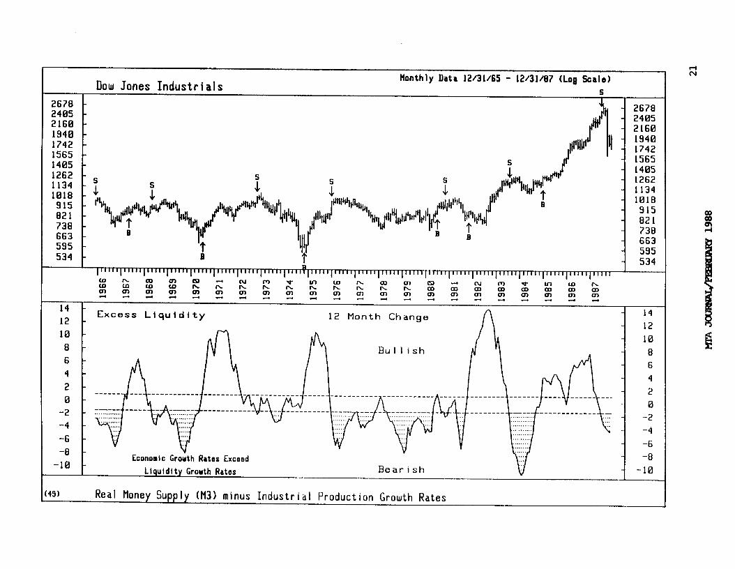
Economic Liquidity

The other category of indicator deals with domestic economic liquidity

16

(chart 49), the liquidity needed to satisfy real growth in the economy. After the economy and inflation ea& absorb liquidity, any excess left over is available to fuel an advance in the financial markets. Our indicator subtracts the annual growth rate of Industrial ProducticPl from the annual growth rate of RealM3. The resulting excess money supply growth is then usd to time the financial markets.

We have found readings above 1.0% have been bullish for stocks, while readings below -1.5% have been bearish. Using these parameters, an investor would have found 92% of his trades profitable and his portfolio would have gained 13.9% per annum versus 2.9% using a buy and hold strategy. The indi- cator turned bearish in July 1987 --catching thecaning crash.

Currently, growth in both tha economy an3 inflation have attained the levels where they typically drain the financial markets. This indicator is warning us that the Fed must ease the monetary reins m or the financial markets may well continue their decline.

Is there any other information we can extract from liquidity indica- tors? Ah yes! We often look to the Mutual Funds Cash to Assets Sector Ratios in aiding our determination of the quality of market leadership (chart 9a). When the cash to assets ratios of sector funds that typically invest in quality issues (e.g. Growth and Growth & Income Funds) are higher than those ratios that typically invest in the lower quality issues (e.g. Aggressive Growth Funds), the market leadership favors quality.

Because the cash to assets ratios of the Growth funds and Growth and Income funds have exceeded, or are closer to, their upper parameters than those of the Aggressive Growth funds, we believe the sector ratios are tell- ing us the long term leadership remains withquality. Nevertheless, the cash to assets ratio of the Aggressive Growth funds increased substantially during the crash. (In fact, switch fund traders who typically invest in the Aggressive Growth funds accounted for 95% of the total $6.4 billion with- drawn from mutual funds during October and November.) We therefore have supporting evidence for short-term strength in the secondary issues (much of which has probably already been fulfilled by the "January effect").

Liquidity indicators can also track the flow between investment vehicles. Chart lla depicts the flow from bond funds into stock funds by dividing the customer purchases of stock funds by the sum of customer pur- chases of stock and bond funds. The trend of this ratio reveals the customers' preference for either vehicle. If the trend is up, the cus- tomers' preference is stock funds; if down, bard funds are preferred. While the recent downturn in this ratio could be expected due to the October panic, a continuation of this trend would be an ominous sign for stocks.

Conclusion

We conclude that liquidity indicators are still valuable market timing tools. It's not that there wasn't a giant sea of liquidity at the time of the crash -- there most certainly was a-~ a nominal dollar basis. But as the

17

market rose it required ever greater amounts of liquidity to produce the same "bang for a buck." ALF detected this divergence and flashed a sell signal. When the Fed reduced the money supply growth while inflation and the economy continued their liquidity demands there was little excess liquidity to keep the financial markets afloat.

At present, (December 1987), our investor liquidity indicators are still bullish. Ard we give them the benefit of the doubt until they produce sell signals. But because real growth in the economy must typically be satisfied before a meaningful long-term bull market is assured, our economic liquidity indicator timpers us from becoming overly optimistic. Until the Fed eases and/or inflation and economic growth moderate, liquidity -- the lifeblood - has the potential to reverse its flow from the financial mar- kets to meet the demands of real economic growth.

Lance J. Stonecypher is a Research Analyst at Ned Davis Research. He is the editor of Industry Watch and the editor of TheEconomic Trend Times, both published by Ned Davis Research. Mr. Stonecypher is a Magna Cum Laude grad- uate of the University of San Diego School of Business.

18

Standard & Poor’s 588 Data 3/31/78 - 12/31/87 Scale) Stock Index tlonthly (Log

323 - 297 - 274 -

rtttt rtt - 323 - 297

252 -

,q-l’ll\rrL t -it

- 274 - 252

232 - 1 232 213 - 213

196 - d +bCr

rrt - 196 188 -

r - 180

166 - Nr - 166 153 - -

140 - 129 +cl t Pb[

tttr

tr WL~tLqJ 153

- 148 -

119 - 109 - rt +’ $’ 1 1.

Vl

-

t t-1 11 [

c t 129

- 119

la0 - clrtl[~Jwt - 189 -

92 - tr 100

92 11111 1,111 1,111 lllll Ill,, ,llI, 1,111 I I I II ,I l I, ,, l l l l

K is ii z l-3 w

0-l z t% 2

m %

OY &

0) M 4

a, 03 In 4 4

80 BB:! -

- 75 (Excluded from Stock Orlsnted Funds ara 80 - %

70 Precious Hetals, Intsrnatlonal - 75

- L Option/Income Funds) - 70 65 - - 65

- 60

- 55

- 50

- 45

- 40

- 35 30 - - 30

- 25 20 - Source: INVESTKNT CoE(pANY INSTITUTE - 20

192 Mutual Fund Customer Purchases of Traditional Stock Oriented

Illa) Funds as a Percentage of al 1 Mutual Fund Purchases

a

20

2678 2405 2160 1940 c 1742 1565 1405 1262 1134 1018

915

flonthly Data 12/31/65 - 12/31/g7 (Log Scale)

s I

Jl - 2670 - 2405 - 2160 - 1940 - 1742

s - 1565 - 1405 - 1262 - 1134 - 1018 - 915 - 821 - 730 - 663 - 595 - 534

Dow Jones Industrials

12 -

10 -

8 -

6 -

4 - 2 -

0 -

-2 -

-4 -

-6 -

-a -

Excess Liquidity 12 Month Change

Bullish

LIi",l"l I li "r"" =-----‘- F--.lth Rates Exceed

Llauldltv _ Growth Rates Bearish

A-l

12

10

8

6

4

2

0 -2

-4

-6 -8

.10

(49) Real Money Supply (M3) minus Industrial Production Growth Rates I

=s i

c s I -4z

1 I

: ~.:.::.:.:::. . :

I:’ :‘; : :‘i’:-.’ : . ,\: . . . I :

F

I I ; i , f ::I I :J I

1960-j-

\ 1961

1962

1963

1964

1965

1966

1967

1969

1969

1970

1971

1972

1973

1974

1975

1976

1977

1978

1979

1990

1981

982

983

984

985

986

987 _

m+ m 2

tm m-+

\

PEA JaJRNAL.- I988

Monthly Data 12/31/65 - 12/31/87 (Log Scale) Standard & Poor ?s 580 Stock Index

324 -

290 - 111’

- 324

259 - JI’ 1

1 ’ - 290

232 -

P

“I~1 It

259

206 - 232

166 - - 206

166 - - 186

149 - p’%$J@ - 166

133 - - 149

119 - ,, ,~#t,/@‘Y1tyt~

- 133

106 - w@+y - 119

95 - fl &ft”tqd+, yf+ + #qrpU”t’~ll~~~’ ,,t, $I Iit’d

v

- 106

85 - t

IzrJ’

95

76 - 65

60 - \lll

76

68

Excess i ve Cash Extreme Pessimism

----mm__-________ --_________-___

----------- ------__--_____ -----------------------------------------------------------

9) Stock Mutual Funds Cash/Assets Ratio Source: INVESTtlENT COtWiNY INSTITUTE

By Ben W. Belch and Arthur T. Dietz

. I. Intmdwtxm

The recent controversy aired in this Journal between Don Dillistone [3] and Norman Fosback [41 concerning Value L!ine's use of the geometric mean in computing indices of growth for equities leads us to believe that now would be a good time to review some properties of means in relation to stock indices. Briefly, the controversy can be summarized as follows: Fosback believes that the geometric mean imparts a "dwnward bias" to an index such as that of Value Line, and Dillistone does not believe that this bias exists. We look at this controversy in retrospect and point out some rather general observations concerning index numbers and averages.

All averages are used in basically two situations: to average data across space (cross-section averaging) and to average data across time (time-series averaging). A stock priceindexinvolves aconsiderationof both types of averaging since it is usual for some measure of return in each time period to be evaluated over time. Both across space and across time a geanetric mean is of interest, but for different reasons in each case.

Consider first the case where avariable is moving across time. For the sake of argument, let us use the population of a mythical country for the years 1960 and 1980 as shown in Figurel. Suppose that it is our task to produce an estimate of the population for the year 1970. If we connect a straight line between the two data points, the value of that straight line opposite 1970 will be the arithmetic mean, X = (3+8)/2=5.5. If on the other hand we fit an exponential growth curve between the two end points [2], then the val e of this curve opposite 1970 will be the geometric mean, G= ((3) (8) ?I2 = 4.9.

Which of these two means offers the superior estimate for 1970? If you have evidence that the growth of population has been arithmetic (such as two hundred thousand persons per year) then the arithmetic mean is the logical choice. On the other hand, if you conclude that the growth has been geometric (such as ten percent per year) then exponential (geometric) growth is a powerful generalization for the growth of populations. The same is true of equity prices as is demonstrated by the wide use of exponential growth charts by security analysts. In view of the fact that stock market analysts think of growth in percentage terms , our choice would be the geometric mean.

In cross-section averaging a major reason for using the geometric mean when dealing with equities is one that is also quite practical. The data shown in Figure 2 illustrate our point and can be replicated very quickly by anyone with a micro-computer at his or her disposal. lb obtain this figure we generated two sets of uniformly distributed random numbers, A and B. There were one-thousand such numbers which ranged from one to one-hundred

24

mA m 1988

for each of the two sets. Next, for each pair of numbers the ratio, R=A,&, was calulated. These ratios can be considered to be the growth relatives for a security where A is the price of the security today and B was the price of the same security in the previous time period. Since A and B can vary between one and me-hundred, they can be thought of as representative of prices actually found in U.S. exchanges for ccxnm~3n stock.

Panel A of Figure 2 shows the frequency distribution of R which is highly skewed to the right as are growth relatives observed in the actual marketplace for common stocks. An easy way to see why these growth rela- tives are skewed to the right is to realize that sinoe the priae of a common stock cannot fall below zero, there is a fundamental asymmetry in the dis- tribution: the ratios seem, so to speak, to pile up against a wall formed by the number zero.

A problem with skewed distributions of this kind is that the arithmetic mean is no longer representative of the data, because the arithmetic mean is easily pulled in the direction of the skewness (in this case to the right). In fact, the arithmetic mean with positive skewness will actually be larger than the majority of the items from which it was calculated. It is for tiis reason that under these conditions statisticians generally substitute a mean which is not so easily pilled in the direction of the skewness. For exam- ple, since incomes are positively skewed, statisticians report the median income rather than the mean income.

For growth relatives , a gccd approach is to take the logs of the data. This operation will cause the distribution to approach symmetry. Just as logarithmetic graph paper tends to spread out smaller values and plsh to- gether larger values, so taking the logs of the growth relatives will pro- duce a distribution like the one shown in PanelB of Figure 2, where the small values are spread out and the large ones are pulled together. This distribution is no longer skewed to any significant extent, and its arith- metic mean is now a representative average for the data. However, the arithmetic mean of the logs of the data is the same as the geometric mean of the original data. Thus, once again the geometric mean is an appropriate measure of the average value of the data.

To be sure there are yet other reasons for using the geometric mean to average growth relatives, but we will not go into them here because they are of a theoretical rather than a practical nature. To read what is perhaps the most famous exposition, see Latane [7].

II. Some vrisons

With this background we are now ready to consider the question of bias for the geometric mean. First, we agree with Dillistone that Fosback's statement that the geometric mean will always be below the arithmetic mean is in error. The correct statement is that the geometric mean can never be larger than the arithmetic mean. This fact has been known since antiquity [9], and holds for positive arguments.

25

However, this formal property of the geometric mean has implications about bias only if we are willing to say that the arithmetic mean is the true mean of the data. We hope that we have dispelled r&ions such as this by now. The arithmetic mean has certain properties ard the geometric mean has others. To say that one mean is true and the other false is quite silly.

There is, however, another problem with the geometric mean that should be mentioned. Dillistone is perfectly correct in pointing out that the geometric mean of growth relatives need r-W be calculated by looking at each relative in a time series, but rather that it can be calculated by using only the two terminal values. He uses this attribute of the geometric mean to counter Fosback's statement that the "error" in the geometric mean is cumulative [4, p. 2941 , a statement which is false but is repeated in at least one other text book [6, p. 541. Nevertheless, the fact that the "cum- ulative error" property of the geometric mean cannot possibly be true has not only been pointed out by Dillistone but was also shown in 1929 by a young Rutgers economist by the name of Arthur Burns [l]. But Burns went further at-d noted a hazard associated with this property: the risk that a poor choice of initial and terminal periods will distort the average in the sense that it will not properly represent the trend in the series.

Three Index Types

Finally, we would like to point out some attributes of three types of indices. These attributes will shed further light on the question of whether the geometric mean index such as Value Line need be lower than some other index of choice.

Let A, and Al be the priceof stock A in period zero (the base period) and period one (the current period) respectively. B. and B

t will denote the

prices for stock B for the same periods. Wa, and Wal wi lbe the weights for A0 and Al and Who and Wbl will be the weights for B. and Bl.

We define three growth indices for these two stocks for two periods:

a. The arithnetic mean of the growth relatives:

This index is a simplified version of E'osback's suggested index.

WqPl (Wbl)Bl +

Wa,) A, mo)Bo I

26

b. The geometric mean of the growth relatives:

This index is a simplified version of the Value Line Index.

IG = ::*b . :;;;;I

C. The value of the portfolio index:

This index is a simplified version of a typical investor's portfolio evaluation.

Wal)/A1 + Wbl)B1

Iv =

(Wa,) A0 + (fio)Bo

Of these three, McIntyre argued many years ago that index c. was the index that the typical investor was interested in, where the weights QI the stocks were the exact number of shares that the investor carried in his or her portfolio [8]. Of course, since no general stock index can be calcu- lated with these weights, some compromise set of weights must be substi- tuted. We mw examine two of these compromises.

If one takes the weights to be all equal to one (as does Value Line) then we have what is generally (but incorrectly) called the case of unweighted averages. On the other hand,

In this case, while lG can never be greater than Iv if we follow Dillistone's technique of causing the pro-

portion of the value in the portfolio accounted for by securities A and B to be the same in each of the two time periods, then all three indices give identical indications of growth.

The proof is simple. Let Po and Pl be the value of the portfolio in the base and given periods respectively. Then

(Wao)Ao = (Wbo)Bo = Pd2

(Wq)Al = (Wbl)Bl = Pl/2

27

Therefore

IG =

Iv =

= q/p,

.

i P1/2 y2 - +

III. Conclusions

The choice of an ideal stock index is one which has bothered mankind for many years. The reason is that the criteria for acceptance are neces- sarily subjective. What we have tri& to show is that the Value Line Index cannot be said to be biased in any particular direction. It simply measures attributes of stock growth which are different from those measured by an arithmetic index.

Ben W. Belch is Professor of Economics at Rhodes College and President of the Belch Group, Inc. His academic specialties are statistics and econo- metrics.

Arthur T. Dietz is Mills Bee Lane Professor of Finance at Emory University. He has been an officer and Trustee of the Atlanta Society of Financial Analysts, and arrently manages two option funds and serves as a Director of Alpha Fund.

28 KI!A m 1988

Figure 1 -- Population in 1960 and 1980, Mythical Country, a rd TlVo Estimates for 1970 (millions)

2

t

I

I

I I )

1960 1970 1980

29

Figure 2 -- Skewness Reduction by Logarithmic Transformation

f req, % f req, %

100

80

Panel a,R

60

40

20

JR JR 0 20 40 60 80

freq,% /r

50

t Panel b)Ln (R)

A0 -

' >Ln(R) -5 -4 -3 -2 -1 0 1 2 3 4 5

30

1.

2.

3.

4.

5.

6. Khoury, S. J. Investment Management, MacMillan, 1983.

7. Latanc, Henry. "Criteria for Choice Among Risky Ventures," Journal of Political Economy, 1959, 114-155.

8.

9.

Burns, Arthur F. "The Geanetric Mean of Percentages," Journal of the American Statistical Association, 1929, 296-300.

Croxton, F.E., Cowden, D.J. and Belch, B.W. Practical Business Statistics, 4th ed., Prentice-Hall, 1969.

Dillistone, Don. "The Value Line Myth," MIA Journal, Feb., 1986, 21-30.

Fosback, Norman. Stock Market Magic. The Institute for Econometric Research, 1976.

Realities," MIA Journal, Feb.; "Geanetric Means - Old Myths and Old

1987, 72-75.

McIntyre, Francis. "The Problem of the Stock Price Index Number," Journal of the American Statistical Association, 1938, 557-563.

Siegel, Irving. Agg egation and Averaging WE. Upjon Institute for Employment Research:1968.

31 KI'A m 1988

On the Measurement of Price Velocity

Richard C. Orr, Ph.D.

Introduction.

Of all the tools used in technical analysis, the most common after the trend line is probably

the moving average. Buy or sell strategies which are triggered by the movement of price above

or below a given moving average or by the movement of a shorter-term moving average above a

longer-term moving average have been used for decades. A more general process involves

studying the ratio of two moving averages over a whole range of values. While we realize that,

to many technicians, this idea in itself is not a new one, we intend to take it one step further.

It is possible to write a formula which will transform any ratio of two moving averages into

a rate of return. This will allow the user to deterrnine the growth rate of prices from any time

frame, thereby expanding his or her perspective of price behavior into another dimension. The

name we have given to this new function is price velocity. While this transformation lends itself

to calculation by computer, it can also be carried out with a hand-held calculator or even pencil

and paper. Calculation of the ratio requires seven arithmetic steps, the transformation requires

only an additional five steps.

The purpose of this paper is to acquaint the reader with the idea of price velocity and its

computation, as well as to look at a few ways in which it is used. Although in the process of

discussing price velocity we will use specific examples as illustrations, it is not our intention to

suggest that these even begin to characterize the scope of this area.

32

Calculation of Exponential Moving Averages.

Unlike arithmetic moving averages, exponential moving averages are simpler to calculate,

require the storage of much less data and provide for the influence of a given piece of data to

decay over time, rather than to carry its full weight one day and no weight for the next*. If we

choose a rate of decay, l-A, where A must be positive, but can be as large as one, the

exponential moving average, M, with that particular decay rate is calculated as follows for a new

price, P:

M current = (l-A)Mlag + A*Pcment

The price data could be obtained at any rime interval: hourly, daily, weekly, or some other

period. The behavior of this moving average over time depends then on two factors: the rate of

decay of the data and the frequency of the data. As the decay rate gets closer to 1, the smoothing

process slows and the moving average becomes longer-term. At the other extreme, if 1-A = 0

then the moving average is just price itself, which corresponds to a one period arithmetic moving

average, the fastest that exists.

Notation.

Although any rate of decay between zero and one may be used, we will restrict the

examples in this paper to five exponential smooths. Decay rates in other areas such as physics

are often stated in terms of half-lives. The half-life of a substance is the amount of time

necessary for one-half of it to decay. In a similar fashion, we can talk about the number of

periods (hours, days, weeks, etc.) it takes for our data to have one-half the influence it did

originally. Suppose we focus for the time being on daily data. The following table gives both

the exponential smoothing functions and notation we will use for each half-life.

* For a more detailed comparison of these two smoothing techniques, see “The Use of Volume As An Early Warning Signal”, Market Technicians Association Journal, (15) May 1983

33

Half-Life Formula

0 M, urrent = pcurrent 1 M, urrent = J”last +Jpcurrent 2 M, urrent = .707Mlast +.293Pcment

4 M, went = .841Mlast +.159Pcment

8 M, urrent = .917Mlast +.083Pc,ent

16 Marrent = J58Wast +-w2Pcurrent

TABLE 1.

Notation

Smg

sm1

sm2

==I

sm8

sm16

The larger the half-life, the slower the smoothing process, so of the above exponential smooths, sm16 is the slowest. We have found that in all our work it is sufficient to consider

only exponential moving averages which have half-lives which are powers of two. However,

the reader should feel free to experiment with any other exponential moving average.

The Ratio of Two Moving Averages.

In order to get a feel for the rate of growth (positive or negative) of prices it is necessary to

look at two moving averages. Remember that since price itself is a special case of a moving average (SW), looking at price itself together with any other moving average would also work.

Now, given two moving averages we consider the ratio of the faster moving average to the

slower moving average. This ratio has the flavor of price velocity:

l The larger the ratio, the higher the faster moving average is above the slower moving

average, and the faster the rate pf increase of prices.

l The smaller the ratio, the lower the faster moving average is below the slower moving

average and the faster the rate of decrease of prices.

l The closer the ratio is to one, the closer the two moving averages are to each other and

the closer the sequence of prices is to being constant.

34

The “chart” on the following page illustrates the above property for the ratio sml/smz. Prices

will start at 100, increase at one percent per day, level off, decrease at two percent per day and

level off again. Note how the ratio tends to home in on constant value if the growth rate is

uniform for a while.

The Transformation to Price Velocity

Although the ratio of two moving averages appears to have the flavor of growth rates,

growing or shrinking as prices advance or decline, the implicit growth rates just cannot be read

from the ratio. With daily data we would like a ratio of 1.01 to reflect an increase of one percent

per day in prices. With weekly data we would like a ratio of .98 to reflect a decrease of two

percent per week in prices. If the moving averages are arithmetic then there is no clean

transformation. This should not be surprising since growth rates are an exponential property.

If, however, the moving averages are exponential, then a fairly simple transformation exists:

Given two exponentially smoothed moving averages:

FAST: MF with decay rate l-F, and

SLOW: MS with decay rate l-S,

if prices grow at a constant rate r then the quotient Q MF = - will approach the value

F(l-S-r) MS S(l-F-r) *

The reader is spared the proof of this result. However, for completeness it has been placed in the

Appendix. If Q has the form above then by simple algebra we can solve for r as follows:

F( 1-S-r) Q=S(l-F-r)

QS-QSF-QSr = F-FS-Fr

r(F-QS) = F-FS-QS+QSF

r _ F(l-S)-SU-F)Q . F-SQ

35

KIT4 JOURNAT- 1988

---B-B-

. . . . . . . . . . . . . . . .

But r is the rate at which prices are growing and therefore price velocity, which is the rate of

change of prices from the time perspective of whatever two moving averages are being used, is

given by:

pv = r = FU-S)-S(WQ .

F-SQ

The only variable in this function is Q, the quotient.

Example: Suppose the decay rate for MF = .91, while the decay rate for MS= .97. A growth rate for

prices of r = 1.01 means that the ratio

MF Q= E will tend toward

.09(.97-1.01) .03(.91-1.01) = l-2,

so the faster moving average should be 20 percent above the slower moving average.

Conversely, if the ratio of these two moving averages is 1.2, then solving for price velocity, PV,

in the above formula, we get:

pv = (.09)(.97)-(.03)(.91)(1.2) _ .05454 _ 1 .09-(.03)( 1.2)

o1 .054 -

which, of course, is the rate we would want to get.

In the following table are listed values of price, moving averages, their ratio, and the

associated price velocity on four different days taken from a sequence of fifty prices, given MF

different growth rates and moving averages. The limit ratio is the value toward which - MS will

tend. Note that PV approaches the given growth rate.

37

Kt!A m 1988

TABLE 2.

INITIAL PRICE: 20 GROWTH RATE: 1 .OOl F = .500

s = .293

JJMIT RATIO: 1.00141

INITIAL PRICE: 20 GROWTH RATE: 1 .OOl F = .159

S = .083

LIMIT RATIO: 1 .OOS72

NTIAL PRICE: 20 GROWTH RATE: 1 .OOl F = 1.000

s = .042

LTMIT RATIO: 1.02279

INITIAL PRICE: 20 GROWTH RATE: 1.003 F = .159

S = .083

LIMIT RATIO: I .02247

Ih’rTIAL PRICE: 100 GROWTH RATE: .992 F = .500

s = .293

LTMIT RATIO: .9885 12

PRICE

.MF MS MF MS PV

PRICE

MF MS MF MS PV

PRICE

MF MS MF MS PV

PRICE

hlF

MS MF

MS PV

PRICE

MF MS MF MS PV

DAY 1 DAY 10 DAY 25 DAY 50

20.04 20.22 11 20.5266 21.046 20.02 20.2009 20.506 1 21.025 20.0117 20.1734 20.4772 20.9954

1.00041 1.00137 1.00141 1.00141

1.00029 1 a0097 1.001 1.001

20.04 20.22 11

20.0064 20.1299 20.0033 20.0838

1.00015 1.00229

1 .oooO? 1.0004

20.5266 21.046

20.4198 21.9354 20.3252 20.8188

1.00465 1.00560

I .0008 1 1.00098

20.04 20.22 11 20.5266 21.046

20.04 20.22 11 20.5266 21.046 20.0017 20.048 20.215 20.6269

1.00192 1.00864 1.01541 1.02032

I.00008 1.00038 1.00068 1.00089

20.1603 20.8978 22.1874 24.5159

20.0255 20.5257 21.7339 24.0100 20.0133 20.339 21.3398 23.4924

1.00061 1.00918 1.01847 1.02203

1.00011 1.00161 1.00327 1.00392

98.4064 91.5437 81.1528 66.3888

99.2032 92.2879 81.8125 66.9286 99.533 1 93.324 82.763 1 67.7063

.996686 .988899 .988515 .988512

.997665 .992265 .992002 .992

PfA JCv 1988

Notation for Charts.

On the next four pages are charts of the SP500 index for the years 1977 and 1987, together

with the graphs of certain price velocity functions. In order to specify which PV we are using, sma

let PVa;b denote the price velocity associated with the quotient Qab = q br the examples we

have chosen:

PVl;2 = (.soo)(.707)-(.293)(.500)41;2

SOO-.293Q1;2

.354-.146Ql,2 sm1 = .5()@2g3Q1,2 ‘where Q1;2 =- sm2 ’

PV4;8 = (.159)(.917)-(.083)(.841)Q4;8

.159-.083Q4,8

.146-.07oQ4,$ sm4 = .159-.083Q4;8

, where 44;~ = smg , and

PVO;16 = (1)(.958>-(.042>(O>Qo;l6

l-.04240;16

.958 = l-.04240,16 ’

where QO;l6 =s.

Also, in order to read the values more easily on the graphs, we have converted the values of PV by using the formula PVa;b = lOO,OOO(PV-1). Under this conversion PV = 1.001

becomes +lOO, while PV = 1.0005 becomes +50 and PV = 0.998 becomes -200.

39

Km JUJV I.988

Observations.

A number of points of interest can be found in the charts on the previous four pages.

l The level of volatility of the market dramatically changes the range of values for price

velocity. Note that using .the same scale for both 1977 and 1987 we have much larger

values for all three PVs in 1987.

l The function PV1;2 is clearly more sensitive to change than either PVq,8 or PVo;16.

Since the exponential smooths are both fast, the time perspective is very short-term.

l The function Pv(); 16 iS a SOI? of hybrid betWeal Pv1;2 and Pvq$. The geneId level Of

values of PVO; 16 seems to follow those of PV4;8 pretty closely, but the changes from

increasing to decreasing of PVO;16 actually correspond more closely to those of PV1;2.

l In a flat to slightly down-trending market like 1977, values of PV4;8 or PVO;16 rarely

get very positive. Even with small positive values for these functions one might maintain a

short position because the average growth rate would still be rather small. This point of view helps combat whipsaws. In 1977, PVO; 16 remained under 100 after the first day,

while it crossed back and forth over 0 nine times.

l Large gains or losses in the market cannot occur while values of PV4;8 or PVo, 16

remain close to 0. For this reason one could create a neutral strip on either side of 0, say

- 100 < PV < + 100, which could be used to separate strongly trending markets from fairly

trendless markets. This would have been helpful in determining the major moves which

occurred in the 1987 market.

Summary.

In this paper we have taken the reader through a step-by-step development of the notion of

price velocity. We now can see that the actual value which is calculated for price velocity

depends not only on the price series used, but also on the two moving averages which give us a

frame of reference for measuring the change in price. The emphasis has been placed on the

careful development of a new tool, rather than on the compilation of favorite strategies using this

tool. Price velocity lends itself not only to trend following strategies, but overbought/oversold

strategies, market volatility measures and some cyclical investigations, just to mention a few.

44

Appendix.

Theorem. Consider the following price series with initial price, P, and growth rate, r:

P, Pr, Pr2;..,Prn,-.-.

If

MF*> M+ MF~~-, MF,,-*

and

Msov Msl, Ms2,-, MS,,-

are the corresponding exponential moving averages with decay rates 1-F and 1-S respectively,

where 0 5 1-F < 1-S < r, then

MFn n%%oMS,=

F(l-S-r) S(l-F-r) ’

Proof:

MFo=P

MF 1 = (1 -F)P+FPr

hIF-, = (1 -F)zP+( 1 -F)Pr+FP?

hlF n = (1 -F)nP+( 1 -F)n- lFPr+...+( 1 -F)Prn- l+FPrn

= (l-F)nP-PF( 1 -F)n-tPF( 1 -F)n+( 1 -F)n-lFPr+...+( 1 -F)Prnml +FPrn

= P(1-F)n(l-F)+PF((l-F)n+(1-F)n-1r+...+(l-F)rn-1+rn)

= p(l.F)n+l+pF((l-F)~~~l~rn+l) .

Similarly, h?S, = P( 1 -S)“+l +PS( (l-s)n+l-rn+l

> 1-S-r *

45

Hence

MF~ P(l-F)n+l+pF(‘l‘F:“+~rn’l) - - MS,=

*

Dividing both numerator and denominator by Prn+l, we have:

MFn (e)n+l+&((F)n+l-l)

Finally, since 0 5 1-S < I-F < r, we have

F(l-S-r) = S(l-F-r) ’

Dick 0x-r is Vice President for Research at John Gutman Investments Corporation and an

Associate Editor of the hlarket Technicians Association Journal.

46

TURNING POINTS FOLLOWING M AND W WAVES Arthur A.Merrill 03 18 87

This is another investigation of the relative bullishness or bearishness of the five turning point waves that I have classified as 16 M and 16 W waves.

The question I put to my computer was this: look at the four turning points which follow each M or W wave. Where were they located relative to the five points in the M or W wave? Were they higher than any of the points in the M or W? Were they lower ? Where were they in between?

For example, consider an Ml3 (a triangle):

w-. --w-w

:P

y. - - - - - -

-- - --

NW - -qy&-igy- z . -- -w----w.-

2 0 WLI -es MB ---a

1

The dashed lines are set by the five turning points in the M13. The numbers identify six possible areas. If a following turning point fell in area 6, for example, it would be higher than any of the points in the M13. In the example, the four following turning points were located in areas 6,3,4, and 2.

I asked the computer to look at the Dow, for which I have located 745 turning points (5% filter) since March 1898. It sorted out the M and W wave classes, and looked at the four turning points which followed each wave.

For example, here is the score for the M13:

5 1 0 2 1 4 2 3 2 2 3 0 1 0 0 2 0 2 0 2 1 0 2 1 3 Avg. 5.6 3.8 5.1 3.7

The first turning point was found nine times in area 6, once in area 5, and twice in area 4. The average for the first following turning point was 5.6 .

I then asked the computer to rank the various M wave averages from 1 for the most bullish down to 16 for the most bearish; and then to do the same for the 16 W waves. The result is in the table which follows. The right hand column was obtained by totalling the four ranks and then ranking the totals. I have transferred the right hand column numbers to the chart of wave shapes; it is the circled number on each chart.

Conclusion: Ml 1 is the most bullish (rank one) of the M waves; M3 is the most bearish (rank 16). W16 is the most bullish of the W waves; W6 is the most bearish.

47

Turning Point: 1 2 3 4

Ml 13 11 15 14 13 M2 11 13 11 16 12 M3 16 15 14 12 16 M4 7 8 6 7 7 M3 15 16 16 10 15 M6 8 4 4 11 6 M7 12 12 10 13 11 M8 5 7 3 5 4 M9 14 14 13 15 14 Ml0 6 6 8 9 8 Ml1 2 1 1 1 1 Ml2 9 10 12 6 10 Ml3 3 3 5 3 3 Ml4 10 9 9 8 9 Ml5 4 5 7 4 5 Ml6 1 2 2 2 2

WI 11 13 16 16 15 w2 12 14 14 14 14 w3 9 11 9 12 10 u’4 15 10 12 6 II w5 8 8 8 11 8 W6 13 15 15 15 16 w7 14 16 11 10 12 W8 4 4 2 1 2 W9 16 12 13 13 13 WlO 3 5 5 3 3 WI1 7 1 7 4 5 W12 5 7 6 5 7 w13 10 9 10 9 9 WI4 2 6 3 7 4 W15 6 3 4 8 6 WI6 1 2 1 2 1

48

KCA JWRNt&&)BUmRY 1988

MI

0 I3 r ‘G\ 2 I 4 3 5

M2

2 1534 ( 3 1 M5 I5 4

I M6

32415 3 2 5 I 4

M9

14 I!5 4 2 3 I 5 4 25 I3 4 3 5 I 2

Ml3 Ml4 Ml5 I Ml6

0 3

i\% d 5 I 4 2 3 523 14

b 31425

-+J h 4 I 3 2 5

I 4 ,

I MI0 I I MII

1 I 1

0 9

rs\

J

5 2 4 I 3

3 I5 2’4

MB

4 I 5 2 3

Ml2

IO

~ 5 1324

1

53412

KFA Jv 1988 49

0 15

\2i 13254

yq pJ=q

I * 2 5 3 14352 I 5 2 4 3

I 5 3 4 2 23154 24 I53 243 5 I

c

:

w9

0 I3

ib

25143

WI3

0 9

\I\/ 35142

WI0 0 3

\rl 2534 I

WI4

0 4

d 3524 I

WII

0 5

a 3 4 I 5 2

w.r 5

4 5 I 3 2

WI2

0 7

d 3425 I

r

WI6

4523 I

50 IWA m I.988

MERRILL ANALYSIS INC.

bx 228, chqpoqw, NY 10514

INTRADAY VOLATILITY

In a paper presented at the MTA seminar in May, Jack Schwager demonstrated that volatility, measured by day-to-day change, hasn’t increased in recent years.

When I returned home from the seminar, I asked my computer to look into our hourly data bank, and check the intraday volatility.

The results are shoun in the two charts. The top chart shows the average hourly change in the Dow Industrials in each quarter. The recent volatility appears rather modest when compared with the volatility experienced in 1974. The regression Line, however, does show a mild upward trend.

The Dow industrials are charted as a dotted line.It appears that you would have usually done quite well if you bought equities whenever the volatility shot through the roof.

The lower chart notes extremes in hourly activity. The highest percent in each quarter is charted, rather than the average. The two charts are quite different. In some years, the average was high, but the extremes were moderate; in other years the average was IOU,, but some extremely high hourly changes appeared. The highest change the computer found was on March 27,19SG, when the Dow rose 2.76% from 739.59 at 3 PM to 759.98 at the close.

(Notes: The year 1985 has inexplicably vanished from our data bank; this year was omitted in the study. Six hourly changes were calculated each day, &ginning with the change from the opening to IIAM and ending with the change from 3 PM to the closing bell. When the market started the 9:3G AM opening, the first change of the day was measured from 1G AM to 11 AM.)

Arthur.A.Merrill Merrill Analysis Inc. 05 15 87 file VOLl:l (F)

51

HOURLY PERCENT SWING

Ih EPCW QUARTER Ih EPCW QUARTER (DJ INDUSTRIALS) (DJ INDUSTRIALS)

i

/

1 I I I I

INTRADAY VOLATILITY 1

HIGHEST PERCENT C”AiGL MADE IN ONE HOUR IN EACH QUARTER IDJ INDUSTRIALS) I :

.‘. : i _!,.‘.,,. ., ; .. . . .

: .” ._ :’ : :

/

- :

: MERRILL AMALTS

:: 03lS87 0

197.2 1973 1974 197: ,,I ,L,II’L

1976 IS77 Is78 1975 I9EC lS8C 1982 1983 I984 1985 1906 l98i

52 KI'A m 1988

Demand slacks off and supply increases if growth is slowing down. We , as technicians, can sometimes detect this in advance from the price curve. Compare the earnings curves of CPF, RAL and RBK, which seen to be leveling off, with those of CPQ, EBF and GE, which have been accelerating.

Demand slacks off and supply increases when prices appear expensive. This component of demand picks up if prices appear to be bargains. The most popular yardstick for expensiveness is the P/E ratio, which is easily noted with the proposed chart form. Compare CPQ and CFA, which are relatively expensive at 25, with TTC and RAL at 13. The price curve of RBK may appear inflated, but it is still at the relatively modest level of 15.

Growth sometimes stimulates demand to the degree that a higher P/E appears justified. Note CPQ and CFA, where prices have been pushing upward through one earnings curve after another. On the other hand, note CAR, which has been falling behind.

Conclusion: the proposed price/earnings chart adds another dimension to our analyses.

AAM : 090287 PE2/SCR(F)

53

PRICE/EARNINGS CHARTS: Arthur A.Metrill

Technicians have learned that future earnings prospects are discounted in advance by prices. We focus our attention on prices, and usually leave the earnings data to the Fundamentalist. However, we, as Technicians, are concerned with supply and demand. Since the demand for stock by a large group of investors is definitely influenced by earnings performance, shouldn’t we, as technicians, include earnings in our analyses?

A single earnings curve is included in many of the published price charts. This paper proposes that earnings be included as a family of curves. Each curve in the series would chart the earnings for the preceding year multiplied by a factor, such as 10,15, or 20.

Note the simplicity of interpretation. When the price curve crosses the EPSxJO line, the stock is being priced at a P/E of 10. If it moves up to the EPSxlS line, it is now priced at a P/E of 15.

In the examples of this paper, a filtered price wave is used. Swings of less than 10% are ignored. M and W waves can easily be classified. However, if you prefer a bar chart, it could be substituted. A volume curve could be added if you wish.

The examples use the logarithmic vertical scale, which is proper if charts are to be co’mpared. Rates of change of price and volume are made evident by this scale, and trend lines become valid.

Note that all of our usual technical tools can be applied to the price curve. These include trend lines, support and resistance, moving averages, wave patterns and the rest.

In addition, this chart answers a Jot of questions.

There is a demand for the stocks of growing companies. Is this a growth company, or has it matured? Compare the

slope of the earnings curves of CPQ with those of GE. CPQ can certainly be labeled a growth company; GE is mature.

54

: ,. 0 i Lo -‘P

: soi-

,-is ; :

r COMPAQ COMPUTER ! : : CPQ

t : r ,

40.

1 EPSX30fl .’ ,_/ .’ i i

250 / j CAR /

I I A 1 i

b---- I

,5ot-*---- ./--.? I

~251:~ .‘.‘, !

R ,_. ..” I I

/

/J F M nn J J A 5 0 NO JFY91MJJnsoNo’

(IV66 1967

/ _ CoMPyrER FACTOR” I I CFA

I 30

: ,b ,..... ..-I

t :.’ /̂ I .I. I I

20' 1

: : : I/

30

so, t ! ENNIS BUSINESS FORMS

/ EBF 1 I

40’ L I I I I I

r I I

-- - I I I .I:....- I I I

‘O,,. A.y J J. J&8 8.8

1986 I IS87

I

1966 1987

55 Kt!A Jv 1988

I Y 120, i ..__.. ..I. a,.. __.. g . . . . . . ..j.J

50. I I m / “1,

r i I.-, ...L-...

..’ ..‘b _.’

: .._.._,. l... ,

lb./ ‘QJJ ;

I Xl:

40

4 : . .

REESC* _’ 6OL :’

,:’

k : p.’ / ..’ $

t : , I..' I

RBK

ISO I /

140. 4

r RALSTON P”RlNA

_._.... . ...“” : RAL-

Ia0 I I :

I20 I EPSix+..

t i / :’ IlOt / 1 I

.t’

I I I I

i . . . .._... . ...“..

I : :

1986 1967

50. E TORO tn /_

i I

40‘ /

56

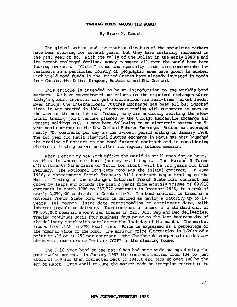
By Bruce M. Kamich

The globalization and internationalization of the securities markets have been evolving for several years, but they have certainly increased in the past year or so. With the rally of the Dollar in the early 1980's and its recent prolonged decline, money managers all over the world have been looking overseas. "Global" funds and specialty funds that concentrate in- vestments in a particular country or geographic area have grown in number. High yield bond funds in the United States have already invested in bonds from Canada, the United Kingdom, Australia and New Zealand.

This article is intended to be an introduction to the world's bond markets. We have concentrated our efforts on the organized exchanges where today's global investor can get information via real-time market feeds. Even though the International Futures Exchange has been all but ignored since it was started in 1984, electronic trading with mmputers is seen as the wave of the near future. Indeed, many are anxiously awaiting the elec- tronic trading joint venture planned by the- Chicago Mercantile Exchange and Reuters Holdings PLC. I have been following on an electronic system the !5- year bard contract on the New Zealand Futures Exchange. Volume has averaged nearly 700 contracts per day in the 3-month period ending in January 1988. The two year old Matif financial futures exchange in Paris has just launched the trading of options on the bond futures' contract and is considering electronic trading before and after its regular futures session.

When I enter my New York office the Matif is still open for,an hour, so this is where our bond journey will begin. The Marche a Terme d'Instruments Financiers or Matif for short, will be two years old this February. The Notionnel long-term bard was the initial contract. InJune 1986, a three-month French Treasury Bill contract began trading on the Matif. Trading in the exchange's Notionnel French State bond contract has grown by leaps and bounds the past 2 years from monthly volume of 69,918 contracts in March 1986 to 357,777 contracts in December 1986, to a peak of nearly 2,250,OOO contracts in October 1987. The bond contract is based QI a notional French State bond which is defined as having a maturity up to lo- years, 10% coupon, issue date corresponding to settlement date, with interest payable cn delivery. Each contract is issued in astandard unit of FF 500,000 nominalamountand trades in Mar, Jun, Sep and Dee deliveries. Trading continues until four business days prior to the last business day of the delivery month with settlement the last day of the month. The market trades from 1OAM to 3PM local time. Price is expressed as a percentage of the nominal value of the bond. The minimum price fluctuation is 1/2Oth of a point or .05 or FF 250 per contract. The Chambre de compensation des in- struments financiers de Paris or CCIFP is the clearing house.

The -/-lo-year bond on the Matif has had some wide swings during the past twelve months. In January 1987 the contract rallied from 104 to just short of 109 and then corrected back to 104.50 and back up over 108 by the end of March. From April to June the market made an irregular correctian to

57

102. This was followedbyamid-summer bounce to 104.50 and thena steep plunge to 86 by October. Since the October 1987 low, the market has recouped much of the 1987 loss and is currently trading in the 99 to 102 range.

Travelling to Amsterdam to continue our journey to trade b01&, we find the European Options Exchange (EOE) ard the Amsterdam Financial Futures Mar- ket. The EOE has a new trading floor and computer system with plenty of capacity to handle their bond option. Options are listed in three expira- tion months, e.g. February, May and August. The exercise price is quoted at a percentage of the nominal value. Trading ends on the third Friday of the expiration month. The Amsterdam Financial Futures Market launched trading in theirguilder bond futuresonJune19, but do not have any data on this contract at present.

Moving on to Stockholm, the Stockholm Options Market (OM) was estab- lished inJune 1985 and started trading in interest rate options in March 1986. The Swedish Options and Futures Exchange (SOFE) opened cn March 13, 1987 and has plans to compete with the OM with their own interest rate fu- tures and options. Though the OM and the SOFE seem to have volume of 15,000 to 25,000 contracts per day, we have not seen a breakout IX see how mu& of the volume is interest rate related. Before leaving the continent we should mention that the Swiss Options and Financial Futures Exchange (SOFFEX) is scheduled to open on March lof this year. Even though the exchange is a result of the efforts of the stock exchanges in Zurich, Geneva and Base1 and the five major banks, the exchange may eventually trade financial futures.

Making the jump over to the City or London, we find the London Inter- national Financial Futures Exchange (LIFFE). The financial community there can now trade long, medium and short Gilts, a Japanese Government Bard ~XI- tract, Eurodollars and the US Treasury Bond contract, The volume of trading in the Long Gilt has improved from 311,917 contracts traded in December 1986 to approximately 350,000 contracts traded in December 1987. Currently, open interest in Iong Gilts is in the vicinity of 25,000 antracts, close to the average daily volume. The options on the Long Gilt contract have shown spotty activity with an average of approximately 3,000 to 4,000 contracts being traded each day (calls plus puts) between October 1987 and January 1988. The vast majority ofoptionvolume has been calls. LIFFE has made links to other exchanges and have expanded with a Yenbond contract and a CBOTboxd contract. More recently, the Medium Gilt contract was introduced. The Long Gilt future trades from 9:OOAM to 4:15PM, local time. The Short Gilt future starts ax-d stops trading five minutes later than the Iong Gilt.

The Long Gilt Future trades in units of L50,OOO (Sterling) nominal value notional gilt with a12% coupon. Delivery may be made of any gilt with 15-25 years to maturity as listed by LIFFE. Delivery may occur cn any business day in the delivery month. Like other bond contracts, March, June, September and December are the delivery months. Last tradingdayistwo business days prior to the last business day in the delivery month. 1/32nd is the mininun price movement and has a value of L15.625 (Sterling).

The option on the Long Gilt Future calls for trading in one long gilt

58

futures contract. Ihe same delivery months are traded and exercise can be done on any business day until 5:OOPM The options trade in multiples of l/64 (L7.8125 Sterling) and strikes go up (and down) by 64/32nds from 118 to 120 to122, etc. Trading in the options starts two minutes after gilt fu- tures begin, but they halt trading at the same time as the underlying future. Gilt options cease trading, six business days prior to the first delivery day of the Long Gilt Futures contract.

The Short Gilt Future is twice the size of the Long Gilt-- LlOO,OOO Sterling nominal value Notionnelgilt with a 10% coupon. Delivery may be made of any gilt with 3-4-l/2 years to maturity as listed by LIFFE. The minimum price movement is 1/64th and has a value of L15.625 (Sterling).

Likethebond market in Paris, the Long Gilt Future has seen several big swings. During 1986 the Iong Gilt rallied from 110 at the beginning of the year to 130 in April and then had three legs down, bringing prices to under the 106 level in November. By May-June 1987, Gilt futures were back upto127-16 before they came under selling pressure again. This decline ended in October 1987 in the 111-110 area. Since the October low, Gilts have traded sideways in a ten point band from 115 to 125. We would look for the Iong Gilt continue to trade sideways to higher for several more months.

Going across the Atlantic we fird several futures contracts, besides the major ones in Chicago, getting our attention. In Canada the Toronto Fu- tures Exchange (TFE) and the Montreal Exchange see virtually all the volume in bond options. The TFE has a struggling Canadian T-Bond and T-Bill futures contract and an option on government treasury bonds. The lion's share of the interest rate option volume seems to go to the Montreal Exchange. Trading is carried on by speculators and professionals. Supposedly, most of the hedging is done against mortgage-backed issues. We have no figures, but many Canadians probably cross-hedge into the more liquid Chicago markets. A Canadian bond future could eventually be launched in Chicago. TheLong Government Bond Future on the TFE has $100,000 face value and is based on a 9% coupon Government of Canada Bonds which do not mature and are not callable for at least 18 years from date of delivery. The contract months are March, June, September and December and trading hours are 9:OOAM to 3:15PM. Prices are quoted on a percentage of par basis in increments of thirty-seconds, e.g. 78-12/32. The TFEbond optionhas a trading unit of $25,000 face value ard trades until 4:OOPM. Exercise prices are set to bracket the current market price of the underlying bond at inter- vals of 2.5 points.

We have been charting the cash Canadian 10-l/4% Bard of 2004 since the beginning of 1987. From January 1987 until last October this issue had traded in a very well defined downward sloping cfiannel from 115 to 94. Like the other bond markets that witnessed strong October-November rallies, the lo-1/4%s has rallied back to the 107-108 area. We have longer termprice objectives that measure up to the 113 level.

Coming down to New York City, the Financial Instrument Exchange or FINEX (a division of the New YorkCottonExchange) has been trading a Five Year U.S. Treasury Note futures contract since May 1987. Between November

59

1987 and January 1988, average daily volume was approximately 2,200 con- tracts. Open interest is now up to 7,500, but has been quite volatile the past six months with swings between 3,000 and 8,000 contracts. Trading is from 9:OOAM to 3:OOPM New York Time. The trading unit is $100,000 face value of U.S. Treasury notes including the current five year treasury note axrl three previously issued five year notes. Like all the other contracts in the States, the delivery months are March, June, September and December. The minimum fluctuation is one half of 1/32nd of 1 point ($15.625 per con- tract). The daily bar charton the Five Year Bond has not been a mirror of the other contracts in Chicago, but rather has traced out its own "cleaner looking" patterns. (The CBT Notes and Munis have at times given signals before the T-Bond antact. Traders could watch the Five Year Note for early signals as well.) After plunging to under 91-00 during the October 1987 market low, the Five Year Note ralli& to 97-08 ati then traded sideways to higher throughout November, December and most of January. It appears that market has started another leg up from 97-08 that could meet resistance in the 100-16 to 101-00 area.

Because T-Bond futures a-~ the Chicago Board of Trade lead the industry in volume and open interest , we assume most people in the industry area already well versed in the contract specifications. We would like to briefly menticn the T-Bond contract on the MidAmerica Commodity Exchange which is an affiliate of the Chicago Board of Trade. The contract is half- sized with a trading unit of $50,000 faoa value of U.S. Treasury bonds. The trading hours are interesting and useful in that they extend from 7:2OAM to 3:lSPM Chicago time. This can allow you time to reduce or add ti a position before news releases or just to get an indication where the market is trading. Trading in this smaller contract is mostly speculative, so a tech- nical analyst might consider comparing the volume on the MidAm to the CBOI to get an index of speculation, like equity technicians comparing the Ameri- can Stock Exchange to the New York Stock Exchange.

Moving West to the Far East we can stop at the Tokyo Stock Exchange to trade the Yen Bard Futures contract. Yen Bond Futures trading has grown im- mensely since it began in October 1985. With a very strong Yen and a government that lowered interest rates the first half of 1986, many institu- tional investors such as banks and life insurance companies turned to the Yen Bond contract for asset hedging. The market rallied cn volume exceeding 100,000 contracts U-I many days and monthly volume exceeded 2 million eon- tracts during March 1987. The excitement of the marketplace also swept up individual speculators and even some manufacturing firms before a steep downward correction began in April 1987. Like other futures contracts, the YenBond contract is not based on the future price of an actual long term government bond. The contract describes a unit of 100 million Yen based on a price index with a coupcn rate of 6% and a lo-year maturity. The contract trades from 9:00 to 1l:OOAM and 1:00 to 3:OOPM local time. The bonds trade in increments of .Ol Yen or greater with deliveries of March, June, Septem- ber and December. Delivery is made on the 20thof each delivery month of the next business day if it is a holiday. The last trading day is nine business days before the 20th. (As far as we know, onlylimitorders are allow& -- no market orders.)

60

The Yen Bond market made a price low in early October (ahead of the markets in theunited States) in the 95 to 94 area. Prices rallied to 109 in the next four weeks followed by a three month consolidation period. Bond prices appear to be making a more gradual move up to the 110 to 112 area. The average daily trading volume was approximately 61,000 contracts in January. This is down nearly half from when volume peaked in March 1987, but we probably have less speculative trading fran manufacturing coqanies.

Australia and New Zealand are the last stops on our tour (we skipped the Singapore International Monetary Exchange or Simex because they have discontinued trading in our Treasury Bond). The New Zealand Futures Exchange (NZFE) trades a Five Year Government Stock (bond) contract. The contract has a face value of NZ$lOO,OOO, a coupon rate of 14%, aIld a maturity of five years. There is mandatory cash settlement in this elec- tronic marketplace.

The last day of trading is the first Wednesday after the ninth day of the cash settlement month. Settlement day is the second business day after the last day of trading. The minimum price fluctuation is .Ol per cent.

The Sydney Futures Exchange (SFE) started trading in a go-day Bank Acoapted Bill contract in 1979 and tried a Two Year Treasury Bond contract in February 1984 ati then the '&n-Year Commonwealth Treasury Both contract in December of the same year. The Ten-Year contract has a face value of A$lOO,OOO, a nominal coupon rate of 12% and term maturity of ten years, no tax rebate allowed. Like the NZFE, the SFE has mandatory cash settlement. The fifteenth day of the cash settlement month is the last trading day and settlement occurs ~1 the next business day. The minimum price fluctuation is .005% since June 7, 1987. The SFE has also added an option on the Ten- Year Bond with exercise prices at intervals of .25%. Volume on the SFE averaged 7,610 contracts per day in January 1988, up from 5,790 in December. In October 1987 volume peaked at 271,000 contracts for the month or 12,460 per day. The Ten-Year Bond trades from 8:30 to 12:30 and from 2:00 to 4:30PM (Sydney Time). Bond traders in New York can watch the first 30- minutes of trading before they leave their offices.

Even though there are differences in these markets and contracts, we have found that all these markets can be charted and most of the tools of technical analysis can be applied with success.

Bruce Kamich is a senior technical analyst for MCM, Inc., a Xerox Financial Services Company, which specializes in providing fixed income resear& and consulting services. Bruce contributes his technical views to MONEYWATCH and is responsible for MCM's YIELDWATCH, which specializes in real time technical analysis of the debt markets. As a member of the MTA, Bruce is the secretary of the organization this year.

61

KIA m 1988

By Don Dillistone, CFA

Far too often technical analysts seem to accept anything that is written by thier colleagues, if r0t as gospel truth, then at least as some- thing that requires neither critical study nor rebuttal. Because of this, Norman G Fosback is to be congratulated for taking the time and effort to write a rebuttal (see MTA Journal, February, 1987) to my article "Ihe Value Line Myth," (MTA JcurMTFebruary, 1986).

His most serious allegation was wntained in these paragraphs:

"Finally, Dillistone states: 'If there were a downward bias in the calculation for the Value Line, this should show up in a cumulative, growing error. Thisdoes not occur.'

"How neat! 'It &es not occur' - plain and simple.

"But where is the proof of this bold assertation? Certainly not in Dillistone's article. Nowhere is there a table, a chart, or some other sum- mary of the actual performance of the Value Line Average. And for good reason: even a cursory examination of the Value Line Average's performance shows that a substantial dawnward error does, indeed, exist.'

But this was neither bold ror simply an assertion. A cumulative error arising from a certain method of calculation means that an error is intro- duced every time the calculation is made. Thus,over a period of time, it becomes more pronounced. In my article, I went through a well-documented algebraic exercise illustrating that by using a geometric average, no refer- ence to previous data (other than knowing the usual constant that is part of any historical average OPI index) was xzeded.

This means that if a geometric average of 100 stocks had been con- structed cne year ago, and an indexing constant introduced, then as long as there were no stock splits and the same 100 stocks traded today, then the geometric average for those stocks could be calculated using today's prices. The result would be exactly the same as one calculated every trading day for the year by taking the closing price of each stock for day n and dividing it by the price for day n-l, taking the geometric average of all the changes, then applying that to the closing level for the index for day n-l to arrive at the level for day n.

The point is that after doing tiis for 250 times (II so over the course of the year, if there were an error due to using geometric averaging, it

62

would accumulate and the result would be far lower than just using today's data. But there is no such error ax-d the resulting index level would be the same either way. Therefore, there cannot be a cumulative error. (The necessary algebra is in my original article.)

But that wasn't the main theme of my article. What I meanttoillu- strati an3 did illustrate, convincingly I believe, was that if one wanted to use an unweighted index as part of one's bechnical analysis, the most accu- rate method to determine that index would be a geometric average.

To do this, I compared the results of an unweighted index using the geometric methd with another popular method, an index constructed by arith- metic unweighting. In a geometric unweighting, the prices of n stocks are multiplied together, the result being the ntfi root of the product. Arith- metic unweighting involves calculating the ratio of today's price for each stock relative to yesterday's (if one is doing it on a daily closing basis), then summing the ratios for all n stocks and dividing the result by n. l%e average ratio is then applied to the level of yesterday's index to obtain the current level. (One could also use percentages by multiplying each in- dividual ratio by 100 then dividing th result by 100, if one wanted to take the trouble.) As I illustrated in my article, it was only b exquisitely refining the arithmetic unweighted average by doing an emrmous number of calculations that its accuracy came close to reflecting the same accuracy far more easily available & using a geanetric average.

Fosback does not dispute this directly, but does complain that "stock prices always do change." The presumably was because in my example I used a mythical portfolio of two stocks, both at $100.00. One stock was allowed to rise to $125.00 then retreat back to $100.00; the other was simultaneously allowed to drop to $75.00, then also return to $100.00. But this was only illustrative. It was based on the inituitive judgment that if two stocks are each trading at $100.00 and if an unweighted average price for those two stocks is calculated, then barring any extraneous constants, the answer had better be $100.00 no matter what the previous price action of those stocks might have been.

But stock prices do move. According to Fosback, the average annual compounded rate of return for the Value Line stocks (the same as the ones used in the Value Line Average) was 8.2 per cent while the average annual compounded rate of return for the Value Line Average was only 2.4 per cent. Unfortunately, this has nothing to do with any downward bias to thevalue Line (geometric) calculationperse. As I mentioned in my article, after demonstrating that the geometric macd was the most acoirate method to use in calculating an unweighted index:

"...This raises the question as to whether all unweighted indexes might have a downward bias, but that is beyond the scope of this paper."

No unweighted index, if accurately calculated, will match the actual performance of a group of stocks in a portfolio, if they are equally weighted at the outset, from a single point in time. That is because the unweighting exercise, figuratively, means the selling in stocks that subse-

63

quentlybegin to move up and the buying of those that start dropping. on the other hand, the portfolio at the same time will become increasingly more weighted in the stocks moving up and less weighted in those maring dm.

Rotation in performance from previous winners to previous losers will mean changes in relative performance between the average ard the portfolio from time to time, but unless there are changes to the portfolio, the unweighted average must perforaa always be less, or at best equal. (M as Fosback pointed out, the chances of them being equal is remote.) That for example, is why the "fair value" for a futures' contract QI the unweighted Value Line Composite is less than the spot price.

The table that Fosback provided would thus illustrate the same 'doww ward bias" for x accurately calculated unweighted average. So his attack on the Value Line Average is actually an attack an all unweighted averages. It has mthing TV do with themnclusion I reached (eqhasis added):

"The Value Line Index does not suffer from any downward bias other than some it might share with many other unweighted indexes.'

The word "many" was used because there was no attempt made in the original article to exhaustively test eElch and every unweighting method that might be available. Nevertheless, far any method that accurately provides an unweighted average, that average is going to provide the same results as the geanetric average. The key word is 'accurately.'

If one is worried about the disparity between unweighted indexes than the more broadly accepted ones, then one shouldn't use unweighted indexes. No attempt was made in my article to justify the use of them, other than a very brief discussion of a possible double top in an unweighted index. But evidently there was one misconception:

There was a great deal of argument by analogy in my article. One of the analogies involved the use of that mythical tm stock portfolio. In the analogy, the portfolio was constantly instantaneously unsighted (clearly an impossible feat) as a test against the accuracy of unweighted indexes. It was rot intended to mean that an unweighted index was a valid measure of a "real life" portfolio's performance. Nor was any mention made in the article that that was a possible use for an unweighted index. As pointed out above (ati echo& by Fosback), such a use would be so favourable to the portfolio manager that no one could possibly justify using itin such a manner.

I stand firmly behind the thesis in my original article: Geometric averaging is the most accurate method of constructing an unweighted average or index.

64