Journal of Process Control 19 (2009) 1162–1173

Contents lists available at ScienceDirect

Journal of Process Control

journal homepage: www.elsevier .com/ locate/ jprocont

Optimal control of a nonlinear fed-batch fermentation processusing model predictive approach

Ahmad Ashoori a,*, Behzad Moshiri a, Ali Khaki-Sedigh b, Mohammad Reza Bakhtiari c

a Control and Intelligent Processing Center of Excellence, School of Electrical and Computer Engineering, University of Tehran, Unit 4, No. 103, 73rd Square,Janbazan Gharbi Street, Hafthoz, Tehran, Iranb Department of Electrical Engineering, K.N. Toosi University of Technology, Tehran, Iranc Iranian Research Organization for Science and Technology, Iran

a r t i c l e i n f o

Article history:Received 7 July 2008Received in revised form 16 March 2009Accepted 19 March 2009

Keywords:Fed-batch fermentation processPenicillin productionModel predictive controlNonlinear modelLoLiMoT

0959-1524/$ - see front matter � 2009 Elsevier Ltd. Adoi:10.1016/j.jprocont.2009.03.006

* Corresponding author. Tel.: +98 912 2793516/218816.

E-mail addresses: a.ashoori@ece.ut.ac.ir (A.(B. Moshiri), sedigh@kntu.ac.ir (A. Khaki-Sedigh), bakh

a b s t r a c t

Bioprocesses are involved in producing different pharmaceutical products. Complicated dynamics, non-linearity and non-stationarity make controlling them a very delicate task. The main control goal is toget a pure product with a high concentration, which commonly is achieved by regulating temperatureor pH at certain levels. This paper discusses model predictive control (MPC) based on a detailed unstruc-tured model for penicillin production in a fed-batch fermentor. The novel approach used here is to use theinverse of penicillin concentration as a cost function instead of a common quadratic regulating one in anoptimization block. The result of applying the obtained controller has been displayed and compared withthe results of an auto-tuned PID controller used in previous works. Moreover, to avoid high computa-tional cost, the nonlinear model is substituted with neuro-fuzzy piecewise linear models obtained froma method called locally linear model tree (LoLiMoT).

� 2009 Elsevier Ltd. All rights reserved.

1. Introduction

Bioprocesses, which are involved in producing different phar-maceutical products, may conveniently be classified according tothe mode chosen for the process: either batch, fed-batch or contin-uous. From the control engineer’s viewpoint, they are fed-batchprocesses that present the greatest challenge because the modelof the plant is usually given as a black-box model, i.e. no mathe-matical model is available. Moreover, both the initial states ofthe process and the parameters of the model may vary randomlyfrom batch to batch [1]. For the same input, the output of eachbatch would not be the same. Antibiotics such as penicillin aremade in fed-batches commercially, and there is a great economicincentive to optimize such processes [2]. Controlling the followingparameters has significant importance dealing with these pro-cesses: (a) temperature; if it falls down, the proteins’ reactionsslow down and if it rises the proteins will denature. (b) pH; suit-able pH prepares the environment for proper transfer of feedstuffand energy/redundant stuff to and from the cell membrane respec-tively. (c) Dissolved oxygen ðDO2Þ; cells cannot do their vitalactions without oxygen. Control of either temperature, pH or DO2

ll rights reserved.

77929325; fax: +98 21 8831

Ashoori), moshiri@ut.ac.irtiari@irost.ir (M.R. Bakhtiari).

is necessary depending on the product type, setup configurationand environmental conditions [2,3]. A typical fermentor is depictedin Fig. 1 [4].

Bioprocesses have complicated dynamics, therefore their con-trol is a challenging and delicate task; they also are inherently con-cerned with nonlinearity and non-stationarity, which makemodeling and parameter estimation particularly difficult. More-over, the scarcity of on-line measurements of the component con-centrations makes this task more sophisticated [5]. Hence,conventional control methods do not succeed in such task [6–8].

Temperature and pH control of bioreactors have been an inter-esting problem from both implementation and controller designpoints of view [3]. This is particularly true if the complex microbialinteractions cause significant nonlinear behaviour. When this oc-curs, conventional control strategies may not succeed and moreadvanced strategies are needed. Previous studies reported varioustypes of model-based [9–16] and intelligent [17–26] controller de-signs, while these control techniques may be successful for open-loop stable processes or in the vicinity of an unstable operatingpoint [27], about which a linearization is applied, and they are of-ten inadequate for highly unstable nonlinear bioreactors. However,attempts to develop an advanced method for controlling biopro-cesses variables still continue. This is because pure product, whichis the main goal of control, would be achieved using a fine control,whose way goes through model-based control methods. Model-free methods due to lack of detailed information of the systemmodel can not lead to a high performance controller.

Table 1Functional relationship among the process variables.

Model structure

X ¼ f ðX; S; CL;H; TÞS ¼ f ðX; S; CL;H; TÞCL ¼ f ðX; S; CL;H; TÞP ¼ f ðX; S;CL;H; T; PÞCO2 ¼ f ðX;H; TÞH ¼ f ðX;H; TÞ

X, biomass concentration; S, substrate concentration; CL, dissolved oxygen con-centration; P, penicillin concentration; CO2, carbon dioxide concentration; H,hydrogen ion concentration for pH; T, temperature.

Fig. 1. A typical fermentor.

A. Ashoori et al. / Journal of Process Control 19 (2009) 1162–1173 1163

Predictive control has become a popular topic in the recentyears. Model predictive control (MPC) is used in several industrialprocesses nowadays [9]. It has been successful in dealing with de-layed systems that have constraints on the state or the control sig-nal. This approach has proven to be feasible for online optimizationand has acceptable performance as well. Its nonlinear [10] andmultiple-model [11] version is also very popular in overcomingthe aforementioned drawbacks.

In this article, MPC is utilized based on a detailed unstructuredmodel for penicillin production in a fed-batch fermentor. Section 2discusses about the model, which extends the mechanistic modelof Bajpai and Reuss [28] by adding some input variables as intro-duced in [29]. To avoid high computational cost, obtaining theappropriate control signal using linear MPC for a linearized modelof penicillin fermentation is discussed in Section 3. Section 4 dis-cusses about performing MPC on the nonlinear model. The resultsof utilizing this controller to maximize penicillin concentrationhave been illustrated and also compared with the results of auto-tuned PID controller used in [29]. In Section 5, this method hasbeen modified to have lower computational cost using LoLiMoTmethod for identifying locally linear models and exploiting theminstead of the nonlinear model for prediction. Finally, the advanta-ges and drawbacks of these methods are concluded in Section 6.

2. Model formulation

Extensive research has generated new information on themechanisms of cellular reactions and morphological features ofthe mycelia and their role in the synthesis of penicillin. Given achoice of mechanisms, models of different degrees of complexity,for both cellular differentiation and bioreactor performance, havebeen proposed. The more complex models require and providemore information [30,31], but they are also more difficult to eval-uate and apply in automatic control systems for production-scalebioreactors [32,33].

Fed-batch penicillin fermentation process data are generatedusing a detailed mathematical model and a simulator [29]. Themodel has five input variables, nine process variables, and fivequality variables. Penicillin fermentation has four physiologicalphases (lag, exponential cell growth, stationary, and cell death)and two operational phases. The first two physiological phasesare conducted as batch operation (first operational phase) while

the last two are conducted as fed-batch operation [10]. In the firstoperational phase, fermentation is carried out in a batch mode topromote biomass growth resulting in high cell densities. The sec-ond operational phase is a fed-batch operation where glucose isfed until the end of the fed-batch operation. Functional relation-ships among the process variables are completely introduced in[29] and summarized in Table 1.

Experimental findings suggest a high degree of dependence ofbiomass growth on both the carbon source (glucose) and oxygenas substrates [28]. The biomass growth is also known to be inhib-ited by high amounts of biomass itself in penicillin fermentation.The dependence of specific growth rate on carbon and oxygen sub-strates was assumed to follow Contois kinetics [28] to consider thebiomass inhibition. The biomass growth has been described as:

dXdt¼ lX � X

VdVdt

ð1Þ

in which the specific growth rate l as introduced in [29] is:

l ¼ lx

1þ ½K1=½Hþ�� þ ½½Hþ�=K2�

� �S

ðKxX þ SÞ

� CL

ðKoxX þ CLÞkge�

EgRT

h i� kde�

EdRT

h ið2Þ

in order to take into account the environmental parameters such aspH and temperature. The variables and parameters used are definedin Table 2 [29].

Since the pH of the culture medium has a tendency towardsacidity, as the concentration of biomass increases, the amount ofNH4OH added into the culture medium also increases. Based onthis observation, the hydrogen ion concentration ½Hþ� is relatedto biomass formation as:

dHþ

dt¼ c lX � FX

V

� �þ�Bþ

ffiffiffiffiffiffiffiffiffiffiffiffiffiffiffiffiffiffiffiffiffiffiffiffiffiffiffiffiffiffiffiffiffiffiffiðB2 þ 4� 10�14Þ

q2

� ½Hþ�

24

35 1

Dtð3Þ

where B is:

B ¼ j10�14=jHþj � jHþkV � Ca=bðFa þ FbÞDtV þ ðFa þ FbÞDt

ð4Þ

Fa and Fb represent acid and base flow rates in l/h, respectively,where, the concentrations in both solutions are typically assumedequal as Ca=b ¼ 3 Mol=L [29].

Moreover, the influence of temperature on the specific growthrate of a microorganism shows an increasing tendency with an in-crease in temperature up to a certain value, which is microorgan-ism specific and a rapid decrease is observed beyond this value.This decrease might be treated as a death rate [34]. Here, the effectof temperature on the specific growth rate has been introduced asan Arrhenius type of kinetics in Eq. (2).

The production of penicillin is described by non-growth associ-ated product formation kinetics. The hydrolysis of penicillin is alsoincluded in the rate expression [28]:

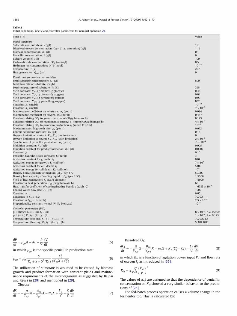
Table 2Initial conditions, kinetic and controller parameters for nominal operation 29.

Time t ðhÞ Value

Initial conditionsSubstrate concentration: S (g/l) 15Dissolved oxygen concentration: CLð¼ C�L at saturation) (g/l) 1.16Biomass concentration: X (g/l) 0.1Penicillin concentration: P (g/l) 0Culture volume: V (l) 100Carbon dioxide concentration: CO2 (mmol/l) 0.5Hydrogen ion concentration: ½Hþ� (mol/l) 10�5:1

Temperature: T (k) 297Heat generation: Qrxn (cal) 0

Kinetic and parameters and variablesFeed substrate concentration: st (g/l) 600Feed flow rate of substrate: F (l/h)Feed temperature of substrate: Tf (K) 298Yield constant: Yx=s (g biomass/g glucose) 0.45Yield constant: Yx=o (g biomass/g oxygen) 0.04Yield constant: Yp=s (g penicillin/g glucose) 0.90Yield constant: Yp=o (g penicillin/g oxygen) 0.20Constant: K1 (mol/l) 10�10

Constant: K2 (mol/l) 7� 10�5

Maintenance coefficient on substrate: mx (per h) 0.014Maintenance coefficient on oxygen: mo (per h) 0.467Constant relating CO2 to growth: a1 (mmol CO2/g biomass h) 0.143Constant relating CO2 to maintenance energy: a2 (mmol CO2/g biomass h) 4� 10�7

Constant relating CO2 to penicillin production a3 (mmol CO2/l h) 10�4

Maximum specific growth rate: lx (per h) 0.092Contois saturation constant: Kx (g/l) 0.15Oxygen limitation constant: Kox ;Kop (no limitation) 0Oxygen limitation constant: Kox ;Kop (with limitation) 2� 10�2

Specific rate of penicillin production: lp (per h) :5� 10�4

Inhibition constant: Kp (g/l) 0.005Inhibition constant for product formation: KI (g/l) 0.0002Constant: p 0.10Penicillin hydrolysis rate constant: K (per h) 3Arrhenius constant for growth: kg 0.04Activation energy for growth: Eg (cal/mol) 7� 103

Arrhenius constant for cell death: kd 5100Activation energy for cell death: Ed (cal/mol) 1033

Density x heat capacity of medium: qCp (per 1 �C) 50,000Density heat capacity of cooling liquid: rcCpc (per 1 �C) 1/1500Yield of heat generation: rq (cal/g biomass) 1/2000Constant in heat generation: rq2 (cal/g biomass h) 60Heat transfer coefficient of cooling/heating liquid: a (cal/h �C) 1:6783� 10�4

Cooling water flow rate: Fc (l/h) 1000Constant: b 0.60Constants in Kla : a;b 70, 0.4Constant in Floss : k (per h) 2:5� 10�4

Proportionality constant: c (mol ½Hþ�/g biomass) 10�5

Controller parameters (PID)pH: (base) Kc ; tI : ðhÞ; td : ðhÞ 8� 10�4, 4.2, 0.2625pH: (acid) Kc ; tI : ðhÞ; td : ðhÞ 1� 10�4, 8.4, 0.125Temperature: (cooling) Kc ; tI : ðhÞ; td : ðhÞ 70, 0.5, 1.6Temperature: (heating) Kc ; tI : ðhÞ; td : ðhÞ 5, 0.8, 0.05

1164 A. Ashoori et al. / Journal of Process Control 19 (2009) 1162–1173

dPdt¼ lppX � KP � P

VdVdt

ð5Þ

in which lpp is the specific penicillin production rate:

lpp ¼ lpS

ðKp þ Sþ S2=K1ÞCp

L

ðKopX þ CpLÞ

ð6Þ

The utilization of substrate is assumed to be caused by biomassgrowth and product formation with constant yields and mainte-nance requirements of the microorganism as suggested by Bajpaiand Reuss in [28] and mentioned in [29].

Glucose:

dSdt¼ � l

Yx=sX �

lpp

Yp=sX �mxX þ

Fsf

V� S

VdVdt

ð7Þ

Dissolved O2:

dCL

dt¼ � l

Yx=oX �

lpp

Yp=oX �moX þ KlaðC�L � CLÞ �

CL

VdVdt

ð8Þ

in which Kla is a function of agitation power input Pw and flow rateof oxygen fg as introduced in [35].

Kla ¼ affiffiffiffifg

q Pw

V

� �b

ð9Þ

The values of a;b are assigned so that the dependence of penicillinconcentration on Kla showed a very similar behavior to the predic-tions of [28].

The fed-batch process operation causes a volume change in thefermentor too. This is calculated by:

A. Ashoori et al. / Journal of Process Control 19 (2009) 1162–1173 1165

dVdt¼ F þ Fa=b � Floss ð10Þ

in which to consider the effect of acid/base addition on the total vol-ume change of the culture broth, the second term, Fa=b has been in-cluded [29]. Moreover, Floss has been taken to be a function oftemperature and culture volume V of the fermentation broth [29]:

Floss ¼ Vk e5ððT�ToÞ=Tv�ToÞ � 1� �

ð11Þ

where To and Tv are the freezing and boiling temperatures of theculture medium that were assumed to have the same propertiesas water, respectively.

The volumetric heat production rate is given as:

dQrxn

dt¼ rq1

dXdt

V þ rq2XV ð12Þ

where rq1 is assumed to be constant and might be treated as a yieldcoefficient [36].

During the product synthesis phase, when the rate of biomassformation becomes very small there is still significant heat gener-ation from metabolic maintenance activities. Hence, the secondterm in Eq. (12) is included to account for the heat production dur-ing maintenance.

Because the heat generation and CO2 evolution show similarprofiles, their production rate due to growth (dX/dt) and biomass(X) should have the same ratio as a first approximation. Based onthis observation, rq2 is calculated and tabulated in Table 2 [29].

The energy balance is written based on a coiled type heat ex-changer which is suitable for a laboratory scale fermentor [37]:

dTdt¼ F

sfðTf � TÞ þ 1

VqCp� Qrxn �

aFbþ1c

Fc þ ðaFbc=2qccpc

" #ð13Þ

The variable CO2, from which biomass may be predicted withhigh accuracy. CO2 evolution is assumed to be due to growth, pen-icillin biosynthesis and maintenance requirements [29] as sug-gested by [38]. The CO2 evolution is:

dCO2

dt¼ a1

dXdtþ a2X þ a3 ð14Þ

Here, the values of a1;a2;a3 are chosen to give CO2 profiles sim-ilar to the predictions of [38]. CO2 evolution is nearly the same asoxygen demand for penicillin production using glucose as a sub-strate and CO2 evolution trend levels off after the fed-batch switchas expected.

The extended model developed in [29] and mentioned herebriefly consists of some differential equations that are solvedsimultaneously.

3. Predictive controller design

Predictive control has been accepted as a useful advancedindustrial control technique in recent years [39]. It took more than15 years after MPC appeared in industry as an effective means tocope with constraints on the state or the control signal controlproblems, its mathematical background appeared in a steadyframework. The issues of feasibility of the online optimization, sta-bility and performance are acceptably understood for systems de-scribed by linear models. Many challenges have been made onthese issues for nonlinear systems too, but there are many ques-tions remaining about the practical applications.

MPC is mostly formulated in the state space. The nonlinear sys-tem to be controlled is described by a discrete time model [9].

xðkþ 1Þ ¼ f ðxðkÞ;uðkÞ;dðkÞÞ; xð0Þ ¼ x0 ð15Þ

where xðkÞ;uðkÞ, and dðkÞ denote the state, control, and disturbancerespectively. A receding horizon implementation is typically formu-lated by introducing the following optimization problem.

minXNp

i¼1

xTðiÞQxðiÞ þXNc

i¼1

uTðiÞRuðiÞ s:t: Exþ Fu 6 W ð16Þ

where Np is the prediction horizon, Nc is the control horizon, andE; F;W are matrices with appropriate dimensions to x and u, whichdescribe the constraints. MPC is performed by determining the con-trol signal using this cost function minimization in each step. But,only the first element of the calculated sequence is applied to theplant and this process is to be continued in next steps for shiftedhorizons. This optimization problem solves for a sequence of futureinput changes designed to minimize the objective over a predictionhorizon of length Np [10]. In this setup, yet no disturbance dðkÞ issupposed to occur.

The weighting matrices, Q, and R are used to trade off setpointtracking and manipulated variable movement, respectively. More-over, there are physical constraints on acid and base flow rates andthey could not exceed 0.1 ml/h [29] to keep the cells from starvingand to avoid all of them being washed out of the bioreactor, butany realistic cool water flow rate is available.

To avoid high computational cost dealing with nonlinear opti-mization, a linearized model of penicillin fermentation processhas been chosen near its working point [40]. In fact, the originalmodel parameters are varying with respect to time but most ofthem have a small variation range during the entire simulationtime. For the variables with wide ranges of variation, such as bio-mass concentration, the mean of their maximum and minimum va-lue was taken into account as empirically achieved to lead to betterperformance. Actually, this model would not lead to acceptableperformance if process variables vary far from its working point,since some information of the process original model has not beenconsidered. This model consists of six transfer functions [40], sinceit has three inputs (cool water, acid and base flow rates) and twooutputs (temperature and pH). Here the problem mainly is con-cerned with the transfer function from cool water flow rate totemperature:

G23 ¼BðzÞAðzÞ ¼

:9234�4000:1126e5 zþ :9234

:1126e5

z2 þ :6686e4:1126e5 z� 1:168

:1126e5

ð17Þ

which is an unstable transfer function. The predictors to predict Np

further control signals are described as in a generalized predictivecontroller framework (for linear systems) [41]:

uðtÞ ¼ Ruðt � 1Þ þ SyðtÞ þ KucðtÞ ð18Þ

in which ucðtÞ is the setpoint; 298 K, uðt � 1Þ is the previous controlinput, yðtÞ is the current output and R; S are calculated using themethod introduced in [39] and used in [40].

It should be noted that due to the highly nonlinear and open-loop unstable nature of this bioprocess, the MPC formulation isnot able to deal efficiently with setpoint tracking. This is mainlydue to failures in the ODE solver and hence to reach better perfor-mance, the regulation of the temperature to 298 K has coarselybeen chosen as a cost function regarding movements of control sig-nal [40]. This method led to a closed form controller, which ismuch easier than empirically tuning an auto-tuned PID. It isnoticeable that the constraints are applied in a suboptimal fashion,whereby candidate solutions exceeding these bounds are insteadreplaced by the bounds themselves.

The algorithm was implemented in MATLAB and the optimiza-tion was solved on-line, at each time step. The sampling time was0.05 h, which is acceptable for practical use. Prediction and controlhorizon both selected as 24 h and the weighting factors used wereQ = 1, and R ¼ 0:2 ðk ¼ 0:2Þ as mentioned before. Initial conditions

0 50 100 150 200 250 300 350 400296

297

298

299

300

301

302

Time, h

Tem

pera

ture

, K

Fig. 2. Temperature with initial substrate and biomass concentrations of 15 g/l and0.1 g/l, respectively.

0 50 100 150 200 250 300 350 4000

2

4

6

8

10

12

14

16

18

20

Time, h

Wat

er F

low

Rat

e, m

l/h

Fig. 3. Cool water flow rate.

0 50 100 150 200 250 300 350 4004.91

4.92

4.93

4.94

4.95

4.96

4.97

4.98

4.99

5

5.01

Time, h

pH

Fig. 4. pH.

Fig. 5. Penicillin concentration.

1166 A. Ashoori et al. / Journal of Process Control 19 (2009) 1162–1173

are chosen the same as the ones in [29]. The temperature and thecontrol signal, which is cool water flow rate, are shown in Figs. 2and 3 respectively.

Fig. 6. Acid and b

The pH and penicillin concentration are also provided in Figs. 4and 5 respectively. In this setup, yet pH is to be controlled througha PID controller. As can be seen in the figures, the fluctuations of

ase flow rate.

0 50 100 150 200 250 300 350 4000

0.005

0.01

0.015

0.02

0.025

0.03

0.035

0.04

0.045

0.05

Time (h)

Subs

trate

feed

Rat

e, L

/h

Fig. 7. Substrate feed rate.

A. Ashoori et al. / Journal of Process Control 19 (2009) 1162–1173 1167

the control signals are much less than the ones provided in [29].The penicillin concentration, which is the final goal, is almostgreater than the one mentioned in [29] too, but yet below 1.4 g/l.These are due to using predictive control. Since conventional con-trollers just make ad-hoc decisions regarding the current error sig-nal, but the predictive controller considers future error signals aswell to make a convenient decision. It is noticeable that althoughtemperature has more fluctuations around 298 K, but pH is almostset to 5 without directly being controlled by predictive approach,which is due to their close relationship in the model. The acid,and base flow rates are provided in Fig. 6, and the substrate feedrate is also depicted in Fig. 7. The other parameters can be observedin Fig. 8.

In this part, taking into account the high computational cost ofnonlinear optimization, the predictive approach was proposed tocontrol the linearized process. This led to a higher product concen-tration than the one provided in [29] with less fluctuations of thecontrol signal, which is the cool water flow rate. The merit of this

0 100 200 300 4000

10

20

Time, hSubs

trate

con

c. ,

g/L

0 100 200 300 4000

10

20

Time, hBiom

ass

conc

. , g

/L

0 100 200 300 40095

100

105

Time, h

Cul

ture

vol

. , L

Fig. 8. Other proc

method is its low computational cost of solving the optimizationproblem, while leading to a closed form controller, that is mucheasier than empirically tuning an auto-tuned PID. But, yet betterperformance could be performed by nonlinear optimization, whichis to be discussed in the next section.

4. Nonlinear predictive approach

As mentioned before, due to the highly nonlinear and open-loopunstable nature of this bioprocess, the MPC formulation is not ableto deal efficiently with setpoint tracking. This is mainly due to fail-ures in the ODE solver and to the severe ill-conditioning of theoptimization problem. To overcome these difficulties and toachieve better performance, the inverse of penicillin concentrationhas been chosen as a cost function regarding movements of manip-ulated variables in this section. In addition, the weighting coeffi-cients are chosen such that these two terms have the same orderof the magnitude too. Hence, the optimization problem is trans-formed into the following form:

min 0:001 �XNp

i¼1

1=PðiÞ þ 10 �XNc

i¼1

DuTðiÞDuðiÞ s:t: ua;ub 6 0:1

ð19Þ

where the input vector consists of cool water flow rate, acid andbase flow rate.

It is noticeable that in this part as well as in Section 3 the opti-mization problem can be solved for manipulating substrate feedrate as studied in [9,25,42,43] too. However, it is a bit easier to con-trol bioreactors concerning variables, such as pH and temperature,for optimizing the microbial growth [3]. Since these are the idealvariables and often have negligible perturbations. Variables subjectto large fluctuations, such as substrate can be a bit difficult to dealwith. For instance, too much substrate can be toxic while too littlecan force an early stationary phase or the onset of endogenous de-cay (i.e., death by starvation) [9].

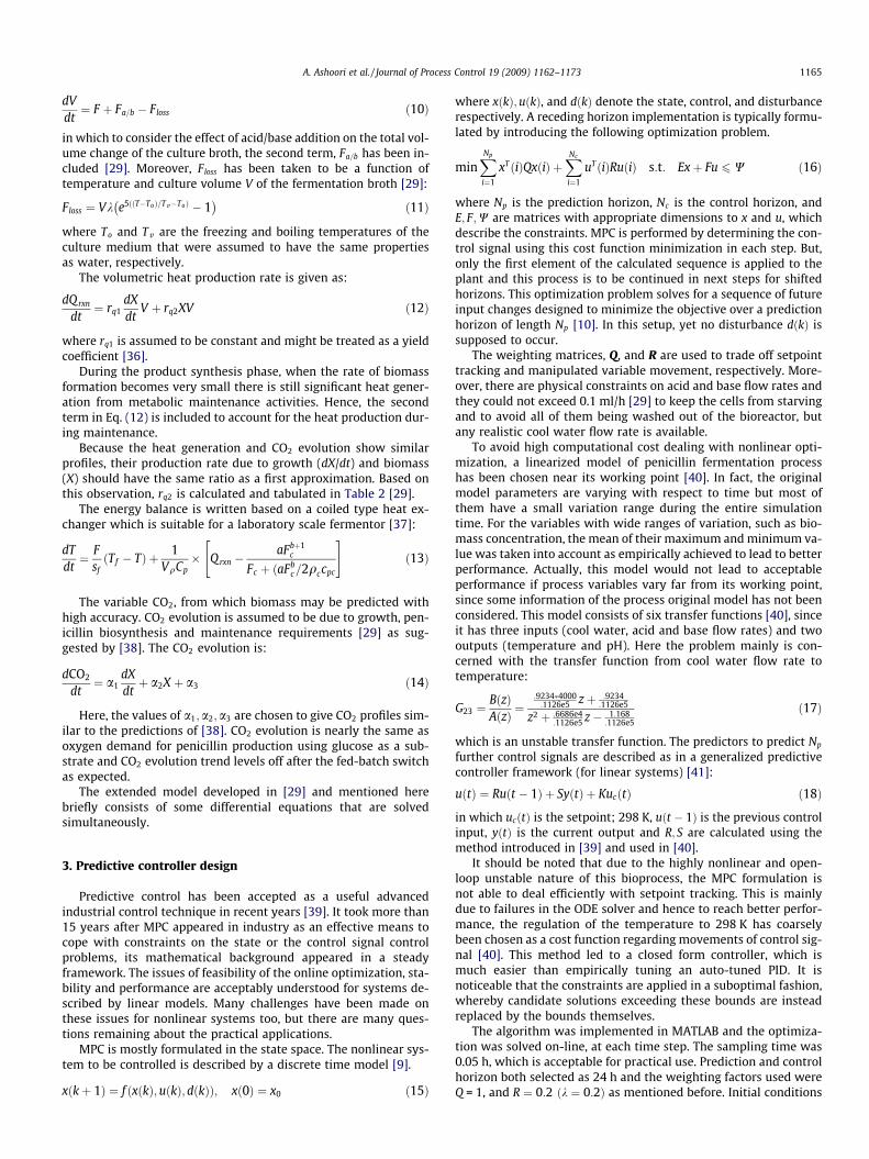
As shown in Fig. 9, MPC is performed by determining the con-trol signal by minimizing this cost function in each step regardingthe nonlinear original model used for prediction [44,10]. The solu-

0 100 200 300 40090

95

100

Time, h

DO

, %sa

tura

tion

0 100 200 300 4000

5

10x 104

Time, hGen

erat

ed h

eat ,

kca

l/L

0 100 200 300 4000

2

4

Time, h

CO

2 co

nc. ,

mm

ole/

L

ess variables.

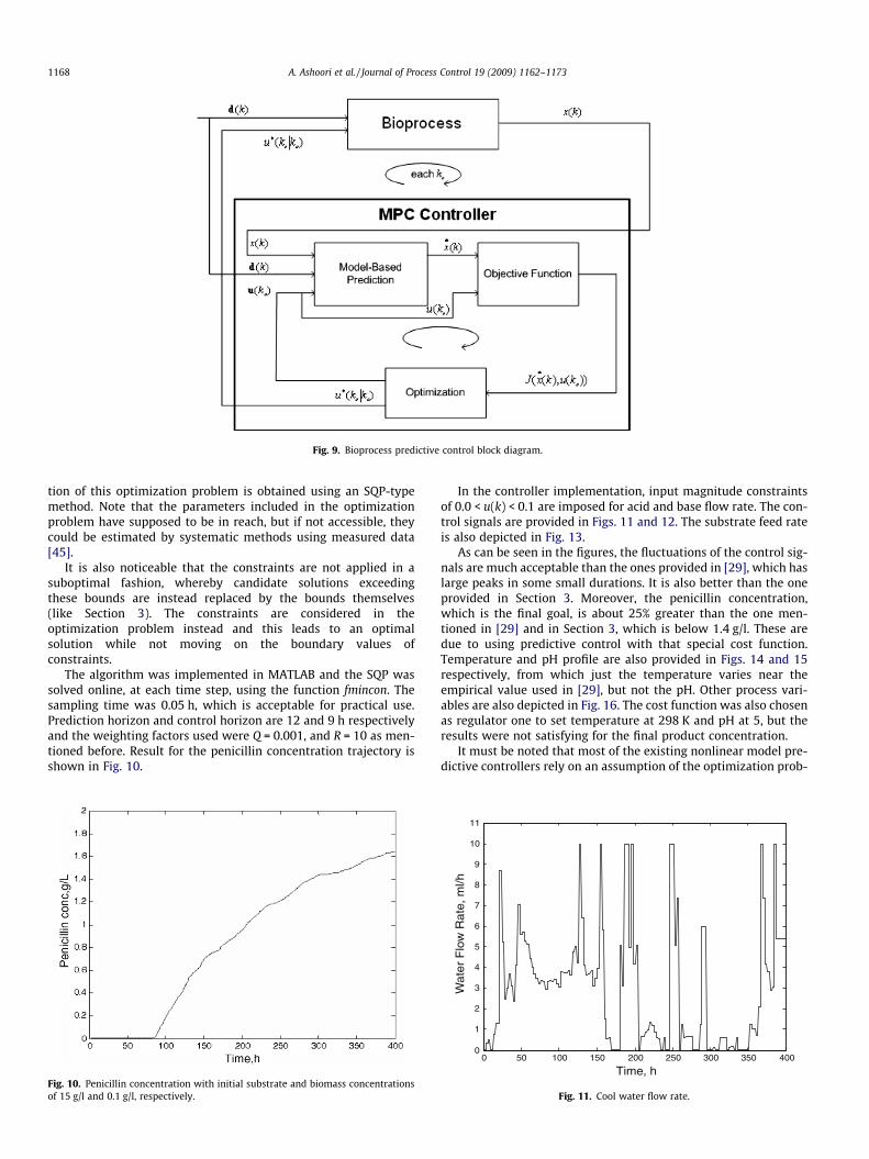
Fig. 9. Bioprocess predictive control block diagram.

1168 A. Ashoori et al. / Journal of Process Control 19 (2009) 1162–1173

tion of this optimization problem is obtained using an SQP-typemethod. Note that the parameters included in the optimizationproblem have supposed to be in reach, but if not accessible, theycould be estimated by systematic methods using measured data[45].

It is also noticeable that the constraints are not applied in asuboptimal fashion, whereby candidate solutions exceedingthese bounds are instead replaced by the bounds themselves(like Section 3). The constraints are considered in theoptimization problem instead and this leads to an optimalsolution while not moving on the boundary values ofconstraints.

The algorithm was implemented in MATLAB and the SQP wassolved online, at each time step, using the function fmincon. Thesampling time was 0.05 h, which is acceptable for practical use.Prediction horizon and control horizon are 12 and 9 h respectivelyand the weighting factors used were Q = 0.001, and R = 10 as men-tioned before. Result for the penicillin concentration trajectory isshown in Fig. 10.

Fig. 10. Penicillin concentration with initial substrate and biomass concentrationsof 15 g/l and 0.1 g/l, respectively.

In the controller implementation, input magnitude constraintsof 0.0 < u(k) < 0.1 are imposed for acid and base flow rate. The con-trol signals are provided in Figs. 11 and 12. The substrate feed rateis also depicted in Fig. 13.

As can be seen in the figures, the fluctuations of the control sig-nals are much acceptable than the ones provided in [29], which haslarge peaks in some small durations. It is also better than the oneprovided in Section 3. Moreover, the penicillin concentration,which is the final goal, is about 25% greater than the one men-tioned in [29] and in Section 3, which is below 1.4 g/l. These aredue to using predictive control with that special cost function.Temperature and pH profile are also provided in Figs. 14 and 15respectively, from which just the temperature varies near theempirical value used in [29], but not the pH. Other process vari-ables are also depicted in Fig. 16. The cost function was also chosenas regulator one to set temperature at 298 K and pH at 5, but theresults were not satisfying for the final product concentration.

It must be noted that most of the existing nonlinear model pre-dictive controllers rely on an assumption of the optimization prob-

0 50 100 150 200 250 300 350 4000

1

2

3

4

5

6

7

8

9

10

11

Time, h

Wa

ter

Flo

w R

ate

, m

l/h

Fig. 11. Cool water flow rate.

Fig. 12. Acid and base flow rate.

0 50 100 150 200 250 300 350 4000

0.005

0.01

0.015

0.02

0.025

0.03

0.035

0.04

0.045

0.05

Time (h)

Subs

trate

feed

Rat

e, L

/h

Fig. 13. Substrate feed rate.

0 50 100 150 200 250 300 350 400297.5

298

298.5

299

299.5

300

300.5

301

Time, h

Tem

pera

ture

, K

Fig. 14. Temperature.

0 50 100 150 200 250 300 350 4005

5.5

6

6.5

7

7.5

8

8.5

9

Time, h

pH

Fig. 15. pH.

A. Ashoori et al. / Journal of Process Control 19 (2009) 1162–1173 1169

lem to achieve stabilization. Some recent results on Lyapunov-based model predictive control of nonlinear systems, where appro-priate constraints are included in the optimization problem so that

the optimization problem is guaranteed to be feasible have alsobeen achieved. They are based on beginning from a characterizedset of conditions, mimicking the stability region obtained byLyapunov-based bounded controllers, handling input [46] andstate constraints [47] as well as uncertainty [48] without resortingto a min–max formulation. The set of mentioned initial conditionscould be enhanced as most recently introduced in [49] as well. Thispaper relies on the aforementioned assumption of achieve stabil-ization beginning from the same initial condition mentioned in[29]. It can easily be deducted from the figures that the stabilityhas been reached and hence a Lyapunov function exists for thisnonlinear predictive framework, which analytically is not easy tofind.

5. LoLiMoT based predictive controller

This model defined in Section 2 is definitely nonlinear andhence the optimization problem for predictive controller, whichwas fully discussed in Section 4, will lead to high computationalcost. To overcome this problem, piecewise linear models are uti-lized to simplify that nonlinear model and finally lessen computa-tional cost. The models are selected using offline identificationfrom the associated data. Moreover, the fuzzy weights of thesemodels are chosen by a neural network, such that the differencebetween local models output and the nonlinear model output

Fig. 17. Multiple-model (including locally linear neuro-fuzzy models) structure.

0 100 200 300 4000

10

20

Time, hSubs

trate

con

c. ,

g/L

0 100 200 300 4000.5

1

1.5

Time, h

DO

, % s

atur

atio

n

0 100 200 300 4000

10

20

Time, h

Biom

ass

cnc.

, g/

L

0 100 200 300 4000

5

10x 104

Time, hGen

erat

ed h

eat,

kcal

/L0 100 200 300 400

100

150

200

Time, h

Cul

ture

vol

. , L

0 100 200 300 4000

1

2

3

Time, hC

O2

Con

c. ,

mm

ole/

L

Fig. 16. Other process variables.

1170 A. Ashoori et al. / Journal of Process Control 19 (2009) 1162–1173

become as least as possible (Fig. 17). This neural network is trainedand used just to build up locally linear neuro-fuzzy (LLNF) modelsfor simplifying the original nonlinear model and the control designremains in predictive framework.

The fundamental approach with the LLNF model is to divide theinput space into small linear subspaces with fuzzy validity func-tions, which describe the validity of each linear model in its regionas a fuzzy neuron [50]. Thus, the total model is a neuro-fuzzy net-work with one hidden layer, and a linear neuron in the outputlayer, which simply calculates the weighted sum of the outputsof locally linear models (LLMs). These LLMs have basically the sameinterpretation as Takagi–Sugeno models [23] (with some assump-tion on parameters), but parameter estimation in TS models is a lit-tle bit difficult and hence, that big model is just broken into severalsmaller LLNF models and LoLiMoT estimates the parameters forthese ‘‘small” models, which is easier:

yi ¼ xi0 þxilul þxi2u2 þ � � � þxipup ð20Þ

y ¼XM

i¼1

yi/iðuÞ ð21Þ

where u ¼ ½u1u2 � � � up�T is the model input, M is the number of LLMneurons, and xij denotes the linear estimation parameters of the ithneuron. The validity functions are chosen as normalized Gaussians:

/iðuÞ ¼liðuÞPMj¼1ljðuÞ

ð22Þ

liðuÞ ¼ exp �12ðu1 � cilÞ2

r2il

þ � � � þ ðup � cipÞ2

r2ip

! !

¼ exp �12ðu1 � cilÞ2

r2il

!� � � � � exp �1

2ðup � cipÞ2

r2ip

!ð23Þ

Fig. 18. Topology of locally linear neuro-fuzzy model.

Fig. 19. Five iterations of LoLiMoT algorithm for two-dimensional input space.

A. Ashoori et al. / Journal of Process Control 19 (2009) 1162–1173 1171

The topology of network is provided in Fig. 18.The 2M � p parameters of the nonlinear hidden layer are the

parameters of Gaussian validity functions: center ðcijÞ and standarddeviation ðrijÞ. Optimization or learning methods are used to ad-just the two sets of parameters, the rule consequent parametersof the locally linear models (xij’s) and the rule premise parametersof validity functions (cij’s and rij’s). Global optimization of linearconsequent parameters is simply obtained by the Least-Squarestechnique [51,52]. The complete parameter vector containsM � ðpþ 1Þ elements:

x ¼ ½x10 x11 � � � x1p x20 x21 � � � xM0 � � � xMp�ð24Þ

and the associated regression matrix X for N measured data samplesis:

X ¼ ½X1 X2 � � � XM� ð25Þ

where:

Xi ¼

/iðuð1ÞÞ u1ð1Þ/iðuð1ÞÞ � � � upð1Þ/iðuð1ÞÞ/iðuð2ÞÞ u1ð2Þ/iðuð2ÞÞ � � � upð2Þ/iðuð2ÞÞ

..

. ... ..

.

/iðuðNÞÞ u1ðNÞ/iðuðNÞÞ � � � upðNÞ/iðuðNÞÞ

266664

377775 ð26Þ

thus:

y ¼ Xx ð27Þ

x ¼ XT X þ aI� ��1

XT y; a 6 1 ð28Þ

a is the regularization parameter for avoiding any near singularityof matrix XT X in Eq. (28). The remarkable properties of locally linearneuro-fuzzy model, its transparency and intuitive construction, leadto the use of least squares technique [51,52] for rule antecedentparameters.

An incremental tree-based learning algorithm, e.g. locally linearmodel tree (LoLiMoT) [50], is appropriate for tuning the rule pre-mise parameters, i.e. determining the validation hypercube foreach locally linear model. In each iteration, the worst performinglocally linear neuron is determined to be divided. All the possibledivisions in the p-dimensional input space are checked and thebest is performed. The splitting ratio can be simply adjusted as0.5; which means that the locally linear neuron is divided intotwo equal halves. The fuzzy validity functions for the new struc-

ture are updated; their centers are the centers of the new hyper-cubes, and the standard deviations are usually set as 0.7. Thealgorithm is as follows:

(1) The initial model: Start with a single locally linear neuron,which is a globally optimal linear least- squares estimationover the whole input space with /1ðuÞ ¼ 1 and M ¼ 1.

(2) Find the worst neuron: Calculate a local loss function, e.g.MSE for each of the i ¼ 1; . . . ;M locally linear neurons, andfind the worst performing neuron.

(3) Check all divisions: The worst neuron is considered for fur-ther refinement. The validation hypercube of this neuron isdivided into two halves with an axis orthogonal split. Divi-sions in all dimensions are tried, and for each of the p divi-sions the following steps are carried out:

(a) Construction of the multi-dimensional validity func-

tions for both generated hypercubes.(b) Local estimation of the rule consequent parameters

for both newly generated neurons.(c) Calculation of the total loss function or error index for

the current overall model.

4) Validate the best division: The best of the p alternatives inStep 3 is selected. If it results in reduction of loss functionsor error indices on training and validation data sets, therelated validity functions and neurons are updated, thenumber of neurons is incremented M ¼ M þ 1; and the algo-rithm continues from Step 2, otherwise the learning algo-rithm is terminated.

0 5 10 15 20 25 3010-20

10-19

10-18

10-17

10-16

10-15

10-14

10-13

Neurons No.

Sol

id :

Trai

n M

SE

, D

otte

d : T

est M

SE

Fig. 20. Training and test error versus the number of the neurons in the middlelayer of the neural network used to estimate penicillin concentration.

1172 A. Ashoori et al. / Journal of Process Control 19 (2009) 1162–1173

In Fig. 19, the algorithm is represented for two-dimensional in-put spaces. This automatic learning algorithm provides the bestlinear or nonlinear model with maximum generalization, and per-forms well in prediction applications [53].

As mentioned in the beginning of this section, this algorithmwas applied to the nonlinear model output data for each output(so nine networks were trained) in order to get a bank of locallylinear models to reduce the optimization computation time forpredicting future outputs using this network instead of the originalmodel [53]. If for some outputs the test data error did not form aconvex form, in which the minimum is the optimal number ofthe neurons [50], then it can be deducted that a linear model usinga simple method such as LS had sufficed for that output (e.g. Fig. 20for penicillin concentration output). The final product concentra-tion was as same as the one shown in Fig. 10 and had not changedeffectively, but the computational cost as expected reduced almostto one fourth.

6. Conclusion

In this article, taking into account the nonlinearity of thepenicillin fermentation process, the predictive approach wasproposed to control that. The linear version was applied ini-tially, but acceptable performance was not achieved, hence,the optimization problem was solved to reach the maximumconcentration for final product, which is the penicillin whileneglecting the empirical setpoints for the temperature and pH.Meanwhile, fluctuations of control signals, which are acid, baseand cool water flow rates were also taken into account in orderto getting prepared for its practical implementation. This led toa better product than the one provided in [29] with moreacceptable fluctuations of control signals. The merit of thismethod is that it directly solves the optimization problem toobtain maximum possible product concentration, while notviolating physical constraints for acid and base flow rates.Moreover, utilizing LoLiMoT based model, the computationalcost is also very acceptable for a real time process.

Acknowledgements

The authors want to thank the team working on PENSIM in Illi-nois Institute of Technology for providing the data for this project.

The authors also want to especially thank Dr. Cinar because of hiskind guidance.

References

[1] J. Liang, Y.Q. Chen, Optimization of a fed-batch fermentation process controlcompetition problem using the NEOS server, Proceedings of the I MECH E Part IJournal of Systems and Control Engineering I5 (2003) 427–432.

[2] A. Johnson, The control of fed-batch fermentation processes: a survey,Automatica 23 (6) (1987) 691–705.

[3] R. Aguilar, J. Gonzalz, M.A. Barron, R. Martinez-Guerra, R. Maya-Yescas, RobustPI2 controller for continuous bioreactors, Process Biochemistry 36 (2000)1007–1013.

[4] J.S. Alford, Bioprocess control: advances and challenges, Journal of Computersand Chemical Engineering 30 (2006) 1464–1475.

[5] F. Renard, A.V. Wouwer, Robust adaptive control of yeast fed-batch cultures,Journal of Computers and Chemical Engineering 32 (2008) 1238–1248.

[6] S. Sugimoto, M. Yabuta, N. Kato, T. Seki, T. Yoshida, H. Taguchi,Hyperproduction of phenylalanine by Escherichia coli, Journal ofBiotechnology 5 (1987) 237–253.

[7] K.B. Konstantinov, T. Yoshida, A knowledge-based pattern recognitionapproach for real-time diagnosis and control of fermentation processes asvariable structure plants, IEEE Transactions on Systems, Man, and Cybernetics21 (4) (1991) 908–914.

[8] J. Horiuchi, Fuzzy modeling and control of biological processes, Journal ofBioscience and Bioengineering 94 (6) (2002) 574–578.

[9] S. Ramaswamy, T.J. Cutright, H.K. Qammar, Control of a continuous bioreactorusing model predictive control, Journal of Process Biochemistry 40 (2005)2763–2770.

[10] R.S. Parker, Nonlinear model predictive control of a continuous bioreactorusing approximate data-driven models, in: Proceedings of the AmericanControl Conference, Anchorage, AK, USA, 2002.

[11] A.S. Soni, R.S. Parker, Fed-batch bioreactor control using a multi-scale model,in: Proceedings of the American Control Conference, Denver, Colorado, USA,2003.

[12] B. Dahhou, G. Roux, G. Chamilothoris, Modelling and adaptive predictivecontrol of a continuous fermentation process, Journal of Applied Math andModelling 16 (1992) 545–552.

[13] R. Schneider, N.A. Jalel, A. Munack, J.R. Leigh, Adaptive predictive control forthe fed-batch fermentation process, Proceedings of the Conference on ControlEngineering 389 (1994) 249–254.

[14] J.A.D. Rodrigues, R.M. Filho, Production optimization with operatingconstraints for a fed-batch reactor with DMC predictive control, Journal ofChemical Engineering Science 54 (1999) 2745–2751.

[15] K. Shimizu, An overview on the control system design of bioreactors, Advancesin Biochemical Engineering and Biotechnology 50 (1993) 65–84.

[16] K.J. Astrom, Theory and applications of adaptive control: a survey, Automatica19 (5) (1983) 471–486.

[17] H. Honda, T. Kobayashi, Fuzzy control of bioprocess, Journal of Bioscience andBioengineering 89 (5) (2000) 401–408.

[18] M. Hosobuchi, F. Fukui, H. Matsukawa, T. Suzuki, H. Yoshikawa, Fuzzy controlduring microbial production of ML-236B, a precursor of pravastatin sodium,Journal of Fermentation Technology 76 (1993) 482–486.

[19] K.B. Konstantinov, T. Yoshida, An expert approach for control of fermentationprocesses as variable structure plants, Journal of Fermentation andBioengineering 70 (1990) 48–57.

[20] K. Oishi, M. Tominaga, A. Kawato, S. Imayasu, S. Nanba, Application of fuzzycontrol theory to the sake brewing process, Journal of Fermentation andBioengineering 72 (1997) 115–121.

[21] H. Honda, T. Hanai, A. Katayama, H. Tohyama, T. Kobayashi, Temperaturecontrol of Ginjo sake mashing process by automatic fuzzy modeling usingfuzzy neural networks, Journal of Fermentation and Bioengineering 85 (1998)107–112.

[22] C. Karakuzu, M. Turker, S. Ozturk, Modelling, on-line state estimation andfuzzy control of production scale fed-batch baker’s yeast fermentation, ControlEngineering Practice 14 (2006) 959–974.

[23] T. Takagi, M. Sugeno, Fuzzy identification of systems and its application tomodeling and control, IEEE Transactions on Systems, Man, and Cybernetics 15(1) (1985) 116–132.

[24] Z. Shi, K. Shimizu, Neuro-fuzzy control of bioreactor systems with patternrecognition, Journal of Fermentation and Bioengineering 74 (1) (1992)39–45.

[25] Hisbullah, M.A. Hussain, K.B. Ramachandran, Design of a fuzzy logic controllerfor regulating substrate feed to fed-batch fermentation, Transactions ofIChemE 81 (C) (2003) 138–146.

[26] C. Valencia, G. Espinosa, J. Giralt, F. Giralt, Optimization of invertaseproduction in a fed-batch bioreactor using simulation based dynamicprogramming coupled with a neural classifier, Computers and ChemicalEngineering 31 (2007) 1131–1140.

[27] A. Handa-Corrigan, S. Nikolay, D. Fletcher, S. Mistry, A. Young, C. Ferguson,Monoclonal antibody production in hollow fiber bioreactors: process controland validation strategies for manufacturing industry, Enzyme and MicrobialTechnology 17 (3) (1995) 225–230.

[28] R. Bajpai, M. Reuss, A mechanistic model for penicillin Production, Journal ofChemical Technology and Biotechnology 30 (1980) 330–344.

A. Ashoori et al. / Journal of Process Control 19 (2009) 1162–1173 1173

[29] G. Birol, C. Undey, A. Cinar, A modular simulation package for feed-batchfermentation: penicillin production, Journal of Computers and ChemicalEngineering 26 (2002) 1553–1565.

[30] P.R. Patnaik, Penicillin fermentation: mechanisms and models for industrial-scale bioreactors, Critical Reviews in Microbiology 27 (1) (2001) 25–39.

[31] C. Zhao, F. Wang, N. Lu, M. Jia, Stage-based soft-transition multiple PCAmodeling and on-line monitoring strategy for batch processes, Journal ofProcess Control 17 (2008) 728–741.

[32] J. Heijnen, J. Roels, A. Stouthamer, Application of balancing methods inmodeling the penicillin fermentation, Journal of Biotechnology andBioengineering 21 (1979) 2175–2201.

[33] G. Birol, C. Undey, S.J. Parulekar, A. Cinar, A morphologically structured modelfor penicillin production, Journal of Biotechnology and Bioengineering 77 (5)(2002) 538–552.

[34] M. Schuler, F. Kargi, Bioprocess Engineering Basic Concepts, second ed.,Prentice Hall, Saddle River, NJ, 2002.

[35] J.E. Bailey, D.F. Ollis, Biochemical Engineering Fundamentals, McGraw Hill,New York, 1986.

[36] J. Nielsen, J. Villadsen, Bioreaction Engineering Principles, Plenum Press, NewYork, 1994.

[37] J. Nielsen, Physiological Engineering Aspects of Penicillin chrysogenum, WorldScientific, Singapore, 1997.

[38] G. Montague, A. Morris, A. Wright, M. Aynsley, A. Ward, Growth monitoringand control through computer-aided on-line mass balancing in fed-batchpenicillin fermentation, Canadian Journal of Chemical Engineering 64 (1986)567–580.

[39] E.F. Camacho, C. Bordons, Model Predictive Control, Springer, 1999.[40] A. Ashoori, B. Moshiri, A. Ramezani, M.R. Bakhtiari, A. Khaki-Sedigh, pH control

of a fed-batch fermentation process using model predictive control, in:Proceedings of the 14th International Congress of Cybernetics and Systems ofWOSC, 2008, pp. 730–738.

[41] D.W. Clarke, C. Mohtadi, P.S. Tuffs, Generalized predictive control. Part I: thebasic algorithm, Automatica 23 (2) (1987) 137–148.

[42] M.A. Barro, R. Aguilar, Dynamic behaviour of continuous stirred bioreactorunder control input saturation, Journal of Chemical Technology andBiotechnology 72 (1998) 15–18.

[43] R.G. Dondo, D. Marques, Optimal control of a batch bioreactor: a study on theuse of an imperfect model, Process Biochemistry 37 (2001) 379–385.

[44] E.S. Meadows, J.B. Rawlings, Model Predictive Control, Nonlinear ProcessControl, Prentice Hall, 1997. pp. 233–310, Chapter 5.

[45] P. Mhaskar, M.A. Hjortso, M.A. Henson, Cell population modeling andparameter estimation for continuous cultures of Saccharomyces cerevisiae,Biotechnology Progress 18 (2002) 1010–1026.

[46] P. Mhaskar, N.H. El-Farra, P.D. Christofides, Predictive control of switchednonlinear systems with scheduled mode transitions, IEEE Transactions onAutomatic Control 50 (11) (2002) 1670–1680.

[47] P. Mhaskar, N.H. El-Farra, P.D. Christofides, Stabilization of nonlinear systemswith state and control constraints using Lyapunov-based predictive control,Systems and Control Letters 55 (2006) 650–659.

[48] P. Mhaskar, Robust model predictive control design for fault–tolerant ofprocess systems, Industrial Engineering and Chemical Resources Journal 45(2006) 8565–8574.

[49] M. Mahmood, P. Mhaskar, Enhanced stability regions for nonlinearprocess systems using model predictive control, AIChE Journal 6 (2008)1487–1498.

[50] O. Nelles, Nonlinear System Identification, Springer-Verlag, Berlin, 2001.[51] T. Kariya, H. Kurata, Generalized Least Squares, Wiley, 2004.[52] J. Wolberg, Data Analysis Using the Method of Least Squares: Extracting the

Most Information from Experiments, Springer, 2005.[53] H. Leung, T. Lo, S. Wang, Prediction of noisy chaotic time series using an

optimal radial basis function neural network, IEEE Transactions on NeuralNetworks 12 (2001) 1163–1172.