Ac

Ja

b

a

ARRAA

KMGWMM

1

ircsacsm

fsMtiafi

UT

h0

Journal of Process Control 24 (2014) 1346–1357

Contents lists available at ScienceDirect

Journal of Process Control

j our na l ho me pa g e: www.elsev ier .com/ locate / jprocont

gap metric based weighting method for multimodel predictiveontrol of MIMO nonlinear systems

ingjing Dua,b,∗, Tor Arne Johansena

Department of Engineering Cybernetics, Norwegian University of Science and Technology, NO 7491 Trondheim, NorwaySchool of Electrical Engineering and Automation, Henan Polytechnic University, Jiaozuo 454000, China

r t i c l e i n f o

rticle history:eceived 5 November 2013eceived in revised form 27 April 2014ccepted 2 June 2014vailable online 16 July 2014

a b s t r a c t

A novel weighting method is proposed for multimodel predictive control of nonlinear systems with mul-tiple scheduling variables (MIMO nonlinear systems), in which the gap metric is employed to formulateweighting functions for local controller combination. Compared to existent weighting functions, the pro-posed weighting method has two major advantages: firstly, there is only one tuning parameter, whichmakes it simpler. Secondly, the weights depend only on the scheduling vector and can be calculated

eywords:ultimodel predictive controlap metriceighting functionIMO nonlinear systemultiple scheduling variables

off-line and stored in a look-up table. Therefore, the computational load can be reduced, especially fornonlinear systems with multiple scheduling variables. A MIMO CSTR system is studied to demonstratethe effectiveness of the proposed weighting method.

© 2014 Elsevier Ltd. All rights reserved.

. Introduction

The multimodel approach has attracted a lot of attention forts ability to deal with nonlinear systems with a wide operatingange [1–6]. The multimodel approach is based on the “divide andonquer” principle: first decompose a nonlinear system into linearubsystems, second design a controller for every linear subsystem,nd finally combine the local controllers into a global one. For localontroller combination, there are mainly two types of methods:witching (hard switching) methods and weighting (soft switching)ethods [1].In the switching methods, the key is to find a proper per-

ormance index, according to which only one local controller iselected to be used in the feedback loop at every sample period.any different performance indices have been used in the litera-

ure, e.g., index of output error [3], index of estimate error [4,7],ndex of operating conditions [2], and so on. Although it may beble to select the best possible local linear controller to put into the

eedback loop, the switching method can lead to output chatteringn systems with strong nonlinearities.

∗ Corresponding author at: Department of Engineering Cybernetics, Norwegianniversity of Science and Technology, NO 7491 Trondheim, Norway.el.: +47 94297992.

E-mail address: jjdu@hpu.edu.cn (J. Du).

ttp://dx.doi.org/10.1016/j.jprocont.2014.06.002959-1524/© 2014 Elsevier Ltd. All rights reserved.

In the weighting methods, the key is to find proper weightingfunctions. The global controller is then defined by a weighted sum oflocal controllers’ outputs or parameters. There are many weightingfunctions available, such as Gaussian functions [8–11], trapezoidalfunctions [12], Bayesian weighting functions [5,13,14], and so on.Generally speaking, the weighting method appears more promisingto combine controllers, as the weighted average of local controllersmakes the system outputs smooth and can reduce or avoid out-put chattering. However, it is not trivial to find proper weightingfunctions, because usually there is more than one parameter to bedetermined by a prior knowledge and experience, and differentchoices lead to different weights.

In recent years, the gap metric has been used a lot in the multi-model framework [6,10,12,15,16], mostly for model bank selectionand reduction. An exception was the work of Arslan et al. [17],where the gap metric was used to form weighting functions to com-bine local controllers. The weighting functions were constructed bya defined closed-loop gap metric. However, the weighting functionsin [17] were complicated to compute as closed-loop systems wereconsidered. Besides, the method could not be applied to constrainedmodel predictive control (MPC) since an explicit transfer function ofthe local controller was needed in the definition of closed-loop gapmetric. In this paper, we make full use of the advantage of the

open-loop gap metric to develop an efficient and simple methodto construct weighting functions for multimodel predictive controlof MIMO nonlinear systems, which can be used regardless of thecontrol algorithm.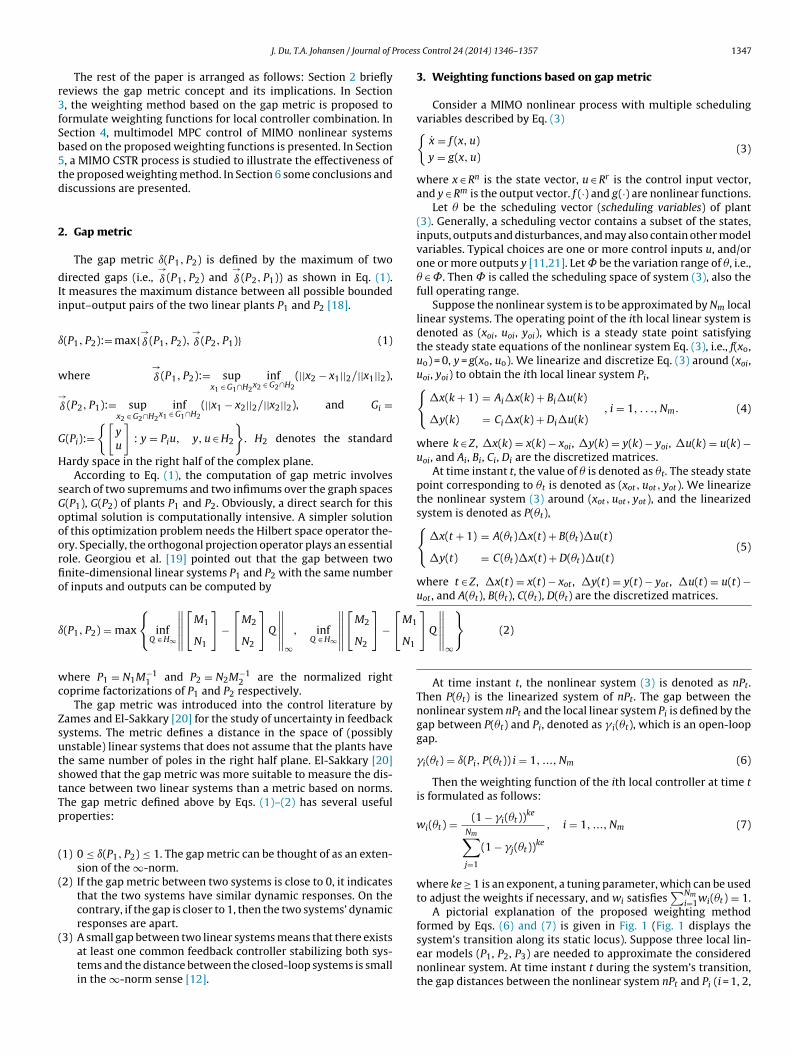

roces

r3fSb5td

2

dIi

ı

w

→

G

H

sGooorfio

ı

[M1

N1

wc

ZsutstTp

(

(

(

J. Du, T.A. Johansen / Journal of P

The rest of the paper is arranged as follows: Section 2 brieflyeviews the gap metric concept and its implications. In Section, the weighting method based on the gap metric is proposed toormulate weighting functions for local controller combination. Inection 4, multimodel MPC control of MIMO nonlinear systemsased on the proposed weighting functions is presented. In Section, a MIMO CSTR process is studied to illustrate the effectiveness ofhe proposed weighting method. In Section 6 some conclusions andiscussions are presented.

. Gap metric

The gap metric ı(P1, P2) is defined by the maximum of two

irected gaps (i.e.,→ı (P1, P2) and

→ı (P2, P1)) as shown in Eq. (1).

t measures the maximum distance between all possible boundednput–output pairs of the two linear plants P1 and P2 [18].

(P1, P2):= max{→ı (P1, P2),

→ı (P2, P1)} (1)

here→ı (P1, P2):= sup

x1 ∈ G1∩H2

infx2 ∈ G2∩H2

(||x2 − x1||2/||x1||2),

ı (P2, P1):= supx2 ∈ G2∩H2

infx1 ∈ G1∩H2

(||x1 − x2||2/||x2||2), and Gi =

(Pi):={[

yu

]: y = Piu, y, u ∈ H2

}. H2 denotes the standard

ardy space in the right half of the complex plane.According to Eq. (1), the computation of gap metric involves

earch of two supremums and two infimums over the graph spaces(P1), G(P2) of plants P1 and P2. Obviously, a direct search for thisptimal solution is computationally intensive. A simpler solutionf this optimization problem needs the Hilbert space operator the-ry. Specially, the orthogonal projection operator plays an essentialole. Georgiou et al. [19] pointed out that the gap between twonite-dimensional linear systems P1 and P2 with the same numberf inputs and outputs can be computed by

(P1, P2) = max

{inf

Q ∈ H∞

∥∥∥∥∥[

M1

N1

]−

[M2

N2

]Q

∥∥∥∥∥∞

, infQ ∈ H∞

∥∥∥∥∥[

M2

N2

]−

here P1 = N1M−11 and P2 = N2M−1

2 are the normalized rightoprime factorizations of P1 and P2 respectively.

The gap metric was introduced into the control literature byames and El-Sakkary [20] for the study of uncertainty in feedbackystems. The metric defines a distance in the space of (possiblynstable) linear systems that does not assume that the plants havehe same number of poles in the right half plane. El-Sakkary [20]howed that the gap metric was more suitable to measure the dis-ance between two linear systems than a metric based on norms.he gap metric defined above by Eqs. (1)–(2) has several usefulroperties:

1) 0 ≤ ı(P1, P2) ≤ 1. The gap metric can be thought of as an exten-sion of the ∞-norm.

2) If the gap metric between two systems is close to 0, it indicatesthat the two systems have similar dynamic responses. On thecontrary, if the gap is closer to 1, then the two systems’ dynamicresponses are apart.

3) A small gap between two linear systems means that there existsat least one common feedback controller stabilizing both sys-tems and the distance between the closed-loop systems is smallin the ∞-norm sense [12].

s Control 24 (2014) 1346–1357 1347

]Q

∥∥∥∥∥∞

}(2)

3. Weighting functions based on gap metric

Consider a MIMO nonlinear process with multiple schedulingvariables described by Eq. (3){

x = f (x, u)

y = g(x, u)(3)

where x ∈ Rn is the state vector, u ∈ Rr is the control input vector,and y ∈ Rm is the output vector. f (·) and g(·) are nonlinear functions.

Let � be the scheduling vector (scheduling variables) of plant(3). Generally, a scheduling vector contains a subset of the states,inputs, outputs and disturbances, and may also contain other modelvariables. Typical choices are one or more control inputs u, and/orone or more outputs y [11,21]. Let be the variation range of �, i.e.,� ∈ ˚. Then is called the scheduling space of system (3), also thefull operating range.

Suppose the nonlinear system is to be approximated by Nm locallinear systems. The operating point of the ith local linear system isdenoted as (xoi, uoi, yoi), which is a steady state point satisfyingthe steady state equations of the nonlinear system Eq. (3), i.e., f(xo,uo) = 0, y = g(xo, uo). We linearize and discretize Eq. (3) around (xoi,uoi, yoi) to obtain the ith local linear system Pi,{

�x(k + 1) = Ai�x(k) + Bi�u(k)

�y(k) = Ci�x(k) + Di�u(k), i = 1, . . ., Nm. (4)

where k ∈ Z , �x(k) = x(k) − xoi, �y(k) = y(k) − yoi, �u(k) = u(k) −uoi, and Ai, Bi, Ci, Di are the discretized matrices.

At time instant t, the value of � is denoted as �t. The steady statepoint corresponding to �t is denoted as (xot, uot, yot). We linearizethe nonlinear system (3) around (xot, uot, yot), and the linearizedsystem is denoted as P(�t),{

�x(t + 1) = A(�t)�x(t) + B(�t)�u(t)

�y(t) = C(�t)�x(t) + D(�t)�u(t)(5)

where t ∈ Z , �x(t) = x(t) − xot , �y(t) = y(t) − yot , �u(t) = u(t) −uot , and A(�t), B(�t), C(�t), D(�t) are the discretized matrices.

At time instant t, the nonlinear system (3) is denoted as nPt.Then P(�t) is the linearized system of nPt. The gap between thenonlinear system nPt and the local linear system Pi is defined by thegap between P(�t) and Pi, denoted as � i(�t), which is an open-loopgap.

�i(�t) = ı(Pi, P(�t)) i = 1, ..., Nm (6)

Then the weighting function of the ith local controller at time tis formulated as follows:

wi(�t) = (1 − �i(�t))ke

Nm∑j=1

(1 − �j(�t))ke

, i = 1, ..., Nm (7)

where ke ≥ 1 is an exponent, a tuning parameter, which can be usedto adjust the weights if necessary, and wi satisfies

∑Nm

i=1wi(�t) = 1.A pictorial explanation of the proposed weighting method

formed by Eqs. (6) and (7) is given in Fig. 1 (Fig. 1 displays the

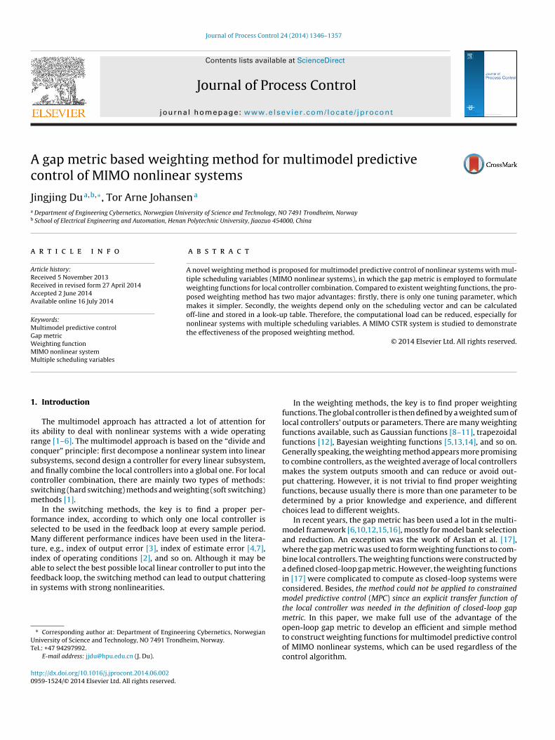
system’s transition along its static locus). Suppose three local lin-ear models (P1, P2, P3) are needed to approximate the considerednonlinear system. At time instant t during the system’s transition,the gap distances between the nonlinear system nPt and Pi (i = 1, 2,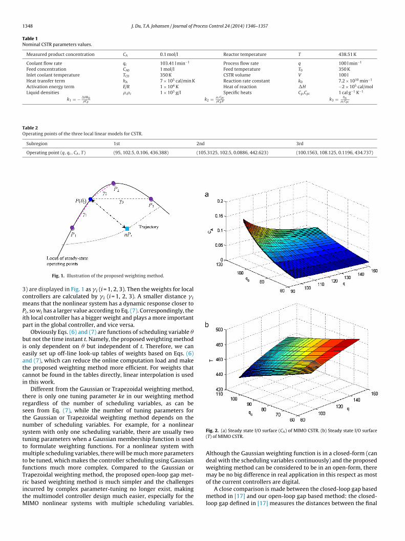

1348 J. Du, T.A. Johansen / Journal of Process Control 24 (2014) 1346–1357

Table 1Nominal CSTR parameters values.

Measured product concentration CA 0.1 mol/l Reactor temperature T 438.51 K

Coolant flow rate qc 103.41 l min−1 Process flow rate q 100 l min−1

Feed concentration CA0 1 mol/l Feed temperature T0 350 KInlet coolant temperature TC0 350 K CSTR volume V 100 lHeat transfer term hA 7 × 105 cal/min K Reaction rate constant k0 7.2 × 1010 min−1

Activation energy term E/R 1 × 104 K Heat of reaction �H −2 × 105 cal/molLiquid densities �,�c 1 × 103 g/l Specific heats Cp,Cpc 1 cal g−1 K−1

k1 = − �Hk0�Cp

k2 = �c Cpc�CpV k3 = hA

�c Cpc

Table 2Operating points of the three local linear models for CSTR.

Subregion 1st 2nd 3rd

Operating point (q, qc, CA, T) (95, 102.5, 0.106, 436.388) (105.3125, 102.5, 0.0886, 442.623) (100.1563, 108.125, 0.1196, 434.737)

3cmPip

bieatci

trstnsttmtfTritM

Fig. 1. Illustration of the proposed weighting method.

) are displayed in Fig. 1 as � i (i = 1, 2, 3). Then the weights for localontrollers are calculated by � i (i = 1, 2, 3). A smaller distance � ieans that the nonlinear system has a dynamic response closer to

i, so wi has a larger value according to Eq. (7). Correspondingly, theth local controller has a bigger weight and plays a more importantart in the global controller, and vice versa.

Obviously Eqs. (6) and (7) are functions of scheduling variable �ut not the time instant t. Namely, the proposed weighting method

s only dependent on � but independent of t. Therefore, we canasily set up off-line look-up tables of weights based on Eqs. (6)nd (7), which can reduce the online computation load and makehe proposed weighting method more efficient. For weights thatannot be found in the tables directly, linear interpolation is usedn this work.

Different from the Gaussian or Trapezoidal weighting method,here is only one tuning parameter ke in our weighting methodegardless of the number of scheduling variables, as can beeen from Eq. (7), while the number of tuning parameters forhe Gaussian or Trapezoidal weighting method depends on theumber of scheduling variables. For example, for a nonlinearystem with only one scheduling variable, there are usually twouning parameters when a Gaussian membership function is usedo formulate weighting functions. For a nonlinear system with

ultiple scheduling variables, there will be much more parameterso be tuned, which makes the controller scheduling using Gaussianunctions much more complex. Compared to the Gaussian orrapezoidal weighting method, the proposed open-loop gap met-

ic based weighting method is much simpler and the challengesncurred by complex parameter-tuning no longer exist, makinghe multimodel controller design much easier, especially for the

IMO nonlinear systems with multiple scheduling variables.

Fig. 2. (a) Steady state I/O surface (CA) of MIMO CSTR. (b) Steady state I/O surface(T) of MIMO CSTR.

Although the Gaussian weighting function is in a closed-form (candeal with the scheduling variables continuously) and the proposedweighting method can be considered to be in an open-form, theremay be no big difference in real application in this respect as most

of the current controllers are digital.

A close comparison is made between the closed-loop gap basedmethod in [17] and our open-loop gap based method: the closed-loop gap defined in [17] measures the distances between the final

J. Du, T.A. Johansen / Journal of Process Control 24 (2014) 1346–1357 1349

90100

110120

130140 150

60

80

100

1200

0.2

0.4

0.6

q

w1

90100

110120

130140 150

60

80

100

1200

0.2

0.4

0.6

qqc

w1

ke=1

ke=6

e first

diwea

c

Fig. 3. 3-D plots of th

esired closed-loop system (the final desired system has an operat-ng point equal to the setpoint) and the current closed-loop systems

ith local controllers (Ki, i = 1, 2, 3). Unfortunately, the intuitivexplanation is lost in the closed-loop gap because all the distancesre represented by the same line segment (see Fig. 1 in [17]). As

906080

100120

0

0.2

0.4

0.6

qc

w2

906080

100120

0

0.5

1

qc

w2

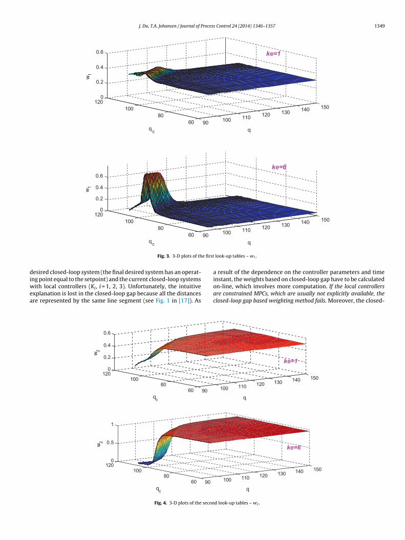
Fig. 4. 3-D plots of the secon

q

look-up tables – w1.

a result of the dependence on the controller parameters and timeinstant, the weights based on closed-loop gap have to be calculated

on-line, which involves more computation. If the local controllersare constrained MPCs, which are usually not explicitly available, theclosed-loop gap based weighting method fails. Moreover, the closed-

100 110120 130

140 150

q

100 110 120 130 140 150

q

ke=1

ke=6

d look-up tables – w2.

1350 J. Du, T.A. Johansen / Journal of Process Control 24 (2014) 1346–1357

90 100 110 120 130 140 150

6080

100120

0

0.5

1

q

w3

90 100 110 120 130 140 150

6080

100120

0

0.2

0.4

0.6

qqc

w3

ke=1

ke=6

e third

lscm

a

u

wcts

4s

mt

tdlh

d

J

A0 −

− T(

c

Fig. 5. 3-D plots of th

oop gap based method is only applicable to the cases where theetpoint is equal to one of the operating points (see the definition oflosed-loop gap in [17]). Therefore, our open-loop gap metric basedethod is more useful, intuitive and much simpler comparatively.Finally the output of the global controller is the weighted aver-

ge of the local linear controllers:

(t) =Nm∑i=1

wi(�t)ui(t) (8)

here ui is the output of the ith local linear controller. The localontrollers are scheduled according to the gap distance betweenhe nonlinear system and the local linear systems (open loop). Amaller gap distance means a larger weight, and vice versa.

. Multimodel predictive control of MIMO nonlinearystems

Model predictive control (MPC) is employed here within theultimodel framework for its advantages over traditional con-

rollers [22]: (1) MPC displays improved performance because

he process model allows current computations to consider futureynamic events. (2) MPC provides a convenient method for hand-

ing multivariable control. (3) MPC allows for the incorporation ofard and soft constraints.

Based on each local linear system Pi, a MPC controller can beesigned by considering the following cost function:

⎧⎨⎩

CA(t) = q

V[C

T(t) = q

V[T0

i =Ny∑j=1

||r(k + j) − y(k + j|k)||2Qy+

Nu∑j=1

||�ui(k + j − 1)||2Qy(9)

q

look-up tables – w3.

with constraints:⎧⎪⎨⎪⎩

umin ≤ ui ≤ umax

�ui,min ≤ �ui ≤ �ui,max

ymin ≤ y ≤ ymax

(10)

where Qy, Qu are the weighted matrix, Ny is the prediction hori-zon, Nu is the control horizon, and r is the reference signal. Eqs.(9) and (10) form a Quadratic Programming problem [23]. Inthe following simulations, we use the MPC Toolbox in Matlab tosolve it.

Therefore, Nm local MPC controllers are designed for the non-linear system (3). These local controllers are combined into oneglobal multimodel predictive controller according to Eq. (8), whereui = �ui + uoi.

5. Case study

Consider a MIMO continuous stirred tank reactor (CSTR) pro-cess, which consists of an irreversible, exothermic reaction, A → B,in a constant volume reactor cooled by a single coolant stream. Itcan be modeled by the following nonlinear equations [24]:

CA(t)] − k0CA(t)e−(E/RT(t))

t)] + k1CA(t)e−(E/RT(t)) + k2qc(t)[1 − e−(k3/qc(t))][Tc0 − T(t)](11)

The control objective is to control the measured concentration ofA, CA, and the temperature T, by manipulating the process flow rateq and coolant flow rate qc for set-point tracking control. The nom-inal parameter values are listed in Table 1. The assumed variationranges of inputs are q ∈ [95, 150] and qc ∈ [60, 110], and those ofoutputs are CA ∈ [0.02, 0.15] and T ∈ [430, 490]. As can be seen fromthe static input–output maps in Fig. 2a and b, the system has a fairly

wide operating range. Therefore, one single linear controller maynot be able to control it with the desired performance. In the follow-ing, a multimodel MPC controller is designed using the proposedweighting method.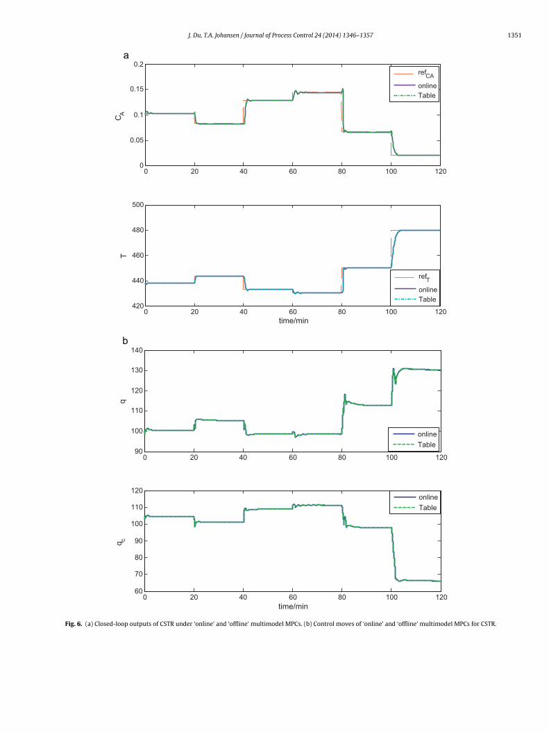

J. Du, T.A. Johansen / Journal of Process Control 24 (2014) 1346–1357 1351

0 20 40 60 80 100 1200

0.05

0.1

0.15

0.2

CA

0 20 40 60 80 100 120420

440

460

480

500

time/min

T

refT

online

Table

refCA

online

Table

0 20 40 60 80 100 12090

100

110

120

130

140

q

0 20 40 60 80 100 12060

70

80

90

100

110

120

time/min

qc

online

Table

online

Table

a

b

Fig. 6. (a) Closed-loop outputs of CSTR under ‘online’ and ‘offline’ multimodel MPCs. (b) Control moves of ‘online’ and ‘offline’ multimodel MPCs for CSTR.

1352 J. Du, T.A. Johansen / Journal of Process Control 24 (2014) 1346–1357

0 20 40 60 80 100 1200

0.05

0.1

0.15

0.2

CA

0 20 40 60 80 100 120420

440

460

480

500

time/min

T

refCA

ke=1

ke=6

refT

ke=1

ke=6

0 20 40 60 80 100 12080

100

120

140

160

q

0 20 40 60 80 100 12060

80

100

120

time/min

qc

ke=1

ke=6

ke=1

ke=6

a

b

F ing pp

msvidtm

ig. 7. (a) Closed-loop outputs of CSTR under multimodel MPCs with different tunarameters.

In the steady state equations of CSTR (11), a pair of (q, qc) deter-ines a single pair of (CA, T), while a pair of (CA, T) corresponds to

everal pairs of (q, qc). Therefore, q and qc are selected as schedulingariables for uniqueness. So the scheduling space (also operat-

ng space) is = {(q, qc)|q ∈ [95, 150], qc ∈ [60, 110]}. In order toesign a multimodel predictive controller for this MIMO CSTR sys-em, local linear models are chosen according to the systematic

ethod proposed in [6] with a threshold value 0.6. Three local linear

arameters. (b) Control moves of multimodel MPCs for CSTR with different tuning

models are obtained and their operating points are displayed inTable 2.

The local linear models are displayed as follows in the discretestate-space form with sampling interval Ts = 0.1:

{

�x(k + 1) = Ai�x(k) + Bi�u(k)

�y(k) = Ci�x(k) + Di�u(k), i = 1, 2, 3

J. Du, T.A. Johansen / Journal of Process Control 24 (2014) 1346–1357 1353

0 20 40 60 80 100 1200

0.2

0.4

0.6

0.8

w1

0 20 40 60 80 100 1200

0.5

1

w2

0 20 40 60 80 100 1200

0.5

1

time/min

w3

ke=1

ke=6

ke=1

ke=6

ke=1

ke=6

Fig. 8. Weights of the three local controllers for the MIMO CSTR system.

0 20 40 60 80 100 12090

100

110

120

130

140

150

u1

0 20 40 60 80 100 12060

70

80

90

100

110

120

u2

time/min

u11

u21

u31

u12

u22

u32

Fig. 9. Control moves of the three local controllers for the MIMO CSTR system with ke = 1.

1354 J. Du, T.A. Johansen / Journal of Process Control 24 (2014) 1346–1357

0 20 40 60 80 100 12010

20

30

40

50

60

70

80

w x

u1

0 20 40 60 80 100 12010

20

30

40

50

60

time/min

w x

u2

w1 x u

12

w2 x u

22

w3 x u

32

w1 x u

11

w2 x u

21

w3 x u

31

the gl

[[[[

eamustb

5

epsFtwoiTi

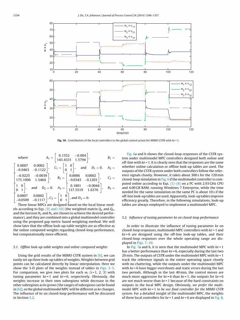
Fig. 10. Contribution of the local controllers to

where A1 =[

0.1552 −0.004143.4331 1.5794

], B1 =

0.0007 0.0002−0.0463 −0.1122

], C1 =

[1 00 1

], and D1 = 0. A2 =

−0.0225 −0.0039175.1096 1.5464

], B2 =

[0.0006 0.0002

−0.0343 −0.1203

], C2 =

1 00 1

], and D2 = 0. A3 =

[0.1801 −0.0044

137.5519 1.6376

], B3 =

0.0007 0.0002−0.0509 −0.1117

], C3 =

[1 00 1

], and D3 = 0.

Three linear MPCs are designed based on the local linear mod-ls according to Eqs. (9) and (10) (the weighted matrix Qy and Qu,nd the horizon Ny and Nu are chosen to achieve the desired perfor-ance), and they are combined into a global multimodel controller

sing the proposed gap metric based weighting method. We willhow later that the offline look-up-table weights are as effective ashe online computed weights regarding closed-loop performance,ut computationally more efficient.

.1. Offline look-up-table weights and online computed weights

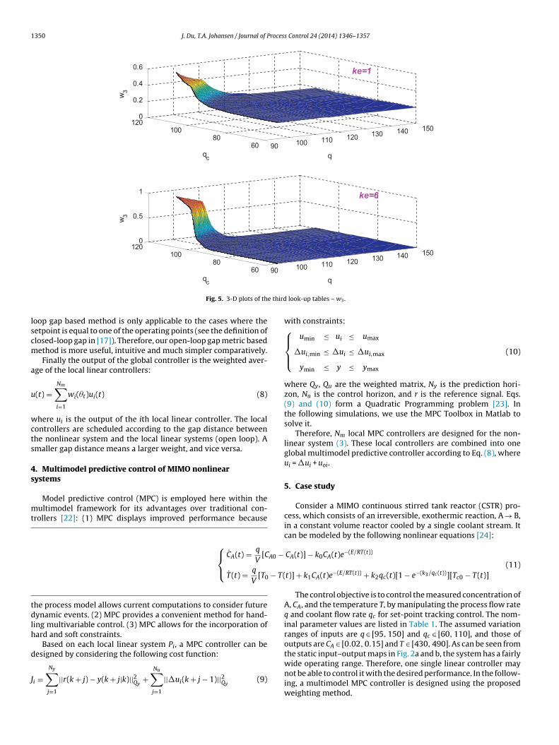
Using the grid results of the MIMO CSTR system in [6], we canasily set up three look-up tables of weights. Weights between gridoints can be calculated directly by linear interpolation. Here wehow the 3-D plots of the weights instead of tables in Figs. 3–5.or comparison, we give two plots for each wi (i = 1, 2, 3) withuning parameter ke = 1 and ke = 6, respectively. Obviously, theeights increase in their own subregions while decrease in the

ther subregions as ke grows (the ranges of subregions can be foundn [6]), so the global multimodel MPC will be different as ke changes.he influence of ke on closed-loop performance will be discussedn Section 5.2.

obal control action for MIMO CSTR with ke = 1.

Fig. 6a and b shows the closed-loop responses of the CSTR sys-tem under multimodel MPC controllers designed both online andoff-line with ke = 1. It is clearly seen that the responses are the samewhether online calculation or offline look-up tables are used. Theoutputs of the CSTR system under both controllers follow the refer-ence signals closely. However, it takes about 300 s for the 120 minclosed-loop simulation in Fig. 6 if the multimodel controller is com-puted online according to Eqs. (5)–(8) on a PC with 2.93 GHz CPUand 4.00 GB RAM, running Windows 7 Enterprise, while the timeneeded for the same simulation on the same PC is about 10 s if theoff-line look-up tables are used. Apparently, look-up tables improveefficiency greatly. Therefore, in the following simulations, look-uptables are always employed to implement a multimodel MPC.

5.2. Influence of tuning parameter ke on closed-loop performance

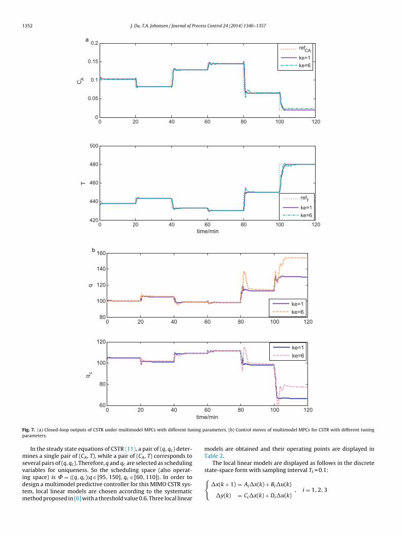
In order to illustrate the influence of tuning parameter ke onclosed-loop responses, multimodel MPC controllers with ke = 1 andke = 6 are designed using the off-line look-up tables, and theirclosed-loop responses over the whole operating range are dis-played in Figs. 7–10.

In Fig. 7a and b, it is seen that the multimodel MPC with ke = 1has a better performance than ke = 6, especially during the last two20 min. The outputs of CSTR under the multimodel MPC with ke = 1track the reference signals in the entire operating space closelywith no chattering, while the outputs under the multimodel MPCwith ke = 6 have bigger overshoots and static errors during the lasttwo periods. Although in the last 40 min, the control moves aremuch more aggressive for ke = 6 than ke = 1, the outputs for ke = 6are not much worse than ke = 1 because of the hard constraints on

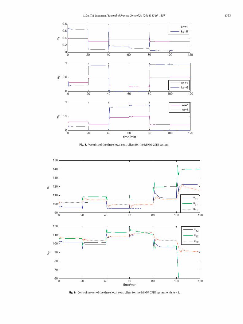
outputs in the local MPC design. Obviously, we prefer the multi-model MPC with ke = 1 to be our final controller for the MIMO CSTRsystem. For a detailed insight of the multimodel MPC, the weightsof three local controllers for ke = 1 and ke = 6 are displayed in Fig. 8,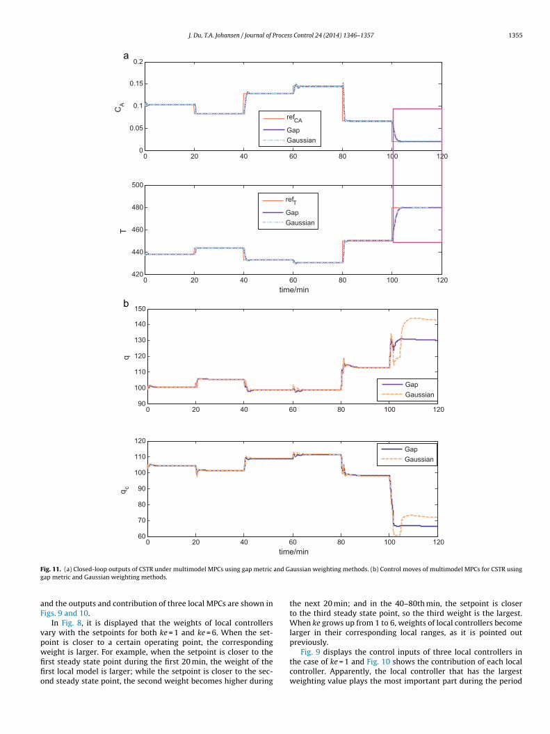

J. Du, T.A. Johansen / Journal of Process Control 24 (2014) 1346–1357 1355

0 20 40 60 80 100 12090

100

110

120

130

140

150

q

0 20 40 60 80 100 12060

70

80

90

100

110

120

time/min

qc

Gap

Gaussian

Gap

Gaussian

0 20 40 60 80 100 1200

0.05

0.1

0.15

0.2

CA

0 20 40 60 80 100 120420

440

460

480

500

time/min

T

refT

Gap

Gaussian

refCA

Gap

Gaussian

a

b

F and Gg

aF

vpwfifio

ig. 11. (a) Closed-loop outputs of CSTR under multimodel MPCs using gap metric

ap metric and Gaussian weighting methods.

nd the outputs and contribution of three local MPCs are shown inigs. 9 and 10.

In Fig. 8, it is displayed that the weights of local controllersary with the setpoints for both ke = 1 and ke = 6. When the set-oint is closer to a certain operating point, the corresponding

eight is larger. For example, when the setpoint is closer to therst steady state point during the first 20 min, the weight of therst local model is larger; while the setpoint is closer to the sec-nd steady state point, the second weight becomes higher during

aussian weighting methods. (b) Control moves of multimodel MPCs for CSTR using

the next 20 min; and in the 40–80th min, the setpoint is closerto the third steady state point, so the third weight is the largest.When ke grows up from 1 to 6, weights of local controllers becomelarger in their corresponding local ranges, as it is pointed outpreviously.

Fig. 9 displays the control inputs of three local controllers inthe case of ke = 1 and Fig. 10 shows the contribution of each localcontroller. Apparently, the local controller that has the largestweighting value plays the most important part during the period

1356 J. Du, T.A. Johansen / Journal of Process Control 24 (2014) 1346–1357

100 102 104 106 108 110 112 114 116 118 120

0

0.02

0.04

0.06

CA

100 102 104 106 108 110 112 114 116 118 120

450

460

470

480

tim

T

refT

Gap

Gaussian

refCA

Gap

Gaussian

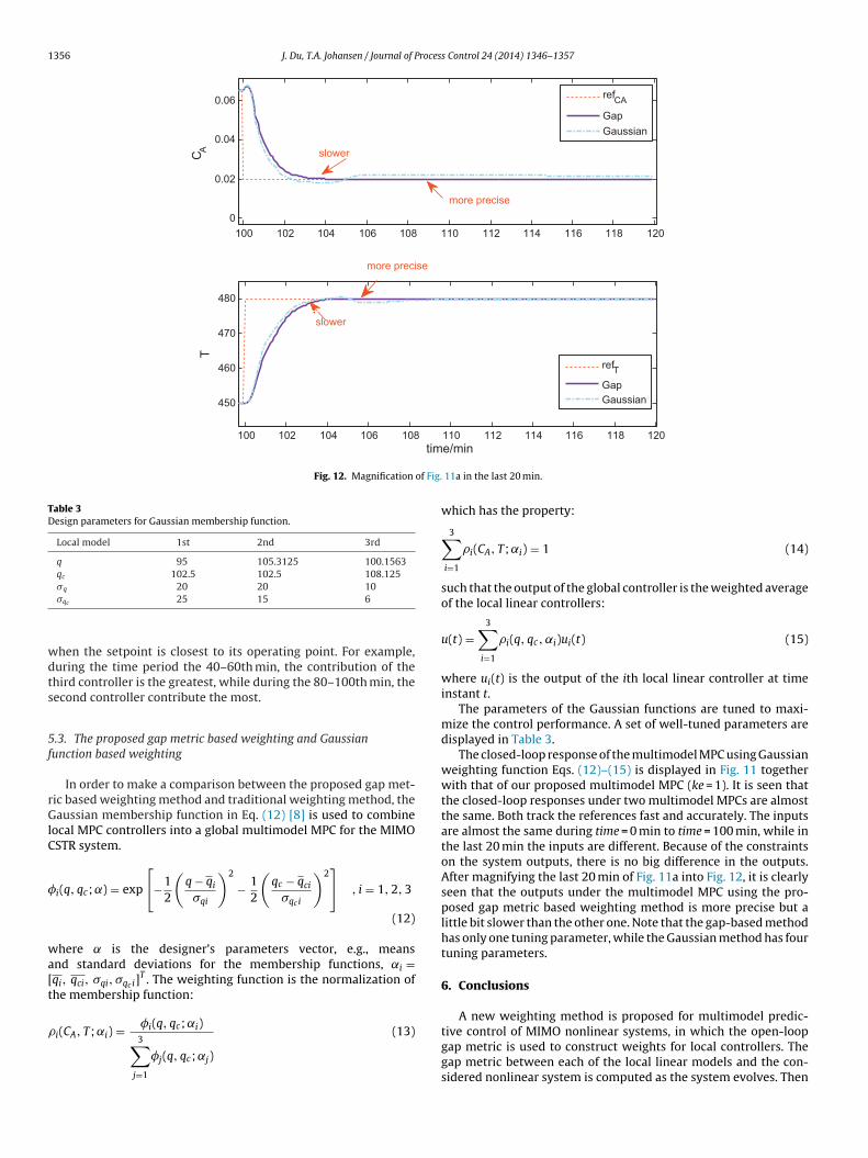
more precise

slower

slower

more precise

Fig. 12. Magnification of Fig.

Table 3Design parameters for Gaussian membership function.

Local model 1st 2nd 3rd

q 95 105.3125 100.1563qc 102.5 102.5 108.125� 20 20 10

wdts

5f

rGlC

�

wa[t

� tive control of MIMO nonlinear systems, in which the open-loop

q

�qc 25 15 6

hen the setpoint is closest to its operating point. For example,uring the time period the 40–60th min, the contribution of thehird controller is the greatest, while during the 80–100th min, theecond controller contribute the most.

.3. The proposed gap metric based weighting and Gaussianunction based weighting

In order to make a comparison between the proposed gap met-ic based weighting method and traditional weighting method, theaussian membership function in Eq. (12) [8] is used to combine

ocal MPC controllers into a global multimodel MPC for the MIMOSTR system.

i(q, qc; ˛) = exp

[−1

2

(q − qi

�qi

)2

− 12

(qc − qci

�qci

)2]

, i = 1, 2, 3

(12)

here is the designer’s parameters vector, e.g., meansnd standard deviations for the membership functions, ˛i =qi, qci, �qi, �qci]

T . The weighting function is the normalization ofhe membership function:

i(CA, T; ˛i) = �i(q, qc; ˛i) (13)

3∑

j=1

�j(q, qc; ˛j)

e/min

11a in the last 20 min.

which has the property:

3∑i=1

�i(CA, T; ˛i) = 1 (14)

such that the output of the global controller is the weighted averageof the local linear controllers:

u(t) =3∑

i=1

�i(q, qc, ˛i)ui(t) (15)

where ui(t) is the output of the ith local linear controller at timeinstant t.

The parameters of the Gaussian functions are tuned to maxi-mize the control performance. A set of well-tuned parameters aredisplayed in Table 3.

The closed-loop response of the multimodel MPC using Gaussianweighting function Eqs. (12)–(15) is displayed in Fig. 11 togetherwith that of our proposed multimodel MPC (ke = 1). It is seen thatthe closed-loop responses under two multimodel MPCs are almostthe same. Both track the references fast and accurately. The inputsare almost the same during time = 0 min to time = 100 min, while inthe last 20 min the inputs are different. Because of the constraintson the system outputs, there is no big difference in the outputs.After magnifying the last 20 min of Fig. 11a into Fig. 12, it is clearlyseen that the outputs under the multimodel MPC using the pro-posed gap metric based weighting method is more precise but alittle bit slower than the other one. Note that the gap-based methodhas only one tuning parameter, while the Gaussian method has fourtuning parameters.

6. Conclusions

A new weighting method is proposed for multimodel predic-

gap metric is used to construct weights for local controllers. Thegap metric between each of the local linear models and the con-sidered nonlinear system is computed as the system evolves. Then

roces

tstccmto[iltoa

tmtelp

A

BrFn(o

R

[

[

[

[

[

[

[

[

[

[

[

[

[

[23] J.M. Maciejowski, Predictive Control with Constraints, Pearson Education

J. Du, T.A. Johansen / Journal of P

he gaps are used to formulate weights of local MPC controllers,uch that large gap means low weight. Finally the global con-roller is made up of a weighted combination of the local MPControllers using the gap-constructed weights. Compared to theurrent methods, the proposed weighting method is easier andore effective: comparing with Gaussian or Trapezoidal func-

ions, our method is significantly simpler since there is onlyne tuning parameter. Comparing with the weighting method in17], our method is independent of controller parameters, ands applicable to constrained MPC which is superior in control-ing MIMO chemical processes. A MIMO CSTR process is studiedo demonstrate the proposed weighting method. The outputsf the controlled system are smooth and output chattering isvoided.

The proposed weighting functions are calculated by linearizinghe nonlinear system. If the process model is not available, a proper

odel should be identified before applying the proposed method. Ifhe process model is not accurate or the plant operates far from thequilibrium, the weighting method might not work or the closed-oop performance may deteriorate. Future work will focus on suchroblems.

cknowledgments

This work was carried out during the tenure of an ERCIM “Alainensoussan” Fellowship Programme. The research leading to theseesults has received funding from the European Union Seventhramework Programme (FP7/2007-2013) under grant agreement◦ 246016, and this work was partly supported by the NSF61104079) of China, and partly by the Doctors’ Funds (B2011-007)f Henan Polytechnic University.

eferences

[1] R. Murray-Smith, T.A. Johansen, Multiple Model Approaches to Modelling andControl, Taylor & Francis, London, England, 1997.

[2] A. Banerjee, Y. Arkun, Model predictive control of plant transitions using a newidentification technique for interpolation nonlinear models, J. Process Control8 (4–6) (1998) 441–457.

[3] Q. Chen, L. Gao, R.A. Dougal, S. Quan, Multiple model predictive control for ahybrid proton exchange membrane fuel cell system, J. Power Sources 19 (2009)472–482.

[4] J.A. Rodriguez, J.A. Romagnoli, G.C. Goodwin, Supervisory multiple regime con-trol, J. Process Control 13 (2003) 177–191.

[

s Control 24 (2014) 1346–1357 1357

[5] N.N. Nandola, S. Bhartiya, A multiple model approach for predictive control ofnonlinear hybrid systems, J. Process Control 18 (2008) 131–148.

[6] J. Du, C. Song, Y. Yao, P. Li, Multilinear model decomposition of MIMO nonlin-ear systems and its implication for multilinear model-based control, J. ProcessControl 23 (2013) 271–281.

[7] K.A. Kosanovich, J.G. Charboneau, M.J. Piovoso, Operating regime-based con-troller strategy for multi-product processes, J. Process Control 7 (1) (1997)42–56.

[8] F. Azimzadeh, O. Galan, J.A. Romagnoli, On-line optimal trajectory control for afermentation process using multi-linear models, Comput. Chem. Eng. 25 (2001)15–26.

[9] J. Novak, V. Bobal, Predictive control of the heat exchanger using local modelnetwork, in: 17th Mediterranean Conference on Control & Automation, Make-donia Palace, Thessaloniki, Greece, 2009.

10] O. Galán, J.A. Romagnoli, A. Palazoglu, Y. Arkun, Gap metric concept and impli-cation for multilinear model-based controller design, Ind. Eng. Chem. Res. 42(2003) 2189–2197.

11] B.A. Foss, T.A. Johansen, A.V. Sorensen, Nonlinear predictive control using localmodels-applied to a batch fermentation process, Control Eng. Pract. 3 (3) (1995)389–396.

12] W. Tan, H.J. Marquez, T. Chen, J. Liu, Multimodel analysis and con-troller design for nonlinear processes, Comput. Chem. Eng. 28 (2004)2667–2675.

13] C. Yu, R.J. Roy, H. Kaufman, B.W. Bequette, Mutiple-model adaptive predictivecontrol of mean arterial pressure and cardiac output, IEEE Trans. Biomed. Eng.39 (8) (1992) 764–778.

14] B. Aufderheide, B.W. Bequette, Extension of dynamic matrix control of multiplemodels, Comput. Chem. Eng. 27 (2003) 1079–1096.

15] J. Du, C. Song, P. Li, Multimodel control of nonlinear systems: an integrateddesign procedure based on gap metric and H∞ loop-shaping, Ind. Eng. Chem.Res. 51 (2012) 3722–3731.

16] J. Du, C. Song, P. Li, A gap metric based nonlinearity measure for chemical pro-cesses, in: Proceedings of 2009 American Control Conference, St. Louis, MO,USA, 2009, pp. 4440–4445.

17] E. Arslan, M.C. Camurdan, A. Palazoglu, Y. Arkun, Multimodel scheduling con-trol of nonlinear systems using gap metric, Ind. Eng. Chem. Res. 43 (2004)8274–8283.

18] G.T. Tan, On Measuring Closed-Loop Nonlinearity: A Topological ApproachUsing the v-Gap Metric (PhD thesis), University of British Columbia, Vancouver,Canada, 2004.

19] T.T. Georgiou, M.C. Smith, Optimal robustness in the gap metric, IEEE Trans.Autom. Control 35 (6) (1990) 673–686.

20] A.K. El-Sakkary, The gap metric: robustness of stabilization of feedback systems,IEEE Trans. Autom. Control 30 (3) (1985) 240–247.

21] W.J. Rugh, J.S. Shamma, Research on gain scheduling, Automatica 36 (2000)1401–1425.

22] D. Dougherty, D. Cooper, A practical multiple model adaptive strategy forsingle-loop MPC, Control Eng. Pract. 11 (2003) 141–159.

Limited, Prentice Hall, London, 2002.24] M.A. Garcia-Alvarado, I.I. Ruiz-Lopez, A design method for robust and

quadratic optimal MIMO linear controllers, Chem. Eng. Sci. 65 (2010)3431–3438.