Journal of

Mechanics ofMaterials and Structures

INDENTATION ANALYSIS OF FRACTIONAL VISCOELASTICSOLIDS

Rouzbeh Shahsavari and Franz-Josef Ulm

Volume 4, Nº 3 March 2009

mathematical sciences publishers

JOURNAL OF MECHANICS OF MATERIALS AND STRUCTURESVol. 4, No. 3, 2009

INDENTATION ANALYSIS OF FRACTIONAL VISCOELASTIC SOLIDS

ROUZBEH SHAHSAVARI AND FRANZ-JOSEF ULM

The constitutive differential equations governing the time-dependent indentation response for axisymet-ric indenters into a fractional viscoelastic half-space are derived, together with indentation creep andrelaxation functions suitable for the backanalysis of fractional viscoelastic properties from indentationdata. These novel fractional viscoelastic indentation relations include, as a subset, classical integer-typeviscoelastic models such as the Maxwell model or Zener model. Using the correspondence principleof viscoelasticty, it is found that the differential order of the governing equations of the indentationresponse is higher than the one governing the material level. This difference in differential order betweenthe material scale and indentation scale is more pronounced for the viscoelastic shear response than forthe viscoelastic bulk response, which translates, into fractional derivatives, the well-known fact that anindentation test is rather a shear test than a hydrostatic test. By way of example, an original method for theinverse analysis of fractional viscoelastic properties is proposed and applied to experimental indentationcreep data of polystyrene. The method is based on fitting the time-dependent indentation data (in theLaplace domain) to the fractional viscoelastic model response. Applied to polysterene, it is shown thatthe particular time-dependent response of this material is best captured by a bulk-and-deviator fractionalviscoelastic model of the Zener type.

1. Introduction

The aim of indentation analysis is to link indentation data, typically an indentation force versus inden-tation depth curve, F-h, to meaningful mechanical properties of the indented material. It is commonpractice to condense the indentation data into two quantities, the hardness H and the indentation modulusM , which are related to measured indentation data, namely the maximum indentation force Fmax, theinitial slope (or indentation stiffness) S of the unloading curve, and the projected contact area Ac by

H def=

Fmax

Ac, S =

d Fdh|h=hmax

def=

2√π

M√

Ac. (1)

Traditionally, for metals, the hardness H was early on recognized to relate to strength properties ofthe indented material [Brinell 1901; Tabor 1951], and recent developments in indentation analysis haveextended those approaches to account for strain hardening [Cheng and Cheng 2004], cohesive-frictionalstrength behavior [Ganneau et al. 2006], and the effect of porosity on the strength behavior [Cariou et al.2008]. The investigation of the link between the unloading slope S and the elasticity properties of theindented material is more recent, requiring depth sensing indentation techniques that provide a continuous

Keywords: fractional viscoelasticity, indentation analysis, creep, relaxation, correspondence principle, polysterene.This work was supported by Schoettler Fellowship Program at MIT, and Schlumberger–Doll Research, Cambridge, MA. Theexperimental data on Polystyrene was provided by Dr. Catherine Tweedie and Prof. Krystyn J. Van Vliet, of MIT’s Departmentof Material Science and Engineering.

523

524 ROUZBEH SHAHSAVARI AND FRANZ-JOSEF ULM

Indenter shape n B φ F-h relation

Cone 1 cot θ 2 tan θπ

F = 2M tan θπ

h2

Sphere 2 1/2R 4√

R3

F = 4M√

R3

h1.5

Flat punch →∞ 1/an 2a F = 2Mah

Table 1. F-h equations for different indenter shapes. θ is the half-cone angle, R and aare the sphere radius and the flat cylinder punch, respectively.

record of the F-h curve during loading and unloading in an indentation test [Tabor 1951; Doerner andNix 1986; Oliver and Pharr 1992; Bulychev 1999]. Relation (1)2 is an exact relation for linear elasticmaterials. For non-elastic materials, (1)2 becomes an approximate relation and S may be affected by theresidual stress field and by adhesion of materials [Borodich and Galanov 2008]. Application of the depthsensing indentation techniques in indentation analysis confirmed the link provided by classical linearelastic contact mechanics solutions [Hertz 1882; Boussinesq 1885; Love 1939; Galin 1961; Sneddon1965; Borodich and Keer 2004] for a rigid indenter of axysmmetric shape that can be described by amonomial function of the form z = Brn:

F = φMh1+1/n, (2)

where r and z are, respectively, the first and the third cylindrical coordinates of the surface of the tip, φ(of dimension [φ] = L1−1/n), condenses the indenter specific geometry parameters,

φ =2

(√πB)1/n

nn+ 1

[0(n/2+ 1/2)0(n/2+ 1)

]1/n, (3)

B is the shape function of the indenter at unit radius, n ≥ 0 is the degree of the homogeneous function,0(x) is the Euler Gamma function, 0(x)=

∫∞

0 t x−1 exp(−t)dt . Table 1 develops expression (2) for somecommon indenter shapes. Finally, M is the indentation modulus. The indentation modulus M provides asnapshot of the elasticity of the indented material. In the isotropic case, M relates to the bulk and shearmodulus (K ,G) of the indented half-space by

M = 4G3K +G

3K + 4G. (4)

Based on the adaptation for indentation analysis of the method of functional equations [Lee and Radok1960], closed-form solutions for indentation in various linear viscoelastic solids became recently availablefor a variety of indenter shapes: flat punch indentation [Cheng et al. 2000], spherical indentation [Chenget al. 2005; Oyen 2005], and conical indentation [Vandamme and Ulm 2006; Oyen 2006], which havebeen synthesized into viscoelastic indentation creep and relaxation functions for any indenter of axysm-metric shape [Vandamme and Ulm 2007]. Those linear viscoelastic approaches are relevant for materialswhose behavior can be described by the classical integer-type time-dependent differential equation of

INDENTATION ANALYSIS OF FRACTIONAL VISCOELASTIC SOLIDS 525

linear viscoelasticity [Bland 1960],

σ +

I∑i=1

Pid iσ

dt i = E ′(ε+

J∑j=1

Q jd jε

dt j

), (for i = 1, 2, . . . I ; j = 1, 2, . . . J ), (5)

where σ and ε are stress and strain, Pi and Q j stand for relaxation and retardation time, respectively,and E ′ is the relaxed elasticity modulus. The restriction to integer-type time derivatives to describethe ‘real’ stress relaxation and creep behavior of polymers and other materials has been recognized asa drawback for material characterization [Rossikhin and Shitikova 2004] and can be removed by theintroduction of fractional derivatives in the time-dependent differential equation. The application offractional viscoelastic material models in indentation analysis is the focus of this paper. The paper isstructured as follows: Following a brief review of the basic concepts of fractional derivatives, we derive ageneral differential representation of the time-dependent indentation response of a fractional viscoelasticmaterial half-space using the correspondence principle. The general solution is then adapted to derivecreep and relaxation functions that potentially allow the determination of meaningful viscous materialproperties from time-dependent experimental indentation data.

2. Elements of fractional order derivatives

Fractional calculus is an old mathematical topic, but its application in physics and engineering is morerecent. For instance, in viscoelasticity and hereditary solid mechanics [Bagley and Torvik 1983], elec-tromagnetic systems [Engheta 1996], and diffusion phenomena in inhomogeneous media [Arkhincheev1993] , fractional order derivatives have been used to describe the system behavior. From a mathematicalperspective, fractional derivatives are an extension of ordinary derivatives, and possess mathematicaldefinitions and properties that stem from ordinary derivatives. Some definitions of fractional derivativescan be found in [Podlubny 1999] and [Kilbas et al. 2006]. The Riemann–Liouville definition is thesimplest one. According to this definition, the α-th order fractional derivative of a function f (t) withrespect to t is

Dα f (t)=∂α

∂tαf (t)=

10(m−α)

∂m

∂tm

∫ t

a

f (τ )(t − τ)α+1−m dτ, m− 1≤ α < m, (6)

where m is the first integer larger than α, and a is the lower limit related to the operation of fractionaldifferentiation. Following [Ross 1977], we call a the lower terminal value and set a = 0 for all fractionaldefinitions in this article. We also use the short hand notation Dα f (t)= ∂α

∂tα f (t). The Laplace transformof the Riemann–Liouville derivative is given by

Dα f (t)= sα f (s)−m−1∑k=0

sk Dα−k−1 f (0), m− 1≤ α < m, (7)

where s is the Laplace parameter and f (s) stands for the Laplace transform of f (t). Applying thisdefinition to solve initial value problems requires knowledge of the non-integer derivatives of the initialconditions at t = 0. Despite the fact that mathematically these problems can be solved successfully,their solution is practically meaningless because there is no physical interpretation available for such

526 ROUZBEH SHAHSAVARI AND FRANZ-JOSEF ULM

initial conditions. A solution to this conflict was proposed by Caputo [1967; 1969]. Caputo’s fractionalderivative (for a zero terminal value) can be written as

Dα f (t)=1

0(m−α)

∫ t

0

f (m)(τ )(t − τ)α+1−m dτ, m− 1< α < m, (8)

where f (m)(τ )= ∂m

∂τm f (τ ). The Laplace transform of (8) is given by

Dα f (t)= sα f (s)−m−1∑k=0

sα−1−k f (k)(0), m− 1< α ≤ m, (9)

where in (9), only ordinary derivatives are acted upon initial conditions. Another main difference betweenthe two definitions is that the Caputo derivative (8) of a constant C is zero,

DαC = 0, (10)

whereas in the cases of a finite lower terminal value, the Riemann–Liouville fractional derivative (6) ofa constant C is not zero but is given by [Podlubny 1999]

DαC =Ct−α

0(1−α). (11)

It can be shown that for α→ m, Caputo’s fractional derivative becomes a conventional m-th derivative[Podlubny 1999; Kilbas et al. 2006],

Dα f (t)= f (m)(t). (12)

Similar to integer-order differentiation, Caputo’s fractional differentiation is a linear operation,

Dα(λ f (t)+µg(t)

)= λDα f (t)+µDαg(t), (13)

where λ and µ are constants. Analogous to [Schiessel et al. 1995], by using Caputo’s fractional deriv-ative, the well-known Hookian spring relation, σ(t)= Eε(t), and Newtonian dashpot relation, σ(t)=η dε(t)/dt , can be generalized to

σ(t)= Eταdαε(t)

dtα= EταDαε(t), 0< α < 1. (14)

In (14), the parameter τ with units of time is employed to non-dimensionalize the fractional derivative ofε, which helps to obtain a meaningful physical relation between stress and strain. Note that here, since0< α < 1, Eq (8) reduces to

Dα f (t)=1

0(1−α)

∫ t

0

f (1)(τ )(t − τ)α

dτ, 0< α < 1. (15)

Throughout this work, we will exclusively refer to Caputo’s definition when using the term fractionalderivatives. A full discussion on differences between Caputo and Riemann–Liouville fractional deriva-tives, and the conditions when they both become equivalent, can be found in [Podlubny 1999]. Theintroduction of the integrodifferential operator (15) in (14) offers a number of interesting perspectivesfor modeling viscoelastic behavior. From a mathematical perspective, due to the convolution with t−α,σ(t) has a fading memory [Baker et al. 1996]. To illustrate this behavior, consider a simple rod in uniaxial

INDENTATION ANALYSIS OF FRACTIONAL VISCOELASTIC SOLIDS 527

α = 0 No memory α = 1 Perfect memory 0< α < 1 Partial memory

σ = Eτ 0 ∂0ε∂t0 = Eε σ = Eτ ∂

1ε∂t1 = η

∂1ε∂t1 σ = Eτα ∂

αε∂tα

Figure 1. Illustration of integer and fractional models.

extension by a strain ε. In the limit cases, if α = 0, Dαε = ε, and if α = 1, Dαε = ε (this can be provedby integration by parts). Thus, by multiplying a constant, Eτα, to Dαε, depending on the value of α,one obtains either the elastic force (spring model) or the damping force (dashpot model). In other words,α = 0 corresponds to a system with no memory since the stress depends only on the instantaneousmagnitude of ε (Figure 1, left), while α = 1 corresponds to a system with perfect memory since thetime history and the particular way the system has reached its current position becomes important forderivative calculations (Figure 1, middle). For any 0 < α < 1, the system has partial memory, andconsequently the derived stress is a combination of dashpot and spring models (symbolized by a squarein Figure 1, right). Relative to discrete (integer) derivatives, therefore, fractional derivatives offer a widerange for modeling the rate of change of the time-dependent behavior of viscoelastic materials in acontinuous fashion. Figure 2 displays a simple function along with its half-derivative and first derivative,showing that fractional derivatives are usually sandwiched in between the closest lower and upper integer-derivatives. This allows one to monitor changes in a much smoother and compact fashion than offeredby integer derivatives.

While spring and dashpot models can be recognized by only one material property parameter (E and η,respectively), introducing a fractional element requires three parameters, called α, τ , and E . A fractionalelement with only three parameters is mathematically and physically equivalent to an infinite number ofsimple springs and dashpots connected through a certain hierarchical arrangement [Schiessel and Blumen1993]. Thus, capturing the continuous rate of change in time by means of integer-type models requires

0 1 2 3 4 5 60

1

2

3

4

5

6 D0 f = f

D1/2 f = g, g(x)= 2√

x/π

D1 f = 1

Figure 2. Derivatives of f (x)= x of order 0 (black), 12 (red) and 1 (blue).

528 ROUZBEH SHAHSAVARI AND FRANZ-JOSEF ULM

),,( 2Etg

1E

0E

F

h

G

G

Figure 3. Fractional Zener model with identical fractional order derivatives on stressand strain.

generally many higher integer-order derivative terms in (5) to achieve a similar accuracy. With the abovepreliminary explanations, the extension of (5) to fractional derivatives can be written as

σ +

I∑i=1

Piταi Dαiσ = E ′

(ε+

J∑j=1

Qτβ j Dβ j ε), (for i = 1, 2, . . . I ; j = 1, 2, . . . J ), (16)

where αi , β j ∈ [0, 1]. Each fractional term in (16) can be considered as a replacement of a system madeof many conventional springs and dashpots.

By way of application, consider a fractional Zener viscoelastic material, shown in Figure 3, in whichthe dashpot of the conventional Zener model is replaced by a fractional element. As shown below, thismodel is described by a fractional differential equation in which only the first fractional derivative terms(I = J = 1) are present in each series in (16), and in which the fractional derivative of stress and strain isidentical (α1 = β1). There are five independent parameters in this model, called E0, E1, E2, γ, τ . Indeed,the total strain on the right branch is

ε = εs + ε f , (17)

where subscripts s, f refer to the spring element and the fractional element, respectively. As theseelements are connected in series, their stresses are equal,

σR = E1εs = E2τγ Dγ ε f . (18)

We now take advantage of the linearity property of the fractional operator (13). By taking the γ -thderivative of (17) and using (18) (assuming E1, E2 and τ are constants), we obtain

σR +E2τ

γ

E1Dγ σR = E2τ

γ Dγ ε, (19)

where we let

τ0 =

(E2τγ

E1

)1/γ, S = E2

( ττ0

)γ. (20)

Equation (19) simplifies toσR + τ

γ0 Dγ σR = Sτ γ0 Dγ ε. (21)

INDENTATION ANALYSIS OF FRACTIONAL VISCOELASTIC SOLIDS 529

Equation (21), which describes the behavior of the right branch of the model in Figure 3, turns out to bethe constitutive fractional differential equation of a Maxwell model in which the conventional dashpot isreplaced by the fractional element.

The total stress in the parallel system is

σ = σL + σR, (22)

where σL is the elastic stress in the left branch of the model displayed in Figure 3

σL = E0ε. (23)

Then, take the γ -th derivative of (22) and multiply the result with τ γ0 :

τγ0 Dγ σ = τ

γ0 Dγ σL + τ

γ0 Dγ σR. (24)

Finally, by adding (24) and (22), and using (23) and (21), we obtain

σ + τγ0 Dγ σ = E0ε+ (E0+ S)τ γ0 Dγ ε. (25)

Equation (25) is recognized as the one-dimensional constitutive equation of the fractional Zener modelshown in Figure 3. It is characterized by identical fractional order derivatives on stress and strain. This isan important requirement for thermodynamic stability of the model described by (25).1 More generalizedconstitutive equations including different fractional order derivatives on stress and strain can be found in[Schiessel et al. 1995]. In what follows, we employ the fractional Zener model in indentation analysis.

3. Time-dependent indentation response of fractional viscoelastic materials

In general, the time-dependent behavior of hereditary materials, for which the stress depends nonlineralyon the strain history, can be described by the volterra integral equations [Rabotnov 1980]. Most vis-coelastic indentation solutions originate from the method of functional equations developed for linearviscoelastic contact problems by Radok [1957] and completed by Lee and Radok [1960]. The method offunctional equations consists of solving the viscoelastic problem from the elastic solution by replacingthe elastic moduli with their corresponding viscoelastic operators. The method of functional equationscan be seen as an extension of the Laplace transform method, as formulated by Lee [1955]. The Laplacetransform method consists of eliminating the explicit time dependence of the viscoelastic problem byapplying the Laplace transform to the time-dependent moduli and solving the corresponding elasticityproblem in the Laplace domain. The Laplace method, however, is restricted to boundary value problemsin which the displacement and stress boundary conditions are fixed in time. This is generally not thecase in indentation problems (except for the flat punch problem), in which the contact area changes withtime, hence changing a part of the stress boundary outside the contact area into a displacement boundaryinside the contact area and vice versa. This drawback of the Laplace transform was lifted in [Radok1957; Lee and Radok 1960], which introduced and developed the method of functional equations, validfor linear viscoelastic problems with time-dependent boundary conditions. Galanov [1982] established

1There is a special case in which (25), with different fractional derivatives on stress and strain, can be thermodynamicallystable. That is, when the fractional derivative acting on strain is greater than that acting on stress, and only below a certainlimiting frequency [Glöckle and Nonnenmacher 1991].

530 ROUZBEH SHAHSAVARI AND FRANZ-JOSEF ULM

0Q1Q

),,( 2Qvta

1q

),,( 2qdtb

0q

F

hch

q

G

G

Figure 4. A rigid conical indenter on a fractional viscoelastic half-space material (mid-dle) can be studied with a fractional Zener model describing volumetric behavior inindentation (left) or one describing deviatoric behavior in indentation (right).

self-similarity of the contact problem for some viscoelastic solids and gave dimensionless distributionsfor stresses under Vickers and Berkovich indenters. For indentation problems, the method of functionalequations remains valid as long as the contact area (or, equivalently, for viscoelastic materials, the pene-tration depth) increases monotonically [Lee and Radok 1960]. We shall adopt this method for indentationanalysis of fractional viscoelastic materials.

We consider the fractional Zener model shown in Figure 3, whose one-dimensional behavior is de-scribed by (25).2 We employ this model separately for the volumetric and deviatoric part of the three-dimensional stress tensor and strain tensors of the material response to indentation. For the volumetricpart with parameters Q0, Q1, Q2,α, τv, by setting, similarly to (20),

ζv =(Q2τ

αv

Q1

)1/α, K0 = Q2

(τvζv

)α, (26)

the fractional differential equation governing the time-dependent spherical isotropic material responsereads (Figure 4, left),

σv + ζαv Dασv = Q0εv + (Q0+ K0)ζ

αv Dαεv, (27)

where σv = 13(tr σ )1, εv = 1

3(tr ε)1, are the volumetric parts of the second order stress tensor σ and secondorder strain tensor ε, respectively. Similarly, for the deviatoric part with parameters q0, q1,q2, β, τd , bysetting

ζd =

(q2τβd

q1

)1/β, G0 = q2

(τd

ζd

)β, (28)

the fractional differential equation governing the time-dependent deviatoric isotropic material responsereads (Figure 4, right)

σd + ζβd Dβσd = q0εd + (q0+G0)ζ

βd Dβεd . (29)

Here σd and εd are, respectively, the deviatoric parts of the second order stress and strain tensors, σ andε. From basic tensor algebra, relations σ = σv + σd , ε = εv + εd hold. Thus, as Figure 4 shows, based

2For a general nonlinear stress-strain behavior in solids, the fraciotnal calculus can be integrated into the volterra equations[Rabotnov 1980].

INDENTATION ANALYSIS OF FRACTIONAL VISCOELASTIC SOLIDS 531

on our chosen models, there are in total 10 independent parameters Q0, Q1, Q2,α, τv, q0, q1,q2, β, τd

that describe the volumetric and deviatoric material behavior (five for each behavior). For simplicity innotation and avoiding carrying too many parameters in our analytical derivations, we rewrite (27) and(29) as

σv(t)+ P Dασv(t)= Q0εv(t)+ Q Dαεv(t), (30)

σd(t)+ pDβσd(t)= q0εd(t)+ q Dβεd(t), (31)

where we let

P = ζ αv , Q = (Q0+ K0)ζαv , (32)

p = ζ βd , q = (q0+G0)ζβd . (33)

Using (9), the Laplace transforms of (30) and (31) are readily obtained:

(1+ Psα)σv(s)− Psα−1σv(0)= (Q0+ Qsα)εv(s)− Qsα−1εv(0),

(1+ psβ)σd(s)− psβ−1σd(0)= (q0+ qsβ)εd(s)− qsβ−1εd(0),(34)

where σv(s), σd(s), εv(s), εd(s) denote the Laplace transforms of σv(t), σv(t), εv(t), εd(t), whereasσv(0), σd(0), εv(0), εd(0) represent the stress and strain initial conditions at t = 0. We remind ourselvesof the classical Laplace transformations of the stress convolution integrals of linear isotropic viscoelas-ticity [Christensen 1971]:

σv(t)=∫ t

−∞

3K (t − τ)d

dτεv(τ )dτ → σv(s)= 3s K (s)εv(s),

σd(t)=∫ t

−∞

2G(t − τ)d

dτεd(τ )dτ → σd(s)= 2sG(s)εd(s),

(35)

where K (t) and G(t) are the time-dependent bulk and shear modulus, respectively. Then, by comparing(34) and (35), one obtains the following relations for bulk and shear response of the fractional material:

3s K (s)=Q0+ Qsα

1+ Psα, 2sG(s)=

q0+ qsβ

1+ psβ, (36)

andPσv(0)= Qεv(0), pσd(0)= qεd(0). (37)

Equations (37) indicate that the initial conditions acting upon stress and strain are not completely inde-pendent, and relations such as (37) must be satisfied. These constraints do not appear only in fractionalviscoelastic models. Analogous constraints on initial conditions also exist for integer-order viscoelasticmodels [Christensen 1971; Shahsavari and Ostoja-Starzewski 2005].

Similarly, application of the correspondence principle to the elastic indentation modulus M definedby (4) yields [Vandamme and Ulm 2006]

M→ s M(s)= 4sG(s)3s K (s)+ sG(s)

3s K (s)+ 4sG(s). (38)

532 ROUZBEH SHAHSAVARI AND FRANZ-JOSEF ULM

Next, analogously to (35), the application of the correspondence principle of viscoelasticity to theelastic indentation force relation (2) yields

F(t)= φ∫ t

−∞

M(t − τ)d

dτh1+1/n(τ ) dτ H⇒ F(s)= φs M(s) h1+1/n(s). (39)

In (39), we a priori assumed the geometry parameter φ is a time-independent parameter, following [Leeand Radok 1960]. By substituting (36) in (38) and then in (39), one obtains the viscoelastic relation be-tween F(s) and h1+1/n in the transformed Laplace space. Next, by extensively rearranging the terms andusing the relation (9) along with the linearity property (13) for the fractional order terms, the constitutivedifferential equation governing the time-dependent indentation response becomes

DF (F(t))= 2φDh(h1+1/n(t)). (40)

This is a differential equation with constant coefficients involving the operators

DF = c0+ c1 Dα+ c2 Dβ

+ c3 Dα+β+ c4 Dα+2β

+ c5 D2β,

Dh = l0+ l1 Dα+ l2 Dβ

+ l3 Dα+β+ l4 Dα+2β

+ l5 D2β(41)

with coefficients

c0 = Q0+ 2q0, l0 =12q2

0 + q0 Q0,

c1 = Q+ 2Pq0, l1 = q0 Q+ 12 Pq2

0 ,

c2 = 2Q0 p+ 2q + 2pq0, l2 = q0 pQ0+ qq0+ q Q0,

c3 = 2Qp+ 2Pq + 2Ppq0, l3 = q0 pQ+ Pqq0+ q Q,

c4 = Qp2+ 2Ppq, l4 = qpQ+ 1

2 Pq2,

c5 = Q0 p2+ 2pq, l5 = qpQ0+

12q2.

(42)

Note that in view of (37) the following relations between initial conditions hold:

ci F(0)= 2φli�(0), (i = 1, 2, . . . , 5), (43)

ci F (1)(0)= 2φli�(1)(0), (i = 3, 4, 5), (44)

c4 F (2)(0)= 2φl4�(2)(0), (45)

where we have set �(0) = h1+1/n (0). Considering the initial conditions above, the use of Caputo’sderivative results in five integer-order relations in (43) and four inter-order derivatives in (44) and (45).In order for (44) to hold with i = 3, we must have α+ β > 1; the same relation with i = 4 and i = 5requires α+ 2β > 1 and 2β > 1, respectively. Similarly, (45) requires that α+ 2β > 2. If any of theseconditions is not met, the corresponding relation in (44)–(45) does not exist.

The following observations deserve attention:

INDENTATION ANALYSIS OF FRACTIONAL VISCOELASTIC SOLIDS 533

h

G

MhVh

VG

G

Figure 5. Left: Maxwell model. Right: Zener model.

(i) For α = β = 0, which corresponds to the case of a material with no memory (Figure 1, left), Equation(40) reduces to the elastic indentation relation (2), with

M =2l0

c0= 2q0

Q0+12q0

Q0+ 2q0, K =

13

Q0, G =12

q0. (46)

(ii) Letting α = 0 corresponds to the case of a pure deviatoric creep, a case which was extensivelystudied in integer-type viscoelastic indentation analysis (for example, [Cheng and Cheng 2004; Chenget al. 2000; 2005; Vandamme and Ulm 2006]). In this case β = 1, and one obtains(

c0+ (c2+ c3)D1+ (c4+ c5)D2)F(t)= 2φ

(l0+ (l2+ l3)D1

+ (l4+ l5)D2)h1+1/n(t). (47)

Note that a deviatoric creep behavior described at a material level by a first-order differential equation(see (31) for β = 1), yields a second-order differential equation that governs the F(t)− h(t) indentationresponse. This includes, as integer subset models, the three-parameter deviator creep Maxwell modeland the four-parameter deviator creep Kelvin–Voigt or Zener model (Figure 5), for which the constantcoefficients read as follows:

P Q0 Q p q0 q

Maxwell 0 3K 0 ηM/G 0 2ηM

Zener 0 3K 0 ηVG+GV

2 GGVG+GV

2 GG+GV

ηV

(48)

Here ηM and ηV stand for the viscosity in the respective models. Use of (48) in (42) and then in (47)yields the following differential equations for the two particular integer-type viscoelastic models:

Maxwell: F(t)+c2

c0

∂F∂t+

c5

c0

∂2 F∂t2 = 2φ

( l2

c0

∂h1+1/n

∂t+

l5

c0

∂2h1+1/n

∂t2

), (49)

Zener: F(t)+c2

c0

∂F∂t+

c5

c0

∂2 F∂t2 = 2

l0

c0φ(

h1+1/n+

l2

l0

∂h1+1/n

∂t+

l5

l0

∂2h1+1/n

∂t2

). (50)

(iii) The difference in differential order between the material and the indentation scale becomes evenmore apparent for α = β = 1, which converts the fractional model into an integer-type model governed

534 ROUZBEH SHAHSAVARI AND FRANZ-JOSEF ULM

by a third-order differential equation:(c0+(c1+c2)D1

+(c3+c5)D2+c4 D3)F(t) = 2φ

(l0+(l1+l2)D1

+(l3+l5)D2+ l4 D3)h1+1/n(t). (51)

Setting α = β reduces the model to the often considered case of a material with time independentPoisson’s ratio [Gao and Ogden 2003], which is obtained by letting P = p, q = bQ, and q0 = bQ0 forany non-negative value of b in (30)–(31) and (42). This concept is similar to using two same-type integerviscoelastic models with the aforementioned relations between their parameters which lead to a constantPoisson’s ratio [Tschoegl et al. 2002].

(iv) This difference in differential order between the material and the indentation scale holds true forfractional materials; that is, because of the definition of the differential operators in (41), the order of thefractional derivatives at the indentation scale given by (40), is always greater than the one of the materiallevel defined by (30)–(31). For example, for a deviatoric fractional creep model, α = 0, the differentialequation (31) governing the material behavior is of order 0< β < 1, while the indentation response isof order 2β, and can thus be greater than unity:(

c0+ (c2+c3)Dβ+ (c4+c5)D2β)F(t)= 2φ

(l0+ (l2+l3)Dβ

+ (l4+l5)D2β)h1+1/n(t). (52)

The specification of (52) for a fractional deviatoric Maxwell material (P = Q = q0 = 0) and a fractionaldeviatoric Zener material (P = Q = 0) reads as follows:

Maxwell: F(t)+c2

c0

∂βF∂tβ+

c5

c0

∂2βF∂t2β = 2φ

( l2

c0

∂βh1+1/n

∂tβ+

l5

c0

∂2βh1+1/n

∂t2β

), (53)

Zener: F(t)+c2

c0

∂βF∂tβ+

c5

c0

∂2βF∂t2β = 2

l0

c0φ(

h1+1/n+

l2

l0

∂βh1+1/n

∂tβ+

l5

l0

∂2βh1+1/n

∂t2β

), (54)

where the coefficients c0, . . . , c5 and l0, . . . , l5) are still given by (42). Their dimensionality, however,changes due to the application of non-integer time derivatives. For instance, we have [c2/c0] = [l2/ l0] =

T β , while [c5/c0] = [l5/ l0] = T 2β , and so on. Still, analogously to (19)–(20), one can define parameterssimilar to τ0 with the dimension of time and replace the the fractional dimension of c2/c0, etc.

(v) The operators (41) are not symmetric with respect to α and β; that is, in contrast to α, which is thefractional exponent for the volumetric viscoelastic response (30), there are some extra terms that involvehigher derivatives of order 2β, which is the fractional exponent for the viscoelastic shear response (31).This observation translates, into fractional derivatives, the well-known fact that an indentation test is ashear test than a hydrostatic test. For this reason, the effect of β dominates over the effect of α in thefractional derivatives that define the indentation response (40). This dominance of shear over bulk existsfor conventional viscoelastic materials in indentation, but it is hidden in the constitutive equations.

4. Indentation creep and relaxation functions

A convenient way to analyze time-dependent experimental indentation data is in the form of indentationcreep and relaxation functions, derived for a step force loading or step displacement loading, respectively.It is also a formidable illustration of the use of the fractional model developed here before.

INDENTATION ANALYSIS OF FRACTIONAL VISCOELASTIC SOLIDS 535

4.1. Indentation creep compliance. Consider a Heaviside step loading F(t) = FmaxH(t), where Fmax

is the maximum load, and H(t) the Heaviside step function. We recall the Laplace transform F(s) ofthe Heaviside load function:

F(t)= FmaxH(t) ⇐⇒ F(s)=Fmax

s. (55)

Then, a substitution of (55) in (39) along with a substitution of (55) in Laplace transform of (40) can bedeveloped in the form

L(s)=φ h1+1/n(s)

Fmax=

1

s2 M(s)=

DF (s)

2s Dh(s), (56)

where DF (s) and Dh(s) are the Laplace transforms of the operators (41) according to definition (9):3

DF (s)= c0+ c1sα + c2sβ + c3sα+β + c4sα+2β+ c5s2β, (57)

Dh(s)= l0+ l1sα + l2sβ + l3sα+β + l4sα+2β+ l5s2β . (58)

Note that the inverse Laplace transform of (56), L(t), has dimension of compliance [L] = 1/(L−1 MT−2),and can therefore be appropriately called an indentation creep compliance function. As discussed in detailfor integer-type viscoelasticity models in [Vandamme and Ulm 2007], the indentation creep complianceis independent of the indenter-shape. The right-hand side of (56), therefore, is representative of thematerial response of the considered fractional viscoelastic material. The inverse transform of (56) exists,is real, and continuous. The following statements are derived in the Appendix:

(i) For a ‘double’ Zener model (Zener bulk and Zener deviatoric creep model), the inverse Laplacetransform of (56) yields the following expression of the time-dependent indentation creep compliance:

L(t)=φh1+1/n(t)

Fmax

=c0

2l0+

1π

Im∫∞

0

DF (re−iπ )

2re−iπ Dh(re−iπ )exp(−r t) dr +

∑j

lims→λm

j

(s− λmj )

DF (λmj ) exp(λm

j t)

2λmj Dh(λ

mj )

, (59)

where m is the smallest common denominator of the fractional numbers α and β. Note that λm is acomplex number with negative real part. Thus, as t→∞, the second and the third terms on the right-hand side of (59) vanish and L(t) converges to a constant c0/2l0. This is because in Zener-type models(either fractional or integer; see Figure 5, right), there is a spring parallel to the rest of the system thatprevents infinite deformation.

3Initial conditions in the Laplace transform of a derivative of a Heaviside function are zero, since 0− ( and not 0+ ) is takenas a lower limit of Laplace integration for a Heaviside function. More details can be found in [Flügge 1967].

536 ROUZBEH SHAHSAVARI AND FRANZ-JOSEF ULM

(ii) For a ‘double’ Maxwell model, the expression of the inverse Laplace transform is the same one as(59), except for the first term on the right:

L(t)=φh1+1/n(t)

Fmax

=1

2(k− 1)!∂k−1

∂uk−1 [ f (u) exp(um t)]u=0+1π

Im∫∞

0

DF (re−iπ )

2re−iπ Dh(re−iπ )exp(−r t) dr

+

∑j

lims→λm

j

(s− λmj )

DF (λmj ) exp(λm

j t)

2λmj Dh(λ

mj )

, (60)

where k = m(1+β) is an integer, and

f (u)=c1+ c2um(β−α)

+ c3umβ+ c4u2mβ

+ c5um(2β−α)

2(l3+ l4umβ + l5um(β−α)), α ≤ β,

f (u)=c1um(α−β)

+ c2+ c3umα+ c4um(α+β)

+ c5umβ

2(l3um(α−β)+ l4umα + l5), α > β.

(61)

Specification of (60) for a fractional deviatoric Maxwell material (P = Q = q0 = 0, α = 0) and of (59)for a fractional deviatoric Zener material (P = Q = 0, α = 0) yields

Maxwell: L(t)=1

2(k− 1)!∂k−1

∂uk−1

[Q0+ (2Q0 p+ 2q)umβ

+ (Q0 p2+ 2pq)u2mβ

q Q0+ (qpQ0+12q2)umβ

exp(um t)]

u=0

+1π

Im∫∞

0

Q0+ (2Q0 p+ 2q)rβe−iπβ+ (Q0 p2

+ 2pq)r2βe−2iπβ

2r1+βe−iπ(1+β)(q Q0+ (qpQ0+

12q2)rβe−iπβ

) exp(−r t) dr

+

∑j

lims→λm

j

(s−λmj )

Q0+ (2Q0 p+ 2q)λβmj + (Q0 p2

+ 2pq)λ2βmj

2λm(1+β)j

(q Q0+ (qpQ0+

12q2)sβ

) exp(λm

j t), (62)

Zener: L(t)=12 Q0+ q0

12q2

0 + q0 Q0

+1π

Im∫∞

0

(Q0+ 2q0+ (2Q0 p+ 2q + 2pq0)rβe−iπβ

+ (Q0 p2+ 2pq)r2βe−2iπβ

)exp(−r t)

2re−iπ( 1

2q20 + q0 Q0+ (q0 pQ0+ qq0+ q Q0)rβe−iπβ + (qpQ0+

12q2)r2βe−2iπβ

) dr

+

∑j

lims→λm

j

(s− λm

j) Q0+ 2q0+ (2Q0 p+ 2q + 2pq0)λ

βmj + (Q0 p2

+ 2pq)λ2βmj

2λmj

( 12q2

0+q0 Q0+(q0 pQ0+qq0+q Q0)sβ+(qpQ0+12q2)s2β

) exp(λmj t). (63)

(iii) For β = 1, since e−iπ=−1, the imaginary part of the integrand in the middle terms of both (62) and

(63) become zero and hence the middle terms vanish. In this case, the other two terms in (62) and (63)are found to reduce to the known indentation creep compliance functions of the integer-type deviatoricmodels as follows [Vandamme and Ulm 2007]:

Maxwell: L(t)=1M+

t4ηM+(1− 2ν)2

4E

(1− exp

(−

E3ηM

t)), (64)

Zener: L(t)=1M+

14GV

(1− exp

(−

GV

ηVt))+

(1− 2ν)2

4(E + 3GV )

(1− exp

(−

E+3GV3ηV

t)). (65)

INDENTATION ANALYSIS OF FRACTIONAL VISCOELASTIC SOLIDS 537

Here we have used the notation (42) and (42) along with the well known elasticity relations

E =9K G

3K +G, ν =

3K − 2G2(3K +G)

.

(iv) Finally, the indentation creep compliance function can be used to study the time-dependent indenta-tion response h(t) for any prescribed monotonically increasing indentation load history F(t)= Fmax F(t),in both the Laplace and time domain [Vandamme and Ulm 2007]:

φ h1+1/n(s)Fmax

= s L(s)F(s) H⇒φh1+1/n(t)

Fmax=

∫ t

−∞

L(t − τ)d

dτF(τ )dτ, (66)

where F(s) is the Laplace transform of the normalized loading history F(t) = F(t)/Fmax, satisfying(dF/dt)(t)≥ 0.

4.2. Indentation relaxation modulus. For a Heaviside displacement loading h1+1/n(t) = h1+1/nmax H(t),

one can principally proceed in a similar way as for the indentation creep compliance. Alternatively, onecan make use of the link between indentation creep compliance L(t) and indentation relaxation modulusM(t), given by (see [Vandamme and Ulm 2007])

(s M(s))−1= s L(s). (67)

The expression of the relaxation modulus in the Laplace space thus becomes

M(s)=F(s)

φh1+1/nmax

=1

s2 L(s)=

2Dh(s)

s DF (s). (68)

The inverse Laplace transform for a selected number of models are as follows:

(i) For the ‘double’ Zener material:

M(t)=F(t)

φh1+1/nmax

=2l0

c0+

1π

Im∫∞

0

2Dh(s)

s DF (s)exp(−r t) dr +

∑j

(s− λm

j)2Dh

(λm

j

)exp

(λm

j t)

λmj DF

(λm

j

) . (69)

(ii) For the ‘double’ Maxwell material:

M(t)=F(t)

φh1+1/nmax

=1

(k− 1)!∂k−1

∂uk−1 [ f (u) exp(um t)]u=0

+1π

Im∫∞

0

2 Dh(re−iπ )

re−iπ DF (re−iπ )exp(−r t) dr +

∑j

(s− λm

j)2DF

(λm

j

)exp

(λm

j t)

2λmj Dh

(λm

j

) , (70)

where k = m(1−β) is an integer, and

f (u)=2(l3+ l4umβ

+ l5um(β−α))

c1+ c2um(β−α)+ c3umβ + c4u2mβ + c5um(2β−α) , α ≤ β,

f (u)=2(l3um(α−β)

+ l4umα+ l5)

c1um(α−β)+ c2+ c3umα + c4um(α+β)+ c5umβ , α > β.

(71)

538 ROUZBEH SHAHSAVARI AND FRANZ-JOSEF ULM

The relaxation moduli for fractional deviatoric Maxwell and Zener materials are, respectively,

M(t)=1

(k− 1)!∂k−1

∂uk−1

[Q0+ (2Q0 p+ 2q)umβ

+ (Q0 p2+ 2pq)u2mβ

q Q0+ (qpQ0+12q2)umβ

exp(um t)]

u=0

+1π

Im∫∞

0

2(Q0+ (2Q0 p+ 2q)rβe−iπβ

+ (Q0 p2+ 2pq)r2βe−2iπβ

)r1+βe−iπ(1+β)

(q Q0+ (qpQ0+

12q2)rβe−iπβ

) exp(−r t) dr

+

∑j

lims→λm

j

(s− λmj )

2(Q0+ (2Q0 p+ 2q)λβm

j + (Q0 p2+ 2pq)λ2βm

j

)λ

m(1+β)j

(q Q0+ (qpQ0+

12q2)sβ

) exp(λmj t), (72)

M(t)=12q2

0 + q0 Q012 Q0+ q0

+1π

Im∫∞

0

2( 1

2q20 + q0 Q0+ (q0 pQ0+ qq0+ q Q0)rβe−iπβ

+ (qpQ0+12q2)r2βe−2iπβ

)exp(−r t)

re−iπ(Q0+ 2q0+ (2Q0 p+ 2q + 2pq0)rβe−iπβ + (Q0 p2+ 2pq)r2βe−2iπβ

) dr

∑j

lims→λm

j

(s−λmj )

2( 1

2q20+q0 Q0+(q0 pQ0+qq0+q Q0)λ

βmj +(qpQ0+

12q2)λ

2βmj

)exp(λm

j t)

λmj

(Q0+ 2q0+ (2Q0 p+ 2q + 2pq0)sβ + (Q0 p2+ 2pq)s2β

) , (73)

Similar to creep compliances, for β = 1, the previous expressions are found to reduce to the knownindentation relaxation modulus expressions of the integer-type deviatoric models [Vandamme and Ulm2007]:

Maxwell: M(t)= M −E

2(1+ ν)(1− e−

E2(1+ν)ηM

t)−

E2(1− ν)

(1− exp

(−

E6(1− ν)ηM

t)), (74)

Zener: M(t)= M −E2

2(1+ ν)(E + 2G(1+ ν))

(1− exp

(−(E + 2G(1+ ν))t

2ηV (1+ ν)

))(75)

−E2

2(1− ν)(E + 6G(1− ν))

(1− exp

(−(E + 6G(1− ν))t

6ηV (1− ν)

)).

The indentation relaxation modulus functions can be used to study the time-dependent force relaxationhistory F(t) for any prescribed monotonically increasing indentation displacement history h1+1/n(t)=h1+1/n

max G(t), in both Laplace and time domain [Vandamme and Ulm 2007]:

F(s)

φh1+1/nmax

= s M(s)G(s) H⇒F(t)

φh1+1/nmax

=

∫ t

−∞

M(t − τ)d

dτG(τ )dτ, (76)

where G(s) is the Laplace transform of G(t)= h1+1/n(t)/h1+1/nmax , the normalized displacement loading

history, which satisfies (dG/dt)(t)≥ 0.

5. Application

In this section, we illustrate the application of the above theoretical derivations in indentation analysisof the fractional and viscous parameters of polystyrene (Dupont, Wilmington, DE) under a creep test.Depth-sensing indentation experiment was performed with a Nanotest 600 nanoindenter (MicroMaterialsLtd., Wrexham) with a Berkovich indenter. As is common practice in indentation analysis, the Berkovich

INDENTATION ANALYSIS OF FRACTIONAL VISCOELASTIC SOLIDS 539

Maximum force [mN] 500 Thermal drift [nm/sec] < 0.1Load resolution [nN] 2–3 Machine compliance [nm/mN] 0.3–0.4Load noise floor [nN] 100 Specimen clamping [nm/mN] ∼ 0.01Maximum depth [µm] 15 Feedback control Open loopDisplacement resolution [nm] 0.05–0.06 Drift correction No

Table 2. Specifications of Nanotest 600 nanoindenter (values provided by the manufac-turer and pretesting calibration). See also [Micromaterials 2002; Constantinides 2006].

Fmax [mN] 31.45 hmax [nm] 2579S [mN/nm] 0.0696 τL [sec] 3.12M [GPa] 4.83 τH [sec] 29.99H [GPa] 0.19 τU [sec] 4.14

Table 3. Indentation data for the Nanotest run.

indenter is assimilated to a cone of half-opening angle θ = 70.32◦. Table 2 provides more specificationson the nanoindenter device.

The load function is a prescribed trapezoidal force history:

F(t)= Fmax F(t), F(t)=

t/τL 0≤ t ≤ τL ,

1 τL ≤ t ≤ τL+τH ,

1−t/τU τL+τH ≤ t ≤ τL+τH+τU .

(77)

The load was increased linearly up to Fmax, held constant during the creep phase and then decreasedto zero linearly. In (77), τL , τH , and τU are, respectively, loading, holding, and unloading time whichare given in Table 3. By monitoring force-indentation depth data (Figure 6), we get M and H from (1).Indentation parameters and moduli are summarized in Table 3.

0

5

10

15

20

25

30

35

0 500 1000 1500 2000 2500 3000

|h

dh

dFS ==

Loading phase

Holding phase

Unloading phase

0

5

10

15

20

25

30

35

0 500 1000 1500 2000 2500 3000

|h

dh

dFS ==

Loading phase

Holding phase

Unloading phase

F[m

N]

h [nm]

S = d Fdh

∣∣h=hmax

Figure 6. Load versus indentation depth for polystyrene.

540 ROUZBEH SHAHSAVARI AND FRANZ-JOSEF ULM

Theoretical derivations throughout this paper are based on pure viscoelastic deformation. However, themonitored indentation depth is a mixture of elastic and plastic deformations, particular around the tip ofthe nanoindenter where there is a high stress concentration. Thus, in what follows, we first approximatethe elastic indentation depth by removing the plastic indentation. Next, we fit the elastic experimentaldata to the theoretical creep compliance to identify the fractional model parameters.

5.1. Correcting for plasticity. Extensive works on plastic analysis of nanoindentation are available inthe literature (see [Cheng and Cheng 2004], for example). Here we use the method proposed by Sakaiin [Sakai 1999] and [Shimizu et al. 1999] to approximate the plastic deformations. In this method, thequadratic load-depth relations are experimentally observed through the relation

F = k1h2. (78)

Here k1 is a parameter related to hardness H in (1)1 and the true hardness HT . For loading, k1 reads

k1 =gHγ 2 . (79)

In this equation, γ is a geometrical factor which relates the total penetration depth h and the contact depthhc through h = γ hc (we approximate γ ≈ 1), and g is the geometrical factor of the indenter that relates tothe contact area Ac by g = Ac/h2

c . For a Berkovich indenter, g = 24.5. Sakai’s analysis for elastoplasticindentation deformation is based on a Maxwell model in which F = Fe = Fp and h = he+ h p (indicese and p refer to elastic and plastic, respectively). This model consists of a perfectly elastic componentwith an elastic modulus M (as opposed to E) connected in series to a perfectly plastic component withtrue hardness HT given by

HT =k1(√

g−√

2 cot θ√

k1/M)2 . (80)

Plastic indentation can be computed from the quadratic relation between Fp = F and h p by

h p(t)=

√F(t)gHT

. (81)

Finally, he(t), based on Sakai’s procedure, is straightforward:

he(t)= h(t)− h p(t). (82)

During a creep test (constant load), h p(t) simplifies to a constant. By having indentation moduli in Table3 and following (79) to (81), the plastic indentation depth during the holding phase is approximated tobe h p = 1380 nm. In fact, it is implicitly assumed that there is no further plasticity during the creep test.

5.2. Viscoelastic fitting procedure. Now we consider fitting the approximated elastic data obtained ex-perimentally to the viscoelastic model creep compliance. Direct fitting of the analytical solutions, (59)or (60), to the elastic experimental data in the time domain is a complicated task (because the analyticalsolutions require parametrically finding the roots of a rational function, Equation (58), with fractionalexponents; see the Appendix). However, once the fractional and viscous parameters are known, Equa-tions (59) and (60) are handy to use. In order to find the fractional and viscous parameters, we proceedin the following way, which leads to a curve-fitting in the Laplace domain:

INDENTATION ANALYSIS OF FRACTIONAL VISCOELASTIC SOLIDS 541

�

� �

��

���

��

���

��

���

�� � � �

� �

� �

���

���

� � � �

������

� ��������� � ����������

����� ����������

Lex

p (t)

[GPa−

1 ]

Lex

p (t)

[GPa−

1 ]t [sec]

t−tL [sec]

Figure 7. Time-dependent compliance L(t) for polystyrene. The large window indi-cates Lexp(t) for the loading and holding phases (0 < t < τL + τH ) where recordedexperimental depth h(t) is used; The small window shows Lexp

e (t) for the holding phase(τL < t < τL + τH ), where an elastic indentation depth he(t) is used.

(i) From the recorded indentation depth h(t), determine the experimental indentation creep compliancefunction Lexp for the equivalent cone representing the Berkovich indenter (n = 1, B = cot θ , see Table1):

Lexp(t)=φh1+1/n(t)

Fmax=

2 tan θπFmax

h2(t). (83)

Lexp(t) is shown in the large window in Figure 7 and consists of the loading and the holding phases.

(ii) Focus on the creep response and consider the holding phase t > τL = 3.12 sec where the load isconstant. Determine elastic indentation depth he(t) by using (79)–(82), and replace h(t) by he(t) in(83) to get the elastic compliance function Lexp

e (t). This is shown in the small window of Figure 7, andLexp

e (t) reads

Lexpe (t)=

φh1+1/n(t)Fmax

=2 tan θπFmax

h2e(t). (84)

(iii) Transfer the time-dependent Lexpe (t) to the Laplace domain. One can do this either numerically

using a Finite Laplace Transform method, or by fitting a continuous function to Lexpe (t) and then analyt-

ically transforming the fitted function to the Laplace space. We choose the latter procedure. By usinga nonlinear optimization algorithm (for example, the lsqnonlin function in Matlab v7.4), it turns outthat the best fitted function is a power function of the form

Lexpe (t)= atb

+ c, (85)

542 ROUZBEH SHAHSAVARI AND FRANZ-JOSEF ULM

0

0.3

0.6

0.9

1.2

1.5

1.8

0 1 2 3 4

0

0.3

0.6

0.9

1.2

1.5

1.8

0 1 2 3 4

L(s)

[sec

/GPa

]

s[sec−1]

0.04

0.05

0.06

0.07

0.08

0.09

0 10 20 30

0.04

0.05

0.06

0.07

0.08

0.09

0 10 20 30

L(t)

[sec

/GPa−

1]

t[sec]

Figure 8. Left: curve-fitting in the Laplace domain for the compliance. Blue squares

represent Laplace transform of experimental compliance Lexpe (s) while the red line rep-

resents the Laplace of the theoretical model compliance L(s). Right: validation ofthe curve-fitting in the time domain. Blue squares represent experimental complianceLexp

e (t) and the red line represent theoretical model compliance L(t) which perfectlycoincides with Lexp

e (t).

where, for the test data in (84), a = 0.0102, b = 0.318, and c = 0.052. The parameter b is dimensionless,but [a] = L M−1T 2−b and [c] = L M−1T 2. The Laplace transform of (85) is

Lexpe (s)=

0.01020(1+ 0.318)s1.318 +

0.052s

. (86)

(iv) In Laplace space, fit the transformed elastic compliance response Lexpe (s), given by (86), to the

transformed model response L(s) in (56), involving fractional exponents and parameters. In view of theconsidered models in Figure 4, this is equivalent to determining 10 independent unknown parameters inL(s), namely α, Q0, Q1, Q2, τv for the bulk and β, q0, q1, q2, τd for the shear behavior. For the purposeof fitting in the complex plane, we refer to the Identity Theorem in complex analysis (for example,[Carrier et al. 1966; Marsden and Hoffman 1999]) and consider s as a real variable on the positive realaxis. This fitting in the Laplace space does not require any a priori assumption of the particular model(double Maxwell, double Zener, etc.). Therefore, we minimize the quadratic error between the elasticcompliance function, (86), and the model function (56) by

minα,β :α<β,

Q0,Q1,Q2,τvq0,q1,q2,τd

n+1∑i=1

(Lexp

e (si )−DF (si )

2si Dh(si )

)2

, (87)

where the linear constraint α < β renders an account of the fact that the indentation test is more of ashear test, for which reason the effect of shear at the constitutive model is more influential. The result ofthis minimization yields the following values for the 10 parameters:

α = 0.257, Q0 = 3.37 GPa, Q1 = 30.85 GPa, Q2 = 58.01 GPa, τv = 3.92 sec

β = 0.374, q0 = 0.84 GPa, q1 = 13.99 GPa, q2 = 59.46 GPa, τd = 4.47 sec.(88)

INDENTATION ANALYSIS OF FRACTIONAL VISCOELASTIC SOLIDS 543

Since all parameters in (88) are nonzero, it is recognized that the tested material, polystyrene, followsbest the double fractional Zener model with the sum of quadratic errors being 0.22× 10−9. By reducingthe unknown parameters down to 8 for the double Maxwell models, this error becomes 3.1× 10−9. Forvalidation, after identifying the model parameters of L(s), the inverse Laplace transform of L(s) mustmatch with Lexp

e (t), (84), in the time domain. This is numerically confirmed in Figure 8 by using theTalbot algorithm [Abate and Valko 2004]) for Laplace inversion.

Remark 1. Since s is, in general, a complex number, one may expect that both real and imaginary partsof s are required for the purpose of curve-fitting in the Laplace domain. But The Identity Theoremfor single-valued analytic functions states that if two single-valued functions are analytic in a commonregion and coincide identically in a subset of that region (for instance, on a segment of a curve) thenthe two functions coincide identically throughout their common region of analyticity; see, for example,[Carrier et al. 1966; Marsden and Hoffman 1999]. A continuous function is analytic in a region of thecomplex plane if it is free of singularities in that region. Given that for any linear stable physical system,

such as creep in indentation, L(s) and Lexpe (s) are free of singularities in the right-half of the complex

plane where Re(s) > 0 (see the Appendix), then if L(s)= Lexp(s) on the positive real axis of s (which

is a subset of the complex plane in which L(s) and Lexpe (s) are analytic), then directly from the Identity

Theorem, L(s) = Lexpe (s) throughout all regions of their analyticity in the complex plane. Hence, for

fitting L(s) and Lexpe (s) on the complex plane, as long as these functions coincide in a region where s

lies on the positive real axis, there is no need for the imaginary parts of s to be taken into account. Herewe used a relatively large interval up to s = 1000 sec−1 (since the exponent of est is dimensionless, thedimension of s is 1/time which indicates that large s refers to small times and small s to large times).

Increasing this interval is practically insignificant because Lexpe (s) approaches zero at around s = 4 sec−1

(Figure 8).

Remark 2. The optimization problem (87) defined in the Laplace domain involves a ten-dimensionalshallow hypersurface for the ten unknown parameters (α, Q0, Q1, Q2, τv, β, q0, q1, q2, τd), in whichthere are many local minima. To approach the global minimum, we use ten nested loops over initialparameter guesses, each loop covering the given range of that parameter (we consider 0< α, β < 1 and0 < τv, τd < 10 sec, 0 < Q0, Q1, Q2, q0, q1, q2 < 70 GPa). We then regularly discretize the range ofeach parameter and repeat the optimization as many times as different combinations of initial parameterguesses exist through the ten nested loops.

Remark 3. The optimization algorithm starts from different points within the hypersurface and eachtime finds a closest local minimum by calling the ’lsqnonlin’ subroutine in Matlab v7.4, which uses asubspace trust region method for each set of initial parameter guesses. This subroutine is based on theinterior-reflective Newton method [Coleman and Li 1994; 1996], and is set to a maximum of 20,000iterations and function evaluations. Each iteration in this subroutine involves the approximate solutionof the large linear system using the method of preconditioned conjugate gradients (PCG). Over all initialparameter guesses, the criterion for the best fit (or the global minimum among these local minima) willbe the one that has the least quadratic error. For a double Zener model, the run time for finding the globalminimum was 2 days, and the mean and standard deviation of the minima are 1.8× 10−5 and 2.9× 10−4,respectively.

544 ROUZBEH SHAHSAVARI AND FRANZ-JOSEF ULM

Given that the quadratic error function for the global minimum is orders of magnitude less than themean of the minima, the objective function must be highly sensitive to the model parameters. To clarifythis dependence we perform a sensitivity analysis.

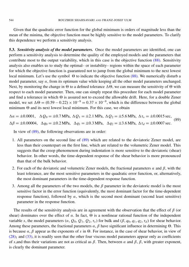
5.3. Sensitivity analysis of the model parameters. Once the model parameters are identified, one canperform a sensitivity analysis to determine the quality of the employed models and the parameters thatcontribute most to the output variability, which in this case is the objective function (88). Sensitivityanalysis also enables us to study the optimal– or instability– regions within the space of each parameterfor which the objective function is guaranteed not to jump from the global minimum to the next lowestlocal minimum. Let’s use the symbol 2 to indicate the objective function (88). We numerically disturb amodel parameter, say α, from its optimum value while keeping all the other model parameters unchanged.Next, by monitoring the change in 2 to a defined tolerance 12, we can measure the sensitivity of 2 withrespect to each model parameter. Then, one can simply repeat this procedure for each model parameterand find a tolerance in which 2 is assured not to exceed the allowable drift. Here, for a double Zenermodel, we set 12 = (0.59− 0.22)× 10−9

= 0.37× 10−9, which is the difference between the globalminimum 2 and its next lowest local minimum. For this case, we obtain

1α =±0.0001, 1Q0 =±0.7 MPa, 1Q1 =±2.1 MPa, 1Q2 =±5.6 MPa, 1τv =±0.0015 sec,

1β =±0.00004, 1q0 =±0.2 MPa, 1q1 =±0.3 MPa, 1q2 =±3.6 MPa, 1τd =±0.0007 sec.(89)

In view of (89), the following observations are in order:

1. All parameters on the second line of (89) which are related to the deviatoric Zener model, areless than their counterpart on the first line, which are related to the volumetric Zener model. Thissuggests that the creep phenomenon during indentation is more sensitive to the deviatoric (shear)behavior. In other words, the time-dependent response of the shear behavior is more pronouncedthan that of the bulk behavior.

2. For each of the deviatoric and volumetric Zener models, the fractional parameters α and β, with theleast tolerance, are the most sensitive parameters in the quadratic error function, or, alternatively,the most dominant parameters in the time-dependent response function.

3. Among all the parameters of the two models, the β parameter in the deviatoric model is the mostsensitive factor in the error function (equivalently, the most dominant factor for the time-dependentresponse function), followed by α, which is the second most dominant (second least sensitive)parameter in the response function.

The results of the sensitivity analysis are in agreement with the observation that the effect of β (orshear) dominates over the effect of α. In fact, 2 is a nonlinear rational function of the independentvariable s, the model parameters (α, Q0, Q1, Q2, τv) for bulk and (β, q0, q1, q2, τd) for shear behavior.Among these parameters, the fractional parameters α, β have significant influence in determining 2. Thisis because α, β appear as the exponents of s in 2. For instance, in the case of shear behavior, in view of(28)1 and (33), it is readily seen that the other four viscous model parameters appear only as coefficientsof s,and thus their variations are not as critical as β. Then, between α and β, β, with greater exponent,is clearly the dominant parameter.

INDENTATION ANALYSIS OF FRACTIONAL VISCOELASTIC SOLIDS 545

6. Conclusions

The fractional viscoelastic model offers new possibilities for the characterization of materials whose time-dependent response may be poorly captured by classical integer-type viscoelastic models. The analysisand method developed in this paper aims at determining the fractional properties from indentation anal-ysis. The following conclusions can be drawn:

(i) The derived constitutive differential equations governing the indentation response show that thedifferential order of the constitutive differential equations of the indentation response is higher thanthe one governing the material level. This difference in differential order between the material scaleand indentation scale holds for both fractional and integer-type viscoelastic models, the latter beingrecognized as a subset of the more general fractional modeling framework. The found difference is morepronounced for the viscoelastic shear response than for the viscoelastic bulk response. This is explicitlyshown with higher order derivatives in β than in α for fractional viscoelastic materials. This observationis in agreement with the sensitivity analysis performed on the error function, and it translates into thewell-known fact that an indentation test is rather a shear test than a hydrostatic test.

(ii) The general constitutive differential equations are readily employed to derive indentation creep andrelaxation functions, which, analogously to uniaxial creep compliance and relaxation functions, can beused in fractional indentation analysis for any monotonically increasing force- or depth-load historiesapplied in indentation testing. On this basis, explicit solutions for specific fractional creep models can bederived, as illustrated for the double Zener, double Maxwell, and deviatoric Maxwell and Zener models.

(iii) In order to translate time-dependent indentation data into fractional material model properties, wesuggest fitting the experimental response to the model response in the Laplace domain. This reducesthe mathematical complexity of obtaining properties from indentation data without compromising theaccuracy of the fit in the time domain. Our optimization method has two important features: the optimummodel parameters do not depend on the initial parameter guesses; and in our curve-fitting on the complexplane, all functions are treated as real functions by making use of the Identity Theorem.

Appendix

The fractional expression D(s) can be converted into a polynomial of integer order by

D(s)=∑

j

b j s j/m=

∑j

b j u j= X (u), (90)

where u j= s j/m , and m > 0 is the smallest common denominator of the fractional parameters α and β.

Some of the coefficients b j are clearly zero, while any non-zero b j corresponds to the coefficient of sin D(s) whose exponent becomes equal to j/m. The inverse transform of a function, f (s), exists andis real, continuous, and causal when (i) f (s) is analytic for Re(s) > 0, (ii) f (s) is real for s real andpositive, (iii) f (s) is of order s−γ , where γ > 1, for |s| large in the right half s plane [Churchill 1958].One can simply show that L(s) in (56) satisfies all three conditions. By definition, the inverse Laplace

546 ROUZBEH SHAHSAVARI AND FRANZ-JOSEF ULM

γ

1

2

6

3

5

4

Figure 9. Integration contour on the complex s-plane for the calculation of (91).

transform of (56) is then

L(t)=1

2π i

∫ γ+i∞

γ−i∞est DF (s)

2s Dh(s)ds. (91)

One can evaluate this line integral by extending it into a closed contour integration, as in Figure 9.Recall that the residue theorem states that the integral along any closed contour, divided by 2π i , is equalto the sum of the residues of poles of the integrand within that contour. The contour in Figure 9, isdivided into six segments with arrows which indicate the direction of integration. (Segments 3, 4, 5 areneeded since the branch cut of s1/m lies along the negative real axis.) We thus can write

12π i

∫C1

est DF (s)

2s Dh(s)ds+

12π i

6∑k=2

∫Ck

est DF (s)

2s Dh(s)ds =

∑j

b j , (92)

where b j are the residues. Equation (91) is the first term in (92) when its limits are extended to infinityin the negative and positive imaginary directions of the s plane. The radii of the segments 2 and 6are increased infinitely to ensure the continuity of the closed contour. Similarly, segments 3 and 5 arestretched to infinity on the negative real axis. When the radius approaches infinity, it can be shown thatthe integrals along the contours 2 and 6 are zero. By using the following lemma [MacRobert 1962] onecan obtain the contour integral along the segment 4,

Lemma. If lim(s − a) f (s) = k as s→ a, where k is a constant, then lim∫

f (s)ds = i(θ2 − θ1)k, theintegral being taken for s→ a and r→ 0 around an arc from θ1 to θ2 of the circle |s− a| = r .

It follows that since (θ2− θ1)= 0, ∫4

est DF (s)

2s Dh(s)ds = 0. (93)

One can also show that∫3

est DF (s)

2s Dh(s)ds+

∫5

est DF (s)

2s Dh(s)ds =−2i Im

∫∞

0e−r t

DF (re−iπ )

2s Dh(re−iπ )dr. (94)

INDENTATION ANALYSIS OF FRACTIONAL VISCOELASTIC SOLIDS 547

Finally, using the conventional technique, the residues are calculated as

b j = lims→λm

j

(s− λmj )

DF (s)

2s Dh(s)est . (95)

Here, λ j refers to the j -th root of the integer polynomial X (u). In view of equations (90) and (56), theroots of X (u) correspond to the poles of L(t). Lastly, by substituting (93), (94), and (95) into (92), onecan find the general solution in the time domain. For specific solutions, we need to consider differentmodels. For a double Zener models, since all the c and l coefficients in (42) are nonzero, s = 0 in (56) is asimple pole, and because its exponent is one and an integer number, this pole is on the s-plane. Thus, itsresidue via (95) is simply the first term in (59). Other poles of (56) λi (those that make Dh(s)= 0) werefound in the s1/m plane. Since the Laplace transform is performed in the s-plane, the poles λi should betransformed into λm

i to be on the s-plane. However, that transformation maps some of the original polesonto Riemann surfaces out of the closed contour of integration in the s−plane. Thus, according to theresidue theorem, the residues of such poles do not contribute to the solution. Hence, the summation overthe index j in (59) (and through all equations in this paper) pertains only to those poles that remain inthe closed contour’s plane after the transformation. This indicates that, for a linear physical system, λm

imust have a negative real part in order for the system to be stable.

For double Maxwell models, c0 = l0 = l1 = l2 = 0, and (56) simplifies to

L(s)=DF (s)

2s Dh(s)=

c1sα + c2sβ + c3sα+β + c4sα+2β+ c5s2β

2s(l3sα+β + l4sα+2β + l5s2β). (96)

In the case of α ≤ β, after cancelling out sα, (96) yields

L(s)=c1+ c2sβ−α + c3sβ + c4s2β

+ c5s2β−α

2s1+β(l3+ l4sβ + l5sβ−α). (97)

Clearly, s = 0 in (97) is not a simple pole, rather, it is a pole of fractional order 1 + β. Considerthis fractional number to be k/m, where k and m are two integer numbers. By using the followingtransformation:

s1+β= (s1/m)k = uk, (98)

one can convert (97) into quotient of two polynomials as

L(u)=c1+ c2um(β−α)

+ c3umβ+ c4u2mβ

+ c5um(2β−α)

2uk(l3+ l4umβ + l5um(β−α)). (99)

Now, u = 0 in (99) is a multiple pole of order k. In order to find its residue, we use the fact that theresidue of a function f (s)= Q(s)/(s− a)n+1 at a multiple pole a of order n+ 1 is given by

F(s, t)=1n!∂n

∂ns[Q(s)est

]s=a.

(see [Churchill 1958], for example). Applying this to (99) leads to (61)1. Similarly, in the case of α > β,after cancelling out sβ , one can find (61)2. The residue theorem in conjunction with fractional-orderderivatives has been used in [Bagley and Torvik 1983] and [Ostoja-Starzewski and Shahsavari 2008] ina slightly different way.

548 ROUZBEH SHAHSAVARI AND FRANZ-JOSEF ULM

References

[Abate and Valkó 2004] J. Abate and P. P. Valkó, “Multi-precision Laplace transform inversion”, Int. J. Numer. Methods Eng.60 (2004), 979–993.

[Arkhincheev 1993] V. E. Arkhincheev, “Anomalous diffusion in inhomogeneous media: some exact results”, Model. Meas.Control A 26:2 (1993), 11–29.

[Bagley and Torvik 1983] R. L. Bagley and P. J. Torvik, “A theoretical basis for the application of fractional calculus toviscoelasticity”, J. Rheol. 27:3 (1983), 201–210.

[Baker et al. 1996] W. P. Baker, L. B. Eldred, and A. Palazotto, “Viscoelastic material response with a fractional-derivativeconstitutive model”, AIAA J. 34:3 (1996), 596–600.

[Bland 1960] D. R. Bland, The theory of linear viscoelasticity, International Series of Monographs on Pure and Applied Math-ematics 10, Pergamon, New York, 1960.

[Borodich and Galanov 2008] F. M. Borodich and B. A. Galanov, “Non-direct estimations of adhesive and elastic properties ofmaterials by depth-sensing indentation”, Proc. R. Soc. Lond. A 464:2098 (2008), 2759–2776.

[Borodich and Keer 2004] F. M. Borodich and L. M. Keer, “Contact problems and depth-sensing nanoindentation for friction-less and frictional boundary conditions”, Int. J. Solids Struct. 41:9–10 (2004), 2479–2499.

[Boussinesq 1885] J. Boussinesq, Applications des potentiels à l’étude de l’équilibre et du mouvement des solides élastiques,Gauthier-Villars, Paris, 1885.

[Brinell 1901] J. A. Brinell, “Mémoire sur les épreuves à bille en acier”, pp. 83–94 in Communications presentés devant leCongrés International des Méthodes d’Essai des Matériaux de Construction (Paris, 1900), vol. 2, edited by P. Debray and L.Baclé, Dunod, Paris, 1901.

[Bulychev 1999] S. I. Bulychev, “Relation between the reduced and unreduced hardness in nanomicroindentation tests”, Tech.Phys. 44:7 (1999), 775–781.

[Caputo 1967] M. Caputo, “Linear models of dissipation whose Q is almost frequency independent, Part II”, Geophys. J. Int.13:5 (1967), 529–539.

[Caputo 1969] M. Caputo, Elasticità e dissipazione, Zanichelli, Bologna, 1969.

[Cariou et al. 2008] S. Cariou, F.-J. Ulm, and L. Dormieux, “Hardness-packing density scaling relations for cohesive-frictionalporous materials”, J. Mech. Phys. Solids 56:3 (2008), 924–952.

[Carrier et al. 1966] G. F. Carrier, M. Krook, and C. E. Pearson, Functions of a complex variable: theory and technique,McGraw-Hill, New York, 1966.

[Cheng and Cheng 2004] Y.-T. Cheng and C.-M. Cheng, “Scaling, dimensional analysis, and indentation measurements”, Mater.Sci. Eng. R 44:4–5 (2004), 91–149.

[Cheng et al. 2000] L. Cheng, H. Xia, W. Yu, L. E. Scriven, and W. W. Gerberich, “Flat-punch indentation of viscoelasticmaterials”, J. Polym. Sci. B Polym. Phys. 38:1 (2000), 10–22.

[Cheng et al. 2005] L. Cheng, X. Xia, L. E. Scriven, and W. W. Gerberich, “Spherical-tip indentation of viscoelastic material”,Mech. Mater. 37:1 (2005), 213–226.

[Christensen 1971] R. M. Christensen, Theory of viscoelasticity: an introduction, Academic Press, New York, 1971.

[Churchill 1958] R. V. Churchill, Operational mathematics, 2nd ed., McGraw-Hill, New York, 1958.

[Coleman and Li 1994] T. F. Coleman and Y. Li, “On the convergence of interior-reflective Newton methods for nonlinearminimization subject to bounds”, Math. Program. 67:2, Ser. A (1994), 189–224.

[Coleman and Li 1996] T. F. Coleman and Y. Li, “An interior trust region approach for nonlinear minimization subject tobounds”, SIAM J. Optim. 6:2 (1996), 418–445.

[Constantinides 2006] G. Constantinides, Invariant mechanical properties of Calcium-Silicate-Hydrates (C-S-H) in cement-based materials: instrumented nanoindentation and micromechanical modeling, Ph.D. thesis, Department of Civil and Envi-ronmental Engineering, Massachusetts Institute of Technology, 2006.

[Doerner and Nix 1986] M. F. Doerner and W. D. Nix, “A method for interpreting the data from depth-sensing indentationinstruments”, J. Mater. Res. 1:4 (1986), 601–609.

INDENTATION ANALYSIS OF FRACTIONAL VISCOELASTIC SOLIDS 549

[Engheta 1996] N. Engheta, “On fractional calculus and fractional multipoles in electromagnetism”, IEEE Trans. Antenn.Propag. 44:4 (1996), 554–566.

[Flügge 1967] W. Flügge, Viscoelasticity, Blaisdell, Waltham, MA, 1967.

[Galanov 1982] B. A. Galanov, “An approximate method for the solution of some two-body contact problems with creep in thecase of an unknown contact area”, Sov. Appl. Mech. 18:8 (1982), 711–718.

[Galin 1961] L. A. Galin, Contact problems in the theory of elasticity, edited by I. N. Sneddon, North Carolina State College,Raleigh, NC, 1961.

[Ganneau et al. 2006] F. P. Ganneau, G. Constantinides, and F.-J. Ulm, “Dual-indentation technique for the assessment ofstrength properties of cohesive-frictional materials”, Int. J. Solids Struct. 43:6 (2006), 1727–1745.

[Gao and Ogden 2003] D. Y. Gao and R. W. Ogden (editors), Advances in mechanics and mathematics, Volume II, Advancesin Mechanics and Mathematics 4, Kluwer Academic, Boston, 2003.

[Glöckle and Nonnenmacher 1991] W. G. Glöckle and T. F. Nonnenmacher, “Fractional integral operators and Fox functionsin the theory of viscoelasticity”, Macromolecules 24:24 (1991), 6426–6434.

[Hertz 1882] H. Hertz, “Über die Bierührung fester elastischer Körper”, J. Reine Angew. Math. 92 (1882), 156–171. Translatedin Miscellaneous papers by H. Hertz, Jones and Schott (Eds.), Macmillan, London, 1896.

[Kilbas et al. 2006] A. A. Kilbas, H. M. Srivastava, and J. J. Trujillo, Theory and applications of fractional differential equa-tions, North-Holland Mathematics Studies 204, Elsevier, Amsterdam, 2006.

[Lee 1955] E. H. Lee, “Stress analysis in visco-elastic bodies”, Quart. Appl. Math. 13 (1955), 183–190.

[Lee and Radok 1960] E. H. Lee and J. R. M. Radok, “The contact problem for viscoelastic bodies”, J. Appl. Mech. (ASME)27 (1960), 438–444.

[Love 1939] A. E. H. Love, “Boussinesq’s problem for a rigid cone”, Quart. J. Math. Oxford Ser. (2) 10:1 (1939), 161–175.

[MacRobert 1962] T. M. MacRobert, Functions of a complex variable, 5th ed., Macmillan, London, 1962.

[Marsden and Hoffman 1999] J. E. Marsden and M. J. Hoffman, Basic complex analysis, 3rd ed., W. H. Freeman, New York,1999.

[Micromaterials 2002] Micromaterials nanotest user manual, Micromaterials, Wrexhham, 2002.

[Oliver and Pharr 1992] W. C. Oliver and G. M. Pharr, “An improved technique for determining hardness and elastic modulususing load and displacement sensing indentation experiments”, J. Mater. Res. 7:6 (1992), 1564–1583.

[Ostoja-Starzewski and Shahsavari 2008] M. Ostoja-Starzewski and H. Shahsavari, “Response of a helix made of a fractionalviscoelastic material”, J. Appl. Mech. (ASME) 75:1 (2008), 011012.

[Oyen 2005] M. L. Oyen, “Spherical indentation creep following ramp loading”, J. Mater. Res. 20:8 (2005), 2094–2100.

[Oyen 2006] M. L. Oyen, “Analytical techniques for indentation of viscoelastic materials”, Philos. Mag. 86:33–35 (2006),5625–5641.

[Podlubny 1999] I. Podlubny, Fractional differential equations, Mathematics in Science and Engineering 198, Academic Press,San Diego, CA, 1999.

[Rabotnov 1980] J. N. Rabotnov, Elements of hereditary solid mechanics, Mir, Moscow, 1980.

[Radok 1957] J. R. M. Radok, “Visco-elastic stress analysis”, Quart. Appl. Math. 15 (1957), 198–202.

[Ross 1977] B. Ross, “Fractional calculus”, Math. Mag. 50:3 (1977), 115–122. An historical apologia for the development ofa calculus using differentiation and antidifferentiation of non-integral orders.

[Rossikhin and Shitikova 2004] Y. A. Rossikhin and M. V. Shitikova, “Analysis of the viscoelastic rod dynamics via modelsinvolving fractional derivatives or operators of two different orders”, Shock Vib. Digest 36:1 (2004), 3–26.

[Sakai 1999] M. Sakai, “The Meyer hardness: a measure for plasticity?”, J. Mater. Res. 14:9 (1999), 3630–3639.

[Schiessel and Blumen 1993] H. Schiessel and A. Blumen, “Hierarchical analogues to fractional relaxation equations”, J. Phys.A Math. Gen. 26:19 (1993), 5057–5069.

[Schiessel et al. 1995] H. Schiessel, R. Metzler, A. Blumen, and T. F. Nonnenmacher, “Generalized viscoelastic models: theirfractional equations with solutions”, J. Phys. A Math. Gen. 28:23 (1995), 6567–6584.

550 ROUZBEH SHAHSAVARI AND FRANZ-JOSEF ULM

[Shahsavari and Ostoja-Starzewski 2005] H. Shahsavari and M. Ostoja-Starzewski, “On elastic and viscoelastic helices”, Philos.Mag. 85:33–35 (2005), 4213–4230.

[Shimizu et al. 1999] S. Shimizu, T. Yanagimoto, and M. Sakai, “Pyramidal indentation-depth curve of viscoelastic materials”,J. Mater. Res. 14:10 (1999), 4075–4086.

[Sneddon 1965] I. N. Sneddon, “The relation between load and penetration in the axisymmetric Boussinesq problem for apunch of arbitrary profile”, Int. J. Eng. Sci. 3:1 (1965), 47–57.

[Tabor 1951] D. Tabor, Hardness of metals, Clarendon, Oxford, 1951.

[Tschoegl et al. 2002] N. W. Tschoegl, W. G. Knauss, and I. Emri, “Poisson’s ratio in linear viscoelasticity: a critical review”,Mech. Time-Depend. Mat. 6:1 (2002), 3–51.

[Vandamme and Ulm 2006] M. Vandamme and F.-J. Ulm, “Viscoelastic solutions for conical indentation”, Int. J. Solids Struct.43:10 (2006), 3142–3165.

[Vandamme and Ulm 2007] M. Vandamme and F.-J. Ulm, “Indenter-shape independent viscoelastic solutions for indentationcreep and relaxation testing”, C. R. Mécanique (2007). Submitted.

Received 12 Oct 2008. Revised 22 Dec 2008. Accepted 4 Feb 2009.

ROUZBEH SHAHSAVARI: shahs@mit.eduDepartment of Civil and Environmental Engineering, Massachusetts Institute of Technology, 77 Massachusetts Avenue,Cambridge, MA 02139-4307, United States

FRANZ-JOSEF ULM: ulm@mit.eduDepartment of Civil and Environmental Engineering, Massachusetts Institute of Technology, 77 Massachusetts Avenue,Cambridge, MA 02139-4307, United States