Journal of Hydrology, 111 (1989) 377-390 377 Elsevier Science Publishers B.V., Amsterdam - - Printed in The Netherlands

[41

UNIT H Y D R O G R A P H STABILITY A N D LINEAR A L G E B R A

JAMES C.I. DOOGE and MICHAEL BRUEN

Department of Engineering Hydrology, University College, Galway (Ireland)

(Received November 5, 1987; accepted after revision September 9, 1988)

ABSTRACT

Dooge, J.C.I. and Bruen, M., 1989. Unit hydrograph stability and linear algebra. J. Hydrol., 111: 377-390.

The paper explores the feasibility of using concepts from linear algebra such as the condition number as a basis for studying the conditions under which data error causes unacceptable insta- bilities in derived unit hydrographs. The condition number, which provides an upper bound for the amplification of error is shown to depend on the shape of the input time-series and the method of deriving the unit hydrograph. A number of methods (forward substitution, Collins' method, least squares and smoothed least squares) are compared for the highly simplified case of a two-ordinate unit hydrograph for which a closed form solution can be obtained in each case.

INTRODUCTION

Hydrologists have long been aware of the difficulties of deriving a stable unit hydrograph from error-prone data and have developed a large number of different methods to cope with the problem. The early trial-and-error approaches were succeeded by less subjective methods based on linear algebra, optimisation or linear transforms. Systematic comparison of these methods by numerical experimentation was pioneered by Laurenson and O'Donnell (1969) and was extended by Garvey (1972) and Bruen (1977). The results of these studies have been summarised by Dooge (1979). While a comparison based on numerical experiments gives useful results, one based on analytical methods should be of greater value. This paper is a preliminary exploration of how such an analytical approach might be made. The required mathematical formulation is introduced and illustrated with the simple case of only two ordinates in the unit hydrograph for which an explicit, closed-form solution is possible. The application to more complex data, both synthetic and actual, will be described in a second paper.

BASIC EQUATIONS

For the case of a linear, time-invariant, lumped system, the convolution equation can be written in discrete form as (Dooge, 1973):

0022-1694/89/$03.50 © 1989 Elsevier Science Publishers B.V.

378

_L Ys = ~ h i x s + l - j s = 1 , 2 , 3 . . . . . p (1)

j 1

where: x~ is the volume of input during the j th time interval; Yi is the output, sampled at the end of the j th time interval; h i is the j th sampled value of the pulse response; and p is the number of sampled output values.

This equation applies to isolated events, but can also be used to relate the autocorrelation of the input series with the crosscorrelation of the input and output series (Eagleson et al, 1966). It gives p simultaneous linear algebraic equations, which can, for convenience, be written in matrix form as:

X h = y (2)

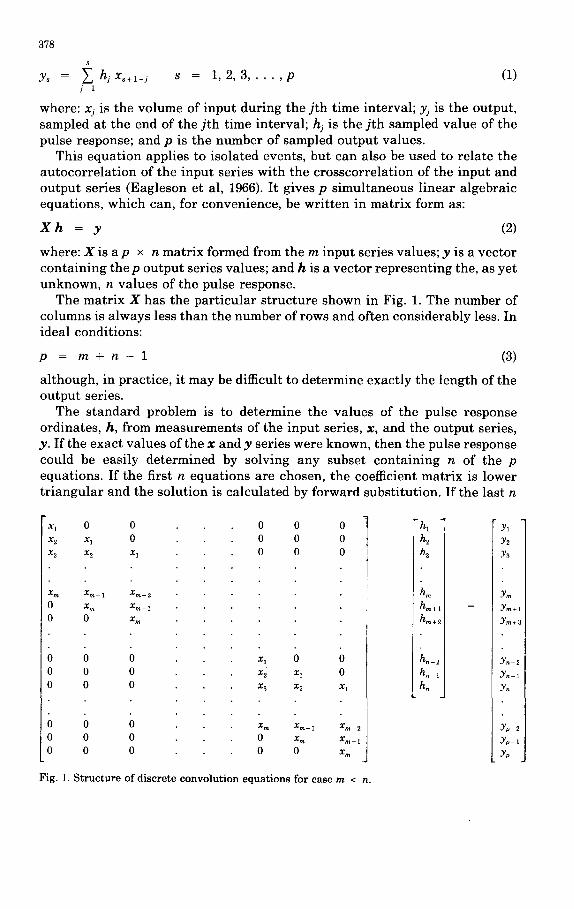
where: X is a p × n matrix formed from the m input series values; y is a vector conta in ing t h e p output series values; and h is a vector represent ing the, as yet unknown, n values of the pulse response.

The matrix X has the particular structure shown in Fig. 1. The number of co lumns is a lways less than the number of rows and often considerably less. In ideal condit ions:

p = m + n - 1 (3)

although, in practice, it may be difficult to determine exactly the length of the output series.

The standard problem is to determine the values of the pulse response ordinates, h, from measurements of the input series, x, and the output series, y. If the exact values of the x and y series were known, then the pulse response could be easily determined by solving any subset containing n of the p equations. If the first n equations are chosen, the coefficient matrix is lower tr iangular and the solution is calculated by forward substitution. If the last n

i 0 0 x 2 x 1 0 3 X2 X l

Xm Xm 1 Xm - 2

0 X m X m - 1

0 0 x,.

0 0 0 0 0 0 0 0 0

0 0 0 0 0 0 0 0 0

0 0 0 0 0 0 0 0 0

xl 0 x~ xl 0 X3 X2 X 1

Xm Xm - 1 Xm 2

0 X m Xm - 1

0 0 x,.

Fig. 1. S t ruc tu re of discrete convolut ion equat ions for case m < n.

h 1

h2 ha

ho hm÷ ]

hm+,

h. j

21

Y2 Y3

Y~ Y m + l

Ym~ 3

Y n - 2

Y n - 1

Y~

Yp-2 1 Yp-l[ y , j

379

equations are chosen, the coefficient matrix is upper t r iangular and the solution is calculated by backward substitution.

METHODS OF UNIT HYDROGRAPH ESTIMATION

Hydrologists soon encountered practical difficulties in deriving realistic unit hydrographs using the basic equations and developed a number of useful variat ions of the method. Collins (1939) suggested a variat ion of the trial and error approach in which the most recent estimate of the unit hydrograph is applied to all rainfall values except the maximum one. The resulting calculated runoff is subtracted from the actual runoff to give the runoff due to the maximum ordinate alone and this is used to update the previous estimate of the unit hydrograph. Collins' method is equivalent to selecting and solving the n equations which contain the maximum rainfall value and neglecting the other equations. Barnes (1959) suggested using both forward and backward sub- st i tution and the adjustment of the input values until the estimates from each method are close.

The least-squares methods allow all p equations to be used simultaneously in determining a solution which is optimal in the ~'minimum squared deviations" sense. The unit hydrograph is the solution of:

(XTX) h - Xry (4)

Kuchment (1967) applied the regularisat ion technique developed by Tikhonov (1965) to derive a smoothed least squares estimate of the unit hydrograph. This extension of the least squares method can be implemented with a minimal amount of extra computation, Bruen and Dooge (1984). The unit hydrograph for this method is the solution of:

(Xr X + k I ) h - X'r y (5)

O'Donnell (1960) applied linear transform methods to unit hydrograph estimation and used the simple linkage equation between the harmonic transforms of the input, output and unit hydrograph. Dooge (1965) used Laguerre transforms and Dooge and Garvey (1978) used Meixner transforms, both of which have more complex linkage equations, to estimate unit hydrographs.

EFFECTS OF DATA ERRORS

Almost all the methods used in practice to estimate unit hydrographs reduce the problem to the solution of a square set of simultaneous equations:

A /~ = b (6)

where the square matrix A and the right-hand side vector b depend both on the data and the estimation method. For the direct methods - - forward and backward substi tution and Collins' method - - the matrix A contains a selection of rows from the convolution matrix X. The right-hand side vector b

380

contains the corresponding values from the output series y. For the ordinary least-squares method, eqn. (4), the matrix A is the set of "normal" coefficients XTX and the vector b is the corresponding right-hand side XWy. For the smoothed least-squares method, eqn. (5), a constant k is added to the diagonal of the matrix x r x . In all these methods, the unit hydrograph estimate is the solution of eqn. (6), which can be writ ten formally as:

ft = A- lb (7)

The presence of the inverse of a matrix in the formal solution inevitably raises the question of the numerical stability of an estimate based on data which is subject to measurement errors.

Since the convolut ion of the input series with the catchment response is a smoothing operation, the reverse process, a deconvolution to estimate the unit hydrograph, amplifies any data or modelling errors. This amplification often leads to unstable and physically unrealistic unit hydrograph estimates. Standard relationships from linear algebra can be used to analyse the ampli- fication. A unique, real-valued, function of the matrix, A, called its condition number, is found to provide an upper bound on the error amplification. The derivation and use of the condition number is explained in the Appendix. The remainder of this paper i l lustrates the behaviour of the condition number for a very simple case, for which a closed form result can be obtained. A fur ther paper will deal with a more practical application of these results.

CONDITION NUMBER FOR A SIMPLE CASE

In the very simple case, where only two unit hydrograph ordinates are estimated, a closed-form expression can be derived for the condition number, given by eqn. (A32) in the Appendix, because only two eigenvalues are involved and these are the roots of a quadrat ic equation.

In the case of two unknown unit hydrograph ordinates, the matrix, A, has only two rows and two columns. Hence ATA can be writ ten as:

AT A = (Cll c121 (8)

\C21 C22/

The eigenvalues, ~, of the matrix are the roots of the equation:

(cn - ~)(c22 - ~) - c1~c21 = 0 (9)

The condition number, which is defined and derived in the Appendix, is given by eqn. (A32) as:

/~max 1/2 K(A) = ~ (10)

and, in this case, is:

K(A) = c + ~ - 1 (11)

381

where:

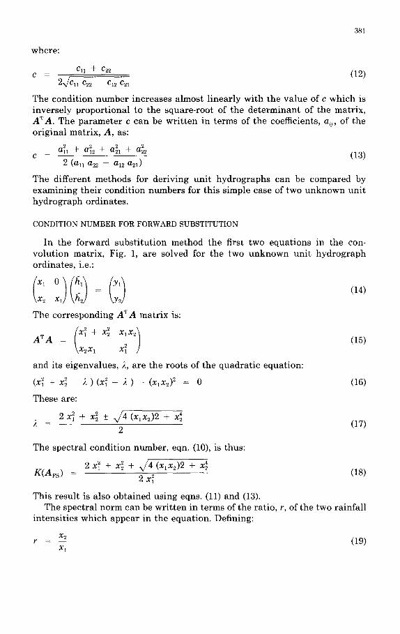
C = Cll -}- c22 (12) 2X/Cll C22 -- C12 C21

The condi t ion number increases a lmost l inear ly wi th the va lue of c which is inverse ly p ropor t iona l to the square- root of the d e t e rm in an t of the matr ix , A T A . The pa rame te r c can be wr i t t en in terms of the coefficients, aij, of the or iginal matr ix , A, as:

a~l + a22 + a21 + a222 c = (13)

2 (a,, a22 -- a12 a21 )

The dif ferent methods for der iv ing uni t hydrographs can be compared by examin ing the i r condi t ion numbers for this simple case of two u n k n o w n uni t hyd rog raph ordinates .

CONDITION N U M B E R FOR FORWARD SUBSTITUTION

In the forward subs t i tu t ion me thod the first two equat ions in the con- vo lu t ion matr ix , Fig. 1, are solved for the two u n k n o w n uni t hyd rog raph ordinates , i.e.:

The cor responding A T A matr ix is:

+ x,x I A T A = (15)

~x2xl x~ /

and its e igenvalues , 2, are the roots of the quadra t i c equat ion:

(x~ + x~ - 2 ) (x 2 - 2 ) - (x , x2) 2 = 0 (16)

These are:

2 x/4 (x, x2)2 + x 4 2 xl + x~ _+ 2 = (17)

2

The spectra l condi t ion number , eqn. (10), is thus:

2 x~ + x~ + , / 4 (XlX2)2 + x 4 K(Ars) = 2 x~ (18)

This resu l t is also ob ta ined using eqns. (11) and (13). The spect ra l norm can be wr i t t en in terms of the rat io, r, of the two rainfal l

in tens i t ies which appear in the equat ion. Defining:

X2 r - (19)

Xl

382

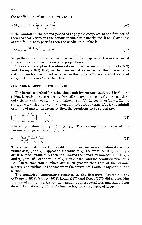
the condition number can be writ ten as:

r2 ~ r4 K(AFs ) = 1 + ~ + r2+--4 (20)

If the rainfall in the second period is negligible compared to the first period then r is nearly zero and the condition number is nearly one. If equal amounts of rain fall in both periods then the condition number is:

K(A~s) _ 3 + ~ _ 2.62 (21) 2

When the rainfall in the first period is negligible compared to the second period the condition number increases in proportion to r 2.

These results explain the observations of Laurenson and O'Donnell (1969) and Garvey (1972) that, in their numerical experiments, the forward sub- st i tution method performed better when the higher effective rainfall occurred early in the storm ra ther than later.

CONDITION NUMBER FOR COLLINS METHOD

The i terat ive method for estimating a unit hydrograph, suggested by Collins (1939), is equivalent to selecting from all the available convolution equations only those which contain the maximum rainfall intensity ordinate. In the simple case, with only two unknown unit hydrograph terms, ifxk is the rainfall ordinate of maximum intensity then the equations to be solved are:

Xk + 1 Xk h2 Yk +1

where, by definition, xh 1 ~< xk /> xk+l. The corresponding value of the parameter, c, given by eqn. (12), is:

X 2 k 1 + 2x~ + x~+ 1 c = (23)

2(x~ - xk lx~+1)

This value, and hence the condition number, increases indefinitely as the values of xk_l and Xk÷l approach the value of xk. For instance, if xk_l and xk÷~ are 90% of the value of xk then c is 9.53 and the condition number is 19. If x~_ 1 and xk÷l are 99% of the value of xk then c is 99.5 and the condition number is 199. These condition numbers are much greater than that of the forward substi tution method, in the case when the first rainfall value is higher than the second.

The numerical experiments reported in the literature, Laurenson and O'Donnell (1969), Garvey (1972), Bruen (1977) and Dooge (1979) did not consider the case of an input series with x~ ~ and xk÷l almost equal to xk and thus did not detect the instability of the Collins method for these types of input.

383

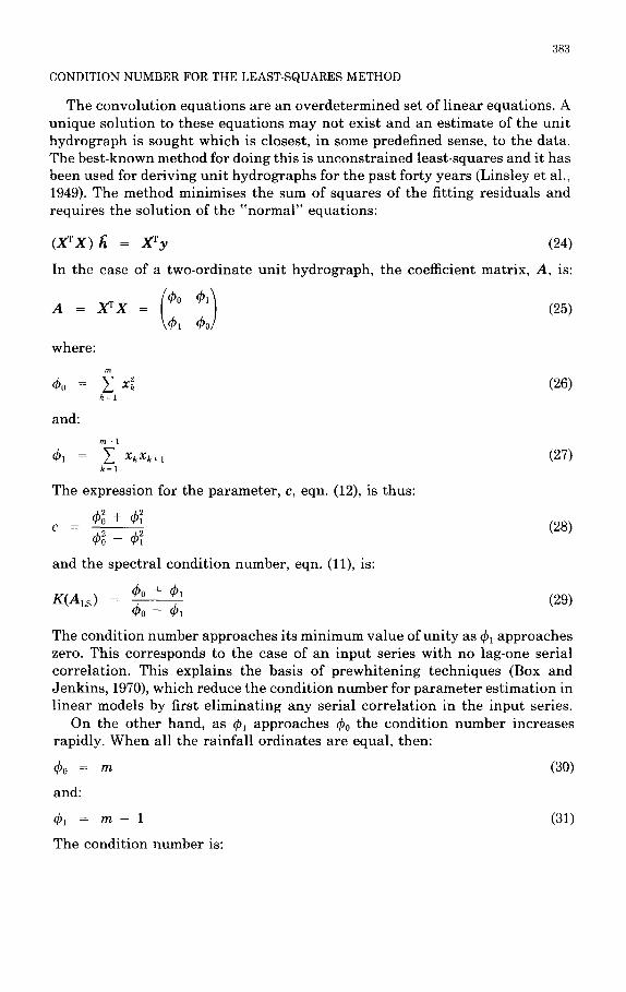
CONDITION NUMBER FOR THE LEAST-SQUARES METHOD

The convolution equations are an overdetermined set of l inear equations. A unique solution to these equations may not exist and an estimate of the unit hydrograph is sought which is closest, in some predefined sense, to the data. The best-known method for doing this is unconstrained least-squares and it has been used for deriving unit hydrographs for the past forty years (Linsley et al., 1949). The method minimises the sum of squares of the fitting residuals and requires the solution of the ~'normal" equations:

(XrX) ~ = Xry (24)

In the case of a two-ordinate unit hydrograph, the coefficient matrix, A, is:

A = X r x

where:

4 0 = k - 1

and:

41 =

(26)

m - 1

XkXk÷ l (27) k = l

The expression for the parameter, c, eqn. (12), is thus:

c - (28) 4 0 -

and the spectral condition number, eqn. (11), is:

40 + 41 K(ALs) - (29) 4 0 -

The condition number approaches its minimum value of unity as 41 approaches zero. This corresponds to the case of an input series with no lag-one serial correlation. This explains the basis of prewhitening techniques (Box and Jenkins, 1970), which reduce the condition number for parameter estimation in linear models by first eliminating any serial correlat ion in the input series.

On the other hand, as 4~ approaches 40 the condition number increases rapidly. When all the rainfall ordinates are equal, then:

40 = m (30)

and:

4~ = m - 1 (31)

The condition number is:

384

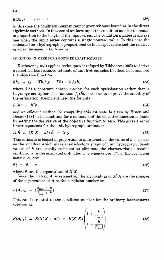
K(ALs) = 2 m - 1 (32)

In this case the condition number cannot grow without bound as in the direct algebraic methods. In the case of uniform input the condition number increases in proportion to the length of the input series. The condition number is always one when the input series contains a single nonzero value. In this case the estimated unit hydrograph is proportional to the output series and the relative error is the same in both series.

CONDITION NUMBER FOR SMOOTHED LEAST-SQUARES

Kuchment (1967) applied techniques developed by Tikhonov (1965) to derive a smoothed least-squares estimate of unit hydrographs. In effect, he minimised the objective function:

f(/~) = (3, - X h ) W ( y - - X~$) + k fa(h) (33)

where k is a constant, chosen a-priori for each optimisation rather than a Lagrange multiplier. The function, fl (h), is chosen to improve the stability of the estimation. Kuchment used the formula:

fl (h) = ~T~ (34)

and an efficient method for computing this estimate is given by Bruen and Dooge (1984). The condition for a minimum of the objective function is found by setting the derivative of the objective function to zero. This gives a set of linear equations for the unit hydrograph ordinates:

A h =_ ( x r x + k I ) h = X r y (35)

This estimate is biased in proportion to k. In practice, the value of k is chosen as the smallest which gives a satisfactory shape of unit hydrograph. Small values of k are usually sufficient to eliminate the characteristic unstable oscillations in the estimated ordinates. The eigenvalues, 0", of the coefficient matrix, A, are:

0 7 : 0j + k (36)

where 0j are the eigenvalues of XTx. Since the matrix, A, is symmetric, the eigenvalues of A T A are the squares

of the eigenvalues of A so the condition number is:

Oma x + k K(Asas) = [ 0rain + k I (37)

This can be related to the condition number for the ordinary least-squares solution as:

K(AsLs) = K ( X T X + k I ) = K ( X T X ) - - (38)

385

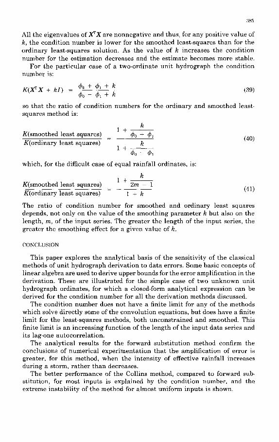
All the eigenvalues of X r x are nonnegative and thus, for any positive value of k, the condition number is lower for the smoothed least-squares than for the ordinary least-squares solution. As the value of k increases the condition number for the estimation decreases and the estimate becomes more stable.

For the particular case of a two-ordinate unit hydrograph the condition number is:

K ( x r x + k I ) = ~)o + ~)1 + k (39) ¢0 - ~1 + k

so that the ratio of condition numbers for the ordinary and smoothed least- squares method is:

k I + - -

K(smoothed least squares) ~b0 + ~bl - ( 4 0 )

K(ordinary least squares) k l + - -

which, for the difficult case of equal rainfall ordinates, i s :

k 1 + - -

K(smoothed least squares) 2m - 1 - ( 4 1 )

K(ordinary least squares) 1 + k

The ratio of condition number for smoothed and ordinary least squares depends, not only on the value of the smoothing parameter k but also on the length, m, of the input series. The greater the length of the input series, the greater the smoothing effect for a given value of k.

CONCLUSION

This paper explores the analytical basis of the sensitivity of the classical methods of unit hydrograph derivation to data errors. Some basic concepts of linear algebra are used to derive upper bounds for the error amplification in the derivation. These are illustrated for the simple case of two unknown unit hydrograph ordinates, for which a closed-form analytical expression can be derived for the condition number for all the derivation methods discussed.

The condition number does not have a finite limit for any of the methods which solve directly some of the convolution equations, but does have a finite limit for the least-squares methods, both unconstrained and smoothed. This finite limit is an increasing function of the length of the input data series and its lag-one autocorrelation.

The analytical results for the forward substitution method confirm the conclusions of numerical experimentation that the amplification of error is greater, for this method, when the intensity of effective rainfall increases during a storm, rather than decreases.

The better performance of the Collins method, compared to forward sub- stitution, for most inputs is explained by the condition number, and the extreme instability of the method for almost uniform inputs is shown.

386

The results of this simplified analysis are sufficiently encouraging to war ran t fur ther studies of this type on more complex storms, longer uni t hydrographs and other methods of uni t hydrograph derivation.

APPENDI X - - CONCEPTS FROM LINEAR ALGEBRA

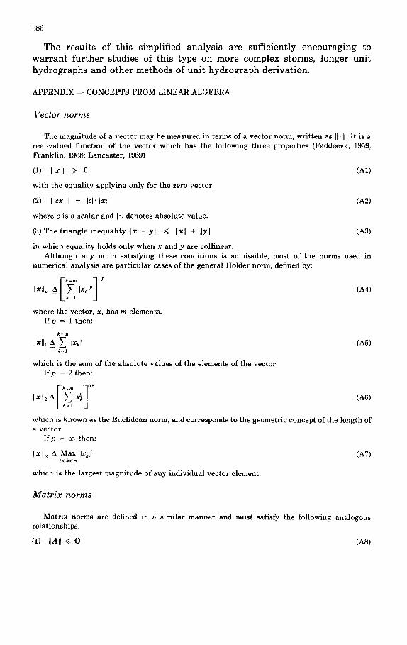
V e c t o r n o r m s

The magni tude of a vec tor may be measured in te rms of a vec tor norm, wr i t t en as ]1" H. It is a real-valued func t ion of the vec tor which has the following th ree proper t ies (Faddeeva, 1959; Frankl in , 1968; Lancas te r , 1969)

(1) [I xl l ~> 0 (A1)

wi th the equal i ty apply ing only for the zero vector .

(2) II cx II = Icl" Ilxtl (A2)

where c is a sca lar and I'l denotes absolute value.

(3) The t r iangle inequal i ty IIx + Yll ~< Ilxll + IfYll (A3)

in which equal i ty holds only when x and y are coll inear. A l though any norm sat isfying these condi t ions is admissible, most of the norms used in

numer ica l analys is are pa r t i cu la r cases of the genera l Holder norm, defined by:

rk=m 71/P Ilxlt, a__ L ~1 tx.l'J (A4)

where the vector , x, has m elements . I f p = 1 then:

k m

][Xlll A ~ Ixkl (A5) k - 1

which is the sum of the absolute values of the e lements of the vector . I f p = 2 then:

Ilxrl2 _ k k=~ ~ (A6)

which is known as the Euclidean norm, and corresponds to the geometric concept of the length of a vector.

I fp = oo then:

Hx][~ A Max [xk]' (A7) l~k<~m

which is the largest magn i tude of any individual vec tor element .

M a t r i x n o r m s

Matr ix norms are defined in a s imilar manne r and must sat isfy the fol lowing analogous re la t ionships .

(1) IIAII < 0 (AS)

387

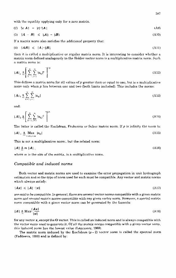
wi th the equa l i ty app ly ing only for a zero ma t r ix .

(2) Iic All = Icl"qlAhl (A9)

(3) IIA + B]I ~< IhAll + IIBIb (AI0)

If a m a t r i x n o r m also sa t is f ies t he add i t iona l p roper ty tha t :

(4) IIABII ~ I]A[['IIBI[ (Al l )

t h e n it is ca l led a mu l t ip l i ca t ive or r egu l a r m a t r i x norm. It is i n t e r e s t i ng to cons ider w h e t h e r a ma t r i x n o r m defined a n a l o g o u s l y to t he Holder vec to r n o r m is a mul t ip l i ca t ive ma t r i x norm. Such a ma t r i x n o r m is:

IIA]lp A lakj I" (A12)

Th i s def ines a m a t r i x n o r m for all v a l ue s o f p g r ea t e r t h a n or equal to one, bu t is a mul t ip l i ca t ive no rm only w h e n p lies be tween one and two (both l imi ts included) . Th i s inc ludes the norms:

I,A[I, A ~ ~ la~jl (113) k 1 J ~ l

and:

10- blA]l~ A lake[ ~ (A14) I_k:l j : l

The l a t t e r is ca l led t he Euc l idean , F roben i u s or S c h u r m a t r i x norm. I f p is inf in i ty t he n o r m is:

liAIl~_ A M a x lakj I (A15) l<~k,j<~m

This is no t a mul t ip l i ca t ive norm:, bu t the r e l a t ed norm:

I[AI] A m IIAII ~ (A16)

where m is t he size of t he ma t r ix , is a mul t ip l i ca t ive norm.

Compat ib le a n d i nduc e d norms

Both vec to r and ma t r i x n o r m s are used to e x a m i n e t he e r ro r p r o p a g a t i o n in un i t h y d r o g r a p h e s t i m a t i o n and so the type of n o r m used for each m u s t be compat ible . A n y vec to r and ma t r i x n o r m s wh ich a lways sat isfy:

]lAxll <~ ][AIl.llxll (A17)

a re said to be compat ible . In genera l , t h e r e a re seve ra l vec to r n o r m s compat ib le wi th a g iven ma t r i x n o r m and severa l m a t r i x n o r m s compat ib le wi th any g iven vec tor norm. However , a special ma t r i x no rm compat ib le wi th a g iven vec to r n o r m can be gene ra t ed by the formula:

IIAII A Max I[Ax[I (A18) - ]lxll

for any vec to r x, except t he O vector . Th i s is ca l led an induced n o r m and is a lways compat ib le wi th the vec to r n o r m used to g e n e r a t e it. Of all t he m a t r i x n o r m s compat ib le wi th a g iven vec to r norm, th i s induced n o r m h a s t he lowest va l ue (Lancas te r , 1969).

The m a t r i x n o r m induced by t he E u c l i d e a n (p= 2) vec to r n o r m is cal led the spec t ra l no rm (Faddeeva , 1959) and is defined by:

388

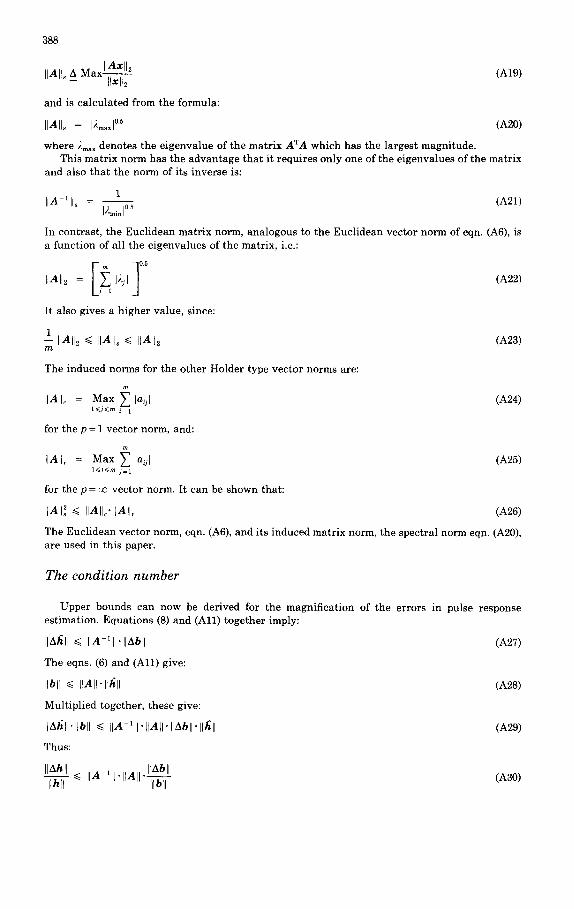
[IAII~ A Max IlAxl[2 - I t x l t ~

and is ca lcu la ted from the formula:

Ilall~ = 12m~l °-5

(A19)

(A20)

IBA~H ~< ]]A ~l[.[[Ab[[ (A27)

The eqns. (6) and ( A l l ) give:

I[bdl ~< IPA]P-]Ih[[ (A28)

Mul t ip l i ed toge ther , these give:

llahll • Ilblj ~< IIA -~ II'ldAtl" II~bl[" IIhll (A29)

Thus:

[[Ah![ IJAb[[ I]h]-~- ~< IIA ~ll'l[All ° ]lb]] (A30)

where 2max deno tes the e igenva lue of the ma t r ix A~rA which has the la rges t magni tude . This m a t r i x no rm h as the a d v a n t a g e t h a t i t r equ i res only one of the e igenva lues of the ma t r ix

and also t h a t the norm of i ts inverse is:

1 ]JA l Jd~ (A21)

I ) . ~ in l °.5

In cont ras t , t he Euc l idean ma t r ix norm, ana logous to the Euc l idean vec tor norm of eqn. (A6), is a func t ion of all the e igenva lues of the matr ix , i.e.:

0.5

HAl,2 = [_i %'~ [~j, (A22)

It also gives a h ighe r value, since:

1 - - [JAi l 2 ~< []A[] s ~< []All 2 (A23) m

The induced norms for the o the r Holder type vec tor norms are:

d[A[[c = Max ~ [alj [ (A24) l<~j<<.m z~= 1

for the p = 1 vec to r norm, and:

I[AlJr = Max ~ lai1 [ (A25) l < ' i ~ m j ~ l

for the p = ~ vec to r norm. It can be shown tha t :

HAI[~ ~< []Al[c.l]APlr (A26)

The Euc l idean vec tor norm, eqn. (A6), and its induced mat r ix norm, the spec t ra l no rm eqn. (A20), are used in th i s paper.

The condition number

Upper bounds can now be der ived for the magni f i ca t ion of the e r rors in pulse response es t imat ion . Equa t i ons (8) and ( A l l ) t oge the r imply:

389

which relates the relative error in the estimated uni t hydrograph to the relative error in the output vector. The quantity:

K(A) A I]A-'ll" IIAIq (A31)

is an upper bound for the amplification and is called the condition number of the matrix A. For the spectral norm, this is given by:

"~rnax 0.5 K(A) = ~ (A32)

An error m the input time-series, hence in the matr ix A, causes an estimation error of:

Ah = [(A + AA)- ' - A-1lb (A33)

The identity:

C 1 _ D 1 =_ D -~(D - C)C -1 (A34)

can be used to write eqn. (A33) as:

Ah A ~( AA)(A + AA) l b A ~(A - AA) (h + Ah) (A35)

It follows that:

IIAhll IIAAll IIAall ~< IIA 'll'llAII llAI---~ = K(A) IIAI--~- (A36)

so tha t the amplification of this type of error is controlled by the same condition number as in case of error in the output vector. The corresponding formula for the case of errors in both the input and output vectors is:

]IAhII<<.K(A)I(~ 1 t IIAAII [[Abll 1 [IAAli] IIAI[ + ~ (A37) IIhll - K(A) ~ - ~ /

Note tha t each choice of matrix and vector norm may give a different value for the condition number, but if the same norms are used consistently to examine different estimation methods, or input vectors, the ranking remains the same for any choice of norms.

REFERENCES

Barnes, B.S., 1959. Consistency in uni t hydrographs. Proc. ASCE, (HY8): 39-63. Box, G.E.P. and Jenkins, G.M., 1970. Time-series analysis: forecasting and control. Holden Day,

San Francisco, Calif. Bruen, M., 1977. A comparison of some methods of l inear system identification. Intern. Rep., Civ.

Eng. Dep., Universi ty College, Dublin. Bruen, M., 1985. Black-box methods of systems analysis applied to modelling of ca tchment

behaviour. Ph .D. Thesis, National Universi ty of Ireland. Bruen, M. and Dooge, J.C.I. 1984. An efficient and robust method for est imating unit hydrograph

ordinates. J. Hydrol., 70: 1-24. Collins, W.T., 1939. Runoff distr ibution graphs from precipitat ion occurring in more than one time

unit. Civ. Eng., 9(9): 559-561. Dooge, J.C.I., 1965. Analysis of l inear systems by means of Laguerre functions. J. SIAM Control,

Ser. A., 2(3): 39~408.

390

Dooge, J.C.I., 1973. Linear theory of hydrological systems. Tech. Bull. No. 1468, U.S. Dep. Agric. Dooge, J.C.I., 1979. Deterministic input-output models. In: E.H. Lloyd, T. O'Donnell and J.C.

Wilkinson (Editors), Mathematics of Hydrology and Water Resources, Academic Press, London.

Dooge, J.C.I. and Bruen, M., 1978. Linear algebra and unit hydrograph stability. Int. Symp. Hydrol. Water Resour., Simon Bolivar University, Caracas.

Dooge, J.C.I. and Garvey, B.J., 1978. The use of Meixner functions in the identification of heavily- damped systems. Proc. R. Irish Acad., A78(18): 157-179.

Eagleson, P.S., Mejia, R. and March, F., 1966. Computation of optimum realizable unit hydrographs. Water Resour. Res., 2(4): 755~764.

Faddeeva, V.N., 1959. Computational methods of linear algebra. Dover Publ. New York, N.Y. Franklin, J.N., 1968. Matrix Theory. Prentice Hall, Englewood Cliffs, N.J. Garvey, B.3., 1972. An analysis of linear systems by means of Laguerre and Meixner functions. M.

Eng. Sci., Thesis, University College, Dublin. Kuchment, L.S., 1967. Solution of inverse flow problems for linear flow models. Sov. Hydrol., Sel.

Pap., 2: 194-199. Lancaster, P., 1969. Theory of Matrices. Academic Press, New York, N.Y. Laurenson, E.M. and O'Donnell, T., 1969. Data error effects on unit hydrograph derivation. Proc.

ASCE, HY6: 189~1917. Linsley, R.K., Kohler, M.A. and Paulhus, J.L.H., 1949. Applied Hydrology. McGraw-Hill, New

York, N.Y. O'Donnell, T., 1960. Unit hydrograph derivation by harmonic analysis. IAHS Publ. 51: 546-557. Tikhonov, A.N., 1965. Improperly posed problems of linear algebra and a stable method for their

solution. English transl, in Sov. Math., 6: 988-991.