journal 25 200903
DESCRIPTION
The Journal on financial transformation, edited by The Capital Markets Company (Capco), produced by Cypres. Capco is a leading global provider of integrated consulting, technology, and transformation services dedicated solely to the financial services industry. Recipient of the APEX Awards for Publication Excellence 2002 & 2008TRANSCRIPT

journal 03
/20
09
/#2
5
the journal of financial transformation
www.capco.com
Amsterdam T +31 20 561 6260
Antwerp T +32 3 740 10 00
Bangalore T +91 80 4199 7200
Frankfurt T +49 69 9760 9000
Geneva T +41 22 819 1774
London T +44 20 7426 1500
New York T +1 212 284 8600
Paris T +33 1 77 72 64 40
San Francisco T +1 415 445 0968
Toronto T +1 416 923 4570
the journal of fi
nancial transformation
03/20
09/#
25
Recipient of the APEX Awards for Publication Excellence 2002-2008
Cass-Capco Institute Paper Series on Risk

www.capco.com
Amsterdam T +31 20 561 6260
Antwerp T +32 3 740 10 00
Bangalore T +91 80 4199 7200
Frankfurt T +49 69 9760 9000
Geneva T +41 22 819 1774
London T +44 20 7426 1500
New York T +1 212 284 8600
Paris T +33 1 77 72 64 40
San Francisco T +1 415 445 0968
Toronto T +1 416 923 4570
the journal of fi
nancial transformation
03/20
09/#
25

Editor
Shahin Shojai, Global Head of Strategic Research, Capco
Advisory Editors
Dai Bedford, Partner, Capco
Nick Jackson, Partner, Capco
Keith MacDonald, Partner, Capco
Editorial Board
Franklin Allen, Nippon Life Professor of Finance, The Wharton School,
University of PennsylvaniaJoe Anastasio, Partner, Capco
Philippe d’Arvisenet, Group Chief Economist, BNP Paribas
Rudi Bogni, former Chief Executive Officer, UBS Private Banking
Bruno Bonati, Strategic Consultant, Bruno Bonati Consulting
David Clark, NED on the board of financial institutions and a former senior
advisor to the FSA
Géry Daeninck, former CEO, Robeco
Stephen C. Daffron, Global Head, Operations, Institutional Trading & Investment
Banking, Morgan Stanley
Douglas W. Diamond, Merton H. Miller Distinguished Service Professor of Finance,
Graduate School of Business, University of Chicago
Elroy Dimson, BGI Professor of Investment Management, London Business School
Nicholas Economides, Professor of Economics, Leonard N. Stern School of
Business, New York University
José Luis Escrivá, Group Chief Economist, Grupo BBVA
George Feiger, Executive Vice President and Head of Wealth Management,
Zions Bancorporation
Gregorio de Felice, Group Chief Economist, Banca Intesa
Hans Geiger, Professor of Banking, Swiss Banking Institute, University of Zurich
Wilfried Hauck, Chief Executive Officer, Allianz Dresdner Asset Management
International GmbH
Pierre Hillion, de Picciotto Chaired Professor of Alternative Investments and
Shell Professor of Finance, INSEAD
Thomas Kloet, Senior Executive Vice-President & Chief Operating Officer,
Fimat USA, Inc.
Mitchel Lenson, former Group Head of IT and Operations, Deutsche Bank Group
David Lester, Chief Information Officer, The London Stock Exchange
Donald A. Marchand, Professor of Strategy and Information Management,
IMD and Chairman and President of enterpriseIQ®
Colin Mayer, Peter Moores Dean, Saïd Business School, Oxford University
Robert J. McGrail, Executive Managing Director, Domestic and International Core
Services, and CEO & President, Fixed Income Clearing Corporation
John Owen, CEO, Library House
Steve Perry, Executive Vice President, Visa Europe
Derek Sach, Managing Director, Specialized Lending Services, The Royal Bank
of Scotland
John Taysom, Founder & Joint CEO, The Reuters Greenhouse Fund
Graham Vickery, Head of Information Economy Unit, OECD
Norbert Walter, Group Chief Economist, Deutsche Bank Group


TABlE of conTEnTs
PArT 1
8 opinion — Delta hedging a two-fixed-income-securities portfolio under gamma and vega constraints: the example of mortgage servicing rightsCarlos E. Ortiz, Charles A. Stone, Anne Zissu
12 opinion — reducing the poor’s investment risk: introducing bearer money market mutual sharesRobert E. Wright
15 opinion — financial risk and political risk in mature and emerging financial marketsWenjiang Jiang, Zhenyu Wu
19 Estimating the iceberg: how much fraud is there in the U.K.?David J. Hand, Gordon Blunt
31 Enhanced credit default models for heterogeneous sME segmentsMaria Elena DeGiuli, Dean Fantazzini, Silvia Figini, Paolo Giudici
41 The impact of demographics on economic policy: a huge risk often ignoredTimothy J. Keogh, Stephen Jay Silver, D. Sykes Wilford
51 risk and return measures for a non-Gaussian worldMichael R. Powers, Thomas Y. Powers
55 Medium-term macroeconomic determinants of exchange rate volatilityClaudio Morana
65 risk adjustment of bank stocks in the face of terrorDirk Schiereck, Felix Zeidler
75 Macroeconomic risk — sources and distributions according to a DsGE model of the E.U.David Meenagh, Patrick Minford, Michael Wickens
PArT 2
88 opinion — risk management in the evolving investment management industryPhilip Best, Mark Reeves
91 opinion — Bridging the gap — arbitrage free valuation of derivatives in AlMPeter den Iseger, Joeri Potters
95 Does individual performance affect entrepreneurial mobility? Empirical evidence from the financial analysis marketBoris Groysberg, Ashish Nanda, M Julia Prats
107 A new approach for an integrated credit and market risk measurement of interest rate swap portfoliosJohn Hatgioannides, George Petropoulos
113 risk drivers in historical simulation: scaled percentage changes versus first differencesSu Xu, Stephen D. Young
123 The impact of hedge fund family membership on performance and market shareNicole M. Boyson
131 Public sector support of the banking industryAlistair Milne
145 Evaluating the integrity of consumer payment systemsValerie Dias
155 A loss distribution for operational risk derived from pooled bank lossesManMohan S. Sodhi, Wayne Holland

No one can deny that the extent and ferocity of the events of the past year or so have been unexpected. We all
went from having minor fears about an economic slowdown in Western economies, with the East somewhat shielded
and a manageable crisis within the financial sector, to a situation where many are talking about a potential global
depression and nationalization of most of the world’s major financial institutions. Everyday we are faced with even
more worrying news. Yet despite the uncertainty, now is when we need a clear head and ideas about what must be
done to survive, and possibly even prosper.
When this paper series with Cass Business School was established in early 2007, we were convinced that many in
the financial services sector underestimated the risks inherent in many of the instruments and transactions they
were counterparty to, and that more financial discipline was needed to benefit from the array of innovations taking
place. We highlighted a number of these concerns in the inaugural issue of the paper series and feel vindicated by
the events that have transpired since.
The establishment of this paper series exemplifies the reason we founded Capco in the first place, namely to help the
industry in ways that were not previously possible. To help the industry recognize that fascinating formulas don’t
necessarily represent accuracy, that operational risk is endemic, and that we have all got a long way to go before
we come to grips with the risks each institution faces and the most effective ways of managing them.
This second edition of the Cass-Capco Institute Paper Series on Risk covers the whole spectrum of financial sector
risks. A number of papers focus on how risk could be better understood, measured, and managed. The paper series
comes to life during our annual conference on April 6th at the Cass Business School, where we hope to see many
of you.
The challenges facing our industry have never been greater. That is why publications such as this are essential. We
need to take a critical view of what went wrong, objectively identify where the shortfalls are, and ensure that we
correct them for the future. These are the objectives of this issue, and have always been the ambitions of Capco
and its partners.
It is only through a better understanding of the past that we can make a brighter future. We hope that we have also
been able to contribute in our own way to that journey. Obviously, we still have a long way to go before we achieve
what we set out to do when we established Capco. But we shall stand shoulder to shoulder with our clients in ensur-
ing that our industry achieves the levels of efficiency that we are certain it deserves. Our hope is that you will also
join us in helping shape the future of our industry.
Good reading and good luck.
Yours,
Rob Heyvaert,
Founder and CEO, Capco
Dear reader,

After 40 years of growing confidence about our understanding of risk, many are now questioning the basic
fundamentals of how it should be measured, let alone managed. Ever since the options pricing model was
developed, so-called financial experts have been engineering exciting new instruments for the financial markets.
As the complexity and variety of these instruments grew so did the thirst of the investment community for them.
This helped create a vicious circle of demand and hubris. The last 40 years were the hubris years.
It was not only in the financial markets that hubris over our understanding of the functioning of the models
prevailed. Economists genuinely believed that they understood how economies operate and had developed models
that could influence them. Economists at the IMF sincerely thought that they understood how economic tools could
be applied and were certain of their implications.
The events of the past two years have forced everyone to take a step back and reassess their models. Everyone
has now realized that the world of economics is far too complex for anyone to be able to influence; that financial
risk is dependent on far too many variables to be correctly measured; and that the certainty with which financial
and economic experts spoke had no relationship to reality.
We were aware of the risks that were inherent within the global financial system when we first established the
Cass-Capco Institute Paper Series on Risk, and hoped that better dialogue between the world of finance and
academia would help mitigate them. However, we had no idea that our timing was so perfect, that we were fast
approaching the end of the hubris era.
We were not alone in getting caught out by the speed with which many of the stars of the world of economics and
finance lost their reputations. Many authors in this issue had no idea when thinking about their articles that they
would be so pertinent at the time of publication.
The papers in this edition highlight many of the problems that exist within the models used and provide insights
into how they can be mitigated in the future. The topics covered are broad, ensuring that we discuss as many
economic areas as possible.
We hope you enjoy reading these articles and that you also make your own contribution by submitting articles to
future issues of the Journal.
On behalf of the board of editors
The end of hubris


Part 1
Delta hedging a two-fixed-income-securities portfolio under gamma and vega constraints: the example of mortgage servicing rights
Reducing the poor’s investment risk: introducing bearer money market mutual shares
Financial risk and political risk in mature and emerging financial markets
Estimating the iceberg: how much fraud is there in the U.K.?
Enhanced credit default models for heterogeneous SME segments
The impact of demographics on economic policy: a huge risk often ignored
Risk and return measures for a non-Gaussian world
Medium-term macroeconomic determinants of exchange rate volatility
Risk adjustment of bank stocks in the face of terror
Macroeconomic risk — sources and distributions according to a DSGE model of the E.U.

Since July 2007, we have witnessed a growing number of mortgages
going into default and eventually being foreclosed. Mortgage servic-
ing rights are fees collected by institutions managing mortgages. The
yearly fees correspond to a percentage of the outstanding balance
of individual mortgages. Typically, an institution collects between 25
and 50 basis points per year (.25%-.5% of the outstanding balance
each year). The servicing is a compensation that institutions receive
for services that include the collection of the monthly payments, for
making sure that the monthly payments are paid on time, and, when
necessary, for foreclosing the property when a mortgagor defaults
on the property. Banks have been confronted with major losses
related to mortgage-backed securities and to the heavy reduction in
the volume of mortgage servicing rights.
Ortiz et al. (2008) develop a dynamical hedge ratio for portfolios of
mortgage servicing rights (MSR) and U.S. Treasury securities, such
that it is readjusted for changes in market rates and prepayment
rates. They develop a delta-hedge ratio rebalancing function for
three different portfolios, compare the three dynamic hedge ratios,
and rank them with respect to the gamma hedge ratio.
In this paper we develop a general model to obtain the optimal delta
hedge for a portfolio of two-fixed-income-securities (a1, a2), each
a function of the market interest rate y, such that when the value
of each of the individual securities changes up or down, because
of changes in market rates y, the total value of the portfolio is
unchanged. We develop the delta hedge under the constraint of a
zero-gamma in order to avoid costs related to the rebalancing of
such portfolio.
We first describe in details mortgage servicing rights (MSR), then
we develop the model, and finally discuss how our model can be
applied to MSR.
Mortgage servicing rightsBecause MSRs correspond to a percentage of the mortgages’
outstanding balance their characteristics are the same as those of
interest only (IOs). IO securities have values that are both affected
by interest rates and prepayment rates. It is interesting to analyze
the price/yield relationship of an IO security in order to understand
MSRs.
Figure 1 shows the projected scheduled principal (at the very bot-
tom), the unscheduled principal, the interest, and servicing (top)
to be paid over time for a 5.5%-FNMA pass-through security. The
pass-through security is backed by a pool of mortgages with a cur-
rent balance of U.S.$52 million, a weighted average maturity of
28.8 years, and a weighted average coupon rate of 6.243%. The
cash flows are based on a projected PSA of 50, which corresponds
to an annual prepayment rate of 3% (cpr = 3%).
Because the graph in Figure 2 is compressed, it is important, when
comparing it to Figure 1, to read the numbers on the vertical axis.
Figure 2 shows what happens to the different projected cash flows
for a projected 1000 PSA (60% annual prepayment rate). Clearly,
the total principal being repaid overtime remains the same (same
area under the curve) under the two different prepayment scenari-
os, however, both the interest and servicing are being significantly
reduced for faster prepayment rate. When principal is refinanced,
no more interest is paid by mortgagors and banks cannot collect
servicing fees for mortgages that do not exist anymore.
Prepayment rates are a function of interest rates. When interest
rates decrease, prepayment rate increases and vice versa. Figure
3 graphs the projected cash flows of an IO security over time, for
different prepayment scenarios.
Figure 3 is taken from Bloomberg and shows the cash flows of a 9%
FHS IO under four different PSA scenarios. CPR stands for constant
prepayment rate. A CPR of 5% indicates that mortgage principal
is being prepaid at an annual rate of 5%. The prepayment model
developed by the Public Securities Association (PSA) is also widely
used for a basis of quoting prices on mortgage-backed securities.
A 100 PSA corresponds to a 6% cpr, a 200 PSA corresponds to a
12% cpr, and a 500 PSA corresponds to a 30% cpr. In the Figure,
PSA ranges from 0% to 395%. When PSA rate is high, more of the
outstanding balance is being prepaid, so less IO or MSR is available
as a percentage of outstanding remaining balance. This can be
Delta hedging a two-fixed-income-securities portfolio under gamma and vega constraints: the example of mortgage servicing rights Carlos E. Ortiz, Chairman, Department of Computer Science and Mathematics, Arcadia University
Charles A. Stone, Associate Professor, Department of Economics, Brooklyn College, City
University of New York
Anne Zissu, Chair of Department of Business, CityTech, City University of New York, and Research
Fellow, Department of Financial Engineering, The Polytechnic Institute of New York University
8 – The journal of financial transformation

observed for example under PSA 395, the lowest curve in Figure 3.
On the other hand, for low PSA, the outstanding balance remains
at a greater level, and the derived cash flows stay higher (see top
curve for extreme scenario of 0 PSA).
It is important that the reader understands that the value of an IO,
or of a MSR, is the present value of the cash flows received over
time. Clearly, the lower the cash flows are (due to high prepayment
rates), the lower the value is. On the other hand, the higher the cash
flows are, due to high market interest rates and therefore low pre-
payment rates, the higher the value is. This is true only over a range
of interest rates (prepayment effect). At some point, however, the
discount effect takes over the prepayment effect, and the value of
IOs or MSRs will start to decrease. We show the typical value of an
IO or MSR as a function of interest rates in Figure 4.
The value of an IO security or a MSR increases when interest rates
(y) increase as long as the prepayment effect is greater than the
discount effect. When the discount effect takes over, we observe
the value decreasing for increases in interest rates. Both IOs and
MSRs are very interesting types of securities. Most fixed income
securities decrease in value when yields increase. IOs and MSRs do
the opposite for a wide range of yields.
s-curve prepayment functionIt is important to understand the prepayment behavior in order to
value MSR. Periodically, investment banks submit to Bloomberg
their expected PSA level for corresponding changes in yield.
Figure 5 shows the data submitted by twelve investment banks
on their expected PSA levels for corresponding changes in yields
ranging from -300 bps to +300 bps, for the same 5.5% FNMA
pass-through security we described in the beginning of the paper
with Figures 1 and 2. It is interesting to observe how different
these projections can be. For a decrease of 300 bps, the projected
PSA ranges from 884 to 3125 (a corresponding cpr ranging from
53% to 187.6%).
9
Figure 1 Figure 3
Figure 2 Figure 4

10 – The journal of financial transformation
Figure 6 plots for different changes in yield, the corresponding
expected PSA level for each investment bank that submitted
information to Bloomberg on October 2008 for a specific pool of
securitized mortgages. The changes in yield are represented on the
horizontal axis, with expected PSA levels on the vertical axis. The
curve represents the median for the twelve banks that submitted
the data. One can see that the prepayment curve, as a function of
changes in yield, has an S-shape. The S-shape prepayment function
is common to all banks, but each differs in projecting its magnitude/
steepness.
The S-curve shows a steeper slope around the initial market rate
(at 0% change in yield), with prepayment rate increasing as mar-
ket rates continue to drop, until a burnout effect is reached, and
the curve flattens, meaning that prepayment rate is no longer
increasing as it did in the middle range of market rates decrease.
The S-curve also flattens in the high range of market rates. What
happens is that prepayment rate decreases with increase in market
rates until it reaches a minimum beyond which no further decrease
in prepayment rates is observed. The natural level of prepayment
rate is reached, that is, the prepayment rate that is independent of
market rates, but is a function of mortgagers’ personal events.
We next, express the relationship between prepayment rate (we
use cpr for prepayment rate instead of PSA) and the change in
basis points. The prepayment rate, cpr, is mainly a function of the
difference between the new mortgage rate y in the market and the
contracted mortgage rate r. cpr = a ÷ [1 + eb(y-r)].
We now develop a general model for a two-fixed-income-security
portfolio that is delta and gamma hedged against interest rate
changes.
Model for portfolio optimizationWe have a portfolio of two securities (a1, a2). Each security's value
is a function of the market interest rate y. We want to find the opti-
mal share of each security in the portfolio such that: Σi=k→2 αiai = K
(1), where αi is the weight of security ai. In order for the value K of
the portfolio, at a specific yield y, to be hedged against any move-
ments in interest rate we need to find the optimal weights for each
security in the portfolio, such that when there is a change in market
rates the sum of the change in value of each security times its cor-
responding weight in the portfolio is equal to zero.
We next, develop a general model and apply it to the particular case
of portfolios of mortgage servicing rights (MSRs). Consider two
functions ai(y), i = 1,2 and two coefficients αi, i = 1,2. We want the
following to hold: Σi=1→2 αiai(y) = K (2).
The values of the functions ai(y) are given for every value of y and
we want to find the values of αi that will satisfy equation (2), and
other conditions of ‘stability’ that we will describe later.
notation: For any ƒ(y) let us denote by ƒ(n)(y) the n-th derivative
of ƒ.
When the αi’s are assumed to be constant, the objective is to find
for a fixed y0, hence for any given value of the ai(y0), values of the
constants αi, such that: Σi=1→2 αiai(y0) = K (3).
[Σi=1→2 αiai(y0)]1 = [Σi=1→2 αiai(1)(y0)] = 0 (4), where the second con-
dition represents the constraint that the total sum of the αiai(y0)
will not change for small changes in y from the initial value y0.
More generally, to obtain an optimal portfolio we need to find the
values of the αi for i = 1,2 such that for small changes in y from
the original y0, the value of Σi=1→2 αiai(y) will not change from the
original value of Σi=1→2 αiai(y0) = K.
Figure 5
Figure 6

11
For a fixed y0 there exists a unique solution that optimizes the port-
folio of two fixed income securities if: a1(y0)a2(1)(y0) – a1
(1)(y0)a2(y0)
≠ 0. As expected, this condition depends only on the values of the
functions a1, a2 and their derivatives at point y0. The values for α1
and α2, the optimal weights for the two securities that constitute a
delta-gamma hedged portfolio, are:
α1 = [Ka2(1)(y0)] ÷ [a1(y0)a2
(1)(y0) – a1(1)(y0)a2(y0)]
α2 = [-Ka1(1)(y0)] ÷ [a1(y0)a2
(1)(y0) – a1(1)(y0)a2(y0)]
If: a1(y0)a2(1)(y0) – a1
(1)(y0)a2(y0)] = 0
Then we have no solutions or there exist infinitely many solutions.
Examples of no solutionsIt is not unusual to have a portfolio of fixed-income securities that
increases in value when market rates decline and decreases in
value when market rates rise. We could have, for example, a portfo-
lio composed of a 30-year 8% coupon bond with a 10-year Treasury
note. This is a case when it is impossible to delta hedge the portfolio
under gamma and vega constraints.
The case of mortgage servicing rightsA delta-hedged portfolio could have a combination of bonds and MSR.
We next present the valuation approach developed by Stone and
Zissu (2005) that incorporates the prepayment function (S-curve).
Valuation of Msr
The cash flow of a MSR portfolio at time t is equal to the servicing
rate s times the outstanding pool in the previous period: MSRt =
(s)m0(1 – cpr)t-1Bt-1 (5), where m0 is the number of mortgages in
the initial pool at time zero, B0 is the original balance of individual
mortgage at time zero, r is the mortgage coupon rate, cpr is the
prepayment rate, m0(1-cpr)t is the number of mortgages left in pool
at time (t), Bt is the outstanding balance of individual mortgage at
time (t), and s is the servicing rate.
V(MSR) = (s)m0 [Σ(1 – cpr)t-1Bt-1] ÷ [(1+y)t] (6), with t = 1,…..n (through
the entire paper)
Equation (6) values a MSR portfolio by adding each discounted cash
flow generated by the portfolio to the present, where n is the time
at which the mortgages mature, and y is the yield to maturity.
After replacing the prepayment function in equation (6) we obtain
the MSR function as:
V(MSR) = (s)m0 [Σ(1 – (a/(1+expb(y-r)))t-1Bt-1] ÷ [(1+y)t] (6a)
Valuation of a bond
The valuation of a bond with yearly coupon and face value received
at maturity is represented in equation (4): V(B) = c Σ1/(1+y)t + Face/
(1+y)t (7), where V(B) is the value of a bond, c is the coupon, Face
is the face value, n is the time at which the bond matures, and y is
the yield to maturity.
If we now relabel equation (6a) and equation (7) as a1 and a2 respec-
tively, and replace them in the equations we derived previously for
the optimal α1 and α2 respectively, we obtain a portfolio of bonds
and of MSR that is delta- and gamma-hedged against small changes
in interest rates and corresponding changes in prepayment rates.
conclusionWith an estimated $10 trillion in outstanding mortgages, MSR gen-
erate a significant source of income for banks. This is a significant
market with risks that need to be addressed. If not managed prop-
erly, banks will have important losses to report. Prepayment risk
and interest rate risks need to be carefully evaluated when creating
a portfolio of fixed income securities. We have developed a gen-
eral portfolio of two-fixed-income securities, each with the optimal
weight, in order for the portfolio to be delta- and gamma-hedged
against small changes in interest rates. We have shown how this
model can be applied to portfolios’ MSR.
references• Bierwag, G. O., 1987, “Duration analysis: managing interest rate risk,” Ballinger
Publishing Company, Cambridge, MA
• Boudoukh, J., M. Richardson, R. Stanton, and R. F. Whitelaw, 1995, “A new strategy for
dynamically hedging mortgage-backed securities,” Journal of Derivatives, 2, 60-77
• Ederington, L. H., and W. Guan, 2007, “Higher order Greeks,” Journal of Derivatives,
14:3, 7-34
• Eisenbeis, R. A., S. W. Frame, and L. D. Wall, 2006 “An analysis of the systemic risks
posed by Fannie Mae and Freddie Mac and an evaluation of the policy options for
reducing those risks,” Federal Reserve Bank of Atlanta, Working Paper Series, Working
Paper 2006-2
• Goodman, L. S., and J. Ho Jeffrey, 1997, “Mortgage hedge ratios: which one works
best?” Journal of Fixed Income, 7:3, pp 23-34
• Mato, M. A. M., 2005, “Classic and modern measures of risk in fixed-income portfolio
optimization,” Journal of Risk Finance, 6:5, 416-423
• Office of Thrift Supervision, 2007, “Hedging mortgage servicing rights,” Examination
Book, 750.46-750.52, July
• Posner K., and D. Brown, 2005, “Fannie Mae, Freddie Mac, and the road to redemp-
tion,” Morgan Stanley, Mortgage Finance, July 6
• Ortiz, C. E., C. A. Stone, and A. Zissu, 2008, “Delta hedging of mortgage servicing port-
folios under gamma constraints,” Journal of Risk Finance, 9:4
• Ortiz, C. E., C. A. Stone, and A. Zissu, 2008, “Delta hedging a multi-fixed-income-securi-
ties portfolio under gamma and vega constraints,” Journal of Risk Finance, forthcoming
• Stone, C. A. and A. Zissu, 2005, The securitization markets handbook: structure and
dynamics of mortgage- and asset-backed securities, Bloomberg Press
• Yu. S. K., and A. N. Krasnopolskaya, 2006, “Selection of a fixed-income portfolio,”
Automation And Remote Control, 67:4, 598 – 605

12 – The journal of financial transformation
reducing the poor’s investment risk: introducing bearer money market mutual sharesRobert E. Wright, Clinical Associate Professor of Economics, Department of Economics, Stern School of Business, New York University
Now that micro-credit in general and the Grameen Bank in particular
have finally received their due recognition [Yunus and Jolis (1998)],
policymakers and international financiers can begin to focus on the
other side of the poor’s balance sheet, their assets or savings. As de
Soto (2000) and others have pointed out, property rights in many
countries remain precarious and formal protection of physical and
intellectual property costly. In many places, not even the local curren-
cy can be trusted to hold its value for any significant length of time.
Billions of people therefore have little ability or incentive to save.
Outsiders cannot impose democracy or property rights protections
[Baumol et al. (2007)] and, as Stiglitz (2002), Easterly (2006), and
others have argued, the IMF and World Bank can do precious little
to thwart bouts of inflation, exchange crises, and financial panics in
developing countries. Outsiders can, however, provide the world’s
poor with a safe, low transaction cost, and remunerative savings out-
let. For several generations, poor people in many places throughout
the globe have saved by buying U.S. Federal Reserve notes and the
fiat currencies of other major economic powers. Although subject to
physical risk (theft, burning, and so forth) and exchange rate fluctua-
tions, such notes typically held their purchasing power much better
than local notes or bank deposits denominated in local currencies. As
the dollar weakens over the next few decades, as most expect it to
do as the U.S. economy loses ground relative to Europe, a revitalized
Japan, and the BRIC nations, its allure as a savings vehicle will fade.
International financiers can fill the vacuum with a simple product,
bearer money market mutual shares (B3MS), almost guaranteed to
appreciate against all the world’s fiat monies.
reducing the poor’s investment risk: introducing bearer money market mutual sharesHelping budding entrepreneurs to obtain loans, even for just a
few dollars, is beyond noble. It is growth-inducing. Where oligarchs
or the grabbing hand of government [Shleifer and Vishny (1998)]
are not overpowering, micro-credit can summon forth productive
work where before was only despair [Aghion and Morduch (2005),
Khandker (1998), Yunnis and Jolis (1998)]. Micro-insurance is also
gaining traction [Mijuk (2007)]. But what becomes of the entre-
preneur who thrives and begins to accumulate assets? The small
businessperson who, for any number of valid reasons, may not want
to continue plowing profits back into her business? Who fears pur-
chasing conspicuous physical assets lest they be seized by the state
or brigands? Who wishes to avoid investing in financial assets issued
by shaky, inept, or corrupt local intermediaries or denominated in a
local currency of dubious value over the desired holding period, be it
a week, month, year, or decade?
For the past several generations and up to the present, millions of
such people worldwide have invested in U.S. Federal Reserve notes
or the physical media of exchange of other major nations. Although
subject to some physical risk of theft, loss, burning, and the like, the
high value to bulk of such notes renders them ideal for saving for a
personal rainy day or hedging against a local economic meltdown.
Returns in terms of local purchasing power are not guaranteed, but
Federal Reserve notes are perfectly safe from default risk and highly
liquid, sometimes even more liquid than local notes or deposits. Their
widespread use as personal savings and business working capital
attests to the financial savvy of people worldwide [Allison (1998)].
The U.S. dollar has often been the best available savings option
for the world’s poor. Physical currencies are not, however, optimal
investment instruments and the long-run outlook for dollar-denomi-
nated assets of all stripes is weak. Although the dollar long tended to
appreciate vis-à-vis local currencies, short-term depreciations which
temporarily reduce the purchasing power of Federal Reserve notes
held by the poor are frequent and notoriously difficult to predict
[Chinn and Frankel (1994)]. Moreover, in the future, the dollar may
tend to depreciate as the U.S. economy loses ground relative to a
united Europe, a resurgent Japan, and the growth of the BRIC (Brazil,
Russia, India, China) economies [Vietor (2007)]. In fact, numerous
central banks are already beginning to rethink their peg to the dollar
and emerging market entrepreneurs will not be far behind [Slater
and Phillips (2007)]. The poor could respond to a sustained deprecia-
tion of the dollar by substituting physical yen, euro, or other curren-
cies in their portfolios but they would still face the risk of adverse
exchange rate movements, to wit the appreciation of their local
currencies. And of course no fiat currency pays interest or is immune
from counterfeiting. Holding another country’s paper currency as an
investment instrument is ingenious but hardly foolproof.
International financiers could supply the world’s poor with a similar
but ultimately superior instrument, a liquid, low-cost, constantly
appreciating bearer instrument with almost no default or counterfeit
risk and low levels of physical risk. And they have economic reasons
for doing so because the profit potential, especially for an aggressive
first-mover, is enormous. Estimates vary but the consensus is that
60 to 70 percent of all Federal Reserve notes outstanding, about
U.S.$800 billion in 3Q 2008, circulate outside of the U.S. proper
[Allison and Pianalto (1997), Lambert and Stanton (2001)]. Supplying
the world with liquid bearer savings instruments is, in other words,
approximately a U.S.$500 billion business and growing.
Savers in emerging markets would prize a private instrument

13
more highly than dollars, euro, yen, or other fiat currencies if the
returns of holding the private instrument were relatively higher and
steadier and if it were as safe and liquid as fiat notes, less easily
counterfeited, and less subject to physical risk. Such an instrument
currently does not exist, but bearer shares issued by a money mar-
ket mutual fund (B3MS) in an intelligent way could fit the bill. B3MS
could provide the poor worldwide with a low-transaction cost yet
remunerative alternative to fiat currencies while simultaneously
generating considerable seigniorage profits for the fund(s) that
provide the best product.
A money market mutual fund could sell physical bearer shares in
itself in exchange for major or local currencies, immediately investing
them in safe, short-term government and corporate notes denomi-
nated in dollars, euro, yen, and a basket of other currencies. Rather
than crediting earned interest to an investor’s account as money
market mutual funds traditionally have done, a B3MS fund would
simply keep reinvesting its profits. The market value (and net asset
value, or NAV) of each bearer share would therefore increase, just
as stock prices increase when corporations retain profits instead of
paying them out as dividends. Just as traditional mutual fund shares
‘appreciate’ against the dollar (euro, etc.), so too would B3MS appre-
ciate against (buy more of) all of the world’s fiat currencies.
For example, a budding young entrepreneur in Ethiopia might pur-
chase 100 B3MS for 9,000 Birr (roughly, U.S.$90) today, but in a
year’s time he will be able to obtain, say, 9,200 Birr for his shares,
either by redeeming them at the fund or, more likely, by selling
them to another investor who is willing to give more Birr for the
shares because their NAV would have increased due to a year’s
accrued interest. If a fund emerges with a strong product and a
long lead time before competitors appear, it may be able to avoid
ever having to redeem its shares because the secondary market for
them could grow sufficiently deep that local investors would always
find someone to take them off their hands. The shares could begin
to pass from hand-to-hand like cash (albeit at slowly increasing
local values) and domestic financial institutions could deal in them,
perhaps even offering euro B3MS accounts and loans analogous to
eurodollar accounts and eurocredit loans.
If this sounds like eighteenth and nineteenth century banking
systems in Scotland and America, where banks issued bearer
liabilities in the form of non-legal tender convertible notes, it should
because the general principle is identical [Bodenhorn (2000, 2003),
Checkland (1975), Perkins (1994)]. But unlike banks, the assets of
which are notoriously difficult for outsiders to value and hence are
subject to runs in the absence of deposit insurance [Diamond and
Dybvig (1983), Jacklin and Bhattacharya (1988)], money market
mutual funds invest transparently and safely and their liabilities
are effectively marked-to-market. Money market mutual funds are
therefore never run upon in any economically significant sense.
The worst that can happen, barring a global catastrophe, is that the
NAV of their shares declines below par, but even that is a rare event
[Collins and Mack (1994), Macey and Miller (1992)]. Particularly in
developing economies, mutual funds are superior to deposit insur-
ance, which induces banks to take on tremendous and potentially
destabilizing risks [White (1995)].
If B3MS issuance would benefit both the fund managers and the
shareholders, why has the product not yet emerged? One could just
as well ask why were exchange traded funds (ETFs) not introduced
until the early 1990s? Why did mutual funds not proliferate until after
World War II? Why was life insurance the reserve of a tiny handful
of people until the 1840s? The answers remain unclear [Eaker and
Right (2006), Murphy (2005), Roe (1991)]. Perhaps no one has yet
developed the idea or perhaps international financiers fear factors
that could prevent B3MS issuers from earning a reasonable profit.
Some potential issuers may fear the wrath of government. Local
governments, for example, may not like residents selling their cur-
rencies for B3MS. That may be, but governments have already shown
that they can do little about it. Dollars and other foreign physical
currencies already circulate in large numbers. Most countries realize
that they cannot control what residents use for cash and may wel-
come the substitution of private instruments for dollars, which are
a palpable symbol of U.S. hegemony and on an increasingly shaky
economic footing. In other words, most governments realize they are
already losing seigniorage and would rather lose it to an international
mutual company than to the American government. In fact, since
the U.S. government has the most to lose it represents the biggest
threat to any fund issuing B3MS. Thankfully, offshore havens abound
and the U.S. government would be hard pressed to take a principled
stand against a private competitor. Another potential problem is that
the world’s poor may eschew B3MS for cultural reasons or from mere
ignorance. The nature of the shares will certainly need explanation
but much of the public education can be handled via websites and
at the points of issuance and tender. As Prahalad (2006) and oth-
ers have shown, the poor are astute value hunters. They will quickly
learn the virtues of new savings instruments as they do other new
products. Cultural barriers will be minimal in most places but some
Muslims may object to holding B3MS because the fund issuing them
invests in debt. The shares themselves, however, are equity instru-
ments and no explicit interest is paid, so many Muslims will likely
accept them [Obaidullah (2004), Vogel and Hayes (1998)].
Other potential problems are technical. If the fund gains signifi-
cant market share it will be enormous and may come to influence
the world’s money markets. The fund’s managers will have to pay
much closer attention to foreign exchange markets than tradi-
tional money market mutual fund managers do and may well find
it expedient to hedge exchange rate risks using futures markets or
other derivatives. Optimal trading strategies are not clear a priori

so undoubtedly mistakes will be made. The managers must have
incentives to earn low and safe returns and disincentives to taking
on risks that could endanger the fund’s principal [Wright (2008)].
Fund managers must also devise physical shares that are relatively
immune from counterfeiting and the risks of physical destruction,
carefully balancing the costs and benefits of different technologies.
Paper is a relatively cheap and well-established material but is
perhaps too easily counterfeited and destroyed. Shares made from
plastic, metal, or composite materials, although more expensive to
produce, may prove superior because they would be more robust
physically and could incorporate stronger security and convenience
features including visual, sub-visual, tactile, sonic, and electronic
authentication devices. Although the B3MS concept probably can-
not be patented, the technologies incorporated into its physical
shares could be, providing a barrier to entry likely strong enough
to dissuade free riders (numerous competing funds issuing B3MS)
until the initial entrant(s) have gained significant market share.
As Baumol et al. (2007) show, such barriers are often crucial con-
siderations for innovative entrepreneurs. It may seem strange to
invest in the technology of physical media of exchange in the early
twenty-first century. The simple fact of the matter is that breath-
less predictions of an e-money revolution have proven to be hot air
[Palley (2002)]. At best, an e-money evolution is underway but it
will take decades and perhaps centuries to play out, particularly in
the poorer parts of the world. Even in the U.S., Japan, and Europe,
most people continue to find physical notes an indispensable way
of making some types of payments. Because they are almost always
issued by governments or small non-profits, physical notes are far
behind the technological frontier. Consider, for example, the lawsuit
regarding the unsuitability of Federal Reserve Notes for the visually
impaired (http://www.dcd.uscourts.gov/opinions/2006/2002-CV-
0864~12:3:41~12-1-2006-a.pdf). A private, for-profit issuer would
have tremendous incentives to bring their physical bearer obliga-
tions to the bleeding edge.
The micro-finance revolution is a great first step toward breaking
the cycle of political violence, oppression, and predation that rel-
egates billions of human beings to lives of desperate poverty. But
the world’s poor face other risks as well. The entrepreneurial poor
also need liquid, safe, and reliable savings instruments, the value of
which are free of local political and economic disturbances. An idea
born of centuries of experience with bank note issuance and money
market mutual funds, B3MS could emerge as just such instruments.
Alone, they are no panacea to widespread poverty, but combined
with micro-finance and micro-insurance, bottom of the pyramid
strategies [Prahaland (2006)], and other ‘ground up’ initiatives
[Easterly (2006)], they could become an important component of
the risk management strategies of the world’s poorest and most
vulnerable entrepreneurs.
references• Aghion, B., and J. Morduch, 2005, The economics of microfinance, MIT Press,
Cambridge, MA
• Allison, T. E. 1998, “Testimony of Theodore E. Allison: overall impact of euro ban-
knotes on the demand for U.S. currency,” Before the Subcommittee on Domestic and
International Monetary Policy, Committee on Banking and Financial Services, U.S. House
of Representatives, October 8
• Allison, T. E., and R. S. Pianalto, 1997, “The issuance of series-1996 $100 Federal
Reserve notes: goals, strategy, and likely results,” Federal Reserve Bulletin, July
• Baumol, W. J., R. E. Litan, and C. J. Schramm, 2007, Good capitalism, bad capitalism and
the economics of growth and prosperity, Yale University Press, New Haven
• Bodenhorn, H., 2000, A history of banking in Antebellum America: financial markets and
economic development in an era of nation-building, Cambridge University Press, New
York
• Bodenhorn, H., 2003, State banking in early America: a new economic history, Oxford
University Press, New York
• Checkland, S. G., 1975, Scottish banking: a history, 1695-1973, Collins, Glasgow
• Chinn, M., and J. Frankel, 1994, “Patterns in exchange rate forecasts for twenty-five cur-
rencies,” Journal of Money, Credit and Banking, 26:4, 759-70
• Collins, S., and P. Mack, 1994, “Avoiding runs in money market mutual funds: have regu-
latory reforms reduced the potential for a crash?” Finance and Economics Discussion
Series, Board of Governors of the Federal Reserve System, No 94-14
• De Soto, H., 2000, The mystery of capital: why capitalism triumphs in the west and fails
everywhere else, Basic Books, New York
• Diamond, D., and P. Dybvig, 1983, “Bank runs, deposit insurance, and liquidity,” Journal
of Political Economy. 91:3, 401-419
• Eaker, M., and J. Right, 2006, “Exchange-traded funds,” Working Paper
• Easterly, W., 2006, The white man’s burden: why the west’s efforts to aid the rest have
done so much ill and so little good, Penguin Press, New York
• Jacklin, C., and S. Bhattacharya, 1988, “Distinguishing panics and information-based
bank runs: welfare and policy implications,” Journal of Political Economy, 96:3, 568-592
• Khandker, S., 1998, Fighting poverty with microcredit: experience in Bangladesh, Oxford
University Press, New York
• Lambert, M., and K. Stanton, 2001, “Opportunities and challenges of the U.S. dollar as an
increasingly global currency: a Federal Reserve perspective,” Federal Reserve Bulletin,
September
• Macey, J., and G. Miller, 1992, “Nondeposit deposits and the future of bank regulation,”
Michigan Law Review, 91, 237-273
• Mijuk, G., 2007, “Insurers tap world’s poor as new clients,” Wall Street Journal, July 11,
B4A
• Murphy, S., 2005, “Security in an uncertain world: life insurance and the emergence of
modern America,” Ph.D. dissertation, University of Virginia, 2005
• Obaidullah, M., 2004, Islamic financial markets: toward greater ethics and efficiency,
Genuine Publications & Media Pvt. Ltd., Delhi
• Palley, T., 2002, “The E-money revolution: challenges and implications for monetary
policy,” Journal of Post-Keynesian Economics, 24:2, 217-33.
• Perkins, E., 1994, American public finance and financial services, 1700-1815, Ohio State
University Press, Columbus
• Prahalad, C. K., 2006, The fortune at the bottom of the pyramid: eradicating poverty
through profits, Wharton School Publishing, Philadelphia
• Roe, M., 1991, “Political elements in the creation of a mutual fund industry,” University
of Pennsylvania Law Review, 39:6, 1469-1511
• Shleifer, A., and R. Vishny, 1998, The grabbing hand: government pathologies and their
cures, Harvard University Press, Cambridge, MA
• Slater, J., and M. M. Phillips, 2007, “Will weakness in dollar bust some couples?
Currency divorces loom as nations may move to head off inflation.” Wall Street Journal,
May 22, C1
• Stiglitz, J., 2002, Globalization and its discontents, W. W. Norton, New York
• Vietor, R. H. K., 2007, How countries compete: strategy, structure, and government in
the global economy, Harvard Business School Press, Boston
• Vogel, F., and S. Hayes, 1998, Islamic law and finance: religion, risk, and return, Kluwer
International, Boston
• White, E., 1995, “Deposit Insurance,” Working Paper
• Wright, R. E., 2008, “How to incentivise the financial system,” Central Banking, 19:2, 65-68
• Yunus, M., and A. Jolis, 1998, Banker to the poor: micro-lending and the battle against
world poverty, Public Affairs, New York
14 – The journal of financial transformation

15
financial risk and political risk in mature and emerging financial marketsWenjiang Jiang, Professor, School of Mathematical Sciences, Yunnan Normal University, China
Zhenyu Wu, Associate Professor, Edwards School of Business, University of Saskatchewan, Canada
While the importance of managing financial risk in industrialized
countries has been realized for many years, financial integration
brings fresh attention to the risk management issues in emerging
financial markets. Since the first era of globalization, emerging mar-
kets have been playing increasingly important roles in the global
economy. As the pace of international investments in emerging
markets increases, the effects of policy change and political risk
on asset prices become more critical to international investors.
Consequently, this subject has attracted increasing attention in
recent years, and one of the typical examples is the impact of gov-
ernment policies on the Chinese financial markets.
Furthermore, the increasing popularity of globalization has made
interactions among international financial markets more significant.
For example, the collapse of prices on NASDAQ in 2000 impacted
major financial markets in various countries. Thus, investigating the
price behaviors of financial securities in a financial market affected
by the changes in others is also of interest.
It is widely believed that developing a model which is sufficiently
robust for measuring risk in both mature and emerging financial
markets is of importance for both academic researchers and prac-
titioners. Jiang et al. (2008) propose a time-series model (JWC
model hereafter), which outperforms traditional GARCH (general-
ized autoregressive conditionally heteroskedastic) models. This is
mainly because the JWC model relaxes some assumptions made
in GARCH models and allows more flexibility to characterize price
behaviors, which enables risk to be measured more accurately.
In this article, we investigate the validity and robustness of the
JWC model in financial markets at different stages of development.
After demonstrating the effects of the falling prices on NASDAQ in
2000 on major U.S. markets, we illustrate the influences of policy
changes in China on behaviors of market indices. Therefore, results
presented in this study do not only add to the academic literature
on risk management, but also provide important implications for
policy makers and international investors.
Parameter estimation To measure risk and to characterize price behaviors in financial
markets, Jiang et al. (2008) develop a time-series model based
on quantile distributions. The JWC model outperforms traditional
GARCH models mainly because of the advantages of quantile distri-
butions, which take into account multiple features of risk, such as
location, scalar, tail order, and tail balance, and provide flexibility
for risk measurement [Jiang (2000), Deng and Jiang (2004), Jiang
et al. (2008)].
According to the JWC model, Xt ≡ log P(t)/P(t-1) = δ1/αt log Utβt/
(1 - Utβt)(1/αt) + μ (1)
where αt = ƒ(Xt-1,···, Xt-p, αt-1,···, αt-q) (2)
and βt = g(Xt-1,···, Xt-r, βt-1,···, βt-s) (3)
X(t) denotes the log return of a security in day t, P(t) is the adjusted
close price on that day, α is the tail order which determines the
volatility of the security price, β is the tail balance adjuster which
indicates the probability of making profit, μ describes the location,
and δ measures the scaling. To measure risk based on historical
price behaviors observed, the classic maximum likelihood estima-
tion (MLE) is adopted by Jiang et al. (2008), while we will use the
Q-Q estimation in the examples presented below.
As pointed out in Jiang (2000) and Jiang et al. (2008), the
quantile distribution has an explicit density function, which then
guarantees a closed-form likelihood function for the quantile
function-based JWC model. Therefore, the likelihood inference is
as straightforward as it is in the classic GARCH models presented
in the extant research, and some initial values, such as α0 and β0,
need to be predetermined when the JWC model is applied. The
strategy chosen by Jiang et al. (2008) for getting these initial
values is to choose a relatively stable period, view the time series
as if they are an i.i.d. sequence from the probability law of quantile
distribution, and then estimate the parameter values. While the
MLE is generally adopted for estimating parameter values, the
existence of an explicit quantile function in the JWC model allows
us to use a more robust estimation method, the Q-Q estimation
first proposed by Jiang (2000). This method is a simulation-
based estimation scheme, and it provides reliable estimation in
the presence of a closed-form quantile function in the theoretical
distribution. Technically, the Q-Q method is solely based on the
advantages of the quantile models, and is a mechanism directly
matching quantile functions of theoretical and empirical distribu-
tions by searching the set of parameters that minimize the ‘dis-
tance’ between them.
Suppose that a distribution class F(x; θ), θ∈Θ is parameterized
by the vector θ. A member of F(x; θ) with unknown θ generates a
series of observations Y1, Y2, ···, Yn. We also assume that F(x; θ) can
be simulated for any given θ. The Q-Q estimation method infers θ
from Y1, Y2,···, Yn by solving the optimization problem minθ∈Θ
ƒ[R1(Y), ···, Rl(Y); θ, T1(X),···, Tl(X)] (4), where f(·) is an appropriate
score function, with the most common choice being the L1 or L2
norm. X≡(X1,···, Xm) is simply a set of simulated sample of F(x; θ)
for a given θ, Fm (·, X) denotes the empirical distribution function
based on X, and (q1, q2,···, ql) denotes the set of probabilities for
which the quantiles are obtained. R1(Y),···, Rl(Y) and T1(X(θ)), ···,

1 We also estimate the parameter values from May 23, 2000 to December 20, 2002.
Due to space limitations, however, we only present those from December 30, 1999 to
May 22, 2000. 16 – The journal of financial transformation
Tl(X(θ)), are empirical quantiles of Y=(Y1,···, Yn) and X=(X1,···, Xm),
respectively, where Ri(Y) = Fn-1(pi;Y) and Tj(X) = Fm
-1 (pj;X).
The reason for using quantiles to construct the score function is
that empirical quantiles are robust estimators of the theoretical
ones. Consequently, the Q-Q method is expected to yield reli-
able estimators, and it is confirmed by our experimental testing
on some common distributions. For quantile modeling, since the
theoretical quantiles are explicitly specified as q(u; θ), the optimi-
zation problem (4) can be rewritten as: minθ∈Θ ƒ[R1(Y), ···, Rl(Y);
q(p1; θ),···, q(pl; θ)] (5)
Jiang (2000) uses sample forms of f(·) such as minθ∈Θ ∑i=1→l
wi|Ri(Y) – F-1(Pi)|, and minθ∈Θ ∑i=1→l wi[Ri(Y) – F-1(Pi)]2, where wl,···,
wl are properly chosen weights.
financial risk: evidence from the U.s. marketsWith increasing globalization interactions among financial markets
within a country and among different countries have been attract-
ing more attention. Investing in international financial markets is
an effective way of diversifying risk [Erb et al. (1996)]. A typical
example is the fall of the NASDAQ market in 2000 and its effects
on the other major financial markets in the U.S.
The observations presented in Figures 1 and 2 are based on S&P500
and Dow Jones Industrial Average indices within the period of 100
trading days from December 30, 1999 to May 22, 20001. We follow
Jiang et al. (2008), and use the information from January 5, 1998
to December 29, 1999 and JWC(1,1,1,1) to estimate the initial values
of parameters θ0=(a0, a1, b1, c0, c1, d1, δ, μ). The estimated results
show that the average δt of the Dow Jones Industrial Average index
over the observation period with 100 trading days was 0.001, while
that of the S&P500 index was 0.005. The average μt of the Dow
Jones Industrial Average index over that period was 0.007, while
that of the S&P500 index was -0.011.
Figure 1 illustrates the indices, log returns, and αt and βt series of
the Dow Jones Industrial Average index within this period, while
Figure 2 illustrates those of the S&P500 index during the same
period. According to these two figures, we find that the risk carried
by αt of the S&P500 index was not as stable as that of the Dow
Jones Industrial Average index. In addition, at the time of the fall
of the NASDAQ index, the profile of βt of the S&P500 index showed
a more dramatic change than that of the Dow Jones Industrial
Average index. In other words, at that time, S&P500 was a better
candidate of short-term investment than the Dow Jones Industrial
Average index was. One of the possible reasons is that the Dow
Jones Industrial Average index consists of 30 of the largest and
most widely held public companies in the U.S., and the effects of
the NASDAQ collapse on these companies were not as significant
as those included in the S&P500 index.
Political risk: evidence from the chinese marketsPioneering studies [such as Ekern (1971), Aliber (1975), Bunn and
Mustafaoglu (1978), and Dooley and Isard (1980)] have considered
political risk as one of the most important factors in the field of
international investments. As globalization has become more popu-
lar, the literature on political risk has been significantly enriched,
with the typical research focusing on international asset markets
[Stockman and Dellas (1986), Gemmill (1992), Bailey and Chung
(1995), Perotti and van Oijen (2001), Kim and Mei (2001)], corporate
governance in international investments [Phillips-Patrick (1989a,
b), Ellstrand et al. (2002), Keillor et al. (2005), and foreign direct
investments [Ma et al. (2003), Mudambi and Navarra (2003), Busse
and Khefeker (2007)].
Recently, factors in emerging markets have attracted increas-Figure 1 – Behavior of the Dow Jones Industrial Average Index, from January 5, 1998
to December 20, 2002
Figure 2 – Behavior of the S&P 500 Index, from January 5, 1998 to December 20, 2002
3500
3000
25000 20 40 60 80 100
Stock prices
0.1
0
-0.10 20 40 60 80 100
Log returns
1.37
1.36
1.350 20 40 60 80 100
Estimated αt profile
10
5
00 20 40 60 80 100
Estimated βt profile
ˆ
ˆ
6
4
2
0
155015001450140013501300
1.1991.1981.1971.1961.1951.194
0.1
0.05
0
-0.05
-0.1
0 10 20 30 40 50 60 70 80 90 100
0 10 20 30 40 50 60 70 80 90 100
0 10 20 30 40 50 60 70 80 90 100
0 10 20 30 40 50 60 70 80 90 100
Estimated βt profile
Estimated αt profile
Log returns
Stock prices
ˆ
ˆ

172 We also estimate the parameter values from September 6, 2001 to December 31,
2002. Due to space limitations, however, we only present those from April 12 to
September 5, 2001.
ing attention from financial researchers and practitioners.
Representatives of the relevant studies on political risk in emerg-
ing markets include Bailey and Chung (1995), Diamonte et al. (1996),
Clark and Tunaru, (2001), Perotti and van Oijen (2001), Bilson et al.
(2002), and Harms (2002). As claimed by Erb et al. (1996), political
risk is one of the four dimensions of the risk considered in global
investments.
In recent years, the Chinese market has been widely acknowledged
to be one of the most influential emerging markets in the world, and
therefore investigating the impacts of political risk and government
policies on asset market behaviors in China is very important. In this
section, we present the impacts of reducing state-owned shares in
2001 on indices of Shanghai Stock Exchange (SSE) and Shenzhen
Stock Exchange (SZSE) during the period of 100 trading days from
April 12, 2001 to September 5, 20012 as shown in Figures 3 and 4.
The two indices in Chinese stock markets are Shanghai Composite
Index and Shenzhen Composite Index, respectively. Estimating
parameters θ0=(a0, a1, b1, c0, c1, d1, δ, μ) using the information from
June 26, 2000 to April 11, 2001 and JWC(1,1,1,1), we find that the
average δt of the Shanghai Composite index over the observation
period was 0.013, while that of the Shenzhen Composite index was
0.002. The average μt of the Shanghai Composite index over that
period was 0.004, while that of the Shenzhen Composite index was
0.007.
Figure 3 illustrates the indices, log returns, and αt and βt series of
the Shanghai Composite index within the observation period with
100 trading days, and Figure 4 illustrates those of the Shenzhen
Composite index during that period. The Figures show that after the
policy of reducing state-owned shares was in effect, both indices
dropped significantly and consistently. According to the profiles of
αt and βt over the observation period illustrated, the risk carried by
αt of the Shenzhen Composite index after the policy was changed
was much more dramatic than that of the Shanghai Composite
index. As shown by the βt profiles of these two indices, in the
meantime, the Shenzhen Composite index was a better candidate
for short-term investments than the Shanghai Composite Index
after the policy was in effect. This may be caused by the fact that
most of the companies on the Shenzhen Stock Exchange are rela-
tively small- and medium-sized, while those on the Shanghai Stock
Exchange are relatively large. In other words, political risk has been
shown to have more significant effects on small- and medium-sized
companies.
conclusionWith the increasing global financial integration, international invest-
ments become more important. Consequently, measuring risk in the
various types of markets accurately plays a crucial role in modern
financial management. This study focuses on the application of the
newly-proposed JWC time-series model for measuring risk in both
mature and emerging markets, and shows that the JWC model is
valid and robust for financial markets at different stages of devel-
opment. Illustrating the effects of the fall in the NASDAQ market on
the U.S. financial markets and the influences of policy changes on
the Chinese markets, respectively, we address the financial risk in
mature markets and political risk in emerging markets. Behaviors
of four major market indices, the Dow Jones Industrial Average,
the S&P 500, Shanghai Composite Index, and Shenzhen Composite
Index, are used to highlight these effects. The Q-Q estimation meth-
od is adopted to implement the JWC model. We believe that this
study not only provides a parameter estimation method for mea-
suring risk accurately in financial markets, but it also has important
policy applications in international investments and financial fore-
casting. Further studies, such as portfolio optimization and asset
allocation based on the JWC model, will also be of interest.
Figure 3 – Behavior of Shanghai Composite Index, from June 26, 2000 to December
31, 2002
Figure 4 – Behavior of Shenzhen Composite Index, from June 26, 2000 to December
31, 2002
6
4
2
0
0.7685
0.768
0.7675
0.767
1.167
5.1985
5.1986
5.1987
5000
4500
4000
3500
155015001450140013501300
0.1
0.05
0
-0.05
-0.1
0.040.02
0-0.02-0.04-0.06
6
5
4
3
2
0 10 20 30 40 50 60 70 80 90 100
0 10 20 30 40 50 60 70 80 90 100
0 10 20 30 40 50 60 70 80 90 100
0 10 20 30 40 50 60 70 80 90 100
0 10 20 30 40 50 60 70 80 90 100
0 10 20 30 40 50 60 70 80 90 100
0 10 20 30 40 50 60 70 80 90 100
0 10 20 30 40 50 60 70 80 90 100
Estimated βt profile
Estimated βt profile
Estimated αt profile
Estimated αt profile
Log returns
Log returns
Stock prices
Stock prices
ˆ
ˆ
ˆ
ˆ

18 – The journal of financial transformation
references• Aliber, R. Z., 1975, “Exchange risk, political risk, and investor demand for external cur-
rency deposits,” Journal of Money, Credit & Banking, 7, 161-179
• Bailey, W., and Y. Peter Chung, 1995, “Exchange rate fluctuations, political risk, and
stock returns: some evidence from an emerging market,” Journal of Financial &
Quantitative Analysis, 30, 541-561
• Bilson, C. M., T. J. Brailsford, and V. C. Hooper, 2002, “The explanatory power of politi-
cal risk in emerging markets,” International Review of Financial Analysis, 11, 1-27
• Bunn, D.W. and M. M. Mustafaoglu, 1978, "Forecasting political risk,” Management
Science, 24, 1557-1567
• Busse, M., and C. Khfeker, 2007, “Political risk and the internationalization of firms: an
empirical study of Canadian-based export and FDI firms,” European Journal of Political
Economy 23, 397-415
• Clark, E., and R. Tunaru, 2001, "Emerging markets: investing with political risk,”
Multinational Finance Journal, 5, 155-175
• Deng, S. J. and W. J. Jiang, 2004, “Quantile-based probabilistic models with an applica-
tion in modelling electricity prices,” in Modelling prices in competitive electricity mar-
kets, Bunn, D., (ed), John Wiley & Sons, Inc.
• Diamonte, R. L., J. M. Liew, and R. J. Stevens, 1996, "Political risk in emerging and
developed markets,” Financial Analysts Journal, 52, 71-76
• Dooley, M. P., and P. Isard, 1980, “Capital controls, political risk, and deviations from
interest-rate parity,” Journal of Political Economy, 88, 370-384
• Ekern, S., 1971, “Taxation, political risk and portfolio selection,” Economica, 38, 421-430
• Ellstrand, A. E., L. Tihanyi, and J. L. Johnson, 2002, "Board structure and international
political risk,” Academy of Management Journal, 45, 769-777
• Erb, C. B., C. R. Harvey, and T. E. Viskanta, 1996, "Political risk, economic risk, and
financial risk,” Financial Analysts Journal, 52, 29-46
• Gemmill, G., 1992, “Political risk and market efficiency: tests based in British stock and
options markets in the 1987 election,” Journal of Banking & Finance, 16, 211-231
• Harms, P., 2002, “Political risk and equity investment in developing countries,” Applied
Economics Letters 9, 377-380
• Jiang, W., 2000, “Some simulation-based models towards mathematical finance," Ph.D.
Dissertation, University of Aarhus
• Jiang, W., Z. Wu, and G. Chen, 2008, “A new quantile function based model for model-
ing price behaviors in financial markets,” Statistics and Its Interface, forthcoming
• Keillor, B. D., T. J. Wilkinson, and D. Owens, 2005, “Threats to international operations:
dealing with political risk at the firm level,” Journal of Business Research 58, 629-635
• Kim, H. Y., and J. P. Mei, 2001, "What makes the stock market jump? An analysis of
political risk on Hong Kong stock returns,” Journal of International Money & Finance,
20, 1003-1016
• Ma, Y., H-L. Sun, and A. P. Tang, 2003, "The stock return effect of political risk event
on foreign joint ventures: evidence from the Tiananmen Square incident,” Global
Finance Journal, 14, 49-64
• Mudambi, R., and P. Navarra, 2003, “Political tradition, political risk and foreign direct
investment in Italy,” Management International Review, 43, 247-265
• Perotti, E. C., and P. van Oijen, 2001, "Privatization, political risk and stock market
development in emerging economies,” Journal of International Money & Finance, 20,
43-69
• Phillips-Patrick, F. J., 1989a, “Political risk and organizational form,” Journal of Law &
Economics, 34, 675-693
• Phillips-Patrick, F. J., 1989b, “The effect of asset and ownership structure on political
risk,” Journal of Banking & Finance, 13, 651-671
• Stockman, A. C., and H. Dellas, 1986, “Asset markets, tariffs, and political risk,” Journal
of International Economics, 21, 199-213

191 The work of David Hand described here was partially supported by a Royal Society
Wolfson Research Merit Award. This work was part of the ThinkCrime project on
Statistical and machine learning tools for plastic card and other personal fraud detec-
tion, funded by the EPSRC under grant number EP/C532589/1.
Part 1
Estimating the iceberg: how much fraud is there in the U.K.?
AbstractMeasuring the amount of fraud is a particularly intractable estima-
tion problem. Difficulties arise from basic definitions, from the fact
that fraud is illicit and deliberately concealed, and from its dynamic
and reactive nature. No wonder, then, that estimates of fraud in the
U.K. vary by an order of magnitude. In this paper, we look at these
problems, assess the quality of various figures which have been
published, examine what data sources are available, and consider
proposals for improving the estimates.
David J. HandProfessor of Statistics, Department of Mathematics,
Imperial College, and Institute for Mathematical Sciences, Imperial College1
Gordon BluntDirector, Gordon Blunt Analytics Ltd

Newspapers and other media frequently carry stories about fraud.
Often these are about specific cases, but sometimes they are general
articles, either about particular kinds of fraud (i.e., benefits fraud,
credit card fraud, tax fraud, insurance fraud, procurement fraud),
or about the extent of fraud. While communications media have
the nominal aim of keeping us informed, it is well known that this
reporting is not without its biases. There is, for example, the familiar
tendency to report news preferentially if it is bad. In the context
of fraud this has several consequences. It means that many news
stories have frightening or threatening overtones: the risk of falling
victim of identity theft, the discovery that a batch of medicines or car
parts are fake, the funding of terrorist activities from low level credit
card fraud, and so on. It also means that there may be a tendency
for numbers to be inflated. A report that 10% of drugs on the market
are counterfeit is much more worrying, and likely to receive wider
circulation than one reporting only 0.1%. To steal an old economics
adage, we might say that there is a tendency for bad numbers to
drive out good. This paper is about the difficulty of obtaining accu-
rate estimates for the amount of fraud in the U.K.
Reporting bias is just one of the difficulties. Others, which we dis-
cuss in more detail below, include:
n The definition of fraud — statisticians know only too well the
problems arising from imprecise, ambiguous, or differing defini-
tions. In the case of fraud it is not simply that insufficient care
has been taken in defining what is meant by ‘fraud,’ it is also that
in some situations people may disagree on whether an activity is
fraudulent or legitimate. For example, some people might regard
certain ‘complementary medicines’ as legitimate, while others
might regard them as fraudulent. Moreover, an activity may or
may not be fraud depending on the context in which it is carried
out. And even in apparently straightforward cases there can be
ambiguity about costs. For example, if goods are obtained by
fraudulent means, should the loss be the cost of producing the
goods, the price they would be sold for, the retail value, or the
wholesale value, and should VAT be included?
n The fact that some, possibly much, fraud, goes unreported —
this particular problem is the one we have chosen to highlight in
the title. Missing data and nonresponse are, of course, problems
with which statisticians have considerable familiarity.
n In an increasingly complex society, there are increasing
opportunities for fraud — our ancestors did not have to worry
about credit card fraud, ATM theft, insurance scams, and certain-
ly not about more exotic activities such as phishing, pharming, or
419 fraud. Such frauds ride on the back of technologies designed
to make things more convenient, and generally to provide us with
richer opportunities, but which can be corrupted for dishonest or
unethical use. As the Office of Fair Trading survey of mass mar-
keted scams [OFT (2006)] put it: “Mass marketed consumer fraud
is a feature of the new globalized economy. It is a huge problem:
international in scope, its reach and organization.”
n fraud prevention tools themselves represent an advancing
technology [Bolton and Hand (2002), Weston et al. (2008),
Juszczak et al. (2008), Whitrow et al. (2008)] — but fraudsters
and law enforcement agencies leapfrog over each other: fraud
is a reactive phenomenon, with fraudsters responding to law
enforcement activity, as well as the other way round. This means
that the fraud environment is in a state of constant flux which
in turn means that any estimates of the size of the problem are
likely to be out of date by the time they are published.
n Difficulty in measuring the complete cost of fraud — although
this paper is concerned with the amount of fraud, and it measures
this in monetary terms, it almost certainly does not measure the
complete costs attributable to fraud. For example, the need to
deter fraud by developing detection and prevention systems and
employing police and regulators involves a cost, and there is a
cost of pursuing fraudsters through the courts. Moreover, there
is a hidden loss arising from the deterrent effect that awareness
of fraud causes on trade — for example, an unwillingness to use a
credit card on the Internet. This is one reason why, for example,
banks may not advertise the amount of fraud that they suffer.
Unfortunately, this understandable unwillingness to divulge or
publicize fraud further complicates efforts to estimate its extent.
n There are also many types of fraud for which estimating or
even defining the cost in monetary terms is extremely dif-
ficult — for example, a student who cheats in an examination or
plagiarizes some coursework may unjustifiably take a job. There
is clearly a loss to whoever would have been awarded the job if
this student had not taken it, but estimating, or even identifying
this loss would appear to be impossible. Likewise, someone who
claims a qualification that they do not have, or obtains employ-
ment on the basis of a fake degree from a ‘degree mill’ is acting
fraudulently but determining the cost may be very difficult. And
what is the cost of electoral fraud or a fake identity card?
Superficially, fraud may appear to be a less serious crime than
crimes of violence such as murder or assault, or thefts such as bur-
glary or carjacking. But this may not be true. Take just one kind of
fraud, identity theft, as an example. By impersonating you in appli-
cations, fraudsters may obtain credit cards, telephone accounts,
bank loans, and even mortgages and real estate rentals, all under
your name. Indeed, even worse than this, if stopped for speeding or
charged with some crime, fraudsters may give your identity, with
serious potential consequences for you. One report says that it
typically takes up to two years to sort out all the problems, and rein-
state one’s credit rating and reputation after identity theft has been
detected. The cost of fraud may be direct — as in when fraudulent
use of ATM machines leads to money being stolen from your bank
account — or it can be indirect — as in when someone does not buy
a railway ticket or drives without a license. In any case, fraud costs,
even if the cost is hidden in higher ticket prices or an inability to get
credit (meaning no mortgage, no credit cards, etc.) while it is being
Estimating the iceberg: how much fraud is there in the U.K.?
20 – The journal of financial transformation
21
sorted out. Furthermore, much fraud does not occur in isolation.
Consider the online banking fraud process. This has several steps,
requiring (1) collecting data using phishing, keyloggers, Trojans, etc,
and recruiting ‘mules’ to transport money if necessary, (2) validat-
ing data, checking passwords, investigating the sizes of deposits,
(3) seeing if there is scope for identity theft, (4) deciding how to
attack, (5) stealing the money, and (6) transferring and laundering
the money, and selling identity information. It is very clear from this
that a highly sophisticated structure is needed to operate it — and
this is characteristic of banking fraud: it is typically not the work
of an individual, but of organized gangs. And organized gangs are
often linked to other kinds of organized crime.
With the above as context, it is perhaps not surprising that there are
many different estimates of the size of fraud in the U.K. These esti-
mates vary widely — at least by an order of magnitude, from under
£7 billion to £72 billion [Jones et al. (2000), Hill (2005), Mishcon
de Reya (2005), RSM Robson Rhodes (2004), KPMG (2007)]. The
report by Jones et al. (2000), prepared for the Home Office and
Serious Fraud Office by National Economic Research Associates
(NERA, and sometimes referred to as the NERA report), appears to
be the most thorough examination of the different types of fraud
that take place and the statistics derived from them, at the time it
was written. Certainly, this report has clearly been the source of
one of the most widely quoted estimates of fraud in the U.K. — £13.8
billion per year. Although the report was published in 2000, this
figure was cited for several years. For example, at the time of writ-
ing, it had only just been replaced by a more recent figure [Levi et
al. (2007)] on the Home Office’s website. More recently, the Legal
Secretariat to the Law Officers [LSLO (2006)] report gave esti-
mated fraud losses as £14 billion, again taking the figure from Jones
et al. (2000). And at a recent British Bankers’ Association meeting
on fraud in June 2007 the figure was trotted out again, without
attribution or apparent recognition that the fraud environment had
changed and things had moved on.
To make matters worse, the £13.8 billion figure was the ‘high’ esti-
mate from Jones et al., with the low estimate shown as £6.8 billion.
The fact that the high estimate is cited so often, with no mention that
it is the high estimate, illustrates the point we made above: that there
is a tendency for higher estimates to be propagated in preference to
lower estimates. On these grounds, one might suspect the true value
to be lower than the commonly cited figure. However, most other
sources suggest that the high estimate is likely to be too low. For
example, a report in the Times of London said ‘the Attorney General’s
deputy has admitted that the true amount [of fraud] was probably
higher, and one leading law firm claims [Mishcon de Reya, (2005)]
that it could be £72 billion. Mike O’Brien, the Solicitor-General, said
that £40 billion was a conservative figure and that fraud had reached
‘unparalleled levels of sophistication’ [The Times of London (2006)].
This estimate apparently has its genesis in a report on economic
crime, undertaken with the endorsement of the Home Office and
the Fraud Advisory Panel [RSM Robson Rhodes (2004)]. It was com-
prised of an estimate of £32 billion for fraudulent activity, plus an
estimated £8 billion that was spent to combat the problem. O’Brien,
when speaking earlier in Parliament, however, made no mention
of the higher figure: “We know that fraud has a massive impact on
the United Kingdom economy. It is difficult to give precise figures,
because fraud is by nature secretive, but in 2000 National Economic
Research Associates estimated that it cost the U.K. economy £14
billion. In 2004, Norwich Union suggested that the cost had risen to
more than £16 billion.” [Hansard (2006)].
The Fraud Advisory Panel (2006) estimated the cost of fraud to
be £16 billion. However, this is the same as Hill’s (2005) estimate,
which was the Home Office’s estimate from Jones et al. (2000) but
updated for inflation. The fact is, however, that the fraud environ-
ment is a highly dynamic one. Changes arising from inflation are
likely to be small relative to other changes, as can be seen from
the magnitude of the changes in relatively well-defined fraud areas,
such as credit card fraud. In fact, the rapid rate of change makes
total amount of fraud very difficult to estimate. On the one hand it
means that any published figures are likely to be incorrect, and on
the other it means that figures collated from different sources are
likely to refer to a range of periods [Levi et al. (2007)].
Statisticians have a role to play in understanding and preventing
fraud at a wide variety of levels, ranging from sophisticated detec-
tion systems at one end [Bolton and Hand (2002), Fawcett and
Provost (2002), Phua et al. (2005)] to estimating the extent of the
problem at the other. This paper is concerned with the latter.
What counts as fraud?Here are some definitions of fraud:
n “Criminal deception; the use of false representations to gain an
unjust advantage. A dishonest artifice or trick.” (Concise Oxford
Dictionary)
n “…the deliberate misrepresentation of circumstances or the delib-
erate failure to notify changes of circumstances with the intent of
gaining some advantage.” (Benefits Fraud Inspectorate)
n “The use of deception with the intention of obtaining advantage,
avoiding an obligation or causing a loss to a third party.” [Fraud
Advisory Panel (1999)]
n “Fraud is the obtaining of financial advantage or causing of loss
by implicit or explicit deception; it is the mechanism through
which the fraudster gains an unlawful advantage or causes
unlawful loss.” [Levi et al. (2007)]
n “...obtaining goods, services or money by deceptive means...”
Home Office website
While the intent of these definitions is clear enough, the practical
application of them is less clear. There is a huge gap between these
Estimating the iceberg: how much fraud is there in the U.K.?

informal definitions and crisp operationalizations minimizing ambi-
guities. To overcome this, one might think that one could appeal
to a legal definition. The extraordinary fact is, however, that there
was no legal definition in the U.K. until the Fraud Act of 2006.
[“Following the enactment of the 2006 Fraud Act, there is for the
first time a legal definition of fraud,” National Audit Office: Good
Practice, http://www.nao.org.uk/Guidance/topic.htm (accessed 10th
November 2007)]. This Act identifies three classes of fraud: false
representation, failing to disclose information, and abuse of posi-
tion. The key component of the definition is given in the extract
from the Act shown below [Fraud Act (2006)].
fraud by false representation(1) A person is in breach of this section if he—
(a) dishonestly makes a false representation, and
(b) intends, by making the representation—
(i) to make a gain for himself or another, or
(ii) to cause loss to another or to expose another to a risk
of loss.
(2) A representation is false if—
(a) it is untrue or misleading, and
(b) the person making it knows that it is, or might be, untrue
or misleading.
(3) ‘Representation’ means any representation by words or con-
duct as to fact or law, including a representation as to the
state of mind of—
(a) the person making the representation, or
(b) any other person.
fraud by failing to disclose informationA person is in breach of this section if he—
(a) dishonestly fails to disclose to another person information
which he is under a legal duty to disclose, and
(b) intends, by failing to disclose the information—
(i) to make a gain for himself or another, or
(ii) to cause loss to another or to expose another to a risk
of loss.
fraud by abuse of position(1) A person is in breach of this section if he—
(a) occupies a position in which he is expected to safeguard, or
not to act against, the financial interests of another person,
(b) dishonestly abuses that position, and
(c) intends, by means of the abuse of that position—
(i) to make a gain for himself or another, or
(ii) to cause loss to another or to expose another to a risk
of loss.
(2) A person may be regarded as having abused his position even
though his conduct consisted of an omission rather than an
act.
Needless to say, despite its attempt at precision, this Act cannot
characterize all the niceties of fraud and it certainly does not
attempt to characterize all its varieties. Going beyond the Act, there
are further statistical complications of definition. For example,
under the Home Office ‘Counting Rules for Recorded Crime’ [Jones
et al. (2000)], if a stolen credit card is used in multiple distinct
stores or branches of a store then multiple offences are recorded,
but if the card is used in several different departments of a single
store (so there is a ‘single victim’), only one offence is recorded.
There may also be subtleties about exactly who the victim is. If
money is collected for a non-existent charity, for example, no person
or organization is out of pocket, even if the intentions of the donor
have not been fulfilled. In general, sometimes frauds enter a data-
base more than once, or are entered into multiple databases which
are subsequently merged [Levi et al. (2007)], so that unless it is
recognized that they are alternative descriptions of the same event,
the fraud count is incorrectly inflated. Double counting can also arise
when fraud is experienced by one person or organization, with the
cost being passed onto another, with both recording the fraud.
At a higher level, there is sometimes a subtler ambiguity about
whether an offence is or should be classified as fraud or not. For
example, if someone takes out a loan with the intention of declaring
bankruptcy to avoid having to repay, then, while it is clearly fraudu-
lent, it might alternatively be classified simply as default due to
bankruptcy. Since, moreover, one is unlikely to be able to discover
the original intention of the borrower, one would not be certain of
the fraudulent intent. Similarly, the ‘Counting Rules’ referred to
above specifically state that “Fraudulent use of cash (ATM) cards
to obtain money from a cash machine should be recorded as theft
from an automatic machine or meter.” As ‘thefts,’ these may not
appear in fraud statistics.
Intent, of course, lies at the heart of fraud. Someone who uses their
credit card legitimately, but then reports it as stolen prior to the
purchases has, by the act of reporting, transformed the transac-
tions from legitimate into fraudulent. The similar problem of insur-
ance fraud is increasing.
Approaches to estimating the level of fraud The previous sections have established that measuring the extent
and cost of fraud is extremely difficult, for a variety of reasons. And
yet, if sensible public policies are to be produced, some measure,
even if with wide uncertainty bands, is necessary. In general, if one
is going to attempt to estimate the size of the entire corpus of
fraud in the U.K. one needs to ensure that no complete categories
of fraud are omitted. Thus a list, taxonomy, or typology is neces-
sary. This will also help to resolve any ambiguities or uncertainties
about whether something should be classified as fraud. To take
just one example, certain foodstuffs have names associated with
Estimating the iceberg: how much fraud is there in the U.K.?
22 – The journal of financial transformation

23
particular geographic regions, and it is arguably fraudulent to sell
foods under the same name if made elsewhere, even if made by the
same process. At the very least this could represent brand infringe-
ment. The Times of London reported an example of this in its 29th
of June 2007 edition [Owen (2007)], with the Italian farmers’ union
Coldiretti launching a campaign against ‘global food fraud.’ Sergio
Marini, head of Coldiretti, estimated the ‘trade in fake Italian food-
stuffs’ to amount to £34 billion (€50 billion) per year, saying “given
that Italy’s food exports are worth €17 billion a year, this means that
three out of four products sold as Italian are fraudulent.”
Levi et al. (2007) have attempted to produce such a typology of
fraud, based on the sector and subsector of the victim. On this
principle, they make a broad distinction between private and public
fraud, with the former including financial, non-financial, and indi-
viduals, and the latter including national bodies, local bodies, and
international (i.e., against non-U.K. organizations). Taking this to a
more detailed level, within the domain of banking fraud, the British
Bankers’ Association [BBA (2005)] describes the following broad
categories of fraud:
n Corporate and large scale
n Computer and cybercrime
n Customer account
n Lending and credit
n Plastic card
n International
n Securities and investment
n Insurance
n Identity
n Internal fraud and collusion
And, taking it to a still finer level, now within the sub-domain of
plastic card fraud, we can distinguish between
n Card not present fraud (phone, internet, mail)
n Counterfeit cards (skimmed, cloned)
n Stolen or lost cards
n Mail non-receipt
n Card identity theft, fraudulent applications
n Card identity theft, account takeover
Note that, at any level of such taxonomy, there is scope for ambi-
guity and intersection between the categories. For example, at the
level of plastic card fraud in banking, a fraud might fall into both
stolen and mail non-receipt categories. While it is possible to ease
such issues by lengthy and painstaking definitions, some uncer-
tainty is likely to remain.
We noted above that fraud losses arise in various ways. It is con-
venient to categorize these as (i) direct or indirect financial loss
arising from the fraud and (ii) prevention, detection, and other
costs associated with coping with fraud. Category (ii) costs are
sometimes referred to as resource or opportunity costs, since they
represent resources which could be spend on other activities if they
did not have to be spent on fraud. Our main concern is with cat-
egory (i). Category (ii) is much harder to assess. Jones et al. (2000)
and Levi et al. (2007) distinguish between bottom-up and top-down
methods of estimating fraud costs. A bottom-up approach starts
from the victim level and attempts to produce an aggregated esti-
mate of total fraud, perhaps via tools such as surveys or using orga-
nizational data (i.e., credit card company data on fraud incidence).
The top-down approach is less clearly defined, but would be based
on overall measures, perhaps measures such as the perceived risk
of making an investment, which would necessarily include the risk
of fraud. Jones et al. (2000) conclude that “on balance, we do not
believe that a top-down approach is likely to produce meaningful
estimates of the cost of fraud in the U.K.”
The study by Jones et al. (2000) used data from the following
sources (the types of fraud are shown in parentheses):
n Criminal Justice System (giving the number and some costs of
offences)
n Serious Fraud Office (large scale)
n Department of Social Security (benefit)
n Benefit Inspectorate (benefit)
n Audit Commission (Local Authority)
n National Audit Office (National Health Service, Local Authority)
n HM Treasury (Civil Service, Customs & Excise)
n Inland Revenue (tax)
n Association of British Insurers (insurance)
n Association for Payment Clearing Services, APACS (financial)
n BBA (financial)
n CIFAS, which used to be the Credit Industry Fraud Avoidance
Scheme (financial), but is now simply known by the acronym
CIFAS, with apparently no deeper meaning
n KPMG (commercial)
n Ernst & Young (commercial)
n Home Office (commercial)
Note that this study did not try to estimate the extent of undiscov-
ered fraud.
Particular types of fraud may appear in many different guises. OFT
(2006) describes fifteen types of mass marketed fraud: prize draw/
sweepstake scams; foreign lottery scams; work at home and busi-
ness opportunity scams; premium rate telephone prize scams; mir-
acle health and slimming cure scams; African advance fee frauds/
foreign money making scams; clairvoyant/psychic mailing scams;
property investor scams; pyramid selling and chain letter scams;
bogus holiday club scams; Internet dialer scams; career opportu-
nity (model/author/inventor) scams; high risk investment scams;
Internet matrix scheme scams; and loan scams. The Ultrascan
Advanced Global Investigations report on ‘advanced fee’ fraud
Estimating the iceberg: how much fraud is there in the U.K.?

[Ultrascan (2007); also called 419 fraud after a section of the
Nigerian Criminal Code] says that advanced fee fraud rings use
mail, fax, phone, email, chat rooms, dating websites, matchmaking
websites, mobile phone SMS, Internet phone, Internet gaming, per-
sonal introduction, websites, call centers, and door-to-door calling
as avenues for their frauds. This report also gives a long list of dif-
ferent manifestations of advanced fee fraud.
changes over timeSo far we have discussed estimating the extent of fraud at a given
time. But, as we stressed in the opening section, the fraud environ-
ment is a dynamic and rapidly changing one. This change occurs for
several reasons. One reason is the natural fluctuation in the eco-
nomic climate. Less benign economic conditions might encourage
more fraud. Indeed, one might ask how much of the current U.S. sub-
prime crisis can be attributed to overstatement of ability to repay in
mortgage applications, which did not become evident until interest
rates increased (and which, showing the subtlety of definition, might
have been regarded more as optimism than fraud by some of those
making the applications). Another driver is technology. Telephone
and Internet banking, while making life easier, also opened up new
avenues for fraud. Worse, however, these advances allow fraudsters
to work across international frontiers with ease. One can hack into a
bank account as easily from Moscow as New York.
At a more specific level, changes in plastic card fraud since 1996 are
illustrated in Figure 1. In particular, the rise in ‘card not present’ fraud
is striking. This figure illustrates a phenomenon sometimes known as
the ‘waterbed effect.’ At least in the banking domain, when detection
and prevention strategies deter one kind of fraud fraudsters do not
abandon fraud altogether; they change their modus operandi, and
switch to other kinds. After all, as noted above, much fraud is perpe-
trated by organized crime syndicates. It is very apparent from Figure
1 that as some kinds of fraud have declined over time, others have
grown. It is not apparent from the breakdown shown in Figure 1, but
total plastic card fraud rose from £97 million in 1996 to £505 million
in 2004 but fell to £439 and £428 million in the subsequent two
years. Within this, there were other changes too. For example, U.K.
retail ‘face to face’ fraud fell from £219 to £136 to £72 million in the
three years 2004-6 and U.K. plastic card fraud fell by 13% in 2006,
while overseas fraud rose by 43%. Finally, losses as a percentage of
plastic card turnover were 0.095% in 2006, which was considerably
less than the 0.141% seen in 2004.
We see from these figures that the nature of fraud can change
quickly, as one type of fraud is made more difficult. For example,
following the launch of the ‘chip and PIN’ system in the U.K. in
February 2006, retail fraud in the U.K. almost halved. On the other
hand, fraudulent use of U.K. credit cards abroad, in those countries
which had not yet implemented a chip and PIN system, increased
— the waterbed effect again. This is very clear from APACS figures
comparing the first six months of 2006 to those of 2007, shown in
Figure 2 (Fraud abroad drives up card losses, APACS press release,
3rd October, 2007). Figure 2 also illustrates just how dynamic
things are, and just how rapidly fraud figures can change: they show
an overall 126% increase between the first six months of 2006 and
those of 2007 for plastic card fraud abroad.
Other types of fraud are likely to change in equally dramatic ways,
in response to changing technology, changing regulations, changing
economic conditions, changing political circumstances, and so on.
Figure 3 also shows an interesting change over time. These data
are from the Home Office and show trends in recorded fraud crime
[Nicholas et al. (2007)]. The lower curves do not change much, but
the top two, which are broadly similar, suddenly diverge from 2003/4
in a strikingly complementary way. This could be a waterbed effect,
or it could be attributable to a change in definitions in which some
vehicle driver document fraud is being reclassified as ‘other fraud.’
A further difficulty arises from the fact, familiar to economic stat-
isticians, that ways of recording data and definitions of recorded
data improve over time. The Counting Rules, for example, evolve.
This means that time trends have inconsistencies beyond those
arising from stochastic errors and the underlying dynamics of fraud
activity. Statements about fraud increasing or decreasing over time
need to be examined carefully. Such statements are more reliable
the more precise and consistent is the definition over time. In par-
ticular, this probably means that highly specific indicators are more
reliable than large scale aggregate indicators. For example, we can
be fairly confident in the time trends of fraud due to counterfeit use
Estimating the iceberg: how much fraud is there in the U.K.?
24 – The journal of financial transformation
Type of fraud Jan – Jun Jan – Jun % 2006 2007 change
U.K. retailer (face-to-face) 42 38 -11
U.K. cash machine fraud 40 17 -57
U.K. fraud total 161 155 -4
Fraud abroad 48 109 126
First half of each year shown
Figure 2 – Plastic card fraud (figures are in millions of pounds)
Source: APACS
0
50
100
150
200
250
300
350
year 1996 1997 1998 1999 2000 2001 2002 2003 2004 2005 2006
Annual fraud amount, £m
Card-not-present Counterfeit Lost/stolen
Mail non-receipt Card ID theft
0
2000
4000
6000
8000
10000
12000
1996 1997 1997/98 1998/99 1998/99 1999/00 2000/01 2001/02 2002/03 2003/04 2004/05 2005/06 2006/07
Other forgery Vehicle driver document fraud Forgery or use of false drug prescription
False accounting Fraud by company director Bankruptcy and insolvency offences
Number of recorded fraud offences, 000
Figure 1 – Changes in plastic card fraud over time in the U.K., by type of fraud
Source: APACS, plastic card fraud

25
Estimating the iceberg: how much fraud is there in the U.K.?
0
50
100
150
200
250
300
350
year 1996 1997 1998 1999 2000 2001 2002 2003 2004 2005 2006
Annual fraud amount, £m
Card-not-present Counterfeit Lost/stolen
Mail non-receipt Card ID theft
0
2000
4000
6000
8000
10000
12000
1996 1997 1997/98 1998/99 1998/99 1999/00 2000/01 2001/02 2002/03 2003/04 2004/05 2005/06 2006/07
Other forgery Vehicle driver document fraud Forgery or use of false drug prescription
False accounting Fraud by company director Bankruptcy and insolvency offences
Number of recorded fraud offences, 000
Figure 3 – Waterbed effect or change of definition
Source: Home Office, annual recorded crime
of credit cards, but less confident in the global statements of total
amounts of fraud over all types.
fraud data sourcesIn this section, we describe some of the competing sources of
information on fraud in the U.K. We use the word ‘competing’ delib-
erately, because fraud reporting is often distorted by journalists’
need to produce impactful stories. This point was acknowledged by
Levi et al. (2007), who remarked that a “…’free market’ in informa-
tion about the cost of fraud has developed, with each successive
study — however carefully or poorly conducted — being acclaimed
for its news about the rise in fraud (and particularly ‘hitech’ forms
of fraud): putting pressure on bodies never to come up with a lower
figure, even if that lower figure is still much greater than the cost
of other sorts of crime.” Such figures, of course, are used by politi-
cians too, as noted by Matthew Parris: “Politicians — who have to be
communicators — need striking killer facts” [The Times of London,
22nd July 2006]. This was demonstrated only a few months after-
wards, as we described above. No justification was given for either
the £40 billion or £72 billion figures, or for the comment about
the £40 billion being ‘a conservative figure,’ which implies a much
higher ‘true’ amount of fraud.
There are two broad types of source of fraud data available, which
we classify as process sources on the one hand, and statistical
sources on the other. Levi et al. (2007, p. 17) make a similar distinc-
tion, labeling the two kinds of sources administrative and sample
survey, respectively. The difference between these names and the
ones we have chosen reflects our attempt to broaden the defini-
tions. Process sources are collected as a side product of the normal
operations of running a business or whatever. An example would
be a credit card operation, where the fact that a transaction is
fraudulent will be brought to the attention of the company when the
account holder examines the statement. Statistical sources involve
an explicit effort to compile them and will often be collected by vari-
ous government agencies such as the Serious Fraud Office or the
police. They may involve surveys or other statistical exercises — and
will typically incur an extra cost.
A far as process data are concerned, two sources stand out in terms
of the quality of the data they produce. However, illustrating the
point made above that better data are obtained by making defini-
tions narrower and more precise, these two sources are restricted
to data on plastic card fraud and credit related fraud only. They are
APACS and CIFAS. Their raw data come from their member orga-
nizations, which include lenders, leasing and hire companies, tele-
communications companies, and mail order companies. We have
already noted the general problem of double counting when merg-
ing data sources, and this is a problem when collating data from
member organizations — it is certainly true for these two sources.
Apart from that, as far as compiling global figures go, APACS and
CIFAS provide “reliable and valid data on the frauds faced by their
members” [Levi et al. (2007)].
APACS (the Association for Payment Clearing Services) collects
information from its members on plastic card, cheque, and online
banking fraud. These members are financial institutions that are
involved in the payments market. For example, all of the ‘high street’
banks are members. APACS also coordinates two fraud related com-
mittees — the Plastic Fraud Prevention Forum and the Fraud Control
Steering Group. APACS is probably the most consistent source of
fraud data in its sector — that of U.K. issued plastic cards — but this is
a fairly small part of overall fraud, amounting to an estimated 3% of
the total. APACS reported £0.5 billion fraud losses on plastic cards,
cheques, and online banking in 2006 [APACS (2007)].
CIFAS describes itself as “the U.K.’s fraud prevention service.” It has
more than 250 member organizations spread across banking, credit
cards, asset finance, retail credit, mail order, insurance, investment
management, telecommunications, factoring, and share dealing.
Members share information on identified frauds in the hope of pre-
venting fraud in the future. CIFAS claims to be unique and was the
first data sharing scheme of its type in the world. Up to 2005, CIFAS
reported data in a number of categories — frauds identified, fraud
warnings, and financial benefits/savings. From 2006, however, it
changed its criteria to be fraud cases identified, financial benefits/
losses avoided, and financial benefits. It is important to note that the
figures reported by CIFAS are not amounts of fraud, rather they are
the amounts of money saved because organizations are members
of CIFAS. CIFAS reported £0.7 billion saved by its members because
they were alerted to previous frauds by CIFAS warnings. This has
risen steadily in the last 8 years [CIFAS (2007)].
A rather different example of a process source is KPMG’s ‘fraud
barometer,’ which has been running since 1990, and which considers
major fraud cases heard in the U.K.’s Crown Courts, where charges
are in excess of £100,000 [KPMG (2007)]. In this sense, it is com-
prehensive, but it is limited to fraud cases of this value that reach
court, and it is likely that even many frauds exceeding this value do
not reach court [Higson (1999)], so that there is real selection bias.

26 – The journal of financial transformation
Estimating the iceberg: how much fraud is there in the U.K.?
And, by definition, this measure excludes undetected fraud. The
Barometer is published every six months and shows information on
the types of fraud cases and how different parts of the country have
been affected. The Fraud Barometer reported fraud of £0.8 billion
in 2006, but, according to a press release on 30th July 2007, “Fraud
levels in the U.K. have undergone a step-change in recent years and
show no sign of turning back, according to new figures released
today in KPMG Forensic’s Fraud Barometer. For the fourth six-month
period in a row, over 100 fraud cases worth £100,000 or more have
come to court, with their value up around £600m (£594m) for the
third time over that period. This is a higher value in six months than
in the whole of 2000, 2001, 2003 or 2004.” This press release also
comments that “The biggest cases coming to court over the last six
months have been carousel frauds. Four cases were between them
worth a huge £440m, with the single largest case valued at £250m
alone. But professional criminals have not confined themselves to
carousel fraud, with over a third of cases coming to court carried out
by professional gangs at a total value of £538m (91 percent of the
total value). Frequent areas of activity have included cigarette and
duty frauds, benefits scams, ID thefts, bank card frauds, and money
laundering.” In carousel fraud the perpetrators register to buy goods
VAT-free from other E.U. Member States but then sell them at VAT
inclusive prices, before vanishing without paying to the taxman the
VAT their customers have paid.
Since process data about fraud is collected as a by-product of collec-
tion for some other reason, it is possible that they may not be ideal
for assessing fraud levels. When businesses collapse, for example,
the thrust of the effort may be in distributing any remaining assets,
rather than in exploring the minutiae of causes.
Turning to statistical data sources, these are illustrated by Mishcon
de Reya and RSM Robson Rhodes, which used surveys, and arrived
at estimates of £72 and £40 billion respectively [Mishcon de Reya
(2005), RSM Robson Rhodes (2004)].
To derive the figure of £72 billion for the U.K., Mishcon de Reya
took the estimated proportion of American corporate production
lost to fraud and scaled this to the U.K.’s Gross Domestic Product
(taken from statistics released by the International Monetary Fund).
The American estimate was obtained from the U.S.’s Association
of Certified Fraud Examiners (ACFE) 2004 Report to the Nation on
Occupational Fraud and Abuse [ACFE (2004)], which is one issue of a
series of biennial reports. In its 2004 report, the ACFE said “the typi-
cal U.S. organization loses 6% of its annual revenues to fraud.”
It will be obvious that there are various uncertainties involved in
Mishcon de Reya’s rescaling calculation. Indeed, Levi et al. (2007)
said the following about the estimate (without actually naming the
company): “The task of extrapolating — from limited data — the
extent of fraud affecting a particular business sector, or even
country, requires much more sophistication than is commonly rec-
ognized. Some extrapolations clearly test the bounds of credibility:
though there was a caveat in its original report, the much-publicized
Association for Certified Fraud Examiners [ACFE (2002, 2004)]
study was a membership survey in the U.S. that had only a 10 percent
response rate, so to extrapolate from that even to the U.S. let alone
the U.K. would defy the normal canons of research.”
RSM Robson Rhodes (now part of Grant Thornton LLP) undertook
a survey into economic crime by interviewing 108 people from U.K.
companies across all industry sectors. Responses from public and
charity sectors were excluded from the analysis. In this sense, it is
similar to the Mishcon de Reya report, in that it took respondents’
estimates of crime in their sectors and grossed that up to the U.K.
economy as a whole. Details of how this grossing up were carried out
do not seem to be available.
Two main types of crime data are published by the Home Office —
data from surveys (hence of ‘statistical’ type) and recorded crime
data (hence of ‘process’ type). The main source for the former is
the British Crime Survey (BCS) and, to a lesser extent, the Offending
Crime and Justice Survey (OCJS). Recorded crime data come from
the U.K.’s police forces, which provide a list of all ‘notifiable’ crimes
they record [Home Office (2007)]. The BCS is a nationally represen-
tative household survey of around 50,000 individuals a year and is
designed to measure crime against individuals over the age of 16. In
2001 the BCS became a continuous survey, having been previously
conducted at various intervals. The OCJS is a survey of crime victims
and it covers 5,000 children and young people aged between 10 and
25. It was first undertaken because of concerns that the BCS did not
record crimes when the victims were young people. The OCJS was
conducted annually between 2003 and 2006. Smith (2006) recom-
mended that coverage of the BCS be extended to cover the under
16 age groups.
Criminal statistics from the Home Office are based on crimes
reported to the police, and which the police then decide to record.
The Home Office issues rules to police forces about counting crime
[Home Office (2007)]. However, as we have already noted, some
fraud is not reported to the police [Higson (1999)]. Furthermore,
the Home Office reported that only 40% of all BCS crime may be
reported to the police [Walker and Kershaw (2006)]. Unfortunately,
from the point of view of estimating crime, each of these types of
data — survey and reported crime — has a major deficiency. The BCS
is a survey of around 50,000 individuals, so does not cover fraud
against businesses, although the Home Office has carried out a few
studies of commercial crime (as of November 2007, there were two
surveys, one in 1994 and the second in 2002, details at http://www.
homeoffice.gov.uk/rds/crime_commercial.html).
In this paper, we are concentrating on fraud statistics, and of the

27
Estimating the iceberg: how much fraud is there in the U.K.?
categories published by the Home Office (either from the BCS or
recorded crime) 60% are in two broad categories that show little
detail — ‘other frauds’ and ‘other forgery.’ The next largest category
of fraud — 38% of total recorded fraud — is ‘cheque and plastic card
fraud,’ but APACS (APACS, 2007) produces more detailed data on
these types of fraud. In a sense, therefore, Home Office data add
only 2% to our knowledge of different types of fraud in the U.K. Also,
“credit card fraud, for example, is often not reported to the police
because victims know that credit card companies will usually deal
directly with any loss” [Smith (2006)].
Despite the limitations described above, Smith (2006) noted that
the BCS and police recorded crime statistics “are currently the best
sources to provide a picture of what is happening to trends in crime,
but there remains a range of crimes not captured by current national
statistics.”
The iceberg effectThe report by National Economic Research Associates [Jones et al.
(2000)] and that for the Association of Chief Police Offices [Levi
et al. (2007)] appear to be amongst the best attempts to date at
assessing levels of fraud in the U.K. Jones et al. (2000) gave ‘low’ and
‘high’ estimates of different types of fraud, but little discussion of the
measurement uncertainties arising from using data from different
categories and from different sources. The authors used the ‘low’
estimate where a reporting organization ‘believed’ its figures were
an underestimate, but they noted that the latter were often a ‘best
guess’ which might have little objective basis. Of course, it is entirely
possible that the estimates in Jones et al. (2000) are more reliable
than others produced more recently, because of the knowledge and
expertise of the contributors.
Levi et al. (2007) summarized each of the sources they had used to
provide data. Each of these had to pass a quality threshold and some
of them, such as the Office of Fair Trading survey on mass marketed
scams [OFT (2006)], gave confidence intervals. In fact, this report
comments (p. 30) that “only the OFT study has good data on the
economic cost of [fraud against private individuals].” Overall, we
cannot escape from the fact that, fraud, by its very nature, is hard to
measure. By definition, the size of its large unobserved component
is difficult to estimate. For example, from the Financial Services
Authority: ‘there is considerable uncertainty about the extent of
most types of fraud and dishonesty offences in the financial services
industry. There is no national fraud database” [FSA (2003)]. And,
from the Serious Organised Crime Agency: “much fraud goes unre-
ported, and despite the fact that frauds can cause companies and
individuals significant damage” [SOCA (2006)].
Others have noted that “fraud is not a national police priority” [LSLO
(2006)], so that many reported frauds may not be acted upon. For
example, Hill (2005) said that, of 4,000 frauds discovered by Norwich
Union, only eighteen resulted in criminal prosecutions. Furthermore,
according to a report from the BBC on the June 21st, 2007, there are
“fewer than 400 police officers outside London dedicated to fraud
investigation” (http://news.bbc.co.uk/1/hi/business/6224912.stm).
This was in a story headlined ‘card fraud “is not investigated”,’ which
described how changes by the government now mean that police
forces will not investigate plastic card fraud unless the bank involved
approaches them. In other words, although fraud has a significant
financial impact on the U.K. economy, there is a suspicion that there
are decreasing efforts to deter it.
Companies and individuals may be reluctant to report fraud [Higson
(1999)] for a variety of reasons, including the following: legal pro-
ceedings may be lengthy and costly or there may be uncertainty
over the standards required to mount a criminal prosecution, pos-
sibly because fraud has not been seen as a priority. We have already
mentioned that there may be risks to a company’s reputation if it is
suspected of being the target of large amounts of attempted fraud.
In some contexts, perhaps especially the corporate world, definitions
of fraud may be hazy. Would a fraud be reported if a sales bonus
was earned by recording sales early? In general, organizations might
find it easier simply to dismiss staff suspected of underhand activ-
ity, rather than going through the cost, legalities, and uncertainties
of explicitly accusing them of fraud. A fraudster in such a position
is hardly likely to argue — and is then free to repeat the exercise
elsewhere. While substantial fraud goes unreported, this does not
constitute the full extent of the unobserved ‘fraud iceberg.’ Some
fraud clearly even goes undetected, with the victim not knowing that
they have been defrauded. Classic examples of this would be suc-
cessful insurance fraud and doubtless some insider trading. Indeed,
perhaps the signature of the perfect fraud is that the victim does not
even know that they have been defrauded. Clearly estimation of such
things is particularly challenging, though we believe there is scope
for the development of more sophisticated statistical estimation pro-
cedures to estimate the extent of fraud in such cases. Perhaps Levi
et al. (2007) deserve the last word here: “data may in many cases
provide a poor understanding of the aggregate level of discovered
and undiscovered fraud.”
national fraud databasesThere is no national fraud database in the U.K. that covers all types of
fraud, although there are several national databases that cover par-
ticular types of fraud. The National Anti-Fraud Network (NAFN) is a
database maintained by local authorities, which “deals with all types
of local authority fraud, including housing benefits, student awards,
trading standards, grant applications, false invoicing, and internal
investigations. Since its formation, NAFN has helped councils iden-
tify numerous frauds, and this has resulted in considerable savings
to the taxpayer. Currently, approximately 340 Local Authorities in
England, Wales, and Scotland are fully paid up members of NAFN.”
This represents about 80% of authorities.

28 – The journal of financial transformation
Estimating the iceberg: how much fraud is there in the U.K.?
The National Health Service has an internal department that is
responsible for the detection and investigation of all types of fraud in
the NHS — the ‘Counter Fraud & Security Management Service.’ This
department regularly produces statistics [NHS CSFMS (2006)].
Hunter is a database produced by a subsidiary of Experian, MCL
Software, and is a financial application fraud reporting service.
“Hunter detects fraudulent new accounts or claim applications for
banks, building societies, finance houses, insurers, government
bodies, law enforcement agencies, telecommunication companies,
and retailers. It can be used for any type of product including
request for mortgage finance, current accounts, card accounts, per-
sonal loans, insurance policy applications and claims, benefit claims,
student grants and instant credit applications” [Experian (2006)].
In 2006, the Attorney General recommended setting up a ‘National
Fraud Strategic Authority’ [LSLO (2006)] which would devise
a national strategy for dealing with all aspects of fraud, and a
National Fraud Reporting Centre is to be set up.
Things are a little different in the U.S., where Experian maintains a
national fraud database [Experian (2006)], which contains informa-
tion on 215 million American consumers. The data are from a range
of different sources, including demographic, financial product appli-
cation details, car registration, and property ownership. It also con-
tains “400,000 fraud records from banks, credit card issuers, tele-
communications providers, and retailers, this database is invaluable
for use in identifying fraud patterns.” [Federal Trade Commission,
Bureau of Consumer Protection (2006) The Next Tech-Ade, http://
www.ftc.gov/bcp/workshops/techade/pdfs/Kirshbaum1.pdf, sup-
porting paper describing Precise IDSM, http://www.experian.com/
products/precise_id.html; GDS International, AML & Anti Fraud,
(2007), http://www.gdsinternational.com/infocentre/artsum.asp?
mag=187&iss=183&art=268929&lang=en)
conclusionAs we have seen, measuring the amount of fraud suffers from dif-
ficulties in defining exactly what constitutes fraud. Definitions vary
according to sometimes fairly arbitrary decisions (i.e., bankruptcy
not defined as fraud, even if the intention was fraudulent). Because
there are so many different kinds of potential fraud, any attempt to
measure its amount must start with a taxonomy of types. At least
that will reduce the danger of double counting, and hopefully also
make it less likely that some major area of fraud will slip through
uncounted.
Measuring fraud is further complicated by its dynamic and reactive
nature. Fraud statistics change rapidly. Moreover, they do so in
response to detection and prevention measures put in place. This
effect also manifested itself after the U.K. chip and PIN roll-out,
when card crime increased in those European countries which still
relied on magnetic stripes and signatures.
Another very important difficulty arises from the intrinsic selection
bias in fraud detection. Successful fraudsters do not get caught,
and their fraud may pass unrecorded. This means that recorded
fraud is an underestimate. Adjustments to try to allow for this nec-
essarily hinge on unverifiable and often dubious assumptions.
Given all these difficulties, it is hardly surprising that estimates of
the amount of fraud vary so enormously. This is then compounded
by an intrinsic publication bias driving a reporting inflation: larger
figures are more likely to get picked up and repeated.
The most reliable figures appear to be those arising from a restrict-
ed, small, and well-defined domain. Unfortunately, because of the
reactive nature of fraud, one cannot extrapolate from these areas
to others. Police resources are not unlimited. In the U.K., around
3% of police resources are spent on fraud and this is unlikely to
increase: they have other problems to contend with. This means
that an implicit cost-benefit analysis must be conducted when
fraud is reported and smaller frauds (up to £5000, according to
one source) may not merit the cost of investigation. One potential
consequence of this may be increasing official and public accep-
tance of a background level of fraud. Another implication of it is
that, especially as the opportunities for and methods of fraud hinge
on more advanced and sophisticated technologies, it is less and
less realistic to expect the police to have specialist knowledge of all
the different systems. This means that the primary responsibility
for prevention must lie increasingly in the hands of the potential
victims themselves.

29
Estimating the iceberg: how much fraud is there in the U.K.?
references• ACFE, 2002, “Report to the nation on occupational fraud and abuse,” Association of
Certified Fraud Examiners, Austin, Texas
• ACFE, 2004, “Report to the nation on occupational fraud and abuse,” Association of
Certified Fraud Examiners, Austin, Texas.
• APACS, 2007, “Fraud, the facts 2007,” Association for Payment Clearing Services,
London
• BBA, 2005, “Fraud manager’s reference guide,” British Banker’s Association, London
• Bolton, R. J., and D. J. Hand, 2002, “Statistical fraud detection: a review. (with discus-
sion),” Statistical Science, 17, 235-255
• CIFAS, 2007, “Fraud trends,” press release 30th January
• Experian, 2006, “Explaining Experian”, Experian, Nottingham
• Fawcett, T., and F. Provost, 2002, “Fraud detection,” in Handbook of knowledge discov-
ery and data mining, Oxford University Press, Oxford
• Fraud Advisory Panel, 1999, “Study of published literature on the nature & extent of
fraud in the public & private sector,” Fraud Advisory Panel, London
• Fraud Advisory Panel, 2006, “Which way now? Fraud Advisory Panel eighth annual
review 2005-2006, evaluating the government’s fraud review,” Fraud Advisory Panel,
London
• FSA, 2003, “Fraud in the financial services sector,” Discussion Paper 26, Financial
Services Authority, London
• Hansard, 2006, “Orders of the day, fraud bill,” 447, part 163, 12th June 2006, House of
Commons Publications, London
• Higson, A., 1999, “Why is management reticent to report fraud?” Fraud Advisory Panel,
London
• Hill, C., 2005, “The fraud report”, AVIVA plc, London
• Home Office, 2007, “Home Office counting rules for recorded crime April 2007”, Home
Office, London
• Jones, S., D. Lewis, and P. Maggs, 2000, “The economic cost of fraud: a report for the
Home Office and the Serious Fraud Office,” National Economic Research Associates,
London
• Juszczak P., N. M. Adams, D. J. Hand, C. Whitrow, and D. J. Weston, 2008, “Off-the-peg
or bespoke classifiers for fraud detection?” Computational Statistics and Data Analysis,
52, 4521-4532
• KPMG, 2007, “2006 KPMG fraud barometer,” KPMG, London
• Levi, M., J. Burrows, M. H. Fleming, M. Hopkins, and K. Matthews, 2007, “The nature,
extend and economic impact of fraud in the U.K.,” Report for the Association of Chief
Police Officers’ Economic Crime Portfolio
• LSLO, 2006, “Fraud review, final report”, The Legal Secretariat to the Law Officers,
London
• Mishcon de Reya, 2005, “Protecting corporate Britain from fraud,” Mishcon de Reya,
London
• NHS CFSMS, 2006, “Countering fraud in the NHS: protecting resources for patients,”
NHS Counter Fraud and Security Management Service, London
• Nicholas, S., A. Walker, and C. Kershaw, 2007, “Crime in England and Wales 2006/07”,
Home Office, London
• OFT, 2006, “Research into the impact of mass marketed scams,” Office of Fair Trading
• Owen, R., 2007, “Italy fights back against food pirates,” The Times of London, June 29,
p44
• Phua C., V/ Lee, K. Smith, and R. Gayler, 2005, “A comprehensive survey of data min-
ing-based fraud detection research”. http://www.bsys.monash.edu.au/people/cphua/
• RSM Robson Rhodes, 2004, “Economic crime survey”, RSM Robson Rhodes, London
• Smith A. F. M., 2006, “Crime statistics: an independent review,” Home Office, London
• SOCA, 2006, “SOCA annual plan 2006/7,” Serious Organised Crime Agency, London
• The Times of London, 2006, “Cost of fraud spirals to £40bn,” London, 9th September
• Ultrascan, 2007, “419 advance fee fraud: the world’s most successful scam,”
• Walker, A., C. Kershaw, and S. Nicholas, 2006, “Crime in England and Wales 2005/06,”
Home Office, London
• Weston D. J., D. J. Hand, N. M. Adams, P. Juszczak, and C. Whitrow, 2008, “Plastic
card fraud detection using peer group analysis,” Advances in Data Analysis and
Classification, 2:1, 45-62
• Whitrow C., D. J. Hand, P. Juszczak, D. J. Weston, and N. M. Adams, 2008, “Transaction
aggregation as a strategy for credit card fraud detection,” Data Mining and Knowledge
Discovery, Forthcoming

311 Although the paper results from the close collaboration between all authors, it has
been written in equal parts by D. Fantazzini and S. Figini. The authors acknowledge
financial support from the MIUR-FIRB 2006-2009 project and the EU-IP MUSING
2006-2010 project, contract number 027097.
Part 1
Enhanced credit default models for heterogeneous sME segments1
Maria Elena DeGiuliAssociate Professor, Faculty of Economics,
University of Pavia
Dean fantazziniAssociate Professor, Moscow School of Economics,
Moscow State University
silvia figiniAssistant Professor of Statistics,
Department of statistics and applied economics, University of Pavia
Paolo GiudiciProfessor of Statistics, Department of statistics and
applied economics, University of Pavia
Abstract
Considering the attention placed on SMEs in the new Basel Capital
Accord, we propose a set of Bayesian and classical longitudinal
models to predict SME default probability, taking unobservable firm
and business sector heterogeneities as well as analysts’ recom-
mendations into account. We compare this set of models in terms
of forecasting performances, both in-sample and out-of-sample.
Furthermore, we propose a novel financial loss function to measure
the costs of an incorrect classification, including both the missed
profits and the losses given defaults sustained by the bank. As for
the in-sample results, we found evidence that our proposed longi-
tudinal models outperformed a simple pooled logit model. Besides,
Bayesian models performed even better than classical models. As
for the out-of-sample performances, the models were much closer,
both in terms of key performance indicators and financial loss func-
tions, and the pooled logit model could not be outperformed.

32 – The journal of financial transformation
Enhanced credit default models for heterogeneous sME segments
According to Basel II capital accord, financial institutions require
transparent benchmarks of creditworthiness to structure their risk
control systems, facilitate risk transfer through structured transac-
tions, and comply with impending regulatory changes. Traditionally,
producing accurate credit risk measures has been relatively straight-
forward for large companies and retail loans, resulting in high levels
of transparency and liquidity in the risk transfer market for these
asset classes. The task has been much harder for exposures to pri-
vate small and medium size enterprises (SMEs). Banks have recently
been addressing this information deficit by forming shared data con-
sortia. Largely motivated by the incoming Basel II capital adequacy
framework, these consortia are used to pool financial data and
default experience. When combined with data from regional credit
bureaus, the information can be used to develop statistical models
that provide consistent, forward looking, probability of default (PD)
estimates for small and middle market private firms.
Concerning the causes of default, it is possible to identify a number
of components that can generate such a behavior: a static com-
ponent, determined by the characteristics of the SME, a dynamic
component that encloses trend and the contacts of the SME with
the bank over different years, a seasonal part, tied to the period
of investment, and external factors, that include the course of the
markets. To take into account these aspects, we consider many dif-
ferent methods to obtain a predictive tool to model the default.
Panel models to predict credit default for SMEs have been consid-
ered in the empirical literature only recently. Dietsch and Petey
(2007) use a panel probit model to estimate asset correlations for
French SMEs taking sector, location, or size specific factors into
account (but no forecasting is performed). Similarly, Fidrmuc et al.
(2007) use a panel probit model to study the loan market for SMEs
in Slovakia. This leads us to propose and compare a wide range of
panel data models to predict default probabilities for SMEs, consid-
ering both classical random effects and random coefficients models
to take unobservable heterogeneities into account. The presence of
qualitative idiosyncrasies, such as quality of the management and
business sector characteristics, may explain why firm A defaults but
firm B services its debt while exhibiting similar financial fundamen-
tals and debt structures. The issue of whether controlling for firm
or business sector heterogeneity helps to improve the forecasting
power of default models is relevant to financial institutions and
rating agencies, all of which are mostly interested in the when
rather than the why question of default. Furthermore, we propose a
Bayesian extension of these models in order to include prior knowl-
edge, such as analysts’ recommendations.
By using a panel dataset of German SMEs, we compare the previous
set of classical and Bayesian models in terms of forecasting perfor-
mances, both in-sample and out-of-sample. The empirical analysis
is based on annual 1996-2004 data from Creditreform, which is the
major rating agency for SMEs in Germany, for 1003 firms belonging
to 352 different business sectors. To assess the performance of
the different models, we consider a threshold-independent perfor-
mance criteria such as the Area-Under-the-ROC Curve (AUC), as
well as a nonparametric statistic to compare AUCs arising from two
or more competing models. However, the main weakness of the pre-
vious criteria is that it does not take the financial costs of a wrong
decision into account. Particularly, the overall costs of misjudging a
risky loan as well as dismissing a good lending opportunity can be
high. In this paper, we are specifically concerned with binary clas-
sification models, where one of four outcomes is possible: a true
positive (a good credit risk is classified as good), a false positive (a
bad credit risk is classified as good), a true negative (a bad credit
risk is classified as bad) and a false negative (a good credit risk is
classified as bad). In principle, each of these outcomes would have
some associated loss or reward. To measure the costs of an incor-
rect classification, we propose a novel financial loss function that
considers the missed profits as well as the loss given default sus-
tained by the bank (or loan issuer in general). Therefore, we choose
the best predictive models taking into account both the predictive
classification matrix and the lower financial loss function.
As for the in-sample results, we find that Bayesian models perform
much better than classical models, thus highlighting the impor-
tance of prior qualitative information besides financial quantitative
reporting. Similarly, Bayesian models clearly showed much lower
loss functions compared to classical models. With regard to the
out-of-sample performances, the models are instead closer, both
in terms of key performance indicators and of financial loss func-
tions. Hence, our findings corroborate in this novel context the
well-known limited relationship between in-sample fit and out-of-
sample forecasts.
longitudinal models for credit ratingMost rating agencies, including our data provider, usually analyze
each company on site and evaluate the default risk on the basis
of different financial criteria considered in a single year or over a
multiple-year time horizon. However, as the IMF pointed out with
regard to sovereign default modeling, “temporal stability and coun-
try homogeneity that are assumed under probit estimation using
panel data might be problematic” [Oka (2003), p. 33]. The same
consideration can be directly extended to SMEs risk modeling, too.
Therefore, based on our unbalanced dataset, we present the follow-
ing notation for longitudinal models: for observation i, (i = 1,..., n),
time t, (t = 1,...,T) and sector j, j = 1,...,J, let Yitj denote the response
solvency variable, while Xitj a p × 1 vector of candidate predictors.
We are interested in predicting the expectation of the response
as a function of the covariates. The expectation of a simple binary
response is just the probability that the response is 1: E(Yitj | Xitj,
Zitj, ςi) = π(Yitj = 1| Xitj).
33
Enhanced credit default models for heterogeneous sME segments
In linear regression, this expectation is modeled as a linear func-
tion β'Xitj of the covariates. For binary responses, as in our case,
this approach may be problematic because the probability must lie
between 0 and 1, whereas regression lines increase (or decrease)
indefinitely as the covariate increases (or decreases). Instead, a non-
linear function is specified in one of two ways: π(Yitj = 1| Xitj) = h(β'Xitj)
or gπ(Yitj = 1| Xitj) = β'Xitj = νi, where νi is referred to as the linear
predictor. These two formulations are equivalent if the function h(.)
is the inverse of the link function g(·). We have introduced two com-
ponents of a generalized linear model: the linear predictor and the
link function. The third component is the distribution of the response
given the covariates. For binary response, this is always specified as
Bernoulli (πi). Typical choices of link function g are the logit or probit
links. The logit link is appealing because it produces a linear model for
the log of the odds, ln[π(Yitj=1|xi) ÷ (1−π(Yitj=1|xi))], implying a multipli-
cative model for the odds themselves. We remark that we use here
the classical notation of generalized linear models, see Rabe-Hesketh
and Skrondal (2004, 2005), and references therein.
To relax the assumption of conditional independence among the
firms given the covariates, we can include a subject-specific random
intercept ςi ~ N(0, ψ) in the linear predictor: gπ(Yitj = 1| Xitj, ςi) =
β'Xitj + ςi. This is a simple example of a generalized linear mixed
model because it is a generalized linear model with both fixed effects
Xitj and a random effect ςi, which represents the deviation of firm i’s
intercept from the mean intercept β1 in the log-odds. In particular we
propose the following models (with probit and logit links):
gπ(Yitj = 1| Xitj) = β'Xitj + ςi
ςi ~ N(0,s2ς,1)
gπ(Yitj = 1| Xitj) = β'Xitj + ςj
ςi ~ N(0,s2ς,2)
gπ(Yitj = 1| Xitj) = β'Xitj + ςj + ςi
ςi ~ N(0,s2ς,1)
ςi ~ N(0,s2ς,2)
for firm i = 1,..., n, and for business sector j = 1,..., J. To have a more
flexible model, we further extend our models by including a random
coefficient. In the specific application we want to test whether the
effect of a particular financial ratio varies randomly between busi-
ness sectors. This can be achieved by including a random slope Σ2,j,
which represents the deviation of business sector j’s slope from the
mean slope β2. The model can be specified as follows:
gπ(Yitj = 1| Xitj) = β'Xitj + ςi,j + ςs,j * X2,itj, where X2,itj is a particular
covariate (in our case a particular financial ratio)
We chose the covariates X2,itj following the advice of Credireform,
based on their past experience. Besides, we tried other random
coefficients models but without any significant results.
If we plot the difference between random intercept and random
coefficient models, with a simple example of the two models with
a single covariate xij and a single intercept, and considering the
log-odds [Rabe-Hesketh and Skrondal (2004, 2005)], we find that
the joint probability of all observed responses for these models,
given the observed covariates, does not have a closed form and
must be evaluated by approximate methods, such as Gauss-Hermite
quadrature. However, the ordinary quadrature can perform poorly
if the function being integrated, called the integrand, has a sharp
peak, as discussed in Rabe-Hesketh et al. (2002, 2005). This can
occur when the clusters are very large, like in our dataset. In this
case, an alternative method known as adaptive quadrature can
deliver an improved approximation, since the quadrature locations
and weights are rescaled and translated to fall under the peak of
the integrand. Besides, they also depend on the parameters of the
model. Details of the algorithm are given in Rabe-Hesketh et al.
(2002, 2005) and Rabe-Hesketh and Skrondal (2004, 2005). Rabe-
Hesketh et al. (2002) wrote a routine named GLLAMM for STATA,
which is freely available at www.gllamm.org and was used by the
authors to compute the longitudinal models previously discussed.
Finally, we point out that ‘fixed effects panel logit models’ were not
considered since they would have implied working with defaulted
SME only (that is the only binary data with sequences different
from 0,0,0 [Cameron and Trivedi (2005)]) causing 85% of data to
be lost, thus causing an efficiency loss.
Bayesian parametric longitudinal models for credit ratingOur methodological proposal aims to merge different types of infor-
mation. To reach such an objective, we propose a particular set of
Bayesian longitudinal scoring models for SMEs using Markov Chain
Monte Carlo sampling. Our choice is justified to mix the ‘experimenta-
tion’ that comes from the balance sheet data (likelihood) and the ‘old
knowledge’ that is a measure of a priori knowledge (prior). Typically
the a priori knowledge is represented by unstructured data (qualita-
tive information), such as analyst comments, textual information,
and so on. The qualitative information at our disposal consists of
an analyst description of the examined SMEs, which ends in a quite
generic outlook for the future, without any clear indication of wheth-
er to authorize the loan or not. Private communications with the data
provider pointed out that such a generic recommendation is justified
by the fact the analyst is not the one in charge of the final decision.
That decision is usually made by the financial director.
Unfortunately, this prior information is missing for many SMEs.
Furthermore, we observe that it does not follow a clear pattern with
ς1,j
ς2,j
s2ς,1 sς,12
sς,12 s2ς,2
0
0,~MN

34 – The journal of financial transformation
Enhanced credit default models for heterogeneous sME segments
2 The business sectors were expressed in numeric codes only and could not be aggre-
gated. We asked for them, but they could not be disclosed for privacy reasons since
they were together with the firm name and other private information.
3 Due to confidentiality reasons to protect Creditreform’s core business, we cannot
disclose the exact definition of the financial ratios used, while we are entitled to give
a general description.
respect to the balance sheet, since a SME with positive profits and
cash flows can have a (generic) negative outlook and vice versa.
Given this qualitative information, we decided to choose uninforma-
tive priors for the fixed effects parameters, and a U(0, 100) for the
random effects parameters to reflect the great variability in the
analysts recommendations. However, more research and a larger
qualitative dataset are needed to get more reliable a priori informa-
tion and a more realistic prior distribution.
Therefore, we propose a new methodology based on Bayesian lon-
gitudinal scoring models for SMEs, with the following structure:
where we followed the standard framework for Bayesian random
effects models proposed in Gelman et al. (1995) and Gamerman
(1997a, b), and implemented in the software Winbugs, which is free-
ly available at the address http://www.mrc-bsu.cam.ac.uk/bugs/
(i.e., the MRC Biostatistics Unit, University of Cambridge, U.K.).
However, other approaches are possible, and we refer to Cai and
Dunson (2006) and references therein for more details. We obtain
model inference with Markov Chain Monte Carlo sampling. In par-
ticular we use a special formalization of Gibbs Sampling [Gamerman
(1997a, b) and the Winbugs manuals].
We consider a similar Bayesian approach for random coefficients
models: gπ(Yitj = 1| Xitj) = β'Xitj + ςi,j + ς2,j + ς2,itjj, where X2,itj is a
financial ratio and
A real applicationThe empirical analysis is based on annual 1996-2004 data from
Creditreform, which is the major rating agency for SMEs in
Germany, for 1003 firms belonging to 352 different business sec-
tors2. Founded in 1984, Creditreform deals with balance sheet ser-
vices, credit risk, and portfolio analyses as well as consultation and
support for the development of internal rating systems.
Recently, Frerichs and Wahrenburg (2003) and Plattner (2002) used
a logit model to predict the default risk of German companies. The
use of a discriminant model to measure credit risk has not been con-
sidered here because of several problems that can occur when using
this method [Eisenbeis (1977)]. Besides, Creditreform itself uses logit
models only, since they have proved to be a better choice.
DatasetWhen handling bankruptcy data it is natural to label one of the
categories as success (healthy) or failure (default) and to assign
them the values 0 and 1 respectively. Our dataset consists of a
binary response variable Yitj and a set of explanatory variables:
X1,itj ,X2,itj ,…,Xp,itj, given by financial ratios and time dummies. In
particular, our dataset consists of two tables: companies-negative-
insolvency and companies-positive-solvency. We have 708 data
samples for 236 companies with negative-insolvency and 2694
data samples for 898 companies with positive-solvency. While the
number of defaulted observations may seem large compared to
similar studies, we remark that the share of non-performing loans
in German savings banks’ and credit cooperatives’ non-bank lending
rose steadily from 6.1% in 2000 to 7.4% in 2004 [see the Financial
Stability Review (2003-2007) by the Deutsche Bundesbank for
more details].
Given this understanding of our balance sheet data and how it is
constructed, we can discuss some techniques used to analyze the
information there contained. The main way this is done is through
financial ratio analysis. Financial ratio analysis uses formulas to
gain insight into the company and its operations. For the balance
sheet, financial ratios (like the debt-to-equity ratio) can provide you
with a better idea of the company’s financial condition along with its
operational efficiency. It is important to note that some ratios will
require information from more than one financial statement, such
as from the balance sheet and the income statement.
There is a wide range of individual financial ratios that Creditreform
uses to learn more about a company. Given our available dataset, we
computed this set of 11 financial ratios suggested by Creditreform
based on its experience3:
n supplier target — is a temporal measure of financial sustainabil-
ity expressed in days that considers all short and medium term
debts as well as other payables.
n outside capital structure — evaluates the capability of the firm
to receive other forms of financing beyond banks’ loans.
n cash ratio — indicates the cash a company can generate in rela-
tion to its size.
n capital tied up — evaluates the turnover of short term debts with
respect to sales.
n Equity ratio — is a measure of a company’s financial leverage cal-
culated by dividing a particular measure of equity with the firm’s
total assets.
βj
βk
0
0
1e-6 0 00 00 0 1e-6
ς1,j ~ N(0, s2ς,2)
gπ(Yitj = 1|Xitj) = β’ Xitj + ςj
sς,2 ~ U(0, 100)
,~MN.....
.
...
βj
βk
0
0
1e-6 0 00 00 0 1e-6
s1,ς ~ U(0, 100)
s2,ς ~ U(0, 100)
,~MN.....
.
...
ς1,j
ς2,j
s21,ς 0
0 s2ς,2
0
0,~MN

354 The equity and liabilities ratios that we used were not the standard specular measures,
which would have implied perfect multi-collinearity. Instead, the computation of the
first ratio involved 5 variables, whereas the second 3 variables. Due to confidentiality
reasons to protect Creditreform core business, we cannot disclose the exact definition
of the two ratios, as previously discussed. Besides, the coefficient of the liability ratio
remains negative and significant also when the equity ratio is not included.
Enhanced credit default models for heterogeneous sME segments
n cash flow to effective debt — indicates the cash a company can
generate in relation to its size and debts.
n cost income ratio — is an efficiency measure, similar to the oper-
ating margin, that is useful for measuring how costs are changing
compared to income.
n Trade payable ratio — reveals how often the firm payables turn
over during the year; a high ratio means a relatively short time
between purchase of goods and services and payment for them,
otherwise a low ratio may be a sign that the company has chronic
cash shortages.
n liabilities ratio — a measure of a company’s financial leverage
calculated by dividing a gross measure of long-term debt by
firm’s assets. It indicates what proportion of debt the company is
using to finance its assets.
n result ratio — is an indicator of how profitable a company is rela-
tive to its total assets; it gives an idea as to how efficient manage-
ment is at using its assets to generate earnings.
n liquidity ratio — this ratio measures the extent to which a firm
can quickly liquidate assets and cover short-term liabilities, and
therefore is of interest to short-term creditors.
In addition, we considered these additional annual account posi-
tions, which were standardized in order to avoid computational
problems with the previous ratios:
n Total assets — is the sum of current and long-term assets owned
by the firm.
n Total equity — refers to total assets minus total liabilities, and it
is also referred to as equity or net worth or book value.
n Total liabilities — includes all the current liabilities, long term
debt, and any other miscellaneous liabilities the company may
have.
n sales — 1-year total sales
n net income — is equal to the income that a firm has after sub-
tracting costs and expenses from the total revenue.
We also considered time dummies since they proxy a common
time varying factor and usually reflect business cycle conditions
in an applied micro study, however, these models performed quite
similarly to the ones without time dummies. We do not report their
results but they are available from the authors upon request.
Data provided by the Deutsche Bundesbank in its Financial Stability
Review (2004) for the the main financial indicators of the private
sector in Germany to explain the credit cycle in the analyzed period
suggest that while default risks diminished at large enterprises both
in Germany and abroad at the end of 2004, this contrasts with the
still high level of business insolvencies among SMEs and a rising
consumer insolvency trend in Germany. This growing number of
business insolvencies in Germany is closely related to the problem of
adequate financing and in particular to the fact that many firms have
a poor level of own resources. Because of their increasingly scanty
level of own resources, German SMEs have become more and more
dependent on credit. When it comes to obtaining finance, the decisive
factor for any SME is its relationship with its ‘house bank.’ In particu-
lar, the relationship of less information-transparent SMEs with their
banks is characterized by very close bank-customer ties (relation-
ship lending). However, increasing competitive pressure has made
such relationships more difficult, as, for customers, it facilitates the
switch to another bank. Therefore, this means that investment in
input-intensive information procurement becomes less interesting
for a potential house bank. Besides, alternative forms of capitaliza-
tion, such as equity financing by going public, seem to represent an
attractive option only for larger companies, since they involve high
costs [Creditreform (2004), Deutsche Bundesbank (2004)].
Inferential analysisAll models considered in our empirical analysis are reported in
Figure 1.
Due to space limits, the estimation results are reported in Tables
10-24, Appendix A of the working paper by Fantazzini et al. (2008).
These tables highlight that the signs and the magnitudes of the
estimated coefficients are very similar across all the models. This
fact confirms the robustness of our proposals. We note that only
three financial ratios are statistically significant: the equity ratio,
the liabilities ratio, and the result ratio. This evidence confirms busi-
ness practice and empirical literature using similar ratios [Altman
and Sabato (2006)].
Concerning the signs of the three ratios, we observe that while the
ones for the equity and results ratios are reasonably negative (i.e.,
the higher the equity the less probable the default), the negative
sign for the liabilities ratio seems counterintuitive. Nevertheless,
our business data provider has explained to us that the majority of
debts in our datasets were covered by external funds provided by
n. longitudinal link random random Prior model intercept slope
1 Classical Probit no no no
2 Classical Logit no no no
3 Classical Probit yes (firm) no no
4 Classical Probit yes (sector) no no
5 Classical Probit yes (firm, sector) no no
6 Classical Logit yes (firm) no no
7 Classical Logit yes (sector) no no
8 Classical Logit yes (firm, sector) no no
9 Classical Logit yes (sector) yes (equity ratio) no
10 Classical Logit yes (sector) yes (liabilities ratio) no
11 Classical Logit yes (sector) yes (result ratio) no
12 Bayesian Logit yes (sector) no yes
13 Bayesian Logit yes (sector) yes (equity ratio) yes
14 Bayesian Logit yes (sector) yes (liabilities ratio) yes
15 Bayesian Logit yes (sector) yes (result ratio) yes
Figure 1 – List of the models

36 – The journal of financial transformation
Enhanced credit default models for heterogeneous sME segments
the owners of the firms. This is usually done for tax savings purpos-
es. Therefore, a high liabilities ratio can signal a very wealthy firm4.
The equity and liabilities ratios that we used were not the stan-
dard specular measures, which would have implied perfect multi-
collinearity. Instead, the computation of the first ratio involved
5 variables, whereas the second 3 variables. Due to confidentiality
reasons to protect Creditreform’s core business, we cannot disclose
the exact definition of the two ratios, as previously discussed.
We remark that ‘window dressing’ the balance sheet or commit-
ting financial fraud (in the worst case) are dramatic problems for
SMEs, and not only for SMEs. A document issued by the European
Federation of Accountants (FEE) in 2005 clearly highlights these
problems, including a case study of a medium-sized German enter-
prise. Further evidence is reported in Ketz (2003), too. Frormann
(2006) described the situation of medium-sized businesses in
Germany, depicting the weaknesses and problems of the ’backbone
of German economy,’ especially their financing situation and the
increasing number of insolvencies. Interestingly, he pointed out
that “...the number of insolvencies in Germany doubled within the
last ten years. Insolvencies steadily increase since 1999. The most
important increment was stated in 2002, when the total number
of insolvencies increased by 70%. Since 1999 private persons in
Germany are entitled to write off their debts. Any private person
may use this so-called consumer insolvency proceedings. After hav-
ing paid any income exceeding the exemption limit for garnishments
to a trustee during six years, the remaining debts will be waived and
the debtor may do a ’fresh start’. Many private persons have been
using this right: 60,100 persons declared their insolvency in 2003
with an increasing trend,” Frormann (2006, p.21). These comments
help to explain our empirical evidence. As for the random effects,
we see that the most important one is the business sector, while the
firm-specific one is not significant, once the business sector is taken
into account. However, we believe that the high number of business
sectors (and the impossibility to aggregate them) may explain why
the firm-specific random effect is not significant. Instead, all the
three random coefficient models show significant random variances,
thus highlighting a strong degree of heterogeneity in financial ratios
as well. To complete our analysis, we tried to estimate a model with
three random coefficients but it did not achieve convergence.
Model evaluationIn order to compare different models, the empirical literature typi-
cally uses criteria based on statistical tests, on scoring functions,
and on loss functions, as well as on computational criteria. For
a review of model comparison see Giudici (2003). The intensive
widespread use of computational methods has led to the develop-
ment of intensive model selection criteria. These criteria are usually
based on using a dataset different from the one being analyzed
(external validation) and are applicable to all the models consid-
ered, even when they belong to different classes (for example in
the comparison between different types of predictive models).
In particular, we focus on the results coming from the predictive
classification table known as confusion matrix [Kohavi and Provost
(1998a, b)]. Typically, the confusion matrix has the advantage of
being easy to understand, but, on the other hand, it still needs for-
mal improvements and mathematical refinements.
A confusion matrix contains information about actual and pre-
dicted classifications obtained through a classification system. The
performance of a model is commonly evaluated using the data in
the matrix. Figure 2 shows the confusion matrix for a two class
classifier.
Given the context of our study, the entries in the confusion matrix
have the following meaning: a is the number of correct predictions
that a SME is insolvent, b is the number of incorrect predictions that
a SME is insolvent, c is the number of incorrect predictions that a
SME is solvent, and d is the number of correct predictions that a SME
is solvent. An important instrument to validate the performance of
a predictive model for probabilities is the ROC curve by Metz and
Kronman (1980), Goin (1982), and Hanley and McNeil (1982). Given
an observed table and a cut-off point, the ROC curve is calculated on
the basis of the resulting joint frequencies of predicted and observed
events (successes) and non-events (failures). More precisely, it is
based on the following conditional probabilities:
n Sensitivity: a/(a + b) proportion of events
n Specificity: d/(d + c) proportion of non events
n False positives: c/(c + d), or equivalently, 1 – specificity, proportion
of non-events predicted as events (type II error)
n False negatives: b/(a + b), or equivalently, 1 – sensitivity, propor-
tions of events predicted as non events (type I error).
The ROC curve is obtained representing, for any fixed cut-off value,
a point in the Cartesian plane having as x-value the false posi-
tive value (1-specificity), and as y-value the sensitivity value. Each
point in the curve corresponds therefore to a particular cut-off.
Consequently, the ROC curve can also be used to select a cut-off
point, trading-off sensitivity and specificity. In terms of model
comparison, the best curve is the one that is leftmost, the ideal one
coinciding with the y-axis.
However, while the ROC curve is independent of class distribution
or error costs [Kohavi and Provost (1998a, b)], it is nevertheless
threshold dependent, that is, it depends on a probability cut-
observed / predicted Event non-event
Event a b
non-event c d
Figure 2 – Theoretical confusion matrix

37
Enhanced credit default models for heterogeneous sME segments
off value to separate defaulted firms from those that have not
defaulted. Recent literature proposed the calculation of the ‘area
under the ROC-curve (AUC)’ as a threshold-independent measure
of predictive performance with bootstrapped confidence intervals
calculated with the percentile method [Buckland et al. (1997)]. It
has been shown that the area under an empirical ROC curve, when
calculated by the trapezoidal rule, is equal to the Mann-Whitney
U-statistic for comparing distributions of values from the two
samples [Bamber (1975)]. Hanley and McNeil (1982) use some prop-
erties of this nonparametric statistic to compare areas under ROC
curves arising from two measures applied to the same individuals.
A similar approach is proposed by DeLong et al. (1988).
Moreover, as noted by the Basle Committee on Banking Supervision
(1998), the magnitude, as well as the number, of correct predictions
is a matter of regulatory concern. This concern can be readily incor-
porated into a so-called loss function by introducing a magnitude
term. Consequently, in our model we would like to choose the best
predictive models taking into account both the confusion matrix and
a financial loss function. In particular, following the framework pro-
posed in Granger and Pesaran (2000), the pay-off matrix summariz-
ing the decision-making problem at hand is provided in Figure 3.
Where θ0it = the interest expenses and represents the opportunity
cost of when the bank does not concede the loan but the firm does
not default. Instead, θ1it = liabilities to banks × (1-recovery rate) and
represents the loss when the loan is conceded but the firm actu-
ally defaults. The cost of a correct forecast is zero. This gives the
following expression for our financial loss function: Loss = ΣiΣt θ1i,t
yi,t (1-1pˆi,t > cutoff) + θ0i,t(1- yi,t)1pi,t > cutoff, that is a particular
weighted sum of the four elements of the confusion matrix. As
for the recovery rate, a fixed loss given default (LGD) of 45% is
assumed, using the one suggested in the Foundation IRB approach
for senior unsecured loan exposures. We notice that all the SMEs
analyzed in our study had liabilities to banks. This is the usual case
for SMEs in continental Europe (particularly in Germany and Italy),
which are different from those based in the U.K. and the U.S. See
the Financial Stability Review (2003-2007) issued by the Deutsche
Bundesbank, Frormann (2006) or the survey of Insolvencies in
Europe (2003-2007) by the Creditreform Economic Research Unit,
for more details about the key role banks have in the financing of
German small- and medium-sized firms.
Empirical resultsDue to space limits, we do not report the tables for the in-sample
results, while we refer the interested reader to tables 4-6 in the
working paper by Fantazzini et al. (2008) for the full set of results.
We can observe that the best models in term of in-sample fit are
the Bayesian models, whose AUC and Gini index are well above
90%. Similar evidence is given by the minimized loss functions. The
joint test for equality of the AUCs strongly rejects the null that the
fifteen models deliver the same in-sample forecasting performance.
To sum up, the previous results clearly favor the models with firms’
and business sectors’ heterogeneity, where the latter is preferred,
Actual state
forecast yit = 1 yit = 0
ŷit = 1 (pˆi,t > cutoff) 0 θ0i,t
ŷit = 0 (pˆi,t < cutoff) θ1i,t 0
Figure 3 – The pay-off matrix
Probit Probit RE (firm) Probit RE (sector)Probit RE (firm,
sector)Probit Probit RE (firm) Probit RE (sector)
Probit RE (firm, sector)
AUCGini index
0.800.61
0.800.60
0.800.60
0.770.54
Min lossP-critical
1.130.14
1.130.13
1.120.13
1.180.17
Logit Logit RE (firm) Logit RE (sector)Logit RE (firm,
Sector)Logit Logit RE (firm) Logit RE (sector)
Logit RE (firm, Sector)
AUCGini index
0.810.61
0.810.61
0.800.60
0.770.55
Min lossP-critical
1.130.13
1.130.13
1.130.21
1.180.17
Logit RE+RC (equity r.)
Logit RE+RC (liability r.)
Logit RE-RC (result r.)
Logit RE+RC (equity r.)
Logit RE+RC (liability r.)
Logit RE+RC (result r.)
AUCGini index
0.820.64
0.810.63
0.790.58
Min lossP-critical
1.220.02
1.230.69
1.230.36
Bayesian L. RE (sector)
Bayesian L. RE+RC (equity r.)
Bayesian L. RE+RC (liability r.)
Bayesian L. RE-RC (result r.)
Bayesian L. RE (sector)
Bayesian L. RE+RC (equity r.)
Bayesian L. RE+RC (liability r.)
Bayesian L. RE+RC (result r.)
AUCGini index
0.710.43
0.730.45
0.710.43
0.710.43
Min lossP-critical
1.190.04
1.200.04
1.230.18
1.200.04
Figure 4 – A.U.C. and Gini index for each model (left), minimum loss (× 1e+8), and best P-cutoff for each model (right)

38 – The journal of financial transformation
Enhanced credit default models for heterogeneous sME segments
and that allows for prior qualitative information. They provide
strong evidence against models assuming full homogeneity, like the
simple pooled logit and probit models.
To better assess the predictive performance for each model, we
also implemented an out-of-sample procedure. We used as the
training set the observations ranging between 1996 and 2003, while
we use the year 2004 as the validation set. We report the AUC and
Gini index as well as the minimized loss functions for each model
in Table 4. The joint test for the equality of the AUCs is reported in
Tables 5. The performance criteria highlight that there is not a clear
model that outperforms the others, since they all show a similar
AUC Index around 80%, apart from Bayesian models, for which the
forecasting performances are slightly lower. Furthermore, the joint
test for equality of the AUCs do not reject at the 1% level the null
that the fifteen models deliver the same out-of-sample forecasting
performance. Similarly, when considering the minimized loss func-
tions, there is no major difference among the models, which is dif-
ferent from what happened for the in-sample analysis.
The previous analysis pointed out that the more complex formu-
lations, such as random effects and random coefficient models
that allow for unobserved heterogeneity across firms and busi-
ness sectors, tend not to predict well out-of-sample despite the
fact that they describe the data quite well in-sample. In contrast,
the parsimonious pooled logit and probit regression forecasts
relatively well. Similarly, the random effects logit and probit also
work reasonably well as early warning devices for firm default.
Perhaps the reduction in forecast uncertainty and accuracy gains
from simple models outweigh the possible misspecification prob-
lems associated with heterogeneity. It may be that simple models
like the logit yield more robust forecasts because the available
data for relevant financial ratios across firms are rather noisy. It
is a well-known fact that balance sheet data for SMEs are much
less transparent and precise than for quoted stocks [European
Federation of Accountants (2005)]. Furthermore, the Enron,
Parmalat, and Worldcom scandals clearly show how account-
ing data can be misleading and far away from the true financial
situation of a company, even for financial markets subject to
strict business regulations and controls such as the American
markets. Needless to say, the reliability of accounting data for
SMEs is much worse, as they are subject to much weaker rules
and controls. Furthermore, it has been documented in a variety of
scenarios that heterogeneous estimators are worse at forecast-
ing than simple pooling approaches [Baltagi (2005)]. Our findings
are consistent with this accepted wisdom and give some further
insights to explain this point.
The natural question that follows is why a simple model like the logit
can perform similarly or even better than more complex models
when classification between defaulted and not defaulted issuers is
of concern. Recently, Hand (2006) and Fantazzini and Figini (2008)
showed that certain methods that are inappropriate for function
estimation because of their very high estimation bias, like the pooled
logit, may nonetheless perform well for classification when their
(highly biased) estimates are used in the context of a classification
rule. All that is required is a predominately negative boundary bias
and a small enough variance [Fantazzini and Figini (2008)].
conclusionConsidering the fundamental role played by small and medium
sized enterprises (SMEs) in the economy of many countries and
the considerable attention placed on SMEs in the new Basel Capital
Accord, we developed a set of classical and Bayesian panel data
models to predict the default probabilities for small and medium
enterprises. Despite the concerns and challenges that firms’ hetero-
geneity and time variation pose with regard to credit risk modeling
for SMEs, panel models to predict credit default for SMEs have been
considered in the empirical literature only recently. Another contri-
bution of this paper is the proposal of a financial loss function able
to consider the opportunity cost when the bank does not concede
the loan but the firm does not default, and the loss when the loan is
conceded but the firm actually defaults.
We compared the models in terms of forecasting performances,
both in-sample and out-of-sample. As for the in-sample results, we
found evidence that our proposed longitudinal models performed
rather well, with AUC ranging between 80% and 90%. Bayesian
models performed even better than classical models with an AUC
index of 10% or more. Similarly, the former models clearly showed
much lower loss functions compared to the latter models. As for the
out-of-sample performances, the models were much closer, both
in terms of key performance indicators and in terms of financial
loss functions. The pooled logit model could also not be outper-
formed. Our empirical analysis documents a very weak association
between in-sample fit and out-of-sample forecast performance in
the context of credit risk modeling for German SMEs. Therefore,
our findings are consistent with the accepted wisdom that hetero-
geneous estimators are worse at forecasting than simple pooling
approaches [Baltagi (2005)]. It may be that simple models like the
logit yield more robust forecasts because the available data for rel-
evant financial ratios across firms are rather noisy and less trans-
parent, as documented by the European Federation of Accountants
(2005) and highlighted by the Deutsche Bundesbank (2003-2007)
and Frormann (2006).
H0: AUC(1)= AUC(2)= AUC(3)= AUC(4)= AUC(5)= AUC(6)= AUC(7)= AUC(8)= AUC(9)=
AUC(10)= AUC(11)= AUC(12)= AUC(13)= AUC(14)= AUC(15)
Test statistics [χ2 (14)] 26.08
P-value 0.03
Figure 5 – Joint test of equality for the AUCs of the fifteen models

39
Enhanced credit default models for heterogeneous sME segments
references• Altman, E., and G. Sabato, G., 2006, “Modeling credit risk for SMEs: evidence from the
U.S. market,” ABACUS, 19:6, 716-723
• Baltagi, B., 2005, Econometric analysis of panel data, Wiley
• Bamber, D., 1975, “The area above the ordinal dominance graph and the area below the
receiver operating characteristic graph,” Journal of Mathematical Psychology, 12, 387-
415
• Basel Committee on Banking Supervision, 1998-2005a, “Amendment to the Capital
Accord to incorporate market risks,” Basel
• Basle Committee on Banking Supervision, 2005b, “Studies on the validation of internal
rating systems,” AIG/RTF BIS Working Paper No. 14, 1-120
• Buckland, S. T., K. P. Burnham, and N. H. Augustin, 1997, “Model selection: an integral
part of inference”, Biometrics, 53, 603-618
• Cai, B., and D. B. Dunson, 2006, “Bayesian covariance selection in generalized linear
mixed models,” Biometrics, 62:2, 446-457
• Cameron, C. A. and P. K. Trivedi, 2005, Microeconometrics: methods and applications,
Cambridge University Press, New York
• Credireform, 2003-2007, “Insolvencies in Europe,” Creditreform Economic Research
Unit
• DeLong, E. R., D. M. DeLong, and D. L. Clarke-Pearson, 1988, “Comparing the areas
under two or more correlated receiver operating characteristic curves: a non-paramet-
ric approach,” Biometrics, 44:3, 837-845
• Deutsche Bundesbank, 2003, “Approaches to the validation of internal rating systems,”
Monthly report, September
• Deutsche Bundesbank, 2003-2007, Financial stability review
• Dietsch, M., and J. Petey, 2007 “The impact of size, sector and location on credit risk in
SME loans portfolios,” Working paper, Universit´e Robert Schuman de Strasbourg
• Eisenbeis, R. A., 1977, “Pitfalls in the application of discriminant analysis in business,
finance, and economics,” Journal of Finance, 32, 875-900
• Fantazzini, D., and S. Figini, 2008, “Random survival forest models for SME credit risk
measurement,” Methodology and Computing in Applied Probability, forthcoming
• Fantazzini, D., E. DeGiuli, S. Figini, and P. Giudici, 2008, “Enhanced credit default mod-
els for heterogeneous SME segments,” Working paper no. 28., Department of Statistics
and Applied Economics, University of Pavia
• Federation des Experts Comptables Europ´eens, 2005,. How SMEs can reduce the risk
of fraud,” November, FEE Technical Resources
• Fidrmuc, J., C. Hainz, and A. Malesich, 2007, “Default rates in the loan market for
SMEs: evidence from Slovakia,” Working paper, William Davidson Institute – University
of Michigan
• Fielding, A. H., and J. F. Bell, 1997, “A review of methods for the assessment of predic-
tion errors in conservation presence/ absence models,” Environmental Conservation,
24, 38-49
• Frerichs, H., and M. Wahrenburg, 2003, “Evaluating internal credit rating systems
depending on bank size,” Working Paper Series: Finance and Accounting, 115,
Department of Finance, Goethe University, Frankfurt
• Frormann, D., 2006, “Medium-sized business in Germany,” International Journal of
Entrepreneurship and Innovation Management, 6, 18-23
• Gamerman, D., 1997a, “Sampling from the posterior distribution in generalized linear
mixed models,” Statistics and Computing, 7, 57-68
• Gamerman, D., 1997b, Markov Chain Monte Carlo: stochastic simulation for Bayesian
inference, Chapman and Hall, London
• Gelman, A., J. C. Carlin, H. Stern, and D. B. Rubin, 1995, Bayesian data analysis,
Chapman and Hall
• Giudici, P., 2003, Applied data mining, Wiley
• Goin, J. E., 1982, “ROC curve estimation and hypothesis testing: applications to breast
cancer detection,” Journal of the Pattern Recognition Society, 15, 263-269
• Granger, C., and M. H. Pesaran, 2000, “Economic and statistical measures of forecast
accuracy,” Journal of Forecasting, 19, 537-560
• Hand, D. J., 2006, “Classifier technology and the illusion of progress,” Statistical
Science, 21, 1-34
• Hanley, A., and B. McNeil, 1982, “The meaning and use of the area under a receiver
operating characteristics (ROC) curve,” Diagnostic Radiology, 143, 29-36
• Hanley, A., and B. McNeil, 1983, “A method of comparing the area under two ROC
curves derived from the same cases,” Diagnostic Radiology, 148, 839-843
• Ketz, E. J., 2003, Hidden financial risk. Understanding off-balance sheet accounting,
Wiley
• Metz, C. E., and H. B. Kronman, 1980, “Statistical significance tests for binormal ROC
curves,” Journal of Mathematical Psychology, 22, 218-243
• Oka, P., 2003, Anticipating arrears to the IMF: early earnings systems, IMF Working
Paper 18
• Plattner, D., 2002, “Why firms go bankrupt. The influence of key financial figures and
other factors on the insolvency probability of small and medium sized enterprises,”
KfWResearch, 28, 37-51
• Rabe-Hesketh, S., and A. Skrondal, 2004, Generalized latent variable modeling,
Chapman and Hall
• Rabe-Hesketh, S., and A. Skrondal, 2005, Multilevel and longitudinal modeling using
Stata,” STATA press
• Rabe-Hesketh, S., A. Skrondal, and A. Pickles, 2002, “Reliable estimation of generalized
linear mixed models using adaptive quadrature,” Stata Journal, 2;1, 1-21
• Rabe-Hesketh, S., A. Skrondal, and A. Pickles, 2005, “Maximum likelihood estimation of
limited and discrete dependent variable models with nested random effects,” Journal
of Econometrics, 128:2, 301-323


41
The impact of demographics on economic policy: a huge risk often ignored1
Timothy J. KeoghAssistant Professor, The Citadel School
of Business Administration
stephen Jay silverProfessor of Economics, The Citadel School
of Business Administration
D. sykes WilfordHipp Chair, Professor in Business, The Citadel
School of Business Administration and Managing Director, EQA Partners, LLC
AbstractThis paper examines the influence of demographics on the eco-
nomic demands of a population in a democracy. We argue in this
paper that one country’s demographic profile will drive its eco-
nomic policies in a manner that may seem at odds with the rational
behavior of another country, unless one realizes the implications
of demographic imbalances among countries. This paper highlights
the conflicts that have arisen and will arise among countries as poli-
cies differ. In particular we are concerned with understanding how
long term trends in decision-making can create market risks and
opportunities based on different demographic forces. Awareness
of demographic trends will often lead to a more effective under-
standing of a nation’s economic policy and its impact on the world’s
economy.
Part 1
1 Earlier work on this topic was contributed by Bluford H. Putnam in collaboration with
D. Sykes Wilford. The authors also wish to thank Dr. Putnam for his input on the con-
cepts considered herein and Professor Helen G. Daugherty for her early research into
the relative demographic questions posed.

In 1972, the world economic order as we had known it since the end
of the Second World War came to an abrupt end. In that year, the
U.S dollar, anchor for the developed world’s currencies, no longer
served as the official reserve currency through a fixed dollar price
of gold. In effect, this ended the economic dictatorship of the U.S.,
just as the Great Depression had ended the economic dictatorship
of the British. Today, because no single country controls global fis-
cal and monetary policy, each country can act in its own interest
to satisfy the needs of its people. Given that flexibility, we can ask
what determines a nation’s economic policy. We feel that overlook-
ing the implications of political economics in the context of a politi-
cal democracy can lead to large misjudgments about market risk.
In this paper we will outline how economic policy decisions can be
driven by a country’s demographics and how a flexible exchange
rate system has allowed citizens of the major economic powers
greater freedom to exercise political influence via the ballot box
to achieve their economic interests. Policy responses by govern-
ments to various crises since the early seventies often reflect these
demographic differences. What a country or block of countries may
do when faced with a problem, whether it is unemployment, infla-
tion, or maintaining a strong currency, is often simply driven by the
policies best suited to that country’s dominant demographic group.
We highlight differing demographics among countries and discuss
how those demographics influence a nation’s economic policies and
the implied effects on markets. In particular, we are concerned with
understanding how long term trends in decision-making can create
market risks and opportunities based on different demographic
forces. In order to provide contrast with the current period of
economic democracy, this paper will first highlight past economic
regimes and subsequently describe the current system and the
demographic realities of the nations that form the parts of that
system. Finally, we will focus on policy decisions that we can expect
in response to crises that may arise.
The old order — financial dictatorship and stabilityFirst, consider the period of the Gold Standard when the United
Kingdom effectively administered the world’s financial system.
From 1649 until 1903 there was no lasting inflation. In fact, the price
level itself remained very stable. Whenever prices rose temporar-
ily due to shocks, as they did in the Napoleonic Wars, prices would
return to their pre-shock levels immediately afterwards (Figure I).
So, in effect, economic agents’ expectations had always been that
global prices would be relatively stable. Nations could experience
the ups and downs of debasement and “rebasement” of their cur-
rencies, but, for all practical purposes, international trade could
evolve with a stable set of prices and a stable relationship between
sterling and gold. Real relative price movements could and would
occur, of course, but wealth transferring inflation was not the norm
for the international system. When this system broke down after
World War I, inflation broke out in some counties while deflation and
depression became the norm in others. The international trading
system was under attack and the stage was set for economic chaos,
which, many felt, ushered in, or at least supported, the demand for
fascist type solutions and thus set the stage for World War II3.
Toward the end of World War II delegates from the allied nations
met at Bretton Woods, New Hampshire to negotiate how the new
international monetary system would be determined. The desire
was to have the stability of the Gold Standard, but with some rec-
ognition of the changes in the world’s trading system that were
likely to emerge4. The result was a standard in which the U.S. dollar
became the center of the world’s financial system, with the dollar
anchored to gold. Nations linked their currencies to the dollar, and
the price of gold was fixed in dollar terms. Much of the world’s gold
was held in Fort Knox as ‘collateral’ against the dollar. With the
Bretton Woods system firmly in place, the world again witnessed
impressive and extensive growth through trade and the rebuilding
of Europe and Japan, all under the watchful eye of the monetary
authorities of the U.S. (which were supposedly held in check by the
dollar value of gold).
During both the Gold Standard and the Bretton Woods system, the
world’s monetary system was relatively stable. Inflation was not a
serious issue. Expectation of stability in prices, reasonable move-
ment in relative prices, and monetary sobriety were the norm. Both
of these systems, however, were defined by the monetary policy of
the world’s dominant trading and military powers, the U.K. and the
U.S. Monetary policy was set by the policies of the Bank of England
and then later by the U.S. Federal Reserve. Any nation’s central bank
that chose to go it alone would suffer the wrath of the system and be
forced to devalue (or revalue) its currency. The key to the success of
the world’s economic order was the dictatorial nature of monetary
policy. It was not one defined by political democracy. For example, if
Mexico or France chose to defy the system and pursue a policy inde-
The impact of demographics on economic policy: a huge risk often ignored
2 For an excellent history of how monetary policy regimes have produced inflations,
deflations, and economic instability see Bernholz, P., 2003, Monetary regimes and
inflation: history, economic and political relationships, Edward Elgar Publishing,
Cheltenham. Another useful source is Britton, A., 2001, Monetary regimes of the
Twentieth Century, Cambridge University Press, New York. For a more critical exposi-
tion on government and monetary policy, see Rothbard, M. N., 1980, What has gov-
ernment done to our money? The Ludwig von Mises Institute.
3 Much has been written about the causes of World War II, however many economists
believe that John Maynard Keynes’ insights in his book The economic consequences
of the peace, were helpful in explaining the frustrations felt by most Germans and the
ensuing hyperinflations.
4 For descriptions of the negotiations of the Bretton Woods agreement and its conse-
quences see, for example, Cesarano, F., 2006, The Bretton Woods agreements and
their aftermath, Cambridge University Press; Leeson, R., 2003, Ideology and interna-
tional economy, Macmillan, Bordo, M. D., and B. J. Eichengreen, 1993, A retrospective
on the Bretton Woods system, University of Chicago Press
42
1650 1700 1750 1800 1850 1900 1940
0
500
1,000
1,500
2,000
2,500
3,000
3,500
Figure 1 – Retail price index — U.K.
43
pendent of that of the U.K. (gold) or the U.S. (Bretton Woods), then
that country would pay the price by an adjustment of its currency to
get it back in line with what was dictated by the dominant authority.
After Bretton Woods, money supply creation in the U.S. led economic
responses [Sims (1972)]5, and other countries had to accept this
[(Williams et al. (1976)]6. The monetary approach to the balance of
payments explained these two phenomena [Putnam and Wilford
(1978)]7. That is, the U.S. drove not only U.S. money balances and the
implications for nominal GNP but also that of the rest of the world.
The current order — economic democracyIn 1971, the Bretton Woods System began to come apart8. With the
Vietnam War, the Great Society, and fiscal profligacy, the U.S., as
‘dictator’ of economic policy, began to export its own inflation via
the Bretton Woods System to other nations around the world. This
was, of course, unwelcomed by most of the U.S.’s trading partners
who looked to the system for stability, not instability and inflation.
The world went from a period of stability to a period of considerable
exchange rate volatility. With the collapse of Bretton Woods there
was no single financial dictator. No single country defined the finan-
cial system for everyone else. Each government was free to act on
its own behalf because of the flexible exchange rate system that
followed. If one government wanted to have inflation, it could. If
another government wanted to have deflationary policies, it could.
Economic democracy ruled among nations9.
So why did some countries choose inflationary policies while others
opted for stable prices? Why did the policy of one country differ
from that of another? Why did the Europeans in the late 1980s
argue so vehemently against the twin U.S. fiscal and trade deficits
as poor policy? Why would they ask the U.S. to raise taxes and
tighten monetary policy? Why would the Bundesbank act so slowly
in response to the Crash of 1987 while Britain and the U.S. reacted
rapidly? And what is the risk that these differential policy responses
will continue to have on market prices for stocks, bonds, and cur-
rencies? We argue in this paper that one country’s demographic
profile will drive its policies in a manner that may seem at odds with
the rational behavior of another country, unless one realizes the
implications of demographic imbalances in a democracy.
Demographics and the life cycle hypothesisTo see how demographics influence economic and financial policies,
it is instructive to examine eight countries: China, Germany, India,
Japan, Mexico, Russia, Turkey and the U.S. In Figures A1-A to A1-H in
the Appendix, male and female cohorts for each of these countries
are presented at five year intervals (0 to 5, 5 to 10, etc.) from their
consuming years to their productive years10. When cohorts are pre-
school or in school, for example, approximately 0 – 20 years of age,
they are consumers. The cohort is not productive relative to soci-
ety. They do not produce economic output, but consume through
direct consumption and through education acquisition. As people
get older, they tend to become more productive. They leave school,
get jobs and learn how to do something in their first jobs. By the
time they reach their mid-thirties, they usually have learned how to
do their jobs well and can bring other people along to make them
more effective. In their forties we find that people are highly pro-
ductive. They earn the most and tend to save the most during this
period. Then, between the ages of sixty and sixty-five, they begin to
leave the labor force. This ‘life cycle model’ assumes that individu-
als typically move from consumption, to savings and production,
and then to consumption again. The proportion of the population in
each stage, however, varies by country11.
We, therefore, consider those people between the ages of 20 and
65 to be producers. In reality, these ages differ for each economy,
but they are reasonable cut-off points for comparison purposes.
In Figure 2, we have calculated two measures of productive labor
relative to consumers. For each of the demographic profiles of the
nine countries, we list a producer/consumer (P/C) index and an
incoming/outgoing (I/O) index. The I/O index is a ratio of the num-
ber of new entrants (15-20 years old) to the number of new retirees
(60-65 years old). Figure 2 helps to explain a country’s productivity,
savings, and financial policy decisions.
Before 1990, for example, Japan’s real, per capita GDP was expect-
ed by many to overtake that of the U.S. by the year 2000. (Today,
it is believed that China’s total GDP is going to overtake that of
the U.S. by the year 2025). In the 1990s, it seemed that buying the
Nikkei and selling the S&P was a sure bet since many newspapers
discussed the demise of the American model of capitalism in favor
of Japan’s directed economy. Figure A2-D in the Appendix shows
Japan’s demographic profile in 2005. Every time one person left
the labor force, approximately one person was looking for a job.
We see stability. We also see that a majority of the population was
either in or entering the productive years, not the consuming years.
In 1990, Japan had the perfect balance for being productive, being
efficient, and having a competitive advantage in savings and pro-
duction. Why? Because, from a demographic standpoint, they were
at their most productive as a people. There was not a large number
of consumers (children and retirees) relative to the big producing
group in the middle. Japan’s P/C was 1.60 and its I/O was 1.99. Thus,
there were 1.6 people in their productive years for every one in their
The impact of demographics on economic policy: a huge risk often ignored
5 Sims, C., 1972. “Money, income and causality,” American Economic Review, 62:4, 540-
552
6 Williams, D., C. A. E. Goodhart, and D. H. Gowland, 1976, “Money, income and causal-
ity; the U.K. experience,” American Economic Review, 66:3, 417-423
7 Putnam, B. H. and D. S. Wilford, 1978, “Money, income and causality in the United
States and the United Kingdom,” American Economic Review, 68:3, 423-427
8 For explanations of the collapse of Bretton Woods see, for example, Leeson above
and Braithwaite, J., and P. Drahos, 2001, Bretton Woods: birth and breakdown, Global
Policy Forum, April
9 For a description of and explanations for increased volatility of markets see, for
example: The recent behaviour of financial market volatility, Bank for International
Settlements, Paper 29, Aug. 2006; Exchange market volatility and securities transac-
tion taxes, OECD Economic Outlook, June, 2002; and Edey, M., and K. Hviding, 1995,
“An assessment of financial reform in OECD countries,” OECD Economic Studies
No.25
10 For a discussion of differing policies on controlling inflation, see Gavin, W. T., 2000,
“Controlling inflation after Bretton Woods: an analysis based on policy objectives,”
Working Paper 2000-007, Federal Reserve Bank of St. Louis
11 The life cycle hypothesis developed over time by economists Irving Fisher, Roy
Harrod, Alberto Ando, and Franco Modigliani [Modigliani, F. and R. Brumberg, 1954,
Utility analysis and the consumption function: An interpretation of cross-section data,
in Kurihara, K. K., (ed). Post-Keynesian Economics] and later by Milton Friedman [A
Theory of the Consumption Function, 1957, Princeton University Press, attempts to
explain how individuals behave at different stages of their lives].

44 – The journal of financial transformation
The impact of demographics on economic policy: a huge risk often ignored
consuming years. The 1.99 I/0 number is artificially high due to
two effects: the large losses of young males in WWII (a 20-year old
Japanese male in 1945 would have been 65 years old in 1990 — if he
had survived the war), and the post-war baby-boomer children that
were now entering the labor force. By 2005 the I/O distortions had
worked themselves through the system and the I/O and P/C indices
both showed relative stability.
In Germany in 1990, a few more people came into the labor force
than were leaving, but here, too, the bulk of the population was in
its most productive years (see Figure A1-B). Again, about 1.1 or 1.2
people in Germany were coming into the labor force as one was
leaving it. Germany’s P/C index of 1.74 was the largest of any of the
countries listed in Figure 2.
In their most productive years, people want policies that are stable
and careful. They do not want policies that shift wealth to younger or
older people. Thus, we can begin to understand the policies of Japan
and Germany in the mid 1980s and 1990s when they were at their
most efficient relative to their demographics. In the U.S., however,
there was a very different picture (see Figure A1-H). There were
almost two people (I/O = 1.77) wanting a job for each one leaving the
labor force. So, the U.S. had a problem. It had people it needed to
employ, and that was before taking immigration into account.
Figure A1-E displays the demographics of Mexico in 1990. The demo-
graphic picture of Mexico was typical of much of the developing
world, which was often shut out of the global economy due to the
debt crisis of the 1980s. There were 8.15 people trying to get one
job in Mexico. Clearly, a different set of policies in Mexico was nec-
essary than could be pursued in the U.S., Germany, or Japan.
In 1985, the U.S. had the problem of an expanding labor force.
Labor was very expensive, the dollar was relatively strong, and the
Federal Reserve changed policies. The Europeans and the Japanese
did not. In the U.S. there was a need to put people to work. By the
late 1980s the dollar had become a much weaker currency, relative
labor costs had declined, and the U.S. was beginning to create jobs.
When there is high unemployment and the need to attract capital to
put people to work, the cost of labor is lowered. How does govern-
ment policy lower the cost of labor relative to the cost of capital in
the world? Write a policy for a weaker currency. From a risk per-
spective this was the key to understanding the deviations in policies
and the implications for markets.
Brazil china Germany
Year P/C Index I/O Index Year P/C Index I/O Index Year P/C Index I/O Index
1990 1.02 6.14 1990 1.25 4.58 1990 1.74 1.13
2005 1.41 4.20 2005 1.60 3.39 2005 1.56 0.92
2025 1.68 1.71 2025 1.62 1.30 2025 1.38 0.65
India Japan Mexico
Year P/C Index I/O Index Year P/C Index I/O Index Year P/C Index I/O Index
1990 0.96 6.15 1990 1.60 1.99 1990 0.85 8.15
2005 1.13 4.74 2005 1.57 0.90 2005 1.14 4.99
2025 1.38 2.78 2025 1.22 0.84 2025 1.42 2.27
russia Turkey United states
Year P/C Index I/O Index Year P/C Index I/O Index Year P/C Index I/O Index
1990 1.52 2.07 1990 0.97 5.52 1990 1.42 1.77
2005 1.70 1.62 2005 1.37 3.84 2005 1.49 2.10
2025 1.52 0.92 2025 1.71 1.71 2025 1.25 1.15
nine countries
Year P/C Index I/O Index
1990 1.19 4.67
2005 1.41 3.59
2025 1.48 1.84
Figure 2 – Measures of productive labor relative to consumers
[P/C index = Pop. 20-65/(Pop. < 20 + Pop. > 65); I/O index = Pop. 15-20/Pop. 65-70]
*Population weighted average
45
The impact of demographics on economic policy: a huge risk often ignored
In the mid 1990s, the U.S. trade deficit was beginning to close.
Major disequilibria were showing up in European countries in order
to maintain their exports and keep their currencies in line for the
coming of the euro. They were now beginning to have something
they did not have in the 1980s — high unemployment. Labor markets
were in disequilibria in Europe: tight fiscal policy and high unem-
ployment. The ‘Maastricht’ treaty meant that the fiscal policy would
remain tight in Europe. Most people did not care because they
already had jobs. They were not young and it did not matter since
unemployment was focused on young people. When one person left
the labor force, another person could come and get a job. Those
who voted and continued to vote were unaffected.
By the mid 1990s, Japan had become recession prone: slow, to very
slow, to zero, to negative growth. One recession followed another.
And Japan had become a deficit country. People think of the U.S. as
having twin deficits: trade and fiscal. But the Japanese fiscal deficit
was substantially greater as a percentage of its GDP than that of
the U.S. In 2007 the relative size of the outstanding government
debt, as a percentage of GDP, was over 170% for Japan and less
than 66% for the U.S.
Tight monetary policies basically permeate the mentality of
European decision makers today. We see this in the reaction of the
ECB and the Continental European countries to the recent banking
crises. The first reaction was that it was a U.S. and British problem.
It was believed fundamentally that inflation was the real concern
of the ECB. Banks would be fine; that is until the problem became
a global crisis and it had come home to the heart of Germany with
a number of financial institutions failing (and many near failures).
World markets were affected in ways a simple closed economy
model would not have predicted.
The important point here is that demographics drive politics. In the
mid 1980s, European countries were more productive demographi-
cally relative to the U.S. In the 1990s, tight fiscal and monetary
policies set the stage for the single currency through the Maastricht
Treaty. Europe and Japan did not then, and do not now, have a great
number of young people to put to work. Social policies, which were
designed to protect older workers, suited the demographic profile
of those countries. Older voters everywhere want low inflation
and the status quo. Younger voters want to transfer wealth either
directly by working or indirectly through support programs. And
the government is the vehicle for creating wealth transfers either
directly or through its policies, even if not efficiently. Basically,
what we are experiencing now is a result of these polices. But there
is little pressure for policy to change in Europe and Japan because
their populations are still more interested in the status quo.
Europe’s trade surplus has become difficult to maintain as its
population ages. Policy issues can dominate for a while, however,
especially if they represent the status quo. For example, U.S. tax
policy and regulations clearly favor consumption, which is one area
in which the U.S. policy is contrary to what we would predict if the
focus were on job creation. Consequently, even with the demo-
graphics moving in its favor, the trade deficit has skyrocketed. The
present U.S. tax policy compared to European and Japanese tax
policies seems to be reversing the benefits resulting from demo-
graphics. Even so, up until the recent economic crisis, the fiscal
deficit in the U.S., in spite of its expansionary government, has
been relatively small when compared to that of other countries. The
force of demographics is now driving policies which tend to create
fiscal gaps. One interesting question for the future is how long can
relatively high savings rates support the policies of spending that
seem necessary to support the aging populations of Europe and
Japan. This is a major risk difference that must be considered.
The changing environment — globalization and the advanced economiesUp to this point, our analysis ignores some of the major changes in
the global picture that have developed in the new millennium. The
emerging nations are no longer isolated from the world economy.
They are becoming part of it with their own demographic issues.
China in the 1990s was external to the system, and Russia was still
in its Soviet period. India was happy with its anti-capitalistic, preda-
tory government interventions. As for Europe, in the 1990s it did
not have a single currency that would benefit from expansion into
low cost Eastern Europe. To better understand this new period it is
necessary to look at the demographics two decades from now and
the policies they imply.
In 2025, what we see is a very interesting contrast of demograph-
ics. It is very clear that in Japan (see Figure A3-B) more people
leave the labor force each year than enter it. The I/O ratio is .84
and the P/C ratio is expected to be 1.22. So, again, they will follow
a policy of maintaining the status quo: no inflation and conserva-
tive policies will rule decisions. There is no reason to create new
jobs. There is no reason to pursue a set of policies that dynamically
puts the economy back in order. Keep life as it is because there is
no pressure from people out on the streets asking for jobs. And
we see, increasingly, that ‘Japanese’ products are being produced
elsewhere, such as in the U.S, China, Taiwan, and Indonesia. In this
way, Japan can take advantage of an expanding and cheap labor
market. Hopefully those assets will pay off to support the aging
population down the road.
In Germany, the same thing will occur, only worse. Their I/O will be
just .65 and their P/C 1.38. Germany will have a bulge at the most pro-
ductive point in 2025. But what happens when that moves out? They
have no replacements. And today, Germany’s relative imbalance
and strong currency is supportable due to the cheaper labor of the
Eastern part of the Eurocurrency bloc. Consequently, the flip side of

46
The impact of demographics on economic policy: a huge risk often ignored
12 In the case of China, as with India, the official statistics are often misleading. Not
included in the unemployment data is the number of underemployed rural workers,
who will also need to be employed. Currently, underemployed rural workers could
represent about half the population of China and India. Adding these workers into the
younger entrants increases the I/O ratio dramatically.
13 For a discussion of developments in this area, see Polaski, S., 2006, Winners and los-
ers: impact of the Doha round on developing countries, Carnegie Endowment Report,
March 2006
those wonderful demographics of 1990 is that by the year 2025 they
look significantly dangerous. More importantly, the policies will be for
the status quo and perhaps a continued strong currency. Germany’s
situation is representative of Europe. Italy does not look that much
different. Spain is only slightly different. They are younger, but not
significantly younger. In Eastern Europe there is just a temporary
infusion of labor against capital. Eastern Europe’s demographics
look as old as Germany’s. Policy reactions will wait until there is a
crisis looming. The risk will be that actions are taken too late. There
is little pressure from the voting public for action unless the terror is
at the gate, so to speak. Countries with expanding labor forces will
have policies which diverge from those which do not. Policymakers in
one country may again not understand why their counterparts seek
different paths. Thus, during a crisis, actions will vary and the risk for
financial market turmoil will increase.
By the year 2025 the demographic profile of the U.S. will look like
the 1990 profiles of Germany and Japan. In the year 2025, the U.S.
will have an incredibly good balance demographically. As one per-
son leaves the labor force only about 1.1 or 1.2 people will be looking
for jobs, an extremely stable situation. Because the leading Western
countries still do not have a great deal of younger labor coming in,
people are going to continue to vote for the status quo and for poli-
cies that support older people, such as the social welfare system
of Europe. Something similar may occur in the U.S. because the
voting block will vote for the status quo. With the recent election
in the U.S. one might question this logic, but from a risk perspec-
tive no party can deviate too far from the needs of the status quo.
From a monetary policy standpoint, the U.S.’s demographics over
the next few years suggest that policies for zero or low inflation will
dominate, not policies that transfer wealth12. Thus, the possibility
of having a set of policies that drives the economy into deflation
is very high. Even now, we have experienced near zero to negative
inflation rates in some parts of the developed world. Add to that a
set of fiscal policies similar to those that exist in Europe, and we
have slow growth in all the western countries. Why? Politics. In a
democracy people vote for what they want. Without a democracy,
we would not have these policies. We probably would have policies
that were pro-growth or pro-something, but they would not neces-
sarily be for the status quo. And that is precisely why the U.S. could
not continue to dominate world monetary policy.
The future — emerging markets and expanding labor forceThis analysis has so far focused on the democracies and the econo-
mies that were integrated effectively in the eighties. Today, the
trading world is very different. The transition to the new economic
world order happened some time between the late 1970s, when Deng
Xiaoping opened up China to capitalism, and 1989, when the Soviet
Union was dissolved. Both of these were important events for the
world economy. Given the huge differences in the policies of the new
entrants into the global economy from those of the old economies,
an examination of other demographics and political decision pro-
cesses is necessary to get a fuller picture. Europe, Japan and the
U.S., as well as other advanced democracies such as Australia and
Canada, are no longer impacted solely by internal policy decisions
and potential crises. How the new reality plays out in exchange rates,
trade balances, savings rates, growth, or lack of growth, and policy
implementation is clearly impacted by the newer economies, which
would not have been important factors just 20 years ago.
What happens in China, India, Brazil, Russia, and the commodity
producers, such as the OPEC countries, needs to be considered. The
commodity producers are lumped together because, for the most
part, although not in all cases, these countries are not full democra-
cies in the same sense as Europe, the U.S. and Canada, or Japan,
where demographics will still set the tone.
In China, for example, the pursuit of an exchange rate policy is
designed to keep labor cheap relative to capital, given its huge
underemployed labor force. Real expected returns to capital
must be maintained. China’s P/C and I/O ratios are 1.60 and 3.39,
respectively. This bulge in new entrants has put extreme pressure
on Beijing to create new jobs (see Figure A2-A). This pattern will
change dramatically, however, by 2025 when the I/O index in China
drops to just 1.3013. India has a very different demographic pattern
and is the world’s largest democracy. India must create jobs as well
and, after years of neo-socialist policies that failed, is now seeing
the development that was hoped for during the post WWII years.
India’s demographic picture (see Figure A2-C) by 2025 is very dif-
ferent from China’s, and one should expect to see very different
policies arising. For the moment, both countries have an abundance
of labor, but the one child policy of China has clearly affected its
pattern of population growth relative to India. As they both try to
put people to work, new pressures will remain on their respective
leaders to focus on the expected real return on capital relative to
labor. The risks become large when the models they choose have
problems. Both are now following a more ‘capitalistic’ model. In a
global slowdown people will turn to government even more. In that
case, does the curtain get closed again? Will a currency or employ-
ment crisis re-emerge to complement the demographic risks?
Over time, the implications for China are very different from those
for India, as the two graphs illustrate, for two reasons. First, China’s
resources are concentrated in the hands of an elite, non-democrati-
cally elected central committee through government reserves. And
second, China has a smaller young population for whom jobs need
to be found. In India, the demographic factors should become more
of an issue as the bulk of the population has hope of gaining some
wealth and effective jobs.
For fragile democracies, this supply of labor demanding gainful

47
The impact of demographics on economic policy: a huge risk often ignored
employment opens the doors to strong leaders who make promises
that often cannot be fulfilled. In this group of countries, one must
place most of Africa as well, where, with the exception of just a few
nations, democracy is mostly absent. Thus, from a global policy per-
spective, these countries are not likely to impact western economic
policy, and will continue to be purely price takers for their products
in the world’s commodity markets.
The Middle East also must be considered in the global picture, not
only due to its oil, but due to the complete reversal of its demo-
graphics relative to Europe’s. Because Iran and Egypt have a similar
percentage of their populations under the age of 25, jobs, jobs, and
more jobs are essential. But how will this play out over the next
few years? Commodity prices that have risen dramatically in the
early part of this century have delayed, to some extent, the pres-
sures that should naturally be emanating from these countries with
underutilized labor. Over longer periods, history suggests that the
shifts in wealth to the commodity producers will reverse, and this
is likely to happen once again. As it does, the population pressures
will no doubt impact the policies of even the most undemocratic
regimes in the Middle East. These regimes will need to create jobs.
This can be seen in much of the richer parts of the Middle East
today, for example, in the explosion of investment in the United
Arab Emirates to create activity that will be sustainable after oil
wealth decreases.
In looking at how these trends affect western democracies, the
voting public may wish to protect itself from the global trends not
to their liking. This issue cannot be ignored. From a policy perspec-
tive, protectionism in those democracies is possible and actually
probable over the next twenty years. We already see it with the
agricultural policies of the U.S. and Europe and their implications
for Africa. We have also seen this in the 2008 U.S. presidential
election primary campaigns, where protectionism and immigration
were issues. Could we see western democracies demand more
protectionism? Like the high tariffs after World War I, demographic
pressures from abroad might engender similar actions today in the
West. Fortress Europe might feel it can make itself an economic
area independent of much of the rest of the world. The U.S. with the
North American free trade zone could pull back as well. Finally, the
evidence of the global financial crisis of 2007 and 2008 suggests
that doing so will be difficult at best, but this reaction is natural. The
desire for stability, despite the U.S.’s political calls for change, will
trump aggressive policy actions. Stability, or a return to stability
when interrupted, is what voters will want.
conclusionThis paper has examined the influence of demographics on the
economic demands of a population in a democracy. All too often,
policy discussions dismiss the logic of why a set of policies is
chosen by one trading partner versus another. In the eighties, the
Europeans and the Japanese seemed unable to understand why
the U.S. ran a large fiscal deficit and had a loose monetary policy
when it was obvious to Europe and Japan that anti-inflationary,
low deficit policies made perfect economic sense. The fact that a
particular policy is acceptable in one country, but not appropriate
for others, can often only be explained by demographic differences
among countries. In democracies, voters get what they want, unless
there is a crisis. Clearly, countries have very different needs and
financial goals dictated by their populations. When global economic
policy was dictated by the Bank of England, the Gold Standard, or
the Bretton Woods System, Japan’s policies reflected those of the
international standard. With flexible exchange rates and a public
satisfaction with the status quo, however, Japan attempted to sat-
isfy the needs of its population. What was true for Japan is true for
other democracies.
The expansion of the analysis in this paper to the ongoing period
of globalization shows some of the inherent risks that are likely to
emerge from a set of policies driven by popular approval. We see
the risk as Europe and Japan become older, the U.S. enters into its
most demographically stable period, and much of the developing
world has to deal with its population growth. This paper highlights
the conflicts that have arisen and will arise among countries as poli-
cies differ. Awareness of demographic trends in a world of demo-
cratic traditions will often lead to a more effective understanding of
a nation’s economic policy and its impact on the world’s economy.
AppendixThe demographic graphs on the next pages were generated based
on data from the United States Census Bureau found online at
http://www.census.gov/ipc/www/idb/ .

48 – The journal of financial transformation
The impact of demographics on economic policy: a huge risk often ignored
Figure A1-A – China Demographics: 1990
Source: U.S. Census Bureau, International Data Base
Figure A1-D – Japan Demographics: 1990
Source: U.S. Census Bureau, International Data Base
Figure A1-B – Germany Demographics: 1990
Source: U.S. Census Bureau, International Data Base
Figure A1-E – Mexico Demographics: 1990
Source: U.S. Census Bureau, International Data Base
Figure A1-C – India Demographics: 1990
Source: U.S. Census Bureau, International Data Base
Figure A1-F – Russia Demographics: 1990
Source: U.S. Census Bureau, International Data Base
Percent
Age
10%
8%
6%
4%
2%
0%
-2%
-4%
-6%
-8%
-10%
0-4
5-9
10-1
4
15-1
9
20
-24
25
-29
30
-34
35
-39
40
-44
45
-49
50
-54
55
-59
60
-64
65
-69
70-7
4
75-7
9
80
-84
85
-89
90
-94
95
-99
100
+
Female producers
Female consumers
Male producers
Male consumers
Percent
Age
10%
8%
6%
4%
2%
0%
-2%
-4%
-6%
-8%
-10%
0-4
5-9
10-1
4
15-1
9
20
-24
25
-29
30
-34
35
-39
40
-44
45
-49
50
-54
55
-59
60
-64
65
-69
70-7
4
75-7
9
80
-84
85
-89
90
-94
95
-99
100
+
Female producers
Female consumers
Male producers
Male consumers
Percent
Age
15%
10%
5%
0%
-5%
-10%
-15%
0-4
5-9
10-1
4
15-1
9
20
-24
25
-29
30
-34
35
-39
40
-44
45
-49
50
-54
55
-59
60
-64
65
-69
70-7
4
75-7
9
80
-84
85
-89
90
-94
95
-99
100
+
Female producers
Female consumers
Male producers
Male consumers
Percent
Age
10%
8%
6%
4%
2%
0%
-2%
-4%
-6%
-8%
-10%
0-4
5-9
10-1
4
15-1
9
20
-24
25
-29
30
-34
35
-39
40
-44
45
-49
50
-54
55
-59
60
-64
65
-69
70-7
4
75-7
9
80
-84
85
-89
90
-94
95
-99
100
+Female producers
Female consumers
Male producers
Male consumers

49
The impact of demographics on economic policy: a huge risk often ignored
Figure A1-G – Turkey Demographics: 1990
Source: U.S. Census Bureau, International Data Base
Figure A2-B – Germany Demographics: 2005
Source: U.S. Census Bureau, International Data Base
Figure A1-H – U.S. Demographics: 1990
Source: U.S. Census Bureau, International Data Base
Figure A2-C – India Demographics: 2005
Source: U.S. Census Bureau, International Data Base
Figure A2-A – China Demographics: 2005
Source: U.S. Census Bureau, International Data Base
Figure A2-D – Japan Demographics: 2005
Source: U.S. Census Bureau, International Data Base
Percent
Age
10%
8%
6%
4%
2%
0%
-2%
-4%
-6%
-8%
-10%
0-4
5-9
10-1
4
15-1
9
20
-24
25
-29
30
-34
35
-39
40
-44
45
-49
50
-54
55
-59
60
-64
65
-69
70-7
4
75-7
9
80
-84
85
-89
90
-94
95
-99
100
+
Female producers
Female consumers
Male producers
Male consumers
Percent
Age
10%
8%
6%
4%
2%
0%
-2%
-4%
-6%
-8%
-10%
0-4
5-9
10-1
4
15-1
9
20
-24
25
-29
30
-34
35
-39
40
-44
45
-49
50
-54
55
-59
60
-64
65
-69
70-7
4
75-7
9
80
-84
85
-89
90
-94
95
-99
100
+
Female producers
Female consumers
Male producers
Male consumers
Percent
Age
10%
8%
6%
4%
2%
0%
-2%
-4%
-6%
-8%
-10%
0-4
5-9
10-1
4
15-1
9
20
-24
25
-29
30
-34
35
-39
40
-44
45
-49
50
-54
55
-59
60
-64
65
-69
70-7
4
75-7
9
80
-84
85
-89
90
-94
95
-99
100
+
Female producers
Female consumers
Male producers
Male consumers
Percent
Age
10%
8%
6%
4%
2%
0%
-2%
-4%
-6%
-8%
-10%
0-4
5-9
10-1
4
15-1
9
20
-24
25
-29
30
-34
35
-39
40
-44
45
-49
50
-54
55
-59
60
-64
65
-69
70-7
4
75-7
9
80
-84
85
-89
90
-94
95
-99
100
+
Female producers
Female consumers
Male producers
Male consumers
Percent
Age
15%
10%
5%
0%
-5%
-10%
-15%
0-4
5-9
10-1
4
15-1
9
20
-24
25
-29
30
-34
35
-39
40
-44
45
-49
50
-54
55
-59
60
-64
65
-69
70-7
4
75-7
9
80
-84
85
-89
90
-94
95
-99
100
+
Female producers
Female consumers
Male producers
Male consumers
Percent
Age
10%
8%
6%
4%
2%
0%
-2%
-4%
-6%
-8%
0-4
5-9
10-1
4
15-1
9
20
-24
25
-29
30
-34
35
-39
40
-44
45
-49
50
-54
55
-59
60
-64
65
-69
70-7
4
75-7
9
80
-84
85
-89
90
-94
95
-99
100
+
Female producers
Female consumers
Male producers
Male consumers

50 – The journal of financial transformation
The impact of demographics on economic policy: a huge risk often ignored
Figure A2-E – Mexico Demographics: 2005
Source: U.S. Census Bureau, International Data Base
Figure A2-H – U.S. Demographics: 2005
Source: U.S. Census Bureau, International Data Base
Figure A2-F – Russia Demographics: 2005
Source: U.S. Census Bureau, International Data Base
Figure A3-A – U.S. Demographics: 2025
Source: U.S. Census Bureau, International Data Base
Figure A2-G – Turkey Demographics: 2005
Source: U.S. Census Bureau, International Data Base
Figure A3-B – Japan Demographics: 2025
Source: U.S. Census Bureau, International Data Base
Percent
Age
15%
10%
5%
0%
-5%
-10%
-15%
0-4
5-9
10-1
4
15-1
9
20
-24
25
-29
30
-34
35
-39
40
-44
45
-49
50
-54
55
-59
60
-64
65
-69
70-7
4
75-7
9
80
-84
85
-89
90
-94
95
-99
100
+
Female producers
Female consumers
Male producers
Male consumers
Percent
Age
10%
8%
6%
4%
2%
0%
-2%
-4%
-6%
-8%
-10%
0-4
5-9
10-1
4
15-1
9
20
-24
25
-29
30
-34
35
-39
40
-44
45
-49
50
-54
55
-59
60
-64
65
-69
70-7
4
75-7
9
80
-84
85
-89
90
-94
95
-99
100
+
Female producers
Female consumers
Male producers
Male consumers
Percent
Age
10%
8%
6%
4%
2%
0%
-2%
-4%
-6%
-8%
-10%
0-4
5-9
10-1
4
15-1
9
20
-24
25
-29
30
-34
35
-39
40
-44
45
-49
50
-54
55
-59
60
-64
65
-69
70-7
4
75-7
9
80
-84
85
-89
90
-94
95
-99
100
+
Female producers
Female consumers
Male producers
Male consumers
Percent
Age
8%
6%
4%
2%
0%
-2%
-4%
-6%
-8%
0-4
5-9
10-1
4
15-1
9
20
-24
25
-29
30
-34
35
-39
40
-44
45
-49
50
-54
55
-59
60
-64
65
-69
70-7
4
75-7
9
80
-84
85
-89
90
-94
95
-99
100
+
Female producers
Female consumers
Male producers
Male consumers
Percent
Age
8%
6%
4%
2%
0%
-2%
-4%
-6%
-8%
0-4
5-9
10-1
4
15-1
9
20
-24
25
-29
30
-34
35
-39
40
-44
45
-49
50
-54
55
-59
60
-64
65
-69
70-7
4
75-7
9
80
-84
85
-89
90
-94
95
-99
100
+
Female producers
Female consumers
Male producers
Male consumers
Percent
Age
10%
8%
6%
4%
2%
0%
-2%
-4%
-6%
-8%
-10%
0-4
5-9
10-1
4
15-1
9
20
-24
25
-29
30
-34
35
-39
40
-44
45
-49
50
-54
55
-59
60
-64
65
-69
70-7
4
75-7
9
80
-84
85
-89
90
-94
95
-99
100
+Female producers
Female consumers
Male producers
Male consumers

51
AbstractWe propose new measures of both risk and anticipated return that
incorporate the effects of skewness and heavy tails from a financial
return’s probability distribution. Our cosine-based analysis, which
involves maximizing the marginal Shannon information associated
with the Fourier transform of the distribution’s probability density
function, also facilitates the use of Lévy-stable distributions for
asset prices, as suggested by Mandelbrot (1963). The new measures
generalize the concepts of standard deviation and mean in the
sense that they simplify to constant multiples of these widely used
parameters in the case of Gaussian returns.
risk and return measures for a non-Gaussian world
Part 1
Michael r. PowersProfessor of Risk Management and Insurance,
Fox School of Business, Temple University, and Distinguished Visiting Professor of Finance, School
of Economics and Management Tsinghua University
Thomas Y. PowersYale University

52
The most commonly used measure of a stock’s risk is the standard
deviation (SD) of its annualized return. In modern portfolio theory, an
investor is posited to behave as though the SD captures the entire
risk dimension of the risk-versus-anticipated return1 trade-off.
The use of the SD is often justified by either, or both, of two assump-
tions: (1) that the investor’s utility function is quadratic, so that
the mean and SD of the stock returns capture all the information
relevant to the investor’s decisions; or (2) that investment returns
possess a Gaussian (normal) distribution, so that the SD captures all
characteristics of the return distribution not embodied in the mean.
However, neither of these assumptions supporting the SD is par-
ticularly reasonable. Most researchers would agree that quadratic
utility is unrealistic because, as one becomes wealthier, he/she
tends to become less, not more, risk averse. Moreover, many finan-
cial-return distributions possess significant skewness and/or heavy
tails2, meaning that they cannot be Gaussian [Harvey and Siddique
(2000), Mandelbrot (1963)]. Gaussian models, although fitting the
centers of heavy-tailed and skewed distributions well, typically
underestimate the probability of market bubbles and crashes.
One reason for the SD’s persistent popularity as a measure of asset
risk is the lack of an attractive alternative. In the insurance world,
where losses from single events are highly positively skewed, and
possibly characterized by infinite means3, researchers and practi-
tioners do abandon the SD, but only in favor of risk measures that
either fail to address heavy tails or fail to characterize the risk of
the distribution as a whole [Powers (2007)]. Value at risk (VaR), for
example, is often calculated as the 99th percentile of the underly-
ing distribution. This places a maximum on the investor’s loss 99
percent of the time, but fails to describe how much could be lost
the other 1 percent of the time. Furthermore, although percentiles
can characterize one tail of a distribution, they generally say little
or nothing about the center or other tail.
In the present research, we propose new measures of both risk and
anticipated return that incorporate the effects of skewness and
heavy tails from a financial return’s probability distribution. These
new measures are derived from a cosine-based analysis that involves
maximizing the marginal Shannon information associated with the
Fourier transform of the distribution’s probability density function
(PDF). The new measures generalize the concepts of standard devia-
tion and mean in the sense that they simplify to constant multiples of
these widely used parameters in the case of Gaussian returns.
The proposed approach not only permits consideration of skew-
ness and heavy tails, but also facilitates use of the Lévy-stable
family of distributions4, first suggested by Mandelbrot (1963) for
asset returns. Lévy-stable random variables represent sums of
independent, identically distributed random variables as the num-
ber of summands tends to infinity. For this reason, they provide
good models of annualized stock returns, which may be expressed
as sums of large numbers of small-interval returns. The principal
historical obstacle to using Lévy-stable distributions has been
largely technical; that is, the distributions lack analytically express-
ible PDFs, except in special cases, such as the Gaussian and Cauchy
distributions. We avoid this difficulty by working in the frequency
domain.
cosine-based measures of risk and anticipated returnWhen investing, one constantly trades off the effects of risk and
anticipated return. Conceptually, this may be viewed as a trade-off
between symmetry and asymmetry. Specifically, we can identify the
symmetric components of a return distribution with risk and the
asymmetric components with anticipated return. For a fixed level
of risk, one would rather have greater probability placed at higher
levels of return and less probability at lower levels, creating the
positive asymmetry associated with preferred returns.
In modern portfolio theory, one uses the mean to measure the
asymmetric component of a distribution. In this calculation, an
asymmetric bonus is assigned to each possible outcome. This
bonus, proportional to the outcome’s absolute distance from zero,
is positive on the right-hand side of zero and negative on the left-
hand side. The mean is then the expected value of the bonus.
At the same time, the SD is used to measure the distribution’s sym-
metric component. In this calculation, one assigns a symmetric pen-
alty, the squared absolute deviation from the mean, to each pos-
sible outcome. This penalty is positive on both sides of the mean.
The standard deviation is then the square root of the expected
value of the penalty: SD[X] = (E[|X-E[X]|2])½
Considering the above expression, we see that the SD is formed by
way of a three-step process:
1. Selecting a specific representative center within the sample
space of X (in this case, the mean).
2. For each possible value of X, weighing a particular symmetric
transformation of that value’s absolute deviation from the rep-
resentative center (in this case, the 2nd power), by its relative
likelihood of occurrence.
3. Solving for a risk measure with the same units as X by inverting
the transformation used in step 2.
The 2nd power used in the symmetric transformation is clearly
not the only possible choice. Taking the absolute deviation to the
4th power, for example, might provide a better measure of tail
behavior. However, a major drawback of the SD and other power-
function-based risk measures is that they are often undefined for
heavy-tailed distributions. In fact, the only power-function-based
risk measure defined for all heavy-tailed distributions is that
employing the uninformative 0th power.
risk and return measures for a non-Gaussian world
1 Throughout the article, we use the term ‘anticipated return’ to mean a representative
center (i.e., measure of central tendency) of the return distribution.
2 By ‘heavy tails,’ we mean that the asset returns have an infinite variance. Another
term for heavy tails is ‘leptokurtosis.’
3 Powers (2009) provides a simple mathematical illustration of how an underlying
liability loss from a well-behaved distribution (with finite integer moments) can be
transformed quite easily into an insurance-company claim payment with unbounded
mean.
4 Lévy-stable distributions are also sometimes called ‘stable,’ ‘stable Paretian,’ or
‘Pareto-Lévy’ distributions in the research literature.

53
Instead of a power function, we propose using an inverted (nega-
tive) cosine function for the symmetric transformation. Any risk
measure based upon this type of function will be defined for all
heavy-tailed distributions. By substituting a negative cosine func-
tion for the power transformation in step 2 of the above process,
we thus obtain the class of cosine-based risk measures, sω = (1/ω)
cos-1(-E[-cos(ω(X-rω))]) = (1/ω)cos-1(E[cos(ω(X-rω))]), for frequency
ω > 0 and representative center (i.e., anticipated return) rω. As with
the power-function-based risk measures, the center selected in step
1 is chosen to minimize the expected value computed in step 2; that
is, rω is the value of r that minimizes E[-cos(ω(X-r))].
The negative cosine constitutes a natural alternative to the power
function because the cosine provides the symmetric bases of the
Fourier approximation to the PDF in much the same way as the
power function with even integer exponents provides the symmet-
ric bases of the Taylor approximation. To implement the new risk
measure we must choose a fixed frequency, ω, at which to calculate
the measure, just as a fixed exponent (i.e., the 2nd power) must be
selected for the power-function-based risk measure. For any con-
stant value of ω, greater spread of the financial-return distribution
(whether from increased dispersion or heavier tails) will cause more
of the distribution’s probability to lie outside the central ‘cup’ of
the cosine-based penalty function. Therefore, it seems intuitively
desirable to make ω inversely proportional to the spread of the dis-
tribution, so that a greater portion of the sample space falls inside
the central region.
To justify this approach formally, we select ω to maximize the mar-
ginal Shannon information associated with the Fourier transform
of the relevant PDF5. The selected ω* is thus the choice that, com-
pared to all individual alternatives, provides the most information
about the distribution. Given this value of ω*, we then obtain the fol-
lowing measures for anticipated return and risk, respectively: Rω* =
Rootr(E[sin(ω*(X-r))]) and sω* = (1/ω*)cos-1(exp(-½)) ≈ 0.9191/ω*.
Properties of cosine-based measures: the lévy-stable familyTo illustrate various properties of ω*, rω*, and sω*, let a stock’s
annualized return, X, be characterized by the Lévy-stable distribu-
tion with parameters (α, β, c, m)6, where:
n α ∈(0, 2] is the tail parameter (with smaller values of α implying
heavier tails, and α = 2 in the Gaussian case).
n β ∈[–1, 1] is the skewness parameter (with negative [positive]
values implying negative [positive] skewness, and β = 0 in the
Gaussian case).
n c ∈(0, ∞) is the dispersion parameter (which is proportional to
the standard deviation in the Gaussian case — i.e., c = SD[X]/√2).
n m ∈(−∞, ∞) is the location parameter (which equals the median
if β = 0, and also equals the mean if α ∈(1, 2] and β = 0, as in the
Gaussian case).
Although the Lévy-stable PDF can be written analytically for only a
few special cases (i.e, the Gaussian and the Cauchy distributions),
the family is neatly described by its characteristic function7, from
which it is straightforward to derive the following expressions:
To illustrate behaviors of the above expressions graphically, we fix
the parameters c = 0.30 and m = 0.10 to agree roughly with actual
market-return data under a Gaussian assumption, and plot the opti-
mal frequency, ω*, versus α in Figure 1, and the general return/risk
ratio, rω*/sω*, versus α in Figure 2.
With regard to ω*, Figure 1 shows that this quantity decreases as
the distribution’s tails become heavier, while remaining entirely
unaffected by skewness. As noted above, this behavior makes
intuitive sense: for distributions that are more spread out, more
information about the PDF is captured by choosing a smaller value
of ω, so that a greater portion of the sample space falls inside the
central cup of the cosine-based penalty function.
The ratio, rω*/sω*, simplifies to E[X] ÷ cos-1(exp(-½))SD[X] ≈ 1.0880(E[X]/SD[X]) when asset returns are Gaussian (i.e., α = 2, β
= 0, and c = SD[X]/√2). This quantity thus permits the extension of
mean/SD analysis to all distributions within the Lévy-stable family.
From Figure 2, we see that for a fixed value of β, the ratio decreases
as the distribution’s tails become heavier. Also, for a fixed value of
α, the ratio increases as skewness becomes more positive. Thus, we
risk and return measures for a non-Gaussian world
5 Specifically, we choose the ω = ω* that maximizes –ln(|Φ|2) · |Φ|2, where |Φ| is the
norm of the Fourier transform of the PDF, and therefore also the norm of the charac-
teristic function, which is the complex conjugate of the Fourier transform.
6 Since there are many possible parameterizations of the Lévy-stable distribution, we
note that the selected parameterization is equivalent to S(α, β, γ, δ; 0) as defined in
Nolan (2008), with γ = c and δ = m.
7 For the selected parameterization, the characteristic function is given by χ = exp(-cα
|ω|α)exp(i [mω + cα |ω|α βsgn(ω)tan(απ/2)(1-c1-α |ω|1-α)]), which is continuous at α = 1
by taking the appropriate limits.
Fig. 1 – Lévy-stable returns: information-based optimal frequencies
ω* = , (1)
rω* = (2)
sω* = cos-1 exp − c ≈ 0.9191 c (3)
m + βc tan α - 1 if α ≠ 1
m + βc if α = 1
2
2 ln(2)2
2
1
1
π
π
c
√2a
√2a
√2a
√2a
ω*
α(smaller is heavier)
2.5
2.0
1.5
1.0
0.5
0.0
0.0 0.5 1.0 1.5 2.0
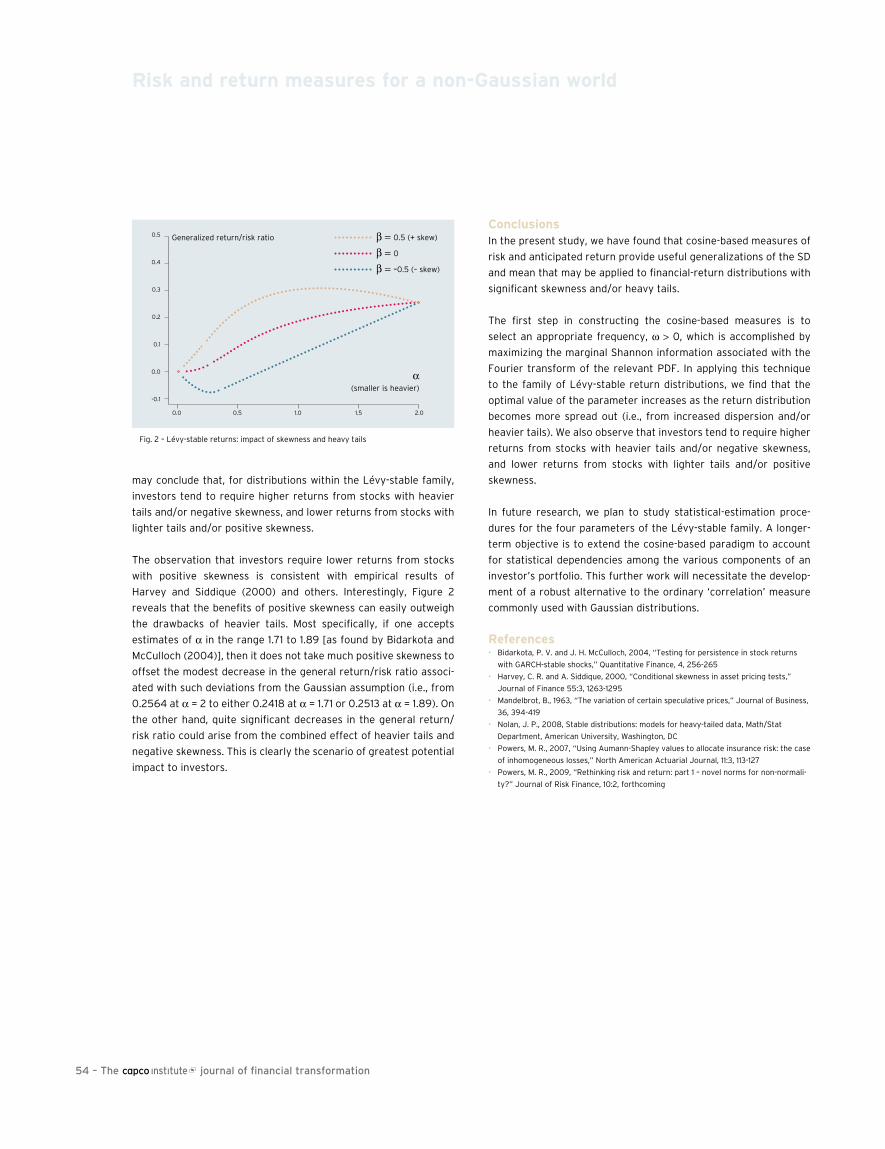
54 – The journal of financial transformation
may conclude that, for distributions within the Lévy-stable family,
investors tend to require higher returns from stocks with heavier
tails and/or negative skewness, and lower returns from stocks with
lighter tails and/or positive skewness.
The observation that investors require lower returns from stocks
with positive skewness is consistent with empirical results of
Harvey and Siddique (2000) and others. Interestingly, Figure 2
reveals that the benefits of positive skewness can easily outweigh
the drawbacks of heavier tails. Most specifically, if one accepts
estimates of α in the range 1.71 to 1.89 [as found by Bidarkota and
McCulloch (2004)], then it does not take much positive skewness to
offset the modest decrease in the general return/risk ratio associ-
ated with such deviations from the Gaussian assumption (i.e., from
0.2564 at α = 2 to either 0.2418 at α = 1.71 or 0.2513 at α = 1.89). On
the other hand, quite significant decreases in the general return/
risk ratio could arise from the combined effect of heavier tails and
negative skewness. This is clearly the scenario of greatest potential
impact to investors.
conclusionsIn the present study, we have found that cosine-based measures of
risk and anticipated return provide useful generalizations of the SD
and mean that may be applied to financial-return distributions with
significant skewness and/or heavy tails.
The first step in constructing the cosine-based measures is to
select an appropriate frequency, ω > 0, which is accomplished by
maximizing the marginal Shannon information associated with the
Fourier transform of the relevant PDF. In applying this technique
to the family of Lévy-stable return distributions, we find that the
optimal value of the parameter increases as the return distribution
becomes more spread out (i.e., from increased dispersion and/or
heavier tails). We also observe that investors tend to require higher
returns from stocks with heavier tails and/or negative skewness,
and lower returns from stocks with lighter tails and/or positive
skewness.
In future research, we plan to study statistical-estimation proce-
dures for the four parameters of the Lévy-stable family. A longer-
term objective is to extend the cosine-based paradigm to account
for statistical dependencies among the various components of an
investor’s portfolio. This further work will necessitate the develop-
ment of a robust alternative to the ordinary ‘correlation’ measure
commonly used with Gaussian distributions.
references• Bidarkota, P. V. and J. H. McCulloch, 2004, “Testing for persistence in stock returns
with GARCH-stable shocks,” Quantitative Finance, 4, 256-265
• Harvey, C. R. and A. Siddique, 2000, “Conditional skewness in asset pricing tests,”
Journal of Finance 55:3, 1263-1295
• Mandelbrot, B., 1963, “The variation of certain speculative prices,” Journal of Business,
36, 394-419
• Nolan, J. P., 2008, Stable distributions: models for heavy-tailed data, Math/Stat
Department, American University, Washington, DC
• Powers, M. R., 2007, “Using Aumann-Shapley values to allocate insurance risk: the case
of inhomogeneous losses,” North American Actuarial Journal, 11:3, 113-127
• Powers, M. R., 2009, “Rethinking risk and return: part 1 – novel norms for non-normali-
ty?” Journal of Risk Finance, 10:2, forthcoming
risk and return measures for a non-Gaussian world
Fig. 2 – Lévy-stable returns: impact of skewness and heavy tails
Generalized return/risk ratio
α(smaller is heavier)
0.5
0.4
0.3
0.2
0.1
0.0
-0.1
0.0 0.5 1.0 1.5 2.0
β = 0.5 (+ skew)
β = 0β = –0.5 (– skew)

55
AbstractIs there a short- to medium-term linkage between macroeco-
nomic and exchange rate volatility? This paper provides a clear-cut
answer to the above question, pointing to significant linkages and
trade-offs between macroeconomic and exchange rate volatility,
particularly involving output volatility. Evidence of bidirectional
causality is also found, with macroeconomic volatility showing a
stronger causal power than exchange rate volatility. Many tasks in
finance, such as option pricing, risk analysis, and portfolio alloca-
tion, rely on the availability of good forecasting models. The paper
points to new directions for the construction of improved medium-
term volatility models.
Medium-term macroeconomic determinants of exchange rate volatility
claudio MoranaDipartimento di Scienze Economiche e Metodi
Quantitativi, Università del Piemonte Orientale, Novara, and International Centre for Economic
Research (ICER, Torino)1
Part 1
1 This paper was presented at the 48th Riunione Annuale della Societa’ Italiana degli
Economisti, Turin, 26-27 October 2007. Funding from MIUR (PRIN project 2005) for
financial support is also gratefully acknowledged.

56
As pointed out by recent contributions to the literature, macro-
economic volatility does not seem to be an important source of
exchange rates volatility for G-7 countries. In fact, little evidence
of exchange rate regime dependence has been found in macro-
economic volatility. For example, unlike exchange rates volatility,
macroeconomic volatility does not tend to be higher in floating rate
regimes than in fixed rates ones. Moreover, little evidence of volatil-
ity conservation has also been found. Apart from output volatility,
no trade-offs between macroeconomic and exchange rates volatil-
ity have been found, suggesting that fixing exchange rates may not
lead to higher macroeconomic volatility in general: excess volatility
simply disappears [Flood and Rose (1995, 1997)]2.
The above findings are not, however, inconsistent with second
moments implications of fundamental models of exchange rate
determination, predicting a linkage between exchange rate and
macroeconomic volatility, for two main reasons. Firstly, once sticky
prices are allowed for, only a weak response of macroeconomic
variables to changes in exchange rate regimes and volatility can be
expected in the short- to medium-term [Duarte (2003)]. Secondly,
other determinants than macroeconomic fundamentals may be
important for exchange rate volatility in the short- to medium-term,
such as excessive speculation [Flood and Rose (1999)], heteroge-
neous agents [Muller et. al. (1997)], overshooting effects related
to information problems [Faust and Rogers (2003)], and informa-
tion flows [Andersen and Bollerslev (1997)], which are, moreover,
responsible for the strong persistence of volatility shocks3.
Unlike from the descriptive analysis carried out in Flood and Rose
(1995, 1997), in this paper accurate modeling of the persistence
properties of the data has been carried out in the framework of a
new fractionally integrated factor vector autoregressive (FI-F-VAR)
model. This latter model allows us to investigate linkages across
variables and countries involving both common deterministic and
stochastic components, consistent with recent findings in the
literature pointing to the presence of both structural change and
stationary long memory in the volatility of financial asset returns
and macroeconomic variables4. Hence, both long-term and medium-
term relationships can be investigated in the current framework,
controlling for short-term dynamic linkages as well. Furthermore,
conditioning is made relative to a very large information set since
the analysis is carried out considering the entire G-7 macroeco-
nomic structure jointly, allowing therefore for a fine control of the
interrelations occurring across countries, currencies, and macro-
economic factors.
The findings of the paper are clear-cut, pointing to significant short-
to medium-term linkages and trade-offs between macroeconomic
and exchange rate volatility, particularly involving output volatility.
Moreover, evidence of bidirectional causality has been found, with
macroeconomic volatility showing a stronger causal power than
exchange rate volatility. Hence, while factors other than macroeco-
nomic fundamentals may be important determinants of exchange
rates volatility in the short- to medium-term, neglecting the impact
of macroeconomic volatility may be inappropriate.
Disposing of accurate models for volatility dynamics is important
under different points of view. In fact, in addition to the understand-
ing of the causes of financial assets volatility, volatility forecasting
also depends on the availability of a good volatility model. Important
tasks in finance, such as option pricing, risk measurement, in the
context of Value at Risk (VaR) models, and portfolio allocation
models, built on the basis of forecasts of returns, variances, and
covariances, do rely on good forecasting models.
The results of the study do point to new directions for the construc-
tion of improved short- to medium-term volatility models. From a
medium-term perspective, forecasting models conditioned to an
information set containing not only their own historical volatilities
but also the history of key macroeconomic volatility series may lead
to more accurate predictions of the overall level of future volatility.
Insofar as feedback effects between macroeconomic and financial
markets volatility can be found, multi-period predictions could also
benefit from a multivariate framework, where interactions between
the involved variables may be fully accounted for. The multivariate
model proposed in this paper does provide a viable and effective
framework suited to the task.
Econometric methodologyConsider the following fractionally integrated factor vector autore-
gressive (FI-F-VAR) model:
xt = Λμμt + Λƒƒt + C(L)(xt-1 – Λμμt-1) + vt (1)
D(L)ƒt = ηt , (2)
where (xt – Λμμt) is a n-variate vector of stationary long memory
processes (0 < di < 0.5, i=1,···,n) [Baillie (1996)], ƒt is an r-variate
vector of stationary long memory factors, μt is an m-variate vector
of common break processes, vt is an n-variate vector of zero mean
idiosyncratic i.i.d. shocks, ηt is an r-variate vector of common zero
mean i.i.d. shocks, E[ηtvis] = 0 all i,t,s, Λƒ and Λμ are n×r and n×m
matrices of loadings, respectively, C(L) is a finite order matrix of
polynomials in the lag operator with all the roots outside the unit
circle, i.e., C(L) = C1L + C2L2 + ··· + Cp(Lp), Ci i=1,···, is a square matrix
of coefficients of order n, and D(L) = diag(1-L)d1, (1-L)d2,···, (1-L)dr is
a diagonal matrix in the polynomial operator of order r. The frac-
tional differencing parameters di, as well as the μt and ƒt factors,
are assumed to be known, although they need to be estimated.
2 Similarly, Baxter and Stockman (1989) had previously found little evidence that
macroeconomic volatility or trade flows are influenced by exchange rate regimes.
Differently, Hutchinson and Walsh (1992) and Bayoumi and Eichengreen (1994) have
found evidence consistent with the insulation properties of a flexible exchange rate
regime, while both Arize et al. (2000) and Rose (2000) have found evidence of sig-
nificant negative, yet small, effects of exchange rate volatility on trade flows.
3 According to Muller et al. (1997), the interaction in the market of agents with dif-
ferent time horizon leads to long memory in exchange rates volatility. Differently,
Andersen and Bollerslev (1997) explain long memory in exchange rates volatility as
the consequence of the aggregation of a large number of news information arrival
processes.
4 See for instance Granger and Hyung (1999) for structural breaks in the volatility of
financial asset returns; Baillie et al. (1996) and Andersen et al. (1997) for long mem-
ory; Lobato and Savin (1998), Morana and Beltratti (2004), and Baillie and Morana
(2007) for both features. For structural breaks and long memory in macroeconomic
volatility see Beltratti and Morana (2006).
Medium-term macroeconomic determinants of exchange rate volatility
57
However, this is not going to affect the asymptotic properties of the
estimator, since consistent estimation techniques are available for
all the parameters and unobserved components.
The reduced fractional Var formBy taking into account the binomial expansion in equation (2)5,
and substituting into equation (1), the infinite order vector autore-
gressive representation for the factors ƒt and the series xt can be
rewritten as:
where D(L) = I-Φ(L), Φ(L) = Φ0L0 + Φ1L1 + Φ2L2 + ··· + Φi, i=1,···, is a
diagonal matrix of coefficients of dimension r,
with variance covariance matrix
where E[ηtη’t] = ∑η and E[vtv’t] = ∑v.
EstimationThe estimation problem may be written as follows: min T-1∑t=1→T
ε’x,tεx,t, where εx,t = [I – C(L)L] [xt – Λμμt] [ΛƒΦ(L)L]ƒt. Yet, since
the infinite order representation cannot be handled in estimation,
truncation to a suitable large lag for the polynomial matrix Φ(L) is
required. Hence, Φ(L) = ∑j=0→p ΦjLj. This model can be understood
as a generalization of the (static) factor VAR model proposed by
Stock and Watson (2005), allowing for both deterministic and long-
memory stochastic factors, and can be estimated by following an
iterative process [See Morana (2008) for estimation details and
Morana (2007a) for supporting Monte Carlo evidence. See also
Morana (2008) for details concerning the identification of the com-
mon and idiosyncratic shocks].
Data and modeling issuesInstead of considering Italy, Germany, and France as separate coun-
tries, the Euro Area-12 aggregate data have been employed in the
paper. This allows us to focus on the most recent float period (1980-
2006), which has been almost entirely neglected in the literature so
far. Monthly time series data for the five countries involved — the
U.S., Japan, the Euro-12 area, the U.K., and Canada — over the period
1980:1-2006:6, have been employed. In addition to the four nomi-
nal exchange rate variables against the U.S.$ — the €/U.S.$ rate,
the ¥/U.S.$ rate, the GBP£/U.S.$ rate, and the Canadian $/U.S.$
rate — four macroeconomic variables for each country have also
been considered, the real industrial production growth rate, the
CPI inflation rate, the nominal money growth rate, and the nominal
short-term interest rates6,7.
Monthly (log) volatility proxies for the above variables have been
constructed as the (log) absolute value of the innovations of the
various series, obtained from the estimation of a standard VAR
model for the 24 variables in the dataset, with lag length set to two
lags on the basis of misspecification tests and the AIC criterion.
Although this yields noisy volatility proxies, the use of an effective
noise filtering procedure grants reliability to the results obtained
in the study. The selection of the dataset follows the monetarist
models of exchange rate determination, from which the following
reduced form exchange rate equation can derived: e = (ms – ms*) –
ф(y-y*) + α(i-i*) + ф(π-π*), stating that the log level of the nominal
exchange rate (e) is determined by differentials in the log money
supplies (ms), log real outputs (y), nominal interest rates (i), and
inflation rates (π) between the domestic and foreign (starred vari-
ables) countries8. Hence, a general long-term reduced form equa-
tion may be written as et = z’tδ + εt, where the vector zt contains
the macroeconomic fundamentals and εt is a zero mean stochastic
disturbance term capturing non-fundamental determinants, for
instance related to speculative behavior in the exchange rate mar-
ket. Hence, by moving to second moments, assuming orthogonal
fundamentals and non-fundamental determinants, it follows s2e,t =
s2z,t’δ2 + s2ε,t, pointing to a linkage between exchange rate (s2
e,t),
fundamental (s2z,t, macroeconomic) and non-fundamental uncondi-
tional volatility (s2ε,t)9.
Consistent with general findings in the literature and the results
of this study, both exchange rate and macroeconomic volatility
is modeled as a long memory process (I(d), 0<d<0.5), subject to
structural change. Hence, following Morana (2007a) for the generic
ith exchange rate volatility process one has s2i,t = bt + Pt + NPt,
where bt is the deterministic break process (time-varying uncon-
ditional variance) of the series — i.e., the permanent or long-term
component — expected to be related to fundamentals — i.e., [bt =
ƒ(s2z,t’δ2), Pt is the persistent (long memory, I(d)] or medium-term
component — expected to be related to the non fundamental vola-
tility component or only weakly related to fundamentals — i.e., Pt =
(ƒ(s2ε,t), in the light of the explanations provided for long memory
in volatility [Andersen and Bollerslev (1997), Muller et al. (1997)] —
and NPt is the non-persistent or noise component (I(0)), with E[Pt]
= 0 and E[NPt] = 0.
5 (1-L)d = ∑j=1→∞ ρjLj, ρj = ∑k=0→∞ Γ(j-d)/ [Γ(j+1) Γ(-d)], where Γ(·) is the gamma function.
6 Nominal money balances are given by M2 for the U.S., M2+CD for Japan, M3 for the
Euro Area and Canada, and M4 for the U.K. The aggregates employed are the one
usually employed to measure broad money in each of the countries investigated. On
the other hand, the short-term rate refers to three-month government bills. The use
of broad money is justified by country homogeneity, since, as far as Japan is con-
cerned, in the view of the near liquidity trap experienced by this latter countries over
the 1990s, the use of narrow money would have been problematic.
7 Synthetic Euro Area data are employed in this study. The author is grateful to the
ECB, Monetary Policy Strategy Division, for data provision.
8 In particular, if α<0, β>0, |β|>|α| the Frenkel real interest differential model is
obtained; if α>0, β=0 the flexible price monetarist model is obtained; if α=0, β>0
the flexible price with hyperinflation monetarist model is obtained; if α<0, β=0 the
Dornbusch-sticky price monetarist model is obtained. Finally, assuming β=0, and
including in the equation the equilibrium real exchange rate, the equilibrium model is
obtained. See Taylor (1995) for additional details.
9 A similar relationship can be easily derived for the conditional variance.
Medium-term macroeconomic determinants of exchange rate volatility
ƒt
xt - Λμμt
Φ(L) 0
ΛƒΦ(L) C(L)
εƒt
εxt
ƒt-1
xt-1 - Λμμt-1= = , (3)
εƒt
εxt
I
Λƒ
0
vt= ηt +
Σ’η
Λƒ Σ’η
Σ’η Λ’ƒ
Λƒ Σ’η Λ’ƒ + ΣvE[εtε’t] = Σε = ,

58 – The journal of financial transformation
Linkages among volatility series can then concern either the long-
term or break process component bt or the medium-term or long
memory component Pt, or both. The FI-F-VAR model allows us to
account for both kinds of linkages, controlling for short-term dynam-
ic linkages as well. Moreover, conditioning is made relative to a very
large information set, i.e., the entire G-7 macroeconomic structure,
which therefore allows us to control the interrelations occurring
across countries, currencies, and macroeconomic factors.
Persistence propertiesIn the light of recent results in the literature pointing to the presence
of both long memory and structural change in the volatility of finan-
cial assets, as well as in macroeconomic variables, the persistence
properties of the data have been assessed by means of structural
break tests and semiparametric estimators of the fractional differ-
encing parameter. Structural change analysis has been carried out
by means of the Dolado et al. (2004) test, modified to account for a
general and unknown structural break process. Dolado et al. (2004)
have proposed a Dickey-Fuller type of test for the null of I(d) behav-
ior, 0<d≤1, against the alternative of trend stationarity I(0), with or
without structural breaks. A simple generalization of the model,
allowing for a general nonlinear deterministic break process, can be
obtained by specifying the trend function according to the Gallant
(1984) flexible functional, as in Enders and Lee (2004):
ABNL(t) = μ0 + β0
t + ∑k=1→pβs,ksin(2πkt/T) + βc,kcos(2πkt/T) allow-
ing for a suitable order (p) for the trigonometric expansion. The
process under H1 is then Δdyt = ΔdABNL(t) – ϕAB
NL(t-1)yt-1 + ϕyt-1
+ ∑j=1→sΔdyt-j + vt, with vt ~ iid(0, sv2). The null hypothesis of I(d)
implies ф = 0, while the alternative of I(0) stationarity plus structur-
al change implies ф < 0. Critical values can be easily computed, case
by case, by means of the parametric bootstrap [Poskitt (2005)].
Monte Carlo evidence supporting the use of the above adaptive
approach for structural break estimation can be found in Cassola
and Morana (2006), where details concerning the selection of the
order of the trigonometric expansion can also be found.
Moreover, since the computed log volatility series are likely to be
characterized by observational noise, the fractional differencing
parameter employed in the test has been estimated by means of
the Sun and Phillips (2003) non-linear log periodogram estimator,
which does not suffer from the downward bias affecting standard
semiparametric estimators in this latter situation.
structural break and long memory analysisAs shown in Figure 1, Panel A, there is strong evidence of struc-
tural change in the volatility series investigated, since the null of
pure long memory against the alternative of structural change is
strongly rejected (at the 1% significance level) for all the series,
Medium-term macroeconomic determinants of exchange rate volatility
Panel A – Dolado et al. (2004) structural break tests
gUS -4.381* πUS -4.447* sUS -1.132 mUS -4.409*
gEA -4.358* πEA -1.849 sEA -3.447* mEA -6.128* eEA -5.688*
gJA -4.598* πJA -4.079* sJA -4.352* mJA -4.792* mJA -4.996*
gCA -4.980* πCA -5.211* sCA -4.818* mCA -4.087* mCA -3.655*
gUK -5.152* πUK -4.513* sUK -4.248* mUK -3.849* mUK -4.761*
Panel B – fractional differencing parameter estimation
gUS 0.346(0.106)
[15]
πUS 0.346(0.061)
[26]
sUS 0.320(0.111)[15]
mUS 0.310(0.073)
[23]
gEA 0.363(0.081)
[19]
πEA 0.303(0.090)
[19]
sEA 0.303(0.067)
[26]
mEA 0.309(0.091)
[19]
eEA 0.325(0.080)
[21]
gJA 0.338(0.078)
[23]
πJA 0.328(0.074)
[22]
sJA 0.274(0.076)
[24]
mJA 0.249(0.086)
[23]
mJA 0.277(0.106)
[17]
gCA 0.356(0.047)
[33]
πCA 0.310(0.106)
[16]
sCA 0.311(0.088)
[19]
mCA 0.284(0.056)
[32]
mCA 0.300(0.076)
[23]
gUK 0.304(0.095)
[18]
πUK 0.299(0.099)
[18]
sUK 0.353(0.080)
[20]
mUK 0.249(0.118)
[17]
mUK 0.304(0.070)
[25]
Figure 1 – Persistence analysis
Panel A reports the value of the Dolado et al. (2004) test. * denotes significance at the 1% level. In Panel B the estimated fractional differencing parameters obtained using the Sun
and Phillips (2003) non linear log periodogram estimator, with standard errors ((·)) and selected ordinates ([·]), are reported. The log volatility series investigated are real output
growth rates (g), inflation rates (π), short-term nominal interest rates (s), nominal money growth rates (m), and nominal exchange rates returns for the euro, the Japanese yen, the
British pound, and the Canadian dollar against the U.S. dollar (e).

59
apart from the Euro Area CPI inflation rate and the U.S. short-
term rate series10. Moreover, as shown in Panel B, the Sun and
Phillips (2003) non-linear log periodogram estimation carried out
on the break-free processes points to a moderate degree of long
memory characterizing the break-free processes, ranging from
0.249(0.086) to 0.363(0.081), and to large inverse long-run signal
to noise ratios, ranging from 16.960(5.162) to 30.113(7.236). Since in
none of the cases the Robinson and Yajima (2001) test allows us to
reject the null of equality of the fractional differencing parameter, a
single value for the fractional differencing parameter has then been
obtained by averaging the twenty four available estimates, yielding
a point estimate of 0.311(0.084). Similarly, the average value of the
inverse long-run signal to noise ratio is equal to 22.245(5.256). In
the light of the above results, the estimated candidate break pro-
cesses have then been retained as non-spurious for all the series.
In fact, in none of the cases the removal of the estimated break
process from the actual series has led to an antipersistent process,
i.e., to an integrated process I(d) with d<0 [Granger and Hyung
(2004)]12.
Yet, given the size of the inverse long-run signal to noise ratios, fil-
tering of the volatility components is required before further analy-
sis is carried out on the break-free series. In the paper the approach
of Morana (2007b) has been implemented. The approach is based
on flexible least squares estimation and it has been found to per-
form very satisfactorily by Monte Carlo analysis, independently
of the actual characteristics of the noisy stochastic process, i.e.,
deterministic versus stochastic persistence and long versus short
memory, also when the inverse signal to noise ratio is very large13.
The fI-f-VAr modelThe minimum dimension of the FI-F-VAR model in the current data
framework is twenty four equations, corresponding to the log volatili-
ty series for the twenty macroeconomic series and the four exchange
rate series. Additional equations would refer to the common long
memory factors, whose existence has however to be determined
through principal components analysis (PCA), consistent with the
first step required for the estimation of the FI-F-VAR model.
In order to investigate medium-term linkages between macroeco-
nomic and exchange rates volatility, the two-country specification
implied by standard economic theories of bilateral exchange rates
determination has been employed. Hence, linkages between macro-
economic and exchange rates volatility have been investigated with
reference to a single bilateral exchange rate at the time and the
macroeconomic variables of the involved countries. Moreover, in
order to focus on short- to medium-term linkages only, the analysis
has been carried out on the break-free processes obtained in the
previous section.
Principal components analysisAs shown in Figure A1 in the Appendix, principal components
analysis points to interesting linkages involving macroeconomic
and exchange rate volatility in the medium term. In fact, in all
of the cases seven principal components out of nine are neces-
sary to explain about 90% of total variability, with the bulk of
exchange rates volatility (58% to 83%) explained by the first five
components. Similarly, the proportion of macroeconomic volatil-
ity explained by the first five components is in the range 50% to
95% for output volatility, 70% to 82% for inflation volatility, 62%
to 85% for interest rate volatility, and 61% to 93% for money
growth volatility. Furthermore, other linkages can be noted across
currencies. For example, an interesting linkage involving output
growth and exchange rate volatility for the €/U.S.$ and the ¥/U.S.$
exchange rates can be found. In fact, in both cases the dominant
component for exchange rates volatility is also dominant for
output growth volatility (49% for eEA and 35% and 25% for gUS
and, respectively; 39% for eJA and 46% and 12% for gUS and gJA,
respectively). In addition, while interest rate volatility is related
to exchange rates volatility for both currencies, money growth
volatility is related to exchange rates volatility only for the €/U.S.$
exchange rate. For inflation volatility the linkage is only relevant
for the ¥/U.S.$ exchange rate. On the other hand, for the Canadian
$/U.S.$ exchange rate the linkage involves all the macroeconomic
volatility series. Finally, for the £/U.S.$ exchange rate the linkage
is weaker than for the other currencies, being non-negligible only
concerning inflation volatility.
By assessing the proportion of variance explained by the same
principal component, but with impact of opposite sign, for the vari-
ous break-free series some evidence of a medium-term trade-off
10 Following the Monte Carlo results reported in Cassola and Morana (2006), a fourth
order trigonometric expansion has been employed for the computation of the struc-
tural break tests.
11 The minimum p-value for the Robinson and Yajima (2002) equality test is equal to
0.423, which is very far apart from any usual significance value for the rejection of a
simple or joint null hypothesis.
12 In order to assess the robustness of the results, the break tests have been repeated
considering trigonometric expansions of the first, second, and third order, allowing
the fractional differencing parameter to take three different values, d=0.2, 0.3, 0.4
in each case. The results point to the robustness of the structural break tests to both
the order of the trigonometric expansion and the selection of the fractional differenc-
ing parameter.
13 All the empirical findings reported in the paper are robust to the noise filtering pro-
cedure implemented. Details are not reported for reasons of space, but are available
upon request from the author.
Medium-term macroeconomic determinants of exchange rate volatility
€/U.s.$ ¥/U.s.$ £/Us$ cA$/U.s.$
gUS 0.70 0.48 0.70 0.63
gi 0.50 0.22 0.87 0.51
πUS 0.83 0.47 0.31 0.41
πi 0.53 0.68 0.60 0.86
sUS 0.40 0.49 0.17 0.51
si 0.34 0.49 0.36 0.29
mUS 0.47 0.82 0.20 0.54
mi 0.77 0.70 0.80 0.73
The table reports the proportion of variance for each macroeconomic volatility
variable involved in the trade-off. Hence, i=EA for the €/U.S.$, JA for the ¥/US$, U.K.
for the £/U.S.$, CA for the CA$/U.S.$. The variables investigated are log volatilities
for real output growth rates (g), inflation rates (π), short-term nominal interest rates
(s), nominal money growth rates (m). Columns correspond to the four exchange
rates.
Figure 2 – Medium-term trade-off analysis

60 – The journal of financial transformation
between exchange rate and macroeconomic volatility can also be
found (Figure 2). The following findings are noteworthy. Firstly, on
average, the variables which are more affected by the trade-off are
output growth (58%), inflation (59%), and money growth (63%)
volatility. On the other hand, short-term rate volatility (39%) is the
variable for which the trade-off is weakest. Interesting differences
can also be found across exchange rates on the same horizon. For
example, the trade-off is in general strongest for output growth
for the U.K and for money growth for the U.S. Moreover, for the
latter two variables the trade-off is weakest for Japan. In addition,
for inflation and the short-term rate the trade-off is strongest for
Canada and the U.S./Japan, respectively, and weakest for the U.K.
In general, the U.S is a country strongly affected by the trade-off,
followed by the U.K. and the Euro Area, while Canada and Japan fall
in an intermediate ranking.
Granger causality analysisSince principal components analysis cannot establish any causal
direction in the linkage between macroeconomic and exchange rate
volatility, Granger causality analysis has been carried out following
Chen (2006) and Bauer and Maynard (2006), i.e., by means of stan-
dard VAR analysis carried out using the pre-filtered series for the
long memory effects and by means of VAR analysis carried out on
the actual series, exploiting the surplus lag principle, respectively.
Hence, with reference to the sth variable of interest, the following
equations have been estimated: y*s,t = α + ∑j=1→m βjy*s,t-j + ∑j=1→m
x-t-jγ’j + εt; and y*s,t = α + ∑j=1→m+1 βjy*s,t-j + ∑j=1→m+1 x
-t-jγ’j + εt, with
m = 1, ..., 12, where the vector of forcing variables for the variable of
interest y*s,t is given by x-t, which is the vector xt excluding the vari-
able of interest y*s,t. For example, xt = [x-t y*s,t]’. y*t is the vector
of break-free long memory prefiltered variables [(1-L)d (yi,t – bpi,t),
i=1,...,24)] in the first case [Chen (2006) test] and the vector of
break-free actual variables [(yi,t – bpi,t), i=1,...,24)] in the second case
[Bauer and Maynard (2006) test]. The auxilary VAR regressions
have been estimated considering an increasing number of lags m,
i.e., m = 1, ..., 12, and the null of Granger non-causality from appropri-
ate subsets of variables in x-t to variable y*s,t has been tested using
the Wald test, for all the different lag orders.
A summary of the results of the Granger causality analysis are
reported in Figure 3. As is shown in the table, evidence of bidirec-
tional causality can be found at the 1% significance level, indepen-
dently of the approach implemented. In particular, the findings are
similar across countries, also pointing to a similar causal power of
macroeconomic and exchange rate volatility. In general, output and
inflation volatility tend to have a stronger impact on exchange rate
volatility than interest rate and money growth volatility. The impact
of exchange rate volatility on macroeconomic volatility tends to be
homogeneous across variables.
forecast error variance decompositionOn the basis of the results of the principal components analysis
and the relatively high number of factors necessary to explain the
bulk of total variance for the break-free variables, no common long
memory factors have been added to the model. Hence, the final
specification of the FI-F-VAR model is composed of just the twenty-
four equations corresponding to the log volatilities for twenty-four
variables in the dataset. The model has then been estimated with-
out long memory prefiltering, exploiting the (truncated) infinite
order VAR representation of the VARFIMA structure of the model,
including seven common deterministic break processes14.
Thick estimation [Granger and Jeon (2004)] has been implemented
by optimally selecting the lag order by information criteria and
14 The selection is consistent with the results of the principal components analysis car-
ried out on the break processes for the 24 variables involved, pointing that seven
common break processes (factors) are necessary to account for about 95% of total
variance. Detailed results are not reported, but are available upon request from the
author.
Medium-term macroeconomic determinants of exchange rate volatility
chen tests
gUS 0.001 πUS0.094 sUS 0.000 mUS 0.000 g π s m
gEA 0.035 πEA0.000 sEA 0.012 mEA 0.007 eEA 0.003 0.010 0.036 0.100
gJA 0.044 πJA0.001 sJA 0.000 mJA 0.027 mJA 0.099 0.012 0.020 0.018
gCA 0.011 πCA0.001 sCA 0.078 mCA 0.000 mCA 0.000 0.001 0.000 0.000
gUK 0.000 πUK0.022 sUK 0.002 mUK 0.007 mUK 0.005 0.004 0.000 0.007
Bauer-Maynard tests
gUS 0.004 πUS0.017 sUS 0.000 mUS 0.000 g π s m
gEA 0.002 πEA0.000 sEA 0.033 mEA 0.019 eEA 0.002 0.001 0.079 0.016
gJA 0.768 πJA0.020 sJA 0.017 mJA 0.010 mJA 0.018 0.001 0.159 0.000
gCA 0.029 πCA0.011 sCA 0.033 mCA 0.002 mCA 0.000 0.152 0.001 0.050
gUK 0.000 πUK0.001 sUK 0.020 mUK 0.012 mUK 0.014 0.051 0.001 0.003
Figure 3 – Granger causality tests
The table reports the minimum p-value for the causality tests. Figures for the macroeconomic variables refer to the null of no Granger causality from exchange rate volatility to
macroeconomic volatility. Figures for the exchange rate series refer to the null of no Granger causality from macroeconomic volatility to exchange rate volatility, distinguishing
among categories of macroeconomic variables. The variable investigated are log volatilities for real output growth rates (g), inflation rates (π), short-term nominal interest rates (s),
nominal money growth rates (m), and bilateral nominal exchange rates returns for the €, the ¥, the £, and the Canadian $ against the U.S.$ (e).
61
then allowing for two additional specifications of higher and lower
lag orders. According to the Akaike and Hannan-Quin information
criteria, two lags have been selected, while according to the Bayes
information criterion, just one lag could be selected. Hence, median
estimates have been obtained by considering lag orders up to the
third order. Monte Carlo replications have been set to 1000 for each
case, considering two different orders for the variables, i.e., the
volatility series have been ordered as output, inflation, short-term
rate, money growth, and exchange rates, with countries selected
as the U.S., Euro Area, Japan, the U.K. and Canada in the first case,
and inverting the previous order in the second case. The median
estimates have therefore been obtained from cross-sectional dis-
tributions counting 6000 units.
As shown in Figure A2 in the Appendix, the results of the fore-
cast error variance decomposition (FEVD) analysis are clear-cut,
pointing to mostly idiosyncratic long memory dynamics for all
the variables. In fact, the own shock explains the bulk of volatil-
ity fluctuations for all the variables at all the horizons, with the
contribution of the other shocks increasing as the forecast horizon
increases. For instance, on average, output volatility shocks explain
between 77% and 85% of output volatility variance at the selected
horizons. Similarly, inflation volatility shocks explain between 75%
and 85% of inflation volatility variance. On the other hand, figures
for the short-term rate and the money growth volatility are in the
range 82% to 88% and 82% to 87%, respectively. Moreover, for
the exchange rates figures are in the range 77% to 85%. In all the
cases it is always the own volatility shock that explains the bulk of
variability for the log volatility series. Finally, while some contribu-
tion to the explanation of macroeconomic volatility is provided by
the exchange rate shocks, a much stronger role seems to be played
by the macroeconomic shocks. In fact, on average the exchange
rate volatility shocks explain only about 5% of macroeconomic
volatility variance at all the forecasting horizons considered, while
the average contribution of macroeconomic volatility shocks to
exchange rate volatility variance is about 20%. Hence, a stronger
short- to medium-term causality linkage from macroeconomic
volatility to exchange rate volatility than the other way around is
revealed by the FEVD analysis.
conclusionAs pointed out by the empirical analysis, significant short- to
medium-term linkages and trade-offs between macroeconomic and
exchange rate volatility can be found for the G-7 countries, particu-
larly involving output, inflation, and money growth volatility. While
these linkages show bidirectional causality, macroeconomic vola-
tility does seem to be a stronger driving force for exchange rate
volatility than the other way around. The seminal views of Friedman
(1953) on the case for flexible exchange rates seem to find support,
from a medium-term perspective, with interesting implications for
financial analysis. Since macroeconomic stability may be important
to reduce excess exchange rates volatility, monitoring the making
of economic policy may be relevant for predicting future regimes
of low/high volatility, which may persist over time. Moreover, as
systemic volatility cannot be eliminated, even in fixed exchange
rate regimes, feedback effects should also be taken into account.
Hence, while other factors than macroeconomic fundamentals may
be important determinants of exchange rates volatility in the short-
to medium-term, neglecting the impact of macroeconomic volatility
may however be inappropriate. The finding is fully consistent with
additional evidence available for the U.S. stock market [Beltratti
and Morana (2006), Engle and Rangel (2008)], pointing therefore
to a robust linkage between macroeconomic and financial markets
volatility in general.
Many tasks in finance, such as option pricing, risk measurement,
and optimal portfolio allocation do rely on good volatility forecast-
ing models. The results of this study point to new directions for the
construction of improved short- to medium-term volatility models.
With a medium-term perspective, forecasting models conditioned
to an information set containing not only their own historic volatil-
ity but also the history of key macroeconomic volatility series may
lead to more accurate predictions of the overall level of future
volatility [Engle and Rangel (2008)]. Furthermore, insofar as
feedback effects between macroeconomic and financial markets
volatility can be found, multi-period predictions could benefit from
a multivariate framework, where interactions between the involved
variables may be fully accounted for. The multivariate model pro-
posed in this paper does provide a viable and effective framework
suited to the task.
Some applications to conditional portfolio allocation, coherent with
the results of the study, can also be mentioned. For example, both
the conditional approaches of Brandt and Santa-Clara (2003) and
Brandt et al. (2004) are directly related to the use of macroeco-
nomic information for the estimation and prediction of optimal
portfolio weights. More recently, Morana (2007c), still in the
framework of conditional portfolio models, has proposed a sim-
pler, yet effective, alternative approach to exploit macroeconomic
information for ex-post predictions of the optimal portfolio weights,
which are derived without explicit conditioning to macroeconomic
information. While the advantages of the multivariate structural
volatility modeling, discussed above, over standard univariate
methodologies are clear-cut in principle, additional work is needed
to provide complementary empirical evidence. We leave this issue
for future work.
Medium-term macroeconomic determinants of exchange rate volatility

62 – The journal of financial transformation
references• Andersen, T. G., and T. Bollerslev, 1997, “Heterogeneous information arrivals and
return volatility dynamics: uncovering the long-run in high frequency returns,” Journal
of Finance, 52, 975-1005
• Arize, A., T. Osang, and D. Slottje, 2000, “Exchange rate volatility and foreign trade:
evidence from thirteen LDCs,” Journal of Business and Economic Statistics, 18, 10-17
• Bai, J., 2004, “Estimating cross-section common stochastic trends in nonstationary
panel data,” Journal of Econometrics, 122, 137-38
• Bai, J., 2003, “Inferential theory for factor models of large dimensions,” Econometrica,
71:1, 135-171
• Bai, J., and S. Ng, 2004, “A panic attack on unit roots and cointegration,”
Econometrica, 72:4, 1127-1177
• Baillie, R. T., T. Bollerslev and O. H. Mikkelsen, 1996, “Fractionally integrated genera-
lised autoregressive conditional heteroskedasticity,” Journal of Econometrics, 74, 3-30
• Baillie, R. T., 1996, “Long memory processes and fractional integration in economet-
rics,” Journal of Econometrics, 73, 5-59
• Baillie, R. T., and C. Morana, 2007, “Modeling long memory and structural breaks
in conditional variances: an adaptive FIGARCH approach,” mimeo, Michigan State
University
• Bauer, D., and A. Maynard, 2006, “Robust granger causality test in the VARX frame-
work,” mimeo, University of Toronto
• Baxter, M., and A. Stockman, 1989, “Business cycles and the exchange rate regime,”
Journal of Monetary Economics, 23, 337-400
• Bayoumi, T., and B. Eichengreen, 1994, “Macroeconomic adjustment under Bretton-
Woods and the post-Bretton-Woods float: an impulse response analysis,” Economic
Journal, 104, 813-27
• Beltratti, A., and C. Morana, 2006, “Breaks and persistency: macroeconomic causes of
stock market volatility,” Journal of Econometrics, 131, 151-71
• Bierens, H. J., 2000, “Nonparametric nonlinear cotrending analysis, with an applica-
tion to interest and inflation in the United States,” Journal of Business and Economic
Statistics, 18:3, 323-37
• Brandt, M. W., 1999, “Estimating portfolio and consumption choice: a conditional euler
equations approach,” Journal of Finance, 54, 1609-1646
• Brandt, M. W., and P. Santa-Clara, 2003, “Dynamic portfolio selection by augmenting
the asset space,” mimeo, Duke University
• Cassola, N., and C. Morana, 2006, “Comovements in volatility in the euro money mar-
ket,” European Central Bank Working Paper Series, no. 703
• Chen, W-D., 2006, “Estimating the long memory granger causality effect with a spec-
trum estimator,” Journal of Forecasting, 25, 193-200
• Dolado, J. J., J. Gonzalo, and L. Mayoral, 2004, “A simple test of long memory vs.
structural breaks in the time domain,” Universidad Carlos III de Madrid, mimeo
• Duarte, M., 2003, “Why don’t macroeconomic quantities respond to exchange rate
volatility?” Journal of Monetary Economics, 50, 889-913
• Enders, W., and J. Lee, 2004, “Testing for a unit-root with a non linear fourier func-
tion,” mimeo, University of Alabama
• Engle, R. F., and C. W. J. Granger, 1987, “Co-integration and error correction represen-
tation, estimation, and testing,” Econometrica, 55, 251-76
• Engle, R. F., and J. G. Rangel, 2008, “The spline GARCH model for unconditional volatil-
ity and its global macroeconomic causes,” The Review of Financial Studies
• Faust, J., and J. H. Rogers, 2003, “Monetary policy’s role in exchange rate behavior,”
Journal of Monetary Economics, 50, 1403-1424
• Flood, R. P. and A. K. Rose, 1995, “Fixing exchange rates. A virtual quest for fundamen-
tals,” Journal of Monetary Economics, 36, 3-37
• Flood, R. P. and A. K. Rose, 1999, “Understanding exchange rate volatility without the
contrivance of macroeconomics,” mimeo, University of California, Berkeley
• Friedman, M., 1953, “The case for flexible exchange rates,” in Essays in Positive
Economics, Chicago: University Press
• Gallant, R., 1984, “The fourier flexible form,” American Journal of Agricultural
Economics, 66, 204-08
• Granger, C. W. J., and Y. Jeon, 2004, “Thick modelling,” Economic Modelling, 21, 323-
43
• Granger, C. W. J. and N. Hyung, 2004, “Occasional structural breaks and long memory
with an application to the S&P500 absolute returns,” Journal of Empirical Finance, 11:3,
399-421
• Hutchinson, M., and C. Walsh, 1992, “Empirical evidence on the insulation properties of
fixed and flexible exchange rates: the Japanese experience,” Journal of International
Economics, 34, 269-87
Medium-term macroeconomic determinants of exchange rate volatility
• Lobato I. N. and N.E. Savin, 1998, “Real and spurious long memory properties of stock
market data,” Journal of Business and Economic Statistics, 16:3, 261-68
• Marinucci, D., and P. M., Robinson, 2001, “Semiparametric fractional cointegration
analysis,” Journal of Econometrics, 105, 225-47
• Morana, C., 2008a, A factor vector autoregressive estimation approach for long memo-
ry processes subject to structural breaks, Universita’del Piemonte Orientale, mimeo.
• Morana, C., 2007a, “Multivariate modelling of long memory processes with common
components,” Computational Statistics and Data Analysis, 52, 919-934
• Morana, C., 2007b, “An omnibus noise filter,” mimeo, Università del Piemonte Orientale
• Morana, C., 2007c, “Realized portfolio selection in the euro area,” mimeo, Università
del Piemonte Orientale
• Morana, C., and A. Beltratti, 2004, “Structural change and long range dependence in
volatility of exchange rates: either, neither or both?” Journal of Empirical Finance, 11:5,
629-58
• Muller, U. A., M. M. Dacorogna, R. D. Davé, R. B. Olsen, O.V. Pictet, and J. E. von
Weizsacker, 1997, “Volatilities of different time resolutions – analyzing the dynamics of
market components,” Journal of Empirical Finance, 4, 213-39
• Pesaran, M. H., and Y. Shin, 1998, “Generalised impulse response analysis in linear mul-
tivariate models,” Economics Letters, 58, 17-29
• Poskitt, D. S., 2005, “Properties of the sieve bootstrap for non-invertible and fraction-
ally integrated processes,” mimeo, Monash University
• Robinson, P. M., and Y. Yajima, 2002, “Determination of cointegrating rank in fractional
systems,” Journal of Econometrics, 106:2, 217-41
• Rose, A., 1996, “After the deluge: do fixed exchange rates allow intertemporal volatility
tradeoffs?” International Journal of Finance and Economics, 1, 47-54
• Stock, J. H., and M. W. Watson, 2005, “Implications of dynamic factor models for VAR
analysis, NBER Working Paper, no. 11467
• Sun, Y., and P. C. B. Phillips, 2003, “Non linear log-periodogram regression for per-
turbed fractional processes,” Journal of Econometrics, 115, 355-89
• Taylor, M., 1995, “The economics of exchange rates,” Journal of Economic Literature,
33, 13-47

63
Medium-term macroeconomic determinants of exchange rate volatility
€/U.s.$ Pc1
Pc2
Pc3
Pc4
Pc5
Pc6
Pc7
Pc8
Pc9
All 0.19 0.16 0.15 0.14 0.10 0.08 0.07 0.06 0.05
gUS 0.06 0.35 0.12 0.24 0.02 0.01 0.04 0.05 0.11
gEA 0.19 0.25 0.14 0.07 0.03 0.03 0.21 0.08 0.00
πUS 0.13 0.04 0.40 0.01 0.20 0.08 0.10 0.01 0.04
πEA 0.36 0.04 0.31 0.01 0.08 0.00 0.02 0.05 0.13
sUS 0.29 0.21 0.02 0.07 0.04 0.26 0.04 0.00 0.08
sEA 0.25 0.00 0.18 0.03 0.39 0.00 0.08 0.08 0.00
mUS 0.12 0.03 0.13 0.36 0.02 0.24 0.00 0.09 0.00
mEA 0.26 0.06 0.00 0.36 0.09 0.00 0.12 0.09 0.03
eEA 0.03 0.49 0.02 0.10 0.07 0.14 0.02 0.10 0.04
¥/U.s.$ Pc1
Pc2
Pc3
Pc4
Pc5
Pc6
Pc7
Pc8
Pc9
All 0.18 0.16 0.14 0.13 0.12 0.08 0.07 0.07 0.05
gUS 0.04 0.04 0.46 0.05 0.20 0.15 0.02 0.00 0.06
gJA 0.00 0.52 0.12 0.08 0.01 0.01 0.18 0.00 0.08
πUS 0.12 0.28 0.10 0.20 0.02 0.00 0.03 0.24 0.01
πJA 0.13 0.34 0.01 0.13 0.09 0.09 0.13 0.04 0.04
sUS 0.25 0.00 0.02 0.08 0.42 0.09 0.07 0.00 0.05
sJA 0.35 0.10 0.14 0.00 0.03 0.25 0.10 0.01 0.01
mUS 0.63 0.03 0.03 0.00 0.03 0.02 0.01 0.11 0.14
mJA 0.09 0.10 0.01 0.55 0.00 0.06 0.01 0.17 0.00
eJA 0.01 0.06 0.39 0.10 0.26 0.00 0.08 0.01 0.08
£/U.s.$ Pc1
Pc2
Pc3
Pc4
Pc5
Pc6
Pc7
Pc8
Pc9
All 0.20 0.16 0.14 0.13 0.11 0.09 0.07 0.06 0.05
gUS 0.07 0.20 0.07 0.16 0.00 0.45 0.01 0.03 0.00
gUK 0.00 0.43 0.08 0.21 0.00 0.02 0.23 0.02 0.00
πUS 0.16 0.00 0.01 0.55 0.10 0.00 0.05 0.13 0.01
πUK 0.36 0.11 0.22 0.02 0.01 0.04 0.05 0.12 0.07
sUS 0.60 0.09 0.03 0.02 0.01 0.00 0.00 0.07 0.17
sUK 0.47 0.01 0.03 0.13 0.01 0.13 0.07 0.14 0.02
mUS 0.04 0.56 0.07 0.02 0.03 0.10 0.11 0.00 0.08
mUK 0.03 0.05 0.06 0.08 0.71 0.04 0.01 0.00 0.00
eUK 0.02 0.00 0.72 0.01 0.08 0.02 0.06 0.01 0.08
cA/Us$ Pc1
Pc2
Pc3
Pc4
Pc5
Pc6
Pc7
Pc8
Pc9
All 0.23 0.16 0.14 0.13 0.10 0.09 0.07 0.04 0.04
gUS 0.06 0.10 0.23 0.12 0.44 0.01 0.01 0.04 0.00
gCA 0.13 0.12 0.31 0.00 0.12 0.25 0.00 0.01 0.05
πUS 0.00 0.16 0.28 0.31 0.02 0.12 0.03 0.06 0.00
πCA 0.35 0.22 0.01 0.20 0.00 0.05 0.03 0.05 0.09
sUS 0.44 0.26 0.00 0.02 0.03 0.05 0.02 0.12 0.05
sCA 0.42 0.04 0.18 0.00 0.08 0.05 0.12 0.07 0.04
mUS 0.04 0.36 0.00 0.12 0.09 0.21 0.17 0.00 0.00
mCA 0.17 0.19 0.09 0.35 0.10 0.00 0.00 0.00 0.10
eCA 0.42 0.01 0.12 0.01 0.02 0.10 0.27 0.04 0.01
Figure A1 – Principal components analysis (medium-term), bilateral exchange rates models
The table reports the results of the medium-term principal components (PC) analysis carried out for each exchange rate on the break-free noise-free log-volatility for the relevant
macroeconomic variables, i.e. real output growth rates (g), inflation rates (π), short-term nominal interest rates (s), nominal money growth rates (m), and nominal exchange rates
returns for the €, the ¥, the £ and the Canadian $ against the U.S.$ (e). For each set the first row shows the fraction of the total variance explained by each PCi (I = 1, ..., 9); the
subsequent nine rows display the fraction of the variance of the individual series attributable to each PCi.
Appendix

64 – The journal of financial transformation
Medium-term macroeconomic determinants of exchange rate volatility
Horizon(months)
Macroeconomic shocksExchange rate
shocks
g π s m all all
gUS 6 88.71 1.75 3.31 3.05 96.83 3.17
24 78.95 3.58 7.41 4.00 93.93 6.07
πUS 6 5.12 87.92 0.97 1.70 95.70 4.30
24 6.71 83.32 1.32 4.10 95.45 4.55
sUS 6 1.77 3.94 88.80 2.10 96.61 3.39
24 2.03 6.55 87.15 1.09 96.81 3.19
mUS 6 3.09 1.44 2.15 89.60 96.29 3.71
24 4.32 3.10 3.67 85.01 96.10 3.90
gEA 6 80.68 12.03 3.21 2.82 98.73 1.27
24 70.60 15.84 4.03 4.22 94.69 5.31
πEA 6 5.60 80.95 3.96 6.25 96.75 3.25
24 6.17 72.35 5.21 9.89 93.63 6.37
sEA 6 2.47 1.07 89.07 3.56 96.17 3.83
24 4.92 1.55 81.08 6.02 93.57 6.43
mEA 6 2.81 4.47 2.23 87.40 96.91 3.09
24 4.66 7.34 4.13 79.04 95.17 4.83
gJA 6 87.53 4.65 3.82 2.03 98.03 1.97
24 78.71 6.38 7.19 3.16 95.43 4.57
πJA 6 1.88 84.45 5.56 3.78 95.66 4.34
24 1.06 77.65 12.48 5.86 97.06 2.94
sJA 6 6.58 1.35 88.09 1.59 97.61 2.39
24 9.91 3.85 82.54 1.85 98.15 1.85
mJA 6 2.50 7.49 2.87 80.06 92.93 7.07
24 3.08 8.66 5.11 73.41 90.26 9.74
gUK 6 84.66 3.49 4.18 4.84 97.17 2.83
24 80.62 3.93 6.57 6.39 97.51 2.49
πUK 6 1.53 80.91 8.37 0.88 91.69 8.31
24 2.66 59.71 10.58 2.13 75.08 24.92
sUK 6 2.97 2.64 88.80 0.17 94.59 5.41
24 5.35 3.41 80.81 0.19 89.76 10.24
mUK 6 2.67 1.05 4.49 90.03 98.23 1.77
24 3.93 2.58 5.66 86.07 98.24 1.76
gCA 6 85.56 5.66 3.69 2.51 97.43 2.57
24 77.29 9.67 7.59 1.33 95.87 4.13
πCA 6 2.16 90.44 4.49 2.05 99.14 0.86
24 3.74 83.12 7.72 3.11 97.69 2.31
sCA 6 2.69 4.27 86.19 3.25 96.41 3.59
24 4.37 5.61 78.03 5.11 93.13 6.87
mCA 6 3.70 0.63 3.32 88.25 95.91 4.09
24 4.84 1.06 2.51 85.13 93.54 6.46
eEA 6 8.47 4.65 1.87 3.63 18.91 81.09
24 8.41 7.13 4.55 2.32 22.40 77.60
eJA 6 6.54 2.56 1.75 3.21 14.07 85.93
24 10.24 6.17 1.97 5.57 23.96 76.04
eUK 6 1.58 1.90 6.85 2.09 12.41 87.59
24 1.78 1.93 12.49 4.45 20.65 79.35
eCA 6 5.19 1.09 7.12 2.87 16.26 83.74
24 9.16 2.86 11.04 3.88 26.94 73.06
Figure A2 – Forecast error variance decomposition
The table reports for each log volatility variable, real output growth rate (g), inflation rate (π), short-term nominal interest rate (s), nominal money growth rate (m) for the five
countries investigated, and nominal exchange rate returns for the €, the ¥, the £, and the Canadian dollar against the U.S.$ (e), the median forecast error variance decomposition at
the six-month and two-year horizons obtained from the structural VMA representation of the FI-FVAR model, following the thick modeling estimation strategy. For each log volatility
variable the table shows the percentage of forecast error variance attributable to each macroeconomic shock (output: g, inflation: π, short rate: s, and money: m) together with their
sum (all). The last column reports the percentage of the forecast error variance attributable to all the exchange rate shocks (all).

65
risk adjustment of bank stocks in the face of terror
AbstractOur paper analyzes the dynamics of firm level (systematic) risk sur-
rounding three terrorist attacks in New York, Madrid, and London.
Overall, we find that the adjustment of risk is extensively consistent
with the assumption of efficient capital markets. Analyzing 334 of
the largest U.S. and European financial institutions we find that
the attack on September 11th had a strong short- and medium-term
effect on the riskiness of insurance companies which is possibly due
to the expected loss exposure of insurance companies. Subsequent
to 9/11, portfolio betas and volatility for U.S. and European insuranc-
es gradually decreased, which possibly reflects the gradual infor-
mation diffusion concerning the exact loss exposures and business
models of insurance companies On the contrary, we do not find
any significant positive risk shifts subsequent to the terror attacks
in Madrid and London. This may be explained by the fact that both
attacks did not increase uncertainty regarding the political and
economic situation since the inherent possibility for political and
economically instability had been immediately priced after 9/11.
Dirk schiereckFull Professor, Faculty of Business Administration,
Economics & Law, Tech University Darmstadt
felix ZeidlerEuropean Business School, International University
Schloß Reichartshausen
Part 1

risk adjustment of bank stocks in the face of terror
The hypothesis of efficient capital markets is one of the corner-
stones of modern finance theory [Fama (1970)]. Empirical research
mostly focuses on either weak-form or semi-strong-form tests of
market efficiency. In other words, it addresses one of the following
two questions: (1) Do past returns predict future returns? (2) How
quickly do security prices adjust to announcements of public infor-
mation? Tests of market efficiency always require the assumption
of an appropriate pricing model and are hence joint tests of market
efficiency and asset pricing models [Fama (1998)]. In the context
of semi-strong-form tests of market efficiency, also commonly
referred to as event studies, this assumption is considered to be
least critical [Brown and Warner (1985)]. Consequently, event stud-
ies have evolved to become one of the most widely used method-
ologies of finance and corporate finance in particular and as Fama
(1991) notes “are the cleanest evidence we have on efficiency. With
few exceptions, the evidence is supportive” (p. 1602). A myriad of
event studies address various finance issues and hence do not only
provide new evidence on central issues of corporate finance, but
also for the hypothesis that stock prices adjust in a rather timely
manner to new information [Mandelker (1974), Dodd and Warner
(1983), Asquith and Mullins (1986), Korwar and Masulis (1986),
Kaplan (1989)].
While there is agreement that new information leads to the
(efficient) adjustment of stock prices, remarkably little is known
regarding the adjustment of (systematic) risk. New information
about changes in the micro- as well as macroeconomic environment
should naturally lead to adjustments of betas [Bos and Newbold
(1984), Campbell and Mei (1993)]. The riskiness of a firm’s cash
flows likely vary over time as different phases of the business
cycle induce risks that are distinct for different types of firms. For
example, phases of economic downturns may increase a stock’s
beta more for firms that are in poor shape, since financial lever-
age may increase sharply [Jagannathan and Wang (1996)]. Hence,
in an efficient market, any announcements of information should
also induce a repricing of risk. Although various researchers have
empirically examined the time-varying nature of risk [Lettau and
Ludvigson (2001), Santos and Veronesi (2005), Lewellen and Nagel
(2006)], no knowledge is available about the adjustment process
of risk to new information. In this paper we fill this research gap by
analyzing the dynamics of risk to new information. In particular, we
are interested in two issues: (1) do we observe an adjustment of risk
to new information? (2) How long does this adjustment take?
To determine whether the adjustment of risk to new information
is consistent under the notion of efficient capital markets, we
analyze three unexpected catastrophic events. In particular, we
analyze the terrorist attacks in the U.S. (also referred to as 9/11),
Spain (also referred to as 3/11), and the U.K. (also referred to as
7/7). We choose these three attacks because firstly, the terror-
ist attacks, and in particular the attacks of September 11th, had a
large emotional and material impact and were widely regarded as
‘market wide shocks,’ which certainly have changed the micro- and
macroeconomic environments of most developed capital markets.
Theoretically, this justifies a repricing of risk. Secondly, all three
attacks were unexpected and hence enable us to isolate the ‘cata-
strophic’ effect from other risk factors. Being able to isolate this
effect is particularly important since in contrast to event studies
no model regarding the expected risk exists. Thirdly, all three
attacks were based on the same ideological and political reason-
ing. Hence they can be viewed as a sequence of events which are
closely interconnected. This allows us to investigate the speed of
risk adjustment.
To this end, we analyze 334 financial institutions from the U.S. and
Europe which we further subdivide into a sample of banks, insur-
ances, and other financial institutions. We choose this particular
industry not only due to its high contribution to the overall financial
stability and hence its overall economic importance, but, moreover,
because it was directly exposed to the material losses of the terror-
ist attacks. We analyze the effects on systematic as well as total risk
and furthermore investigate changes in return correlations among
share prices of financial institutions. We find strong evidence for a
large immediate and a moderate medium-term risk increase subse-
quent to the terrorist attack on September 11th. This risk increase is
most significant for insurance companies. In contrast, no major risk
effects are observable for the terrorist attack in Madrid and London.
Findings suggest that risk levels almost immediately adjusted to the
new levels of uncertainty regarding the economic and political situ-
ation. After 9/11 this uncertainty as well as the probability of further
attacks was priced and hence risk levels did not adjust subsequent
to the attacks in Madrid and London as they — while being tragic
and severe — did not signal additional political or economic ten-
sions. Our findings are consistent with a notion of efficient capital
markets. Furthermore, we show that the assumption of constant
risk (beta) in the context of analyzing capital market responses
to catastrophic events seriously biases results. In particular, when
the overall market reaction is very large and negative, as was the
case in 9/11, one significantly overestimates the negative wealth
effects. In a last analysis we find that systemic risk (measured as
the correlation of share price returns of financial institutions) has
increased over time but that this increase cannot be attributable to
the terrorist attacks.
related literatureNumerous studies analyze the valuation effects of unexpected and
catastrophic events. Most studies tend to concentrate on natural
disasters [Shelor et al. (1992), Aiuppa et al. (1993)] and terrorist
attacks [Cummins and Lewis (2003), Carter and Simkins (2004)]
and find that share price returns of insurance companies are in
particular sensitive to such events and that this sensitivity depends
on the level of loss exposure. Research regarding the risk effects of
66 – The journal of financial transformation

67
risk adjustment of bank stocks in the face of terror
large catastrophic events is scarce. However, the dramatic terrorist
attacks of 9/11 have caused some to explicitly analyze their effect
on market risk. Richman et al. (2005) analyze the short-term wealth
effects and the long-term risk effects of 9/11 on several interna-
tional market indices compared to the world market. Applying
a linear regression model and controlling for currency risk and
several different markets, they show that no long-term effect on
systematic risk can be observed. For most of the large economies
(i.e., U.S., Germany, and Japan) they find no significant change in
betas between 150 days prior to and 150 days subsequent to the
terrorist attacks. Choudhry (2005) also analyzes the risk effects of
9/11. His analysis significantly differs from Richman et al. (2005).
Firstly, he concentrates on individual firm level systematic risk and
not the systematic risk of an entire market. Secondly, he models
systematic risk as a time-varying risk factor and hence explicitly
accounts for the widely documented fluctuation in firm level betas.
Using a bivariate MA-GARCH model, he analyses various large arbi-
trarily chosen U.S. companies from different industries and shows
that neither company experienced an increase in systematic risk
subsequent to the events of 9/11.
The literature review shows that the relation between risk and a
catastrophic event has been analyzed before. Yet, our analysis is
distinct in several ways. We are not so much interested in the over-
all risk effect to the market or a broad diversified portfolio of firms.
As noted by Jagannathan and Wang (1996), fluctuations in system-
atic risk should naturally differ across industries. Hence, an analysis
of the risk adjustment to new information is not possible without
controlling for certain industries as fluctuation in risk among indus-
tries might offset each other. Also, we are interested in the speed
of adjustment. In an efficient capital market, this adjustment should
be observable immediately. Hence, we analyze the effects of three
closely (albeit not timely) connected events which enables us to
document how the risk of an immediate increase in the likelihood
for political instability is priced.
sample and research methodsEvent definition and sample construction
The three terrorist attacks in New York (9/11/2001 in the following
referred to as 9/11), Madrid (3/11/2004 in the following referred
to as 3/11), and London (7/7/2005 in the following referred to as
7/7) form the events analyzed within this study. While all three
attacks differ in magnitude and severity they have in common
the association with the same political/religious motivation. We,
therefore, reasonably assume that the attacks are a sequence of
events having the same political origin. Our sample consists of
the largest U.S. and European financial institutions. The sample
was constructed using the S&P 500 Financials (U.S.) and the DJ
Stoxx 600 Financials (Europe) indices which consist of the largest
financial institutions within the particular geographic region. We
determine all constituents for each month in the period from 2000
to 2007 to derive a historical constituent list of financial institu-
tions that is unaffected by any potential survivorship bias. This
is particularly important when analyzing events which have the
potential to significantly impact the conditions within the industry
and hence might cause a number of firms to default or be targets
of takeovers. The described procedure yields a total of 378 (U.S.:
113, Europe 265) financial institutions which had been or still are
members of one of the two financial indices at any month in the
period from 2000 to 2007. We exclude all firms where return data
is unavailable for the one year period surrounding the attack and/
or where trading is infrequent. All return data is from Thomson
Datastream. For our three events this yields a total of 310 financial
firms for the terrorist attacks on 9/11, 324 firms for the terrorist
attack on 3/11, and 334 firms for the terrorist attacks on 7/7. For
our analysis we furthermore subdivide our sample by firm type.
Based on the Worldscope General Industry Classification, we split
our sample into banks, insurances, and other financials. As market
indices we use the Datastream World, U.S., and European market
indices. Figure 1 gives an overview of our sample with respect to
firm country and firm type. U.S. firms constitute about one third of
our sample. The bulk of the firms in our European sample are from
U.K., Italy, Germany, and France. Concerning firm type, banks make
up 46% of our sample, whereas insurances and other financials
constitute 25% and 29% of the total, respectively.
Measurements of systematic and total risk
To estimate the dynamics in systematic firm risk we use the model
of Jostova and Philipov (2005), which assumes a general mean-
reverting stochastic beta process and uses Bayesian statistics to
estimate the underlying parameters. We choose to apply this model
# country Banks Insurances other financials Total
1 Austria 2 0 3 5
2 Belgium 5 0 5 10
3 Denmark 7 4 0 11
4 France 9 5 7 21
5 Germany 10 7 4 21
6 Greece 10 2 1 13
7 Iceland 3 0 0 3
8 Ireland 4 1 0 5
9 Italy 20 10 2 32
10 Netherlands 1 3 6 10
11 Norway 3 1 0 4
12 Portugal 5 1 0 6
13 Spain 8 1 4 13
14 Sweden 4 1 5 10
15 Switzerland 8 5 1 14
16 U.K. 16 16 24 56
17 U.S. 37 27 36 100
Total U.S. 37 27 36 100
Total Europe 115 57 62 234
Total sample 152 84 98 334
% of total 45.5% 25.1% 29.3% 100.0%
Figure 1 – Number of firms per country and firm type

risk adjustment of bank stocks in the face of terror
(hereafter referred to as the SBETA model) because it is particularly
suitable for our analysis. As noted by Jostova and Philipov (2005),
the model combines a stochastic component with time-variation in
the beta process. Due to this generality existing beta models are
included as special cases. Also, contrary to prior models, which
restricted the kurtosis in stock price returns to be below empirically
observed levels, the SBETA model explicitly accounts for excess
kurtosis in stock price returns. Most importantly, however, the
model explicitly captures the empirically observed persistence (or
clustering) of beta and is hence very suitable to account for ‘shocks’
in betas. Formally, the SBETA model is specified as:
rpt = βptrmt + spεpt [εpt ~ N(0,1)] (1)
βpt = αp + δp(βp,t-1 – αp) + sβpvpt [vpt ~ N(0,1)]
(αβp, δβp, s2βp, s2p) ~ p(αp, δp, s2βp, s2
p),
where rpt and rmt are the firm’s and market’s returns, βpt is the
firm’s variability to market movements, αp, δp and s2βp are the
unconditional mean, clustering, and conditional volatility of firm p’s
beta, s2p is firm p’s idiosyncratic return volatility, and p(αp, δp, s2βp,
s2p) is the joint distribution of the model parameters. εpt and vpt are
the stochastic components of excess return and beta, respectively.
As proposed by Jostova and Philipov (2005) the model parameters
are estimated using Bayesian methods. Each parameter is estimat-
ed using the Gibbs sampler based on 600 draws after discarding
the first 300 iterations. As noted by Jostova and Philipov (2005)
the estimators converge in less than 200 iterations. However,
iterations are set to 600 to further increase the probability of
convergence. Refer to the appendix for details on the quality of our
computational SBETA model implementation and for the posterior
density functions as derived by Jostova and Philipov (2005). We
estimate the time-varying and stochastic beta over a time span
of 150 days prior and subsequent to the terrorist attacks using
daily returns. Using daily returns enables us to capture an imme-
diate adjustment of risk measures. For the purpose of estimating
the time-varying dynamics of total risk we use the widely applied
generalized autoregressive conditional heteroscedasticity model
(hereafter referred to as GARCH) as proposed by Bollerslev (1986).
Similar to the analysis of systematic risk, we estimate total risk (i.e.,
volatility) during the 300 days surrounding the terrorist attacks.
resultsDescriptive
We begin our analysis by estimating the effects of terrorist attacks
on the systematic risk of individual country market indices. We
analyze all countries of origin of our sample firms. In conducting
this analysis we want to find out how risk effects differed between
countries and between the three events in general. We use a
methodology which is very similar to the one applied by Richman
et al. (2005). Our model takes the following form: Ri,t = αi + βiRM,t
+ β’iRM,t-1 + βiFXRFX,t + λiPtRM,t + εi,t (2), where Ri,t is the U.S. dollar
return on the Datastream stock index of country i on day t, RM,t is
the U.S. dollar return of the Datastream World Index on day t, RFX,t
is the FED’s broad-based nominal foreign exchange index return on
day t, and Pt is a dummy variable taking a value of 1 on the event
68 – The journal of financial transformation
αi βi β’i βiFX λi R2
Panel A – U.s. 9/11
Austria 0.001b 0.111b 0.003 -2.306a -0.039 0.317
Belgium 0.000 0.217a 0.007 -1.813a 0.451a 0.344
Denmark 0.000 0.269a -0.010 -1.940a 0.253b 0.252
Finland -0.001 1.817a -0.284b -0.893 -0.446c 0.305
France 0.000 0.825a 0.009 -1.157a 0.218b 0.477
Germany 0.000 0.943a 0.065 -1.107a 0.181 0.561
Greece 0.000 0.419a 0.028 -2.515a 0.129 0.187
Ireland 0.000 0.377a 0.069 -1.280a 0.238b 0.211
Italy 0.000 0.649a 0.063 -1.176a 0.553a 0.456
Netherlands 0.000 0.622a -0.007 -1.087a 0.451a 0.442
Norway 0.000 0.498a 0.007 -1.172a 0.079 0.211
Portugal 0.000 0.370a -0.057 -1.953a 0.065 0.319
Spain 0.000 0.795a -0.017 -1.495a 0.171 0.422
Sweden 0.000 1.406a -0.171b -1.369a -0.083 0.451
Switzerland 0.000 0.603a 0.040 -1.264a 0.093 0.374
U.K. 0.000 0.726a 0.057 -0.492b 0.121 0.450
U.S. 0.000 1.371a -0.038 1.053a -0.179a 0.842
Panel B – spain 3/11
Austria 0.001a 0.257a -0.010 -1.393a 0.312a 0.484
Belgium 0.001a 0.568a -0.034 -1.043a 0.057 0.545
Denmark 0.001c 0.500a -0.095 -1.394a 0.018 0.419
Finland -0.001 1.245a 0.123 -0.309 -0.238 0.266
France 0.000 1.001a 0.014 -0.464a 0.034 0.604
Germany 0.000 1.097a 0.097b -0.482a -0.034 0.621
Greece 0.001c 0.498a -0.071 -1.041a 0.076 0.257
Ireland 0.001c 0.492a 0.088 -1.191a 0.026 0.374
Italy 0.000 0.708a 0.050 -0.927a -0.008 0.586
Netherlands 0.000 1.087a -0.007 -0.323a -0.073 0.579
Norway 0.001b 0.656a 0.037 -1.060a 0.028 0.301
Portugal 0.001b 0.341a -0.039 -1.378a 0.034 0.476
Spain 0.000 0.757a 0.074 -0.908a 0.139 0.578
Sweden 0.000 1.030a 0.045 -0.500a 0.162 0.471
Switzerland 0.000 0.619a 0.019 -0.897a 0.110 0.486
U.K. 0.000 0.866a 0.011 -0.511a -0.052 0.544
U.S. 0.000 1.123a -0.039 0.704a -0.048 0.707
Panel c – U.K. 7/7
Austria 0.001a 0.775a 0.000 -1.128a 0.036 0.481
Belgium 0.000 0.612a 0.048 -1.076a 0.082 0.596
Denmark 0.000 0.666a -0.027 -0.987a -0.017 0.360
Finland 0.000 1.036a -0.044 -0.615a -0.046 0.418
France 0.000 0.936a 0.000 -0.603a 0.160c 0.641
Germany 0.000 0.935a 0.116a -0.571a 0.151c 0.666
Greece 0.001b 0.362a 0.015 -1.241a 0.300c 0.273
Ireland 0.000 0.562a 0.010 -0.998a 0.218c 0.388
Italy 0.000 0.769a 0.086c -0.744a 0.269a 0.605
Netherlands 0.000 0.900a 0.037 -0.619a 0.046 0.627
Norway 0.001 0.992a -0.090 -0.958a 0.363c 0.362
Portugal 0.001b 0.194b 0.020 -1.374a 0.200b 0.458
Spain 0.000 0.811a 0.028 -0.859a 0.102 0.626
Sweden 0.000 0.873a 0.095 -0.764a 0.258b 0.513
Switzerland 0.000 0.647a 0.047 -1.011a 0.132 0.565
U.K. 0.000 0.746a 0.037 -0.592a 0.218b 0.579
U.S. 0.000b 1.265a -0.019 0.897a -0.229a 0.646
a, b, and c demonstrate significance at the 1%, 5%, and 10% levels.
Figure 2 – Long-term risk reaction after terrorist attack

69
risk adjustment of bank stocks in the face of terror
1 Please note that our analysis was also conducted excluding the 5th and 95th percentile
of SBETA estimates to account for outliers. Results remain qualitatively the same.
day as well as on the days in the entire post-event period, and 0
otherwise. As the event we define the trading day of the terrorist
attack (i.e., 9/11, 3/11, and 7/7). Each regression model is estimated
using 300 trading days surrounding the event day. We include
the lagged market return to control for possible thin trading in
some indices. The exchange rate index is included to account for
exchange rate changes subsequent to the terrorist attacks which
were induced by different monetary policies conducted by some
regions. The variable of main interest is λi which measures the
change in beta between the period 150 days prior to the terrorist
attack and 150 days subsequent to the attack. A positive and sig-
nificant coefficient would indicate a significant long-term risk effect
within the particular country.
Figure 2 presents the result of our analysis. We show regression
result for each country and for each event (Panel A to C). Results for
9/11 and 7/7 are very similar to the ones documented by Richman et
al. (2005). We find no systematic positive long-term risk effect. For
example, while for Germany no significant effect can be observed,
a significant and negative coefficient is documented for the U.S.
market. As Richman et al. (2005) argue, these findings point in
the direction of “resilience, flexibility, and robustness exhibited by
the international financial markets” (p. 955). To the contrary, the
attacks in Madrid on 3/11 did not result in any significant coefficients
except for Austria. This suggests that the impact of the 9/11 and the
7/7 attacks were larger than for the 3/11 attack. Since it is impos-
sible to control for any possible factor determining the systematic
risk within an economy, the observed coefficients might not entirely
be attributed to the event itself, but to changes in macroeconomic
conditions thereafter. However, this initial analysis shows that dif-
ferences between the attacks and between specific countries exist.
In the following we present our firm level analysis.
Analysis of systematic riskUnivariate analysis
We analyze the risk adjustment process to new and unexpected
information. We investigate whether the repricing of risk is consis-
tent under the hypothesis of efficient capital markets. Moreover,
from an investor perspective knowledge about the dynamics of
systematic risk is crucial to ensure rational investment behavior
and effective hedging. The standard CAPM assumes constant
systematic risk, an assumption which has been empirically shown
to be at least questionable. Empirical research documents that
deviating from the assumption of constant systematic risk helps to
explain many market anomalies. For example, Avramov and Chordia
(2006) show that the empirically documented book-to-market and
size effect may be the consequence of fluctuations in systematic
risk. We report SBETA estimates for banks, insurances, and other
financials for the period of 300 days surrounding each of the three
terrorist attacks. Each SBETA can be interpreted as a portfolio beta
resembled by an equally-weighted average of individual SBETA
time-series per firm. For example the SBETA estimate for insurance
companies surrounding the 9/11 event is calculated as an equally-
weighted average of all individual U.S. and European insurance
companies SBETA estimations1.
We find that an equally weighted portfolio of banks, insurances,
and other financials indeed has a highly dynamic beta. For all three
events the average beta fluctuates between 0.5 and 1.2 and all
three firm types have betas which are very similar in absolute value.
We also find a slight increase in betas over time, because the aver-
age beta increases over the three events. Regarding the impact of
the terrorist attacks on the beta of the financial firm portfolios we
find a very mixed picture. On 9/11 each of the three portfolio betas
increased immediately. However, the increase is particularly strong
and clearly distinguishable only for the portfolio of insurance
companies. The portfolio of insurance companies experiences the
highest absolute beta level in the entire observation period immedi-
ately after 9/11. In the 50 trading days following the terrorist attack
the beta gradually decreases, however, remaining on an absolute
level which is above the pre-attack level. These observations sug-
gest that the dramatic and tragic events on September 11th had the
strongest immediate impact on the insurance business. This is not
surprising as the insurance business was most exposed to immedi-
ate material losses caused by the terrorist attack. The adjustment
of risk appears consistent with the efficient market hypothesis.
However, the gradual decrease in insurance beta suggests an over-
reaction in risk adjustment. It may be explained by the fact that
initially knowledge about actual loss exposures were not available
and hence the market initially interpreted all insurances as equally
exposed. New information regarding which insurance companies
were actually exposed to losses and which were not only gradually
entered the market. Unfortunately, we do not posses information
regarding the actual exposure per firm and hence are not able to
control for the relationship between loss exposure and risk dynam-
ics. Intuitively, we would expect, however, that insurances with the
lowest exposure had the strongest gradual decrease subsequent to
the attacks. The reasoning behind this is the following: the terror
attacks did not only increase the probability and awareness of high-
er political and economical tensions in general, they also suggested
a risk increase in (or higher costs for) the overall business model
of terrorism insurance [Cummins and Lewis (2003)]. Initially this
increase in risk was priced for all insurance companies. Subsequent
to the terrorist attack, however, knowledge regarding which insur-
ance company actually operates in this business segment gradually
entered the market and hence risk was repriced.
Contrarily, the portfolio betas of all three subsamples are not sig-
nificantly affected by the terrorist attacks in Madrid and London.
Fluctuations immediately after the terrorist attacks are indistin-
guishable from other movements. A long-term drift is also not
apparent. The subsequent terrorist attacks in Madrid and London

risk adjustment of bank stocks in the face of terror
2 Note that the entire market portfolio should theoretically have a beta of 1.
were less severe in material damage (albeit not less dramatic and
tragic). However, the risk increase on 9/11 did not only reflect a
change in microeconomic factors, such as the business environ-
ment, but also an increased likelihood for political and economical
instability overall which was priced immediately. The terror attacks
in Madrid and London were based on the same political and ideo-
logical reasons as the attacks of 9/11. Hence, they did not increase
the likelihood of instability and the need to reappraise risk levels
any further. This finding strongly supports the efficient market
hypothesis and suggests that a repricing of risk is immediate and
does correctly reflect the new level of information.
In our preceding analysis we do not distinguish between geographic
regions. However, as the terrorist attacks occurred in different
parts of the world it is important to analyze whether risk dynam-
ics differed between U.S. and European firms. We, therefore, seg-
regate our initial sample into two, with one being firms that are
headquartered in the U.S. and the other being Europeans. We then
analyze each terror attack separately for the two geographical sub
samples.
When we analyze the risk dynamics surrounding each of the three
terror attacks for financial firms which are headquartered in the
U.S, we find that portfolio betas fluctuate over time. As in our
previous analysis, a general trend for an increase in beta over time
is also apparent for U.S. firms. Portfolio betas of U.S. firms fluctu-
ate more than betas of the entire sample. Reasons for this could
either be the fact that U.S. firms are more sensitive to changes in
factor loadings or that the number of firms within the portfolio was
smaller, which naturally leads to higher fluctuations2. We also find
that betas fluctuate most in the period preceding the attacks in the
U.S. Systematic risk of banks ranges from about 0.4 to 1.2 in the 150
day period prior to the attack. This certainly reflects the economic
conditions that were prevalent at the time, which were quite unsta-
ble as a result of the bursting of the dot.com bubble. Similar to our
previous findings, we only observe significant risk shifts after the
attacks in the U.S. In particular, we observe that systematic risk of
the insurance portfolio increases sharply and gradually decreases
thereafter. While the immediate increase in betas for banks and
other financials is indistinguishable from other fluctuations, sys-
tematic risk in the medium-term appears to be positively impacted.
In particular, the bank beta is on average higher during the 150-day
period subsequent to the attack. Similar to our previous findings,
risk changes cannot be observed subsequent to the terror attacks
in Spain and the U.K.
Our results regarding European financial institutions are very
similar to our preceding findings. We again observe that only the
insurance portfolio beta seems to immediately and sharply increase
after the 9/11 attacks. This is not surprising as the large insurance
companies in Europe can be considered to be global firms. Hence,
the risk shift to them was just as large as for U.S. insurers, since,
as one would expect, they were equally exposed to material losses.
In contrast to our findings for U.S. firms, however, we do not find
a medium-term increase for the portfolios of banks and other
financials. This suggests that the increased uncertainty regarding
the political and economic situation had a larger impact on U.S.
firms. Also, significant risk dynamics surrounding the subsequent
two terror attacks cannot be observed. Fluctuations immediately
following the terror attacks appear indistinguishable from other
fluctuations.
In total, risk dynamics across geographic regions are very similar,
which suggests that capital markets in the U.S. and Europe are
highly integrated and interconnected. We find that the attack
on September 11th had a strong and positive short-term effect on
insurance companies from both the U.S. and Europe. Subsequent
to 9/11, portfolio betas for U.S. and European insurances gradu-
ally decreased, which possibly reflects the gradual information
diffusion concerning the exact loss exposures and business mod-
els of insurance companies, i.e., betas of insurances which are
not actively insuring terrorism loss experienced a decrease in
betas. Furthermore, U.S. banks and other financial institutions
experienced a positive medium-term effect. This effect cannot be
observed for European firms. Subsequent to the attacks in Spain
and the U.K., we do not observe any significant and systematic risk
shifts. This can be explained by the fact that both attacks did not
increase uncertainty regarding the political and economic situation
since the inherent possibility for political and economically instabil-
ity had been immediately priced after 9/11 already.
regression analysis
In the next step, we control for the robustness of our results by
conducting a linear regression analysis. In particular, we estimate
a regression model which controls for the short- and medium-term
risk effect of each terror attack. To this end, we estimate the follow-
ing regression model for each firm: SBETAi,t = αi + βiSTt + λiLTt + εi,t
(3), where SBETAi,t is the daily SBETA estimate for firm i on day t,
STt is a dummy variable taking a value of 1 on the event day and the
two trading days thereafter and 0 otherwise, and LTt is a dummy
variable taking a value of 1 in the entire 150 trading days after
the event and 0 otherwise. A positive and significant β coefficient
would indicate a positive short-term risk effect whereas as positive
and significant λ coefficient would indicate a positive medium-term
risk effect. We estimate the regression model for each firm within
our sample using the SBETA time-series of 150 days prior and sub-
sequent to each terror attack. We then aggregate our regression
results per firm type and geographic region, i.e., for banks, insur-
ances, and other financials, and for U.S. and Europe. For example
for the subsample of U.S. banks, we aggregate regression results
by calculating the equally-weighted mean of individual regression
coefficients [Loughran and Ritter (1995)].
70 – The journal of financial transformation

71
risk adjustment of bank stocks in the face of terror
Figure 3 reports results of our regression analysis. The regression
results strongly support our previous findings. For our total sample,
regression results yield exactly the same findings as discussed
above. Both, a positive and significant β coefficient and a positive
and significant λ coefficient can be observed for insurance compa-
nies for the 9/11 terror attack. No short- or long-term effects on risk
can be observed for banks and financial institutions, however. For
the two terror attacks in Spain and U.K. no significant risk effects
were observed for banks, insurances, or other financial institutions.
Also in line with our previous findings, all U.S. financial institutions
experienced a significant medium-term drift in systematic risk. The
λ coefficient is positive and significant for U.S. banks, insurances,
and other financials. For the subsample of European financials, we
only observe a positive and significant short- and medium-term risk
shift for insurances. Remarkably, we find a negative and significant
medium-term risk shift for U.S. banks after the terror attack in Spain
and for U.S. insurances after the terror attacks in the U.K. The shift
is rather small, which is possibly the reason why we did not observe
such patterns in our previous analysis. There are two distinct possi-
ble reasons for these findings. The attacks in the U.S. had suddenly
created awareness of the probability of large and severe terrorist
attacks all over the western industrialized world. The likelihood for
further terror attacks of similar magnitude increased sharply. This
increased probability was immediately priced and risk increased.
After the attacks in Madrid and London the world realized (or still
hopes) that terror attacks of the dimensions that took place in U.S.
were less likely than expected and consequently risk decreased.
For the case of insurance companies another possible reason could
stem from the ‘gaining from loss’ hypothesis [Shelor et al. (1992)].
Subsequent to the attacks of September 11th, insurance companies
may have faced an increase in demand for terrorism insurance.
Consequently insurers gained due to the less then expected mate-
rial loss caused by the terrorist attacks in Spain and the U.K.
Implications for event study methodologyPrevious results are important from an investor or portfolio
management perspective and show that the risk adjustment to
new information is strongly consistent with the notion of efficient
capital markets. In the following we want to analyze how risk shifts
caused by the terrorist attacks might influence results from stud-
ies analyzing the valuation consequences of such market shocks. It
is commonly accepted that the assumption of constant risk in the
context of event studies does not systematically bias results. Our
previous findings suggest that this assumption in the context of
market wide shocks is at least questionable. In order to test how the
assumption of constant risk influences results of prior studies we
conduct standard event study analysis [Brown and Warner (1985)]
using OLS beta coefficients and then compare these results to our
analysis using SBETA estimates as the risk adjustment factor. We
do not attempt to discuss differences of the two approaches in
detail, but instead want to emphasize that the assumption of con-
stant risk significantly alters results. In doing so we want to encour-
Average parameter values
number of observations
UsA 9/11 spain 3/11 U.K. 7/7
α β λ R2 α β λ R2 α β λ R2
Total sample
Banks 0.658(43.10)
0.007(-0.23)
0.034(1.12)
0.142 0.827(75.54)
0.046(0.55)
0.009(-0.01)
0.075 0.881(77.49)
-0.047(-0.51)
-0.009(-0.49)
0.077 142 148 152
Insurance 0.630(42.43)
0.238(2.33)
0.103(4.11)
0.192 0.904(64.42)
0.055(0.63)
-0.006(-0.16)
0.068 0.917(75.42)
-0.024(-0.04)
0.001(-0.58)
0.072 76 81 84
Other financials
0.612(51.38)
0.085(0.70)
-0.001(-0.22)
0.098 0.806(82.53)
0.019(0.19)
0.015(0.40)
0.052 0.890(100.69)
0.000(-0.04)
0.030(1.02)
0.080 92 95 98
U.s. financials
Banks 0.665(45.21)
-0.035(-0.25)
0.183(7.69)
0.163 0.960(67.18)
0.092(1.03)
-0.065(-3.36)
0.080 0.910(67.90)
-0.036(-0.00)
-0.014(-0.71)
0.071 37 37 37
Insurance 0.509(39.12)
0.280(2.76)
0.203(8.41)
0.182 0.896(55.86)
0.080(0.73)
-0.010(0.26)
0.077 0.936(75.02)
-0.129(-1.31)
-0.053(-2.96)
0.098 22 25 27
Other financials
0.742(45.42)
0.178(2.10)
0.077(3.15)
0.102 0.961(107.50)
0.022(0.30)
-0.021(-0.73)
0.076 1.007(72.94)
-0.137(-0.73)
0.053(1.09)
0.110 35 36 36
European financials
Banks 0.655(42.35)
0.022(-0.22)
-0.018(-1.20)
0.134 0.783(78.33)
0.031(0.40)
0.033(1.11)
0.073 0.872(80.57)
-0.051(-0.67)
-0.008(-0.42)
0.079 105 111 115
Insurance 0.679(43.78)
0.221(2.15)
0.063(2.36)
0.196 0.907(68.23)
0.044(0.58)
-0.003(-0.34)
0.064 0.908(75.61)
0.026(0.56)
0.027(0.55)
0.060 54 56 57
Other financials
0.533(55.04)
0.028(-0.17)
-0.048(-1.30)
0.095 0.711(67.29)
0.017(0.12)
0.037(1.09)
0.037 0.822(116.81)
0.080(0.94)
0.017(0.39)
0.062 57 59 62
Figure 3 - Systematic risk regressions

3 Please note that our analysis was also conducted excluding the 5th and 95th percentile
of volatility estimates to account for outliers. Results remain qualitatively the same.
Furthermore, we tested our results to see if they are sensitive to the methodology
applied and applied the measure of realized volatility of Schwert (1989). Results were
qualitatively the same and are available upon request.
age future research to carefully assess any assumption regarding
risk adjustments in the context of catastrophic events.
Figure 4 reports cumulative average abnormal returns (in %). For
each event, the first column shows results for the standard method
of using a pre-issue beta to adjust for risk. The pre-issue beta is
estimated using OLS in an estimation window of [-200;-21] rela-
tive to the event. The second column uses the SBETA estimates
in the event period. SBETAs are estimated using the technique of
Jostova and Philipov (2005). The U.S. and European Datastream
Index serves as the relevant benchmark index. For the terror attack
on 9/11 we observe a clear pattern. Using standard event study
methodology produces highly negative and significant cumulative
average abnormal returns for all subsamples. In contrast, account-
ing for time-varying risk during the event period, we find that
cumulative average abnormal returns are not as negative and for
some subsamples even non-significant zero. These findings clearly
show that using a constant beta in the context of catastrophic
events overestimates the negative valuation consequences. The
reason for that is that the assumption of constant risk underesti-
mates actual risk levels. This leads to expected returns which are
too low when market returns are negative (which is usually the
case for catastrophic events). Consequently abnormal returns are
overestimated. Findings for the other two terror attacks are not as
clear cut. Abnormal returns are in some instances overestimated,
in other instances underestimated. The reason for this is that no
dominant risk effect was observable and moreover that the market
reaction was not universally negative (e.g. U.S. market indices rose
slightly after the attack in Madrid, in part because the dollar index
rose sharply against the pound and the euro). Again, our analysis
does not attempt to generate new conclusions with regards to valu-
ation effect surrounding the three attacks. Moreover, our analysis
intends to show that the analysis of valuation effect is in particular
sensitive to the assumption of constant risk in cases where the mar-
ket strongly reacts as is the case on 9/11. Future research should
carefully bear this in mind.
Analysis of total firm and systemic riskOur previous analyses document a shift in systematic risk which
appears extensively consistent with the assumption of efficient
capital markets. We now proceed and analyze whether the shift in
risk reflects an increase in total return risk volatility or whether it is
offset by a decrease in idiosyncratic risk. This is important, because
regulatory authorities and political institutions are not so much
concerned about systematic risk of financial institutions, but instead
worry about total and idiosyncratic risk. Rational portfolio managers
and individual investors may form a broadly diversified portfolio with
securities from several industries, which may diversify away from
idiosyncratic, firm specific, risk and are, therefore, much more wor-
ried about systematic risk. On the contrary, regulatory authorities
and political institutions whose task is the supervision and monitoring
of the financial system are not able to diversify. They are, therefore,
much more concerned about total and idiosyncratic risk levels of an
entire industry. Previous analysis has shown significant systematic
risk increases for U.S. financial institutions and also European insur-
ance companies. The question is whether and if so by how much total
risk is affected by such catastrophic events. We therefore analyze
the effects of each terror attack on the levels on stock price return
volatility. Again, our analysis uses individual firm return series in the
300 days surrounding each event and uses a standard GARCH(1,1)
model to estimate daily volatility changes. As in our previous analysis
we again aggregate individual risk time series and form portfolios on
a firm type and a geographic dimension. Each portfolio is estimated
using an equally-weighted average of individual volatility time series
within a particular subsample. For example, the GARCH estimate for
insurance companies surrounding the 9/11 event is calculated as an
equally-weighted average of all individual U.S. and European insur-
ance companies’ volatility estimations3. The results we obtain are
very similar to our previous findings. For the terror attacks of 9/11 the
portfolio of U.S. and European insurances experiences a large and
sudden increase in volatility. As in our analysis of systematic risk, the
risk levels gradually decrease in the period subsequent to the event.
For the subsequent terror attacks in Spain and the U.K. we do not
observe any significant risk effect.
Summarizing, total risk dynamics do not differ systematically from
systematic risk dynamics. For regulatory authorities this suggests
that the capital market and the financial system are able to quickly
absorb such market wide shocks. A prevalent long-term effect is
not apparent. As previously argued, our findings suggest that inter-
national capital markets and financial systems appear to be flexible
and robust enough to absorb even those dramatic and potential
devastating catastrophes. An additional concern that may arise
from such market shocks is that the systemic risk of the financial
risk adjustment of bank stocks in the face of terror
72 – The journal of financial transformation
U.s. 9/11 spain 3/11 U.K. 7/7 ols sBETA ols sBETA ols sBETA
Total sample
Banks -0.022a -0.003b -0.004b -0.014a 0.005a -0.003b
Insurance -0.056a -0.012a -0.009a -0.025b -0.009b -0.007a
Other financials -0.027a 0.003 0.003 -0.017a 0.008a 0.006
U.s. financials
Banks -0.034a -0.009b 0.005 -0.018a 0.010a 0.005
Insurance -0.032a -0.010b -0.008b 0.006c -0.006 -0.001
Other financials -0.042a 0.005 0.009a -0.018a 0.010a 0.015a
European financials
Banks -0.019b 0.001 -0.007a -0.013b -0.003c -0.006a
Insurance -0.068a -0.012b -0.010a -0.039b -0.010b -0.009a
Other financials -0.018b 0.001 -0.001 -0.017b 0.006b 0.001
a, b, and c demonstrate significance at the 1%, 5%, and 10% levels. Significance
levels are estimated using the technique of Boehmer et al. (1991).
Figure 4 – Cumulative average abnormal returns using different methods in
estimating beta coefficients

73
risk adjustment of bank stocks in the face of terror
system may increase. The far reaching consequences of increased
uncertainty regarding the political and economical stability may
increase the risk that a subsequent market shock (i.e., another ter-
ror attack) will trigger a loss of economic value and confidence in
the stability of the entire financial system [Dow (2000)]. In order
to test for dynamics in systemic risk we follow the approach of
De Nicolo and Kwast (2002), who argue that systemic risk can be
measured as firm interdependencies, which can be measured as the
pairwise correlation between stock returns. In line with Campbell
et al. (2001), we calculate pairwise correlations for each firm in
the subsample. Correlations for month t are calculated using the
previous 12 months of daily returns. For example, to calculate the
average correlation for our subsample of U.S. and European banks
in July 2005 we (1) calculate pairwise correlation coefficients
between all 152 banks using daily return series from July 2004 to
June 2005 and (2) then calculate an equally weighted average of
these correlations. Hence, in total we calculate 11,552 correlations
for our subsample of U.S. and European banks to yield the aver-
age correlation in July 2005. For our entire analysis we calculate
about 6 million correlations. We again subdivide our entire sample
by firm type. However, we do not further subdivide our sample by
geographic region as we attempt to analyze the systemic risk of the
world wide financial system (or at least of the U.S. and European
financial systems).
Figure 5 illustrates average return correlations during the time
period starting in 1999 and ending in 2007. We find a clear likewise
positive trend for banks, insurances, and other financial institutions.
This is in line with previous findings that mean return correlations
for U.S. firms [Campbell et al. (2001)] and U.S. banks [De Nicolo and
Kwast (2002)] have increased over time. However, mean return cor-
relations do not appear to be systematically affected by any of the
three events. While systemic risk in the month subsequent to 9/11
even decreases, we find a sharp increase after the terror attacks in
Spain and a moderate increase after the U.K. attacks. Apparently,
our graphical analysis only gives an indication with regard to the
relationship between systemic risks and terror attacks. However,
a more detailed analysis, such as using OLS regression, would not
yield results that were more convincing. As there are a myriad of
factors which might affect systemic risk it is almost impossible to
isolate the ‘terrorist attacks’ effect from any other determinant of
systemic risk. However, our analysis indicates that a clear relation-
ship between systemic risk and the terror attacks is not apparent.
conclusionIt is now commonly accepted that new information leads to the
(efficient) adjustment of stock price. Little is known, however,
regarding the adjustment of (systematic) risk. New information
about changes in the micro- as well as macroeconomic environ-
ment should naturally lead to adjustments of betas [Bos and
Newbold (1984) or Campbell and Mei (1993)]. In this paper we fill
this research gap by analyzing the dynamics of risk to new infor-
mation. In particular, we are interested in two issues: (1) do we
observe an adjustment of risk to new information? (2) How long
does this adjustment take? Summarizing, our findings are strongly
consistent with the assumption of efficient capital market. We
observe that the attacks of September 11th had a strong short- and
medium-term effect on the riskiness of insurance companies, which
is possibly due to the expected loss exposure of insurance compa-
nies. Subsequent to 9/11 portfolio betas and volatility for U.S. and
European insurances gradually decreased, which possibly reflects
the gradual information diffusion concerning the exact loss expo-
sures and business models of insurance companies. For example,
betas and volatility of insurances which are not actively insuring
terrorism loss experienced a decrease. We do not find any signifi-
cant positive risk shifts subsequent to the terror attacks in Spain
and the U.K. This may be explained by the fact that both attacks
did not increase uncertainty regarding the political and economic
situation since the inherent possibility for political and economically
instability had been immediately priced after 9/11. Our results on
systemic risk dynamics confirm prior research and show that mean
return correlations between financial institutions increased over
time. We do not observe any relationship between systemic risk and
the terror attacks, however.
Figure 5 – Average return correlations over time
Mean return correlation of U.S. and European financial institutions
This figure illustrates the mean return correlations for U.S. and European banks, insurances and other financial institutions over time. In line with Campbell et al. (2001) we calculate pairwise correlations for each firm in the subsample. Correlations for month t are calculated using the previous 12 months of daily returns. For example, to calculate the average correlation for our subsample of U.S. and European banks in July 2005 we (1) calculate pairwise correlation coefficients between all 152 banks using daily return series from July 2004 to June 2005 and (2) then calculate an equally weighted average of these correlations. Hence, in total we calculate 11,552 correlations for our subsample of U.S. and European banks to yield the average correlation in July 2005. In total we calculate about 6 million correla-tions. The grey lines represent the months of the terrorist attacks.
Correlation
0,4
0,35
0,3
0,25
0,2
0,15
0,1
0,05
1999 2000 2001 2002 2003 2004 2005 2006 2007
Banks Insurances Other financials
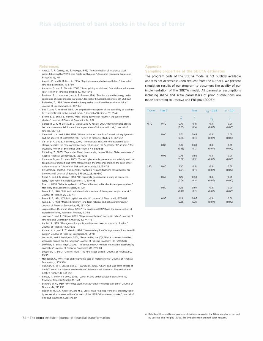
74 – The journal of financial transformation4 Details of the conditional posterior distributions used in the Gibbs sampler as derived
by Jostova and Philipov (2005) are available from authors upon request.
risk adjustment of bank stocks in the face of terror
references• Aiuppa, T., R. Carney, and T. Krueger, 1993, “An examination of insurance stock
prices following the 1989 Loma Prieta earthquake,” Journal of Insurance Issues and
Practices, 16, 1-14
• Asquith, P., and D. Mullins, Jr., 1986, “Equity issues and offering dilution,” Journal of
Financial Economics, 15, 61-89
• Avramov, D., and T., Chordia, 2006, “Asset pricing models and financial market anoma-
lies,” Review of Financial Studies, 19, 1001-1040
• Boehmer, E., J. Musumeci, and A. B. Poulsen, 1991, “Event-study methodology under
conditions of event-induced variance,” Journal of Financial Economics, 30, 253-272
• Bollerslev, T., 1986, “Generalized autoregressive conditional heteroskedasticity,”
Journal of Econometrics, 31, 307-327
• Bos, T., and P. Newbold, 1984, “An empirical investigation of the possibility of stochas-
tic systematic risk in the market model,” Journal of Business, 57, 35-41
• Brown, S. J., and J. B. Warner, 1985, “Using daily stock returns – the case of event
studies,” Journal of Financial Economics, 14, 3-31
• Campbell, J. Y., M. Lettau, B. G. Malkiel, and X. Yexiao, 2001, “Have individual stocks
become more volatile? An empirical exploration of idiosyncratic risk,” Journal of
Finance, 56, 1-43
• Campbell, J. Y., and J. Mei, 1993, “Where do betas come from? Asset pricing dynamics
and the sources of systematic risk,” Review of Financial Studies, 6, 567-592
• Carter, D. A., and B. J. Simkins, 2004, “The market’s reaction to unexpected, cata-
strophic events: the cases of airline stock returns and the September 11th attacks,” The
Quarterly Review of Economics and Finance, 44, 539-558
• Choudhry, T., 2005, “September 11 and time-varying beta of United States companies,”
Applied Financial Economics, 15, 1227-1242
• Cummins, D., and C. Lewis, 2003, “Catastrophic events, parameter uncertainty and the
breakdown of implicit long-term contracting in the insurance market: the case of ter-
rorism insurance,” Journal of Risk and Uncertainty, 26, 153-178
• De Nicolo, G., and M. L. Kwast, 2002, “Systemic risk and financial consolidation: are
they related? Journal of Banking & Finance, 26, 861-880
• Dodd, P., and J. B. Warner, 1983, “On corporate governance: a study of proxy con-
tests,” Journal of Financial Economics, 11, 401-438
• Dow, J., 2000, “What is systemic risk? Moral hazard, initial shocks, and propagation,”
Monetary and Economic Studies, 18, 1-24
• Fama, E. F., 1970, “Efficient capital markets: a review of theory and empirical work,”
Journal of Finance, 25, 383-417
• Fama, E. F., 1991, “Efficient capital markets: II,” Journal of Finance, 46, 1575-1617
• Fama, E. F., 1998, “Market Efficiency, long-term returns, and behavioral finance,”
Journal of Financial Economics, 49, 283-306
• Jagannathan, R., and Z. Wang, 1996, “The conditional CAPM and the cross-section of
expected returns, Journal of Finance, 5, 3-53
• Jostova, G., and A. Philipov, 2005, “Bayesian analysis of stochastic betas,” Journal of
Financial and Quantitative Analysis, 40, 747-787
• Kaplan, S., 1989, “Management buyouts: evidence on taxes as a source of value,”
Journal of Finance, 44, 611-632
• Korwar, A. N., and R. W. Masulis, 1986, “Seasoned equity offerings: an empirical investi-
gation,” Journal of Financial Economics, 15, 91-118
• Lettau, M., and S. Ludvigson, 2001, “Resurrecting the (C)CAPM: a cross-sectional test
when risk premia are timevarying,” Journal of Political Economy, 109, 1238-1287
• Lewellen, J., and S. Nagel, 2006, “The conditional CAPM does not explain asset-pricing
anomalies,” Journal of Financial Economics, 82, 289-314
• Loughran, T., and J. R. Ritter, 1995, “The new issues puzzle,” Journal of Finance, 50,
23-50
• Mandelker, G., 1974, “Risk and return: the case of merging firms,” Journal of Financial
Economics, 1, 303-336
• Richman, V., M. R. Santos, and J. T. Barkoulas, 2005, “Short- and long-term effects of
the 9/11 event: the international evidence,” International Journal of Theoretical and
Applied Finance, 8, 947-958
• Santos, T., and P. Veronesi, 2005, “Labor income and predictable stock returns,”
Review of Financial Studies, 19, 1-44
• Schwert, W. G., 1989, “Why does stock market volatility change over time,” Journal of
Finance, 44, 1115-1153
• Shelor, R. M., D. C. Anderson, and M. L. Cross, 1992, “Gaining from loss: property-liabili-
ty insurer stock values in the aftermath of the 1989 California earthquake,” Journal of
Risk and Insurance, 59:3, 476-87
Appendixsampling properties of the sBETA estimatesThe program code of the SBETA model is not publicly available
and was not accessible upon request from the authors. We present
simulation results of our program to document the quality of our
implementation of the SBETA model. All parameter assumptions
including shape and scale parameters of prior distributions are
made according to Jostova and Philipov (2005)4.
True α True δ True sβ = 0.25 s = 0.01
^ ^ ^ ^ α δ sβ s
0.70 0.40 0.70 0.31 0.31 0.01
(0.05) (0.14) (0.07) (0.00)
0.60 0.71 0.49 0.31 0.01
(0.06) (0.14) (0.07) (0.00)
0.80 0.72 0.69 0.31 0.01
(0.12) (0.13) (0.07) (0.00)
0.95 0.78 0.85 0.31 0.01
(0.37) (0.12) (0.07) (0.00)
1.30 0.40 1.30 0.31 0.31 0.01
(0.04) (0.14) (0.07) (0.00)
0.60 1.29 0.50 0.31 0.01
(0.06) (0.14) (0.07) (0.00)
0.80 1.28 0.69 0.31 0.01
(0.12) (0.13) (0.07) (0.00)
0.95 1.24 0.85 0.31 0.01
(0.36) (0.11) (0.07) (0.00)

75
Macroeconomic risk — sources and distributions according to a DsGE model of the E.U.David Meenagh
Cardiff University
Patrick MinfordProfessor of Applied Economics, Cardiff University,
and CEPR
Michael WickensProfessor of Economics, Cardiff University,
University of York, and CEPR
AbstractWe use a recent DSGE model of the E.U., which has reasonably satis-
fied dynamic testing, to identify the sources of risk in the economy
and to describe the resulting stochastic distributions for key macro
variables. We discuss the implications of this model for policy
responses to recent commodity and banking shocks.
Part 1

76 – The journal of financial transformation
Macroeconomic risk — sources and distributions according to a DsGE model of the E.U.
In the course of the past two years the E.U. economies have been
hit by two large shocks: a surge in commodity and oil prices, and
the ‘credit crunch’ resulting from the sub-prime banking crisis.
The first of these has as its forerunners the large commodity/oil
shocks of the 1970s and early 1980s. Precedents for the second
are to be found in the Savings and Loans crisis of the U.S. in the
latter 1980s, the Scandinavian banking crises of the early 1990s,
and the Asian crisis of 1998. Nevertheless, no one shock is ever
exactly like any other. Not only do many shocks hit economies,
besides those of the type we have recently seen, but even when
they are of the same type they differ in scale and details, as these
precedents illustrate.
This paper is a preliminary attempt to understand the sources of
shocks and their resulting stochastic distributions for key macro
and financial variables. Since these shocks work via their effects
on economies we use a model of the economy both to identify the
shocks and to pin down their transmission via the economy. Why
preliminary? Surely one might say that macroeconomic research
has had plenty of time to sort out a definitive model of the world
economy able to provide these answers? Unfortunately while previ-
ous research has indeed produced models of the world economy of
much interest, recent research has undermined faith in the basis
of these models, especially because of their loose foundations in
aggregate demand and supply, and has set out an agenda of ‘micro-
founded’ modeling which has followed many twists and turns as it
has tried both to follow the requirements of theory and also to fit
the facts. However, we believe that in the past few years serious
progress has been made in finding convincing theories that also
fit the facts. In this paper we describe a model of the E.U., which
embodies this progress and we set out its implications for the
sources and results of shocks.
This model is notionally complete as a description of the E.U. in the
sense that all shocks are accounted for. That is, all the variables of
interest are either explained by other variables or by shocks (the
unexplained elements that are omitted from the model). However, it
has obvious limitations. The most obvious is that it is a closed econ-
omy model. Trade and capital movements to and from the rest of
the world are not explicitly modeled. Instead they enter the shocks.
For example, net trade movements enter the shock to aggregate
demand in the GDP identity while net capital movements (and the
foreign returns that partly drive them) enter the monetary sector
through the shock to interest rates as notionally ‘set by monetary
policy’ according to a ‘Taylor Rule’ (supposedly describing how
the central banks move interest rates in response to inflation and
output movements). In spite of this, and of other limitations that
will emerge, this model is impressive enough both in its theoretical
foundations and its empirical performance for its implication to be
worth exploring in some detail.
The smets-Wouters DsGE model of the EU and its empirical performanceIn a notable recent contribution Smets and Wouters (2003) proposed
a dynamic stochastic general equilibrium (DSGE) model of the E.U.
which they estimated by Bayesian methods after allowing for a
complete set of pre-specified, but ad hoc, stochastic shocks. They
reported that, based of measures of fit and dynamic performance,
their model was superior in performance both to a Bayesian and a
standard VAR (vector auto regression). In this paper we look careful-
ly at their innovative model and review its performance, using a new
evaluation procedure that is suitable for either a calibrated or, as
here, an estimated structural model. The method is based on indirect
inference. It exploits the properties of the model’s error processes
through bootstrap simulations. We ask whether the simulated data
of a calibrated or an estimated structural model, treated as the null
hypothesis, can explain the actual data where both are represented
by the dynamic behavior of a well-fitting auxiliary model such as a
VAR. Our proposed test statistic is a multi-parameter Portmanteau
Wald test that focuses on the structural model’s overall capacity to
replicate the data’s dynamic performance.
The Smets-Wouters (SW) model follows the model of Christiano
et al. (2005) for the U.S. but is fitted to the data using Bayesian
estimation methods that allow for a full set of shocks. It is a
New-Keynesian model. It is based on the new Neo-Keynesian
Synthesis involving a basic real business cycle framework under
imperfect competition in which there are menu costs of price and
wage change modeled by Calvo contracts and a backward-looking
indexation mechanism; monetary policy is supplied by an interest-
rate setting rule. The effect is to impart a high degree of nominal
rigidity to the model, both of prices and inflation. A central tenet
of New-Keynesian authors is that this is necessary in order to fit
the dynamic properties of the data which are characterized by
substantial persistence in output and inflation, and hump-shaped
responses to monetary policy shocks. In this paper we probe this
argument. Specifically, we compare the SW model with a flexprice
version in which prices and wages are flexible and there is a physi-
cal one-quarter lag in the arrival of macro information. Thus our
alternative model is a type of ‘New Classical’ model. We also assess
the contribution of the ad hoc structural shocks assumed by Smets
and Wouters to the success of their structural model.
Indirect inference has been widely used in the estimation of struc-
tural models [Smith (1993), Gregory and Smith (1991), Gregory and
Smith (1993), Gourieroux et al. (1993), Gourieroux and Monfort
(1995) and Canova (2005)]. Here we make a different use of indi-
rect inference as our aim is to evaluate an already estimated or
calibrated structural model. The common element is the use of an
‘auxiliary’ model. In estimation the idea is to choose the parameters
of the structural model so that when this model is simulated it gen-
erates estimates of the auxiliary model similar to those obtained

77
from actual data. The optimal choices of parameters for the struc-
tural model are those that minimize the distance between a given
function of the two sets of estimated coefficients of the auxiliary
model. Common choices of this function are the actual coefficients,
the scores, or the impulse response functions. In model evalua-
tion the parameters of the structural model are given. The aim is
to compare the performance of the auxiliary model estimated on
simulated data from the given structural model with the perfor-
mance of the auxiliary model when estimated from actual data. The
comparison is based on the distributions of the two sets of param-
eter estimates of the auxiliary model, or of functions of these esti-
mates. Using this method we find that the SW model succeeds best
in replicating the dynamic behavior of the data when its extreme
wage/price stickiness is replaced almost entirely by a New Classical
set up. It turns out that only small imperfectly competitive sectors
(around 5%) are required in both the output and labor markets to
achieve a rather good fit to the dynamics of the data. As it were, a
little imperfection and stickiness goes a long way. The overall model
embodies essentially all the features of a New Classical model
but with much more damped inflation and interest rate behavior
because the element of stickiness both dampens price behavior
directly and indirectly via moderating the variability of price/wage
expectations. The overall dampening of wage/price fluctuations is
thus a multiple of the stickiness introduced.
The smets-Wouters DsGE model of the E.U.Following a recent series of papers, Smets and Wouters (2003)
(SW) have developed a DSGE model of the E.U. This is in most ways
an RBC model but with additional characteristics that make it New
Keynesian. First, there are Calvo wage- and price-setting contracts
under imperfect competition in labor and product markets, togeth-
er with lagged indexation. Second, there is an interest-rate setting
rule with an inflation target to set inflation. Third, there is habit
formation in consumption.
Ten exogenous shocks are added to the model. Eight (technical
progress, preferences, and cost-push shocks) are assumed to fol-
low independent AR(1) processes. The whole model is then esti-
mated using Bayesian procedures on quarterly data for the period
1970q1–1999q2 for seven Euro Area macroeconomic variables:
GDP, consumption, investment, employment, the GDP deflator, real
wages, and the nominal interest rate. It is assumed that capital and
the rental rate of capital are not observed. By using Bayesian meth-
ods it is possible to combine key calibrated parameters with sample
information. Rather than evaluate the DSGE model based only on
its sample moment statistics, impulse response functions are also
used. The moments and the impulse response functions for the
estimated DSGE model are based on the median of ten thousand
simulations of the estimated model.
We applied our testing procedure to this model using throughout the
same data for the period 1970–1999 as SW and the same detrended
series obtained by taking deviations of all variables from a mean or
a linear trend. We begin by estimating a VAR on the observed data,
using the five main observable variables: inflation (quarterly rate),
interest rate (rate per quarter), output, investment, and consump-
tion (capital stock, equity returns, and capacity utilization are all
constructed variables, using the model’s identities; we omit real
wages and employment from the VAR), all in units of percent devia-
tion from trend. We focus on a VAR(1) in order to retain power for
our tests, this yields 25 coefficients, apart from constants1.
We now turn to the actual errors derived from using the observed
data. We use ‘actual errors’ from now on to describe the model’s
1 We tried higher order VARs, up to third order, but they are not used for model test-
ing. For example, a VAR(3) generally shows all models as passing handsomely, having
no less than 75 coefficients. The power of the test is extremely weak.
2 Under our procedure the exact way to derive these is to generate the model’s own
expected variables conditional on the available information in each period. These
errors being calculated, AR processes are estimated for them. The SW model can
then be bootstrapped using the random elements in these error processes. To find
these errors one needs to iterate between the errors used to project the model
expectations and the resulting errors when these expectations are used to calculate
the errors. This procedure is complex and has so far produced large and implausible
errors. In practice we used an alternative procedure to calculate the errors, which
avoids this need to iterate. We projected the expected variables from the VAR(1)
estimated above. Since this VAR is not the exact model but is merely a convenient
description of the data, under the null hypothesis of the structural DSGE model these
expected variables will be the model’s true expectations plus approximation errors.
We conjecture that this will lower the power of the Wald statistic but only negligibly;
to test this conjecture heuristically we raise the order of the VAR used to project the
expectations and see whether it affects the results. We know that the model has a
VAR representation if it satisfies the Blanchard-Kahn conditions for a well-behaved
rational expectations model, as is assumed and checked by Dynare. As the order of
the VAR rises it converges on this exact representation, steadily reducing the degree
of the approximation. Hence if the results do not change as the VAR order rises, it
implies that the approximation error has trivial effects. This is what we found when
we raised the order from 1 to 3 (for example, the Wald statistic moved from 92.9
to 94.6; the model’s interest rate variance lower 95% bound moved from 0.024 to
0.025). We are also investigating further ways to solve for the exact expectations.
It should also be noted that we excluded the first 20 error observations from the
sample because of extreme values. We also smoothed two extreme error values in
Q. Thus our sample for both bootstraps and data estimation was 98 quarters, i.e.
1975(1)-1999(2).
Macroeconomic risk — sources and distributions according to a DsGE model of the E.U.
0 20 40 60 80 100-5
0
5
10Consumption
0 20 40 60 80 100-20
-10
0
10
20Investment
0 20 40 60 80 100-1
0
1
2Inflation
0 20 40 60 80 100-10
-5
0
5
10Wages
0 20 40 60 80 100-2
-1
0
1
2Government spending
0 20 40 60 80 100-5
0
5Productivity
0 20 40 60 80 100-2
0
2
4Interest rate
Resids
Data
Figure 1 – Single equation errors from SW model

78 – The journal of financial transformation
Macroeconomic risk — sources and distributions according to a DsGE model of the E.U.
structural residuals, that is the residual in each equation given the
actual data and the expected variables in it2 (Figure 1). There are six
behavioral errors: consumption, investment, productivity, interest
rates (monetary policy), wage- and price-setting, and one exogenous
process, ‘government spending,’ which is the residual in the goods
market-clearing equation (or ‘GDP identity’) and therefore includes
net trade as discussed earlier. The first error is that of the Euler
equation and has a standard error of 0.5(%), roughly half as much
again as assumed by SW [see Canzoneri et al. (2007) on the peculiari-
ties of actual Euler equation errors], that for investment in the sec-
ond has a standard error of 1.2%, around ten times that assumed by
SW. Furthermore the AR coefficients (ρs) of the structural residuals
are very different. There is hardly any persistence in the estimated
residuals for consumption and investment, unlike the high persis-
tence assumed by SW. In contrast, the actual inflation and Taylor
Rule errors are persistent and not zero, as assumed. Figure 2 shows
the comparison between SW’s assumed shocks and those shown in
Figure 1. These differences turned out to be an important factor in
the tests we carried out as we found that the model’s originally good
performance in our tests came from the errors used by SW based
largely on their priors. Once the true errors were substituted the
original model was rejected and we only achieved acceptance once
we had altered the model towards a predominantly New Classical
form with only a small degree of stickiness.
Using these actual errors we proceeded to bootstrap this ‘mixed
NC’ model. We found that the properties of the errors are the key
element in the success or failure of both SWNK and SWNC in these
tests. The more the error properties conform to NK priors, with
dominant demand shocks, the better the SWNK model performs
and the worse the SWNC does. In contrast, the more the errors
conform to New Classical priors, the better the SWNC performs and
the worse SWNK does. When the error properties are derived from
observed data, both models have difficulty fitting the data, though
SWNC model is probably the closest to doing so. What is the expla-
nation for these results?
In the SWNK model, because capacity utilization is flexible,
demand shocks (consumption/investment/money) dominate out-
put and — via the Phillips Curve — inflation, then — via the Taylor
Rule — interest rates. Supply shocks (productivity, labor supply,
wages/inflation mark-ups) play a minor role as ‘cost-push’ infla-
tion shocks as they do not directly affect output. Persistent
demand shocks raise ‘Q’ persistently and produce an ‘investment
boom’ which, via demand effects, reinforces itself. Thus the model
acts as a ‘multiplier/accelerator’ of demand shocks. Demand
shocks therefore dominate the model, both for real and nominal
variables. Moreover, in order to obtain good model performance
for real and nominal data, these demand shocks need to be of suf-
ficient size and persistence.
In the SWNC model an inelastic labor supply causes output variation
to be dominated by supply shocks (productivity and labor supply) and
investment/consumption to react to output in a standard RBC man-
ner. These reactions, together with demand shocks, create market-
clearing movements in real interest rates and — via the Taylor Rule
— in inflation. Supply shocks are prime movers of all variables in the
SWNC model, while demand shocks add to the variability of nominal
variables. In order to mimic real variability and persistence, suitably
sized and persistent supply shocks are needed to mimic the limited
variability in inflation and interest rates, only a limited variance in
demand shocks is required, and to mimic their persistence the supply
shocks must be sufficiently autocorrelated.
The observed demand shocks have too little persistence to cap-
ture the variability of real variables in the SWNK model, but they
generate too much variability in nominal variables in the SWNC
model. The observed supply shocks matter little for the SWNK but
are about right in size and persistence for the real variables in the
SWNC. The implication is that the flexibility of prices and wages
may lie somewhere between New Keynesian and the New Classical
models. For example, adding a degree of price and wage stickiness
to the SWNC model would bring down the variance of nominal vari-
ables, and boost that of real variables in the model.
A natural way to look at this is to assume that wage and price
setters find themselves supplying labor and intermediate output
partly in a competitive market with price/wage flexibility, and
partly in a market with imperfect competition. We can assume that
the size of each sector depends on the facts of competition and
do not vary in our sample. The degree of imperfect competition
could differ between labor and product markets. For the exercise
here we will initially assume that it is the same in each market
and given by a single free parameter, v. This implies that the price
and wage equations will be a weighted average of the SWNK and
SWNC equations, with the weights respectively of (1-v) and v. We
will also assume that the monetary authority uses this parameter
to weight its New Keynesian and New Classical Taylor Rules as
we have found that different values of the parameter v work best
for a competitive (NC) model and an imperfect competition (NK)
economy. In practice we can think of the weight v as giving the
extent of the NC (competitive) share of the economy3.
Variances cons Inv Inflation Wage Gov Prod Taylor rule
Data variances 0.26 1.52 0.0007 0.278 0.141 0.091 0.227
SW variances 0.088 0.017 0.026 0.081 0.108 0.375 0.017
Ratio 2.9 89 0.03 3.4 1.3 0.24 13.4
ρ
Data -0.101 0.063 0.154 -0.038 0.751 0.940 0.565
SW 0.886 0.917 0 0 0.956 0.828 0
Figure 2 – Variances of innovations and AR coefficients (rhos) of shocks
(data-generated versus SW assumed shocks)

79
Macroeconomic risk — sources and distributions according to a DsGE model of the E.U.
We now choose a value of v for which the combined model is clos-
est to matching the data variances while also passing the Wald
test. This is an informal use of indirect inference that provides
a broader criterion which better reflects our concerns with the
models’ performance than simply applying a Wald score to, for
example, the VAR coefficients. The optimal value turns out to be
0.94. This implies quite a small NK sector of only 6% of the econ-
omy, but it is sufficient to bring the overall economy’s properties
close to the dynamic facts. We allowed the weight to be further
varied around this to generate an optimum performance: in labor
markets (vW = 0.08), product markets (vP = 0.06), and monetary
policy (vm = 0.04). We now consider how good a fit this is.
The key difference is the ability of the model to replicate the vari-
ances in the data: all the data variances lie within the model’s 95%
bounds (Figure 3). The model, therefore, satisfies the necessary
basic conditions for us to take it seriously; it produces behavior of
the right size for both real and nominal variables and the structural
errors are generated from the model using the observed data.
The model is still rejected, as are all versions of the Smets-Wouters
model, by the Wald test (a test of where the joint set of VAR coef-
ficients lies in the full joint distribution of the VAR coefficients
according to the structural model) which is 100. A weaker test sets
the covariances of this distribution to zero; under this the test
becomes a geometric average of the t-statstistics on each VAR
coefficient (a ‘joint t-test’ as we might call it). Under this joint t-test
the statistic is 90.8 with just three VAR coefficients lying outside
their 95% bounds. The main discrepancy is the partial autocorrela-
tion of interest rates which the model underpredicts. The other two
coefficients involve the cross-effects of output and interest rates
on inflation, but they are only moderately outside their bounds.
The variance decomposition of real variables is now heavily skewed
towards being caused by supply shocks with 73% of the output
variance being due in the model to labor supply and productivity
shocks. In contrast, nominal variables are dominated by demand
shocks with 74% of the variance of inflation due in the model to
the shocks to the Taylor Rule. Being the sum of a real variable and
expected inflation, about a third of the variance of nominal inter-
est rates is due to productivity and labor supply shocks, with the
remainder due to shocks to the Taylor Rule (also a third) and to
other demand shocks. Thus supply shocks largely dominate real
variables while demand shocks largely dominate nominal variables.
The model bounds for the VAR impulse response functions enclose
many of the data-based IRFs for the three key shocks: labor supply,
productivity, and shocks to the Taylor Rule. The main discrepancies
in response to supply shocks are the longer-term predictions of
interest rates and inflation which in the data wander further from
3 Formally, we model this as follows. Each household spends a proportion vW of its time
working in the ‘unionized’ sector of the labor market; this proportion has wages set
by its union according to the Calvo wage-setting equation. The rest of its time is spent
working in the competitive labor market where wages are equal to their marginal dis-
utility of work. Its wage demands are then passed to a ‘labor manager’ who bundles its
labor into a fixed coefficients labor unit (each labor type is complementary — i.e., skilled
craft and general work) and charges for it the weighted average wage demand. Firms
then buy these labor units off the manager for use in the firm. Similarly, each firm sells
a proportion vP of its output in an imperfectly competitive market and the rest in a
competitive market. It prices one according to its mark-up equation on marginal costs,
in the other equal to marginal costs. Its product is then sold to a retail bundler who
combines it in fixed proportions and sells it on at the weighted average price. Notice
that apart from these equations the first-order conditions of households and firms will
be unaffected by what markets they are operating in.
consumption Investment Inflation output Interest rate
Actual 5.4711 37.1362 0.2459 3.6085 0.3636
Lower 1.7200 20.7905 0.2292 1.5284 0.2036
Upper 13.7364 172.3241 0.8405 11.3359 0.7146
Mean 5.0452 69.2529 0.4425 4.4535 0.3764
Prod cons Gov Inv Price labor Wage Taylor Total mark-up supply mark-up rule
C 26.041 6.513 0.413 2.903 0.068 49.568 0.000 14.494 100
I 13.792 0.054 0.158 34.390 0.003 33.683 0.000 17.920 100
K 20.767 0.033 0.121 18.648 0.002 39.724 0.000 20.706 100
L 22.861 4.391 6.197 2.762 0.033 54.190 0.000 9.566 100
π 1.087 11.414 0.556 0.469 6.091 6.246 0.002 74.135 100
Q 9.344 5.299 1.284 12.582 1.428 43.131 0.001 26.931 100
R 5.141 20.320 2.297 2.421 6.155 27.080 0.011 36.574 100
rk 8.240 32.100 1.832 9.411 0.960 17.745 0.004 29.708 100
W 14.806 36.872 0.182 2.092 1.301 9.770 0.008 34.969 100
Y 24.531 4.518 3.780 3.538 0.052 48.228 0.000 15.352 100
Actual estimate lower bound Upper bound state t-stat*
ACC 0.88432 0.26572 1.02827 True 1.17662
ACI -0.09612 -0.92015 1.19403 True -0.39647
ACπ 0.01867 -0.30244 0.08489 True 1.27573
ACY 0.07935 -0.36553 0.28805 True 0.72452
ACR -0.00824 -0.33625 -0.00284 True 1.83460
AIC -0.02461 -0.06640 0.06491 True -0.75793
AII 0.91856 0.68054 1.05976 True 0.30909
AIπ -0.01074 -0.02810 0.05323 True -1.14494
AIY -0.01190 -0.04254 0.07168 True -0.91032
AIR -0.00504 -0.01937 0.04928 True -1.13906
AπC -0.04105 -0.28473 1.84441 True -1.51365
AπI -0.71538 -1.68976 4.13846 True -1.38882
Aππ 0.68194 0.44617 1.57336 True -1.23414
AπY -0.00692 0.08981 1.93824 False -2.00415
AπR -0.01605 0.10374 1.04049 False -2.51828
AYC 0.21989 -0.27066 0.71764 True 0.03638
AYI 0.38855 -1.34895 1.33299 True 0.50045
AYπ 0.05457 -0.25489 0.27741 True 0.25731
AYY 0.93795 0.38837 1.25734 True 0.42118
AYR 0.06281 -0.19508 0.25990 True 0.19567
ARC -0.37666 -2.04721 0.26606 True 0.87186
ARI -0.97612 -4.17678 2.09513 True 0.07900
ARπ -0.05704 -1.05222 0.07775 True 1.45411
ARY -0.40669 -2.12602 -0.15480 True 1.28935
ARR 0.89695 -0.52286 0.45459 False 3.79338
Joint t-test 90.8
*t-stat from bootstrap mean
Figure 3 – Variance of data and bootstraps for the weighted model
Figure 5 – Variance decomposition for weighted model
Figure 4 – VAR parameters and model bootstrap bounds (weighted model)

80 – The journal of financial transformation
Macroeconomic risk — sources and distributions according to a DsGE model of the E.U.
equilibrium than in the model. Again, apart from the longer-term
interest rate predictions, all data-based IRFs for the Taylor Rule
demand shock lie inside; these are (as we saw from the VAR coef-
ficient) a lot more persistent in the data than in the model. Hence
the model performance based on the IRFs is fairly good, with the
main weakness in the interest rate prediction.
Looking at cross-correlations for the real variables, we find that the
data-based correlations all lie inside the model’s bounds as they did
for the NC model. Now, however, the weights for NK formulation of
price stickiness, although small, produce behavior in the nominal
variables that is almost within the 95% bounds of the weighted
model (only the interest rate cross-correlation with output lies much
outside).
To summarize, we find that a small weight on the NK formulation
of price stickiness suffices to get the mixed New Classical-New
Keynesian model to pass our tests. There are still some failures, so
that the problem of finding a fully satisfactory specification in prin-
ciple remains. Nonetheless, within the specifications at our disposal
here, we can say that the E.U. economy appears to be closest to a
New Classical specification and that this model gets the closest any
modern micro-founded DSGE model has ever got to the data.
Using the sW MIXED nc model to analyze the economy’s risksWhat has the model got to say about the two big shocks of
2007–8?
A useful way of introducing the model’s behavior is to see what it
has to say about the big current shocks mentioned at the start of
this paper. Our estimates of the shocks are intended to be illustra-
tive of the order of magnitude rather than in any way precise. We
assume that commodity price inflation would have added about 3%
to headline inflation after a year — we model this as an equivalent
shock to productivity since commodity prices do not enter the
model as such.
For the credit crunch shock we assume 20% of borrowers were
marginal and unable to obtain normal credit facilities after the
crisis hit; we assume they could obtain credit on credit card terms
(say around 30% p.a.) only. Other borrowers faced a rise in interest
rates due to the inter-bank risk premium which has varied between
50 and 200 basis points during this crisis so far, as compared with
a negligible value beforehand. There was also some switching of
borrowers away from fixed-rate mortgages to higher variable rate
ones. Overall, we assume these other borrowers faced a rise of
2% in rate costs. Averaging across the two categories, we get an
0 5 10 15 20-0.5
0
0.5Consumption
0 5 10 15 20-0.5
0
0.5
1Investment
0 5 10 15 20-0.2
0
0.2Inflation
0 5 10 15 20-0.5
0
0.5Output
0 5 10 15 20-0.1
0
0.1Interest Rate
Figure 6 – Taylor rule shock to weighted model
5 10
0
0.2
0.4
0.6
0.8
C v. C(-i)
5 10
0
0.2
0.4
0.6
0.8
I v. I(-i)
5 10-0.2
0
0.2
0.4
0.6
0.8P v. P(-i)
5 10
0
0.2
0.4
0.6
0.8
Y v. Y(-i)
5 10-0.2
0
0.2
0.4
0.6
0.8
R v. R(-i)
2 4 6 810
0
0.2
0.4
0.6
0.8
C v. Y(-i+1)
2 4 6 810
0
0.2
0.4
0.6
0.8
I v. Y(-i+1)
2 4 6 810
-0.5
0
0.5
P v. Y(-i+1)
2 4 6 810
-0.5
0
0.5
R v. Y(-i+1)
2 4 6 8100.6
0.7
0.8
0.9
C v. Y(+i-1)
2 4 6 810
0.5
0.6
0.7
0.8
0.9
I v. Y(+i-1)
2 4 6 810
-0.4
-0.2
0
0.2
0.4
P v. Y(+i-1)
2 4 6 810
-0.4
-0.2
0
0.2
0.4
R v. Y(+i-1)
0 5 10 15 20-0.5
0
0.5
1Consumption Investment
0 5 10 15 20-1
0
1
2
0 5 10 15 20-0.1
0
0.1Inflation
0 5 10 15 20-0.5
0
0.5Output
0 5 10 15 20-0.2
0
0.2Interest Rate
Figure 8 – Cross-correlations for flex-price model (with dummied data)
Figure 7 – Productivity shock to weighted model
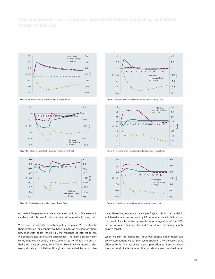
81
Macroeconomic risk — sources and distributions according to a DsGE model of the E.U.
estimated 6% per annum rise in average credit costs. We assume it
carries on at this level for six quarters before gradually dying out.
What are the possible monetary policy responses? To estimate
their effects on the economy we have to make an assumption about
how monetary policy reacts (i.e., the response of interest rates).
We compare two alternative approaches. The main approach cur-
rently followed by central banks committed to inflation targets is
that they react according to a ‘Taylor Rule’ in which interest rates
respond mainly to inflation, though also somewhat to output. We
have, therefore, embedded a simple Taylor rule in the model in
which real interest rates react by 1.5 times any rise in inflation from
its target. An alternative approach, more suggestive of the ECB,
is that interest rates are changed to meet a fixed money supply
growth target.
When we run the model for these two shocks under these two
policy assumptions we get the results shown in the six charts above
(Figures 9-14). The last chart in each part (Figures 11 and 14) show
the sum total of effects when the two shocks are combined. In all
-1.5
-1.0
-0.5
0.0
0.5
1.0
1.5
1 2 3 4 5 6 7 8 9 10 11 12 13 14 15 16 17 18 19 20
%
-6.0
-4.0
-2.0
0.0
2.0
4.0
6.0
% p
.a.
InflationInterest RateOutput
-5.0
-4.0
-3.0
-2.0
-1.0
0.0
1.0
1 2 3 4 5 6 7 8 9 10 11 12 13 14 15 16 17 18 19 20
%
-20.0
-16.0
-12.0
-8.0
-4.0
0.0
4.0
% p
.a.
InflationInterest RateOutput
-7.0
-6.0
-5.0
-4.0
-3.0
-2.0
-1.0
0.0
1.0
1 3 5 7 9 11 13 15 17 19
%
-28.0
-24.0
-20.0
-16.0
-12.0
-8.0
-4.0
0.0
4.0
% p
.a.
InflationInterest RateOutput
-2.0
-1.5
-1.0
-0.5
0.0
0.5
1.0
1 3 5 7 9 11 13 15 17 19
%
-8.0
-6.0
-4.0
-2.0
0.0
2.0
4.0
% p
.a.
InflationInterest RateOutput
-2.5
-2.0
-1.5
-1.0
-0.5
0.0
0.5
1.0
1.5
1 2 3 4 5 6 7 8 9 10 11 12 13 14 15 16 17 18 19 20
%
-10.0
-8.0
-6.0
-4.0
-2.0
0.0
2.0
4.0
6.0
% p
.a.
InflationInterest RateOutput
-4.0
-3.0
-2.0
-1.0
0.0
1.0
2.0
1 3 5 7 9 11 13 15 17 19
%
-16.0
-12.0
-8.0
-4.0
0.0
4.0
8.0
% p
.a.
InflationInterest RateOutput
Figure 9 – Productivity fall (weighted model, Taylor Rule)
Figure 10 – Credit crunch shock (weighted model, Taylor Rule)
Figure 11 – Total episode (weighted model, Taylor Rule)
Figure 12 – Productivity fall (weighted model, money supply rule)
Figure 13 – Credit crunch shock (weighted model, money supply rule)
Figure 14 – Total episode (weighted model, money supply rule)

82 – The journal of financial transformation
our charts we show effects quarter by quarter (the horizontal axis
measures time in quarters). On the vertical axis the left hand scale
applies to output and shows the percent effect on output, the right
hand scale applies to interest rates and inflation and shows the
effect in percent per annum. Interest rates shown are those that
consumers pay (i.e., under the credit crunch they include the esti-
mated direct effect of the credit crunch).
Taylor rule resultsUnder the pure Taylor Rule policy we find that interest rates rise sub-
stantially in response to the commodity price shock. This is because
although there is a recessionary effect it is weak compared with
the short-run effect on inflation. However, in response to the credit
crunch shock, interest rates inclusive of the credit crunch effect fall
markedly; this is in reaction to the deflationary effect of the shock,
creating both a sharp recession and a sharp fall in inflation. Since
the direct effect of the credit crunch on interest rates is initially 6%,
to get market rates to fall would require an even bigger fall in base
rates — in effect to below zero. While that is technically possible, it is
in practice unlikely. Nevertheless it is interesting to see how sharply
monetary policy would need to move under the Taylor Rule, and then
of course we did not see the credit crunch shock in isolation. When
one adds the two shocks together, the interest rate inclusive of the
credit effect remains about constant, which means that base rates
are cut to match the credit crunch effect while it is occurring. Plainly
this means large cuts in base rates (effectively to around zero) in the
attempt to offset the rise in interest rates charged for risk reasons.
If we look at the interest rates actually set by the ECB and the Bank
of England, it is clear that they have deviated substantially from this
Taylor Rule prescription. They barely cut base rates after August
2007 until the Lehman crisis in September 2008. This is to be com-
pared with the U.S. Fed which has tried roughly to offset the tighten-
ing credit conditions with repeated cuts in its Fed Funds target (now
set at 1%); it looks as if the Fed has roughly followed a Taylor Rule.
Money supply rule resultsWhen we apply the alternative policy of money supply targeting,
we find rather different results. Firstly, interest rates do not react
to the commodity price shock because the demand for money is
largely unaffected — the inflation rise more or less offsets the drop
in output. But secondly, interest rates inclusive of the credit crunch
rise in response to the credit crunch; interest rates only partially
offset the tightening from the rising risk premium. This is because,
as demand for money growth falls, in order to restore it to the level
of the money supply growth target, only a small cut in interest rates
is required. This reflects the strong response of money demand to
the interest rate that is usually observed (we assume here 0.075).
Adding the two together we find that interest rates do rise over the
whole episode but by a lot less than observed in practice in the E.U.,
and rather more than they observed in the U.S.
Implications for monetary policyOn the basis of our estimates and these two widely suggested rules
for monetary policy, the verdict on U.S. policy is that it has been
about right on one approach (the Taylor Rule), and a bit too loose
on the other (the money supply target). In contrast, E.U. policy has
been too tight on both rules: very much too tight on the Taylor Rule
and rather too tight on the money supply target.
The Taylor Rule is what most central banks say they are following. It
is also widely thought to be a good policy for containing inflation with-
out unduly harsh effects on output. If we take this as our main guide it
suggests that the U.S. Fed has got its approach to recent events about
right while the ECB and the Bank of England, together with most other
E.U. central banks, have set their policies rather too tight. The ECB
could reply that it pays more attention to money supply. Even if that
is the case, on this evidence it has still been rather too tight. The same
applies to the Bank and most other European central banks.
Where might this excessive tightness come from? It appears from
statements by board members of these bodies that on the European
Macroeconomic risk — sources and distributions according to a DsGE model of the E.U.
lower Upper s.D. skewness Kurtosis
output
1 Year -2.797 2.473 1.334 -0.299 3.493
3 Years -4.455 3.806 2.079 -0.356 3.727
5 Years -4.898 4.597 2.450 -0.147 2.861
25 Years -5.741 5.516 2.852 -0.110 3.028
consumption
1 Year -3.174 2.642 1.472 -0.399 3.645
3 Years -4.763 3.699 2.209 -0.421 3.562
5 Years -5.306 4.830 2.604 -0.185 2.861
25 Years -6.280 6.030 3.125 -0.093 3.216
Investment
1 Year -8.875 8.512 4.428 -0.078 3.139
3 Years -16.777 14.908 8.048 -0.251 3.455
5 Years -18.597 17.105 9.180 -0.169 2.897
25 Years -20.003 18.952 9.835 -0.108 3.447
Inflation
1 Year -1.051 1.143 0.560 0.150 2.949
3 Years -1.334 1.411 0.699 0.114 2.913
5 Years -1.438 1.455 0.740 0.044 3.035
25 Years -1.393 1.452 0.731 0.056 2.836
Interest rate
1 Year -0.933 1.005 0.496 0.148 2.975
3 Years -1.189 1.285 0.629 0.143 3.045
5 Years -1.231 1.330 0.655 0.152 3.082
25 Years -1.301 1.312 0.672 -0.004 2.732
Value of capital
1 Year -2.059 2.264 1.094 0.216 3.228
3 Years -2.396 2.553 1.266 0.122 3.063
5 Years -2.490 2.608 1.315 0.079 2.818
25 Years -2.518 2.721 1.330 0.194 3.411
Note units: % for real, % per quarter for inflation and interest rate
Figure 15 – Key measures for each distribution

83
side of the Atlantic there has been concern about losing credibility
in the face of rising ‘headline’ inflation whereas on the U.S. side of
the Atlantic credibility was felt to be safe because ‘core inflation’
was not affected by the commodity price shock. Clearly assessing
credibility requires another sort of model entirely — one that allows
for political backlash against the regime of inflation targeting
among other elements. But certainly in the context of such a severe
credit shock, the U.S. judgment seems to be valid judging by events.
Credibility has not been threatened because credit conditions have
in effect been greatly tightened by the credit shock just as the com-
modity shock was hitting. In the U.S. even the efforts of the Fed to
offset the rise in credit costs failed to do so completely.
Our assessment, based on the views of central bankers and their
advisers, has assumed that these two monetary rules represent
the best practices available. It would, therefore, be interesting to
experiment with other monetary policy rules, both evaluating their
properties in general and in the context of these shocks. That is
something that we have left for future work.
What has the model got to say about the distributions of key variables? In Figures 16 to 20, we show the raw bootstrap (demeaned) dis-
tributions of the main macro-variables up to 25 years ahead. The
pattern shows little skewness or kurtosis and is close to normality.
Near term uncertainty is limited but the full extent of it builds up
quickly, reaching its steady state within about a year. Figure 15
Macroeconomic risk — sources and distributions according to a DsGE model of the E.U.
shows the key measures for each distribution at 1 year, 3, 5, and 25
years: 95% bounds, variance, skewness, and kurtosis. (Note units:
% for real, % per quarter for inflation and interest rate). Real vari-
ables are highly correlated, as illustrated by the joint distribution of
output and consumption 12 quarters, or 3 years, ahead in Figure 23.
This is not because consumers do not attempt consumption
smoothing, as we assume habit persistence in order to increase risk
premia. Rather it is because of the exigencies of market-clearing
which drives real interest rates (and real wages) to equate a supply
that is constrained by limited stocks of labor to aggregate demand.
The fluctuations in real interest rates force consumers to closely
match consumption to available output.
In order to find a measure of risk we weight the return on equity (Q)
by the consumption-based stochastic discount factor, the marginal
utility of consumption to give Qt+12/(Ct+12 – hCt+11)s. The assumption
of habit persistence (h>0) is chosen to enhance the volatility of the
discount factor; taking a horizon of three years ahead (t+12) and find
the distribution of Qt+12/(Ct+12 – hCt+11)s. We normalize this ratio to
unity at the means of the variables Q and C; the mean of the ratio
will be less than unity. We note that consumption is highly correlated
with output at the 3-year horizon, as are all the other macroeconom-
ic aggregates — see Figure 23 which shows the joint distribution of
output with consumption. Consequently, it is clear that the stochas-
tic discount factor (which is inversely related with consumption) will
also be strongly inversely related to other outcomes. Furthermore,
negative outcomes will have low discount factors and positive out-
Figure 16 – Distribution of output
Figure 19 – Distribution of inflation
Figure 17 – Distribution of consumption
Figure 20 – Distribution of interest rate
Figure 18 – Distribution of investment
Figure 21 – Distribution of Qt+12/(Ct+12 – hCt+11)s
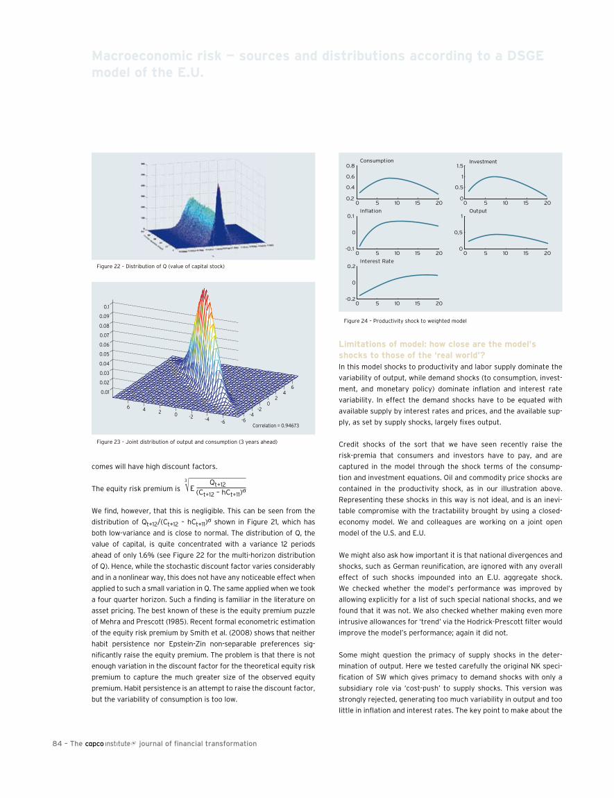
84 – The journal of financial transformation
Macroeconomic risk — sources and distributions according to a DsGE model of the E.U.
-6-4
-20
24
6
-6-4-20246
0.01
0.02
0.03
0.04
0.05
0.06
0.07
0.08
0.09
0.1
Correlation = 0.94673
Figure 22 – Distribution of Q (value of capital stock)
Figure 23 – Joint distribution of output and consumption (3 years ahead)
comes will have high discount factors.
The equity risk premium is
Qt+12E (Ct+12 – hCt+11)
s√3
We find, however, that this is negligible. This can be seen from the
distribution of Qt+12/(Ct+12 – hCt+11)s shown in Figure 21, which has
both low-variance and is close to normal. The distribution of Q, the
value of capital, is quite concentrated with a variance 12 periods
ahead of only 1.6% (see Figure 22 for the multi-horizon distribution
of Q). Hence, while the stochastic discount factor varies considerably
and in a nonlinear way, this does not have any noticeable effect when
applied to such a small variation in Q. The same applied when we took
a four quarter horizon. Such a finding is familiar in the literature on
asset pricing. The best known of these is the equity premium puzzle
of Mehra and Prescott (1985). Recent formal econometric estimation
of the equity risk premium by Smith et al. (2008) shows that neither
habit persistence nor Epstein-Zin non-separable preferences sig-
nificantly raise the equity premium. The problem is that there is not
enough variation in the discount factor for the theoretical equity risk
premium to capture the much greater size of the observed equity
premium. Habit persistence is an attempt to raise the discount factor,
but the variability of consumption is too low.
limitations of model: how close are the model’s shocks to those of the ‘real world’? In this model shocks to productivity and labor supply dominate the
variability of output, while demand shocks (to consumption, invest-
ment, and monetary policy) dominate inflation and interest rate
variability. In effect the demand shocks have to be equated with
available supply by interest rates and prices, and the available sup-
ply, as set by supply shocks, largely fixes output.
Credit shocks of the sort that we have seen recently raise the
risk-premia that consumers and investors have to pay, and are
captured in the model through the shock terms of the consump-
tion and investment equations. Oil and commodity price shocks are
contained in the productivity shock, as in our illustration above.
Representing these shocks in this way is not ideal, and is an inevi-
table compromise with the tractability brought by using a closed-
economy model. We and colleagues are working on a joint open
model of the U.S. and E.U.
We might also ask how important it is that national divergences and
shocks, such as German reunification, are ignored with any overall
effect of such shocks impounded into an E.U. aggregate shock.
We checked whether the model’s performance was improved by
allowing explicitly for a list of such special national shocks, and we
found that it was not. We also checked whether making even more
intrusive allowances for ‘trend’ via the Hodrick-Prescott filter would
improve the model’s performance; again it did not.
Some might question the primacy of supply shocks in the deter-
mination of output. Here we tested carefully the original NK speci-
fication of SW which gives primacy to demand shocks with only a
subsidiary role via ‘cost-push’ to supply shocks. This version was
strongly rejected, generating too much variability in output and too
little in inflation and interest rates. The key point to make about the
0 5 10 15 200.2
0.4
0.6
0.8Consumption Investment
0 5 10 15 200
0.5
1
1.5
0 5 10 15 20-0.1
0
0.1Inflation
0 5 10 15 200
0,5
1Output
0 5 10 15 20-0.2
0
0.2Interest Rate
Figure 24 – Productivity shock to weighted model

85
Macroeconomic risk — sources and distributions according to a DsGE model of the E.U.
role of supply shocks in the mixed NC version is that they also act as
shocks to demand via their effect on both consumption and invest-
ment plans. One can think of a sustained rise in productivity as
setting off a wave of ‘optimism’ on the demand side just as it raises
output from the supply side. Indeed the extra demand it generates
will typically exceed the extra supply and drive up real interest rates
(see the model’s deterministic IRF for a productivity shock).
In short, the model has undoubted limitations but the fact that it is
in principle complete in its treatment of shocks, theoretically well-
founded, and also fits the dynamic facts count strongly in its favor
as a tool for examining our problems.
Are there policy lessons to be learned from the model? We have examined above how monetary policy should have reacted
to the recent dual shocks hitting the world economy. We did so under
two well-known monetary policy rules, a simple Taylor Rule strictly
targeting inflation and a money supply growth rule. Empirically the
simple Taylor Rule allows the model to fit the facts best. However,
we might ask whether some other rule could have produced better
overall economic behavior from the viewpoint of households. One
such rule could be price level targeting, others could be alternative
variants of the Taylor Rule. This is something to be looked at in
later work. On the basis of its empirical performance it appears the
assumed simple reaction of real interest rates to inflation is a fairly
strong stabilizer of the economy — essentially it makes inflation and
real interest rates vary directly with each other so sharing the load
of reducing excess demand.
Another question we might ask is whether some policy environment
could have avoided the two shocks. Essentially this lies beyond this
model. Some would like to model the credit process itself. Plainly
this is not done here but it is certainly a worthwhile endeavor.
Others would like to include the regulatory framework in some way,
presumably this would accompany the modeling of the credit pro-
cess. Furthermore, commodity and oil price movements are deter-
mined in the wider world economy. Modeling these would require a
world model with a monetary and other transmission mechanisms
to an emerging market bloc. Such questions, which endogenize the
dual shocks analyzed, are for later, more ambitious work.
The model is also largely silent on fiscal policy. Government spend-
ing is exogenous, with no consumption value to households (spend-
ing has to be done for overriding reasons such as infrastructure)
and taxes are treated as ‘lump sum’ so that they have no effect on
supply. Households face fully contingent markets and so smooth
their purchases optimally across time. There is, therefore, no role
in this model for ‘Keynesian’ fiscal policy — bond-financed tax
movements have no effect and the government spending impulse
responses are weak.
conclusionIn the wake of the banking crisis, one widely-met reaction has been
that we should rip up DSGE models with no banking systems and
start again. While it is undoubtedly worthwhile to model the roles
of credit and money in the economy, one can also model the effects
of shocks to banking and money indirectly as shocks to the costs of
credit, and to the provision of money by the central bank indirectly
by the interest rate behavior it induces. This is what is done here
based on the DSGE model developed by Smets and Wouters, which
builds on the work of Woodford, Christiano, and others. We in our
turn have modified the price/wage rigidity assumptions of these
‘New Keynesian’ models, turning them back into close cousins of
‘New Classical’ models with a high degree of price/wage flexibility.
Such a model, which has a large weight on price/wage flexibility
and a small weight on rigidity, appears to best mirror the facts of
the E.U. business cycle. This ‘weighted’ model produces some fairly
plausible measures of the effects of the recent twin banking and
commodity shocks on the E.U. economy, and of the riskiness of the
macro-environment from the pure business cycle viewpoint. Like
other work on general equilibrium models of asset prices, it does
not, however, give a plausible account of asset price uncertainty.
Nonetheless, the model has interesting policy implications for the
business cycle. It emphasizes the role of monetary policy on market
interest rates and downgrades the role of fiscal activism, leaving
fiscal policy as needing to be consistent with inflation targets and
the money creation implied by interest rate behavior. Until we have
been able to develop DSGE models with explicit banking systems
that can match the data, the type of model employed here seems
to provide us with a reasonable stopgap for thinking about current
policy over the business cycle.
references• Canova, F. (2005), Methods for Applied Macroeconomic Research, Princeton University
Press, Princeton
• Canzoneri, M. B., R. E. Cumby, and B. T. Diba, 2007, “Euler equations and money
market interest rates: a challenge for monetary policy models,” Journal of Monetary
Economics, 54, 1863–1881
• Christiano, L., M. Eichenbaum, and C. Evans, 2005, “Nominal rigidities and the dynamic
effects of a shock to monetary policy,” Journal of Political Economy, 113, 1–45
• Gourieroux, C. and A. Monfort, 1995, Simulation based econometric methods, CORE
Lectures Series, Louvain-la-Neuve
• Gourieroux, C., A. Monfort, and E. Renault, 1993, “Indirect inference,” Journal of
Applied Econometrics, 8, 85–118
• Gregory, A., and G/ Smith, 1991, “Calibration as testing: inference in simulated macro
models,” Journal of Business and Economic Statistics, 9, 293–303
• Gregory, A., and G. Smith, 1993, “Calibration in macroeconomics,” in Maddala, G., ed.,
Handbook of statistics, vol. 11, Elsevier, St.Louis, Mo., 703-719
• Mehra, R., and E. C. Prescott, 1985, ‘The equity premium: a puzzle,” Journal of
Monetary Economics, 15, 145–161
• Smets, F., and R. Wouters, 2003, “An estimated stochastic DSGE model of the euro
area,” Journal of the European Economic Association, 1, 1123–1175
• Smith, A. A., 1993, “Estimating nonlinear time-series models using simulated vector
autoregressions,” Journal of Applied Econometrics, 8, S63–S84
• Smith, P. N., S. Sorenson, and M. R. Wickens, 2008, “General equilibrium theories of
the equity risk premium: estimates and tests,” Quantitative and Qualitative Analysis in
Social Sciences


Part 2
Risk management in the evolving investment management industry
Bridging the gap — arbitrage free valuation of derivatives in ALM
Does individual performance affect entrepreneurial mobility? Empirical evidence from the financial analysis market
A new approach for an integrated credit and market risk measurement of interest rate swap portfolios
Risk drivers in historical simulation: scaled percentage changes versus first differences
The impact of hedge fund family membership on performance and market share
Public sector support of the banking industry
Evaluating the integrity of consumer payment systems
A loss distribution for operational risk derived from pooled bank losses

88 – The journal of financial transformation1 Buy-side is taken in this article to refer to asset managers who may or may not offer
hedge funds. The term buy-side in this article is not intended to refer to pure hedge
fund businesses.
2 Managed in the U.K. by IMA members for institutional clients
There is no doubt that buy-side1 risk management practices have
generally lagged behind those of the sell-side. It is equally clear that
this is now changing and buy-side firms are catching up fast. Before
looking at catalysts driving the buy-side to improve its game, it is
worth reflecting on why the buy-side was largely a bystander in the
risk management revolution that has swept the banking industry
over the last fifteen years.
Firstly, while proprietary trading organizations such as invest-
ment banks risk their own capital, asset managers invest clients’
money in accordance with specific objectives set out by clients. The
implications of this are that client funds are ‘off-balance sheet’ for
asset management businesses. Leaving aside seed funds that are
clearly ‘on-balance sheet,’ the fund manager’s responsibilities are
mainly limited to fiduciary obligations for client funds. This simple
fact accounts for much of the divergence between the buy-side and
sell-side.
Secondly, early in the 1990s, investment banks, risking their own
capital, implemented significant market risk controls in addition to
their traditional credit risk management and control. Market risk
control frameworks had two key elements: an independent market
risk control function and market risk limits designed to establish
constraints within which traders could operate safely.
This significant development was not generally followed by asset
managers. Controls on the buy-side have been weaker, typically
defined by a public prospectus or private investment mandate. The
mandates and prospectuses are deliberately drafted to only set the
most general of investment guidelines so that they are unlikely to
act as a significant constraint of risk, except in the general sense
of the overall market and strategy that the fund seeks to invest
within. This leaves fund managers in the position of both risk taker
and risk controller, or to put it more benignly, they are responsible
for managing both risk and return. This is the same position that
sell-side traders were in during the 1980s.
What made this untenable for investment banks was the amount of
leverage, or risk, that a trader could employ. Until recently, lever-
age was the preserve of hedge funds and was not allowed in long
only funds.
The final factor that has led to divergence is the regulatory regime.
There is no doubt that banks have been ‘helped’ by regulators to
come to the conclusion that comprehensive and robust risk man-
agement frameworks are required. Basel II requires banks to imple-
ment risk control frameworks for operational risk and at the same
time requires a step change in the quantitative aspects of credit
risk measurement. Note that previous directives had ‘encouraged’
banks to establish robust market risk control frameworks. Before
Basel II, most banks did not have operational risk management
controls. There is no doubt that banks would not have invested so
much on risk management without regulatory pressure.
In contrast, asset managers have simply not been exposed to the
same regulatory pressure in relation to clients’ funds as these are
considered off-balance sheet for regulatory purposes (although this
is not true where retail products offer guarantees, but more on this
later). Treating client funds as off-balance sheet from a regulatory
standpoint continues under Basel II, hence asset managers are not
under the same pressure as banks to improve their risk manage-
ment frameworks since their capital is not directly driven by funds
under management. This somewhat overstates the position as
operational risk clearly is on balance sheet for asset managers, and
regulators are encouraging asset managers to adopt similar market
risk tools as those used by the sell-side as part of the UCITS frame-
work. Nonetheless, capital is not required for client funds, except
where a client guarantee exists or is implied.
Despite the lower regulatory pressure, risk management is chang-
ing within asset management firms. To be clear, the evolution in
risk practices apply most strongly to asset managers who are not
passive managers; the reasons for this will become clear below.
The change is being driven by several factors, namely hedge funds,
UCITS III, use of derivatives, institutional investors, and the credit
crisis.
Hedge funds and UcITs IIIPressure from investors for improved returns and diversification
has seen the traditional asset manager move into more com-
plex investment strategies. Recent years have witnessed a trend
towards the asset management industry separating into alpha
generation (value added by active management) and beta provision
(passive market return). This has influenced the investment man-
agement sector in a number of ways. Firstly, institutional investors
are showing increasing interest in the ‘alternatives’ arena, such as
hedge funds and private equity vehicles. Investment by institutional
investors in hedge funds is still limited. According to the U.K.’s
Investment Management Association (2007), hedge fund assets2
only constitute 0.5-1.0% of total institutional assets.
On the active management side of the industry, the distinctions
between traditional (long only) managers and hedge funds have
begun to blur. A major catalyst is the UCITS III regulation. This
allows fund managers to create funds with similar characteristics
to hedge funds but that have the benefit — from the investors’
perspective — of operating under a regulatory umbrella. UCITS III
allows funds to invest in a wider range of financial instruments, to
risk management in the evolving investment management industryPhilip Best, Chief Risk Officer, Threadneedle Asset Management
Mark Reeves, Partner, Capco

89
go both long and short, and to use leverage. UCITS III permits the
use of derivatives, which may be used by firms as part of their gen-
eral investment policies and not just for hedging purposes. UCITS III
does impose certain risk management requirements, especially for
the so-called ‘sophisticated’ UCITS III funds.
A popular example of UCITS III funds are the 130/30 funds. 130/30
funds can use leverage to take a long position of up to 130% and a
balancing short position of 30%, thus producing a fund with a net
exposure of 100%. Although 130/30 funds are UCITS III funds, they
have some similarities to long-short hedge funds. However, 130/30
funds are unlikely to move their market positioning as dramati-
cally as hedge funds can as their mandates typically define more
constraints than those which exist for a hedge fund. Nonetheless,
UCITS III allows asset managers to use the tools of leverage and
the taking of short positions to facilitate the creation of funds with
similar complexity to those of hedge funds.
The pursuit of alternative ways of generating return is providing
one of the main drivers for change in risk management in the asset
management industry. For asset managers offering hedge funds
and/or complex UCITS III funds, the risk management approach
adopted is essential to their success both in generating consistent
returns and also in selling an investment proposition to investors.
Perhaps one of the unintended consequences of UCITS III is that
it is raising the barrier to entry for firms, as offering such funds
and creating the necessary risk management framework requires
significant investment in technology. This trend is evidenced by the
uptake of sophisticated risk systems by the buy-side. Once used
almost exclusively by the sell-side, increasing numbers of asset
managers are implementing advanced risk management systems.
Asset managers starting to offer hedge funds must familiarize
themselves with the notion of ‘absolute return.’ Unlike long-only
funds tracking a benchmark, absolute return funds are looking to
make positive returns regardless of whether the overall market
has fallen or risen, thereby generating returns with a degree of
independence from market movements. This represents a funda-
mental change in mindset for traditional buy-side firms and has also
had significant implications for their risk management practices.
Techniques which simply allow comparisons with a benchmark
(tracking error) are of limited use and must be supplemented with
other methods for measuring risk that are capable of monitoring
the risks of complex strategies and instruments.
The diversification of traditional fund managers into complex
investment strategies is a growing phenomenon. A recent survey
by KPMG International (2008), which gauged the views of over
three-hundred asset management professionals in 57 countries,
revealed that 57% of mainstream fund management firms ques-
tioned use derivatives in their portfolios. This rose to 74% amongst
the larger firms (with AUM of U.S.$10bn and above). The survey also
found that 61% of fund management respondents managed hedge
fund strategies, rising to 71% for the larger firms. Of the Western
European firms surveyed, 40% expected their firms’ use of deriva-
tives to increase over the next two years, while 44% believed their
use of hedge funds would rise.
Use of derivativesAs the survey indicates, asset managers look set to increase their
use of derivatives, a factor which is obliging firms to reassess their
risk management frameworks still further. Specialist resources
and technology are required to risk manage derivatives, since they
behave in unexpected ways and generally involve the use of lever-
age, which magnify investment losses. Derivatives also incorporate
a host of other risks, such as counterparty and liquidity risk, that
can to trap the unwary. Indeed, the latter two dangers have been
brought sharply to the attention of asset managers by the recent
credit crisis. The management of counterparty risk is an area of
under-investment in many asset management firms, while the use
of derivatives is forcing fund managers to upgrade their counter-
party risk management practices.
Pressure from institutional investorsTraditionally, a considerable part of buy-side ‘risk management’
actually focused on client reporting rather than risk management
per se. In the retail sector, perhaps due to a lack of understanding
and interest on the part of consumers and IFAs, there has been
little pressure on asset managers to improve their underlying risk
management. In contrast, institutional investors are becoming ever
more sophisticated in their knowledge of risk management and
consequently more demanding.
The credit crisisAlthough the credit crisis has not hit the asset management indus-
try as hard as the world of investment banking, the recent turmoil
has nevertheless made a significant impact on asset managers.
The crisis of the last twelve months has thrown the issue of credit
and counterparty risk into sharp relief, forcing asset managers to
rethink the way they manage these risks. In the case of credit risk,
the credit crunch has underscored the dangers of relying on ratings
agencies to provide an accurate assessment of the risks carried by
certain instruments, such as asset-backed securities and structured
products (CDOs). The credit crisis has exposed flaws in the ability of
ratings agencies to assess risk and raised industry concerns about
the conflicts of interest inherent in the agencies’ business model.
Counterparty risk has become a particularly serious issue for those
buy-side firms using derivatives. The collapse of Lehman Brothers
means that a large number of buy-side firms will have to deal with
the failure of a derivatives counterparty for the first time. This will
force many buy-side firms to examine the adequacy of their risk
89

90 – The journal of financial transformation
management frameworks for measuring and controlling counter-
party risk.
The asset management industry’s use of asset-backed securities in
money market funds has also highlighted the need to have a com-
prehensive risk management framework that does not skim over
so-called ‘low-risk’ products such as asset-backed securities. A case
in point is U.S. money market funds, for whom ‘breaking the buck’
(i.e., the price dropping below 100) may require the asset manager
to make up the difference. It is rumored that several houses have
stepped in to prevent money market funds from breaking the buck.
This focuses fund managers’ minds, firstly, on the fact that their
greatest risks may lie in their lowest risk funds and, secondly, that
they have a high level of contingent leverage (i.e., contingent on
process failure by the asset manager). One fund breaking the buck
can significantly weaken a firm’s capital base.
conclusionThe asset management industry is going through a period of rapid
change, which involves many fund managers taking more risk
through a variety of mechanisms, such as derivatives, structured
products, complex funds, and leverage. These developments bring
both opportunities and challenges and are driving firms to develop
their risk management practices. Global events such as the credit
crisis are also forcing asset managers to reassess the way they
manage risk. The winners will be those firms who grasp the nettle
and invest wisely in both the technology and the skilled personnel
required to manage risk in this new and more complex world.
references• Investment Management Association, 2007, “Fifth annual industry survey,” July
• KPMG International, 2008 “Beyond the credit crisis: the impact and lessons learnt for
investment managers,” July

91
Bridging the gap — arbitrage free valuation of derivatives in AlMPeter den Iseger, Head of Research, Cardano1
Joeri Potters, Senior Financial Engineer, Cardano
1 We would like to thank our colleague Ümit Őzer for providing the S&P market data.
In the last decades of the previous century, insurance companies and
pension funds embraced the scenario-based asset and liability man-
agement (ALM) model. ALM enables them to quantify and assess the
long term effects of strategic decisions, which explains why it has
gained considerable popularity. It is now used by many parties as
their first and foremost instrument for optimising their long term
strategy. From the pioneering years on, ALM has gone through quite
a development. A stream of new and innovative derivative products
is continuously added to the more traditional investment categories,
like equities and fixed income. There are several reasons why the
demand for such new products has grown dramatically over the past
few years. Adverse market movements as well as recent changes
in regulation and international accounting standards (such as IFRS,
FRS17 in the U.K.) have made people more aware of the market risk
in their investment portfolios. The increased risk perception has led
to higher demand for derivatives, instruments that are particularly
useful for mitigating extreme market risks. When ALM is seen as
the appropriate instrument for assessing the effects of strategic
decisions [Capelleveen et al. (2004)], no exception should be made
when it comes to derivatives strategies. The set of possible instru-
ments in the asset structure should, therefore, be expanded with
swaps, swaptions, equity options, inflation swaps, and the like. Only
then will it be possible to judge the added value of derivatives on a
strategic level. Unfortunately, it is not trivial to combine ALM and
derivatives for two reasons. First, derivatives should be valued in a
risk-neutral environment, which an ALM model generally does not
provide. Assumptions about equity risk premiums, for example, con-
tradict the risk-neutrality assumption. But the problem lies deeper
than that. Even if we are able to overcome the first issue and derive
a risk-neutral version of the ALM model, the second issue is that we
cannot simply ‘plug in’ existing option formulas from finance. The
reason for this is simple. The assumptions underlying the ALM econ-
omy and the option pricing formulas are inconsistent. Combining
the two, while ignoring the differences, may lead to severe pricing
errors and eventually even to making the wrong strategic decisions.
Nevertheless, it is possible to apply the key concepts behind option
pricing and developing derivative prices that are in line with the
underlying ALM model.
This paper discusses a general method for incorporating deriva-
tives in ALM. Many publications [Black and Scholes (1973), Baxter
and Rennie (1996), Björk (1998), Karatzas and Shreve (1998)] have
been dedicated to risk-neutral valuation of derivatives, but the com-
bination of derivatives and ALM modeling is quite new. In this paper,
we start with a general discrete-time ALM model. We extend this to
a continuous-time equivalent, for which we derive an arbitrage-free
version. From this point on, we can derive option prices for different
types of products and different types of underlying processes. We
demonstrate that quite serious pricing differences may occur when,
for example, a typical Black-Scholes-like lognormal distribution is
assumed in our option pricing formula, while the stock index returns
in ALM are governed by a Gaussian process.
A general model for the external economy in AlMWe aim to incorporate derivatives in ALM. There are many different
ALM models but what they all have in common is that they consist
of at least the following four building blocks.
n Economic market variables (the economy) — returns on various
asset classes, nominal and real yield curves, inflation, etc.
n The asset structure — the asset portfolio value as a function of
the external economy, while taking into account investment and
rebalancing rules.
n The liability structure — the value of future obligations in a going-
concern context, taking into account issues like mortality, career,
and civil status.
n The policy instruments — instruments such as contribution rate
policy, indexation policies for active and inactive members, asset
allocation, and strategic use of derivatives. Some instruments can
be deployed as a function of the funded ratio or other variables.
Our focus will be on the first building block, which generates sce-
narios for the market variables. It is crucial that these scenarios are
realistic as they govern the development of the assets and liabili-
ties. The funding ratio or solvency follows as the ratio (difference)
of assets and liabilities. Indexation or premium policies are possibly
conditional on the level of the funding ratio. Hence, the entire
system fails when scenarios are unreliable. Different models exist
to describe the external economy. In this paper, we assume the
generic model y(t+1) = μ(t) + Σ(t)Z(t+1); S(t+1) = Φ[S(t), y(t+1), t].
The core of the economy is the random state vector y(t). All
relevant economic variables are derived from this vector, either
directly or indirectly, as a function of a number of state variables.
The state vector — and consequently the entire economy — is gov-
erned by two parts: an expected state and a stochastic noise term.
The vector μ(t) is an adapted process for the expected value of the
state vector. This implies that the expectation for the state vector
at time t+1 is completely deterministic at time t. The stochastic
terms consist of a vector of Gaussian variables Z(t+1), provided with
the correct volatilities and cross-correlations (the matrix Σ(t) is the
Choleski decomposition of the covariance matrix Ω).
The second part of the model describes how to treat relevant vari-
ables other than the ones in the state vector. The value of such
variables can be derived from the state vector, the value of the non-

92 – The journal of financial transformation
state variable at the previous period, and in some cases the factor
time. A trivial example is the level S(t) of an equity index in time.
Assuming that the index return is a state variable, the level S(t+1)
of the equity index at time t+1 follows from the index level S(t) and
the index return. In the next section, we will discuss what adjust-
ments to the basic ALM model are required to make it possible to
work with derivatives.
Valuation of derivatives in AlMFor this paper, we have a whole range of equity, fixed income, for-
eign exchange, and inflation linked derivatives to choose from. We
have decided to exemplify our theory using a plain vanilla equity
option. We stress, though, that the concept behind the example
holds for all derivatives. Valuation of derivatives has received a lot
of attention ever since the breakthrough in research by Black and
Scholes (1973) and Merton in the 1970s. In brief, the theory is based
on the observation than any derivative can be replicated by a port-
folio of assets. This replicating portfolio is set up such that it has
the same value and risk profile as the option at any time until expiry
of the option. Consequently, the present values of the option and
the replicating portfolio must be equal as well, or there would be an
arbitrage opportunity. Setting up a replicating portfolio comes at a
cost. The composition of the portfolio must be continuously adjust-
ed to ensure that it remains a perfect hedge. For a more elaborate
and very intuitive text on this theory, we refer to Baxter and Rennie
(1996). When we try applying the Black-Scholes theory in ALM, we
run up against a problem. An important principle underlying Black-
Scholes is that we work in continuous time and that hedging occurs
continuously. The ALM model is defined in discrete time, and the
state variables are customarily observed only once a year. We wish
to unite ALM and derivatives, and need a model in continuous time
to fill up the ‘voids’ in the discrete model. The interpretation for the
continuation is clear: the ALM model should not be seen as a dis-
crete model, but rather as a continuous model for which the states
are only observed periodically. Once the continuous-time model is
known, we derive an arbitrage-free version in which derivatives can
be incorporated correctly. The arbitrage-free results are assessed
periodically again. So, to go from a discrete ALM model to a discrete
model suited for derivatives, we take a detour that leads along a
continuous version of the initial ALM model.
We introduce a stochastic differential equation for the new variable
that describes the state vector in continuous time on the interval
(t,t+1]. For ease of notation, we scale the time interval to (0,1]. We
write μ and Σ instead of μ((t)) and Σ((t)) as these variables are
constant on the given interval: dŷ(t) = μdτ + ΣdW(τ), 0<τ≤1, ŷ(0)
= 0. The new process is defined such that ŷ(1) = y(t+1). This way,
a model arises that describes the state vector in continuous time
and matches the previous model in the discrete moments. Below,
we demonstrate in two examples how an arbitrage-free version is
derived for different types of derivatives and underlying methods.
Example 1 — lognormal distribution for the stock processThe state vector is assumed to consist of a single variable, which
describes the return y(t) on a stock price. As there is only a single
state variable, we denote the standard deviation by s instead of
the Choleski matrix Σ. The value of the stock price in the interval
between two periods is governed by dŷ(t) = μdτ + sdW(τ), S(t+τ) =
S(t)exp[ŷ(τ)], or written as a differential equation dS(t+τ) ÷ S(t+τ) =
(μ + ½s2)dτ + sdW(τ). Under this assumption, the distribution of the
stock price is lognormal anywhere between t and t+1. A clear advan-
tage of this choice is that it links up perfectly with the Black-Scholes
theory. Our goal is to derive a risk-neutral version of the model
by applying the martingale representation theorem [Karatzas and
Shreve (1998)]. A likely candidate to serve as martingale is the dis-
counted stock price. We therefore define as numeraire the money
account B(t+τ) = B(t)exp(rτ), 0<τ≤1, which depends on the constant
interest rate r. We apply Itô’s lemma to derive the stochastic dif-
ferential equation for the discounted stock value Z(t+τ): dZ(t+τ) ÷
Z(t+τ) = (μ – r + ½s2)dτ + sdW(τ).
The equivalent martingale measure theorem [Karatzas and Shreve
(1998)] states that a probability measure Q can be obtained, under
which the discounted stock process is a martingale. In addition,
Girsanov’s theorem states that a change of measure is equivalent
to a drift adjustment of the Brownian motion. The key to valuing the
stock option is in finding the unique drift adjustment that turns the
equation into a process with zero drift.
Define a new Brownian motion with time dependent drift γ(τ) under
the measure P: dW*(τ) = dW(τ) + γ(τ)dτ.
Under the new measure, the adjusted SDE reads dZ(t+τ) ÷ Z(t+τ) =
[μ – r + ½s2 – sγ(τ)]dτ + sdW*(τ).
The drift adjustment that turns the discounted stock process into
a martingale, actually turns out to be time-independent γ = [μ – r +
½s2]/s.
This result is as anticipated. The drift adjustment leads to the well-
known results from the Black-Scholes theory. In an arbitrage-free
world, the original drift μ of the equity process is replaced by the
risk-neutral r – ½s2.
dŷ(t) = (r – ½s2)dτ + sdW(τ),
S(t+τ) = S(t)exp[(r – ½s2)τ + sW*(τ)]
Assumptions about equity risk premiums are not relevant for the
valuation of derivatives. The value V(t) at time t of a derivative that
pays f(ST) at expiry T is given by the discounted expectation of the
payoff under the risk-neutral probability measure Q: V(t) = B(t)EQ
[B(T)-1 ƒ(S(T)) | S(t)] = e-r(T-t) EQ [ƒ(S(T)) | S(t)].

932 The central limit theorem shows that in the Gaussian case the stock price eventually
converges to a lognormal distribution.
3 We analyzed 2787 daily returns on the S&P500 between June 19, 1997 and July 17,
2008. The mean daily return is 0.019%, with a standard deviation of 1.154%. Under
the assumption of normal returns, a loss of 4.6% (equal to four standard deviations)
should occur approximately once every 32,000 days. In reality, such a loss occurred
4 times in 2787 days or 45 times more often than expected.
Selecting a lognormal distribution for the stock price process
leads to a constant drift adjustment that turns the model into an
arbitrage-free version. The distribution of the underlying process
remains lognormal throughtout time. Black-Scholes can be applied
without adjustments, as the assumptions underlying Black-Scholes
are met by the ALM model. In the following example, we examine to
what extent the techniques remain valid when we start with differ-
ent assumptions about the ALM model.
Example 2 — Gaussian distribution for the stock processWe look again at the stock return y(t). In some ALM-models, the
distribution of the stock price is assumed to be governed by the
Gaussian process S(t+τ) = S(t)(1+ŷ(t)].
Again, we choose the money account as numeraire and obtain the
following process for the discounted stock price
Z(t+τ) = Z(t)exp(-rτ)(1+ ŷ(τ)].
Analogously, we derive a stochastic differential equation for the
discounted stock process Z(t). It follows from applying Itô’s lemma
that dZ(t+τ) = -rZ(t+τ)dτ + Z(t)exp(-rτ)dŷ(τ).
We define a Brownian motion with time dependent drift γ(t) under
the measure P. This yields the stochastic differential equation
dZ(t+τ) = μdτ + sZ(t)exp(-rτ)dW*(τ), with μ = -rZ(t+τ) + [μ – sγ(τ)]
Z(t)exp(-rτ).
The equation shows that the rebased stock process is a martingale
if and only if the drift term μ is zero. That is, if
γ(τ) = [μ – r(1+ŷ(τ))]/s.
Unlike in the first example, the drift adjustment is now a function of
time t. We introduce the shifted parameter x = 1+ŷ, which is gov-
erned by the Ornstein-Uhlenbeck equation dx = rx(τ)dτ + sdW*(τ), x(0) = 1.
Substitution of the general solution of the Ornstein-Uhlenbeck
equation yields an expression for the stock price on the interval
(t,t+1]: S(t+τ) = S(t)exp(rτ)(1 + sZ[1-exp(-2rτ)/2r]½), Z ~ N(0,1)
Again, an analytical formula is derived for the stock price. With
respect to the original process, not only the drift but also the
volatility is adjusted. Yet, the scope of the analytical result is much
more restricted then before. This is best demonstrated when we
continue the stock price after the first interval. Whereas in the first
example the lognormality of the stock price S(t+n) is preserved
after n>1 periods, the normal property is lost after the first interval2.
The formula for the stock price after n periods is given by
S(t+n) = S(t)exp(rn)Πk=1→n (1 + skZk[1-exp(-2rk)/2rk]½), Zk ~ N(0,1),
where rk denotes the forward rate corresponding to reset time Tk
and sk is the (predefined) volatility corresponding to the forward
rate. The product of Gaussian functions after the first year is too
complex to be captured in an analytical formula. Therefore, we
revert to numerical techniques. In appendix A, the techniques for
computation of the probability distribution of the stock price in the
Gaussian case are discussed.
The Gaussian and lognormal models are theoretically incompatible
and should not be used in combination without proper adjustments.
The following example shows the significance of the pricing error
when Black-Scholes pricing formulas are applied in a Gaussian ALM-
model nonetheless.
The case below is based on prices of exchange traded options
on the S&P500. For these instruments, we list the Black-Scholes
implied volatilities of July 16, 2008 (Figure 1). This surface contains
implied volatilities for options with different strike levels (ranging
from 70% to 130% of the current index level) and option maturities
(between one and five years). The surface is clearly skewed: the
implied volatilities are much more elevated for options with a low
strike than with a high strike. The skew is strongest for short dated
options. The volatility ranges between 17% and 32%. The most
important explanation for the existence of skew is that the theo-
retical assumption underlying Black-Scholes about the distribution
of returns underestimates the number and impact of tail events.
A simple analysis of S&P500 returns shows that a severe loss —
defined as a loss of four standard deviations or more — has occurred
45 times more often than expected over the last ten years3. Option
traders typically compensate for this shortcoming in Black-Scholes
by asking a higher implied volatility for low strike levels.
We start with the Black-Scholes volatility matrix and determine the
corresponding variance of the equity index on a one year horizon.
We then solve for the implied Gaussian volatility such that the vari-
70% 80% 90% 100% 110% 120% 130%
1y 31.51% 28.77% 26.08% 23.47% 21.01% 18.84% 17.14%
2y 29.47% 27.44% 25.48% 23.58% 21.78% 20.13% 18.70%
3y 28.81% 27.13% 25.50% 23.94% 22.45% 21.07% 19.83%
4y 28.59% 27.12% 25.71% 24.35% 23.05% 21.84% 20.73%
5y 28.57% 27.25% 25.98% 24.77% 23.61% 22.52% 21.51%
70% 80% 90% 100% 110% 120% 130%
1y 27.55% 25.87% 24.43% 23.18% 22.06% 21.04% 20.08%
2y 25.81% 24.92% 24.15% 23.48% 22.88% 22.34% 21.83%
3y 25.17% 24.56% 24.04% 23.57% 23.15% 22.77% 22.41%
4y 24.84% 24.37% 23.97% 23.61% 23.29% 22.99% 22.71%
5y 24.63% 24.26% 23.93% 23.63% 23.37% 23.12% 22.90%
Figure 1 – Implied lognormal volatility surface S&P500 (July 16, 2008)
Figure 2 – Adjusted Gaussian implied volatility surface S&P500

94 – The journal of financial transformation
ance in the Gaussian and Black-Scholes model are the same. The
resulting volatility surface is listed in Figure 2.
The reduction of the skew in the Gaussian implied volatility matrix
is striking. For example, the 4 year Gaussian volatilities range
between 23 and 25 (a difference of 2.1%) whereas the same skew
difference is 7.9% for the Black-Scholes volatilities. For other times
to maturity, a similar reduction is achieved. The reason for this
reduction is that the Gaussian distribution resembles the fat tails
in the actual S&P500 numbers more closely and therefore requires
less adjustment. A consequence of this skew difference is that we
would significantly misprice options. In fact, if we were to use the
Black-Scholes volatilities in ALM, we would seriously overprice
out-of-the-money (OTM) put options and in-the-money (ITM) call
options, whereas ITM put options and OTM call options would be
underpriced.
conclusionAs derivatives become increasingly important for pension funds
and insurance companies, they should be considered in studies of
asset-liability management. In this paper, we show that it is not
possible to simply combine existing derivatives valuation functions,
like the Black-Scholes formula, with economic scenarios in the ALM
model. The reason for this is that the assumptions underlying the
valuation function and the economic scenario generator might be
conflicting. Simply disregarding the modeling differences may lead
to very serious errors and the wrong decisions being taken. In this
paper, we have applied the concept of arbitrage free valuation to
bridge the gap between option pricing and ALM. We have derived
a continuous-time equivalent of the discrete ALM model and show
how, for example, equity options and swaptions ought to be valued.
Using data from the S&P500 index, we have shown that substantial
skew corrections are necessary when we use a model other than
geometric Brownian motion in our ALM-model.
references• Baxter, M., and A. Rennie, 1996, Financial calculus: an introduction to derivative pricing,
Cambridge University Press
• Björk, T., 2004, Arbitrage theory in continuous time, Oxford University Press
• Black. F., and M. Scholes, 1973, “The pricing of options and corporate liabilities,”
Journal of Political Economy, 81, 637-654
• Capelleveen, H. van, H. Kat, and Th. Kocken, 2004, “How derivatives can help solve the
pension fund crisis,” Journal of Portfolio Management, 4, 244-253
• Iseger, P. d., and E. Oldenkamp, 2006, Pricing guaranteed return rate products and dis-
cretely sampled asian options, Journal of Computational Finance, Vol. 9, No. 3, 2006
Karatzas, I., and S. Shreve, 1998, Brownian motion and stochastic calculus, 2nd Edition,
Springer Verlag
Appendix In this appendix we outline the technical background of the algorithm
implemented to price the options in our numerical example. Our
approach is based on numerical transform inversion. We used the
algorithms as described in Iseger and Oldenkamp (2006). Option
valuation in ALM boils down to computing V = E[K – Πj=1→NRj]+, where
the mutually independent random variables Rj denote the returns
between tj-1 and tj. The distributions of the returns Rj, j = 1, 2, …, N are
derived from those of normally distributed random variables Rj : Rj ~
N(μj, sj) using the following recipe: A, if Rj < A; Rj = , if B>Rj>A; B, if B<Rj, where A and B are given scalars.
Thus, the density function ƒRj of random variable Rj takes the fol-
lowing form: PrRj = A = pA; ƒRj (x) = N(μj, sj), A<x<B; PrRj = B =
pB; with pA = PrRj≤A and pB = PrRj≥B.
The setting of the problem implies that we introduce the following
random variables: Xj = log(Rj) and Yj = Σk=1→jXk
The density of Xj is given by ƒxj (x) = ƒRj
(exp(x))exp(x)
In order to determine the terminal density function ƒYN of the ran-
dom variable YN we apply Fourier transforms as follows. First, we
determine the Fourier transform ƒ^xj of the transition density func-
tion between tj-1 and tj. Then, the convolution theorem states that
we can express the Fourier transform of ƒYN as ƒ^YN
= Πj=1→N ƒ^
Rj
Let us define h(x) as follows: h(x) = [1 – exp(-x)]1x≥0. Then we can
write V = ek ∫-∞→∞h(k-x)ƒYN(x)dx, with k = log(K). Applying the con-
volution theorem once more, we express the Fourier transform of V
as V^
(s) = ƒ^YN (s)ĥ(s), with ĥ(s) = 1/s(1+s).
Finally, we compute the option price by inversion of V^
.

951 We would like to thank George Baker, Adam Brandenburger, Robert Gibbons, Jerry
Green, Paul Healy, Josh Lerner, Jackson Nickerson, Nitin Nohria, Thomas Hellmann,
Scott Stern, and Ezra Zuckerman as well as participants of the conferences/seminars
at 2007 NBER JEMS Entrepreneurship conference, 2007 Utah-BYU Winter Strategy
Conference, Columbia Business School, Harvard Business School, MIT, Stanford
Business School, and University of Pennsylvania. Our gratitude to professionals at
Goldman Sachs, Institutional Investor magazine, Lehman Brothers, Merrill Lynch, and
Sanford C. Bernstein for interviews and comments on previous drafts. We also wish
to thank Kathleen Ryan and James Schorr for research assistance. We gratefully
acknowledge the Division of Research at the Harvard Business School for providing
financial support for this study.
Part 2
Does individual performance affect entrepreneurial mobility? Empirical evidence from the financial analysis market1
AbstractOur paper contributes to the studies of the relationship between
workers’ human capital and their decision to become self-employed
as well as their probability to survive as entrepreneurs. Analysis
from a panel dataset of research analysts in investment banks over
1988-1996 reveals that star analysts are more likely than non-star
analysts to become entrepreneurs. Furthermore, we find that ven-
tures started by star analysts have a higher probability of survival
than ventures established by non-star analysts. Extending tradi-
tional theories of entrepreneurship and labor mobility, our results
also suggest that drivers of turnover vary by destination: turnover
to entrepreneurship and other turnover. In contrast to turnover
to entrepreneurship, star analysts are less likely to move to other
firms than non-star analysts.
Boris GroysbergAssociate Professor of Business Administration,
Harvard Business School
Ashish nandaRobert Braucher Professor of Practice and Research Director, Center for Law and the
Professions, Harvard Law School
M Julia PratsAssistant Professor of Entrepreneurship,
IESE Business School

96
Are high performers more likely to become entrepreneurs than low
performers? News accounts are filled with anecdotes of talented
professionals making it on their own. These accounts emphasize
ability as the key trigger for high performers becoming entrepre-
neurs and the subsequent success of their ventures [(Dorfman
(1974), Milligan (1985), Kostigen (1990), Phillips (1997)]. Although
casual observations abound, studies that shed light on the following
issues are lacking: (1) are high performers more likely to become
entrepreneurs than low performers? (2) Are high performers more
likely to survive as entrepreneurs than low performers? (3) Are
there differences between determinants of turnover to entrepre-
neurship and determinants of other turnover? The focus of our
investigation is the empirical phenomenon that, among profession-
als, talent may be an important driver for starting one’s own firm2.
To address these questions, we studied turnover data for secu-
rity analysts for the nine-year period from 1988 through 1996. We
matched samples of entrepreneurs and non-entrepreneurs in the
same decision-making setting, and thus avoided sample selection
bias. Furthermore, having non-entrepreneurs in our dataset allowed
us to compare the determinants of entrepreneurial turnover to fac-
tors that affect other turnover. The availability of detailed individu-
al and firm level data on equity analysts makes this labor market a
particularly attractive setting for our analysis. Institutional Investor
magazine’s annual All-America analyst rankings divide analysts
into stars and non-stars, which makes it possible to make a clear
distinction between high and low performers3. Analysts’ rankings
are externally observable, which ensures that their performance
is visible to the market and makes it possible to compile rich data
at five levels of analysis: individual, department, firm, sectoral, and
macroeconomic. Collecting data at these various levels enabled us
to control for a large range of potential drivers of turnover4.
Our multilevel longitudinal dataset on equity analysts enables us to
address two criticisms commonly leveled against existing empirical
research in entrepreneurship, that the analysis is cross-sectional
and single-level. Cross-sectional analysis is susceptible to self-
selection bias because it underrepresents individuals that attempt
but fail in entrepreneurial pursuits. Longitudinal observations
identify more completely the expanse of entrepreneurial initiatives
[Evans and Leighton (1989)]. Data limitations have precluded prior
studies from controlling for both individual and situational variables
as drivers of the entrepreneurial decision. In particular, the advan-
tage of this paper is that it uses variables that are more directly
related to the overall abilities of the potential entrepreneurs.
Whereas we used a number of econometric techniques (discussed
later in the paper) to check the robustness of the results, the limita-
tion of our study is that a small percentage of analysts in our sam-
ple became entrepreneurs (45 episodes). However, this paper and
analysts’ dataset allow us to better understand the entrepreneurial
behavior among knowledge workers, the relationship between
workers’ talent and their decision to become self-employed, and
their probability to survive as entrepreneurs, as well as the process
of business formation among highly-skilled professionals.
By exploring the phenomenon of entrepreneurship within the
context of a particular labor market, we contribute to research in
entrepreneurship [Knight (1921), Schumpeter (1934), Lucas (1978),
Evans and Leighton (1989), Blanchflower and Oswald (1998), Dunn
and Holtz-Eakin (2000)], talent allocation [Rosen (1981)], and labor
market competition [Lazear (1986)]. Finally, we shed light on new
venture creation among professionals, a subject that has been
explored previously only on related topics for physicians [Headen
(1990), Wholey et al. (1993)], accountants [Pennings et al. (1998)],
and biotechnology scientists [Zucker et al. (1998)]5.
related literatureTheoretical economic models of entrepreneurial choice have gen-
erated a number of predictions. Knight (1921) suggested that the
choice between operating a risky firm or working for a riskless wage
is influenced by the availability of enough capital, a willingness to
bear uncertainty, and entrepreneurial ability. Based on those sug-
gestions, some theorists have modeled the occupational choice
problem under the assumptions of liquidity constraints [Evans and
Jovanovic (1989)], risk aversion [Kihlstrom and Laffont (1979)] and
heterogeneous abilities [Lucas (1978), Jovanovic (1982), Holmes
and Schmitz (1990), Jovanovic and Nyarko (1996), Lazear (2002),
Irigoyen (2002), Nanda and Sorensen (2004)]. In the last 25 years,
these theorists have established a significant body of research on
entrepreneurship.
Central to this paper are studies that consider human capital a
key factor in predicting occupational choice. More specifically,
our empirical study is guided by theoretical models that point to
one’s level of ability as the sorting mechanism for an individual
selecting entrepreneurship [Lucas (1978), Rosen (1981), Rosen
(1982), Jovanovic and Nyarko (1996), Irigoyen (2002), Nanda and
Sorensen (2004)]. In his static model of size-distribution of firms,
Lucas (1978) developed an equilibrium theory of talent allocation
that characterized ‘managerial (or entrepreneurial) technology’ by
two elements: “variable skill or talent and an element of diminishing
returns to scale or to span of control” [Lucas (1978), p. 511]. For effi-
cient allocations, he predicts, it will be the most talented only who
manage new firms, and other agents under the cutoff equilibrium
level will remain employees. Similarly, Rosen (1982), in his model on
Does individual performance affect entrepreneurial mobility? Empirical evidence from the financial analysis market
2 Throughout the paper we use entrepreneurship, entrepreneurial activity, self-employ-
ment, or entrepreneurial choice as equivalent expressions. Following Evans and
Leighton (1989), the self-employed category includes all sole proprietors, partners,
and sole owners of incorporated business.
3 Hereafter, we use the terms ranked analysts and star analysts interchangeably to
refer to analysts ranked by Institutional Investor magazine.
4 Following Schumpeter’s (1934) holistic perspective on entrepreneurship, we argue
that the probability of a professional becoming an entrepreneur and her chances of
success are simultaneously influenced by variables at different levels of analysis.
5 Wholey et al. (1993) studied organization formation among physicians when interests
of corporate clients are strong and professional diversity leads professional groups
to expand their jurisdiction by organizing. In Headen (1990), the labor and entrepre-
neurial components of reported physicians’ net income are separated in an analysis
of input and output market performance. Pennings et al. (1998) examine the effect of
human and social capital upon firm dissolution with data from a population of Dutch
accounting firms. Finally, Zucker et al. (1998) find that the timing and location of the
birth of biotech enterprises is determined primarily by the local number of highly pro-
ductive 'star' scientists actively publishing genetic sequence discoveries.

97
the distribution of earnings, attributes choice of position (as well
as skewed differences in earnings) to the latent talent possessed
by each person6. He writes, “... for efficiency, the scale economy
of management inputs requires that the most able personnel be
assigned to top level positions in very large firms” [Rosen (1982), p.
313]. Jovanovic and Nyarko (1996) use the stepping stone model to
discuss the concept of mobility. The stepping stone model says that
“activities that are informationally “close” will form a ladder, but
the safer ones should come first: they are a natural training ground
because in such activities, mistakes imply smaller foregone output”
[Jovanovic and Nyarko (1996), p.29)]. Finally, in his most recent
model, Irigoyen (2002) proposes a dynamic model in which the
most able individuals will choose to become entrepreneurs from an
early age, whereas people in the middle of the distribution will work
for someone else during their early employment and then switch to
entrepreneurship7. Zucker et al. (1998) provide empirical support
for this prediction. They find that leading researchers establish
their companies to capture the rents to their intellectual capital.
Summarizing, these models suggest that more talented individuals
will become entrepreneurs.
Likewise, there is a long tradition of empirical research in entre-
preneurship that explores factors that affect the chances of a
firm’s survival during the ventures’ early years8. Initial economic
endowments and financial access are key factors that explain new
venture survival [Evans and Jovanovic (1989), Evans and Leighton
(1989), Holtz-Eakin et al. (1994), Dunn and Holtz-Eakin (2000)].
Other empirical models explore the effect of human capital vari-
ables on firm survival. Age (as a proxy for human capital endow-
ment of business founders), years of schooling, years of experience
[Evans and Leighton (1989)], the founder’s social capital [Shane
and Stuart (2002)], university degrees [Burke et al. (2000)], prior
self-employment experience, leadership experience, and parental
self-employment experience [Burke et al. (2000)] are positively
related to new venture success. However, we are not aware of any
study that associates a firm’s survival with an individual’s talent.
The data, variables, and aggregate statisticsThe dataset
‘Sell-side’ analysts, employed by brokerage houses to follow
companies in a particular industry sector or investment specialty,
generate information, such as earnings forecasts and stock rec-
ommendations, and detailed research reports on the companies.
Sell-side analysts’ clients are the buy-side, meaning institutional
investors, which include money management firms, mutual funds,
hedge funds, and pension funds. Every year in mid-October,
Institutional Investor magazine publishes an “All-America Research
Team” list that ranks equity analysts by sector at four levels: first,
second, third, and runner-up. The editor’s letter asks voters to rank
the analysts who “have been most helpful to you and your institu-
tion in researching U.S. equities over the past twelve months.”
The identities of the survey respondents and the institutions they
work for are kept confidential. Survey respondents give one overall
numerical score to every research analyst in each industry sector.
The votes are cumulated using weights based on the size of the
voting institution9. An analyst can be ranked in more than one sec-
tor; however, only a small percentage of analysts achieve rankings
in multiple sectors. Some, but not all, star analysts in a given year
continue to be ranked in subsequent years. Siconolfi (1992) writes
of the exhaustive ranking process that “[t]here aren’t many other
jobs in America where peoples’ performances are externally rated
so specifically.”
Because institutional clients make their own buy decisions, institu-
tional investors, as they search for specific pieces of information,
value the work of an analyst on several dimensions. Clients want
the analyst to add value to their decision-making process [Brenner
(1991)]. When analysts’ clients were asked to rank, in order of impor-
tance, the factors that most attributed to a successful security firm,
industry knowledge emerged as a solid first, followed by stock selec-
tion, written reports, special services, earnings estimates, servicing,
quality of sales force, and market making/execution [Institutional
Investor (1998)]. The net result of this exhaustive Institutional
Investor ranking process is that the poll is a good representation of
where customers find value from research analysts [Siconolfi (1992)].
Hence, the rankings are a more complete and comprehensive proxy
of the analyst’s ability than the performance of stock recommenda-
tions and/or the analysts’ earnings forecast accuracy10.
The market recognizes that ranked analysts perform better than
their non-ranked counterparts [Stickel (1992)]. All-American ranked
analysts supply more accurate earnings forecasts than other ana-
lysts and make recommendations that do not follow the crowd
[Stickel (1990), Stickel (1992)]. Consequently, an Institutional
Investor ranking can mean hundreds of thousands of dollars in
extra annual pay for analysts [Laderman (1998)]11. From the annual
issues of Institutional Investor magazine’s “All-America Research
Team” listings, we identified, for the nine-year period from 1988
Does individual performance affect entrepreneurial mobility? Empirical evidence from the financial analysis market
6 Rosen (1981) has emphasized that “the phenomenon of superstars, wherein relatively
small numbers of people earn enormous amounts of money and dominate the activ-
ity in which they engage” (p. 845) is becoming increasingly important in the modern
society, particularly in the worlds of sports, arts, music, literature, medicine, law,
consulting, academics, science, show business, and other professions. The combina-
tion of both the joint consumption technology and imperfect substitution allows few
superstars to command very large markets and large incomes. The model might be
interpreted as suggesting that individuals of extraordinary ability, superstars, are
more likely to set up their own firms and, thus, capture higher rewards for their ser-
vices than they were able to working for someone else.
7 Following Lucas (1978) and Rosen (1982), Irigoyen (2002) summarizes entrepreneurial
activities into two categories: management (human capital intensive) and supervision
or coordination (time intensive). More able entrepreneurs in this context are interpret-
ed as better managers that also have more effective time. In his model, skills or human
capital is defined as knowledge that can be innate or acquired through time.
8 The definition of survival varies enormously across studies [see Watson and Everett
(1993) for a good review], challenging comparability of results across research stud-
ies.
9 For instance, in October 1996, Institutional Investor magazine produced a ranking for
each of the 80 equity industry groups and investment specialties. The survey reflect-
ed the ratings of around 1,300 customers, representing approximately 68 percent
of the 300 largest institutions in the U.S., as well as other investment management
institutions.
10 It is not always clear whether movements in the price of certain stocks were well
predicted by the analysts ex-post or whether it is their recommendations that in fact
made the price move in a certain direction.
11 At most investment banks, a position on the All-America Research Team is one of the
three most important criteria for determining analyst pay [Dorfman (1991)].

98 – The journal of financial transformation
through 1996, 3,513 ranked equity analysts (analyst-year combina-
tions) from 62 firms. We focused on the top 24 investment bank-
ing firms that employed more than 15 ranked analysts over the
nine years covered by the study. These firms accounted for 3,408
ranked analyst names, which was 97 percent of all the analysts
ranked during this period. From the annual issues of the Nelson’s
Directory of Investment Research, published at the end of each cal-
endar year, we identified 6,123 names of unranked equity analysts
belonging to the top 24 firms. These firms accounted for 38 percent
of the equity analysts (25,053) employed in the U.S. over the period
covered by our data. The total sample of 9,531 names (analyst-year
combinations) represented 2,602 individual analysts12.
Although 36 percent of the analysts in our sample of 24 firms
are ranked, relative to the entire security industry this proportion
would be much smaller because analysts in smaller firms primarily
tend to be unranked. Although our selection approach biases our
data in favor of greater representation of ranked analysts, it helps
us control for demographic, analyst performance, departmental,
firm, sector, and macroeconomic variables because such informa-
tion is more readily available for the top 24 firms. Demographic and
departmental characteristics are often not available for research
boutiques. By focusing on the top 24 firms, we were able to track
individual analysts and identify different types of turnover: moved
to entrepreneurship, moved to competitors within the research
industry, or moved to companies outside the research industry.
We have made the trade-off in favor of richer information for the
smaller subset of the analysts belonging to the top 24 firms.
Independent variables are divided into five categories: individual
variables, research department variables, firm variables, sector
variables, and macroeconomic variables. Summary statistics for the
variables used in the subsequent analysis are presented in panels
A and B of Figure 1.
Does individual performance affect entrepreneurial mobility? Empirical evidence from the financial analysis market
12 We identified 42 analysts whose names changed during the nine-year period, primar-
ily because of the addition or change of last names subsequent to a change in marital
status, so as to ensure that they were not double counted.
A – Variables
class Variable number of Mean standard deviation Minimum Maximum observations
Probability of becoming an entrepreneur
EntrepreneurialChoice 9531 0.005 0.069 0 1
Probability of moving
EntrepreneurialMovesa 7799 0.006 0.076 0 1
OtherMovesb 9486 0.183 0.386 0 1
Analyst variables
Stardom variables AnalystStar 9531 0.358 0.479 0 1
AnalystAllStar 9531 0.210 0.407 0 1
Demographic and career variables AnalystGender 9531 0.765 0.424 0 1
AnalystExperience 8112 7.625 5.980 0.003 57.823
AnalystJobs 8112 1.585 0.855 1 6
research department variables
DepartmentQuality 9531 30.832 15.810 0 58
firm variables
FirmDummy 9531 - - 1 24
FirmPerformance 9037 0.252 1.201 -1.000 14.250
sector variables
SectorDummy 9531 - - 1 80
SectorSize 9531 136.813 85.427 1 492
security industry and macroeconomic performance
S&P500Performance 9531 0.113 0.131 -0.091 0.289
YearDummy 9531 - - 1 9
B – new venture survival variables
Analyst variables
Stardom variables AnalystStar 45 0.622 0.490 0 1
Demographic variables AnalystGender 45 0.933 0.252 0 1
AnalystExperience 45 8.609 6.205 0.764 24.600
Macroeconomic performance variables
S&P500Performance (t=0 to t=+3) 45 0.584 0.358 0.101 1.208
a Excludes other moves, b Excludes moves to entrepreneurship
Figure 1 – Descriptive statistics of entrepreneurial turnover dataset

99
Dependent variables
By tracking ranked and unranked equity analysts in the subsequent
year’s Nelson’s Directory of Investment Research and Institutional
Investor listings and searching during the year the Lexis-Nexis,
Institutional Brokers Estimate System (I/B/E/S), and the National
Association of Security Dealers databases, we were able to identify,
in each year from 1988 through 1996, whether analysts stayed with
their original firms, moved to entrepreneurship, moved to competi-
tors within the research industry, or moved to companies outside
the research industry. We also identified 362 moves by analysts
to other responsibilities within the same firms. Because intra-firm
mobility is difficult to distinguish from inter-firm movement, prior
research tends to include such moves in turnover figures. Because
such moves have complex dynamics (including aspects of promo-
tion, demotion, and job rotation) different from firm exits, we
excluded these observations from our dataset.
Over the nine-year period, we identified 1,777 total moves among
the 9,531 analysts for a turnover rate of 18.6 percent per annum.
Of the analysts who moved, 45 made a transition to entrepreneur-
ship, 1,673 represented other turnover (moved to competitors,
moved to buy-side, were laid off, retired, died, joined the firms
they had been covering for years)13. There is no discernible time
trend in turnover. Summary statistics on mobility of the analysts
are given in Figure 2. The variable EntrepreneurialChoicei,t is
“YesEntrepreneurialChoicei,t” if analyst i became an entrepre-
neur during year t, NoEntrepreneurialChoicei,t” otherwise. In our
regressions, analysts who did not become entrepreneurs are the
reference group. Using EntrepreneurialChoicei,t as a dependent
variable confounds two different types of non-entrepreneurs: non-
entrepreneurs who stayed and non-entrepreneurs who moved.
Next, we distinguish between two types of moves: moves to entre-
preneurship and other moves. The variable Movesi,t is defined to
take the value of “NoMovesi,t” if analyst i did not move during year
t, “EntrepreneurialMovesi,t” if analyst i became an entrepreneur
during year t (identical to “YesEntrepreneurialChoicei,t”), and
“OtherMovesi,t” if the analyst i moved to a non-entrepreneurial
position during year t14. The two dichotomies compare groups
“EntrepreneurialMovesi,t” and “OtherMovesi,t“ to “NoMovesi,t,” to
test the general hypothesis that different types of turnover have
different causal antecedents.
Turnover rate to competitors is 0.5 percent per annum: 0.8 percent
per annum (28 out of 3,408) among ranked analysts and 0.3 per-
cent per annum (17 out of 6,123) among non-ranked analysts. Forty-
four analysts founded money management firms, hedge funds,
and research and advisory companies; one star analyst founded
an airline company. All new ventures were established in the areas
in which analysts specialized, suggesting that analysts attempt to
leverage sector-specific skills in their entrepreneurial ventures. The
reasons why only a small percentage of analysts became entrepre-
neurs can be found in the characteristics of their labor market15.
Finally, we introduce the VentureSurvival variable to test whether
the probability of the new venture survival differs for high-ability
analysts from that of low-ability analysts. VentureSurvivali,t+3 is 1 if
Does individual performance affect entrepreneurial mobility? Empirical evidence from the financial analysis market
13 Although we specifically identify analysts’ moves, we have followed analysts that
move outside the industry for a year. It is possible that later on they would have
moved to self-employment. However, over the nine years, we are not aware of any
such case.
14 Analysis on what drives each type of move within other moves (moved to competi-
tors, moved to buy-side, laid off, retired, died, joined the firms that they had been
covering for years) lies outside the scope of this paper.
15 A number of studies report that new entrepreneurs are driven by the desire to build
some equity. But analysts are able to extract their value from their employers because
of the external observability of their performance (stock recommendations, earnings
forecasts, and research reports). Some firms succeed in retaining their analysts by
allowing them to operate as independent franchises within the firm. Analysis of turn-
over across the 24 firms using firm dummies (regressions are not reported) suggests
significant inter-firm differences. The authors would like to thank George Baker and
Robert Gibbons for offering this insight.
Figure 2 – Stardom and mobility of analysts
EntrepreneurialMoves otherMoves MovesAll
Yea
r
An
alys
ts
An
alys
tSta
r =
1
An
alys
tSta
r =
1
Tu
rno
ver
rate
(p
erce
nt)
An
alys
tSta
r =
0
Tu
rno
ver
rate
(p
erce
nt)
An
alys
tSta
r =
1
Tu
rno
ver
rate
(p
erce
nt)
An
alys
tSta
r =
0
Tu
rno
ver
rate
(p
erce
nt)
An
alys
tSta
r =
1
Tu
rno
ver
rate
(p
erce
nt)
An
alys
tSta
r =
0
Tu
rno
ver
rate
(p
erce
nt)
1988 1008 392 7 1.8 1 0.2 39 9.9 113 18.3 46 11.7 114 18.5
1989 984 385 2 0.5 1 0.2 28 7.3 175 29.2 30 7.8 176 29.4
1990 894 369 3 0.8 2 0.4 40 10.8 124 23.6 43 11.7 126 24.0
1991 925 386 4 1.0 3 0.6 41 10.6 98 18.2 45 11.7 101 18.7
1992 986 393 1 0.3 2 0.3 38 9.7 104 17.5 39 9.9 106 17.9
1993 1097 435 2 0.5 0 0.0 44 10.1 144 21.8 46 10.6 144 21.8
1994 1168 430 4 0.9 3 0.4 62 14.4 201 27.2 66 15.3 204 27.6
1995 1159 306 1 0.3 3 0.4 33 10.8 180 21.1 34 11.1 183 21.5
1996 1310 312 4 1.3 2 0.2 32 10.3 236 23.6 36 11.5 238 23.8
Total 9531 3408 28 0.8a 17 0.3 357 10.5a 1375 22.5 385 11.3a 1392 22.7
a AnalystStar = 1 and AnalystStar = 0 columns have different means at .05 level of significance.

100
analyst i moved to self employment during year t and his/her new
venture still exists after three years, 0 if analyst i moved to self
employment during year t and his/her new venture does not exist
after three years.
Individual variables
We examined a number of individual and contextual variables that
are identified to be important in theoretical mobility models and
empirical tests [Lucas (1978), Jovanovic (1982), Eccles and Crane
(1988), Evans and Leighton (1989), Holmes and Schmitz (1990),
Holtz-Eakin et al. (1994), Blanchflower and Oswald (1998), Dunn
and Holtz-Eakin (2000), Irigoyen (2002), Lazear (2002), Nanda and
Sorensen (2004)].
We researched issues of Institutional Investor as far back as 1972
(the first year of rankings) to trace the number of years each
analyst was ranked. Hence, our sample includes analysts who have
never been ranked as well as analysts who have appeared in the
Institutional Investor rankings for a quarter of a century. Four hun-
dred and twenty of the 9,531 analysts (4.4 percent of the dataset,
12.3 percent of the 3,408 ranked analysts) were ranked for the first
time. On average, analysts in our dataset were ranked approxi-
mately thrice. Median star tenure was 0 years; 57.2 percent of the
analysts have never been ranked. Focusing on ranked analysts only,
average star tenure was 7.2 years. We collected analysts’ demo-
graphic and career characteristics (gender and number of years
of experience in the industry) by conducting searches on Lexis-
Nexis, the National Association of Securities Dealers web database,
Institutional Brokers Estimate System, and Dow Jones News. In our
sample, 76.5 percent of analysts are male16. On average, an analyst
in our sample had 7.62 years of experience, worked at the same
firm for 5.27 years, and held 1.59 jobs.
The independent variable AnalystStari,t is 1 if analyst i is ranked in
year t. AnalystStarTenurei,t is the number of years analyst i has
been ranked as of the end of year t. To distinguish further between
high- and low-ability analysts, we introduce another variable.
AnalystAllStar is 1 for analysts who have been stars for at least
five years in prior years and are currently stars, 0 otherwise. To
capture demographic and career characteristics, we define three
other variables. AnalystGenderi,t is 1 if analyst i is male, 0 if female.
AnalystExperiencei,t is the total number of years analyst i has
worked as of October 15th of year t. AnalystJobsi,t is the number of
career-related jobs analyst i has held as of October 15th of year t17.
research department variables
The quality of the research department is operationalized accord-
ing to the Greenwich Associates Institutional Research Services
rankings of research departments. Every year, interviews with
approximately 3,000 investment professionals are used to produce
the rankings of the best research departments. Portfolio manag-
ers and buy-side analysts are asked to name their top sources for
investment ideas. Buy-side professionals are quizzed about service,
products, knowledge, and the performance of brokerage houses’
sales representatives18 DepartmentQualityi,t represents the per-
centage of institutional clients who rate analyst i’s research depart-
ment as being one of the best ten research departments in year t.
An average research department quality was 30.83.
firm variables
To estimate firm performance for all the firms in our dataset, we
developed a profit proxy — the sum of equity and debt underwriting
and merger and acquisition fees during the year. From Securities
Data Corporation, we collected firms’ profit data based on U.S.
merger and acquisition fees (based on credit to target and acquirer
advisers), U.S. equity underwriting gross spreads (based on credit
full to each lead manager), and U.S. debt underwriting gross spread
(credit full to each lead manager). These three figures are summed
to generate the profit proxy for a firm for a particular year. We cal-
culate the proportion of total profits generated by each of the 24
firms in our dataset during a particular year. To estimate change in
relative profit performance, we calculate for each firm the propor-
tionate change in this relative profit from one year to the next. On
average, relative profit increased during any given year by 25.2 per-
cent; median increase is 3.4 percent per annum. FirmPerformancei,t
is the proportional change during the year preceding time t in the
ratio of analyst i’s firm profits from equity and debt underwriting
and merger and acquisition advisory fees to the total industry prof-
its19. In addition, FirmDummyi,t controls for firm-level variation.
sector variables
We grouped the sectors in 80 categories according to the Institutional
Brokers Estimate System. In cases where an analyst covers more
than one sector, the sector was chosen based on the number of
firms an analyst tracks in one sector compared to another, as it
appeared in the Institutional Brokers Estimate System database. An
average sector was followed by 137 equity analysts in any given year,
although there are wide variations in coverage. SectorSizei,t is the
total number of equity analysts following analyst i’s sector as of year
Does individual performance affect entrepreneurial mobility? Empirical evidence from the financial analysis market
16 First, the Census data was used to distinguish analysts’ gender. Three hundred and
seventy nine analysts’ first names are used by both men and women. Thus, we looked
up their interviews, press releases, and other available public information to identify
the gender of those analysts.
17 Correlations among the independent and control variables highlight the following
relationships. We have age data for only 42 percent of the ranked analysts. For these,
age is highly correlated with analyst experience (0.55). AnalystExperiencei,t is also
highly correlated with analyst firm tenure (0.73). To avoid multicollinearity among
independent variables, we use AnalystExperiencei,t as not only a measure of analyst
experience but also a proxy for analyst age.
18 The Greenwich Associates results are based on the total number of responses for
each firm given by the survey respondents, thus favoring larger staffs with broader
coverage. Departmental size is indeed highly correlated with quality (0.61).
19 We also collected firm performance data for publicly quoted investment banks by
calculating for the prior year change in stock price performance deflated by changes
in the Dow Jones Security Broker index. Information on stock price performance is
available only for public firms (46 percent analyst-year combinations). Therefore, we
use the FirmPerformancei,t variable in all subsequent analyses. Using deflated stock
price performance instead yields similar regression results although, because stock
price performance is available for far fewer observations than is investment banking
performance, the predictive power of regressions is lower if it is used as the proxy for
relative firm performance.

101
Does individual performance affect entrepreneurial mobility? Empirical evidence from the financial analysis market
20 Industry experts assert that turnover on Wall Street varies with the nature of the
sectors analysts cover; some sectors are ‘hot,’ others are not [Institutional Investor
(1997, 1998)]. As sectors become hot — i.e., technological breakthrough, deregulation,
globalization – the range of opportunities increases for professionals. It becomes easier
for analysts to set up their own firms. To test this hypothesis, we calculate the sectors’
deflated stock market performance (the proportionate change in the stock price of the
sector followed deflated by the S&P 500 index), which, on average, increases by 1.0
percent during any one year. Information on sector performance is available only for
the 76 percent analyst-year combinations. Our findings contradict popular wisdom. We
do not find an increase in analysts’ entrepreneurial activity when sectors are hot.
21 We run a robust cluster probit regression model on the panel dataset with individual
analysts as clusters. The probit robust cluster model regression is particularly robust
to assumptions about within-cluster correlation [Greene (2000)]. We have tested the
alternative specification of random effects for the probit regressions. The results of
the two specifications are quite similar. Because there are 45 moves to entrepreneur-
ship among the 9,531 analyst-year observations, we implemented the procedures
suggested in King and Zeng (1999a; 1999b) for generating approximately unbiased and
lower-variance estimates of logit coefficients (available only for logit models) and their
variance-covariance matrix by correcting for small samples and rare events. Regression
results are similar to the robust cluster probit models (we only report the latter).
t. SectorDummyi,t controls for sector-level variation20.
Macroeconomic variables
We use proportionate change in the S&P 500 index (as a broad
economic indicator) to estimate macroeconomic performance in
the years preceding each of the nine years. Our study covers both
a period of macroeconomic decline and a period of macroeco-
nomic expansion. On average, during any one year, the S&P index
increased by 11.3 percent. S&P500Performancei,t is the proportional
change in the S&P 500 index during the year preceding time t.
Models and resultsstardom and entrepreneurial choice
We estimate the probability of an analyst becoming an entre-
preneur as a function of analyst stardom, individual, firm, sector
and macroeconomic variables. We use the following probit model
specification21:
(1) P (EntrepreneurialChoicei,t+1) = α + β1 x AnalystStari,t
+ β2 x AnalystGenderi,t + β3 x AnalystExperiencei,t + β4 x
AnalystExperience2i,t + β5 x AnalystJobsi,t + β6 x FirmDummyi,t
+ β7 x SectorDummyi,t + β8 x YearDummyt + εi,t+1
Figure 3 – The effect of stardom on the probability of moving to entrepreneurship
class Variable
(1) (2) (3)
coefficient [df/dx] coefficient [df/dx] coefficient [df/dx]
Analyst variables
stardom Analyst Star 0.389***
(0.150)
0.007a 0.376***
(0.132)
0.005a
AnalystAllStar 0.338**
(0.143)
0.006a
Demographic variables
AnalystGender 0.386**
(0.197)
0.005a 0.430**
(0.187)
0.004a 0.416**
(0.189)
0.004a
AnalystExperience -0.012
(0.022)
0.000 -0.008
(0.021)
0.000 -0.005
(0.022)
0.000
AnalystExperience2 0.000
(0.001)
0.000 0.000
(0.001)
0.000 0.000
(0.001)
0.000
AnalystJobs 0.089
(0.064)
0.001 0.103*
(0.060)
0.001 0.107*
(0.060)
0.001
Research department variables
DepartmentQuality -0.002
(0.004)
0.000 -0.002
(0.003)
0.000
Firm variables
FirmDummy yes
FirmPerformance -0.055
(0.039)
-0.001 -0.057
(0.039)
-0.001
Sector variables
SectorDummy yes
SectorSize 0.001
(0.001)
0.000 0.001
(0.001)
0.000
Macroeconomic performance
YearDummy yes
S&P500Performance -0.437
(0.472)
-0.005 -0.517
(0.474)
-0.007
Constant -3.204***
(0.244)
-3.115***
(0.248)
Log (likelihood) -219.534 -254.482 -255.614
No. of observations 4563 7712 7712
*statistically significant at the .10 level; ** at the .05 level; *** at the .01 level.
Note – Robust standard errors are in parentheses and are adjusted for intra-analyst correlation of the errors.
a dF/dx is for discrete change of the dummy variable from 0 to 1

102
22 The number of observations decreases with the introduction of the analyst demograph-
ic variables (AnalystExperience and AnalystJobs). Even after using multiple sources to
collect the experience information, analyst experience and analyst job data were avail-
able for 8,112 analyst-year combinations (85 percent). Thus, to properly test whether
analyst stardom has an effect on analysts’ mobility, we rerun models in columns (1)
through (2) of Figure 3 without the AnalystExperience and AnalystJobs variables. The
new regressions have similar results to the respective models in Figure 3.
23 Previous studies have found that the wealth of the agent affects the probability of
becoming an entrepreneur. Wealth would be positively related to riskier decisions, such
as becoming an entrepreneur. However, other studies did not find that correlation.
Indeed, in their study on Indian farmers, Foster and Rosensweig (1995) find that change
from one crop to a riskier crop could not be explained by wealth effects. Instead, it is
explained by their ability of dealing with external markets. Although, our model does
not include variables that capture the financial position of the analyst (because there is
no information available on the personal wealth of analysts), we believe that the deci-
sion of becoming an entrepreneur in a talent-based occupation is closer to the idea of
mastering the environment than by the comfort of a wealthy position. New ventures
in a professional setting do not require great investments, they require a great deal of
personal confidence and client/market understanding.
Does individual performance affect entrepreneurial mobility? Empirical evidence from the financial analysis market
Column (1) in Figure 3 presents a regression that estimates the
probability of becoming an entrepreneur as a function of analyst
stardom, individual, firm, sector, and macroeconomic variables22.
The regression controls for all firm-specific, sector-specific, and
intertemporal variations by using firm, sector, and year dummies
in the regressions. AnalystStar has a significant positive coef-
ficient (p < 0.01). Being ranked by Institutional Investor magazine
increases the probability of becoming an entrepreneur with a mar-
ginal effect of 0.7 percent over the mean (0.5 percent). Being male
increases the probability of becoming an entrepreneur (p < 0.05) at
the mean by 0.5 percent. AnalystExperience and AnalystJobs have
insignificant coefficients.
Column (1) of Figure 3 conducts a stringent test of the influence of
stardom on the probability of analyst turnover by using firm, sec-
tor, and year dummies in the regressions. Column (2) estimates the
probability of becoming an entrepreneur as a function of analyst
stardom, and a variety of departmental (the quality of the research
department), firm (firm performance), sector (sector size), and
macroeconomic (macroeconomic performance) variables. The esti-
mating equation for column (2) is (2).
(2) P (EntrepreneurialChoicei,t+1 ) = α + β1 x AnalystStari,t +
β2 x AnalystGenderi,t + β3 x AnalystExperiencei,t
+ β4 x AnalystExperience2i,t + β5 x AnalystJobsi,t + β6 x
DepartmentQualityi,t + β7 x FirmPerformancei,t + β8 x SectorSizei,t
+ β9 x S&P500Performancet + εi,t+1
Results in column (2) of Figure 3 for individual variables are;
AnalystStar remains positive and significant (p < 0.01). The research
department variable, DepartmentQuality, is not significant. We also
find that firm performance does not significantly influence the
probability of analyst turnover to entrepreneurship. The sector
variable also does not have a significant coefficient. At the mac-
roeconomic level, we find that the probability of analyst entrepre-
neurial turnover is not sensitive to the proportional change in the
S&P 500 index.
Finally, to further distinguish between different analysts’ abil-
ity levels, we substitute AnalystStar by AnalystAllStar. Analysts
who are repeatedly ranked by Institutional Investor magazine are
considered all-stars because they are able to sustain their perfor-
mance over a period of time. This is a stronger test on whether
analysts’ performance affects their probability of becoming entre-
preneurs. Regression results are shown in column (3) of Figure
3. AnalystAllStar has a significant positive coefficient (p < 0.05).
Hence, established all-star performers tend to have a greater pro-
pensity to become self-employed. The predicted probability of exit
at the mean is 0.4 percent. Being an all-star increases the probabil-
ity of turnover to entrepreneurship by 0.6 percent at the mean. The
results for other variables remain largely unchanged.
Overall, our results suggest that analysts’ ability and gender
(individual factors) influence turnover to entrepreneurship.
Entrepreneurship, however, is not driven by situational variables;
for example, at the department level by quality, at the firm level by
performance, at the sector level by size, or at the macroeconomic
level by performance23.
Entrepreneurial analysts identified the following categories of
motives for their departures: the urge to broaden their account
base (strict limitations at the former firms on what sectors and com-
panies to cover); the desire to put their own stamp on the organiza-
tion by building a firm based on their values; to obtain the freedom
of investment thought (independence from politics of the firm); the
chance for the analysts to make more money and capitalize on their
talents; the burnout factor of their former research jobs (the long
hours, the marketing demands, the travel, the pressure to generate
the investment banking deals); and personality conflicts. A number
of stars indicated that they decided to become entrepreneurs after
evaluating their life accomplishments, with many stating that they
reached a point in their lives where they knew if they did not make
the break, they never would and would later regret it.
In supplemental analysis, we also control for relative analyst accu-
racy, absolute analyst accuracy, and visibility.
relative accuracy — we estimated analysts’ average earnings
forecast accuracy during the sample period using the same mea-
sure of relative forecast accuracy as Hong et al. (2000) and Hong
and Kubik (2003). For each company and quarter that an analyst
issued an earnings forecast, we ranked the analyst on forecast
accuracy relative to all other analysts from the IBES dataset
covering the same company and quarter. When an analyst issued
multiple forecasts for the same company-quarter, we selected the
latest forecast to estimate forecast accuracy ranking. Percentile
ranks (ranging from a low of 0% for the least accurate analyst
to 100% for the most accurate analyst) were constructed using
the following: Percentile Rankijt = 100 – (Rankijt – 1)/(Company
Coveragejt – 1) * 100, where Rankijt is analyst j’s forecast accu-
racy rank for firm i in quarter t, and Company Coveragejt is the
number of analysts issuing forecasts for firm i in quarter t. The
Percentile Rank estimates are then averaged across firms and
quarters covered by the analyst to provide an average measure
of an individual’s relative forecast accuracy. The IBES data is less
complete than the Nelson database. The number of observations

10324 A nominal dependent variable can be analyzed via a multinomial logistic regression.
Whereas recent results on simulation of multinormal integrals have made the estima-
tion of the multinomial probit more feasible, the computational problems still persist.
Although there are theoretical differences between logit and probit methodologies,
probit and logit yield results that are essentially indistinguishable from each other,
and the choice of one over the other appears to make virtually no difference in prac-
tice [Greene (2000)]. We find that the estimates from the binary regression are close
to those from the multinomial logit model. Thus, we use a probit model to estimate
our equations with the reference group being analysts who did not move.
Does individual performance affect entrepreneurial mobility? Empirical evidence from the financial analysis market
drops as we try to match the IBES dataset to the analyst observa-
tions. However, when this variable is included in our regressions,
it is not statistically significant.
Absolute accuracy — we also constructed a measure of the
absolute forecast accuracy of an analyst following the Hong et al.
(2000) and Hong and Kubik (2003) methodologies. We measured
the analyst’s accuracy for a particular firm in a given year by focus-
ing on the absolute difference between his/her forecast and the
actual earning per share figure of the firm. The absolute difference
was scaled by the stock price. Because analysts follow multiple
firms, we aggregated this forecasting accuracy measure across all
the firms that an analyst covers. Similar to Hong et al. (2000) and
Hong and Kubik (2003), we aggregate the average forecast errors
for all firms for the three previous years compared to doing it for
one year because some analysts cover few firms and, therefore,
these analysts’ measures are noisy if they are done for one year.
After including this measure in our regressions, the absolute accu-
racy variable is not statically significant.
Visibility — one alternative explanation is that star analysts are
more visible and, therefore, exposed to more business opportuni-
ties. We focused on press coverage to measure analysts’ visibility.
All press searches were performed in Factiva, which covers all
major wire services and major, national, and regional publications.
For each year and for every analyst, we obtained the number of
press articles. Examining the effect of the press coverage on entre-
preneurial turnover, we find that the relationship is not significant.
An analyst’s absolute and relative forecasting ability, as well
as visibility, has no effect on their decision to start a new firm.
AnalystStar remains positive and significant (p < 0.01). The stardom
variable might be capturing important dimensions that are signifi-
cant for entrepreneurship: client service and accessibility, industry
knowledge, and the quality of written reports.
In the next section, we examine whether drivers of entrepreneur-
ship turnover are different from factors that determine other
movements.
stardom and all movesAs we mentioned earlier, using EntrepreneurialChoice as a depen-
dent variable confounds two different types of non-entrepreneurs:
non-entrepreneurs who stayed and non-entrepreneurs who moved.
In this section we conduct the analyses with a different depen-
dent variable, Moves. We assume three nominal outcomes: where
“NoMoves” means no turnover, “EntrepreneurialMoves” represents
turnover to entrepreneurship, and “OtherMoves” represents turn-
over to non-entrepreneurial position. The Moves variable allows us
to test whether different types of turnover have different causal
antecedents. In Figure 4, the estimating equations for columns (1)
through (6) are equations (1), (2), (3) of Figure 3 respectively with
the new dependent variable24.
An examination of turnover to entrepreneurship in columns (1)
through (3) of Figure 4 shows all variables having coefficients
similar in significance and magnitude to those in Figure 3. However,
examining other turnover (to non-entrepreneurial positions) in
column (4), we find that AnalystStar has a significant negative
coefficient (p < 0.01). Being a star decreases the probability of mov-
ing to another firm with a marginal effect of 4.4 percent over the
mean (at which predicted exit probability is 13.7 percent). Hence, in
contrast with what we found for movements to entrepreneurship,
high performers are less likely to move to competitors than low per-
formers. AnalystExperience has a significant negative coefficient (p
< 0.01), whereas AnalystJobs has a significant positive coefficient
(p < 0.05). Each additional year of experience reduces the analyst’s
turnover probability by 0.6 percent at the mean.
Analysts’ past movements determine their current propensity to
move. Each additional job that an analyst held in the past increases
the analyst’s turnover probability by 1.1 percent at the mean.
AnalystGender has a significant negative coefficient (p < 0.05).
Women have a greater propensity than men to exit firms. Being
male reduces the probability of turnover to another firm by 1.1 per-
cent at the mean.
In examining other turnover in column (5) of Figure 4, the results
for individual variables remain largely unchanged from column (4).
In contrast with the results for movements to entrepreneurship,
the coefficient of DepartmentQuality is negative and significant (p <
0.01), indicating that analysts working in a better department have
a lower propensity to exit. A 1 percent increase in the percentage of
institutional clients who rate the brokerage house as having one of
the best ten research departments reduces the probability of exit
at the mean by 0.2 percent. At the firm level, in contrast to entre-
preneurial turnover, firm performance significantly influences the
probability of analyst turnover. Good investment banking perfor-
mance by a firm in the preceding year (FirmPerformance) reduces
the probability of analyst turnover (p < 0.05). For a 10 percent
negative change in the firm performance, the probability of analyst
turnover increases by 0.09 percent. Finally, as we found for moves
to entrepreneurship, the sector and macroeconomic variables do
not have significant coefficients.
Finally, column (6) of Figure 4, which presents the regression
results of other moves, yields very different results than the self-
employed model in column (3) of the Figure. AnalystAllStar has a
significant negative coefficient (p < 0.01). Being an all-star reduces
the probability of turnover to competitors by 6.6 percent at the
mean (14.5 percent). Hence, established all-star performers are
more likely to stay with their firms or choose entrepreneurship.

10425 We find it appropriate to use a probit model instead of a hazard rate model given the
way we have defined the survival variable. The hazard rate is the conditional likeli-
hood that firm failure occurs at duration time t, given that it has not occurred in the
duration interval (0,t). In contrast, a probit model considers the likelihood that firm
failure occurs during the study period (ignoring the duration of the interval). In other
words, the probit model considers whether the firm will fail during the study period,
rather than when the firm will fail. We are interested on the probability of survival of
the firm three years after founding.
Does individual performance affect entrepreneurial mobility? Empirical evidence from the financial analysis market
Comparing entrepreneurial turnover with other turnover, we docu-
ment that there are differences in factors that drive these two dif-
ferent types of mobility. In fact, when characteristics of these two
types of turnover are examined, the same variables change signs
(ability and gender). Situational drivers (department, firm, sector,
macro economy) do not drive turnover to entrepreneurship; only
ability and gender do. In contrast, situational drivers (department
and firm) as well as individual ones (ability, experience, prior mobil-
ity, and gender) drive other turnover. Our findings suggest that
studies that do not differentiate between different types of mobility
might be documenting less precise relationships between drivers of
turnover and workers’ mobility.
The determinants of new venture survivalWe estimate the probability of the new venture survival as a func-
tion of the independent variable (performance) and three classes
of control variables (demographic factors and macroeconomic fac-
tors). We use the following probit model specification25:
(3) P (VentureSurvivali,t+3 ) = α + β1 x AnalystStari,t + β2 x
AnalystGenderi,t + β3 x AnalystExperiencei,t + β4
x S&P500Performancet=0→3 + εi,t+3
Figure 4 – The effect of stardom on analysts’ transition probability
class Variable
Dependent variable
EntrepreneurialMoves otherMoves
(1) (2) (3) (4) (5) (6)
coefficient [df/dx] coefficient [df/dx] coefficient [df/dx] coefficient [df/dx] coefficient [df/dx] coefficient [df/dx]
Analyst variables
stardom AnalystStar 0.388***
(0.151)
0.008a 0.362***
(0.134)
0.006a -0.207***
(0.043)
-0.044a -0.223***
(0.042)
-0.050a
AnalystAllStar 0.319**
(0.144)
0.006a -0.316***
(0.052)
-0.066a
AnalystGender 0.380*
(0.202)
0.005a 0.419**
(0.191)
0.005a 0.407**
(0.193)
0.005a -0.197***
(0.044)
-0.046a -0.178***
(0.042)
-0.043a -0.169***
(0.042)
-0.040a
AnalystExperience -0.014
(0.022)
0.000 -0.010
(0.022)
0.000 -0.007
(0.022)
0.000 -0.030***
(0.008)
-0.007 -0.031***
(0.007)
-0.007 -0.030***
(0.007)
-0.007
AnalystExperience2 0.000
(0.001)
0.000 0.000
(0.001)
0.000 0.000
(0.001)
0.000 0.001**
(0.000)
0.000 0.001**
(0.000)
0.000 0.001**
(0.000)
0.000
AnalystJobs 0.095
(0.065)
0.001 0.112*
(0.061)
0.002 0.117*
(0.060)
0.002 0.051**
(0.021)
0.011 0.086***
(0.020)
0.020 0.083***
(0.021)
0.019
Research department variables
DepartmentQuality -0.004
(0.004)
0.000 -0.003
(0.004)
0.000 -0.009***
(0.001)
-0.002 -0.009***
(0.001)
-0.002
Firm variables
Firm Dummy yes yes
FirmPerformance -0.062
(0.039)
-0.001 -0.064
(0.039)
-0.001 -0.041**
(0.016)
-0.009 -0.040**
(0.016)
-0.009
Sector variables
Sector Dummy yes yes
SectorSize*100 0.076
(0.060)
0.001 0.066
(0.061)
0.001 -0.013
(0.021)
-0.003 -0.014
(0.021)
-0.003
Macroeconomic performance
Year Dummy yes yes
S&P500Performance -0.457
(0.478)
-0.007 -0.529
(0.480)
-0.008 -0.061
(0.138)
-0.014 -0.029
(0.136)
-0.007
Constant -3.094***
(0.248)
-3.011***
(0.253)
-0.442***
(0.075)
-0.472***
(0.075)
Log (likelihood) -212.89 -247.94 -249.02 -3219.56 -3181.64 -3176.57
No. of observations 3893 6531 6531 8032 7669 7669
*statistically significant at the .10 level; ** at the .05 level; *** at the .01 level.
Note: Robust standard errors are in parentheses and are adjusted for intra-analyst correlation of the errors.
a dF/dx is for discrete change of the dummy variable from 0 to 1.
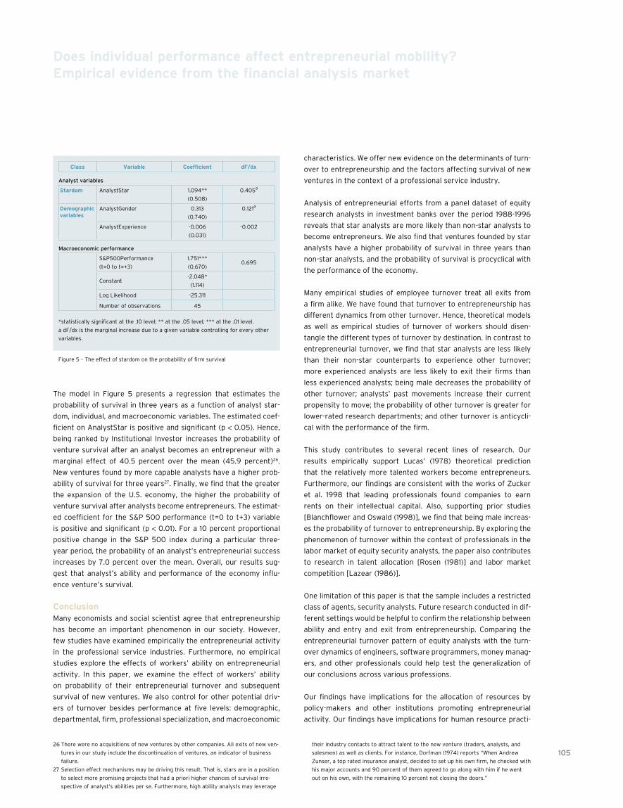
10526 There were no acquisitions of new ventures by other companies. All exits of new ven-
tures in our study include the discontinuation of ventures, an indicator of business
failure.
27 Selection effect mechanisms may be driving this result. That is, stars are in a position
to select more promising projects that had a priori higher chances of survival irre-
spective of analyst’s abilities per se. Furthermore, high ability analysts may leverage
their industry contacts to attract talent to the new venture (traders, analysts, and
salesmen) as well as clients. For instance, Dorfman (1974) reports “When Andrew
Zunser, a top rated insurance analyst, decided to set up his own firm, he checked with
his major accounts and 90 percent of them agreed to go along with him if he went
out on his own, with the remaining 10 percent not closing the doors.”
Does individual performance affect entrepreneurial mobility? Empirical evidence from the financial analysis market
The model in Figure 5 presents a regression that estimates the
probability of survival in three years as a function of analyst star-
dom, individual, and macroeconomic variables. The estimated coef-
ficient on AnalystStar is positive and significant (p < 0.05). Hence,
being ranked by Institutional Investor increases the probability of
venture survival after an analyst becomes an entrepreneur with a
marginal effect of 40.5 percent over the mean (45.9 percent)26.
New ventures found by more capable analysts have a higher prob-
ability of survival for three years27. Finally, we find that the greater
the expansion of the U.S. economy, the higher the probability of
venture survival after analysts become entrepreneurs. The estimat-
ed coefficient for the S&P 500 performance (t=0 to t+3) variable
is positive and significant (p < 0.01). For a 10 percent proportional
positive change in the S&P 500 index during a particular three-
year period, the probability of an analyst’s entrepreneurial success
increases by 7.0 percent over the mean. Overall, our results sug-
gest that analyst’s ability and performance of the economy influ-
ence venture’s survival.
conclusionMany economists and social scientist agree that entrepreneurship
has become an important phenomenon in our society. However,
few studies have examined empirically the entrepreneurial activity
in the professional service industries. Furthermore, no empirical
studies explore the effects of workers’ ability on entrepreneurial
activity. In this paper, we examine the effect of workers’ ability
on probability of their entrepreneurial turnover and subsequent
survival of new ventures. We also control for other potential driv-
ers of turnover besides performance at five levels: demographic,
departmental, firm, professional specialization, and macroeconomic
characteristics. We offer new evidence on the determinants of turn-
over to entrepreneurship and the factors affecting survival of new
ventures in the context of a professional service industry.
Analysis of entrepreneurial efforts from a panel dataset of equity
research analysts in investment banks over the period 1988-1996
reveals that star analysts are more likely than non-star analysts to
become entrepreneurs. We also find that ventures founded by star
analysts have a higher probability of survival in three years than
non-star analysts, and the probability of survival is procyclical with
the performance of the economy.
Many empirical studies of employee turnover treat all exits from
a firm alike. We have found that turnover to entrepreneurship has
different dynamics from other turnover. Hence, theoretical models
as well as empirical studies of turnover of workers should disen-
tangle the different types of turnover by destination. In contrast to
entrepreneurial turnover, we find that star analysts are less likely
than their non-star counterparts to experience other turnover;
more experienced analysts are less likely to exit their firms than
less experienced analysts; being male decreases the probability of
other turnover; analysts’ past movements increase their current
propensity to move; the probability of other turnover is greater for
lower-rated research departments; and other turnover is anticycli-
cal with the performance of the firm.
This study contributes to several recent lines of research. Our
results empirically support Lucas’ (1978) theoretical prediction
that the relatively more talented workers become entrepreneurs.
Furthermore, our findings are consistent with the works of Zucker
et al. 1998 that leading professionals found companies to earn
rents on their intellectual capital. Also, supporting prior studies
[Blanchflower and Oswald (1998)], we find that being male increas-
es the probability of turnover to entrepreneurship. By exploring the
phenomenon of turnover within the context of professionals in the
labor market of equity security analysts, the paper also contributes
to research in talent allocation [Rosen (1981)] and labor market
competition [Lazear (1986)].
One limitation of this paper is that the sample includes a restricted
class of agents, security analysts. Future research conducted in dif-
ferent settings would be helpful to confirm the relationship between
ability and entry and exit from entrepreneurship. Comparing the
entrepreneurial turnover pattern of equity analysts with the turn-
over dynamics of engineers, software programmers, money manag-
ers, and other professionals could help test the generalization of
our conclusions across various professions.
Our findings have implications for the allocation of resources by
policy-makers and other institutions promoting entrepreneurial
activity. Our findings have implications for human resource practi-
class Variable coefficient df/dx
Analyst variables
stardom AnalystStar 1.094**
(0.508)
0.405a
Demographic variables
AnalystGender 0.313
(0.740)
0.121a
AnalystExperience -0.006
(0.031)
-0.002
Macroeconomic performance
S&P500Performance
(t=0 to t=+3)
1.751***
(0.670)0.695
Constant-2.048*
(1.114)
Log Likelihood -25.311
Number of observations 45
*statistically significant at the .10 level; ** at the .05 level; *** at the .01 level.
a dF/dx is the marginal increase due to a given variable controlling for every other
variables.
Figure 5 – The effect of stardom on the probability of firm survival

106 – The journal of financial transformation
Does individual performance affect entrepreneurial mobility? Empirical evidence from the financial analysis market
tioners as well. Whereas firms try to minimize turnover to competi-
tors, at the same time, they might be maximizing entrepreneurial
turnover. To our knowledge, no study has been able to establish
what mobility is more damaging to the firm. We believe that it is an
important question for future research.
references• Blanchflower, D. G., and A. J. Oswald, 1998, “What makes an entrepreneur,” Journal of
Labor Economics, 16:1, 26-60
• Brenner, L., 1991, “The bull and the bear,” United States Banker, January, 25-27
• Burke, A. E., F. R. FitzRoy, and M. A. Nolan, 2000, “When less is more: distinguishing
between entrepreneurial choice and performance,” Oxford Bulletin of Economics &
Statistics, 62, 565-87
• Dorfman, D., 1974, “The rise of entrepreneurial analysts,” Institutional Investor, July,
43-106
• Dorfman, J., 1991, “Analysts devote more time to selling as firms keep scorecard on per-
formance,” Wall Street Journal, October 29, C1
• Dunn, T., and D. Holtz-Eakin, 2000, “Financial capital, human capital, and the transi-
tion to self-employment: evidence from intergenerational links,” Journal of Labor
Economics, 18, 282-305
• Eccles, R. G., and D. B. Crane, 1988, Doing deals, Harvard Business School, Cambridge,
MA
• Evans, D. S., and B. Jovanovic, 1989, “An estimated model of entrepreneurial choice
under liquidity constraints,” Journal of Political Economy, 97:4, 808-27
• Evans, D. S., and L. Leighton, 1989, “Some empirical aspects of entrepreneurship,” The
American Economic Review, 79, 519-35
• Foster, A., and M. Rosensweig, 1995, “Learning by doing and learning from others:
human capital and technical change in agriculture,” Journal of Political Economy, 103:6,
1176-1209
• Greene, W. H., 2000, Econometric analysis, Prentice Hall, Upper Saddle River, NJ
• Headen, A. E., 1990, “Wage, returns to ownership, and fee responses to physician sup-
ply,” The Review of Economics and Statistics, 72:1, 30-37
• Holmes, T. J., and J. A. Schmitz, 1990, “A theory of entrepreneurship and its application
to the study of business transfers,” Journal of Political Economy, 98:2, 265-94
• Holtz-Eakin, D., D. Joulfaian, and H. S. Rosen, 1994, “Entrepreneurial decisions and
liquidity constraints,” The Rand Journal of Economics, 23:2, 340-47
• Hong, H., J. D. Kubik, and A. Solomon, 2000, “Security analysts’ career concerns and
herding of earnings forecasts,” RAND Journal of Economics, 31, 121-44
• Hong, H., and J. D. Kubik, 2003, “Analyzing the analysts: career concerns and biased
earning forecasts,” The Journal of Finance, 58:1, 313-51
• Institutional Investor, 1998, “The 1998 All-America Research Team,” Institutional
Investor, October, 99-106
• Irigoyen, C., 2002, “Where do entrepreneurs come from?” Working paper, University of
Chicago
• Jovanovic, B., 1982, “Selection and the evolution of industry,” Econometrica, 50, 649-
70
• Jovanovic, B., and Y. Nyarko, 1996, “Stepping stone mobility,” NBER Working Paper
#5651
• Kihlstrom, R. E., and J. Laffont, 1979, “A general equilibrium entrepreneurial theory of
firm formation based on risk aversion,” The Journal of Political Economy, 87:4, 719-48
• King, G., and L. Zeng, 1999, “Estimating absolute, relative, and attributable risks in case-
control studies,” Department of Government, Harvard University
• King, G., and L. Zeng, 1999, “Logistic regression in rare events data,” Department of
Government Harvard University
• Knight, F., 1921, Risk, uncertainty and profit, H H, New York
• Kostigen, T., 1990, “Captain of your own ship,” Investment Dealers’ Digest, February,
22-29
• Laderman, J., 1998, “Who can you trust? Wall Street’s spin game,” Business Week,
October 5, 148-56
• Lazear, E. P., 1986. “Raids and offer matching.” Research in Labor Economics, 8A, 141-
65
• Lazear, E. P., 2002, “Entrepreneurship,” in NBER Working Paper Series 9109
• Lucas, R. E., 1978, “On the size distribution of business firms,” Bell Journal of
Economics, 9, 508-23
• Milligan, J. W., 1985, “The boutiques are making it big,” Institutional Investor, November,
175-87
• Nanda, R., and J. B. Sorensen, 2004, “Labor mobility and entrepreneurship,” Manuscript
• Pennings, J. M., K. Lee and A. van Wittelloostuijn, 1998, “Human capital, social capital
and firm dissolution,” Academy of Management Journal, 41:4, 425-40
• Phillips, B., 1997, “Free at last?” Institutional Investor, August, 48-55
• Rosen, S., 1982, “Authority, control and the distribution of earnings,” Bell Journal of
Economics, 13, 311-23
• Rosen, S., 1981, “The economics of superstars,” American Economic Review, 75, 845-58
• Schumpeter, J. A., 1934, The theory of economic development, Harvard University
Press, Cambridge, MA
• Shane, S., and T. Stuart, 2002, “Organizational endowment and the performance of uni-
versity start-ups,” Management Science, 48, 154-70
• Siconolfi, M., 1992, “Shearson research analysts finish first on ‘All -America Team’ for
third year,” The Wall Street Journal, October 13, C18
• Stickel, S. E., 1990, “Predicting individual analyst earnings forecast,” Journal of
Accounting Research, 28, 409-17
• Stickel, S. E., 1992, “Reputation and performance among security analysts,” Journal of
Finance, 47.5, 1811-36
• Watson, J., and J. E. Everett, 1993, “Defining small business failure,” International Small
Business Journal, 11:3, 35-48
• Wholey, D. R., J. B. Christianson, and S. M. Sanchez, 1993, “The effect of physician and
corporate interests on the formation of health maintenance organizations,” American
Journal of Sociology, 99:1, 164-200
• Zucker, L. G., M. R. Darby and M. B. Brewer, 1998, “Intellectual human capital and the
birth of U.S. biotechnology enterprises,” The American Economic Review, 88:1, 209-306

1071 We have benefited from comments made by seminar participants at Cass Business
School and at the 3rd Advances in Financial Economics conference (AFE), Samos,
Greece. Any remaining errors are our sole responsibility.
Part 2
A new approach for an integrated credit and market risk measurement of interest rate swap portfoliosJohn Hatgioannides
Chair in Mathematical Finance and Financial Engineering, and Director, MSc in Mathematical
Trading and Finance, Cass Business School1
George PetropoulosSenior FX Trader, EFG Eurobank
AbstractIn this paper we develop a new methodology to simultaneously
measure the credit and market risk arising from an interest rate
swap portfolio. Based on a dynamic hedging methodology, which
uses credit spread index options to hedge swap exposures, the
probability of default is embedded in the credit spread option price.
The end result is a creation of a portfolio of swaps and credit spread
options that, when rebalanced continuously, has zero default risk.
It is only the market value of such a combined portfolio that is
sensitive to both market and credit risk factors. Our approach has
important implications for the implementation of the standard
paradigm of integrated risk measurement. Most notably, since the
credit part of our combined portfolio is linked to the potential credit
exposure of the swap portfolio through its notional and the prob-
ability of default is represented by the price of the credit spread
option, we are not relying at all on the probabilities of default in
the calculation of the total expected economic loss. We empirically
illustrate our approach using an active swaps portfolio taken from
a medium-sized European bank and compare our findings with the
standard model.
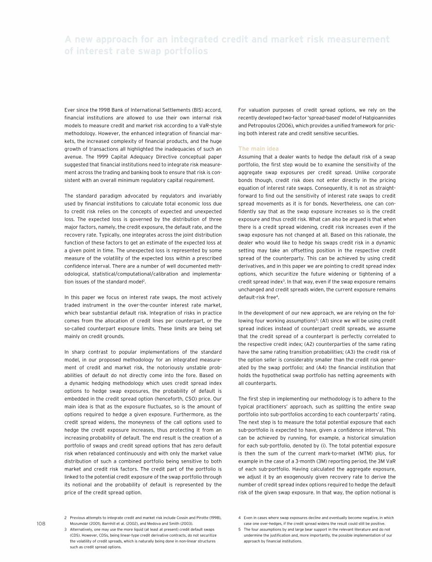
1082 Previous attempts to integrate credit and market risk include Cossin and Pirotte (1998),
Mozumdar (2001), Barnhill et al. (2002), and Medova and Smith (2003).
3 Alternatively, one may use the more liquid (at least at present) credit default swaps
(CDS). However, CDSs, being linear-type credit derivative contracts, do not securitize
the volatility of credit spreads, which is naturally being done in non-linear structures
such as credit spread options.
4 Even in cases where swap exposures decline and eventually become negative, in which
case one over-hedges, if the credit spread widens the result could still be positive.
5 The four assumptions by and large bear support in the relevant literature and do not
undermine the justification and, more importantly, the possible implementation of our
approach by financial institutions.
A new approach for an integrated credit and market risk measurement of interest rate swap portfolios
Ever since the 1998 Bank of International Settlements (BIS) accord,
financial institutions are allowed to use their own internal risk
models to measure credit and market risk according to a VaR-style
methodology. However, the enhanced integration of financial mar-
kets, the increased complexity of financial products, and the huge
growth of transactions all highlighted the inadequacies of such an
avenue. The 1999 Capital Adequacy Directive conceptual paper
suggested that financial institutions need to integrate risk measure-
ment across the trading and banking book to ensure that risk is con-
sistent with an overall minimum regulatory capital requirement.
The standard paradigm advocated by regulators and invariably
used by financial institutions to calculate total economic loss due
to credit risk relies on the concepts of expected and unexpected
loss. The expected loss is governed by the distribution of three
major factors, namely, the credit exposure, the default rate, and the
recovery rate. Typically, one integrates across the joint distribution
function of these factors to get an estimate of the expected loss at
a given point in time. The unexpected loss is represented by some
measure of the volatility of the expected loss within a prescribed
confidence interval. There are a number of well documented meth-
odological, statistical/computational/calibration and implementa-
tion issues of the standard model2.
In this paper we focus on interest rate swaps, the most actively
traded instrument in the over-the-counter interest rate market,
which bear substantial default risk. Integration of risks in practice
comes from the allocation of credit lines per counterpart, or the
so-called counterpart exposure limits. These limits are being set
mainly on credit grounds.
In sharp contrast to popular implementations of the standard
model, in our proposed methodology for an integrated measure-
ment of credit and market risk, the notoriously unstable prob-
abilities of default do not directly come into the fore. Based on
a dynamic hedging methodology which uses credit spread index
options to hedge swap exposures, the probability of default is
embedded in the credit spread option (henceforth, CSO) price. Our
main idea is that as the exposure fluctuates, so is the amount of
options required to hedge a given exposure. Furthermore, as the
credit spread widens, the moneyness of the call options used to
hedge the credit exposure increases, thus protecting it from an
increasing probability of default. The end result is the creation of a
portfolio of swaps and credit spread options that has zero default
risk when rebalanced continuously and with only the market value
distribution of such a combined portfolio being sensitive to both
market and credit risk factors. The credit part of the portfolio is
linked to the potential credit exposure of the swap portfolio through
its notional and the probability of default is represented by the
price of the credit spread option.
For valuation purposes of credit spread options, we rely on the
recently developed two-factor ‘spread-based’ model of Hatgioannides
and Petropoulos (2006), which provides a unified framework for pric-
ing both interest rate and credit sensitive securities.
The main ideaAssuming that a dealer wants to hedge the default risk of a swap
portfolio, the first step would be to examine the sensitivity of the
aggregate swap exposures per credit spread. Unlike corporate
bonds though, credit risk does not enter directly in the pricing
equation of interest rate swaps. Consequently, it is not as straight-
forward to find out the sensitivity of interest rate swaps to credit
spread movements as it is for bonds. Nevertheless, one can con-
fidently say that as the swap exposure increases so is the credit
exposure and thus credit risk. What can also be argued is that when
there is a credit spread widening, credit risk increases even if the
swap exposure has not changed at all. Based on this rationale, the
dealer who would like to hedge his swaps credit risk in a dynamic
setting may take an offsetting position in the respective credit
spread of the counterparty. This can be achieved by using credit
derivatives, and in this paper we are pointing to credit spread index
options, which securitize the future widening or tightening of a
credit spread index3. In that way, even if the swap exposure remains
unchanged and credit spreads widen, the current exposure remains
default-risk free4.
In the development of our new approach, we are relying on the fol-
lowing four working assumptions5: (A1) since we will be using credit
spread indices instead of counterpart credit spreads, we assume
that the credit spread of a counterpart is perfectly correlated to
the respective credit index; (A2) counterparties of the same rating
have the same rating transition probabilities; (A3) the credit risk of
the option seller is considerably smaller than the credit risk gener-
ated by the swap portfolio; and (A4) the financial institution that
holds the hypothetical swap portfolio has netting agreements with
all counterparts.
The first step in implementing our methodology is to adhere to the
typical practitioners’ approach, such as splitting the entire swap
portfolio into sub-portfolios according to each counterparts’ rating.
The next step is to measure the total potential exposure that each
sub-portfolio is expected to have, given a confidence interval. This
can be achieved by running, for example, a historical simulation
for each sub-portfolio, denoted by (i). The total potential exposure
is then the sum of the current mark-to-market (MTM) plus, for
example in the case of a 3-month (3M) reporting period, the 3M VaR
of each sub-portfolio. Having calculated the aggregate exposure,
we adjust it by an exogenously given recovery rate to derive the
number of credit spread index options required to hedge the default
risk of the given swap exposure. In that way, the option notional is

109
A new approach for an integrated credit and market risk measurement of interest rate swap portfolios
linked to the total swap exposure of the portfolio over the 3-month
reporting period. In short,
SwapMTMi + SwapVaR(3M)i = Total potential exposure (3M); Option
notional = Total potential exposure (3M) ÷ 3M Credit spread index
option price (2.1)
The maturity of the credit spread index (underlying asset) and the
strike price of the option are two important parameters in imple-
menting our methodology. We propose that the maturity of the
underlying index is matched, as closely as possible, with the matu-
rity of the biggest swap exposure in each of the sub-portfolios.
The strike of the option is a parameter which greatly affects both
the cost of hedging and the diversification of credit risk. Since cred-
it spreads may be deemed as mean-reverting quantities [Pedrosa
and Roll (1998), Hatgioannides and Petropoulos (2006)], the strike
of the option should be closely related to the long-term mean of the
credit spread index. In that way, the option will be out-of-the-money
if credit spreads are low and in-the-money if credit spreads are
high, reflecting the level of risk in credit markets. In other words,
our technique creates a combined portfolio of swaps and credit
spread index options. The market value of such a portfolio is essen-
tially affected by changes in market rates (market risk) and the
levels of the credit spread (credit risk). The key result is that if one
runs a historical simulation VaR on that portfolio then an integrated
measure of risk can be readily obtained:
Integrated VaRi = Market VaRi of Swaps + Market VaRi of CSOs
(2.2)
i = counterpart rating
The first term of the above expression represents the ‘predicted’
P/L of the swap portfolio of rating (i) due to market risk. The second
term represents the amount of default risk that the specific swap
exposure runs.
The calculation of economic capitalEconomic capital represents the amount that needs to be set aside
as a provision for the credit risk exposures created by financial
securities either in the banking or the trading book.
The standard approachThere are two measures that are typically employed by financial
institutions to calculate the total economic loss due to credit risk, the
expected loss and the unexpected loss. The expected loss (EL), at a
given point in time, is given by the joint distribution of three key vari-
ables, the credit exposure, the default rate, and the recovery rate:
EL = ∫∫∫ (CE)(PrDef)(1-RR)F(CE, PrDef, RR)dCE dPrDef dRR (3.1)
where, CE is the credit exposure, PrDef stands for default rate, RR
is the recovery rate, and F(CE,PrDef,RR) is the multivariate prob-
ability function of the three variables. Assuming statistical indepen-
dence between CE, PrDE and RR, a very questionable assumption
we have to say but nevertheless widely adopted in practice to arrive
at a manageable specification, we obtain for a single exposure: EL =
E(CE) * (1-RR) * Pr[Def(ti, ti+1)] (3.2)
Similarly, the unexpected loss(UL) for a binomial event of a single
exposure is given by:
UL = ECE * (1-RR) * √(Pr[Def(ti, ti+1)](1-Pr[Def(ti, ti+1)])) (3.3)
which represents the volatility of the expected loss at a given con-
fidence interval.
The integrated approachIn our vision for the calculation of economic capital, the major
difference to current practices is that we do not explicitly rely
on default probabilities. Instead, by adopting a dynamic hedging
methodology, which uses credit spread index options to hedge
swap exposures, the probability of default is embedded in the credit
spread option price.
The intuition is that as the exposure fluctuates, so is the amount of
options required to hedge it [see expression (2.1)]. Also, as the cred-
it spread widens, the moneyness of the call options used to hedge
the credit exposure increases, acting as a shield for an increasing
probability of default. The end result is the creation of a portfolio of
swaps and credit spread options which, when rebalanced continu-
ously, has zero default risk. Crucially, the market value distribution
of that combined portfolio is sensitive to both market and credit
risk factors.
The economic capital calculation for such a portfolio then becomes
the sum of the expected and unexpected loss due to the credit part
of the portfolio. This follows from the fact that the credit part of
the portfolio is linked to the potential credit exposure of the swap
portfolio through its notional and the probability of default is rep-
resented by the price of the credit spread option.
The process of using credit spread options in order to ‘replace’ eco-
nomic loss of a swap sub-portfolio turns out to be quite appealing.
By running a historical simulation to the credit part of the portfolio,
the expected loss (EL) of the swap sub-portfolio equates to the
mean of the resulting distribution and the unexpected loss (UL) to
its standard deviation:
EL = mean of MTM of credit spread index option; UL = Standard
deviation of MTM of credit spread index option (3.4)

110
A new approach for an integrated credit and market risk measurement of interest rate swap portfolios
6 According to BIS 1998 banks can use only approved internal rating systems for all their
customers if and only if they have approved risk management systems. This is done
mainly to maintain consistency in the way that each bank calculates the credit risk of
their portfolios.
7 Information about the actual dataset and the chosen value date is available upon
request.
8 Typically, value date is defined as the date at which over-the-counter (OTC) deals are
being settled in each currency. For the EUR currency, the value date is t+2.
9 An exposure with negative MTM is termed as wrong-way exposure. Not accounting in
this study for such exposures does not mean that we disregard them completely. It just
happens that the total expected credit exposure after 3 months (our chosen reporting
period) is still negative.
10 We have also extensively experimented with multi-step Monte Carlo simulations of the
swap sub-portfolios for both our approach and the standard one. The results do not
considerably differ.
11 Analytic calculations are available upon request.
In this way, the modeling of the probabilities of default is being
done through the same analytic framework used to price both
swaps and credit spread options, ensuring internal consistency in
the operations of the financial institution.
An empirical illustrationThe interest rate swap portfolio
An actual swap portfolio was provided by a medium-sized European
bank with a substantial business in the euro (EUR) swap markets.
The swap portfolio contains 53 vanilla interest rate swaps denomi-
nated in euros. Overall, the portfolio is short, which means that if
rates move down the portfolio makes money and vice versa. The
portfolio contains deals with various European and U.S. counter-
parts of different ratings. Although the bank in question has an
approved internal rating system6, for the purposes of this paper, we
have decided to use the S&P long-term ratings in order to rate each
swap deal according to the rating of the counterpart.
In total, there are 15 different counterparts with 7 different ratings.
They are all rated at the investment grade spectrum, i.e., AAA, AA,
AA-, A+, A, A- and BBB+. The medium-sized European bank has
netting agreements with all the counterparts in the portfolio (in
accordance with Assumption A4 above). This is important because
we can sum up all the exposures per counterpart.
The swap exposures were grouped per counterpart rating to create
the 7 sub-portfolios7. This aggregation was based on the assump-
tion that counterparts of the same rating follow the same default
process (in accordance with Assumption A2 above). The portfolio
consists of deals in EUR currency only, mainly with European coun-
terparts. Hence, for our subsequent hedging purposes we only use
European credit spread indices.
The market risk per sub-portfolio, in terms of a parallel yield curve
shift of one basis point (bp), differs across the sub-portfolios, as
expected. Generally speaking, if interest rates move upwards in
the Euro Area, then most of the sub-portfolios will lose money. In
contrast, the credit exposure of these portfolios will be reduced
since the actual credit exposure is defined as the maximum of zero
and a positive mark-to-market at an arbitrary point in time t, where
t is equal to the value date8. Given the proprietary nature of the
dataset, we have chosen not to report here the actual date of our
calculations. The sub-portfolios created following the grouping of
the exposures are shown in Figure 1. It is obvious that only 4 out
of the 7 sub-portfolios exhibit positive exposure. The other 3 have
zero exposure since their current mark-to-market is negative9.
The integrated measure
The market and credit risk for each of the 4 sub-portfolios with
positive exposure were calculated using expression (2.2) by run-
ning a historical simulation10 -based VaR on weekly data covering
the 2 years prior to the value/reference date. The time horizon is
3 months and the confidence interval is set at 99%. It is evident
from expression (2.1) that one has to decide on the maturities of the
underlying credit spread indices, set the strike prices of the credit
spread call index options, and calculate their prices before finding
the option notional.
We make use of the credit spread option valuation model and
calibration approach developed by Hatgioannides and Petropoulos
(2006). Since our AAA, A-, BBB+ swap sub-portfolios have all matur-
ities of 2 years and the AA sub-portfolio has a maturity of 9 years,
we have collected 2 years’ worth of data on AAA, AA, A-, BBB+
credit spread indices that match the expirations of the correspond-
ing sub-portfolios, calculate their long run mean, set the strikes of
the credit spread options equal to the corresponding index’s long
run mean, and find the 4 credit spread index options price11. Results,
together with the swaps VaR, credit spread index options VaR, and
our measure of integrated VaR are all shown in Figure 2.
It is obvious from Figure 2 that the integrated measure is higher
than the swaps’ market VaR alone, showing that there is no diversi-
fication effect since the two sources of risk are not directly linked.
The ratio of the credit spread index options VaR and the integrated
VaR reported in the last line of Figure 2 shows the level of default
risk that each sub-portfolio runs. This figure is crucial for the risk
manager. For example for the A- sub-portfolio the ratio is as high
as 47%, indicating an increased default risk arising from the swap
exposure profile and the level of the credit spread index. Based
on these ratios, a risk manager could readily set limits and trigger
sub-portfolio no. s+P rating long/short currency Actual credit exposure
1 AAA Short EUR 276,664
2 AA Short EUR 3,452,793
3 AA- Short EUR -2,490,101
4 A+ Short EUR -1,478,964
5 A Short EUR -1,152,408
6 A- Short EUR 1,017,100
7 BBB+ Short EUR 972,223
2Y AAA 9Y AA 2Y A- 2Y BBB+
Option strike (bp) 28 56 78 81
Option price (decimals) 3M 0.583 0.489 0.601 0.682
Swaps VaR 260,792 1,848,815 76,641 102,812
Credit spread index options VaR 10,776 28,518 68,781 27,804
Integrated VaR 271,568 1,877,333 145,422 130,616
Ratio 4% 2% 47% 21%
Figure 1 – Credit exposure of sub-portfolios
Figure 2 – Integrated VaR per sub-portfolio
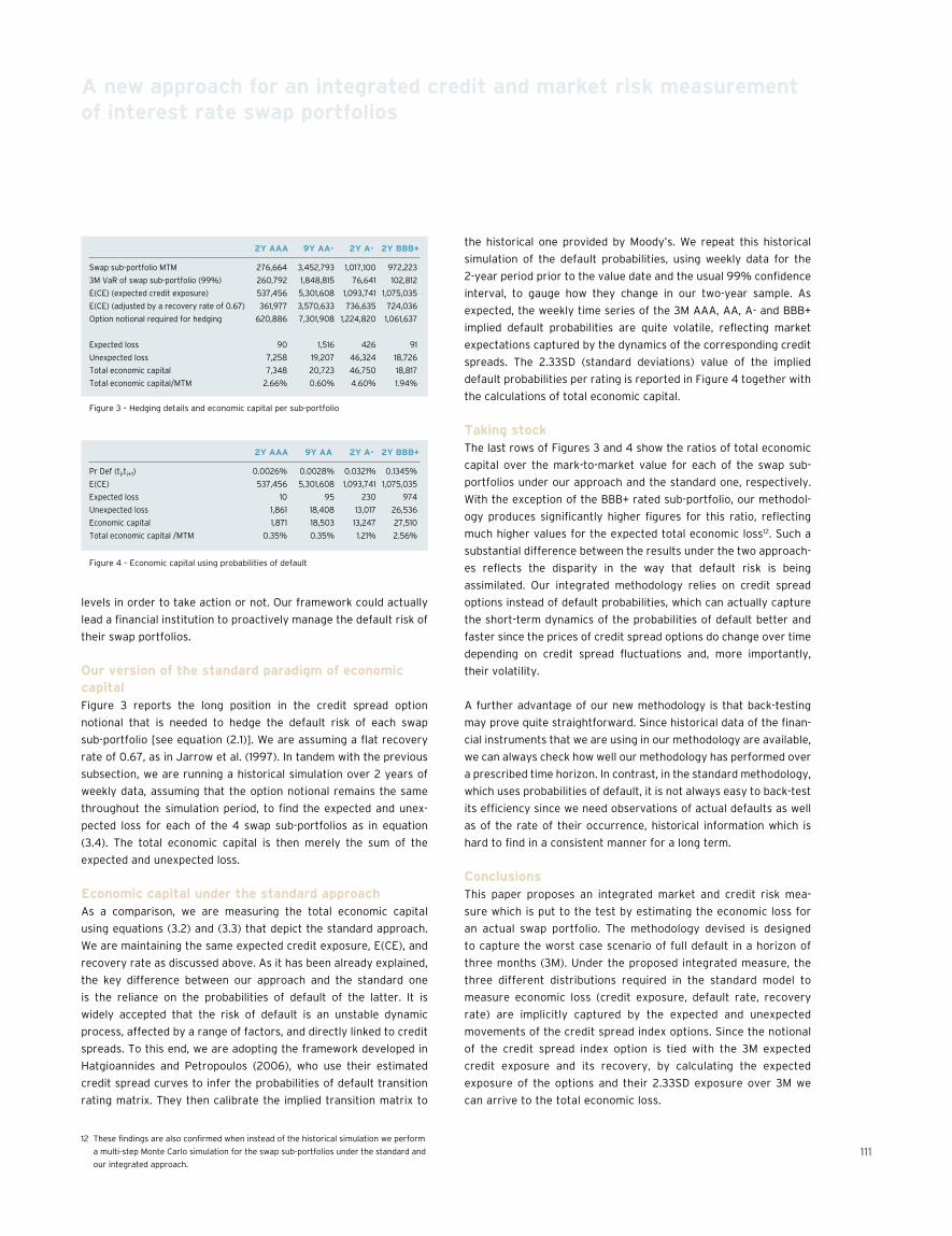
11112 These findings are also confirmed when instead of the historical simulation we perform
a multi-step Monte Carlo simulation for the swap sub-portfolios under the standard and
our integrated approach.
A new approach for an integrated credit and market risk measurement of interest rate swap portfolios
levels in order to take action or not. Our framework could actually
lead a financial institution to proactively manage the default risk of
their swap portfolios.
our version of the standard paradigm of economic capitalFigure 3 reports the long position in the credit spread option
notional that is needed to hedge the default risk of each swap
sub-portfolio [see equation (2.1)]. We are assuming a flat recovery
rate of 0.67, as in Jarrow et al. (1997). In tandem with the previous
subsection, we are running a historical simulation over 2 years of
weekly data, assuming that the option notional remains the same
throughout the simulation period, to find the expected and unex-
pected loss for each of the 4 swap sub-portfolios as in equation
(3.4). The total economic capital is then merely the sum of the
expected and unexpected loss.
Economic capital under the standard approachAs a comparison, we are measuring the total economic capital
using equations (3.2) and (3.3) that depict the standard approach.
We are maintaining the same expected credit exposure, E(CE), and
recovery rate as discussed above. As it has been already explained,
the key difference between our approach and the standard one
is the reliance on the probabilities of default of the latter. It is
widely accepted that the risk of default is an unstable dynamic
process, affected by a range of factors, and directly linked to credit
spreads. To this end, we are adopting the framework developed in
Hatgioannides and Petropoulos (2006), who use their estimated
credit spread curves to infer the probabilities of default transition
rating matrix. They then calibrate the implied transition matrix to
the historical one provided by Moody’s. We repeat this historical
simulation of the default probabilities, using weekly data for the
2-year period prior to the value date and the usual 99% confidence
interval, to gauge how they change in our two-year sample. As
expected, the weekly time series of the 3M AAA, AA, A- and BBB+
implied default probabilities are quite volatile, reflecting market
expectations captured by the dynamics of the corresponding credit
spreads. The 2.33SD (standard deviations) value of the implied
default probabilities per rating is reported in Figure 4 together with
the calculations of total economic capital.
Taking stockThe last rows of Figures 3 and 4 show the ratios of total economic
capital over the mark-to-market value for each of the swap sub-
portfolios under our approach and the standard one, respectively.
With the exception of the BBB+ rated sub-portfolio, our methodol-
ogy produces significantly higher figures for this ratio, reflecting
much higher values for the expected total economic loss12. Such a
substantial difference between the results under the two approach-
es reflects the disparity in the way that default risk is being
assimilated. Our integrated methodology relies on credit spread
options instead of default probabilities, which can actually capture
the short-term dynamics of the probabilities of default better and
faster since the prices of credit spread options do change over time
depending on credit spread fluctuations and, more importantly,
their volatility.
A further advantage of our new methodology is that back-testing
may prove quite straightforward. Since historical data of the finan-
cial instruments that we are using in our methodology are available,
we can always check how well our methodology has performed over
a prescribed time horizon. In contrast, in the standard methodology,
which uses probabilities of default, it is not always easy to back-test
its efficiency since we need observations of actual defaults as well
as of the rate of their occurrence, historical information which is
hard to find in a consistent manner for a long term.
conclusionsThis paper proposes an integrated market and credit risk mea-
sure which is put to the test by estimating the economic loss for
an actual swap portfolio. The methodology devised is designed
to capture the worst case scenario of full default in a horizon of
three months (3M). Under the proposed integrated measure, the
three different distributions required in the standard model to
measure economic loss (credit exposure, default rate, recovery
rate) are implicitly captured by the expected and unexpected
movements of the credit spread index options. Since the notional
of the credit spread index option is tied with the 3M expected
credit exposure and its recovery, by calculating the expected
exposure of the options and their 2.33SD exposure over 3M we
can arrive to the total economic loss.
2Y AAA 9Y AA- 2Y A- 2Y BBB+
Swap sub-portfolio MTM 276,664 3,452,793 1,017,100 972,223
3M VaR of swap sub-portfolio (99%) 260,792 1,848,815 76,641 102,812
E(CE) (expected credit exposure) 537,456 5,301,608 1,093,741 1,075,035
E(CE) (adjusted by a recovery rate of 0.67) 361,977 3,570,633 736,635 724,036
Option notional required for hedging 620,886 7,301,908 1,224,820 1,061,637
Expected loss 90 1,516 426 91
Unexpected loss 7,258 19,207 46,324 18,726
Total economic capital 7,348 20,723 46,750 18,817
Total economic capital/MTM 2.66% 0.60% 4.60% 1.94%
2Y AAA 9Y AA 2Y A- 2Y BBB+
Pr Def (ti,ti+1) 0.0026% 0.0028% 0.0321% 0.1345%
E(CE) 537,456 5,301,608 1,093,741 1,075,035
Expected loss 10 95 230 974
Unexpected loss 1,861 18,408 13,017 26,536
Economic capital 1,871 18,503 13,247 27,510
Total economic capital /MTM 0.35% 0.35% 1.21% 2.56%
Figure 3 – Hedging details and economic capital per sub-portfolio
Figure 4 – Economic capital using probabilities of default

112 – The journal of financial transformation
A new approach for an integrated credit and market risk measurement of interest rate swap portfolios
The comparison between the standard paradigm and our integrated
approach proved to be quite interesting. Although financial manag-
ers might not subscribe to the lower return on capital that, in view of
our results our integrated approach entails, the road to the current
financial crisis and its enduring adverse effects necessitate enhanced
prudence and increased solvency of financial operations.
references• Barnhill M. T., P. Papanagiotou, and L. Schmacher, 2002, “Measuring integrated market
and credit risk in bank portfolios: an application to a set of hypothetical banks operat-
ing in South Africa,” Financial Markets, Institutions & Instruments, 11:5, 401-443
• Basle Committee on Banking Supervision, 1999, Credit risk modelling: current practices
and applications
• Basle Committee on Banking Supervision, 2001, The new Basel capital accord
• British Bankers Association, 1999, Credit risk and regulation panel
• Cossin, D., and H. Pirotte, 1998, “How well do classical credit risk pricing models fit
swap transaction data?” European Financial Management, 4, 65 – 78
• Hatgioannides, J., and G. Petropoulos, 2006, “On credit spreads, cresit spread options
and implied probabilities of default,” mimeo, Cass Business School
• Jarrow, R., D. Lando, and S. Turnbull, 1997, “A Markov model for the term structure of
credit spreads,” Review of Financial Studies, 10, 481-523
• Medova, E. A., and R. G. Smith, 2003, “A framework to measure integrated risk,” Euro
Working Group on Financial Modelling 32nd Meeting, London
• Mozumdar, A., 2001, “Corporate hedging and speculative incentives: implications for
swap market defualt risk,” Journal of Financial and Quantitative Analysis, 36:2, 221-250
• Pedrosa, M., and R. Roll, 1998, “Systematic risk in corporate bond credit spreads,”
Journal of Fixed Income, December, 7 – 26

113
risk drivers in historical simulation: scaled percentage changes versus first differences1
su XuVice President, Risk Analytics, Wachovia Securities
stephen D. YoungSenior Vice President and Director of the Options
Strategy Group, Evergreen Investments
AbstractWith historical simulation it is often asserted that the calculation
of value-at-risk (VaR) under this approach is based simply on using
time series of historical data and changes which actually occurred
to estimate risk. This paper examines two distinct measurements
of change which include a simple first difference and a percent-
age change which is scaled by the current value of the relevant
risk factor. While the two measurements of change are both used
in industry, we know of no discussion regarding a comparison
of the two measurements and when to use one versus another.
While it may be widely believed that the two measurements gener-
ate similar VaR numbers, this investigation reveals that the two
measurements generate quite different values for volatile markets
and produce similar estimates for more normal environments.
Backtesting in this paper demonstrates that the first difference
is superior to the scaled percentage for risk drivers which exhibit
Part 2
1 We would like to thank Dr. George Jabbour of The George Washington University,
Marat Kramin of Wachovia Securities, and Ping Hu and Seyi Olurotimi of Evergreen
Investments for their helpful comments. The views expressed in this article are those
of the authors and do not necessarily reflect the position of Wachovia Securities or
Evergreen Investments.
mean-reversion, such as interest rates and CDS spreads, while the
scaled percentage appears superior for the equity risk drivers. One
downside for first differences is that the measurement of change
does not preclude negative risk driver values, which for this metric
we observe for short-term interest rates and CDS spreads. Firms
should be interested in this research as we show that VaR values
based on these two distinct changes may be very different and that
this would impact capital requirements. In this work we show that
it is only with exploration that practitioners may be able to choose
an appropriate metric for a particular risk factor while this is often
taken for granted in describing and implementing the historical
simulation method for VaR. Thus this paper has a very real-world
orientation with practical implications that managers and risk pro-
fessionals should find interesting.

114 – The journal of financial transformation
Historical simulation represents one approach to calculate VaR
where the thrust of the approach is that the joint distribution of
returns to an asset or portfolio may be reasonably approximated by
the past joint return distribution. Thus historical simulation involves
using past data in a very direct way where it is a guide as to what
may happen in the future. There are well known issues with histori-
cal simulation as there are with any risk measurement methodol-
ogy. We will not dwell on them here except to state that the most
glaringly obvious is the length of data to employ and the lack of
long time series for certain risk factors. In addition and more gener-
ally, VaR only seeks to measure the likelihood of a particular loss
but not the magnitude given a move beyond the specified threshold,
which is the focus of conditional VaR (CVaR) — also referred to as
expected shortfall (ES) or expected tail loss (ETL). There are inher-
ent benefits to the historical simulation approach which include not
having to estimate large correlation or covariance matrices and
that the method is non-parametric and may capture certain styl-
ized facets of the data which may not be adequately modeled via
a parametric approach. Contrary to popular belief the approach is
not ‘assumption free’ as one must make assumptions regarding the
length of time series, the underlying risk factors, portfolio holdings,
and even the definition of the changes in the underlying data.
With historical simulation there are two main approaches to calculat-
ing profit and loss, which include the full revaluation of all financial
instruments and a simple sensitivity-based approach where for non-
linear instruments it is typically the so-called delta-gamma method.
The former approach takes forecasted risk factors from the histori-
cal simulation method as inputs to a valuation model to fully revalue
all positions. The latter valuation approach is based on using sensitiv-
ity measures from pricing models coupled with the forecasted risk
factors from the historical simulation to revalue positions.
Risk factors or drivers speak to those variables of interest which
would impact the value of specified underlying financial instruments.
Risk factors include random variables such as stock prices, interest
rates, foreign exchange spot rates, commodity prices, credit spreads,
and so on. The main premise of historical simulation is that we can
measure the risk of our portfolio by using past changes to risk factors
to revalue our financial instruments using today’s set, as the stan-
dard assumption is that the portfolio is held constant. Consequently,
with the historical simulation method one simply assumes that the
distribution of tomorrow’s portfolio returns may be well approxi-
mated by the empirical distribution of past changes.
There have been enhancements proposed to the basic histori-
cal simulation approach including, but not limited to, weighting
schemes as proposed by Boudoukh et al. (1998) and volatility
updating as described by Hull and White (1998). In any event, the
fundamental premise of the approach, which is that historical
changes can be used to revalue today’s portfolio and to calculate a
percentile loss for tomorrow or beyond, still remains the same.
In this paper we focus on the measurement of changes in the under-
lying risk factors. While some authors specifically define this mea-
surement others simply mention that, with historical simulation,
one uses time series of past data to calculate changes to today’s
portfolio value at some specified percentile over a particular time
horizon. Without exhausting the list of authors we simply mention
that Hull (2002) explicitly refers to returns as percentage changes,
Jorion (2007) simply mentions returns, and Finger (2006) poses
the question what “do we mean by price changes? Should we apply
absolute differences or returns?” That is, should one use first dif-
ferences or percentage changes?
Herein we examine two distinct measurements which include a
standard scaled percentage change and a first difference. Using
time series of data and each of these metrics, we examine risk fac-
tor changes calculated over a wide array of variables which span
various markets. Based on standard backtesting at a specified
percentile, we determine which metric is statistically more robust
for each of the drivers over the entire data sample. We test the two
distinct changes (i.e., standard percentage change scaled by the
current value of the relevant risk factor and first difference) for
accuracy based on the number of expected violations (i.e., failures)
and measure the statistical efficacy of the backtesting. Further, we
examine the pattern of violations and look for ‘clustering’ or ‘bunch-
ing’ in the data and formally test for independence with respect to
violations and jointly for independence and coverage of violations
via a conditional coverage likelihood ratio. Finally, we go beyond
what has become the standard statistical testing to explore other
issues such as negativity of the underlying risk factors and the dif-
ference in VaR as calculated using one metric versus the other.
Historical simulation methodGiven time series of risk factors, historical simulation seeks to
estimate a measure of VaR that is based on revaluation which
is either model driven (i.e., full re-valuation) or from a truncated
Taylor Series to the second order (i.e., delta-gamma approach). A
risk factor (or driver) is an input variable that can affect the value
of a financial instrument, derivative or otherwise. With historical
simulation one uses the percentage change or first difference in
risk factor values observed between time periods ti and ti-Δ, where
Δ>0. Thus, with historical simulation one takes a time series of data
for some number of trading days for a particular risk factor denoted
as ƒii = 1,n, where n is somewhat arbitrary but with a minimum of
250 days for regulatory reporting as per the Basle Committee on
Banking Supervision (2005). Today’s value of the risk factor may
be denoted as ƒtoday. If one can estimate tomorrow’s value of a
particular risk factor ƒtomorrow, then one may revalue a financial
instrument whose value is a function of this risk factor and perhaps
others.
risk drivers in historical simulation: scaled percentage changes versus first differences

115
To estimate tomorrow’s value of a risk factor one must make an
assumption in the historical simulation. One popular assumption
is that the percentage change of a risk factor between today and
tomorrow is the same as it was between time periods i and i-Δ. If
we are calculating VaR over a one-day horizon (Δ = 1) then we can
write that: ƒtomorrow / ƒtoday = ƒi / ƒi-1 (1) or ƒtomorrow = ƒtoday · ƒi /
ƒi-1 (2).
From equation (2) it can be shown that: ƒtomorrow – ƒtoday = ƒtoday ·
(ƒi – ƒi-1)/ ƒi-1 (3)
The full revaluation approach is based on equation (2), as one
obtains a value for the relevant risk factor and simply uses it as an
input to a pricing model or more directly for a linear instrument. In
contrast, equation (3) is used for the delta-gamma approximation
as it defines a change. Under the delta-gamma approach the change
in value (ΔP) of a position (P) is given by:
ΔP ≈ Σk→ ∂P/∂ƒk · Δƒk + ½Σk→ ∂2P/∂ƒ2k · (Δƒk)2 (4), where the sum-
mations are taken over all underlying risk factors and sensitivities
(i.e., there are k risk factors with ∂P/∂ƒk and ∂2P/∂ƒ2k for each and
a time series of values for each risk factor), which are commonly
referred to as the delta and gamma values respectively. For many
financial instruments these partial derivatives are typically calcu-
lated based on a differencing scheme where one may use the fol-
lowing: ∂P/∂ƒk ≈ [P(ƒk + δk) – P(ƒk – δk)] ÷ 2δk (5).
∂2P/∂ƒ2k ≈ [P(ƒk + δk) – 2P(ƒk) + P(ƒk – δk)] ÷ δ2
k (6), where δk is a
small change to single risk factor ƒk at a particular point in time.
Given these approximations and one year of trading data (i.e.,
approximately 252 observations), for each risk factor Δƒ = ƒtomorrow
– ƒtoday is determined by equation (3) for all 251 possible changes
(i.e., ΔP1, ΔP2, ···, ΔP251, which are determined using equation (4) or
full revaluation). It is important to note that the time series need
not be simply one year and that the length of time between risk
factor changes may be greater than one day.
Equations (1) and (3) state that the scaled percentage change or
return between tomorrow and today (or over a longer length of
time) is the same as they were between days i and i-1. This is the
crux of the basic historical simulation method and we can define
the below as a percentage change or return based assumption:
(ƒtomorrow – ƒtoday)/ƒtoday = (ƒi – ƒi-1)/ƒi-1 (7).
Relative to the above, often financial institutions will use a simple
first difference with historical simulation to forecast risk factor
changes for random variables such as interest rates, bond spreads,
credit default swap spreads (CDS), etc. With this approach changes
in risk factors are given by: ƒtomorrow – ƒtoday = ƒi – ƒi-1 (8).
We define equations (7) and (8) as the percentage change and first
difference assumptions respectively, where we note that the length
of the difference is set equal to one trading day but this need not
be the case.
In general, returns to financial instruments are often measured in
log-space, which fits neatly with the concept of limited liability for
equity shares and the non-negativity of many financial variables.
And, with the standard Monte-Carlo method, one typically works
with log returns for simulation in the real or risk-neutral measure
(i.e., for VaR or for derivatives valuation respectfully). That said,
the difference between the standard percentage change and log-
returns are typically negligible for high-frequency data as the
ln(1+x) →x for small values of x. When one attempts to forecast risk
drivers in historical simulation using log-returns or scaled percent-
age changes is equivalent. It seems widely agreed upon to model
equity share changes using the scaled percentage change based
assumption (i.e., or log-return data) but this point is not as settled
as it pertains to other risk factors such as interest rates and credit
spreads especially over short time horizons. Just as one may use
the standard Geometric Brownian Motion model to generate future
values of stock or index prices, interest rates and credit spreads are
often modeled using a mean-reverting stochastic process where
the variable of interest is assumed normally distributed which may
result in negative values.
As discussed previously, we have as our two measures of change
the following: ƒtomorrow – ƒtoday = ƒtoday (ƒi – ƒi-1)/ ƒi-1 (9) and
ƒtomorrow – ƒtoday = ƒi – ƒi-1 (10), which are the scaled percentage
change and first difference metrics respectively. Compared to the
right hand side of equation (10), which is a straightforward differ-
ence between times ti and ti-1, the right hand side of equation (9)
has a scaling term as each ƒi – ƒi-1 is multiplied by a factor of ƒtoday/
ƒi-1. It is this factor which leads to the potential differences in the
P&L and VaR values where for larger relative differences between
today’s value of a respective factor and the value at time ti-1 the
greater the difference between the two metrics.
AnalysisThe Basle Committee on Banking Supervision (2005) requires that
if one adopts an internal model based approach to calculate VaR
then backtesting must be carried out regularly. In this section we
briefly define VaR, then we describe the relevant risk factors (i.e.,
the data), we detail the testing methods which we apply, and, finally,
we present our testing results.
VaR is a loss level over a particular horizon, with a specified confi-
dence level, that one believes will not be exceeded. We denote this
loss measure as VaR(k, α), where α is the critical value which cor-
responds to the percentile of the respective risk factor distribution
such that the probability for VaR(k, α) is consistent with α and the
loss measure is conditional on information up to the time period
of measurement. In measuring VaR(k, α) we use changes given by
risk drivers in historical simulation: scaled percentage changes versus first differences

116 – The journal of financial transformation
risk drivers in historical simulation: scaled percentage changes versus first differences
each of equations (9) and (10), which is the crux of our analysis as
we seek to explore the difference in VaR estimates associated with
using these two change metrics. For financial institutions that use
an internal models-based approach it is a requirement that one
tests the VaR model for failures or violations. That is, given a time
series of data (i.e., risk factors, instrument values, or changes in
P&L), one counts the number of days in the sample and defines
the failure rate to be the number of incidents where the variable
of interest was worse than expected given the specification of the
VaR measure. In measuring VaR, we go directly to the risk factors
and do not seek to measure instrument or portfolio level metrics
as we are concerned with simply the measurement of the changes
in these primary factors which serve to facilitate the valuation of
instruments and aggregate portfolios via an appropriate method.
The confidence level of a VaR estimate is given by p = (1 – α) and it
is convention to report VaR as a positive value, which means that
we take the negative of the loss measure. Given that the confidence
level is p = (1 – α) then with a good VaR model over time one should
observe the number of changes in risk factor values which exceed
the confidence level α-percent of the time. If one specifies a con-
fidence level of 99% then given a sample of risk factor data one
should observe changes which exceed this level 1% of the time. A
model that does not meet backtesting standards results in a penalty
(i.e., an increase in the scalar used to determine capital require-
ments from the regulatory specified base level of three).
The Basle Committee on Banking Supervision (2005) requires that
banks calculate VaR on a daily basis, utilize a confidence level of
99%, and a forecast horizon of 10-days. The historical dataset
to be used to determine model inputs, or directly for historical
simulation, must include at least 250 trading days. In many cases
financial institutions simply compute 1-day VaR and then scale the
measure by the square-root-of time (i.e., √10 which is the factor to
move from one to ten days), where this is appropriate if returns
are independently distributed. Adjustments may be made to take
dependence into account when scaling from one to ten days. It
is curious that many who use historical simulation using 1-day
changes scale the VaR measure by the square root of time to get
a 10-day VaR value. This scaling is only appropriate if the variance
is proportional to time which is consistent with the assumption
of normality but the historical simulation method seeks to avoid
parametric assumptions. In practice this simple scaling is routinely
done as calculating VaR using 10-day changes would require a
larger amount of data.
In the analysis in this paper we examine directly the changes in
various risk factors at a 99% confidence level, over a 1-day horizon,
using 252 trading days of data and rolling periods. A list of risk fac-
tors, descriptions, start and end dates, and number of observations
is included in Figure 1. As is clear, we have factors which span vari-
ous markets (i.e., fixed income, foreign exchange, equity, commod-
ity, and credit) which allows for a rich analysis.
The statistical tests which we employ include those proposed by
Kupiec (1995) and Christoffersen (1998) and further detailed in
Christoffersen (2003) which we largely follow in this section. In
implementing the likelihood ratio test proposed by Kupiec (1995),
we observe a time series of ex-ante VaR forecasts and past ex-post
returns and form a failure or hit sequence of VaR violations by
defining a simple indicator variable It+k as follows:
It+k = 1, if ƒi – ƒi-1 ≤ VaR(k,α); 0, if ƒi – ƒi-1 > VaR(k,α) (11), where
k=1 for our analysis, ƒi – ƒi-1 represents actual daily changes for a
particular risk factor for i = 1,251 , and, for comparison, VaR(k,α)
is measured using two change metrics (i.e., based on equations
risk factor start date End date # of observations
Panel A — Interest rates
6 month USD rate 04/01/1993 30/06/2008 4,033
2 year USD rate 04/01/1993 30/06/2008 4,033
5 year USD rate 04/01/1993 30/06/2008 4,033
10 year USD rate 04/01/1993 30/06/2008 4,033
6 month JPY rate 04/01/1993 30/06/2008 3,629
2 year JPY rate 04/01/1993 30/06/2008 3,629
5 year JPY rate 04/01/1993 30/06/2008 3,629
10 year JPY rate 04/01/1993 30/06/2008 3,629
Generic corporate BBB 6 month USD rate 01/01/1996 30/06/2008 3,259
Generic corporate BBB 2 year USD rate 01/01/1996 30/06/2008 3,259
Generic corporate BBB 5 year USD rate 01/01/1996 30/06/2008 3,259
Generic corporate BBB 10 year USD rate 01/01/1996 30/06/2008 3,259
Generic corporate BB 6 month USD rate 01/01/1996 30/06/2008 3,259
Generic corporate BB 2 year USD rate 01/01/1996 30/06/2008 3,259
Generic corporate BB 5 year USD rate 01/01/1996 30/06/2008 3,259
Generic corporate BB 10 year USD rate 01/01/1996 30/06/2008 3,259
Panel B — foreign exchange rates
USD/JPY FX rate 01/01/1993 30/06/2008 4,042
USD/GBP FX rate 01/01/1993 30/06/2008 4,042
USD/EUR FX rate 31/12/1998 30/06/2008 2,478
Panel c — Equity
S&P 500 index 04/01/1993 30/06/2008 3,903
IBM Corporation 04/01/1993 30/06/2008 3,903
Amazon.com Inc. 15/05/1997 30/06/2008 2,799
VIX index 04/01/1993 30/06/2008 3,903
Panel D — commodities
1 month crude oil 04/01/1993 30/06/2008 3,881
1 month natural gas 04/01/1993 30/06/2008 3,881
Panel E — Generic credit default swap spreads
Generic Corporate BBB 6 month CDS 01/01/2003 30/06/2008 1,433
Generic Corporate BBB 3 year CDS 01/01/2003 30/06/2008 1,433
Generic Corporate BBB 5 year CDS 01/01/2003 30/06/2008 1,433
Generic Corporate BBB 10 year CDS 01/01/2003 30/06/2008 1,433
Generic Corporate BB 6 month CDS 01/01/2003 30/06/2008 1,433
Generic Corporate BB 3 year CDS 01/01/2003 30/06/2008 1,433
Generic Corporate BB 5 year CDS 01/01/2003 30/06/2008 1,433
Generic Corporate BB 10 year CDS 01/01/2003 30/06/2008 1,433
Figure 1 – Factors considered

117
risk drivers in historical simulation: scaled percentage changes versus first differences
(9) and (10)) including scaled percentage changes and first differ-
ences, and α =.01 or equivalently p=.99. Thus the indicator variable
is one if the actual change is less than or equal to the VaR value
predicted in advance and based on the prior 252 trading days of
data. Alternatively the indicator is zero if the value is greater than
the VaR value predicted in advance. Thus with this testing we form
a time series of values based on the function associated with the
indicator variable given by equation (11). Given this and our descrip-
tion of VaR, the respective percentiles, and the time series of risk
factors, we have that for each sequence of 252 trading days the 2nd
worst number corresponds to the 99th percentile confidence level.
We note here that technically the 99th percentile confidence level
corresponds to a value between the 2nd and 3rd worst number and
one may interpolate to determine a value. However, we choose to
be conservative and take the 2nd worst value which does not impact
the results significantly. As we roll forward in time and count the
number of violations, we should observe values which exceed the
2nd worst number with the expected likelihood. In short, the hit
or failure sequence as described by the time series of indicator
variables should look like a random toss of a coin (i.e., a Bernoulli
distributed random variable) where the observables are a series of
1s and 0s but the probability of a violation (i.e., a one) should occur
1% of the time based on the respective confidence level.
In testing the fraction of violations for a particular risk factor we
test whether the proportion of violations π is significantly different
from the expected value α. Thus our null and alternative hypoth-
eses are given by: H0 : π = α; Ha : π ≠ α.
Given a total number of observations in the hit sequence of T we
can easily estimate π as π^ = T1/T, where T1 is the number of 1s in the
sample. Similarly we define T0 which is the number of 0s in the
sample. Asymptotically, as the number of observations in the hit
sequence goes to infinity according to Christoffersen (2003), the
unconditional likelihood ratio test LRuc is given by the following:
LRuc = – 2 (T0 · ln[(1-α)/(1-π^ )] + T1 · ln(α/π^ )) ~ χ12 (12), which is chi-
square distributed with one-degree of freedom. Put simply, the
LRuc tests whether or not one observes ‘statistically’ the correct
number of violations by taking a ratio of likelihood functions for
each of α and π^ respectively. The test is unconditional in that there
is no ‘conditioning’ on prior observations in the sequence of indica-
tor variables. That said, it does not address independence and
speak to such issues as ‘clustering’ of violations. In implementing
the test we may choose a significance level and simply calculate a
critical value from the chi-square distribution and compare the
value from equation (12) to this or we can calculate a P-value as
such: P-value = 1 – Fχ12 (LRuc) (13), where we reject the null hypoth-
esis if the LRuc value is greater than the critical value from the
chi-square distribution or similarly if the P-value is smaller than the
significance level specified for the test.
Beyond the LRuc there are other formal tests which one may apply to
examine the statistical significance of a VaR model. These tests typi-
cally focus on the assumption of independence. If VaR violations clus-
ter then if one observes a ‘hit’ in the sequence of indicator variables,
then a ‘hit’ is perhaps more likely the following day. We examine the
issue of ‘clustering’ by first formally testing for independence in the
violations. In our analysis we use standard historical simulation as
we are simply concerned with the effect regarding the measure of
change (i.e., scaled percentage versus first differences).
In testing for independence, we again follow the testing set forth by
Christoffersen (2003) where what we seek to determine is whether
or not the probability of further failures increases when a violation
occurs or whether it is consistent with the notion of independence.
To this one may write a first-order Markov sequence with transition
probability matrix as:
(14)
where π01 is the probability that given no violation (i.e., a zero in
the ‘hit’ sequence of indicator variables) one observes a value
of one for the next observation. Therefore, 1- π01 (i.e., π00) is the
probability that given no violation that one step ahead we do not
observe a failure. π11 and 1- π11 (i.e. π10) are defined similarly. Using
notation similar to that which we described in the LRuc test we
have the following maximum likelihood estimates for the relevant
probabilities:
(15)
Where Tij, i,j = 0,1 is the number of observations with a j following
an i. If independence exists then π01 = π11 = π and the matrix would
be given by:
(16)
Given the above where equation (16) is effectively our null hypoth-
esis (i.e., H0 : Π = Π^ , Ha : Π ≠ Π^ ), for T11 ≠ 0, according to
Christoffersen (2003), the likelihood ratio test for independence
LRind in the ‘hit’ sequence of violations is given by: LRind = -2[T0 ·
ln(1-π^ 01) + T1 · ln(π^ ) – T00 · ln(1-π^ 01) – T01 · ln(π^ 01) – T10 · ln(1-π^ 11) – T11
· ln(π^ 11)] ~ χ12 (17), with π^ = T1/T, where T1 is the number of 1s in the
sample. For T11 = 0 LRind is given by: LRind = -2[T0 · ln(1-π^ ) + T1 ·
ln(π^ ) – T00 · ln(1-π^ 01) – T01 · ln(π^ 01)]~ χ12 (18).
Lastly, we test jointly for both coverage and independence using
the likelihood ratio conditional coverage test statistic which is given
by: LRcc = LRuc + LRind ~ χ22 (19).
The LRind is chi-square distributed with one-degree of freedom and
the LRcc is chi-square distributed with two-degrees of freedom.
Π1 = =1–π01 π01 –π00 π01
1–π11 π11 –π10 π11
Π^ 1 =1–π π1–π π
π^ 01 = ,π^ 11 = ,π^ 00 = 1 – π^ 01 ,π^
10 = 1 – π^ 11
T01 T11
T00 + T01 T10 + T11

118 – The journal of financial transformation
risk drivers in historical simulation: scaled percentage changes versus first differences
resultsBefore presenting initial statistical results, given that we are deal-
ing directly with the risk factors as opposed to positions in financial
instruments, we must make an assumption regarding what is con-
sidered to be a ‘loss’ in mark-to-market given a directional move
in the respective driver. Since our interest is in comparing VaR
values using scaled percentage changes versus first differences,
for simplicity we assume that a decrease in the value of each risk
factor would result in a loss. We are well aware that this assump-
tion presumes certain positions where, for example, a decrease
in rates results in an increase in bond prices and so for us we are
implicitly short bonds. Similarly, to have a loss with a decrease in
equities and commodities we are implicitly long equities and com-
modities. Decreases in the U.S. dollar per foreign exchange (i.e.,
U.S.$/yen) result in a strengthening of the U.S. dollar so, therefore,
we are implicitly long U.S. dollars. Lastly, for credit default swaps a
decrease in spreads benefits sellers of protection and therefore we
are implicitly buyers of credit protection.
In Figures A1 and A2 in the Appendix, for each measure of change we
present the statistical results for the LRuc, LRind, and LRcc tests for
all risk factors with α=.01 and p=.99. As evidenced by the results in
Figures A1 and A2, both measures of change seem to perform rea-
sonably well where for first differences for all risk factors one fails to
reject the null hypothesis for unconditional coverage but one rejects
the null hypothesis for independence and conditional coverage in
certain cases. With scaled percentage changes in certain instances
one rejects the null hypothesis related to unconditional coverage
and/or independence and the joint hypothesis. Most noticeably this
occurs with rates including JPY government interest rates and short-
er-term credit default swap spreads where the number of violations
for scaled percentage changes exceeds that for first differences.
However, with scaled percentage changes one fails to reject the null
hypotheses for all equities with the exception the VIX index which
is not a ‘true’ equity or equity-based index but rather a measure of
near-term implied volatility for the S&P 500 index. These results for
equities are consistent with the widely used approach of using a log-
normal random walk with the Monte-Carlo approach.
In Figure 2 we examine the issue of negativity where for first differ-
ences it is entirely feasible that the value of a risk factor included
in the calculation of a particular VaR value may be negative. While
this may not be an issue for certain risk factors (i.e., natural gas
location spreads), for most drivers negative values are not practi-
cally feasible. As one can see from Figure 2, we observe negative
values for JPY rates, Amazon.com Inc., and generic credit default
swap spreads. The issue is particularly pervasive for the short-term
rates and short-term default swap spreads. Some may consider a
negative value to be a simple nuisance which may be checked for
and heuristically fixed. That said, it may be entirely hidden if one
uses the delta-gamma method for valuation and most certainly
problematic with full re-valuation. Thus with our data sample while
a simple first difference ‘passes’ standard statistical tests of cover-
age and independence, it may result in risk factor values which are
undesirable.
Figures 3 and 4, Chart A, depict the 6-month JPY rate and 1-month
natural gas futures values respectively, as well as the difference
in VaR values based on the two metrics. Figures 3 and 4, Chart B,
depict the daily changes (we take the negative of the changes as
this is consistent with representing VaR as a positive value) for
each driver along with the time series of VaR values as calculated
using each of the respective metrics. With 6-month JPY rates, the
scaled percentage change results in many more violations and the
model does not pass statistical testing. Thus in this case it is not
surprising that one would observe differences in the VaR values. In
contrast, for 1-month natural gas futures (i.e., front month futures)
both models are deemed statistically sound but there still remains
significant differences in the VaR values. It is obvious from Figures
3 and 4, Chart B, that the scaled percentage change measure
results in a more dynamic updating relative to first differences
which update less frequently and look like a ‘step function’ which
is directly related to the factor ƒtoday/ƒi-1 embedded in the scaled
percentage change calculation. Furthermore, it is also obvious that
the VaR values based on the scaled percentage change track the
actual changes in the risk factor values better. As space is limited,
we also plotted but did not include other risk factors and their
VaR values and actual changes. In general, during normal market
conditions the differences in VaR are not large but during volatile
environments the values may differ greatly, with the scaled per-
centage change generally tracking actual risk factor changes more
accurately. Since VaR numbers are used to calculate capital, finan-
risk factor # of Var obs. # of changes per Var # of risk factor obs. % of negative obs. # of negative obs.
6 month JPY rate 3,378 251 847,878 1.5730% 13,337
2 year JPY rate 3,378 251 847,878 0.0206% 175
Amazon.com Inc. 2,548 251 639,548 0.0002% 1
Generic corporate BBB 6 month CDS 1,182 251 296,682 1.3196% 3,915
Generic corporate BB 6 month CDS 1,182 251 296,682 3.7168% 11,027
Generic corporate BB 10 year CDS 1,182 251 296,682 0.0003% 1
Figure 2 – In this table we list the risk factors, number of VaR observations, number of first differences (changes) use in the window to calculate VaR, number of risk factor observations,
percent of negative observations, and number of negative observations where a negative observation is observed when one takes a risk factor value and adds a first difference (251 for
each VaR calculation) and gets a value which is less than zero.

119
risk drivers in historical simulation: scaled percentage changes versus first differences
cial firms need to be aware of the difference in capital calculations
and requirements due to VaR calculations based on the two distinct
measurements of changes.
Finally, in Figures 5 and 6 we look at VaR values for actual trades
including a credit default swap and corporate bond. In both cases, the
scaled percentage change VaR value results in a more conservative
estimate where, for the credit default swap, the difference in the VaR
values as measured by scaled percentage changes and first differ-
ences respectively exceeds 100% on many days and the difference
for the corporate bond is on the order of 10%. These actual examples
further tell us that it is imperative for financial institutions to be
aware of the differences in the VaR numbers based on one measure-
ment versus the other as the impact to capital are significant.
The analysis reveals that standard tests which examine coverage
and independence may not ‘tell the whole story.’ It may be that one
metric is more appropriate for a certain driver but that the other is
more conservative. Furthermore, while our analysis is undertaken
with 252 trading days of risk factor values, a longer window may
change the results but there are trade-offs as longer time series
tend to incorporate data which may or may not be as relevant as
more recent data.
There have been enhancements proposed to the standard histori-
cal simulation method. Most notably these enhancements include
volatility updating and weighting schemes. With volatility updating
one seeks to adjust the calculated return by the ratio of today’s
volatility with an estimate of the value i-days ago, consistent with
the timing of the risk factor observation (i.e., ƒi-1). As volatility has
been shown to be time-varying this approach seems to be quite
natural and in testing appears to improve the historical simulation
approach, but the literature is not definitive. The scaled percentage
change seems to lend itself to enhancements as one may simply
adjust the returns to reflect differences in today’s volatility versus
the then current estimated value. Similarly, scaled percentage
changes seem to lend themselves to enhancement via a weighting
scheme. But, there can be no conclusive pronouncements made
Figure 3 – Chart A depicts the 6-month JPY rate and the difference in VaR values
based on the scaled percentage change VaR less the first difference VaR. As per con-
vention, our VaR values are converted to positive values (i.e., we take the negative of
the VaR value) prior to calculating the sequence of differences.
Chart B depicts the daily changes (i.e., first differences) and the time series of VaR
values as calculated using scaled percentage change and first difference metrics. We
take the negative of the daily changes which is consistent with the reporting of VaR.
Figure 4 – Chart A depicts 1-month natural gas and the difference in VaR values based
on the scaled percentage change VaR less the first difference VaR. As per conven-
tion, our VaR values are converted to positive values (i.e., we take the negative of the
VaR value) prior to calculating the sequence of differences.
Chart B depicts the daily changes (i.e., first differences) and the time series of VaR
values as calculated using scaled percentage change and firstdifference metrics. We
take the negative of the daily changes which is consistent with the reporting of VaR.
0
0,5
1
1,5
2
2,5
3
-0,2500
-0,2000
-0,1500
-0,1000
-0,0500
0,0000
0,0500
0,1000
0,1500
0,2000
0,2500
6 month JPY rate VaR difference (scaled percentage change less first difference)
-0,2500
-0,2000
-0,1500
-0,1000
-0,0500
0,0000
0,0500
0,1000
0,1500
0,2000
0,2500
Daily changes Scaled percentage change VaR First difference VaR
6 month JPY rate
VaR difference
0
2
4
6
8
10
12
14
16
1 month Natural Gas
-1,6000
-1,4000
-1,2000
-1,0000
-0,8000
-0,6000
-0,4000
-0,2000
0,0000
Var Difference
1 month natural gas VaR difference (scaled percentage change less first difference)
-1,7500
-1,2500
-0,7500
-0,2500
0,2500
0,7500
1,2500
1,7500
2,2500
2,7500
Daily changes Scaled percentage change VaR First difference VaR
VaR difference
1 month natural gas
Chart A
Chart B
Chart A
Chart B
1994 1995 1996 1997 1998 1999 2000 2001 2002 2003 2004 2005 2006 2007
1994 1995 1996 1997 1998 1999 2000 2001 2002 2003 2004 2005 2006 2007
1994 1995 1996 1997 1998 1999 2000 2001 2002 2003 2004 2005 2006 2007 2008
1994 1995 1996 1997 1998 1999 2000 2001 2002 2003 2004 2005 2006 2007 2008
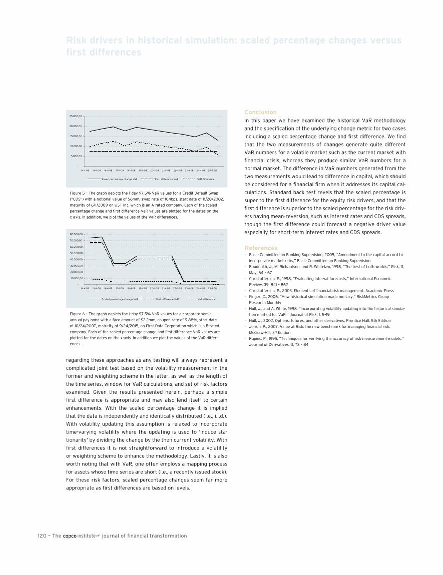
120 – The journal of financial transformation
risk drivers in historical simulation: scaled percentage changes versus first differences
regarding these approaches as any testing will always represent a
complicated joint test based on the volatility measurement in the
former and weighting scheme in the latter, as well as the length of
the time series, window for VaR calculations, and set of risk factors
examined. Given the results presented herein, perhaps a simple
first difference is appropriate and may also lend itself to certain
enhancements. With the scaled percentage change it is implied
that the data is independently and identically distributed (i.e., i.i.d.).
With volatility updating this assumption is relaxed to incorporate
time-varying volatility where the updating is used to ‘induce sta-
tionarity’ by dividing the change by the then current volatility. With
first differences it is not straightforward to introduce a volatility
or weighting scheme to enhance the methodology. Lastly, it is also
worth noting that with VaR, one often employs a mapping process
for assets whose time series are short (i.e., a recently issued stock).
For these risk factors, scaled percentage changes seem far more
appropriate as first differences are based on levels.
conclusionIn this paper we have examined the historical VaR methodology
and the specification of the underlying change metric for two cases
including a scaled percentage change and first difference. We find
that the two measurements of changes generate quite different
VaR numbers for a volatile market such as the current market with
financial crisis, whereas they produce similar VaR numbers for a
normal market. The difference in VaR numbers generated from the
two measurements would lead to difference in capital, which should
be considered for a financial firm when it addresses its capital cal-
culations. Standard back test revels that the scaled percentage is
super to the first difference for the equity risk drivers, and that the
first difference is superior to the scaled percentage for the risk driv-
ers having mean-reversion, such as interest rates and CDS spreads,
though the first difference could forecast a negative driver value
especially for short-term interest rates and CDS spreads.
references• Basle Committee on Banking Supervision, 2005, “Amendment to the capital accord to
incorporate market risks,” Basle Committee on Banking Supervision
• Boudoukh, J., M. Richardson, and R. Whitelaw, 1998, “The best of both worlds,” Risk, 11,
May, 64 – 67
• Christoffersen, P., 1998, “Evaluating interval forecasts,” International Economic
Review, 39, 841 – 862
• Christoffersen, P., 2003, Elements of financial risk management, Academic Press
• Finger, C., 2006, “How historical simulation made me lazy,” RiskMetrics Group
Research Monthly
• Hull, J., and A. White, 1998, “Incorporating volatility updating into the historical simula-
tion method for VaR,” Journal of Risk, 1, 5–19
• Hull, J., 2002, Options, futures, and other derivatives, Prentice Hall, 5th Edition
• Jorion, P., 2007, Value at Risk: the new benchmark for managing financial risk,
McGraw-Hill, 3rd Edition
• Kupiec, P., 1995, “Techniques for verifying the accuracy of risk measurement models,”
Journal of Derivatives, 3, 73 – 84
Figure 5 – The graph depicts the 1-day 97.5% VaR values for a Credit Default Swap
("CDS") with a notional value of $6mm, swap rate of 104bps, start date of 11/20/2002,
maturity of 6/1/2009 on UST Inc. which is an A-rated company. Each of the scaled
percentage change and first difference VaR values are plotted for the dates on the
x-axis. In addition, we plot the values of the VaR differences.
Figure 6 – The graph depicts the 1-day 97.5% VaR values for a corporate semi-
annual pay bond with a face amount of $2.2mm, coupon rate of 9.88%, start date
of 10/24/2007, maturity of 9/24/2015, on First Data Corporation which is a B-rated
company. Each of the scaled percentage change and first difference VaR values are
plotted for the dates on the x-axis. In addition we plot the values of the VaR differ-
ences.
-
5.000,00
10.000,00
15.000,00
20.000,00
25.000,00
Scaled percentage change VaR First difference VaR VaR difference
-
10.000,00
20.000,00
30.000,00
40.000,00
50.000,00
60.000,00
70.000,00
80.000,00
Scaled percentage change VaR First difference VaR VaR difference
-
5.000,00
10.000,00
15.000,00
20.000,00
25.000,00
Scaled percentage change VaR First difference VaR VaR difference
-
10.000,00
20.000,00
30.000,00
40.000,00
50.000,00
60.000,00
70.000,00
80.000,00
Scaled percentage change VaR First difference VaR VaR difference
14-4-08 15-4-08 16-4-08 17-4-08 18-4-08 19-4-08 20-4-08 21-4-08 22-4-08 23-4-08 24-4-08 25-4-08
14-4-08 15-4-08 16-4-08 17-4-08 18-4-08 19-4-08 20-4-08 21-4-08 22-4-08 23-4-08 24-4-08 25-4-08

121
risk drivers in historical simulation: scaled percentage changes versus first differences
Appendix
scaled Percentage change first Difference
risk factor # of E[failures] failures % of lruc lrind lrcc sig. failures % of lruc lrind lrcc sig. Var obs. obs. obs.
Panel A. Interest rates
6 month U.S.$ rate 3,782 37.82 46 1.2163% 1.6718 24.4183 26.0901 y,n,n 39 1.0312% 0.0368 11.8759 11.9127 y,n,n
2 year U.S.$ rate 3,782 37.82 57 1.5071% 8.5027 1.1448 9.6475 n,y,n 37 0.9783% 0.0181 0.7784 0.7965 y,y,y
5 year U.S.$ rate 3,782 37.82 48 1.2692% 2.5505 2.0556 4.6062 y,y,n 37 0.9783% 0.0181 0.7784 0.7965 y,y,y
10 year U.S.$ rate 3,782 37.82 40 1.0576% 0.1246 0.5833 0.7079 y,y,y 34 0.8990% 0.4034 0.6170 1.0205 y,y,y
6 month JPY rate 3,378 33.78 66 1.7451% 24.2832 9.7359 34.0191 n,n,n 32 0.9473% 0.0964 0.6123 0.7087 y,y,y
2 year JPY rate 3,378 33.78 48 1.4210% 5.3484 4.4827 9.8312 n,n,n 34 1.0065% 0.0014 3.9122 3.9136 y,n,y
5 year JPY rate 3,378 33.78 45 1.3321% 3.4091 1.2155 4.6246 n,y,n 29 0.8585% 0.7176 0.5024 1.2200 y,y,y
10 year JPY rate 3,378 33.78 49 1.4506% 6.0806 4.2824 10.3630 n,n,n 31 0.9177% 0.2376 1.1164 1.3541 y,y,y
Generic Corporate BBB 6 month U.S.$ rate 3,008 30.08 29 0.9641% 0.0396 1.1442 1.1838 y,y,y 24 0.7979% 1.3337 0.3862 1.7199 y,y,y
Generic Corporate BBB 2 year U.S.$ rate 3,008 30.08 35 1.1636% 0.7723 0.6313 1.4036 y,y,y 29 0.9641% 0.0396 0.5648 0.6045 y,y,y
Generic Corporate BBB 5 year U.S.$ rate 3,008 30.08 36 1.1968% 1.1072 3.1426 4.2497 y,n,y 33 1.0971% 0.2776 3.7277 4.0053 y,n,y
Generic Corporate BBB 10 year U.S.$ rate 3,008 30.08 36 1.1968% 1.1072 0.5637 1.6709 y,y,y 30 0.9973% 0.0002 1.0447 1.0449 y,y,y
Generic Corporate BB 6 month U.S.$ rate 3,008 30.08 27 0.8976% 0.3299 0.4893 0.8192 y,y,y 24 0.7979% 1.3337 0.3862 1.7199 y,y,y
Generic Corporate BB 2 year U.S.$ rate 3,008 30.08 30 0.9973% 0.0002 0.6046 0.6049 y,y,y 32 1.0638% 0.1213 0.6884 0.8097 y,y,y
Generic Corporate BB 5 year U.S.$ rate 3,008 30.08 34 1.1303% 0.4952 0.7777 1.2728 y,y,y 25 0.8311% 0.9194 0.4192 1.3386 y,y,y
Generic Corporate BB 10 year U.S.$ rate 3,008 30.08 35 1.1636% 0.7723 0.8244 1.5966 y,y,y 29 0.9641% 0.0396 0.5648 0.6045 y,y,y
Panel B. foreign Exchange rates
U.S.$/JPY FX rate 3,791 37.91 40 1.0551% 0.1143 0.5861 0.7004 y,y,y 33 0.8705% 0.6717 1.1003 1.7720 y,y,y
U.S.$/GBP FX rate 3,791 37.91 27 0.7122% 3.5253 1.7309 5.2562 n,y,n 31 0.8177% 1.3566 0.5113 1.8679 y,y,y
U.S.$/EUR FX rate 2,227 22.27 21 0.9430% 0.0746 0.4000 0.4746 y,y,y 19 0.8532% 0.5104 0.3271 0.8375 y,y,y
scaled Percentage change first Difference
risk factor # of E[failures] failures % of lruc lrind lrcc sig. failures % of lruc lrind lrcc sig. Var obs. obs. obs.
Panel A — Equities
S&P 500 index 3,652 36.52 42 1.1501% 0.7923 2.7614 3.5537 y,y,y 42 1.1501% 0.7923 2.7614 3.5537 y,n,y
IBM Corporation 3,652 36.52 37 1.0131% 0.0063 0.7333 0.7396 y,y,y 40 1.0953% 0.3249 3.0747 3.3996 y,n,y
Amazon.com Inc. 2,548 25.48 30 1.1774% 0.7663 0.7152 1.4815 y,y,y 34 1.3344% 2.6045 2.9859 5.5904 y,n,n
VIX index 3,652 36.52 54 1.4786% 7.3660 0.0485 7.4145 n,y,n 41 1.1227% 0.5339 6.4930 7.0270 y,n,n
Panel B — commodities
1 month crude oil 3,630 36.30 37 1.0193% 0.0135 0.7256 0.7392 y,y,y 45 1.2397% 1.9571 2.3173 4.2744 y,y,y
1 month natural gas 3,630 36.30 36 0.9917% 0.0025 0.7214 0.7239 y,y,y 33 0.9091% 0.3126 8.8747 9.1873 y,n,n
Panel c — Generic credit default swap spreads
Generic corporate BBB 6 month CDS 1,182 11.82 55 4.6531% 84.3827 0.0787 84.4614 n,y,n 12 1.0152% 0.0028 2.5863 2.5890 y,y,y
Generic corporate BBB 3 year CDS 1,182 11.82 16 1.3536% 1.3444 0.4395 1.7839 y,y,y 17 1.4382% 2.0193 5.2768 7.2960 y,n,n
Generic corporate BBB 5 year CDS 1,182 11.82 12 1.0152% 0.0028 0.2464 0.2491 y,y,y 14 1.1844% 0.3835 2.0272 2.4106 y,y,y
Generic corporate BBB 10 year CDS 1,182 11.82 14 1.1844% 0.3835 0.3359 0.7194 y,y,y 17 1.4382% 2.0193 0.4966 2.5158 y,y,y
Generic corporate BB 6 month CDS 1,182 11.82 68 5.7530% 128.3426 0.3141 128.6567 n,y,n 15 1.2690% 0.7964 1.7878 2.5842 y,y,y
Generic corporate BB 3 year CDS 1,182 11.82 13 1.0998% 0.1153 2.2921 2.4074 y,y,y 12 1.0152% 0.0028 0.2464 0.2491 y,y,y
Generic corporate BB 5 year CDS 1,182 11.82 13 1.0998% 0.1153 0.2894 0.4046 y,y,y 8 0.6768% 1.4068 0.1091 1.5160 y,y,y
Generic corporate BB 10 year CDS 1,182 11.82 18 1.5228% 2.8135 0.5572 3.3707 n,y,y 14 1.1844% 0.3835 2.0272 2.4106 y,y,y
Figure A1 – For fixed income (i.e. interest rates) and foreign exchange spot rates the table provides a description of the relevant risk factors in each panel, the total number of VaR
observations, expected number of failures (i.e., product of VaR observations and alpha), and results for each of the scaled percentage change and first difference. For each change mea-
sure the table includes the total failures, percent of observations, LRuc, LRind, and LRcc statistics. The failure results are based on a 1% alpha or 99% P-value. If the test statistic values
are less than the associated Chi-square test statistic values then one would fail to reject the null hypothesis and the VaR model is deemed statistically sound. The Chi-square test statis-
tics for a 10% probability value for one and two degrees of freedom are 2.7055 and 4.6052 respectively. (y indicates that we fail to reject the null hypothesis, n indicates that we reject
the null hypothesis. The Sig. column indicates whether or not the test statistic is significant for each of the three values respectively.)
Figure A2 – For equities, commodities, and generic credit default swap spread the table provides a description of the relevant risk factors in each panel, the total number of VaR obser-
vations, expected number of failures (i.e., product of VaR observations and alpha), and results for each of the scaled percentage change and first difference. For each change measure
the table includes the total failures, percent of observations, LRuc, LRind, and LRcc statistics. The failure results are based on a 1% alpha or 99% P-value. If the test statistic values are
less than the associated Chi-square test statistic values then one would fail to reject the null hypothesis and the VaR model is deemed statistically sound. The Chi-square test statistics
for a 10% probability value for one and two degrees of freedom are 2.7055 and 4.6052 respectively. (y indicates that we fail to reject the null hypothesis, n indicates that we reject the
null hypothesis, the Sig. column indicates whether or not the test statistic is significant for each of the three values respectively.)


123
AbstractWe study the impact that hedge fund family membership has on
performance and market share. Hedge funds from small fund
families outperform those from large families by a statistically
significant 4.4% per year on a risk-adjusted basis. We investigate
the possible causes for this outperformance and find that regard-
less of family size, fund families that focus their efforts on their
core competencies have ‘core competency’ funds with superior
performance, while the same family’s non-core competency funds
underperform. We next examine the determinants of hedge fund
family market share. A family’s market share is positively related
to the number and diversity of funds offered, and is also positively
related to past fund performance. Finally, we examine the determi-
nants of fund family market share at the fund style/strategy level.
Families that focus on their core competencies attract positive and
significant market share to these core-competency funds. Hence,
by starting new funds only in their family’s core competencies, fund
managers can enjoy increased market share while their investors
enjoy good performance.
The impact of hedge fund family membership on performance and market share
Part 2
nicole M. BoysonAssistant Professor of Finance,
Northeastern University

124 – The journal of financial transformation
We study the impact that family membership has on hedge funds.
Based on data provided by Tremont Shareholder Advisory Services
(TASS), in 1994 about 70% of all hedge funds were ‘stand-alone’
funds where the manager/management company oversaw only
one hedge fund. This ratio has steadily declined, reaching a value
of just under 50% in 2007. Furthermore, the number of hedge fund
families (defined as hedge fund management companies) with 10
or more member funds has grown from 10 families to 228 families
over the same time period, a 2,180% increase. Clearly, managers
perceive some benefit from expanding their offerings and starting
additional hedge funds. In this paper, we investigate the possible
motivation for families to start new funds, as well as the costs and
benefits accruing to fund investors.
Although there are a number of recent studies regarding mutual
fund families, ours is the first to examine hedge fund families.
Studies of mutual funds find that mutual fund families: 1) favor cer-
tain funds within their families over others, and allocate their best
resources to these funds, 2) start new funds in different strategies
to attract new investors and to provide more choices to existing
investors, 3) start new funds in strategies in which they already
have good performers, 4) are often successful in attracting new
cash flows, even if many of their existing funds are poor performers,
and 5) tend to attract assets to all their funds (even the poor per-
formers) if they have at least one top-performing fund [Guedj and
Papastaikoudi (2005), Gaspar et al. (2006), Khorana and Servaes
(1999), Zhao (2005), Massa (2003), Berzins (2005), Siggelkow
(2003), Nanda et al. (2004)]. In addition, families that focus on their
core competencies tend to outperform families that do not. Finally,
Khorana and Servaes (2007) argue that mutual fund managers face
a conflict of interest between attracting market share and maximiz-
ing the performance of their funds, and find some evidence that this
conflict drives managerial behavior. However, they also find that
mutual fund investors are fairly sophisticated and do consider fund
performance when making investment decisions.
Drawing from this literature, we focus on two research questions
for our study of hedge funds. First, is hedge fund family size and
focus related to hedge fund performance? We show that although
hedge funds from single-fund families generally outperform hedge
funds from larger families, families that focus on their core com-
petencies outperform families that do not, independent of family
size and the number of funds offered. By contrast, funds not within
a fund family’s core competency tend to underperform. These
results are largely consistent with Siggelkow (2003). Second, why
do hedge fund families start new funds? We are mainly interested
in potential conflicts of interest between hedge fund managers and
investors. These conflicts might occur because managers wish to
increase their fund and family market share (maximizing their fee
income) while investors simply want the best performance pos-
sible. We perform two analyses, one at the fund family level and
one at the fund style level (within a fund family). At the family level,
market share increases as the number of hedge funds in a family
increase. Furthermore, families with strong past performance enjoy
increased market share. At fund style level, families that concen-
trate their assets in fewer style categories enjoy higher market
share, and having past expertise in these style categories also
improves their market share.
Our interpretation of these findings is that the desire of fund man-
agers to expand their market share is not necessarily at odds with
the desire of investors to achieve good performance. For fund fami-
lies that expand their offerings into style categories in which they
already have proficiency, they can enjoy both strong market share
and good fund performance. However, for fund families that expand
their offerings into areas in which they have not demonstrated
expertise, the results are beneficial to families but detrimental to
investors: market share increases as fund performance declines.
The impact of hedge fund family membership on performance and market share
Year number of Mean funds Maximum funds Mean styles Maximum styles number of number of number of Top style families per family per family per family per family one-fund families families with 10 funds or more funds
1994 703 1.65 14 1.15 4 497 10 1,160 Managed futures
1995 873 1.72 17 1.17 5 593 13 1,503 Long/short equity
1996 1,074 1.77 18 1.18 5 708 16 1,905 Long/short equity
1997 1,293 1.82 18 1.18 5 828 20 2,348 Long/short equity
1998 1,516 1.85 20 1.18 5 964 22 2,805 Long/short equity
1999 1,752 1.92 23 1.2 6 1,079 30 3,362 Long/short equity
2000 2,023 1.97 25 1.2 6 1,226 34 3,977 Long/short equity
2001 2,292 2.11 25 1.21 8 1,347 52 4,838 Long/short equity
2002 2,595 2.25 32 1.23 8 1,479 71 5,837 Long/short equity
2003 2,889 2.43 39 1.25 8 1,574 100 7,034 Long/short equity
2004 3,189 2.65 61 1.27 9 1,675 136 8,466 Long/short equity
2005 3,495 2.82 83 1.3 9 1,793 169 9,870 Fund of funds
2006 3,729 2.96 92 1.32 9 1,865 204 11,044 Fund of funds
2007 3,897 3.10 100 1.33 9 1,933 228 12,090 Fund of funds
Figure 1 – Summary statistics for hedge fund families

125
DataData is provided by Credit Suisse/Tremont Advisory Shareholder
Services (TASS) for the time period 1994-2007. This database
includes data on returns, fees, size, notice and redemption periods,
management company, and investment styles of hedge funds. We
denote funds with the same management company as belonging to
the same ‘fund family’. There are eleven investment styles in the
database: convertible arbitrage, dedicated short sellers, emerging
markets, equity market neutral, event driven, fixed income arbi-
trage, funds of funds, global macro, long/short equity, managed
futures, and multi-strategy1. Hedge fund databases suffer from
several biases including survivorship bias and instant history or
backfilling bias [Ackermann et al. (1999), Fung and Hsieh (2000),
Liang (1999), Brown et al. (2001)]. We control for survivorship bias
by including defunct funds until they disappear from the database
and mitigate backfilling bias by excluding the fund’s ‘incubation
period’ from the time-series of returns2.
Figure 1 presents summary statistics regarding the number of
families, number of funds, and investment styles. Some interesting
trends in the data are notable. First, the number of fund families
and the number of funds has grown dramatically, from 703 (1,160)
families (funds) in 1994 to 3,897 (12,090) families (funds) in 2007.
Second, the average number of funds per family has grown from
1.7 to 3.1 over the same time. Third, the proportion of fund families
with only one fund (stand-alone funds) has decreased from 70%
in 1994 to 50% in 2007. Fourth, the number of families with 10 or
more funds has increased, from 10 families in 1994 to 228 families
in 2007. Finally, the most popular fund style was long/short equity
for most of the sample period, but was overtaken by funds of funds
beginning in 2005.
Impact of family membership and other characteristics on fund performanceIn this section, we test whether family size is related to perfor-
mance. We perform the following analysis for fund i in family k in
category j at time t: perfmeasureikjt = constant + β1number of funds
in familyk,t + β2annual standard deviationit + β3annual standard
deviationi,t-1 + β4log fund sizei,t-1 + β5fund agei,t-1 + β6fund flowi,t-1
+ β7management feei,t-1 + β8incentive feei,t-1 + β9log minimum
investmenti,t-1 + β10high water mark dummyi,t-1 + β11uses leverage
dummyi,t-1 + β12personal capital invested dummyi,t-1 + β13open to
new investment dummyi,t-1 + β14open to non-accredited investors
dummyi,t-1 + β15lockup period in monthsi,t-1 (1)
The regression also includes 10 style category dummies (the global
macro-style category is excluded), and year dummy variables (1994
is excluded). We use an OLS regression, pooling the time-series and
the cross-section. As noted by Brav (2000) and Petersen (2008),
cross-sectional correlation across fund residuals in the same year
can lead to improperly stated standard errors. To correct for this
problem, as well as any unobserved autocorrelation, we use White
(1980) standard errors (to account for autocorrelation) adjusted to
account for cross-sectional correlation within two separate clus-
ters; clusters include both fund and time3.
We use three separate performance measures. The first is the
intercept (alpha) from 36–month regressions using the Carhart
(1997) four-factor model [see Carhart (1997) for detail on the four
factors]. Data for all these factors comes from the website of
Kenneth French. The second measure uses the factors of Fung and
Hsieh (2004), designed specifically for hedge funds. Their original
model includes seven factors, but we include an additional factor,
the MSCI Emerging Markets Index return, as suggested by David
Hsieh’s website [See Fung and Hsieh (2004) for detail on the seven
factors]. Data for these factors is from the website of David Hsieh.
Finally, the third return measure is the annual return of the hedge
fund, less the risk-free rate.
A few of the independent variables require explanation. The first is
fund flow, which is the annual net inflows/outflows to/from a fund
scaled by prior year fund size. The second is fund age, calculated
using the fund’s start date. Additionally included are indicator vari-
ables for high water mark, uses leverage, invests personal capital,
fund is open to new investment, and fund is open to non-accredited
investors. In interpreting the regression results, a negative and
significant coefficient on the lagged number of funds per family (β1)
The impact of hedge fund family membership on performance and market share
1 See www.hedgeindex.com for a description of investment styles.
2 To mitigate the incubation bias, we use data from the ‘performance start date’ rather
than the ‘inception date’ from the TASS database.
3 This correction is also known as the Rogers (1993) correction, and controls for auto-
correlation over the entire time-series of each fund’s observations. This adjustment
may be contrasted with the Newey-West (1987) correction for autocorrelation, which
can be specified up to a particular lag length. As Petersen (2008) notes, the Rogers
(1993) correction produces unbiased estimates, while the Newey-West (1987) correc-
tion will lead to biased estimates (although the longer the lag length, the smaller the
bias). The approach also controls for cross-correlation, to address the issue noted by
Brav (2000). Petersen (2008) describes the approach that we follow in this paper,
where we cluster both fund and time to adjust standard errors for both types of
potential auto- and cross-correlation. We thank Mitchell Petersen for providing us the
STATA code for this analysis.
Annual return four factor Eight factor net of alpha alpha Dependent variable: risk-free rate (annualized) (annualized)
Constant -0.008 -0.202*** -0.150***
(-0.11) (-6.14) (-3.37)
Number of funds per family -0.0003*** -0.001*** -0.0005***
(-2.40) (-3.72) (-3.81)
Lagged log (size) 0.104 0.173* 0.082
(0.65) (1.69) (0.96)
Lagged age in years -0.003 0.005*** 0.006***
(-0.93) (4.15) (5.03)
Lagged flow 0.000 0.003*** 0.003***
(-0.23) (4.23) (4.34)
Number of Observations 16,660 16,660 16,660
Adjusted R2 13.6 11.2 13.4
Fund performance is regressed on number of funds per family and a number of con-
trol variables, as defined in Equation (1).
Regressions are performed using annual data at the fund level in a pooled time-
series, cross-sectional setting. For brevity, not all coefficients are reported.
t-statistics using White standard errors adjusted for correlation within two clusters
(also known as Rogers standard errors with clustering at the fund level and at time
level) are shown below the coefficients in parentheses. The regressions also include
time trend variables and indicator variables for fund style (not reported for brevity).
Coefficients marked with ***, **, and * are statistically significant at the 1%, 5%, and
10% levels, respectively.
Figure 2 – Multivariate regressions of performance on number of funds in family

126 – The journal of financial transformation
implies families with more funds underperform. The results are pre-
sented in Figure 2. For all three performance measures, the number
of funds in a family is negatively associated with fund performance
at the 1% significance level. Also, fund size, management fees,
minimum investment, and lockup period are positively related to
performance, while fund age is negatively related to performance
[Agarwal and Naik (1998), Liang (1999), Brown et al. (2001), Amenc
et al. (2003), Getmansky (2005)].
We further investigate the factors driving this result by examining
whether it can be attributed to product focus; a hedge fund fam-
ily’s degree of specialization in a style category. There are two
competing hypotheses regarding the impact of product focus on
firm profitability. First, by specializing in a style category, the fund
family can achieve good performance. Second, fund families that
are too specialized will miss out on opportunities to improve profit-
ability through expansion into other styles. Prior literature regard-
ing corporate acquisitions and divestitures finds that product focus
is positively related to performance [Morck et al. (1990), Comment
and Jarrell (1995), John and Ofek (1995)].
The idea of focus (at the fund family level) can be delineated into
two concepts. Firstly is relatedness, implying that funds in the
family’s core competency (the fund style in which the family has
significant expertise) should outperform non-core compentency
funds [per Siggelkow (2003), the family’s fringe funds]. The second
concept is narrowness, implying that fund families active in fewer
styles will have lower monitoring costs, so even fringe funds from
narrow families will outperform funds from other families.
To test focus, relatedness, and narrowness, we perform two sets of
regressions. The first regressions test the concept of focus, using
the following variable calculated at the fund family level and analo-
gous to the Herfindahl index:
focuskt = = (2),
where the sum is taken over all categories j in family k at time t.
The second regressions test relatedness and narrowness.
Relatedness is calculated at the fund level, as:
relatedit = (3)
This variable will therefore be higher for funds in the family’s core
competency and lower for fringe funds. For narrowness we use
the variable categorieskt, a count of the total number of style cat-
egories within a fund family k at time t, which is measured at the
family level. Hence, it actually measures broadness (or inverse of
narrowness).
The first regression performs the analysis for fund i in family k in cat-
egory j at time t: perfmeasureikjt = constant + β1focuskt + β2annual
standard deviationit + β3annual standard deviationi,t-1 + β4log fund
sizei,t-1 + β5fund agei,t-1 + β6fund flowi,t-1 + β7management feei,t-1 +
β8incentive feei,t-1 + β9log minimum investmenti,t-1 + β10high water
mark dummyi,t-1 + β11uses leverage dummyi,t-1 + β12personal capi-
tal invested dummyi,t-1 + β13open to new investment dummyi,t-1 +
β14open to non-accredited investors dummyi,t-1 + β15lockup period in
monthsi,t-1 + β16log of family assets(size)k,t-1 + β17log of family assets
in same style (size)kj,t-1 + β18number of funds in own family in same
stylekj,t + β19total number of funds across families in same stylej,t +
β20fund market share relative to its stylekj,t-1 (4).
All control variables were described above, except ‘log of family
assets (size),’ the log of family assets under management, ‘log of
family assets in same style (size),’ the log of family assets under
management in the same style as fund i, ‘number of funds in own
family in same style,’ ‘total number of funds across families in same
style,’ and ‘fund market share relative to its style,’ the total assets
in fund i scaled by the total assets in fund i’s style category (across
all funds in all families). These additional variables are included
since funds in large families could have better economies of scale
or monitoring ability, and to control for general competitive effects.
Time trend and style category dummy variables are also included.
The impact of hedge fund family membership on performance and market share
Includes focus Includes relatedness and categories
four factor Eight factor four factor Eight factor alpha alpha alpha alpha Dependent Variable: (annualized) (annualized) (annualized) (annualized)
Constant -0.203*** -0.148*** -0.218*** -0.160***
(-5.51) (-3.06) (-5.97) (-3.26)
Focus measure 0.010 0.004
(1.14) (0.51)
Relatedness measure 0.025*** 0.016***
(2.60) (2.54)
Categories measure -0.002 -0.001
(-1.46) (-0.94)
Lagged log (size) 0.008*** 0.008*** 0.008*** 0.008***
(6.40) (4.74) (5.99) (4.55)
Lagged age in years -0.003*** -0.003*** -0.003*** -0.003***
(-4.18) (-4.57) (-4.27) (-4.63)
Lagged flow 0.003*** -0.003*** -0.003*** -0.003***
(4.23) (4.32) (4.22) (4.31)
Number of observations 16,660 16,660 16,660 16,660
Adjusted R2 11.7 13.4 11.9 13.4
Fund performance is regressed on focus, relatedness, and categories and a number
of control variables, as defined in Equation (4). Regressions are performed using
annual data at the fund level in a pooled time-series, cross-sectional setting. For
brevity, not all coefficients are reported. t-statistics using White standard errors
adjusted for correlation within two clusters (also known as Rogers standard errors
with clustering at the fund level and at time level) are shown below the coefficients in
parentheses. The regressions also include time trend variables and indicator variables
for fund style (not reported for brevity). Coefficients marked with ***, **, and * are
statistically significant at the 1%, 5%, and 10% levels, respectively.
Figure 3 – Focus, relatedness, and categories regressions
Assets of family k in category j at time t
Total assets of family k at time t
Σj
Assets of family k in category j at time t
Total assets of family k at time t

1274 As a robustness test, we also perform the analysis excluding families with only one
fund. We perform this test because, by definition, families with only one fund will have
maximum values for related and focus and a minimum value of categories, which could
be driving our results, since families with only one fund make up the majority of the
sample in many years. Dropping families with only 1 fund produces virtually identical
results. We also perform these same robustness tests dropping families with 2 or 3
funds, and again, find very similar results to those reported in the paper.
5 Of course, this does not imply that managers do not also care about performance,
especially since their incentive fees are tied to performance and managers often
invest large percentage of their personal capital in their funds. However, the desire to
obtain market share is also relevant.
The impact of hedge fund family membership on performance and market share
The second set of regressions includes these control variables, but
substitutes for focus the variables related and categories. Figure
3 presents results. In contrast with Siggelkow (2003), there is no
significant evidence that focus is related to fund performance.
However, we find strong evidence that focus-related factors are
important in the second regression specification. The positive
and significant coefficient on related indicates that for families
specializing in few style categories the funds in those categories
outperform fringe funds. This result is consistent with Siggelkow’s
(2003) study of mutual funds. The coefficient on the categories
variable, a measure of broadness of offerings within a fund fam-
ily, is negative but not statistically significant. The negative sign
implies that hedge funds from families investing in many style
categories do not outperform those from families that invest in
fewer style categories4.
Next, we interpret these results. At the family level, we cannot
make broad statements about the performance of hedge funds
in families that focus versus families that do not. However, at the
individual fund level, we have found an important relationship.
Individual funds in a family’s core competency outperform funds
not in the family’s core competency. Hence, an investor need not
avoid all hedge funds from large families, but rather should only
select funds within the family’s core competency. Furthermore, an
investor would do well to avoid families that diversify across too
many different categories, since although the categories variable
is not significant in Figure 3, a separate regression analysis (not
reported) including the categories variable but not the related vari-
able has a significantly negative coefficient on categories.
Market share and hedge fund familiesThis section focuses on hedge fund market share, in an approach
similar to Khorana and Servaes (2007). Hedge fund managers
receive both management fees based on assets and incentive fees
based on profits. Both fees provide incentives for managers to grow
their funds. Hence, hedge fund managers and investors could have
conflicting goals if managers focus more on market share than on
performance5.
We perform two market share analyses, at the family level and at
the style level. For families with only one style, these data will be
identical, but for families with more than one style, these data will
differ. The regression specification at the family level for family
k at time t is as follows: logmktsharekt = constant + β1focusk(t-1)
+ β2categoriesk(t-1) + β3total number of funds in familyk(t-1) +
β4dummy for top 5% performer in familyk(t-1) + β5number of new
funds in familyk(t-1) + β6family performancek(t-1) + β7average family
agek(t-1) + β8average family incentive feek(t-1) + β9average family
management feek(t-1) + β10high water mark dummyk(t-1) + β11uses
leverage dummyk(t-1) + β12personal capital invested dummyk(t-1) +
β13open to new investment dummyk(t-1) + β14open to non-accred-
ited investors dummyk(t-1) + β15average family lockup period in
monthsk(t-1) (5)
This regression also includes time trend variables. The other
controls are self-explanatory or are as in Figures 2 and 3, except
here they are averaged across families, as these regressions are
performed at the family level. The dependent variable, logmarket-
share, is the log of the market share of the family (total assets in
specification 1 – specification 2 – specification 3 – specification 4 – Performance measure Performance measure Performance measure Performance measure Dependent variable: is equally-weighted is equally-weighted is equally-weighted is equally-weighted log of family market share four factor alpha four factor alpha eight factor alpha eight factor alpha
Constant -8.729*** -8.745*** -8.672*** -8.711***
(-16.94) (-16.94) (-16.58) (-16.76)
Lagged focus measure -0.962*** -0.957*** -0.939** -0.960***
(-2.41) (-2.40) (-2.32) (-2.39)
Lagged categories measure 0.166* 0.159* 0.154* 0.156*
(1.85) (1.76) (1.71) (1.74)
Lagged number of funds in family 0.041*** 0.043*** 0.042*** 0.042***
(2.53) (2.64) (2.64) (2.65)
Lagged dummy: top 5% fund in family -0.109 -0.107 0.071 -0.048
(-1.52) (-1.51) (0.98) (-0.74)
Lagged number of new funds by family 0.152*** 0.150*** 0.142*** 0.148***
(3.31) (3.22) (3.06) (3.20)
Family lagged risk-adjusted return 1.455*** 1.251*** 0.093** 0.748***
(5.25) (2.91) (1.95) (2.43)
Number of observations 3,598 3,598 3,598 3,598
Adjusted R2 33.2 33.0 32.4 32.7
Log of fund family market share is regressed on a number of variables, as described in Equation (5). OLS regressions are performed using annual data at the fund family level in a
pooled time-series, cross-sectional setting. For brevity, not all coefficients are reported. t-statistics using White standard errors adjusted for correlation within two clusters (also known
as Rogers standard errors with clustering at the family level and at time level) are shown below the coefficients in parentheses. The regressions also include time trend variables (not
reported for brevity). Coefficients marked with ***, **, and * are statistically significant at the 1%, 5%, and 10% levels, respectively.
Figure 4 – Market share regressions at the fund family level

128 – The journal of financial transformation
The impact of hedge fund family membership on performance and market share
the family at time t ÷ total assets across all families at time t). An
additional independent variable: dummy for top 5% performer in
family is introduced. This is a dummy variable set to 1 if the fund
family has at least 1 fund in the top 5% of all funds (based on its
four or eight factor alpha) in year t.
The regression specifications are identical except for the indepen-
dent variable measuring family performance. Specification 1 (2) uses
a four-factor alpha assuming an equally-weighted (value-weighted)
portfolio of funds in each family. Specification 3 (4) uses an eight-
factor alpha assuming an equally-weighted (value-weighted) port-
folio of funds in each family. In Figure 4, the coefficient on focus
is significantly negative in all specifications, implying that families
have incentives to diversify across fund styles to increase market
share. Also, the coefficient on categories is significantly positive
in all four specifications, implying that offering more unique fund
styles improves market share. Finally, the prior performance of the
family is also significantly positively related to market share. While
these results suggest that families face competing incentives (since
having more funds in a family increases market share per Figure
4, but reduces performance per Figure 2), they are not conclusive
since regressions are performed at the family level, and not at
the fund or style category level. Furthermore, since market share
increases with family performance, managers have incentives to
perform well, consistent with the objectives of their investors. We
also reperform the regressions excluding one-fund families. The
findings are consistent with Figure 4.
Figure 5 performs an analysis of market share at the fund style
level within each family. Here, the dependent variable’s unit of
measurement is the log of market share of a fund style category
within a fund family (or total assets in style category j within fund
family k at time t ÷ total assets in style category j across all fund
families at time t). With this specification, we can more directly
test the alignment of incentives between families and investors.
We are particularly interested in whether market share by style
category within a fund family is higher for families focusing on
their core competencies. The regression specification is as fol-
lows: logmktsharekjt = constant + β1relatedkj(t-1) + β2total number
of funds in familyk(t-1) + β3total number of funds in category j in
familykj(t-1) + β4number of new funds in familyk(t-1) + β5number of
new funds in category j in familykj(t-1) + β6dummy for top 5% per-
former in familyk(t-1) + β7dummy for top 5% performer in category
j in familyk(t-1) + β8family performancek(t-1) + β9performance of cat-
egory j in familyk(t-1) + β10average family agek(t-1) + β11average age
of category j in familykj(t-1) + β12average family incentive feek(t-1) +
β13average incentive fee of category j in familykj(t-1) + β14average
family management feek(t-1) + β15average management fee of cat-
egory j in familykj(t-1) + β16high water mark dummy at the family
levelk(t-1) + β17high water mark dummy of category in familykj(t-1) +
β18uses leverage dummy at the family levelk(t-1) + β19uses leverage
dummy of category j in familykj(t-1) + β20personal capital invested
dummy at the family levelk(t-1) + β20personal capital invested
dummy of category j in familykj(t-1) + β21open to new investment
dummy at the family levelk(t-1) + β22open to new investment dummy
of category j in familykj(t-1) + β23open to non-accredited investors
specification 1 – specification 2 – specification 3 – specification 4 – Dependent variable: Performance measure Performance measure Performance measure Performance measure log of family market share is equally-weighted is equally-weighted is equally-weighted is equally-weighted by fund style category four factor alpha four factor alpha eight factor alpha eight factor alpha
Constant -6.941*** -6.942*** -6.980*** -6.973***
(-27.50) (-27.12) (-27.81) (-27.51)
Relatedness 0.299** 0.328** 0.297** 0.308**
(2.11) (2.29) (2.09) (2.12)
Lagged number of funds in family 0.038*** 0.037*** 0.037*** 0.038***
(3.17) (3.16) (3.12) (3.13)
Lagged number of funds in family by style category 0.104*** 0.102*** 0.109*** 0.107***
(3.98) (4.01) (4.29) (4.24)
Lagged number of new funds by family -0.014 -0.014 -0.013 -0.011
(-0.33) (-0.32) (-0.32) (-0.25)
Lagged number of new funds by family by style category 0.050 0.047 0.054 0.048
(0.95) (0.91) (1.04) (0.94)
Lagged top 5% fund in family dummy 0.926 0.967 0.581* 0.563*
(1.48) (1.59) (1.69) (1.71)
Lagged top 5% fund in family in style category dummy -0.992 -0.845 -0.727** -0.653*
(-1.60) (-1.43) (-2.03) (-1.92)
Adjusted R2 11.8 11.3 12.0 11.8
Log of fund family market share in each fund style category is regressed on a number of variables per Equation (5). OLS regressions are performed using annual data at the fund
style category within fund family level in a pooled time-series, cross-sectional setting. For brevity, not all coefficients are reported. t-statistics using White standard errors adjusted
for correlation within two clusters (also known as Rogers standard errors with clustering at the family level and at time level) are shown below the coefficients in parentheses. The
regressions also include time trend variables (not reported for brevity). Coefficients marked with ***, **, and * are statistically significant at the 1%, 5%, and 10% levels, respectively.
Figure 5 – Market share regressions at the fund style category within fund family level

1296 As with prior results, we reperform our tests excluding one-fund families and find
consistent results.
dummy at the family levelk(t-1) + β24open to non-accredited inves-
tors dummy of category j in familykj(t-1) + β25average family lockup
period in months at the family levelk(t-1) + β26average family lockup
period in months of category j in familykj(t-1) (6)
This regression includes time trend variables. The control variables
are measured at both the family level and the style category level
(within each fund family). In Figure 5, the coefficient on related is
significantly positive in all specifications, indicating that a family’s
market share is higher for style category(ies) within a family in the
manager’s core competency. Earlier Figure 3 results indicate that
these same core competency style categories have the best-per-
forming funds. Since both market share and performance increase
when managers focus on their core competencies, both manage-
rial and investor incentives can be achieved. Figure 5 also finds a
significant positive relationship between market share in a style
category and the number of funds in that category, also implying
that focusing on core competency funds increases market share.
Finally, the more experience a manager has in a particular category,
the more assets the manager attracts to that category6. Our results
are generally consistent with Khorana and Servaes (2007).
conclusionWe examine the relationship between hedge fund family member-
ship, performance, and market share. Unconditionally, families
with more funds underperform families with less funds. However,
regardless of size, families that focus on their core competencies
have good ‘core competency’ funds but poor ‘fringe’ funds (funds
outside of their core competencies). In other words, managers that
do not venture outside their skill sets outperform.
We also investigate the determinants of family market share.
Families with more diversity in their fund offerings have higher
market share. Families with good past performance also have
higher market share. Hence, fund managers must strike a balance
between improving market share and maintaining good perfor-
mance. One way that managers can achieve this goal is to focus
on their core competencies, since we show that for these funds,
both performance and market share is strong. Hence, managers
would do well to stick to their core competencies when opening
new funds.
Our results suggest the following. First, hedge fund investors should
not unconditionally avoid multi-fund families. Rather, they should
select funds from families in which the majority of the family’s funds
are core competency funds. Second, regardless of family size, hedge
fund investors should avoid funds outside the family’s core compe-
tencies. Finally, hedge fund managers should grow their families by
focusing on new funds within their core competencies, since these
funds attract the largest market share and are the best performers.
references• Ackermann, C., R. McEnally, and D. Ravenscraft, 1999, “The performance of hedge
funds: risk, return, and incentives,” Journal of Finance, 54, 833-873
• Agarwal, V. and N. Y. Naik, 1999, “On taking the alternative route: risks, rewards, style,
and performance persistence of hedge funds,” Journal of Alternative Investments, 2:4,
6-23
• Amenc, N., S. Curtis, and L. Martellini, 2003, “The alpha and omega of hedge fund per-
formance measurement,” Edhec Risk and Research Asset Management Centre
• Berzins, J., 2005, “Do families matter in institutional money management industry?
The case of new portfolio openings,” Norwegian School of Management working paper
• Brav, A., 2000, “Inference in long-horizon event studies: a Bayesian approach with
application to initial public offerings,” Journal of Finance, 55:5, 1979-2016
• Brown, S., W. Goetzmann, and J. Park, 2001, “Conditions for survival: changing risk and
the performance of hedge fund managers and CTAs,” Journal of Finance, 56:5, 1869-
1886
• Carhart, M., 1997, “On persistence in mutual fund performance,” Journal of Finance,
52:1, 57-82
• Comment, R. and G. A. Jarrell, 1995, “Corporate focus and stock returns,” Journal of
Financial Economics, 37, 67-87
• Fama, E. and K. French, 1992, “The cross-section of expected stock returns,” Journal of
Finance, 47:2, 427-465
• Fama, E., and K. French, 1993, “Common risk factors in the returns on bonds and
stocks,” Journal of Financial Economics, 33:1, 3-53
• Fung, W., and D. A. Hsieh, 2000, “Performance characteristics of hedge funds and com-
modity funds: natural versus spurious biases,” Journal of Financial and Quantitative
Analysis, 35, 291-307
• Fung, W., and D. A. Hsieh, 2001, “The risk in hedge fund strategies: theory and evidence
from trend followers,” Review of Financial Studies, 14, 313-341
• Fung, W., and D. A. Hsieh, 2004, “Hedge fund benchmarks: a risk-based approach,”
Financial Analysts Journal, 60, 65-81
• Gaspar, J., M. Massa, and P. Matos, 2006, ”Favoritism in mutual fund families?
Evidence on strategic cross-fund subsidization,” Journal of Finance, 61, 73-104
• Getmansky, M., 2005, “The life cycle of hedge funds: fund flows, size, and perfor-
mance,” Working paper, University of Massachusetts-Amherst
• Guedj, I., and J. Papastaikoudi, 2005, “Can mutual fund families affect the performance
of their funds?” University of Texas at Austin working paper
• Jegadeesh, N., and S. Titman, 1993, “Returns to buying winners and selling losers:
implications for stock market efficiency,” The Journal of Finance, 48:1, 93-130
• John K., and E. Ofek, 1995, “Asset sales and increase in focus,” Journal of Financial
Economics, 37, 105-126
• Khorana, A., and H. Servaes, 1999, “The determinants of mutual fund starts,” Review of
Financial Studies, 12:5, 1043-1074
• Khorana, A., and H. Servaes, 2007, “Competition and conflicts of interest in the U.S.
mutual fund industry,” London Business School working paper
• Liang, B., 1999, “On the performance of hedge funds,” Financial Analysts Journal, 55:4,
72-85
• Massa, M., 2003, “How do family strategies affect fund performance? When perfor-
mance maximization is not the only game in town,” Journal of Financial Economics,
67:2, 249-304
• Morck, R., A. Shleifer, and R.W. Vishny, 1990, “Do managerial objectives drive bad
acquisitions?” Journal of Finance, 45, 31-48
• Nanda, V., Z. Wang, and L. Zheng, “Family values and the star phenomenon: strategies
of mutual fund families,” Review of Financial Studies, 17:3, 667-698
• Newey, W., and K. West, 1987, “A simple, positive semi-definite, heteroscedastic and
autocorrelation consistent covariance matrix,” Econometrica, 55, 703-708
• Petersen, M., 2008, “Estimating errors in finance panel data sets: comparing approach-
es,” Forthcoming Review of Financial Studies
• Siggelkow, N., 2003, “Why focus: a study of intra-industry focus effects,” Journal of
Industrial Economics 51:2, 121-150
• Rogers, W., 1993, “Regression standard errors in clustered samples,” Stata Technical
Bulletin, 13, 19-23
• White, H., 1980, “A heteroscedasticity-consistent covariance matrix estimator and a
direct test for heteroscedasticity,” Econometrica, 48, 817-838
• Zhao, X., 2005, “Entry decisions by mutual fund families,” in Stock exchanges, mutual
funds, and IPOs, ed. E. Klein, ISBN 1-59454-173-6, 151-17


131
AbstractThis paper discusses the causes of the current banking crisis, argu-
ing that it is primarily a crisis of confidence and not of bank assets
quality, which is far better than either accounting statements or
general media portrayal would have us believe. It then examines
alternative public sector interventions in the banking sector, dis-
tinguishing solvency, liquidity, and funding support (most analyses
omit discussion of funding support, which is a serious omission
since the root cause of the current crisis has been the problems
the banks face in funding long-term assets). The paper recommends
using two main tools to combat the crisis. The first is mass purchase
and/or insurance of credit assets, focusing on the best quality
assets that are undervalued but relatively low risk. It may be easier
Public sector support of the banking industry1
Alistair MilneReader in Banking, Member of the Centre for
Banking Studies, Cass Business School, City University, and Co-Director, Cass-Capco
Institute Paper Series on Risk
Part 2
1 This paper draws on my forthcoming book ‘The fall of the house of credit’ to be pub-
lished by Cambridge University Press in 2009.
for this to be undertaken by central banks in the first instance.
They could easily buy, for example, the majority of the U.S.$5.4
trillion outstanding stock of senior tranches of structured and loan
backed securities. The second stage is the introduction of long-
term government backed insurance (effectively replacing the failed
protection offered by the mono-lines and AIG) whenever long-term
assets are financed using short-term wholesale borrowing. With this
backing the overhang of structured credit can be returned to the
private sector. Such long-term insurance can help support strong
growth of bank lending and economic recovery post-crisis and help
establish a less dysfunctional future relationship between govern-
ment and the banking industry.

132 – The journal of financial transformation
Public sector support of the banking industry
The proposal of this paper — summaryThe argument put forward in this paper is that governments and
central banks can reverse the economic slump, provided they make
a coordinated effort to address the underlying problems, which are
maturity mismatch and the lack of confidence in bank assets and
liabilities that this engenders. The way to restore confidence and
deal with the maturity mismatch is for the government to support
banks against extreme credit and liquidity losses. This is in fact
what the U.S. and U.K. authorities are already doing, but much
more needs to be done. The rationale for this policy has not been
properly communicated, the scale of action can and should be much
larger, and to be fully effective other governments and central
banks around the world need to adopt a similar approach.
This paper specifically proposes using insurance against extreme
loss to support banks. This should be provided on the best qual-
ity senior tranches of structured credits and against pools of
on-balance sheet loans. But the precise details of how support is
provided (purchase of assets, guarantees of assets or of liabilities,
insurance against extreme outcomes, recapitalization of banks, or
nationalization so that the public sector is responsible for all risks)
are less important than that such support is given unstintingly and
immediately and that the thinking behind these actions, and the
fact these actions impose no debt burden on taxpayers, is explained
clearly to investors and voters alike.
Why should government promises of money in the future, rather
than government money now, make such a difference? The reason
this works is that the primary reason for the global contraction
of credit is not poor quality of bank assets; most bank borrowers
are reputable and sound. The problem is simply that fear of future
losses is undermining credit markets and bank balance sheets. The
fear is self-fulfilling and cumulating. The resulting global contrac-
tion of bank credit threatens to create a massive economic slump
and thus result in the very losses that banks fear in the first place.
The good news is that such a self-fulfilling fear is easily dealt with.
Remove the fear of extreme loss, which means that banks start to
lend again, and the extreme loss does not materialize.
How might be done? An analogy can be drawn with insurance
against catastrophic climate events. If insurers are concerned
about excessive exposure to large risks, say for example hurricane
damage on the gulf coast of the U.S. and Mexico, then they reinsure
these risks with specialized global insurance companies, or using
global securities markets through the issue of so called ‘catas-
trophe’ bonds. What is needed now is similar reinsurance against
extreme credit losses. But this cannot be provided by private sector
financial institutions because in the circumstances when they are
asked to pay out their own solvency is in doubt (AIG is an example).
Consequently, what is needed to end the current global credit cri-
sis is for the government to step in and provide this reinsurance
instead. This will in turn reopen the markets for trading of credit,
and remove the funding fears that are reducing bank lending.
other arguments — either too pessimistic or too optimisticThis argument can be opposed two other much more commonly
held views about the crisis, one excessively pessimistic and the
other rather too optimistic. The excessive pessimism is reflected
in the widespread fatalism about the crisis. There is little can be
done to prevent a credit and economic collapse. We are coming
out of an uncontrolled credit boom and like every previous credit
boom it must inevitably be followed by a credit bust. The global
economic growth of the past two decades was driven by unsus-
tainable increases in household consumption and household debt,
a boom in borrowing which must now be reversed. Banking deci-
sions should not be left to the market, with bank management and
employees free to pursue their own interests. Instead banks must
be tightly regulated and controlled to ensure that they take only
limited risks and there is no recurrence of the present crisis. Banks
worldwide must deleverage, sharply reducing both their lending
and borrowing.
If a deep economic slump is to be avoided then it is necessary
to fight back against this deeply pessimistic line of argument.
Deleveraging of this kind is accelerating the downturn but it can be
brought under control. The correct lesson from the events of the
past two years is not that banks took on too much risk (while some
did take on too much risk the majority were prudent), but that they
relied far too much on short-term wholesale borrowing, exposing
the entire industry to the risk of a loss of confidence in bank assets
and liabilities. This has in turn exposed the inherent fragility of
banking, since banks always have many short-term liabilities sup-
ported by long-term assets.
The argument of this paper is also opposed by the continued opti-
mism, still found amongst many politicians, arguing that what we
need is a large scale fiscal stimulus, which will be enough to get
our economies moving again. Their argument is that recessions
are always short-lived, that once bank losses have been written
off, then the growth of credit and of incomes and output will be
restored. In the meantime, we can cut taxes and increase govern-
ment expenditure in order to prevent loan losses rising too much,
and then we will grow out of the credit problems. Regrettably the
facts speak against them. While most recessions are short-lived
some are not, notably the U.S. in the 1930s and Japan in the 1990s.
We need to take the actions that ensure this is only a recession not
a slump.
Some fiscal stimulus is appropriate, because this helps prevent
large scale bank losses and the possibility of an economic collapse.
But a purely fiscal response to the crisis is both inadequate and

1332 This analysis of what went wrong is similar to that provided by Marcus Brunnermeier
in his superb review of the crisis, “Deciphering the liquidity and credit crunch 2007-
08,” a paper that he continues to update as the crisis has evolved (the latest version
can be found on his homepage http://www.princeton.edu/~markus/ ).
Public sector support of the banking industry
costly. Governments must take over most of the lost funding of
bank balance sheets. Governments must pay out enough money to
households to replace most of their borrowing. The consequence
is a dramatic rise in government indebtedness. The U.S. Federal
government debt or U.K. government debt would have to rise to a
similar degree as that of Japan over the last fifteen years, where
the stock of government debt has climbed to 180 percent of nation-
al income. Taxes would then have to increase to unprecedented
levels in order to service this debt and capital would take flight to
other countries. The outcome is a long-term economic decline with
slow growth and increasing economic, social, and political divisions.
What the optimists are ignoring is the cause of the crisis, which
is the fierce squeeze on bank balance sheets caused by fear of
future loss, and the resulting collapse in traded credit markets and
closure of bank funding markets. The very large sums of govern-
ment money being used to increase bank capital, to guarantee bank
liabilities, and to directly support the troubled credit markets are
helpful but these policies have to be pursued much further, on a far
greater and more global scale, in order to end the squeeze on bank
balance sheets. Once the fear of extreme loss on bank lending is
ended then, over coming months, the contraction of credit will stop
and the slump of world economic activity will be reversed.
This paper is, however, at bottom in the camp of the optimists. Yes,
losses and write-downs are large. By the end of 2008 banks world-
wide have reported credit losses and write-downs of around U.S.$1
trillion on mortgage and other lending. Allowing for falls in market
prices of traded credit exposures and making loan provisions on
a conservative basis to take account of the anticipated economic
slowdown, the International Monetary Fund projects much higher
eventual losses and write-downs. Their latest update estimates
that there will be over U.S.$2 trillion dollars of losses. But what
is essential to understand is that these figures for total loss and
write-downs grossly exaggerate the eventual outturn. Around half
of these figures are accounted for by temporary write-downs of
very safe senior tranches of structured credits that will, eventually,
be fully repaid. This is a consequence of the collapse of prices on
traded credit markets, in turn a consequence of the gross maturity
mismatch of the industry as they pursued a policy of borrowing
short in wholesale markets in order to lend long. Consequently,
the highest projects of losses and write-downs reflect loss of
confidence and fear of future losses and not a rational conserva-
tive assessment of the eventual outcome. Actual loans losses are
perfectly manageable. Annual global bank profits before the crisis
broke were close to U.S.$500bn. Most banks can absorb their own
share of these losses without needing long-term infusions of capi-
tal; though temporary recapitalization to restore confidence may
be appropriate. Those banks that cannot absorb their losses can
be saved through acquisition by a stronger competitor. In the few
cases where an acquisition cannot be arranged, then governments
can take over.
What went wrong?2
As we know, the current global banking crisis originated with losses
on U.S. sub-prime mortgage-related securities, losses that first
emerged with the slowing of the U.S. housing market in the second
half of 2006. The early casualties of the crisis were institutions
pursuing rather unusual business models. Off-balance sheet trading
funds with large holdings of mortgage backed securities, such as
those operated by the German banks IKB and Sachsen Landesbank,
were forced to close at a loss. Banks such as Northern Rock, which
were relying on the sale of mortgage-backed securities, rather than
retail deposits, to finance extreme rapid growth of their loan books,
were no longer able to finance their loan portfolios. Not long after
this, some serious failures of governance and risk management
emerged. The failure was not the emergence of losses on mortgage
exposures. Banks take risks so they must expect to make losses
some of the time. Occasional losses on lending or on trading or
investment portfolios are normal. Sub-prime lending in the U.S. was
clearly very risky. The problem was that a handful of institutions,
including some very large banks such as UBS, Merrill Lynch, and
Citigroup, had very large exposures to this one market — sub-prime
and other high-risk U.S. mortgage lending — and had made a lot of
investment in the higher yielding but higher risk types of securities.
The losses that these banks experienced were extremely large rela-
tive to their annual earnings and ‘capital,’ the difference between
the assets and liabilities on their balance sheet.
But this was far from being the end of the crisis. Over subsequent
months both poorly run and well run institutions alike got into
difficulties. There was something like a U.S.$3.5 trillion overhang
of illiquid structured assets, financed using repo and other short-
term borrowing. This, combined with deterioration of the global
economy, made it increasingly likely that quite a few banks would
face problems financing their loan portfolios in the future. Some
might even turn out to be insolvent. These increasing fears about
the future performance of banks worldwide crystalized in the global
financial panic of September and October 2008, which was trig-
gered by the failure of Lehman Brothers. This was an unstable situ-
ation and would surely have been triggered some other event even
if Lehman had been supported and was not stopped by the decision
the following day to support AIG.
Even with promises of large scale government support this loss
of confidence can be expected to get worse. There are several
reasons for this. As the global economy goes into a steep down-
turn, companies will suffer revenue losses and households loss of
income. They will then run down their cash holdings. They will also
turn to banks for emergency borrowing, drawing down lines of
credit or increasing credit card balances. This flow of money out
of the banking system will worsen the squeeze on bank balance
sheets, further reduce the availability of bank credit, and worsen
the world wide economic downturn. Bank funding problems will

134 – The journal of financial transformation
Public sector support of the banking industry
be made yet worse by the maturing of medium-term bank bonds,
money which banks will be unable to refinance because of fears
about future bank losses.
Where did the money go?Where did all the money go? The explanation is simple: banks create
money whenever they lend. When a bank lends, say, $200 there is an
increase of $200, both in a customer’s account and at the same time
in the loan assets of the bank. So new money has been created. Now
this money has gone simply because banks are doing less lending
than before. Banks create money and there is now much less bank
money than before. But this explanation omits one key constraint on
a bank’s ability to create money. The money credited to the customer
account does not stay in the customer’s bank, sooner or later it will
be spent (no point in taking a loan and not spending it) and so it has
to be funded. The bank that gives a loan needs to have a source of
funds it can tap in order to replace the money that leaves the cus-
tomer account. The traditional source has been retail funds coming
into the bank. For many years banks avoided lending out much more
than their retail depositors had brought in.
The new credit markets have changed this, allowing banks to lend
out a great deal more than they bring in from retail depositors.
They could borrow large amounts of wholesale funds from large
companies, institutional investors such as pension funds and life
insurance companies, and from overseas governments and sover-
eign wealth funds. The ‘technology’ behind this wholesale borrowing
used mortgage-backed or similar asset-backed securities to borrow
long-term and also as collateral (or at least as an assurance of liquid-
ity) for short-term borrowing. It is these wholesale markets that
have allowed banks to recycle the large volumes of global savings
from high saving countries such as Japan, West Germany, China,
Saudi Arabia, and also a number of other high saving exporters of
natural resources or of manufactured goods. Residents of these
countries, including banks, government agencies, and investment
funds, invest in financial assets in the borrowing countries. Some of
those purchases are mortgage-backed securities and bank bonds,
directly funding bank loan books. But indirect funding has been more
important, with much of this saving ending up in short-term money
markets and reaching banks through intermediaries, or placed in
long-term government and corporate bonds, pushing up their price
and displacing other investors who ended up instead holding bank
securities or investing in money markets.
In order to access this funding banks created special credit structur-
ing departments, who assembled the new traded credit instruments.
Banks also held large amounts of these same securities in their
trading and investment portfolios. As long as borrower and investor
appetite for credit remained strong these new activities were highly
profitable. When the credit boom collapsed the structuring came
to a halt and the value of bank credit portfolios collapsed. Does
this mean that the new credit instruments were useless and all the
profits earned from credit structuring and trading were illusory?
In fact, the new credit instruments have many virtues. They allow
credit risk to be separated from other risks and bought and sold
amongst banks and other investors. The trading of credit makes it
easier for financial institutions to finance more credit exposures.
The new credit instruments allow relatively risky borrowers, such
as restructured firms or lower income borrowers, to gain access
to credit, a welcome development provided these borrowers know
what they are doing and the risks are properly priced.
Innovations are, inevitably, accompanied by mistakes and false
starts. Some banks did not understand as well as they should have
what they were doing. The more complex restructured credit secu-
rities, where structured credit securities were repackaged within
further securities, were overly complex. They seem to have been
created purely for the purpose of confusing traders and investors.
In that respect they were all too successful. Much of the losses
reported by the large banks, UBS and Merrill Lynch, were because
they held large portfolios of these especially risky instruments. Does
this mean that all the new credit instruments were entirely rotten?
No. The great majority of the new structured paper is fairly simple
and not so difficult to understand. There is a wealth of information
on these securities, for anyone who has access to a Bloomberg
screen or similar information services. Most of these securities are
safe. Provided we avoid a worldwide economic collapse, the better
quality paper will be fully repaid. That is in fact the whole point of
structuring, to separate the credit risk and manufacture safe, effec-
tively risk-free, securities. Banks and investors understood most of
what they were buying and had access to all the tools they needed
to monitor and assess their investments.
If most of the new credit securities were sound, then what went
wrong? The biggest weakness of the new credit arrangements was
that banks assumed that there would always be a liquid market
for trading these securities. If this were true, that securities could
always be sold, then it was safe to finance portfolios of long-term
credit securities using large amounts of low cost short-term bor-
rowing. Banks pursued this flawed strategy on a huge scale. As
stated above, it appears that banks worldwide held at least U.S.$3.5
trillion (about one quarter of the U.S. national income) of suppos-
edly high quality credit securities financed short-term. But this
maturity mismatch, borrowing short to hold long-term assets, is an
inherently risky portfolio strategy, susceptible to collapse when-
ever there is a loss of investor confidence. The growing losses on
the U.S. sub-prime mortgage lending triggered a loss of confidence
in all forms of structured and mortgage-backed credit. This had a
global impact because so many banks worldwide held these instru-
ments. They all tried to reduce their exposures at the same time,
and as a result there were too many sellers of these securities but
hardly any buyers. Sellers but no buyers meant that trading slowed

135
Public sector support of the banking industry
to a halt and prices collapsed. The liquidity which all banks assumed
they could rely on was no longer there.
But why were there no buyers from outside the banking system?
Because of the market freeze, prices of senior structured and
mortgage-backed securities had fallen well below any reasonable
estimate of their underlying value. They should have been attrac-
tive investments at these bargain prices. But non-bank investors
did not understand these instruments very well and if they did
perceive opportunities they were subject to regulatory and other
constraints that prevented them purchasing assets when prices
are low, especially the so called ‘solvency regulations,’ which are
supposed to help financial institutions avoid insolvency but actually
have the opposite effect, exaggerating swings in market prices and
making it more likely that institutions will fail in a financial crisis.
Consequently, the underlying problem was that banks (wrongly)
assumed that they could always limit their exposures by cutting
back on their portfolios, for example by selling loans to other banks
or taking out ‘hedges’ (insurance contracts) against further losses.
But this idea of active credit portfolio management does not work
when all banks are in trouble. A useful analogy is with a fire in a
crowded hotel lobby. Everyone tries to get out of the revolving
doors, but only a few can do so at any one time and in the crush
everyone is trapped.
other reasons why banks have stopped lendingThis is the main explanation of why banks are now so reluctant to
lend to customers. Only a couple of years ago they were using the
new credit instruments to raise ample funds and falling over each
other to offer their customers money. Now they cannot use these
instruments to raise funds and so are very reluctant to make new
loans.
This cessation of lending has resulted in an increasing chorus of
political and media criticism of banks, on both sides of the Atlantic,
for continuing to reduce lending, even when they have been the
beneficiaries of substantial packages of government support. There
are even some veiled threats, for example to nationalize banks
if they do not lend more. But the reluctance to lend is perfectly
understandable.
Here are some other important reasons why banks will not lend:
n Losses on past lending are rising. Banks are naturally more cau-
tious today than they were in even the recent past. Relatively
risky borrowers who might have easily obtained a loan two or
three years ago will now be refused. This is one of the main rea-
sons why bank lending always rises in booms and is then cut back
when boom turns to bust.
n Loan losses and the large write-downs on mortgage-backed and
other structured credit securities are reducing bank capital.
Banks need to ensure that their assets, loans and securities, are
worth a lot more than their deposits and other liabilities. The dif-
ference between the two is bank capital. If bank capital falls to a
low level compared to the risks the bank is taking, then wholesale
and maybe even retail depositors will lose confidence in the bank
and withdraw funds. So if bank capital declines a long way a bank
has to reduce its risks, such as lend less.
n A tightening of bank capital regulations now that the economy
is in difficulties is worsening the shortage of bank capital. At
the end of 2007, bank regulators in many countries, but not the
U.S., adopted a new approach to setting what are known as mini-
mum regulatory capital requirements, making them much more
sensitive to the riskiness of the banks loans. Now that the world
economy is deteriorating rapidly these capital requirements are
increasing, leaving banks with less free capital above the mini-
mum and hence with less room to maneuver. To free up capital
they again lend less.
All these factors are making banks more reluctant to lend, but the
basic reason is a self-fulfilling fear. Investors and banks fear the
possibility of extreme losses on credit instruments, even those that
seem to be fairly safe. They, therefore, will not hold or trade them
and the markets for both new issues and trading have closed. Banks
also fear the possibility of a very deep and long lasting downturn
that will cause substantial losses and, even more problematic,
cause a loss of deposits and increase in lending that they will find
extremely difficult to fund.
Note that the reason banks will not lend is not, as many inaccurately
suggest, because banks are fearful of each other but rather that
they are fearful of themselves. Fear of other banks does not mat-
ter so much because banks can and do lend to each other via the
central bank. The problem is that banks fear what might happen
six or twelve months hence. Will they experience more losses? Will
they suffer deposit withdrawals or drawing down of lines of credit?
They are very unsure of the prospects for their own businesses and
even though they are now liquid and well capitalized, they remain
reluctant to lend.
Governments, central banks, and others have made strenuous
efforts to deal with these problems. Governments, in October of
2008, provided large sums of additional bank capital and have also
offered extensive guarantees on a good chunk of medium-term
bank wholesale liabilities. Central banks have provided very large
amounts of short-term loans to banks so that they can now bor-
row almost all that they need for day to day purposes, but they
have not succeeded in ending the problems of the money markets.
Accounting rules have been tweaked to offer banks at least some
protection from the big changes in the accounting measures of cap-
ital caused by ‘market to market’ valuation. Despite these measures
the decline of bank lending and shortage of money continues. None
of them deal with the biggest problem facing banks, the squeeze

136 – The journal of financial transformation
Public sector support of the banking industry
on their funding and balance sheets caused by underlying fear of
extreme credit losses, and the closure of the markets for new issue
and trading of securitized and structured credit.
These problems are getting worse, month by month, because as
banks restrict lending they trigger more loan losses, more write-
downs of market values, and lowering of bank capital. The squeeze
on bank balance sheets is also worsening as banks experience
continuing run-offs of deposits and continuing drawing down of
lines of credit, as corporate and household outgoings exceed their
incomings, and as long-term bond issues mature.
fiscal and monetary policy in a banking crisisThere can be no doubt now that this is not a ‘normal’ business cycle
downturn. There will be no rapid recovery in spending because the
normal route to such recovery, lower interest rates and increased
consumer and household spending, is no longer operating. The
constraints on bank lending ensure that. There are actually two
reasons for the depth of the downturn and the weakness of the
recovery. The first is structural. We have reached the culmination
of a major shift in the world’s economic resources into providing
consumer goods and services for many deficit western economies
— especially the U.S., the U.K., Australia, Spain, and Ireland. This
consumer boom has now reached its limits.
Personal ‘savings rates,’ the proportion of post-tax personal income
that is saved with banks, pension funds, or life insurance compa-
nies, in these borrowing countries has fallen to historic lows, from
long-term averages of around 6% in past years to zero today. The
required structural shift is obvious, the savings short fall must
eventually be reversed and this means that consumer spending, as
a share of income, must fall by around 5%. The key to achieving
this outcome, without huge costs in terms of lost jobs and failed
businesses, is to adjust as far as possible by increasing output and
income, not by outright reductions of consumer spending. There is
a mirror to this problem of unsustainable consumer spending and
insufficient savings in the West and the challenge of growing out
of this problem by making the Western economies more efficient
and more productive. This mirror is the reverse pattern in surplus
economies with an excess of savings, not just China but also Japan,
West Germany, and many other emerging manufacturing and
resource exporters. We also need to shift to a new pattern of more
consumption and government expenditure in these high savings
economies, as well as more production and savings in the borrow-
ing economies.
The second reason for the severity of the downturn is the uncon-
trolled speed with which it is now taking place. Bank lending, and
hence consumer spending, in the West has first slowed and is now
falling precipitously. Banks were the middle men in this global
recycling of savings. Banks can no longer issue mortgage-backed
or other structured securities. Nor can they use these securities
as collateral to borrow in money markets. This means they can no
longer recycle the world’s savings as they did before. What we are
now witnessing is the consequence, a savage reduction of both
bank credit and Western consumer spending, with savings levels
rising a percentage point or more within months, and a correspond-
ing fall in output and incomes, a decline in demand too great to be
offset by standard stimulus such as government spending. Such an
extreme correction is creating a punishing decline of exports from
the surplus economies and a jarring slowdown in world economic
activity — far fewer jobs and far more unemployment, much lower
incomes and much greater poverty and social deprivation.
The other side of increased consumer saving is a punishing financial
deleveraging. Neither banks nor financial market participants can
any longer borrow money on the scale they once could and this
is being reflected in declining liquidity and falls in value of many
securities and investment funds. Simple ‘back of the envelope’
calculations show how large the economic impact of this increased
saving and financial deleveraging could turn out to be. Suppose that
there is an increase in savings rates of 4%, enough to bring them
back close to sustainable levels, and a decline in demand of 3%
of national income. There is a ‘domestic multiplier’ effect of such
a decline of consumer spending, taking account of second round
effects because when I spend less money, someone else has less
income and so cuts their spending again. This domestic multiplier is
around 1.5 and so if the consumer expenditure shock were affect-
ing a single country output and incomes would fall by around 4.5%.
But allowing for international transmission and declining world
trade, the impact will be considerable larger, perhaps around 2.5.
Consequently, without government action, we can expect a decline
in world economic activity of around 7.5% over the coming three
years. If fears about future economic security and the illiquidity of
many financial markets grow then the rise in savings and decline
of output could be even larger. A ten percent fall in real economic
output and unemployment rates with fifteen percent of the labor
force out of work are not out of the question. What can be done to
prevent this outcome?
central banks can provide commercial banks with liquidity but not with fundingA key point, one that has not been sufficiently appreciated in
the many debates about the crisis, is that central banks cannot
fund the entire commercial banking sector. To follow this point it
is necessary to understand the difference between liquidity and
funding. For a commercial bank being liquid means having suf-
ficient balances at the central bank, or sufficient access to lines of
credit in the short-term money markets, to easily be able to meet
any prospective payments. Liquidity is all about the asset side of
the balance sheet, owning or being able to borrow sufficient liquid
assets, especially reserves with the central bank, in order to make

1373 See his Stamp lecture ‘The crisis and the policy response,” delivered at the London
School of Economics on the 13th January, 2009 http://www.federalreserve.gov/news-
events/speech/bernanke20090113a.htm
Public sector support of the banking industry
payments to other banks. Funding is quite different from liquidity.
It is all about the liability side of the balance sheet. It means being
able to attract sufficient stable retail and wholesale funds, at a rea-
sonable cost, to finance current and prospective lending.
Central banks can create liquidity for commercial banks at the stroke
of a pen (or rather nowadays at the click of computer mouse). They
simply credit additional funds to the reserves accounts the com-
mercial banks hold with the central bank. The central bank does not
normally give these funds away. Instead, it tops up reserve balances
either through a collateralized loan or by selling securities. But this
liquidity creation makes no difference to total bank funding.
The central bank can still help provide funding to some individual
banks, the weakest banks that may no longer be able to fund
themselves in the market. How does the central bank do this? The
answer is by accepting additional reserves from strong banks that
can fund themselves, and then lending this money on, of course on
a collateralized basis, to the weak banks that can no longer fund
themselves. This is exactly what the central banks did in September
and October of 2008. As the money markets collapsed, central
banks substituted themselves as intermediaries, accepting large
scale increases in reserves from some banks and lending this out
to other banks.
supplementing monetary policy with fiscal policyThe banking crisis is now creating a savage reduction of income
and expenditure. This can be limited using either fiscal policy or
unorthodox monetary policies or some combination of the two. A
direct way of maintaining income and expenditure is for the govern-
ment to make substantial cuts in rates of taxation, such as income
and sales taxes, or sending households tax rebates. In effect, gov-
ernment borrows on behalf of its citizens and they increase spend-
ing even though they are unwilling or unable to borrow themselves.
This borrowing could be financed by issuing bonds, or if bonds are
difficult to sell by borrowing from the central bank (the central bank
accepting government bonds in return for crediting the accounts
held by the government with the central bank). Given that there
is no immediate danger of inflation and selling bonds on the open
market pushes up long-term interest rates and so ‘crowds out’ long-
term private sector borrowing, borrowing from the central bank
may be preferred.
A similar suggestion, favored in some academic circles, is for the
central bank to distribute money to citizens, using the vivid anal-
ogy coined by Milton Friedman, a ‘helicopter drop’ in which money
is scattered to one and all. But in many ways the impact is rather
similar to a government-financed stimulus, with the government
raising funds by borrowing from the central bank. The difference
is that the central bank ends up with a negative net worth, a large
hole in its balance sheet that will eventually have to be filled either
by net payments from government or by allowing inflation to rise
and using ‘seignorage’ on the note issue to restore central bank
net worth. Either way, consumers are paying back later what they
get today. The helicopter drop may be preferred to a fiscal transfer
for political reasons (no need to get approval from Congress or the
Houses of Parliament). It may also have a somewhat more powerful
impact on spending if households are less aware that the money will
have to be paid back.
The Japanese government in the 1990s used fiscal policy to sup-
port monetary policy, although they placed greater emphasis on
government expenditure on infrastructure such as roads, railways,
and buildings rather than tax reductions. Although Japan did expe-
rience falling prices and output stagnated, a cumulative debt defla-
tion with continually falling output and prices was avoided. There
is still debate about whether Japan did enough. There has been
little growth in overall economic activity in Japan for more than
fifteen years. There was at last a modest recovery but this has been
snuffed out by the current crisis. Some observers argue that more
aggressive fiscal expansion could have triggered renewed borrow-
ing and supported sustained growth in the Japanese economy.
Others, including the Japanese authorities, are more cautious,
taking the view that further fiscal stimulus would not have resulted
in permanent gains in output and employment and would have
worsened the already stretched financial position of the Japanese
government.
Unorthodox monetary policyAs has been pointed out by the Federal Reserve Chairman, Ben
Bernanke, amongst others, central banks have unorthodox tools to
expand the central bank balance sheet and monetary aggregates,
which can be applied even when interest rates fall to zero. Since
December 16th, 2008, the Federal Reserve has begun to pursue
exactly these policies, in what chairman Bernanke has described as
‘credit easing.’3 As we have seen, the central bank normally has a
responsibility for draining reserves to stop overnight interest rates
falling below the policy target rate. Whatever it gives with one hand
by way of liquidity it must take away with the other to bring short-
term interest rates back up to the target policy rate of interest. So
normally reserves are adjusted to bring short-term interest rates in
line with the official policy rate. Once the official policy rates falls
to zero this is no longer necessary. The central bank loses control
over interest rates but gains control of the quantity of reserves. It
can increase bank reserves and hence the size of the central bank
balance sheet as much as it likes, to an almost unlimited extent, by
buying securities, matched by increases in both wholesale deposits
with commercial banks and commercial bank reserves at the cen-
tral bank. Market interest rates cannot be pushed below zero so the
official policy rate target can still be set, as the Federal Reserve has
done, in a range close to zero.

138 – The journal of financial transformation
Public sector support of the banking industry
In this way the central bank increases the money supply even when
interest rates hit their zero-bound. Here is an illustration. To conduct
a quantitative easing, a trader employed by the central bank buys a
government bond for £1000 from an investor such as a pension fund.
To settle the trade, the pension fund’s cash account with a commer-
cial bank is increased by £1000 from the central bank and to settle
this payment, the commercial bank’s reserve with the central bank is
in turn increased by £1000, matching the £1000 increase in central
bank assets. The problem is that it is doubtful if this particular trans-
action does much to increase bank credit. The commercial bank has
more short-term deposits, so monetary aggregates have increased,
but it is unlikely to lend this money out, when as now banks have too
many short-term liabilities and too many illiquid and undervalued
long-term assets. When quantitative easing was attempted in this
way in Japan from 2001 until 2005, the main impact was indeed to
increase reserve assets rather than bank credit.
What the central bank has changed, though, is the composition of
public sector debt, broadly defined to include the debt of the central
bank. There is less long-term and more short-term debt, including
central bank reserves, in the market. With fewer long-term bonds,
long-term interest rates may fall somewhat. This means that the
central bank is likely to lose money, buying bonds at a premium
high price and then, when the easing is unwound, selling them at
a discounted low price. This has economic effects because the loss
making trade subsidizes long-term borrowing by the private sector.
The effect is similar to that achieved when government subsidizes
long-term borrowing.
An example of this credit easing is the U.S. Federal Reserve’s
announcement in November 2008 of a large program for purchase
of agency guaranteed mortgage bonds, issued by Fannie Mae,
Freddie Mac, and other ‘government sponsored’ enterprises. This
does not create a credit risk for the Fed because the underlying
mortgages are guaranteed. This has, in turn, lowered long-term
mortgage rates and had a notable impact on mortgage lending
(although it is unclear how many of these mortgages were actually
used for new house purchases rather than just for refinancing).
recognition of bad debts and recapitalizationSometimes liquidity support is not enough and banks face insol-
vency. Insolvency must be recognized and promptly dealt with.
The most widely accepted blue print for doing this is that used by
the governments of Finland, Sweden, Thailand, and South Korea
in response to their banking crises of the 1990s. Those countries,
in their different ways, moved quickly to recognize bank losses, to
transfer bad assets off the bank balance sheets, and provide new
public sector funds to recapitalize their banks and, where neces-
sary, take them into public ownership. One of the main reasons
why Japan has had such difficulties dealing with its own banking
crisis is that it avoided recognition of bad debts, allowing banks to
lend a great deal of further money to borrowers that were already
insolvent. Delay in recognizing and resolving bankruptcy of bor-
rowers was counterproductive, extending the length and depth
of the crisis. Similar problems arose during the U.S. Savings and
Loan crisis of the 1980s, forbearance greatly increased the scale
of eventual losses.
Recognition of bad debts and recapitalization is also needed in
order to deal with the present crisis. But this is not as easy as it
might seem. The major problems are working out which debts are
bad and how much they are worth, in order to recapitalize the
banks. The key point is that before the standard blue print can be
applied, it is necessary to deal with the problems in traded credit
markets. Only then will the actual scale of losses, which are certain-
ly much less than current accounting valuations suggest, be clear.
There are some parallels between the Scandinavian banking crises
and the current global banking crisis. Both crises are systemic,
threatening the provision of basic banking services, and so demand
government intervention. The approach introduced first in the U.K.
in October of 2008 and adopted by many other countries is similar
to that applied in Sweden, leaving banks in private hands but acquir-
ing shares in the banks that have lost most money.
But the parallel is imperfect and these policies cannot, on their own,
deal with the situation. The key differences are as follows:
n This time around the crisis of confidence in the banks and the
intervention of the authorities have occurred at the very peak
of the economic cycle, and the subsequent recession has been
caused by the weakness of the banks. In Sweden and Finland, in
contrast, the recession was caused by external macroeconomic
shocks (fall of world paper prices, collapse of the Soviet Union)
together with misguided attempts to defend an overvalued
exchange rate. The really severe banking problems and the
need for intervention came at the very end of this recession,
with recovery already beginning because of large exchange rate
depreciations.
n The programs of support in Sweden and Finland, recapitalizations
and transfer of assets to bad banks, only worked because the
supplementary tool of exchange rate depreciation meant that
their economies were recovering and losses would not get worse,
a tool that is not available to deal with a global crisis.
n Current bank losses and write-downs are due not just to poor loan
performance but also to fear and illiquidity. The loan losses in the
current banking crisis, as a proportion of bank balance sheets,
are much lower than those that arose in Sweden or Finland, but
because we are only at the very beginning of recession the poten-
tial for losses are very large. This makes it extremely difficult to
agree on the values used to recognize bad debts.
n The Nordic countries were aided by a strong cross-party political
consensus on how to deal with the crisis. Policies in the U.S., the
U.K., and elsewhere for dealing with the current crisis are ham-

139
Public sector support of the banking industry
pered by continued political bickering as politicians, both in and
out of government, seek to take political advantage of the situa-
tion.
This is not to say that the government support of the banks of
October of 2008 was not needed, but had other alternative policies
been pursued at the same time, the scale of support required might
have been much smaller. And pursuing other policies may allow
banks to be returned to fully private ownership much quicker than
would otherwise be the case.
Using fiscal and monetary policy to support credit marketsSince this crisis is different from that of Scandinavia, a different
response is needed, using fiscal and monetary policy to directly sup-
port credit assets and credit markets and hence ending the crisis
of confidence and illiquidity that are behind the cumulative credit
collapse. How is this to be done?
one way to support credit markets is for the central bank to purchase undervalued credit assets Increasing the central bank balance sheet to purchase government
bonds affects credit markets only very indirectly, through long-
term interest rates. There is a bigger impact on credit markets if the
central bank uses its balance sheet to buy not government bonds
but better quality currently illiquid and undervalued structured
and mortgage-backed securities (i.e., the same illiquid securities
that are the root of the funding and balance sheet constraints that
inhibit bank lending). By purchasing these securities off the banks,
the central bank directly strengthens bank balance sheets and so
allows banks to expand their lending. Moreover, as the economy
recovers credit spreads will fall and so the central bank can make
a profit, rather than make a loss as it would do from purchasing
government bonds. The central bank can also purchase other credit
risky assets such as commercial paper or corporate bonds. In other
words, the policy of ‘credit easing’ now being actively pursued by
the U.S. Federal Reserve.
Perhaps the clearest way to present this point is to put the question
in another way. Normally central banks use the nominal interest
rate as the instrument of monetary policy using open market mon-
etary operations to keep very short-term market rates of interest
close to their announced policy rate. Once the announced policy
rate falls to zero they can do more, they can now use a further
instrument provided that their choice is consistent with short-term
interest rates remaining at zero. The question then is what will be
the most appropriate alternative instrument of monetary policy
during the period when money market interest rates are reduced to
their zero floor? Aggregate bank reserves or money stock are poor
choices for the monetary instrument since in present depressed
circumstances they can increase by huge amounts without impact-
ing credit or expenditure. A better choice is market credit spreads.
The Bank of England Monetary Policy Committee or the Federal
Reserve Open Markets Committee or the Governing Council of the
European Central Bank can use their regular meetings to announce
their preferred levels for average market credit spreads. Monetary
operations can enforce this decision. By setting credit spreads at
appropriate levels, this will put a floor under market values, restore
credit market liquidity and economic activity, and make a handsome
profit to boot.
Both the U.S. Federal Reserve and the Bank of England are now
adopting policies of this kind. In fact these polices can be pursued
even when monetary policy continues to operated in the orthodox
fashion with the central bank maintaining close control over very
short-term interest rates. Instead of the central bank increasing its
reserve base to purchase credit risky assets off the banks, it is pos-
sible for the government to sell either Treasury bills or long-term
government bonds in the market and deposit the proceeds with the
central bank, which then in turn uses this money to purchase credit
risky assets. Now there is expansion of the stock of outstanding
government debt instead of the stock of base money. But however
it is achieved, government-backed or money-backed, large scale
purchase or other techniques to support the value of credit risky
securities is a necessary policy for restoring investor confidence,
improving bank balance sheets, and getting credit flowing again.
Using a pooled bidding process to avoid adverse selectionThere is a problem with large scale purchase of credit assets, a
problem that in insurance is known as ‘adverse selection.’ A well-
known example from medical insurance is offering protection
against an extreme illness such as heart disease. Adverse selection
takes place because healthy individuals with low risk of heart failure
view the insurance as expensive and so tend not to purchase it. This
means that there is adverse selection, the people who take out the
insurance are at greater risk of a heart attack than the population
at large. One solution to adverse selection is to tailor the cost of
the insurance to the risk, so in the medical example the costs of
the insurance might be reduced if the individual passes a medical
examination. Exactly the same problem arises when the central
bank purchases senior credit securities. But the central bank does
not have enough information about the risks of default on individual
securities so it cannot tailor the price it pays in this way. If it is not
careful it will end up purchasing all the poor quality securities and
none of the better ones. As a result it could end up losing rather
than making money.
This sounds like a serious problem with the public purchase of
credit related assets. But the central bank is a monopoly purchaser
of these securities and it can use this monopoly to get around the
problem of adverse selection. For example, the central bank can

140 – The journal of financial transformation
Public sector support of the banking industry
decide to purchase all senior tranches of mortgage-backed and
structured credit securities issued in its own currency, in proportion
to the global amounts outstanding. There is no adverse selection
because every security is insured to the same extent. This could be
implemented using the following pooled bidding process. The cen-
tral banks announces that it will use a reverse auction to purchase
pools of senior tranches of all the mortgage-backed securities
issued in its own currency (it is natural to begin with mortgage-
backed securities, later the central bank can move onto other types
of structured security). The pools will be proportional to the global
amounts outstanding of the senior tranches. Banks and other hold-
ers of securities across the world are then invited to submit legally
binding bids. Each bid will consist of a schedule of both price and
quantity for the entire pool of senior securities. Bidders will be
allowed to submit more than one schedule and each submitted
schedule may be subscribed by a combination of bidders.
For example, suppose that there are 1000 such securities outstand-
ing. Further suppose that the face value of the total global issues of
the senior tranches of 600 of these securities is $100,000 and of
the other 400 is $200,000. Then a bidding schedule must combine
the two groups of securities in the proportion 1:2 and might look
something like that presented in Figure 1. Having received the bidding
schedules from all the banks and other security holders who wish to
participate, the central bank is then free to choose an auction price,
purchasing all that is on offer from each reverse bid at the price it
chooses. The price chosen is a matter of judgment for the central
bank, it will be above the prices occasionally observed in the illiquid
markets for these securities, but well below the central banks assess-
ment of the true fundamental value of these securities.
The only problem with this arrangement is that the banks and other
investors submitting these reverse bids will not, initially, own the
securities in the correct proportions. Consequently, different banks
will have to be free to conduct negotiations with other banks, to
form pools of securities that will be jointly offered in the auction,
and reach their own private agreements on how to share the pro-
ceeds of the auction if their bid is accepted. In principal, central
banks could use quantitative easing to purchase the entire U.S.$5.4
trillion of senior structured credit securities outstanding globally,
hence removing the entire overhang of illiquid structured credit
assets that caused the current global banking crisis.
The move back to orthodox monetary policySuppose the central bank shifts to unorthodox monetary policy,
allowing interest rates to languish close to zero, and instead radi-
cally expands the stock of reserves to purchase a range of assets
and thus stimulate credit and investment. The central bank must
then be ready, once there is sustained economic recovery, to
reduce reserves and increase nominal interest rates. Otherwise it
risks a cumulative rise of inflation and inflation expectations. This
is not so difficult when as in Japan the central bank has purchased
government bonds. These can be sold relatively easily in order to
reduce commercial bank reserves back down to the level demanded
by commercial banks. The return to orthodox monetary policy is
more difficult if the central bank has purchased structured credit
assets, even if it has acquired only undervalued low risk, senior
structured credits. If the market for these securities remains illiq-
uid then sales may lead to large falls in their price. This makes the
unwinding difficult and, if there is a substantial knock-on impact
on bank lending, could stifle the recovery. A solution is to have in
place long-term government-backed insurance of extreme losses
on these credit assets, so making them marketable to private sec-
tor investors.
Using fiscal policy to support credit marketsThere may be legal restrictions on central bank exposure to credit
risk, preventing them purchasing safe but illiquid credit assets.
This can be dealt with by government purchasing these assets
or providing insurance guarantees so that the central bank is not
exposed, even theoretically, to credit risk. The U.S. government
has already moved in this direction in late 2008, announcing
plans to use TARP funds to provide insurance that has allowed
the Federal Reserve to purchase senior asset-backed securities,
backed by consumer loans of various kinds. This policy could be
extended much further, to the senior AAA mortgage-backed and
other structured credit assets that are currently substantially
underpriced. A merit of such purchases, whether conducted by
the central bank or by the government, is that they are likely to be
profitable. They raise prices and restore liquidity but at the same
time, once prices and liquidity have been recovered, the position
can be sold out at a profit.
This is not the same as what was originally proposed for the U.S.
TARP fund, immediately after the failure of Lehman Brothers.
Henry Paulson’s original concept seemed to have been to purchase
bad quality sub-prime credit assets off banks, once they had suf-
fered substantial impairment. This is a very different policy since
it is unclear what is the appropriate price is for these very low
quality securities and how far the impairment will go. It would be
very easy to end up overpaying and losing money. The rationale for
purchasing such low quality assets was presumably to restore the
quality of bank assets and hence recapitalize the banks. But if this
is the goal it would be much easier to simply purchase preference
Quantity of Quantity of Price requested Total face Total the 600 smaller the 400 larger per $ of value price securities securities face value offered requested
$1 face value each $2 face value each 50¢ $1400 $700
$2 face value each $4 face value each 60¢ $2800 $1,680
$3 face value each $6 face value each 70¢ $4200 $2,940
$4 face value each $8 face value each 80¢ $5600 $4,480
$5 face value each $10 face value each 90¢ $7000 $6,300
Figure 1

141
4 A number of commentators have made similar policy proposals to the one described
in this section, notably Luigi Spaventi, “Avoiding disorderly deleveraging” http://www.
cepr.org/pubs/PolicyInsights/CEPR_Policy_Insight_022.asp , Avinash Persaud, “What
is to be done and by whom: five separate initiatives,” http://www.voxeu.org/index.
php?q=node/2370 and Ricardo Caballero, “A global perspective on the great financial
insurance run: causes, consequences, and solutions (Part 2)” (http://www.voxeu.org/
index.php?q=node/2828 )
5 A detailed statement is Mehrling and Milne “The government’s responsibility as credit
insurer of last resort and how it can be fulfilled” and can be found at http://www.cass.
city.ac.uk/cbs/activities/bankingcrisis.html . A shorter statement is Kotlikoff-Mehrling-
Milne
http://blogs.ft.com/wolfforum/2008/10/recapitalising-the-banks-is-not-
enough/#more-227 and see also other postings by Kotlifoff and Mehrling on the
Economist’s Forum.
Public sector support of the banking industry
shares for cash, exactly what the TARP fund was eventually used
for. Alternatively if a bank fails, then a good way of resolving the
bank’s situation, while minimizing losses and costs to the deposit
insurance fund and taxpayers, is to transfer bad assets to a spe-
cialized ‘bad bank’ with the job of maximizing the recoveries from
the assets. But this is a transfer of assets out of a failed bank not
a purchase from a bank that continues in operation. The original
Paulson plan seemed to have been an incoherent mixture of these
two ideas. In practice it may be politically much easier for the
central bank to conduct these purchases of high quality but illiquid
credit assets than the government. If government is seen to pay
higher than market price for assets, this could attract a great deal
of criticism.
other tools to support banks and banking marketsA number of other tools are being used or proposed for the support
of banking markets. These can be discussed fairly quickly. None are
satisfactory because they all interfere too much with bank decision-
making and risk assessment.
n Government may guarantee bank loans — this is an inappropri-
ate interference in private sector lending decisions and judgment
of risks.
n Government may guarantee bank liabilities — this is helpful in
ensuring banks have access to funding, but it is difficult to set the
cost of these guarantees at an appropriate level. Too high and
bank lending is penalized. Too low and this encourages further
risk taking. Again government is taking on unnecessary risk.
n Government can provide subordinated debt or other junior
capital — this is helpful in creating confidence is senior bank
liabilities, but again difficult to judge an appropriate level of pric-
ing.
n central banks may provide asset swaps to provide banks
with access to liquidity — a useful tool for ensuring banks have
greater access to collateralized short-term borrowing, but does
not deal with problems of long-term funding.
Government-backed reinsurance of extreme credit risk4
A better approach, the principal proposal of this paper, is to sup-
port illiquid credit using government-backed insurance of selec-
tive safe credit assets, allowing these assets to be used in turn as
collateral for borrowing and reopening both the money markets
and the mortgage-backed securities markets on which banks rely
for their short- and long-term funding. This policy recommenda-
tion has been developed in cooperation with Laurence Kotlikoff of
Boston University and Perry Mehrling of Barnard College, Columbia
University5. The basic idea is very simple. Much of the trading in
the new credit markets relied on insurance against loss, provided
by firms such as the monoclines or AIG writing credit default swaps
(i.e., tradable insurance contracts) to protect holders of senior
structured bonds. These insurance contracts have failed because in
the face of a major economic downturn and the threat of very sub-
stantial credit losses they have acquired a large negative market
value, pushing the monoclines and AIG close or into failure. These
private sector firms just did not have enough capital (there liabili-
ties were too large compared to their assets) to be able to maintain
this commitment to provide insurance in extreme adverse condi-
tions. So the idea is, for a fee, to replace this failed credit insurance
with government-backed reinsurance.
How might it work? The government offers a permanent govern-
ment-backed guarantee on the value of selected safe banks assets,
thus setting a floor under their prices and so ensuring that they
remain marketable and can be used as collateral for short-term bor-
rowing. For example, governments could guarantee that safe, senior
AAA-rated tranches of mortgage backed securities — the tranches
that are protected from the first 25 percent or so of losses on the
underlying mortgage pool — pay investors no less than 90 percent
of their promised cash flows. Once 10 percent of either interest or
principal repayments have been lost then a government-backed
insurance fund makes up any further shortfalls of principal or
interest. This is a pretty safe commitment to make on a mortgage-
backed security, since losses would have to rise to an extraordinary
33 percent of the entire pool in order for the government to have
to make any payout. Like any insurance there would be a premium,
around 40 basis points per annum might be about right. This does
not sound like much but, because the underlying cash flows are
secure, the insurance would make a profit. More importantly it
would guarantee that the insured mortgage-backed securities could
not fall below around 10 percent of their par value.
This policy might be described as ‘credit insurance of last resort,’
because such a government guarantee substitutes for the failed
insurance promises on the values of senior mortgage-backed
securities provided by insurers such as a AIG, the promises which
entangled the insurance sector in the banking crisis. It is in effect an
insurance against the systemic risk when the banking sector holds
large portfolios of credit assets, financed out of short-term bor-
rowing. By offering credit insurance of last resort, for a premium,
the government removes the risk of credit assets being entangled
in a systemic liquidity crisis. Since such systemic risk is created
when assets are financed using short-term leveraged finance, the
premium and the insurance can be waived when assets are held
without leverage, such as by a pension fund or life insurance
company. Government-backed reinsurance of extreme credit loss
complements the policy of using quantitative easing to purchase
credit related assets. After the central bank purchase, then the
government can spend time examining these securities and deter-
mining the appropriate terms of the insurance (not all securities are

142 – The journal of financial transformation
Public sector support of the banking industry
the same so the premium and terms of insurance could differ). Then
once an appropriate price for long-term reinsurance is determined,
and the reinsurance contracts written, the central bank is able to
sell off the securities and end its exposure to credit markets.
Similar insurance can be provided for pools of on-balance sheet
loans, although there is one major difference. The senior tranches
of loan-backed securities are already protected, by their seniority,
by overcollateralization, and by the interest margins earned on
the structure. Portfolios of on-balance sheet loans do not have the
same protection. Governments should only insure against extreme
systemic credit risk (the risks that will never materialize if economic
policy is run properly), but this implies a much larger excess on loan
portfolios than on structured credit.
Governments are increasingly providing insurance of extreme credit lossesSome form of this type of insurance has in effect been operating
in the U.S. for some time, where banks can fund themselves by
selling conforming mortgages to the government agencies, Fannie
Mae and Freddie Mac. These purchases are possible because of the
once implicit and now explicit government backing of Fannie Mae
and Freddie Mac, but this arrangement has not proved to be a very
effective use of government funds since the U.S. government is
backing all sorts of other risks taken on by Fannie and Freddie, not
just mortgage risk, and is also taking on risks of mortgage default
that in other countries are carried by the private sector. Better to
insure the systemic credit risk directly and leave Fannie and Freddie
to operate as purely private sector institutions. Such insurance of
extreme credit losses has been provided by the U.S. government
for many years. It is now being used on a substantial scale, albeit in
a somewhat uncoordinated way, as a direct response to the crisis.
The rescue packages for Citigroup and AIG have both involved large
scale insurance support. In the case of Citigroup this has taken
place on an astonishing scale, with insurance of some $306bn of
loans and structured credits.
The Troubled Asset Recovery Program (TARP) would provide insur-
ance support of this kind, allowing the Federal Reserve to purchase
large amounts of asset-backed securities (the securitizations of
credit cards, student loans, vehicle loans, and other retail bank
exposures that are not secured on property). The TARP legislation
made this possible because of the inclusion of Section 102, which
mandated the use of the funds to support insurance of troubled
assets. Similar proposals are also being introduced in the U.K., this
time for insurance support of senior tranches of mortgage-backed
securities, by Sir James Crosby in his November 2008 report on the
revival of the U.K. mortgage market, and, on a much larger scale
for an asset protection scheme that will provide insurance for on-
balance sheet loans and structured credits (details of which will be
announced in March of 2009).
conclusions — the future of bankingThe crisis we are now living through is not a crisis of fundamentals.
Bank assets are of much better quality than is generally realized
and confidence can be restored. The policy recommendation of this
paper, government-backed insurance guarantees against extreme
loss, are becoming an increasingly important part of the policy
response in the U.S., the U.K., and in other countries.
This crisis also raises profound questions about the future of banks
and financial markets and the relationship between government and
financial institutions. For the forty years preceding to the current
crisis the dominant trends in financial services have been deregula-
tion and financial innovation. These have so changed the banking
industry and financial markets that they are almost unrecognizable
from forty years ago. In the 1960s banks played an important role
in the economy, handling payments and offering loans mainly to
larger companies. But they were more like public utilities than
private businesses. Stock markets were relatively staid places for
trading the shares of larger cash rich companies, but they played
little role in raising new capital for investment. Banks in many coun-
tries, for example almost the whole of continental Europe, used to
be owned by central or local governments. Even when banks were
in private ownership, there were very rigid regulations that limited
what they could and could not do. Their loan and deposit rates were
regulated. There were also tight controls on the types of business
they could conduct. In most countries only specialized mortgage
banks could offer loans secured on housing. There was very little
other lending to households. Credit cards did not exist at all. There
was very little competition. Banks might offer personal customers
relatively expensive loans for purchasing cars or consumer goods,
either directly or through specialized loan companies. Banks did
lend money to safe businesses, because in those days very few
companies were able to borrowing money by issuing bonds on secu-
rities markets. In relatively rapidly growing economies like Japan
and Germany bank loans to businesses provided an important share
of funding for business investment. But otherwise banks took few
risks. They were conservative and cautious.
All this has changed. Banks nowadays — both commercial banks and
investment banks — are risk-takers. They lend money to households
and companies knowing that they may not always get this money
back. They trade in the financial markets, looking to buy and sell
and make a profit on the turn. They also compete aggressively
with each other in all these new areas of business. The outcome
has been a great increase in the size the banking industry. Most of
the time risk taking has earned banks good rewards so, despite the
much greater competition in banking, profits have also risen.
Banks have also become innovators. Commercial banks have devel-
oped new tools and techniques for discriminating between good
and bad borrowers, allowing them to offer loans to individuals who

143
Public sector support of the banking industry
previously would have been unable to borrow for say a car or a
house purchase. Investment banks have developed new trading
instruments and ever more sophisticated trading strategies. This is
not just gambling, in which one banks gain is another bank’s loss.
These developments in the financial markets have offered compa-
nies of all kind new access to business financing and opportunities
to more effectively manage risks such as raw material prices or
exchange rates. Increasingly savings and investment are being
intermediated via markets with banks acting indirectly as advisers
and as brokers, bringing investors and companies together, instead
of borrowing and lending themselves.
The parallel deregulation of financial markets has also resulted in
substantial economic benefits. Yes, some market participants earn
outrageously large salaries, apparently for being good at taking
money of other investors. Financial markets do sometimes put exces-
sive pressure on companies to achieve short-term results. But the
deregulation and resulting competition and innovation in financial
markets has provided thousands of firms with access to funding
that they previously could not have obtained. Deregulated financial
markets have also helped channel funds into new companies, or sup-
port the restructuring of old companies, and so helping innovation
and productivity improvements throughout industry. The current
crisis has exposed the downside to all this risk taking and innovation.
Deregulated, innovative, risk-taking banks will sometimes suffer loss-
es. Some banks will be badly run. When the industry is losing money,
these banks lose much more than their competitors. Moreover, banks
tend to be doing similar things and exposed to similar risks, i.e., in
sub-prime mortgages. So when risk materializes it can hit all the
banks in a risk-taking industry hard at the same time.
The magnitude of the current banking crisis suggests that deregu-
lated, risk-taking, innovative banking has reached its apogee (the
apogee is the point in the orbit of a planet where it is most distant
from the sun). In future there will be more regulation, and less risk-
taking and less innovation. But it will be a major mistake to try and
reverse all the developments of the past forty years, and attempt
to return to the ‘public utility’ banking of the 1960s where banks
shun risk. This would require a major contraction of lending. Not
only would this bring about a severe macroeconomic downturn, it
would also cut off many deserving customers from credit, those
with less certain incomes or unpromising future prospects. There
is also plenty of scope still for banking innovation. Hopefully, in
future, the focus of banking innovation will not be in loan products
or investments, since too much and too rapid innovation in finan-
cial products seems to have created more trouble than it has been
worth. But there is still plenty of opportunity for innovation in other
banking services.
What then is the appropriate relationship between government
on the one hand and the banking industry on the other? The pro-
posal of this paper, that governments should act as reinsurers of
extreme catastrophic credit losses, is part of the answer. A virtue
of having permanent government reinsurance of this kind is that
governments can otherwise stand back and let banks continue to
take more modest lending risks, for example to lower income cus-
tomers or to smaller less well established companies. This paper
has argued that such insurance against extreme outcome is a key
to ending the current crisis. Removing the fear of extreme loss is
necessary for banks to begin lending again. Such insurance is also
needed to restore the pricing of traded credit assets to something
that closely approximates fundamental value, so that bank account-
ing statements and ‘mark-to-market’ valuations are more meaning-
ful than they are today. It is not widely realized but the quality of
bank assets is actually far better than accounting statements would
have us believe. Government-backed insurance is the right way to
tackle this problem. Government-backed insurance will also have a
permanent role to play. Whatever the future of banking, we want
arrangements where banks still take risks, and where their share-
holders continue to be responsible for most of these risks, since
banks are much better than governments at making commercial
decisions about risk and return in a reasonably stable economic
environment.
What governments, unavoidably, must do is accept responsibility
for extreme risks. This could be left as an implicit promise of sup-
port. But better that it be an explicit part of bank regulation and
oversight. For example, banks could be charged a premium for
exposure to long-term illiquid assets, financed out of short-term
wholesale borrowing, in exchange for an explicit insurance against
extreme outcomes. They would then be paying for the insurance
commitment that governments have to provide, because it is neces-
sary to support the banking system. At the same time this payment
would create an incentive not to engage in excessive maturity
mismatch, and fund more appropriately long-term investments,
through bond issuance or permanent sale of loan-backed securities.
Government-backed systemic risk insurance has a role to play both
in escaping the current crisis and ensuring it never recurs.


145
Evaluating the integrity of consumer payment systems
1 Datamonitor, Consumer Payments in Europe, 2006 — in terms of the average across
European countries, cash payments account for 33.9% of consumer spending com-
pared to 11.5% for cheques, 23.2% for direct debits, 12.7% for credit transfers, and
18.5% for payment cards (debit cards, credit cards and deferred debit of charge cards
combined)
AbstractGiven the unprecedented events of 2008, risk management has
gained a heightened and highly prominent role on the banking
agenda. Pretty much every area of retail and investment bank-
ing activity (together with all of the associated risk management
practice) has fallen into the spotlight. Yet, amongst all the turmoil,
there is one area of banking activity that has gone largely unnoticed
and unscathed — namely payment services and systems. According
to analysis from Datamonitor, bank-operated payment systems
(namely cheques, direct debits, credit transfers and payment cards)
now account for some 66 percent of European consumer spending1.
By definition, these payment systems are absolutely fundamental
to everyday economic activity — so much so that any loss of confi-
dence, never mind a loss of service, could have truly catastrophic
effects. So, with all that has happened in recent months, should we
Valerie DiasChief Risk and Compliance Officer, Visa Europe
Part 2
not be taking a long hard look at the integrity of payment systems?
After all, this integrity generally rests on decisions taken a decade
or more ago. And bank-operated payment systems are now subject
to not just enterprise and settlement risks, but also to sustained,
systematic, and highly sophisticated criminal attacks. By taking
stock, the industry can assess its collective risks. Individual banks
can also evaluate the extent of their own exposure. And, hopefully,
we can reach some consensus on how best to safeguard one of the
most critical functions entrusted to the banking industry. In this
paper I will focus on the fastest growing area of the bank-operated
payments market, namely payment cards, and I will devote particu-
lar attention to the risks of compromise by criminals — good old
fashioned fraud, perpetrated by very up-to-date criminals.

146
Evaluating the integrity of consumer payment systems
2 Behind the scenes, of course, the management of settlement risks has been a serious
consideration for the Visa Europe system. In the face of the global financial crisis,
our risk teams continue to maintain a heightened risk alertness and have increased
their in-depth assessment of member banks, their liquidity positions, and exposures
to settlement risk. For example, we have introduced additional and more frequent
risk reviews of our members. We have also introduced new liquidity stress tests and
have taken appropriate actions to mitigate against the changing risk environment. In
certain instances this has included the taking of additional financial safeguards.
Keeping things in proportionBefore embarking on the detail of the discussion, I should offer an
important caveat. It is true that all financial systems are subject to
significant risks, and payment systems are no exception. It is also
true that the criminals that now prey on us are far more audacious
and sophisticated than ever before. Yet, in truth, the payment card
sector has traditionally managed its risks exceptionally well. Here in
Europe, the biggest vulnerabilities of the past have been effectively
eliminated. As a proportion of Visa card usage, the level of fraud
losses is close to historic lows. And, despite the turmoil of recent
months, settlement risk in the Visa system has not surfaced as a
serious consideration for banks, retailers, or consumers2.
The purpose of this paper is not, therefore, to warn of any immedi-
ate dangers or impending catastrophe. It is simply to clarify the role
of payment systems, such as Visa Europe, the obligations we should
be held to, and the value we can deliver; to encourage the collective
industry to take full account of the changing circumstances and to
plan accordingly; and to urge individual banks to evaluate their own
circumstances and take full account of true risks and costs of fraud
— something which, I suspect, most banks radically underestimate.
With that said, let us consider the specifics of the situation.
All change for European card payments (and card fraud) The payment card scene here in Europe has evolved considerably in
recent years and certain features are important to highlight.
n The scale is far bigger — consider that, in the past five years,
total card sales volume for Visa Europe alone has increased by
almost 55 percent. In the same period, the number of Visa cards
in circulation has grown by around 40 percent — and traditional
debit, credit, and commercial cards have been supplemented by
new propositions, most notably prepaid cards.
n The scope is far broader — the number of acceptance locations,
and the type of retailers that accept cards have escalated and
face-to-face transactions have been progressively supplemented
by e-commerce, self-service, and mobile payments. Additionally,
the use of cards by consumers has been complemented by
increasing card use among businesses and governments.
n The underlying technology is far more capable — 4,500
European banks are in the latter stages of migrating their entire
payment card businesses to EMV chip and PIN, and have now
upgraded the majority of cards and acceptance devices. The
nature of fraud attacks and losses have evolved accordingly.
The nature of fraud attacks and losses have evolved accordingly.
n from the small time to the sophisticated — card fraud used
to be an opportunistic crime. It was perpetrated by small time
crooks who preyed on unwitting individuals. It is now the realm
of highly skilled, well-resourced multinational syndicates who
actively target unwitting corporations. Today, they have the skills
to identify vulnerabilities and exploit them on a truly industrial
scale. In fact, they behave in the way that many businesses would
like to: they are innovative, extremely agile and quick to enlist
specialist skills. When they spot an opportunity, they quickly scale
up to maximize their success. Of course, the current financial cli-
mate exacerbates the situation — encouraging criminals to work
even harder to identify and target any points of vulnerability.
n from the card to the infrastructure — in the early days, when
their methods were rudimentary, criminals focused on the
physical card, so lost and stolen card fraud predominated. As the
industry matured, so too did the criminals. Their focus shifted to
the data stored and encoded on the card, hence the rise in skim-
ming and counterfeit fraud. Today the focus is shifting again.
Why bother with the card at all? Instead, criminals are concen-
trating on all those times and places where the necessary data
is stored, processed, or transmitted. In other words, they aim to
intercept data from within the payments infrastructure. The issue
is exacerbated by the sheer variety of participants involved in
today’s payment card ecosystem — including processors, network
providers, terminal vendors, the companies that install or main-
tain terminals, web hosting companies, the providers of website
1980 1990 2000 Today
fraudster Individuals Teams Local crime rings International crime rings
Target Consumers Small retailers Larger retailers Banks
Processors
leading fraud types Lost/stolen
Intercepted
Domestic counterfeiting/skimming Identity theft
Phishing
Rudimentary data compromise
Cross-border data compromise
CNP fraud
ATM fraud
Type of cards targeted T&E cards Premium credit cards Mass market credit cards All types of credit cards
Debit cards
Prepaid cards
necessary resources Opportunism Rudimentary knowledge Technical knowhow Audacity
Technical expertise
Insider information
Global connections
Figure 1 – Evolution of card fraud in Europe. Source: Visa Europe

147
Evaluating the integrity of consumer payment systems
3 In properly managed chip and PIN acceptance environments, where transactions are
encrypted and subject to rigorous authentication checks, the risks of fraud are neg-
ligible. But in other environments, such as card-not-present payments and in those
acceptance devices that are yet to be upgraded to chip and PIN, the use of compro-
mised data presents a far greater risk.
checkout pages, plus all of the companies that have written the
different software applications across every single link in the
chain. They may not realize it, but each of these participants can
represent a potential risk — consequently, their products, their
services, and their people can be subject to criminal scrutiny.
n from the local to the global — for very many years, the vast
majority of card fraud was perpetrated locally. Domestic losses
from lost, stolen, and counterfeit cards was the big issue and,
in the early days, the initial driver for the migration to chip and
PIN technology. Today, national borders are largely immaterial.
Criminals located in one country may compromise card details in
a second country, before going on to commit fraud on another
continent altogether. And, from a European perspective, a grow-
ing issue is all the overseas locations and environments which are
not protected by EMV chip and PIN technology3.
Analyzing the pattern of current fraud lossesThese changing circumstances are clearly reflected in the source
of fraud losses from European Visa cards and transactions (as
reported to Visa Europe on a monthly basis by all of its member
banks). From a European perspective, the most important factor is,
of course, the progressive implementation of the EMV chip and PIN
infrastructure. This has been extremely successful in addressing
the big vulnerabilities of the past (namely the threat from domestic
counterfeit fraud and also from lost and stolen cards). These forms
of fraud were traditionally responsible for the vast majority of fraud
losses. And, prior to the EMV migration program, the related losses
were escalating at more than ten percent each year.
Counterfeit and lost and stolen fraud losses are now seeing a
steady and significant decline in all environments where EMV chip
has been deployed. To compensate, the criminal fraternity has
shifted its attention to those environments which have not yet been
secured by EMV chip, namely card-not-present (CNP) transactions
(such as e-commerce transactions), which now account for the
largest source of gross fraud losses, and also cross-border fraud
(involving merchant locations and ATMs that are yet to deploy EMV
chip technology).
Although fraud-to-sales ratios are close to historic lows (Figures 2
and 3), the actual losses tend to be highly concentrated, with the
more susceptible businesses bearing a disproportionate level of
fraud losses. For example, CNP fraud losses now account for 46
percent of the total fraud losses. There has also been an increase
in cross-border ATM fraud losses (whereby counterfeit cards are
used in countries which have yet to upgrade their ATM estates to
EMV chip), which has increased from 2 to 21 percent of total cross-
border fraud losses.
The root cause behind many of these losses is, of course, the issue
of data compromise. To perpetrate CNP fraud, criminals generally
need to be in possession of compromised card details. And, to perpe-
trate ATM fraud, they also need to be in possession of compromised
PINs. The matter of exactly where and how criminals are obtaining
this data is the burning question for all players in the industry. With
the sheer number of participants in today’s payments ecosystem,
and the tangled web of interdependencies between them, it can be
a real challenge to identify and address the potential points of com-
promise, and also to ensure that the industry’s security standards
and requirements are universally applied.
The matter is all the more pressing when one considers the scale of
attacks that can result from a single compromise. A recent and well
Figure 2 – Visa Europe – issuing: fraud-to-sales rate by type, (YE Q2 2003 – YE Q2 2008)
This chart shows the downward trend in fraud (as a percentage of total sales) across
the Visa Europe region. However, the steady reduction in face-to-face fraud has
been counterbalanced by an increase in card-not-present fraud.
Source: Visa Europe
Figure 3 – Visa Europe – issuing: fraud-to-sales rate by type, (2002 – 2008), for chip
mature markets
This chart shows the changing pattern of fraud losses in those countries where
the implementation of EMV chip and PIN is most advanced (namely, the Austria,
Belgium, the Czech Republic, Denmark, Estonia, Finland, France, Ireland, Latvia, the
Netherlands, and the U.K.). This clearly highlights a dramatic reduction in face-to-face
fraud losses, with a marked migration to card-not-present fraud.
Source: Visa Europe
All fraud
CNP fraud
CNP fraud
Face-to-face fraud
Face-to-face fraud
0.080
0.070
0.060
0.050
0.040
0.030
0.020
0.010
0.00
0.045
0.040
0.035
0.030
0.025
0.020
0.015
0.010
0.005
0.00
YE Q2 - 2003 YE Q2 - 2004 YE Q2 - 2005 YE Q2 - 2006 YE Q2 - 2007 YE Q2 - 2008
YE Q2 - 2003 YE Q2 - 2004 YE Q2 - 2005 YE Q2 - 2006 YE Q2 - 2007 YE Q2 - 2008

148 – The journal of financial transformation
Evaluating the integrity of consumer payment systems
known example remains the hacking case involving TJX Enterprises
(the owner of several U.S.-based retail brands including TK Maxx)
during 2006, in which more than 45 million card accounts were
reportedly compromised. At the other end of the scale, The Times
newspaper in the U.K. recently reported that customer data is rou-
tinely stolen from small online retailers and freely traded in Internet
chat rooms. Monitoring online discussions in one particular chat
room, the newspaper reported that hundreds of customer details
were sold during a single night.
It is also important to recognize that fraud losses are a ‘lagging
indicator.’ They relate to crimes that have already been committed
and costs that have already been incurred. Analysis of these losses
can help banks to identify some emerging trends, but not to make
an accurate prediction of the future. In today’s environment, with
quicker product development cycles and an enthusiasm for innova-
tion, the risk of security gaps increases. While a fraudster can quickly
identify and exploit a new vulnerability, it is much slower to address.
A graphic illustration is the introduction of prepaid cards. The pre-
funded nature of these products might be expected to minimize
the risk and fraud exposure. In reality, prepaid cards can be subject
to new variants of fraud (particularly first party fraud losses, such
as the fraudulent loading of cards and the running up of negative
balances).
counting the total costs of fraudThrough Visa Europe’s fraud analysis programs, we routinely
monitor details of net fraud losses. From discussions with individual
banks, I know that many card issuers tend to measure their own
fraud losses in the same way. But how many assess the related
costs of fraud? In my own experience, costs associated with fraud
related processes, such as personnel costs or charge-back process-
ing, are typically disregarded. And the opportunity costs, such as
the impact of fraud on subsequent customer behavior, are almost
always ignored. At Visa Europe we have been developing an ana-
lytic framework — a business model — to assess the ‘total cost of
fraud’ for individual issuers. In doing so, we identified six major
cost components (Figure 4). And, in an initial pilot stage, we worked
with five different issuers to contrast and compare their respective
processes and performance.
The results need to be robustly validated in order to reach defi-
nite conclusions (in terms of average or benchmark measures).
Nonetheless, the exercise has already confirmed three highly sig-
nificant factors.
Firstly, in each of the five examples investigated, the issuer’s net
fraud losses represent only a proportion (and often a small propor-
tion) of the ‘total cost of fraud’ — ranging from less than 20 percent
to no more than 60 percent.
Secondly, an issuer’s ‘total cost of fraud’ is partly driven by the
scale and nature of its card portfolio. However, the actual perfor-
mance, and the pattern of costs, is dependent on an almost infinite
combination of variables. For example, the issuer’s business strat-
egy and business model, its customer service ethos, the nature of
its cardholder base, and even its geography have a direct impact
on the nature and magnitude of fraud costs. Then, of course, there
are the characteristics of the fraud department itself, including its
level of expertise, its resources, the tools and techniques it deploys,
and its relationship with other parts of the business. Again there is a
direct impact on the level of fraud and its related costs.
Figure 5 reflects the sheer level of diversity across the five banks
we investigated.
opportunity costs
Any lost revenue opportunities as a direct result of fraud or
actions to prevent fraud (i.e., inappropriate transaction declines,
impact of fraud on subsequent cardholder behavior).
operational costs
Direct costs and expenses associated with the prevention,
detection, and investigation of fraud and recovery of fraud
losses (i.e., chargeback processing, related customer service
costs).
first party fraud costs
An issuer’s credit losses/write offs which are attributed to a
cardholder claiming that their card has been used fraudulently
(i.e., conducting transactions which are later disputed, using the
card then reporting it lost or stolen).
Merchant fraud losses
Fraud losses in cases where a cardholder contacts a merchant
directly, claims the fraudulent use of their card, and receives a
refund directly from the merchant — and also losses absorbed
as a result of charged back transactions.
Acquirer fraud losses
Fraud losses absorbed by an acquirer (or passed on to their
merchant) that have been charged back by the issuer.
Issuer fraud losses
Net fraud charge offs that have been absorbed by the issuer.
Figure 4 – Assessing and benchmarking the ‘total cost of fraud’. Source: Visa Europe
Figure 5 – Visa Europe ‘total cost of fraud’ initiative
The pattern of fraud costs across five issuers
Bank 1 Bank 4
Bank 5 Bank 2
Opportunity costs
Issuer fraud losses
Issuer fraud management
First partyBank 3

149
Evaluating the integrity of consumer payment systems
Thirdly, the opportunity costs relating to fraud should not be
underestimated. In particular, the change in cardholder behavior
subsequent to a fraud attack can be considerable. In the case of
compromised cards, this change in behavior tends to be even more
significant. For one bank, cardholder spending fell by 60 percent.
Across all five, the average reduction was more than 35 percent.
Given that so many issuers judge their fraud performance on their
net losses alone, I suspect that they are significantly underestimat-
ing the true costs of fraud and its impact on their wider business
performance.
reputation, reputation, reputationAn added dimension is, of course, the reputational impact of fraud.
The fact is that payment card fraud is a constant source of fas-
cination — for the media, for consumers, and also for regulatory
community. We track the attitude of stakeholders through regular
research programs. In the most recent survey, conducted at the
end of 2007, regulators in all of the big E.U. economies were asked
about their concerns with the payment card industry. Security was
by far their biggest worry.
In every country, members of the regulatory community were more
concerned about security than debt issues, customer issues, or
transparency of costs. In Italy, for example, almost two thirds of
respondents were concerned about security. In Spain and the U.K.
around a half expressed similar concerns. Of course, these attitudes
are likely to have shifted in the wake of the credit crisis. Arguably,
consumer and regulatory trust in the banking system has reached
an all-time low. It is important for our entire industry to rebuild
trust, and concern about payment card fraud is one area which
deserves definite consideration.
As an industry, therefore, we need to demonstrate to the regulators
that, yes, we do take fraud seriously, we are continually introducing
new initiatives, and we are eager to work collaboratively to address
the threats. This way we can keep in touch with their expectations
and ambitions, and influence their thinking so that any new propos-
als or legislation have the best possible impact on our industry.
What conclusions should we draw? To summarize, the nature of fraud has evolved quite considerably
in recent years. Criminals are playing for much higher stakes. They
have a clear understanding of the systemic vulnerabilities and how
to exploit them. And they work globally, taking full advantage of
national borders and differences.
Whilst the European implementation of EMV chip and PIN has effec-
tively eliminated many of the vulnerabilities of the past, it has put
additional pressure on those transactions and acceptance environ-
ments which rely on legacy technologies. At the same time, many
banks underestimate the true costs of fraud. They fail to account
for the related operational and process costs. And they are often
oblivious to the substantial opportunity costs.
As fraud attacks become more audacious and more personally inva-
sive, the level of scrutiny has grown, from the perspective of the pub-
lic, the media, and also the regulators. But what are the implications
and conclusions for banks? And what role should payment systems,
such as Visa Europe, be playing in this new environment? I devote
the remainder of this paper to addressing these two questions.
Implications for banksThe changing circumstances essentially mean that all the big trends
in European card fraud are ‘migratory’, with the industry itself, the
merchant and vendor communities, and the criminal fraternity all
seeking to adapt to the new realities. It is, therefore, incumbent on
banks to take a long hard look at their fraud management practices,
the underlying principles which govern them, and the interdepen-
dencies with the wider business.
n Making full use of the available tools
There are no silver bullets in the fight against fraud, but there
is plenty of silver buckshot. Standards have been set. Tools do
exist. When they are deployed they do work — and they work
very well. At Visa Europe, for example, we constantly monitor
the fraud management performance of every member. We rou-
tinely identify those banks that generate a disproportionate level
of fraud losses. And we work with them to identify issues and
improve performance. Through this work we can see that there
are never any insoluble problems or insurmountable issues.
Instead, the fraud performance of an individual payment card
business depends on the attitude of its management and the
support it provides to its people.
It would perhaps be naïve to believe that fraud can ever be
completely eliminated. But, by understanding and applying best
practice, the losses can be effectively managed. Major strategic
initiatives, such as the migration to chip and PIN and the imple-
mentation of Verified by Visa, can be highly effective. But, in a
global system (encompassing more than 20,000 banks, 20 mil-
lion retailers, over 1 billion consumers, and who knows how many
intermediaries), there will always be pockets of acceptance which
rely on less secure legacy technologies. As banks implement new
solutions, these pockets come under increased pressure and the
focus of fraud management teams must shift accordingly.
n Building on the expertise of risk and fraud managers
Thanks largely to chip and PIN, the biggest issues of the past
(and, by definition, the focus of traditional fraud manage-
ment practices) have been addressed. Consequently, as fraud
migrates to different products, channels, and geographies,
European banks need to fundamentally rethink and refocus their

150 – The journal of financial transformation
Evaluating the integrity of consumer payment systems
fraud management operations. This requires new skills, new dis-
ciplines, and a far more holistic view of the payments business
and its inherent risks.
Fraud management teams counter multinational criminal syndi-
cates and draw on a far broader range of skills, not only in risk
management, but also in areas such as technology, compliance,
and statistical analysis. They also need to think well beyond the
specifics of credit or debit card usage and consider the way that
criminals seek to target core customer accounts on a mass scale.
n Establishing and institutionalizing a forward looking
approach
The industry needs to reduce its reliance on lagging indicators,
such as actual losses incurred on their own existing products.
Instead, we need to focus on new and emerging trends and the
way criminal behavior is likely to evolve in the months and years
ahead. This is particularly the case when contemplating the
introduction of new products and propositions. In today’s world,
with quicker product development cycles and an enthusiasm for
innovation, the risk of security gaps increases. It does not take
long for a fraudster to identify and exploit a new vulnerability, but
it takes a long time to address it.
When new payment products are developed, it is therefore vital
for risk and compliance divisions to work alongside marketing divi-
sions in a way that guarantees appropriate security and integrity
from the outset. There is also a need to consider the fraud man-
agement initiatives of other players in the marketplace (because,
as others address their own vulnerabilities, criminal activity will
inevitably be concentrated on those with a lower risk threshold).
As one example, consider the implementation of Verified by Visa
in the U.K. One major issuer was slow to implement Verified by
Visa on its own debit card portfolio and recently experienced a
sudden surge in CNP fraud attacks. Another chose to adopt a weak
cardholder registration method and suffered as a result.
Similarly, those banks that have implemented robust systems
for detecting and blocking fraudulent ATM transactions have
benefited at the direct expense of those that have not. The fact is
today’s criminals do appear to have detailed insider information.
They often know, at a bank-by-bank level, where the changing
vulnerabilities lie, and they act on this knowledge quickly and
decisively.
n reassessing organizational and governance issues
Typically, fraud management has been handled by product type
(with credit card, current account, and online banking divisions
addressing their own respective vulnerabilities, and compliance
officers managing areas such as regulatory risk), and also by
geography. With fraud migrating quickly across products, chan-
nels, and geographies, it is necessary for banks to realign and
prepare their teams accordingly. By centralizing, or at least
coordinating, their teams, banks can share best practices and
exchange information across all product lines and geographies.
They can also ensure that there are no ‘open doors’ or ‘weak
links’ for criminals to exploit.
By the same token, it becomes appropriate to extend and inte-
grate common fraud controls across all areas of the organization,
so that, ultimately, the full banking relationship can be secured
from one platform. This approach requires the integration of sys-
tems, as well as coordinated marketing and management across
products, departments, and channels. It also makes sense to make
full use of investments in the payment card system (namely chip
and PIN). Through dynamic passcode authentication, for example,
the inherent security of a chip card can be used to generate one-
time-only passcodes in place of static passwords. This can bring an
additional level of security to all types of CNP card transactions,
together with online and telephone banking services.
n considering the wider business implications of fraud
As fraud attacks become more spectacular, scrutiny from the
media, the public, and the regulators increases. As fraud patterns
change, attacks can also become more personally invasive for
customers (for example, the experience of identity theft or debit
card fraud can be far more concerning and disruptive to a con-
sumer than credit card fraud).
As indicated by our ‘total cost of fraud’ study (see above), this
can have a definite impact on customer perception and, increas-
ingly, on customer behavior. The inherent security of a payment
product, therefore, has wide reaching business implications.
Additionally, the way that a bank responds to fraud (in its deal-
ings with its customers) has a significant impact on subsequent
customer attitude and behavior. With this in mind, senior and
executive managers from outside of the risk and fraud man-
agement functions would be well advised to take more direct
interest in fraud, its ongoing management, its impact on the
experience and perception of customers, and also on the attitude
of regulators. By driving greater alignment between the fraud
management teams and other business areas, there is an oppor-
tunity to better understand each others’ priorities and to work
together to pursue common business goals.
In other words, fraud management should never be seen as a
discrete area. Instead, it should be aligned with the bank’s wider
business strategy and business model. The overall attitude to risk
needs to be reconciled with other (often conflicting) consider-
ations, such as the customer service ethos and the quality of the
customer experience.
n recognizing the distinction between fraud management and
other forms of risk management
Fraud management is often considered as a sub-set of the wider
risk management function. In many respects this is the case. But
there are some vital distinctions between payment card fraud and
other forms of risk.

151
Evaluating the integrity of consumer payment systems
4 PCI DSS refers to the Payment Card Industry Data Security Standards — a set of
security requirements (agreed across the global payment card industry) to be imple-
mented by any organization involved in transmitting, processing, or storing account
and transaction data.
With credit risk, for example, a bank is concerned with mitigating
the risks of customer write-offs. The risks in question arise from
the direct relationship between the bank and a given customer.
With first party fraud, it is a similar situation. But, with all other
forms of payment risk, there are many more ‘externalities’
to consider. Other third parties, such as the customer whose
account is compromised or the merchant who is defrauded, are
also involved. Additionally, with organized criminal networks,
the spoils of card fraud will often be linked with or used to fund
other forms of criminal activity, such as drug trafficking, people
trafficking, or even international terrorism. With credit risk, there-
fore, a bank need only be concerned with risks and losses that
arise in the nature of lending money. Credit risk can legitimately
be considered as ‘a cost of doing business.’
Fraud losses are entirely different. They come about through
attacks on the payment system. Entirely innocent parties are
often caught in the crossfire, and, as a matter of policy, they must
always be resisted and pursued.
Implications for payment systemsAs custodians of payment system integrity, addressing fraud risks
is a big part of the fiduciary duty of any payment system. With a
holistic overview of the marketplace and its changing circumstanc-
es, payment systems such as Visa Europe can identify emerging
threats and develop new strategies and solutions accordingly. And,
with a wealth of expertise and insight, we can help individual banks
address specific concerns.
As an indication of our commitment, consider that Visa Europe was
a driving force behind the introduction of EMV chip and PIN (we
were the first payment system to establish a migration plan and
the only one to allocate a migration fund). We also developed 3D
Secure, the technology now used by all international card systems
to authenticate e-commerce transactions (including Verified by
Visa). We are playing an active and highly visible role in the imple-
mentation of the PCI DSS4 standards (providing hands on support to
acquirers, hosting a program of awareness and training, and work-
ing in partnership with major retailers to agree migration plans).
Indeed, we would argue that no payment system has done more to
safeguard the integrity of European payments than Visa Europe.
n Acting as guardians of payment system integrity
One of the central functions of any payment system is to safe-
guard integrity. Fraud management is, therefore, a critical consid-
eration, and, at Visa Europe, the fraud experience of the collec-
tive membership is one of the scorecard measures on which our
corporate performance is evaluated by our board of directors.
For example:
n Any payment system has an obligation to develop operating
regulations, business rules and requirements in order to pro-
tect its participants from existing and emerging fraud trends.
n Through the routine collection and analysis of management
information, payment systems must assess the fraud perfor-
mance of the system as a whole, of individual banks and of
major merchants.
n Through compliance programmes, payment systems must
ensure that all participants, including approved suppliers such
as product and technology vendors, abide by agreed security
standards.
n In instances where fraud has occurred or transactions are dis-
puted, payment systems must act as the trusted intermediary,
handling dispute processes and, where necessary, acting as
arbiters.
n Payment systems must ensure that all existing and future
payment products are adequately protected against possible
risks.
Actually delivering on these duties can be a challenge and a
delicate balance to strike. Individual participants, such as banks,
retailers, and third parties, do not like to have new rules imposed
upon them. Yet they want to be protected from the failings of
every other participant in the global system. Also, with the sheer
number of participants, the implementation of any new rules
or systems can take several years to complete (consider, for
example, that Europe’s chip and PIN migration programme com-
menced more than a decade ago).
The reality of this situation means that fraud management pro-
grammes will always consist of large, longer term strategic initia-
tives (to provide definitive solutions), supplemented by a raft of
tactical tools (to provide stop-gap remedies). Figure 6 indicates
the range of measures in place to address data compromise.
n liberating and leveraging innate skills and expertise
A payment system tends to have a holistic perspective on the
nature of the fraud environment. Through fraud reporting sys-
tems and processes, for example, Visa Europe benefits from
a near real-time view of the European fraud environment. We
anticipate and analyze new and emerging fraud trends. We under-
stand how different members in different countries address and
manage fraud losses. Our multidisciplined team includes a range
of specialists, including technology, compliance, analytical, and
investigative skills that provide a consultancy service to the sys-
tem participants.
n Encouraging and enabling individual banks to invest for the
future
Given the level of interest (and concern) among cardholders, we
can foresee a time when card issuers use their respective fraud
management credentials as a source of competitive differentia-
tion. Some issuers of V PAY (our chip and PIN-only debit solution)
actively promote its enhanced security (as compared to other
debit cards). Also, we are working with several European banks

152 – The journal of financial transformation
Evaluating the integrity of consumer payment systems
to pilot our new Visa card with one-time code (which generates
dynamic passcodes via its own inbuilt keypad and screen).
We actively encourage members to factor the question of secu-
rity into the development and promotion of their products and
propositions. At the same time we urge them to make full use of
existing investments and frameworks (such as EMV and Verified
by Visa). In this way, individual banks and groups of banks can
move ahead with new security initiatives without jeopardizing
the acceptance and interoperability of their card programs. Also,
to encourage progress we have always sought to incentivize
innovations through our economic models. In the past this has
included liability shifts for new technologies (such as EMV chip
and PIN and also Verified by Visa), and, in certain circumstances,
reduced interchange rates. This approach has meant that banks
are rewarded for their progress and insulated from those losses
which their investments were designed to prevent.
n Building productive stakeholder relationships
Through a formal stakeholder relations program, it is important
for payment system to work with regulators, law enforcement
agencies and other such bodies. The regulatory environment and
its associated legislation can have a definite impact on payment
card fraud. Also, the attitude of law enforcement agencies and
judicial authorities, combined with their level of expertise, will
determine how seriously they take card fraud, and the efficacy of
their action.
Bringing all of these parties together, and agreeing on collective
priorities and responsibilities, is a critical success factor in tack-
ling the complex issue of payment fraud. Through our engage-
ment programs we, therefore, seek to create an environment in
which payment card fraud is regarded as a serious crime, police
investigations are effective, and penalties are dissuasive and
proportionate.
conclusionWithin this paper I have sought to demonstrate the realities of
today’s payment fraud environment. It is not a calamitous situa-
tion. The industry has managed the risks well. But close attention
must be paid to the current trends and their likely trajectory. The
European migration to chip and PIN technology has brought a defi-
nite step change to the security of the region’s card payments. This
is a significant collaborative achievement that has been welcomed
by all stakeholders.
Much greater pressure has been placed on those transactions and
environments that are yet to be protected by chip and PIN. And,
as those gaps are closed, it is perhaps inevitable that other vulner-
abilities will be identified and exploited.
Whilst continuing to extend the protection provided by chip and
PIN, it is therefore incumbent on the industry to address other
issues, primarily the reality of data compromise. It is also necessary
for individual organizations to make a full appraisal of their own
fraud performance and its wider business consequences.
Payment systems such as Visa Europe can help across both dimen-
sions: developing and mandating collective industry solutions,
whilst also assisting individual banks in improving their own perfor-
mance. I, therefore, urge banks to hold their payment system part-
ners to account. Ultimately, the extent of our success in applying
new solutions and setting stringent standards is determined by our
ability to drive consensus and cooperation at the right levels across
the industry. By placing and keeping payment risk on the executive
management agenda, we can build on our past successes.

153
Evaluating the integrity of consumer payment systems
Detecting and minimizing fraud risks
In consultation with the wider European payments industry, Visa
Europe has introduced a number of new standards and solutions
to help banks detect and address the related risks, and new sys-
tems are in development:
n iCVV — as of January 2008, the use of iCVV is a standard
requirement for all newly issued Visa chip cards. This enables
issuers to check (through a standard authorisation message) if
account information derived from a chip card has been encoded
on a counterfeit magnetic stripe. It is, therefore, a valuable new
way to address cross border counterfeit fraud.
n Visa Account Bulletin — introduced in 2006, the Visa Account
Bulletin is an automated system for distributing potentially
compromised or ‘at risk’ account numbers to the banks that
issued them. Whenever a data compromise incident has been
identified, it enables issuers to monitor any accounts which may
have been involved.
n New ‘real time’ fraud detection systems — we are supplement-
ing our existing fraud detection systems with real time systems,
capable of supplying an accurate risk score within the authori-
zation message. This will help to detect out of pattern spending
and decline transactions accordingly.
n New profiling systems — Visa Europe is working with members
to explore new profiling and detection systems, such as ATM
profiling (systems to detect out of pattern ATM transactions,
or transactions at ATMs which are not typically used by inter-
national travelers) and common purchase point (CPP) analysis
(systems to detect and address CPPs more effectively).
from static to dynamic data
The ultimate solution to data compromise attacks is to render the
data useless to criminals. One step in this journey is to migrate
from static data, which remains the same for every transaction,
to dynamic data, which changes for every transaction. It may not
address all acceptance channels and environments but, where it is
supported, this can bring significant security benefits.
n SDA to DDA — in a standard chip transaction, account data is
routinely subject to rigorous authentication checks. To provide
additional security to offline-approved transactions, Visa Europe
is supporting the migration from ‘static data authentication’ to
‘dynamic data authentication,’ thereby providing an additional
level of security. Visa Europe has mandated that as of 1 January
2011 all newly issued and replacement cards must support DDA
and by 1 January 2015 all cards in the field must be DDA.
n Verified by Visa to dynamic passcode authentication — the use
of Verified by Visa (our cardholder authentication service for
e-commerce transactions) has increased considerably in recent
months. In the future Verified by Visa is set to be enhanced by
‘dynamic passcode authentication,’ whereby a chip card is used
to generate highly secure one-time-only passcodes.
securing the industry infrastructure
One of the biggest challenges facing the global industry is to
ensure that every single participant in the payments ecosystem
has the appropriate measures in place to secure sensitive account
data. To this end, Visa Europe operates a range of compliance
programs, and works constructively with members to help them
meet the related requirements.
n PCI DSS and PA DSS compliance — Visa Europe was closely
involved in the development of PCI DSS and PA DSS, and has
direct representation in the Payment Card Industry Security
Standards Council. To assist in their deployment we run a range
of awareness and education programs, and offer proactive sup-
port and guidance to our members
n PIN and PED audit programs — ensuring that all entities process-
ing PIN-verified transactions meet Visa Europe’s security and
policy requirements in order to protect transaction authentica-
tion data from being compromised.
n Third party compliance and registration programs — providing
assurance that third parties offering card and payment services
are correctly certified and that an acceptable level of due dili-
gence takes place to control risks.
Figure 6 – Addressing data compromise. Source: Visa Europe


155
A loss distribution for operational risk derived from pooled bank losses
ManMohan s. sodhiProfessor in Operations Management,
Subject Leader Operations Management & Quantitative Methods, Cass Business School,
and Co-Director, Cass-Capco Institute Paper Series on Risk
Wayne HollandSenior Lecturer in Operations Research,
Cass Business School
AbstractThe Basel II accord encourages banks to develop their own
advanced measurement approaches (AMA). However, the paucity
of loss data implies that an individual bank cannot obtain a probabil-
ity distribution with any reliability. We propose a model, targeting
the regulator initially, by obtaining a probability distribution for loss
magnitude using pooled annual risk losses from the banks under the
regulator’s oversight. We start with summarized loss data from 63
European banks and adjust the probability distribution obtained for
losses that go unreported by falling below the threshold level. Using
our model, the regulator has a tool for understanding the extent of
annual operational losses across all the banks under its supervi-
sion. The regulator can use the model on an ongoing basis to make
comparisons in year-on-year changes to the operational risk profile
of the regulated banking sector.
Part 2

156 – The journal of financial transformation
A loss distribution for operational risk derived from pooled bank losses
The Basel II accord lays out three possibilities for calculating the
minimum capital reserve required to cover operational risk losses:
the basic approach, the standardized approach, and the advanced
measurement approach (AMA). The latter is specific to an individual
bank that uses its own approach to determine capital requirements
for its different lines of business and for the bank as a whole. A typi-
cal AMA model uses a probability distribution for loss per incident
of a certain category and another for the number of incidents in
that category, although there are other modeling approaches as
well. A problem with this approach then is the paucity of loss data
available for any particular bank to obtain such distributions.
We obtain a probability distribution for operational risk loss impact
using summarized results of pooled operational risk losses from
multiple banks. Doing so allows us to derive simple AMA models for
the regulators using data from the banks they oversee. One pos-
sibility is that the regulator can obtain an estimate for the capital
requirement for a ‘typical’ bank under its supervision. We use data
from 63 banks that the distribution fits annual losses very well.
Moreover, we adjust for the fact that the regulator sees only losses
above a certain threshold, say €10,000.
Background and literature reviewHolmes (2003) outlines four reasons why operational risk quantifi-
cation is more difficult than market or credit risk: (1) there is a lack
of position equivalence (i.e., exposure amount), (2) it is difficult to
construct a complete portfolio of operational risk exposures, (3)
loss data is affected by the continual change of organizations and
the evolution of the environment in which they operate, and (4) the
difficulty in validating operational risk models. These difficulties
mean that widely differing approaches have been taken in attempt-
ing to tackle operational risk quantification.
Smithson and Song (2004) classify approaches to quantification
of operational risk in three ways. First are the process approaches
that focus on the chain of activities that comprise an operation.
These include causal models, statistical quality control and reliabil-
ity analysis, connectivity matrix models, Bayesian belief networks
[an interesting example of which can be found in Cowell et al.
(2007)], fuzzy logic, and systems dynamics. Second are the factor
approaches that include risk indicators, CAPM-like models and dis-
criminant analysis. Thirdly, actuarial approaches including extreme
value theory and empirical loss distribution modeling. The actuarial
approach is by far the most favored approach in producing AMAs
for operational risk modeling at present.
The Basel Committee allowed for different AMA approaches.
However, this places a burden on the regulators to verify a variety of
approaches from different banks to estimate their capital reserves
against operational risk [Alexander (2003)]. Moosa (2008) believes
that the lack of consensus in approach and implementation difficul-
ties mean that AMA is unlikely to pay off in terms of costs and ben-
efits. He argues that there is no obvious reason why the AMA would
produce lower capital requirements than the less sophisticated
approaches and that the development of internal models of opera-
tional risk should not be motivated by regulatory considerations.
Hageback (2005), on the other hand, argues that AMA will lead to
a greater reduction in capital requirement than regulators expected
compared to the standardized approach because of the interaction
between operational risk losses and credit risk capital charges and
that the two need to be managed simultaneously.
Yet, many chief operational risk officers feel that the requirements
of Basel II have drifted from a flexible, risk-based approach to a
focus on unachievable, precise measurement rather than improved
risk management [Beans (2007)]. In keeping with that risk man-
agement as opposed to risk measurement approach, Scandizzo
(2005) proposes a risk mapping approach to the management of
operational risk, focusing on the identification of key risk indicators
(KRI).
Still, banks are developing operational risk loss models using AMA.
One problem is the shortage of loss data within any one bank to
allow it to develop loss distributions. In the case of a bank having
collected loss data over time, each data point represents a loss only
above a certain threshold, say, when the loss was above €10,000.
Roy (2008) and Ling (2008) report that 80 percent of the problems
are data related and only 20 percent mathematical. Guillen et al.
(2007) point out the significant bias that can occur if underreport-
ing is ignored and attempts are made to partially address the issue
with an approach to combine expert opinion with operational risk
datasets. Buch-Kromann et al. (2007) go further and claim that
methods for modeling operational risk based on one or two para-
metric models are destined to fail and that semi-parametric models
are required, taking into account underreporting and guided by
prior knowledge of the probability distribution shape.
The loss distribution modeling approach requires the fitting of prob-
ability distributions to describe the number of loss events per year
and the severity of losses [Alexander (2003)] in the 8 x 7 different
types of losses [Basel Committee (2003)]. One of the issues here is
choice of distribution to describe severity of loss event. Embrechts
et al. (2003) propose translated gamma and translated log normal
distributions, for example.
A distribution of particular interest is the Pareto distribution that
has been used in a number of fields where extreme value statistics
are required. Borlaug et al. (2008) use the Pareto distribution in the
field of electrical engineering to describe stimulated Raman scat-
terings in silicon. Castillo and Hadi (1997) describe the application
of the Pareto distribution to the distribution of the highest wave in
the design of sea structures. In a more related application, Rytgaard
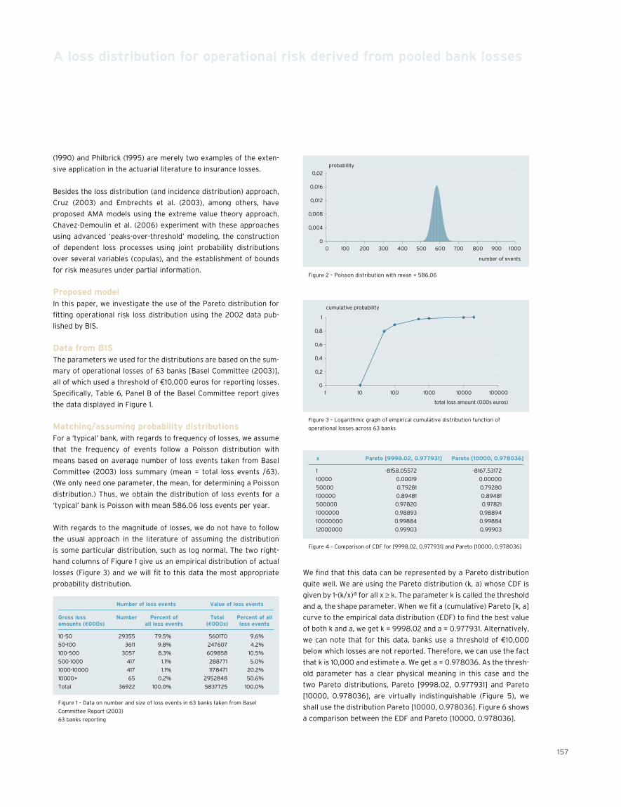
157
A loss distribution for operational risk derived from pooled bank losses
(1990) and Philbrick (1995) are merely two examples of the exten-
sive application in the actuarial literature to insurance losses.
Besides the loss distribution (and incidence distribution) approach,
Cruz (2003) and Embrechts et al. (2003), among others, have
proposed AMA models using the extreme value theory approach.
Chavez-Demoulin et al. (2006) experiment with these approaches
using advanced ‘peaks-over-threshold’ modeling, the construction
of dependent loss processes using joint probability distributions
over several variables (copulas), and the establishment of bounds
for risk measures under partial information.
Proposed modelIn this paper, we investigate the use of the Pareto distribution for
fitting operational risk loss distribution using the 2002 data pub-
lished by BIS.
Data from BIsThe parameters we used for the distributions are based on the sum-
mary of operational losses of 63 banks [Basel Committee (2003)],
all of which used a threshold of €10,000 euros for reporting losses.
Specifically, Table 6, Panel B of the Basel Committee report gives
the data displayed in Figure 1.
Matching/assuming probability distributionsFor a ‘typical’ bank, with regards to frequency of losses, we assume
that the frequency of events follow a Poisson distribution with
means based on average number of loss events taken from Basel
Committee (2003) loss summary (mean = total loss events /63).
(We only need one parameter, the mean, for determining a Poisson
distribution.) Thus, we obtain the distribution of loss events for a
‘typical’ bank is Poisson with mean 586.06 loss events per year.
With regards to the magnitude of losses, we do not have to follow
the usual approach in the literature of assuming the distribution
is some particular distribution, such as log normal. The two right-
hand columns of Figure 1 give us an empirical distribution of actual
losses (Figure 3) and we will fit to this data the most appropriate
probability distribution.
We find that this data can be represented by a Pareto distribution
quite well. We are using the Pareto distribution (k, a) whose CDF is
given by 1-(k/x)a for all x ≥ k. The parameter k is called the threshold
and a, the shape parameter. When we fit a (cumulative) Pareto [k, a]
curve to the empirical data distribution (EDF) to find the best value
of both k and a, we get k = 9998.02 and a = 0.977931. Alternatively,
we can note that for this data, banks use a threshold of €10,000
below which losses are not reported. Therefore, we can use the fact
that k is 10,000 and estimate a. We get a = 0.978036. As the thresh-
old parameter has a clear physical meaning in this case and the
two Pareto distributions, Pareto [9998.02, 0.977931] and Pareto
[10000, 0.978036], are virtually indistinguishable (Figure 5), we
shall use the distribution Pareto [10000, 0.978036]. Figure 6 shows
a comparison between the EDF and Pareto [10000, 0.978036].
number of loss events Value of loss events
Gross loss number Percent of Total Percent of all amounts (€000s) all loss events (€000s) loss events
10-50 29355 79.5% 560170 9.6%
50-100 3611 9.8% 247607 4.2%
100-500 3057 8.3% 609858 10.5%
500-1000 417 1.1% 288771 5.0%
1000-10000 417 1.1% 1178471 20.2%
10000+ 65 0.2% 2952848 50.6%
Total 36922 100.0% 5837725 100.0%
Figure 1 – Data on number and size of loss events in 63 banks taken from Basel
Committee Report (2003)
63 banks reporting
0
0,004
0,008
0,012
0,016
0,02
0 100 200 300 400 500 600 700 800 900 1000
probability
number of events
0
0,2
0,4
0,6
0,8
1
1 10 100 1000 10000 100000
cumulative probability
total loss amount (000s euros)
Figure 2 – Poisson distribution with mean = 586.06
Figure 3 – Logarithmic graph of empirical cumulative distribution function of
operational losses across 63 banks
x Pareto [9998.02, 0.977931] Pareto [10000, 0.978036]
1 -8158.05572 -8167.53172
10000 0.00019 0.00000
50000 0.79281 0.79280
100000 0.89481 0.89481
500000 0.97820 0.97821
1000000 0.98893 0.98894
10000000 0.99884 0.99884
12000000 0.99903 0.99903
Figure 4 – Comparison of CDF for [9998.02, 0.977931] and Pareto [10000, 0.978036]

158 – The journal of financial transformation
A loss distribution for operational risk derived from pooled bank losses
We also attempted to fit the generalized Pareto distribution but the
additional complexity of the model was not considered worthwhile
for the very slight gain in accuracy achieved — see Buch-Kromman’s
(2007) claim about having to use multiple parameters.
Adjusting for thresholdsMost banks record (and report) losses only above a threshold, i.e.,
€5000 or €10,000. In practice, they may have many losses. We
present here an approach to attempt to adjust for these unreport-
ed losses. For the BIS data, we have noted earlier that k = €10,000
for use with a Pareto distribution to model loss impact. However,
this did not account for unreported losses below €10,000. The
use of the Pareto distribution makes an adjustment quite straight-
forward because the shape parameter a remains unchanged.
We simply replace k by a suitable number — smaller (if there are
unreported losses below 10,000), or larger (if the smallest loss is
above €10,000 but below €50,000 euros for the data we have).
The selected value will greatly affect the cumulative distribution
function value as seen below (Figures 7 and 8). We can now cal-
culate what percentage of the distribution lies between the new k
and 10,000. Suppose this was 15%. This means that 15% of losses
are estimated to be below 10,000 and therefore not reported. We
can then adjust the mean of the Poisson distribution representing
the number of loss events by multiplying by 1.15. This will allow for
a more accurate estimation of the 99.9th percentile of the total
loss distribution, which is used as the basis for estimating capital
requirement.
However, if we consider that the values for the EDF are observed
only above the threshold of 10,000 euros, we need to take only
the relative value of what is reported to what is unreported. To
get these, we need to subtract the value of the CDF at 10,000 and
divide by (1-CDF) at 10,000 — we are subtracting the unreported
losses and dividing by the reported losses to get relative propor-
tions. We get the values provided in Figure 9.
Thus, while the observed frequencies give us a value of the shape
parameter a, the regulator needs to determine an appropriate
value of the threshold value k to account for unreported losses. The
Pareto distribution for impact of loss events gives the regulator the
flexibility of choosing k for all losses — reported and unreported —
while using the value of 10,000 for reported losses.
Note that if the true threshold is k, the proportion of unreported
loss events is as reported in Figure 10.
This means that the proportion of unreported losses depends
rather dramatically on the value of k. However, the proportion of
total annual losses (as opposed to the loss per incident) may not be
as sensitive as we shall see through simulation.
x EDf Pareto [10000, 0.978036]
1 0 -8167.53172
10000 0 0.00000
50000 0.795 0.79280
100000 0.893 0.89481
500000 0.976 0.97821
1000000 0.987 0.98894
10000000 0.998 0.99884
12000000 1 0.99903
cumulative Distribution function – Pareto(k, a) with a=0.978036
Value (€) k = 10,000 k =1000 k =100 k = 10
x - - - -
10,000 0.0% 89.4813% 98.8936% 99.8836%
50,000 79.2804% 97.8206% 99.7707% 99.9759%
100,000 89.4813% 98.8936% 99.8836% 99.9878%
500,000 97.8206% 99.7707% 99.9759% 99.9975%
1,000,000 98.8936% 99.8836% 99.9878% 99.9987%
10,000,000 99.8836% 99.9878% 99.9987% 99.9999%
Figure 6 – Numerical comparison of EDF and CDF for Pareto [10000, 0.978036]
Figure 8 – Numerical CDF of Pareto [k, 0.978036] for k = 1, 100, 1000 or 10000
0
0,2
0,4
0,6
0,8
1
1 10 100 1000 10000 100000
EDF
Pareto [10000,0.978036]
cumulative probability
x (total loss amount, 000s euro)
00,1
0,20,30,40,50,60,70,80,9
1
1 100 10000 1000000 100000000
Pareto [1,0.978036]
Pareto [100,0.978036]
Pareto [1000,0.978036]
Pareto [10000,0.978036]
cdf(x)
x
Figure 5 – Comparison of EDF and CDF for Pareto [10000, 0.978036]
Figure 7 – Graphical CDF of Pareto [k, 0.978036] for k = 1, 100, 1000 and 10000

159
A loss distribution for operational risk derived from pooled bank losses
simulation of total annual lossesTaking the number of events to be a Poisson distribution (with
586.06 events/year mean) for ‘typical’ bank, and the loss per event
as determined above to be Pareto (13146.8, 0.98706), we can gen-
erate the total annual losses.
Figures 11 and 12 provide results of annual losses over 10,000 years
for this ‘typical’ bank.
For this total annual loss distribution, we can compile statistics
like those of the BIS data. Again, keep in mind that these are total
annual losses, not the range of losses per incident.
conclusionThe Basel II accord introduced a broad framework to force banks to
quantify operational risk measurement to calculate capital reserve
requirements, but provided the flexibility to allow banks to pursue
different modeling approaches. This has been a challenge because
of paucity of a long enough history of data for any one bank to
claim to have developed a reasonable loss model without heroic
leaps of faith. We presented empirical evidence that the probability
distribution of losses, at least from the regulator’s viewpoint, is a
Pareto distribution when pooling the loss experience of the various
banks under its oversight. Indeed, the regulator has (or can have)
access to data on operational losses from all banks under its super-
vision so such a model is credible and could be a starting point for
individual banks as well.
A model based on pooled loss experience provides the regulator a
useful tool not only for regulatory approval but also for monitoring
year-on-year changes to the operational risk loss profile for banks
under the regulator’s supervision.
Further work is needed on at least three fronts. First, we could
develop means to modify results from the model for ‘typical’ bank
into a more tailored, informed recommendation for a specific bank.
Second, we could extend this work so that the model provides
bounds which can act as an ‘approved zone’ when comparing with
an individual bank’s proposed AMA results. Third, and this merits
much discussion, we need to investigate further the idea that the
regulator should stick to developing AMA models and providing
percentage guidelines to individual banks while the banks them-
selves could then focus exclusively on the risk management process
rather than developing AMA models.
10 000 20000 30000 40 000 50000
50
100
150
200
250
300
350
20 000 40 000 60 000 80 000 100 000
100
200
300
400
500
600
100 000 200000 300 000 400 000 500000
500
1000
1500
2000
200 000 400 000 600 000 800 000 1 000 000
500
1000
1500
2000
2500
3000
EDf – Pareto (k,a) with a=0.978036 with threshold 10000
Value (€) k = 10,000 k = 1000 k = 100 k = 10
x - - - -
10,000 0.0% 0.0% 0.0% 0.0%
50,000 79.2804% 79.2804% 79.2804% 79.2804%
100,000 89.4813% 89.4813% 89.4813% 89.4813%
500,000 97.8206% 97.8206% 97.8206% 97.8206%
1,000,000 98.8936% 98.8936% 98.8936% 98.8936%
10,000,000 99.8836% 99.8836% 99.8836% 99.8836%
Gross loss number Proportion cumulative amounts (€000) of years of years
10-50 7264 72.64% 72.64%
50-100 1388 13.88% 86.52%
100-500 1078 10.78% 97.30%
500-1000 138 1.38% 98.68%
1000-10000 117 1.17% 99.85%
10000+ 15 0.15% 100.00%
Total 10000 100.00%
k > 10,000 k = 10,000 k = 1000 k = 100 k = 10
0.0% 0.0% 89.4813% 98.8936% 99.8836%
statistic simulated result
Mean 217,584
Median 26,701
Max 1,031,420,000
Min 13,149
99th percentile 1,216,880
99.9th percentile 12,024,500
Standard deviation 10,354,600
Figure 12 – Simulated total loss distribution displayed with different x-axes
Figure 9 – EDF expressed as relative values of Pareto (10000, 0.978036)
Figure 13 – Distribution of total losses for simulated loss distribution
Figure 10 – Proportion of unreported losses for different threshold values
Figure 11 – Results of simulation model

160 – The journal of financial transformation
A loss distribution for operational risk derived from pooled bank losses
references• Alexander, C., 2003, Operational risk: regulation, analysis and management, Financial
Times Prentice-Hall
• Basel Committee, 2003, “The 2002 loss data collection exercise for operational risk:
summary of the data collected, Risk Management Group, Basel Committee on Banking
Supervision, Bank for International Settlements
• Beans, K. M., 2007, “Chief operational risk officers discuss Basel II and the develop-
ment of the operational risk discipline,” RMA Journal, 89:9, 8-16
• Borlaug, D., S. Fathpour, and B. Jalali, 2008, “Extreme value statistics and the Pareto
distribution in Silicon Photonics,” www.arxiv.org/ftp/arxiv/papers/0809/0809.2565.
• Buch-Kromann, T., M. Englund, J. Nielsen, J. Perch, and F. Thuring, 2007, “Non-
parametric estimation of operational risk losses adjusted for under-reporting,”
Scandinavian Actuarial Journal, 4, 293-304
• Castillo, E., and A. S. Hadi, 1997, “Fitting the generalized Pareto distribution to data,”
Journal of the American Statistical Association, 92:440, 1609-1620
• Chavez-Demoulin, V., P. Embrechts, and J. Neslehova, 2006, “Quantitative models
for operational risk: extremes, dependence and aggregation,” Journal of Banking and
Finance, 30, 2635-2658
• Cowell, R. G., R. J. Verrall and Y. K. Yoon, 2007, “Modelling operational risk with
Bayesian networks,” Journal of Risk and Insurance, 74:4, 795-827
• Cruz, M., 2003, Modeling, measuring and hedging operational risk, Wiley
• Embrechts, P., C. Kluppelberg, and T. Mikosch, 1997, Modelling extremal events for
insurance and finance, Springer
• Embrechts, P., H. Furrer, and R. Kaufmann, 2003, “Quantifying regulatory capital for
operational risk,” Derivative Use, Trading and Regulation, 9:3, 217-233
• Guillen, M., J. Gustafsson, J. P. Nielsen, and P. Pritchard, 2007, “Using external data in
operational risk,” Geneva Papers on Risk and Insurance – Issue and Practice, 32:2, 178-
189
• Holmes, M., 2003, “Measuring operational risk: a reality check,” Risk, 16:9, 84-87
• Ling, T. M., 2008, “Basel II facing talent, data shortage” The Edge Financial Daily, 5
June
• McNeil, A. J., R. Frey, and P. Embrechts, 2005, Quantitative risk management,
Princeton
• Philbrick, S.W., 1985, “A practical guide to the single parameter Pareto distribution,”
Proceedings of the Casualty Actuarial Society
• Roy, S., 2008, “Operational risk capital in banks: migrating to advanced measurement
approach,” The Hindu Business Line, 15 July
• Rytgaard, M., 1990, “Estimation in the Pareto distribution,” Astin Bulletin, 20:2, 201-216
• Scandizzo, S., 2005, “Risk mapping and key risk indicators in operational risk manage-
ment,” Economic Notes by Banca Monte dei Paschi di Siena SpA, 34:2, 231-256
• Smithson, C., and P. Song, 2004, “Quantifying operational risk,” Risk, 17:7, 57-59


162 – The journal of financial transformation
Manuscript guidelines
All manuscript submissions must be in English.
Manuscripts should not be longer than 7,000 words each. The maximum number of A4 pages allowed is 14, including all footnotes, references, charts and tables.
All manuscripts should be submitted by e-mail directly to the [email protected] in the PC version of Microsoft Word. They should all use Times New Roman font, and font size 10.
Where tables or graphs are used in the manuscript, the respective data should also be provided within a Microsoft excel spreadsheet format.
The first page must provide the full name(s), title(s), organizational affiliation of the author(s), and contact details of the author(s). Contact details should include address, phone number, fax number, and e-mail address.
Footnotes should be double-spaced and be kept to a minimum. They should be numbered consecutively throughout the text with superscript Arabic numerals.
for monographsAggarwal, R., and S. Dahiya, 2006, “Demutualization and cross-country merger of exchanges,” Journal of Financial Transformation, Vol. 18, 143-150
for booksCopeland, T., T. Koller, and J. Murrin, 1994, Valuation: Measuring and Manag-ing the Value of Companies. John Wiley & Sons, New York, New York
for contributions to collective worksRitter, J. R., 1997, Initial Public Offerings, in Logue, D. and J. Seward, eds., Warren Gorham & Lamont Handbook of Modern Finance, South-Western Col-lege Publishing, Ohio
for periodicalsGriffiths, W. and G. Judge, 1992, “Testing and estimating location vectors when the error covariance matrix is unknown,” Journal of Econometrics 54, 121-138
for unpublished materialGillan, S. and L. Starks, 1995, Relationship Investing and Shareholder Activ-ism by Institutional Investors. Working Paper, University of Texas
Guidelines for manuscript submissions
Guidelines for authors
In order to aid our readership, we have established some guidelines to ensure that published papers meet the highest standards of thought leader-ship and practicality. The articles should, therefore, meet thefollowing criteria:
1. Does this article make a significant contribution to this field of research? 2. Can the ideas presented in the article be applied to current business mod-
els? If not, is there a road map on how to get there.3. Can your assertions be supported by empirical data?4. Is my article purely abstract? If so, does it picture a world that can exist in
the future?5. Can your propositions be backed by a source of authority, preferably
yours?6. Would senior executives find this paper interesting?
subjects of interestAll articles must be relevant and interesting to senior executives of the lead-ing financial services organizations. They should assist in strategy formula-tions. The topics that are of interest to our readership include:
• Impact of e-finance on financial markets & institutions• Marketing & branding• Organizational behavior & structure• Competitive landscape• Operational & strategic issues• Capital acquisition & allocation• Structural readjustment• Innovation & new sources of liquidity • Leadership • Financial regulations• Financial technology
Manuscript submissions should be sent toShahin Shojai, Ph.D.The [email protected]
CapcoBroadgate West9 Appold StreetLondon EC2A 2APTel: +44 207 426 1500Fax: +44 207 426 1501

163
The world of finance has undergone tremendous change in recent years. Physical barriers have come down and organizations are finding it harder to maintain competitive advantage within today’s truly global market place. This paradigm shift has forced managers to identify new ways to manage their operations and finances. The managers of tomorrow will, therefore, need completely different skill sets to succeed.
It is in response to this growing need that Capco is pleased to publish the ‘Journal of financial transformation.’ A journal dedicated to the advancement of leading thinking in the field of applied finance.
The Journal, which provides a unique linkage between scholarly research and business experience, aims to be the main source of thought leadership in this discipline for senior executives, management consultants, academics, researchers, and students. This objective can only be achieved through relentless pursuit of scholarly integrity and advancement. It is for this reason that we have invited some of the world’s most renowned experts from academia and business to join our editorial board. It is their responsibility to ensure that we succeed in establishing a truly independent forum for leading thinking in this new discipline.
You can also contribute to the advancement of this field by submitting your thought leadership to the Journal.
We hope that you will join us on our journey of discovery and help shape the future of finance.
Shahin [email protected]
request for papers — Deadline July 2, 2009
For more info, see opposite page
2009 The Capital Markets Company. VU: Shahin Shojai,
Prins Boudewijnlaan 43, B-2650 Antwerp
All rights reserved. All product names, company names and registered trademarks in
this document remain the property of their respective owners.

Design, production, and coordination: Cypres — Daniel Brandt and Pieter Vereertbrugghen
© 2009 The Capital Markets Company, N.V.
All rights reserved. This journal may not be duplicated in any way without the express
written consent of the publisher except in the form of brief excerpts or quotations for review
purposes. Making copies of this journal or any portion there of for any purpose other than
your own is a violation of copyright law.