jose blanchet yang kang karthyek murthy columbia … wasserstein profile inference and applications...
TRANSCRIPT

ROBUST WASSERSTEIN PROFILE INFERENCE AND APPLICATIONS TO
MACHINE LEARNING
Jose Blanchet Yang Kang Karthyek Murthy
Columbia University
Abstract. We introduce RWPI (Robust Wasserstein Profile Inference), a novel class of sta-tistical tools which exploits connections between Empirical Likelihood, Distributionally RobustOptimization and the Theory of Optimal Transport (via the use of Wasserstein distances). Akey element of RWPI is the so-called Robust Wasserstein Profile function, whose asymptoticproperties we study in this paper. We illustrate the use of RWPI in the context of machinelearning algorithms, such as the generalized LASSO (Least Absolute Shrinkage and Selection)and regularized logistic regression, among others. For these algorithms, we show how to op-timally select the regularization parameter without the use of cross validation. The use ofRWPI for such optimal selection requires a suitable distributionally robust representation forthese machine learning algorithms, which is also novel and of independent interest. Numericalexperiments are also given to validate our theoretical findings.
1. Introduction
The goal of this paper is to introduce and investigate a novel inference methodology whichwe call RWPI (Robust Wasserstein-distance Profile-based Inference – pronounced similar toRupee1). RWPI combines ideas from three different areas: Empirical Likelihood (EL), Distri-butionally Robust Optimization, and the Theory of Optimal Transport. While RWPI can beapplied to a wide range of inference problems, in this paper we use several well known algorithmsin machine learning to illustrate the use and implications of this methodology.
We will explain, by means of several examples of interest, how RWPI can be used to optimallychoose the regularization parameter in machine learning applications without the need of crossvalidation. The examples of interest that we study in this paper include generalized LASSO(Least Absolute Shrinkage and Selection) and Regularized Logistic Regression, among others.
In order to explain RWPI let us walk through a simple application in a familiar context,namely, that of linear regression.
1.1. RWPI for optimal regularization of generalized LASSO. Consider a given a set oftraining data (X1, Y1), . . . , (Xn, Yn). The input Xi ∈ Rd is a vector of d predictor variables,and Yi ∈ R is the response variable. (Throughout the paper any vector is understood to be acolumn vector and the transpose of x is denoted by xT .) It is postulated that
Yi = βT∗ Xi + ei,
for some β∗ ∈ Rd and errors e1, ..., en. Under suitable statistical assumptions (such as indepen-dence of the samples in the training data) one may be interested in estimating β∗. Underlying
1The acronym RWPI is chosen to sound just as RUPI (”u” as in put and ”i” as in bit). In turn, RUPI meansbeautiful in Sanskrit.
1
arX
iv:1
610.
0562
7v2
[m
ath.
ST]
25
Feb
2017
2 BLANCHET, KANG AND MURTHY
there is a general loss function, l (x, y;β), which we shall take for simplicity in this discussion
to be the quadratic loss, namely, l(x, y;β) =(y − βTx
)2.
Now, let Pn be the empirical distribution function, namely,
Pn (dx, dy) :=1
n
n∑i=1
δ(Xi,Yi)(dx, dy).
Throughout out the paper we use the notation EP [·] to denote expectation with respect to aprobability distribution P .
In the last two decades, regularized estimators have been introduced and studied. Manyof them have gained substantial popularity because of their good empirical performance andinsightful theoretical properties, (see, for example, [41] for an early reference and [16] for adiscussion on regularized estimators). One such regularized estimator, implemented, for examplein the “flare” package, see [19], is the so-called generalized LASSO estimator; which is obtainedby solving the following convex optimization problem in β
(1) minβ∈Rd
√EPn [l (X,Y ;β)] + λ ‖β‖1
= min
β∈Rd
√√√√ 1
n
n∑i=1
l (Xi, Yi;β) + λ ‖β‖1
,
where ‖β‖p denotes the p-th norm in the Euclidean space. The parameter λ, commonly referredto as the regularization parameter, is crucial for the performance of the algorithm and it is oftenchosen using cross validation.
1.1.1. Distributionally robust representation of generalized LASSO . We shall illustrate how tochoose λ, satisfying a natural optimality criterion, as the quantile of a certain object whichwe call the Robust Wasserstein Profile (RWP) function evaluated at β∗. This will motivatea systematic study of the RWP function as the sample size, n, increases. However, before wedefine the associated RWP function, we first introduce a class of representations which are ofindependent interest and which are necessary to motivate the definition of the RWP functionfor choosing λ.
One of our contributions in this paper (see Section 3) is a representation of (1) in terms ofa Distributionally Robust Optimization formulation. In particular, we construct a discrepancymeasure, Dc (P,Q), based on a suitable Wasserstein-type distance, between two probabilitymeasures P and Q satisfying that
(2) minβ∈Rd
√EPn [l (X,Y ;β)] + λ ‖β‖1
2= min
β∈Rdmax
P : Dc(P,Pn)≤δEP [l(X,Y ;β)] ,
where δ = λ1/2. Observe that the regularization parameter is fully determined by the size ofthe uncertainty, δ, in the distributionally robust formulation on the right hand side of (2).
The set Uδ(Pn) = P : Dc(P, Pn) ≤ δ is called the uncertainty set in the language ofdistributionally robust optimization, and it represents the class of models that are, in somesense, plausible variations of Pn.
For every selection P in Uδ(Pn), there is an optimal choice β = β (P ) which minimizes therisk EP [l(X,Y ;β)]. We shall define Λn (δ) = β (P ) : P ∈ Uδ (Pn) to be the set of plausibleselections of the parameter β.
Now, for the definition of Λn (δ) to be sensible, we must have that the estimator obtainedfrom the left hand side of (2) is plausible. This follows from the following result, which is

RWPI AND APPLICATIONS TO MACHINE LEARNING 3
established with the aid of a min-max theorem in Section 4,
minβ∈Rd
maxP : Dc(P,Pn)≤δ
EP [l(X,Y ;β)] = minβ∈Λn(δ)
maxP : Dc(P,Pn)≤δ
EP [l(X,Y ;β)] .
Then, we will say that β∗ is plausible with (1− α) confidence, or simply, (1− α)-plausibleif δ is large enough so that β∗ ∈ Λn (δ) with probability at least 1− α. This definition leads usto the optimality criterion that we shall consider.
Our optimal selection criterion for δ is formulated as follows: Choose δ > 0 as smallas possible in order to guarantee that β∗ is plausible with (1− α) confidence.
As an additional desirable property, we shall verify that if β∗ is (1− α)-plausible, then Λn (δ)is a (1−α)-confidence region for β∗. A computationally efficient procedure for evaluating Λn (δ)will be studied in future work. Our focus in this paper is on the optimal selection of δ.
1.1.2. The associated Wasserstein Profile Function . In order to formally setup an optimizationproblem for the choice of δ > 0, note that for any given P , by convexity, any optimal selectionβ is characterized by the first order optimality condition, namely,
(3) EP[(Y − βTX
)X]
= 0.
We then introduce the following object, which is the RWP function associated with the esti-mating equation (3),
(4) Rn (β) = infDc (P, Pn) : EP
[(Y − βTX
)X]
= 0.
Finally, we claim that the optimal choice of δ is precisely the 1−α quantile, χ1−α, of Rn (β∗);that is
χ1−α = infz : P (Rn (β∗) ≤ z) ≥ 1− α
.
To see this note that if δ > χ1−α then indeed β∗ is plausible with probability at least 1 − α,but δ is not minimal. In turn, note that Rn (β) allows to provide an explicit characterizationof Λn (χ1−α),
Λn (χ1−α) = β : Rn (β) ≤ χ1−α.Moreover, we clearly have
P (β∗ ∈ Λn (χ1−α)) = P (Rn (β∗) ≤ χ1−α) = 1− α,
so Λn (χ1−α) is a (1− α)-confidence region for β∗.
In order to further explain the role of Rn(β∗), let us define Popt to be the set of probability
measures, P , supported on a subset of Rd × R for which (3) holds with β = β∗. Formally,
Popt :=P : EP
[(Y − βT∗ X
)X]
= 0.
In simple words, Popt is the set of probability measures for which β∗ is an optimal risk mini-mization parameter. Observe that using this definition we can write
Rn(β∗) = infDc(P, Pn) : P ∈ Popt.
Consequently, the set
P : Dc(P, Pn) ≤ Rn(β∗)denotes the smallest uncertainty region around Pn (in terms of Dc) for which one can find adistribution P satisfying the optimality condition EP
[(Y − βT∗ X)X
]= 0, see Figure 1 for a
pictorial representation of Popt.

4 BLANCHET, KANG AND MURTHY
Figure 1. Illustration of RWP function evaluated at β∗
In summary, Rn(β∗) denotes the smallest size of uncertainty that makes β∗ plausible. If wewere to choose a radius of uncertainty smaller than Rn(β∗), then no probability measure in theneighborhood will satisfy the optimality condition EP
[(Y − βT∗ X)X
]= 0. On the other hand,
if δ > Rn(β∗), the set P : EP
[(Y − βT∗ X)
]= 0,Dc
(P, Pn
)≤ δ
is nonempty. Given the importance of Rn(β∗) in the optimal selection of the regularizationparameter λ, if is of interest to analyze its asymptotic properties as n→∞.
It is important to note, however, that the estimating equations given in (3) are just oneof potentially many ways in which β∗ can be characterized. In the case of Gaussian inputthere is a (well known) intimate connection between (3) an maximum likelihood estimation. Ingeneral it appears sensible, at least from the standpoint of philosophical consistency to connectthe choice of estimating equation with the loss function l (x, y;β) used in the DistributionallyRobust Representation (2).
1.2. A broad perspective of our contributions. The previous discussion in the context oflinear regression highlights two key ideas: a) the RWP function as a key object of analysis, andb) the role of distributionally robust representation of regularized estimators.
The RWP function can be applied much more broadly than in the context of regularizedestimators. This paper is written with the goal of studying the RWP function for estimatingequations generally and systematically. We showcase the study of the RWP function in a con-text of great importance, namely, the optimal selection of regularization parameters in severalmachine learning algorithms.
Broadly speaking, RWPI is a statistical tool which consists in building a suitable RWPfunction in order to estimate a parameter of interest. From a philosophical standpoint, RWPIborrows heavily from Empirical Likelihood (EL), introduced in the seminal work of [23, 24].There are important methodological differences, however, as we shall discuss in the sequel. Inthe last three decades, there have been a great deal of successful applications of EmpiricalLikelihood for inference [25, 46, 7, 17, 29]. In principle all of those applications can be revisitedusing the RWP function and its ramifications. Therefore, we spend the first part of the paper,namely Section 2, discussing general properties of the RWP function.
The application of RWPI for the optimal selection of regularization parameters in variousmachine learning settings is given in Section 4. Once a suitable RWP function is obtained,

RWPI AND APPLICATIONS TO MACHINE LEARNING 5
the results in Section 4 are obtained directly from applications of our results in Section 2. Inorder to obtain the correct RWP function formulation for each of the machine learning settingsof interest, however, we will need to derive a suitable distributionally robust representationswhich, analogous to those discussed in the generalized LASSO setting. These representationsare given in Section 3 of this paper.
We now provide a more precise description of our contributions:
A) We provide general limit theorems for the asymptotic distribution (as the sample sizeincreases) of the RWP function defined for general estimating equations, not only those arisingfrom linear regression problems. Hence, providing tools to apply RWPI in substantial generality(see the results in Section 2.4).
B) We will explain how, by judiciously choosing Dc (·), we can define a family of regularizedregression estimators (See Section 3). In particular, we will show how generalized LASSO (seeand Theorem 2), and regularized logistic regression (see Theorem 3) arise as a particular caseof a RWPI formulation.
C) The results in B) allow to obtain the appropriate RWP function to select an optimalregularization parameter. We then will illustrate how to analyze the distribution of Rn (β∗)using our results form A) (see Section 4).
D) We analyze our regularization selection in the high-dimensional setting for generalizedLASSO. Under standard regularity conditions, we show (see Theorem 6) that the regularizationparameter λ might be chosen as,
λ =π
π − 2
Φ−1 (1− α/2d)√n
,
where Φ (·) is the cumulative distribution of the standard normal random variable and 1− α isa user-specified confidence level. The behavior of λ as a function of n and d is consistent withregularization selections studied in the literature motivated by different considerations.
E) We analyze the empirical performance of RWPI for the selection of the optimal regulariza-tion parameter in the context of generalized LASSO. This is done in Section 5 of the paper. Weapply our analysis both to simulated and real data and compare against the performance of crossvalidation. We conclude that our approach is comparable (not worst) than cross validation.
We now provide a discussion on topics which are related to RWPI.
1.3. Connections to related inference literature. Le us first discuss the connections be-tween RWPI and EL. In EL one builds a Profile Likelihood for an estimating equation. Forinstance, in the context of EL applied to estimating β satisfying (3), one would build a ProfileLikelihood Function in which the optimization object is only defined as the likelihood (or thelog-likelihood) between a given distribution P with respect to Pn. Therefore, the analogue ofthe uncertainty set P : Dc(P, Pn) ≤ δ, in the context of EL, will typically contain distribu-tions whose support coincides with that of Pn. In contrast, the definition of the RWP functiondoes not require the likelihood between an alternative plausible model P , and the empirical

6 BLANCHET, KANG AND MURTHY
distribution, Pn, to exist. Owing to this flexibility, for example, we are able to establish theconnection between regularization estimators and a suitable profile function.
There are other potential benefits of using a profile function which does not restrict thesupport of alternative plausible models. For example, it has been observed in the literaturethat in some settings EL might exhibit low coverage [26, 9, 43]. It is not the goal of this paperto examine the coverage properties of RWPI systematically, but it is conceivable that relaxingthe support of alternative plausible models, as RWPI does, can translate into desirable coverageproperties.
From a technical standpoint, the definition of the Profile Function in EL gives rise to a finitedimensional optimization problem. Moreover, there is a substantial amount of smoothness inthe optimization problems defining the EL Profile Function. This degree of smoothness can beleveraged in order to obtain the asymptotic distribution of the Profile Function as the samplesize increases. In contrast, the optimization problem underlying the definition of RWP functionin RWPI is an infinite dimensional linear program. Therefore, the mathematical techniquesrequired to analyze the associated RWP function are different (more involved) than the oneswhich are commonly used in the EL setting.
A significant advantage of EL, however, is that the limiting distribution of the associatedProfile Function is typically chi-squared. Moreover, such distribution is self-normalized in thesense that no parameters need to be estimated from the data. Unfortunately, this is typicallynot the case in the case of RWPI. In many settings, however, the parameters of the distributioncan be easily estimated from the data itself.
Another set of tools, strongly related to RWPI, have also been studied recently by the nameof SOS (Sample-Out-of-Sample) inference [5]. In this setting, also a RWP function is built, butthe support of alternative plausible models is assumed to be finite (but not necessarily equalto that of Pn). Instead, the support of alternative plausible models is assumed to be generatednot only by the available data, but additional samples coming from independent distributions(defined by the user). The mathematical results obtained for the RWP function in the contextof SOS are different from those obtained in this paper. For example, in the SOS setting, therates of convergence are dimension-dependent, which is not the case in the RWPI case.
1.4. Some connections to Distributionally Robust Optimization and Optimal Trans-port. Connection between robust optimization and regularization procedures such as LASSOand Support Vector Machines have been studied in the literature, see [44, 45]. The methodsproposed here differ subtly: While the papers [44, 45] add deterministic perturbations of acertain size to the predictor vectors X to quantify uncertainty, the Distributionally RobustRepresentations that we derive measure perturbations in terms of deviations from the empir-ical distribution. While this change may appear cosmetic, it brings a significant advantage:measuring deviations from empirical distribution, in turn, lets us derive suitable limit laws (or)probabilistic inequalities that can be used to choose the size of uncertainty, δ, in the uncertaintyregion Uδ(Pn) = P : Dc(P, Pn) ≤ δ.
Now, it is intuitively clear that as the number of samples n increase, the deviation of theempirical distribution from the true distribution decays to zero, as a function of n, at a specificrate of convergence. To begin with, one can simply use, as a direct approach to choosingthe size of δ, a concentration inequality that measures this rate of convergence. Such simplespecification of the size of uncertainty, suitably as a function of n, does not arise naturally inthe deterministic robust optimization approach. For a concentration inequality that measures
RWPI AND APPLICATIONS TO MACHINE LEARNING 7
such deviations in terms of the Wasserstein distance, we refer to [13] and references there in.For an application of these concentration inequalities to choose the size of uncertainty set inthe context of distributionally robust logistic regression, refer [35]. It is important to note that,despite imposing severe tail assumptions, these concentration inequalities dictate the size ofuncertainty to decay at the rate O(n−1/d); unfortunately, this prescription scales non-graciouslyas the number of dimensions increase. Since most of the modern learning problems have hugenumber of covariates, application of such concentration inequalities with poor rate of decay withdimensions may not be most suitable for applications.
In contrast to directly using concentration inequalities, the prescription that we advocatetypically has a rate of convergence of order O
(n−1/2
)as n → ∞ (for fixed d). Moreover, as
we discuss in the case of LASSO, according to our results corresponding to contribution E),our prescription of the size of uncertainty actually can be shown (under suitable regularity
conditions) to decay at rate O(√
log d/n) (uniformly over d and n), which is in agreementwith the findings of compressed sensing and high-dimensional statistics literature (see [8, 20,3] and references therein). Interestingly, the regularization parameter prescribed by RWPImethodology is automatically obtained without looking into the data (unlike cross-validation).
Although we have focused our discussion on the context of regularized estimators, our resultsare directly applicable to the area of data-driven Distributionally Robust Optimization wheneverthe uncertainty sets are defined in terms of a Wasserstein distance or, more generally, an optimaltransport metric. In particular, consider a given distributionally robust formulation of the form
minθ:G(θ)≤0
maxP : Dc(P,Pn)≤δ
EP [H(W, θ)] ,
for a random element W and a convex function H(W, ·) defined over a convex region θ :G (θ) ≤ 0 (assuming G : Rd → R convex). Here Pn is the empirical measure of the sampleW1, ...,Wn. One can then follows a reasoning parallel to what we advocate throughout ourLASSO discussion.
Argue, by applying the corresponding KKT (Karush-Kuhn-Tucker) conditions, if possible,that an optimal solution θ∗ to the problem
minθ:G(θ)≤0
EPtrue [H (W, θ)]
satisfies a system of estimating equations of the form
(5) EPtrue [h (W, θ∗)] = 0,
for a suitable h (·) (where Ptrue is the weak limit of the empirical measure Pn as n→∞).
Then, given a confidence level 1−α, one should choose δ as the (1−α) quantile of the RWPfunction function
Rn (θ∗) = infDc(P, Pn) : EP [h (W, θ∗)] = 0.The results in Section 2 can then be used directly to approximate the (1−α) quantile of Rn (θ∗).Just as we explain in our discussion of the generalized LASSO example, the selection of δ is thesmallest possible choice for which θ∗ is plausible with (1− α) confidence.
1.5. Organization of the paper. The rest of the paper is organized as follows. Section 2deals with contribution A). We first introduce Wasserstein distances. Then, we discuss theRobust Wasserstein Profile function as an inference tool in a way which is parallel to the Pro-file Likelihood in EL. We derive the asymptotic distribution of the RWP function for generalestimating equations. Section 3 corresponds to contribution B, namely, distributionally robust
8 BLANCHET, KANG AND MURTHY
representations of popular machine learning algorithms. Section 4 discusses contributions C),namely the combination of the results from contributions A) and optimal regularization param-eter selection. Our high-dimensional analysis of the RWP function in the case of generalizedLASSO is also given in Section 4. The proofs for the main results are given in Section 5. Finally,our numerical experiments using both simulated and real data set are given in Section 6.
2. The Robust Wasserstein Profile Function
Given an estimating equation EPn [h(W, θ)] = 0, the objective of this section is to study theasymptotic behavior of the associated RWP function Rn(θ). To do this, we first introduce somenotation to define optimal transport costs and Wasserstein distances. Following this, we provideevidence, initially with a simple example, followed by results for general estimating equations,that the profile function defined using Wasserstein distances is tractable.
2.1. Optimal Transport Costs and Wasserstein Distances. Let c : Rm × Rm → [0,∞]be any lower semi-continuous function such that c(u,w) = 0 if and only if u = w. Given twoprobability distributions P (·) and Q(·) supported on Rm, one can define the optimal transportcost or discrepancy between P and Q, denoted by Dc(P,Q), as
(6) Dc (P,Q) = infEπ [c (U,W )] : π ∈ P (Rm × Rm) , πU = P, πW = Q
.
Here, P (Rm × Rm) is the set of joint probability distributions π of (U,W ) supported on Rm ×Rm, and πU and πW denote the marginals of U and W under π, respectively.
Intuitively, in our formulation, the quantity c(u,w) specifies the cost of transporting unit massfrom u in Rm to another element w in Rm. As a result, the expectation Eπ[c(U,W )] denotesthe expected transport cost associated with the joint distribution π. In the sequel, Dc(P,Q),defined in (6), represents the optimal transport cost associated with probability measures Pand Q.
In addition to the stated assumptions on the cost function c(·), if c (·) is symmetric (that is,
c (u,w) = c (w, u)), and there exists ρ ≥ 1 such that c1/ρ (u,w) ≤ c1/ρ (u, z) + c1/ρ (z, w) for
all u,w, z ∈ Rm (that is, c1/ρ (·) satisfies the triangle inequality), it can be easily verified that
D1/ρc (P,Q) is a metric (see [42] for a proof, and other properties of the metric Dc).
For example, if c (u,w) = ‖u− w‖22, where ‖·‖2 is the Euclidean distance in Rm, then ρ = 2
yields that c (u,w)1/2 = ‖u− w‖2 is symmetric, non-negative, lower semi-continuous and itsatisfies the triangle inequality. In that case,
D1/2c (P,Q) = inf
√Eπ
[‖U −W‖22
]: π ∈ P (Rm × Rm) , πU = P, πW = Q
coincides with the Wasserstein distance of order two.
More generally, if we choose c1/ρ (u,w) = d (u,w) for any metric d defined on Rm, then
D1/ρc (·) is the standard Wasserstein distance of order ρ ≥ 1.
Wasserstein distances metrize weak convergence of probability measures under suitable mo-ment assumptions, and have received immense attention in probability theory (see [30, 31, 42]for a collection of classical applications). In addition, earth-mover’s distance, a particular ex-ample of Wasserstein distances, has been of interest in image processing (see [33, 38]). Morerecently, optimal transport metrics and Wasserstein distances are being actively investigated for

RWPI AND APPLICATIONS TO MACHINE LEARNING 9
its use in various machine learning applications as well (see [34, 28, 32, 37, 14, 39] and referencestherein for a growing list of new applications).
Throughout this paper, we shall select Dc for a judiciously chosen cost function c (·) informulations such as (2). It is useful to allow c (·) to be lower semi-continuous and potentiallybe infinite in some region to accommodate some of the applications, such as regularization in thecontext of logistic regression, as we shall see in Section 3. So, our setting requires discrepancychoices which are slightly more general than standard Wasserstein distances.
2.2. The RWP Function for Estimating Equations and Its Use as an Inference Tool.The Robust Wasserstein Profile function’s definition is inspired by the notion of the ProfileLikelihood function, introduced in the pioneering work of Art Owen in the context of EL (see[26]). We provide the definition of the RWP function for estimating θ∗ ∈ Rl, which we assumesatisfies
(7) E [h (W, θ∗)] = 0,
for a given random variable W taking values in Rm and an integrable function h : Rm×Rl → Rr.The parameter θ∗ will typically be unique to ensure consistency, but uniqueness is not necessaryfor the limit theorems that we shall state, unless we explicitly indicate so.
Given a set of samples W1, ...,Wn, which are assumed to be i.i.d. copies of W , we definethe Wasserstein Profile function for the estimating equation (7) as,
(8) Rn (θ) := infDc(P, Pn) : EP [h(W, θ)] = 0
.
Here, recall that Pn denotes the empirical distribution associated with the training samplesW1, . . . ,Wn and c(·) is a chosen cost function. In this section, we are primarily concernedwith cost functions of the form,
(9) c (u,w) = ‖w − u‖ρq ,
where ρ ≥ 1 and q ≥ 1. We remark, however, that the methods presented here can beeasily adapted to more general cost functions. For simplicity, we assume that the samplesW1, . . . ,Wn are distinct.
Since, as we shall see, that the asymptotic behavior of the RWP function Rn(θ) is dependenton the exponent ρ in (9), we shall sometimes write Rn (θ; ρ) to make this dependence explicit;but whenever the context is clear, we drop ρ to avoid notational burden. Also, observe that theprofile function defined in (4) for the linear regression example is obtained as a particular caseby selecting W = (X,Y ), β = θ and defining h (x, y, θ) = (y − θTx)x.
Our goal in this section is to develop an asymptotic analysis of the RWP function whichparallels that of the theory of EL. In particular, we shall establish,
(10) nρ/2Rn (θ∗; ρ)⇒ R (ρ) .
for a suitably defined random variable R (ρ) (throughout the rest of the paper, the symbol “⇒”denotes convergence in distribution).
As the empirical distribution weakly converges to the underlying probability distributionfrom which the samples are obtained from, it follows from the definition of RWP function in(10) that Rn(θ; ρ) → 0, as n → ∞, if and only if θ satisfies E[h(W, θ)] = 0; for every other θ,
we have that nρ/2Rn(θ; ρ)→∞. Therefore, the result in (10) can be used to provide confidence

10 BLANCHET, KANG AND MURTHY
regions (at least conceptually) around θ∗. In particular, given a confidence level 1− α in (0,1),if we denote ηα as the (1− α) quantile of R (ρ), that is, P
(R (ρ) ≤ ηα
)= (1− α), then
Λn
(ηαn
)=θ : Rn (θ; ρ) ≤ ηα
n
yields an approximate (1−α) confidence region for θ∗. This is because, by definition of Λn (ηα/n),we have
P(θ∗ ∈ Λn (ηα/n)
)= P
(nρ/2Rn (θ∗; ρ) ≤ ηα
)≈ P
(R (ρ) ≤ ηα
)= 1− α.
Throughout the development in this section, the dimension m of the underlying randomvector W is kept fixed and the sample size n is sent to infinity; the function h (·) can bequite general. In Section 4.3, we extend the analysis of RWP function to the case where theambient dimension could scale with the number of training samples n, in the specific contextof generalized LASSO for linear regression.
2.3. The dual formulation of RWP function. The first step in the analysis of the RWPfunction Rn(θ) is to use the definition of the discrepancy measure Dc to rewrite Rn(θ) as,
Rn(θ) = infEπ [c(U,W )] : π ∈ P (Rm × Rm) , Eπ [h (U, θ)] = 0, πW = Pn
,
which is a problem of moments of the form,
Rn(θ) = infπ∈P(Rm×Rm)
Eπ [c(U,W )] : Eπ [h (U, θ)] = 0, Eπ [I(W = Wi)] =
1
n, i = 1, n
.(11)
The problem of moments is a classical linear programming problem for which the respectivedual formulation and strong duality have been well-studied (see, for example, [18, 36]). Thelinear program problem over the variable π in (11) admits a simple dual semi-infinite linearprogram of form,
supai∈R,λ∈Rr
a0 +
1
n
n∑i=1
ai : a0 +
n∑i=1
ai1w=Wi(u,w) + λTh(u, θ) ≤ c(u,w) for ∀u,w ∈ Rm
= supλ∈Rr
1
n
n∑i=1
infu∈Rm
c(u,Wi)− λTh(u, θ)
= supλ∈Rr
− 1
n
n∑i=1
supu∈Rm
λTh(u, θ)− c(u,Wi)
.
Proposition 1 below states that strong duality holds under mild assumptions, and the dualformulation above indeed equals Rn(θ).
Proposition 1. Let h(·, θ) be Borel measurable, and Ω = (u,w) ∈ Rm × Rm : c(u,w) < ∞be Borel measurable and non-empty. Further, suppose that 0 lies in the interior of the convexhull of h(u, θ) : u ∈ Rm. Then,
Rn(θ) = supλ∈Rr
− 1
n
n∑i=1
supu∈Rm
λTh(u, θ)− c(u,Wi)
.
A proof of Proposition 1, along with an introduction to the problem of moments, is providedin Appendix A.

RWPI AND APPLICATIONS TO MACHINE LEARNING 11
2.4. Asymptotic Distribution of the RWP Function. In order to gain intuition behind(10), let us first consider the simple example of estimating the expectation θ∗ = E[W ] of areal-valued random variable W , using h (w, θ) = w − θ.
Example 1. Let h (w, θ) = w − θ with m = 1 = l = r. First, suppose that the choice of costfunction is c (u,w) = |u− w|ρ for some ρ > 1. As long as θ lies in the interior of convex hull ofsupport of W, Proposition (1) implies,
Rn(θ; ρ) = supλ∈R
− 1
n
n∑i=1
supu∈R
λ(u− θ)− |Wi − u|ρ
= supλ∈R
−λn
n∑i=1
(Wi − θ)−1
n
n∑i=1
supu∈R
λ (u−Wi)− |Wi − u|ρ
.
As max∆λ∆− |∆|ρ = (ρ− 1)|λ/ρ|ρ/(ρ−1), we obtain
Rn (θ; ρ) = supλ
−λn
n∑i=1
(Wi − θ)− (ρ− 1)
∣∣∣∣λρ∣∣∣∣ ρρ−1
=
∣∣∣∣∣ 1nn∑i=1
(Wi − θ)
∣∣∣∣∣ρ
.
Then, under the hypothesis that E [W ] = θ∗, and assuming Var[W ] = σ2W<∞, we obtain,
nρ/2Rn (θ∗; ρ)⇒ R (ρ) ∼ σρW|N (0, 1)|ρ ,
where N (0, 1) denotes a standard Gaussian random variable. The limiting distribution for thecase ρ = 1 can be formally obtained by setting ρ = 1 in the above expression for R(ρ), but theanalysis is slightly different. When ρ = 1,
Rn (θ) = supλ∈R
−λn
n∑i=1
(Wi − θ)−1
n
n∑i=1
supu∈R
λ (u−Wi)− |u−Wi|
= supλ
−λn
n∑i=1
(Wi − θ)− sup∆∈R
λ∆− |∆|
.
Following the notion that ∞× 0 = 0,
Rn(θ) = supλ
λ
n
n∑i=1
(Wi − θ)−∞I (|λ| > 1)
= max|λ|≤1
λ
n
n∑i=1
(Wi − θ) =
∣∣∣∣∣ 1nn∑i=1
(Wi − θ)
∣∣∣∣∣ .So, indeed if E[W ] = θ∗ and V ar [W ] = σ2
W<∞, we obtain
n1/2Rn (θ∗)⇒ σW |N (0, 1)| .
We now discuss far reaching extensions to the developments in Example 1 by consideringestimating equations that are more general. First, we state a general asymptotic stochasticupper bound, which we believe is the most important result from an applied standpoint as itcaptures the speed of convergence of Rn(θ∗) to zero. Following this, we obtain an asymptotic

12 BLANCHET, KANG AND MURTHY
stochastic lower bound that matches with the upper bound (and therefore the weak limit) undermild, additional regularity conditions. We discuss the nature of these additional regularityconditions, and also why the lower bound in the case ρ = 1 can be obtained basically withoutadditional regularity.
For the asymptotic upper bound we shall impose the following assumptions.
Assumptions:
A1) Assume that c (u,w) = ‖u−w‖ρq for q ≥ 1 and ρ ≥ 1. For a chosen q ≥ 1, let p be suchthat 1/p+ 1/q = 1.
A2) Suppose that θ∗ ∈ Rl satisfies E [h(W, θ∗)] = 0 and E ‖h(W, θ∗)‖22 < ∞. (While we donot assume that θ∗ is unique, the results are stated for a fixed θ∗ satisfying E[h(W, θ∗)] = 0.)
A3) Suppose that the function h(·, θ∗) is continuously differentiable with derivativeDwh(·, θ∗).
A4) Suppose that for each ζ 6= 0,
(12) P(∥∥ζTDwh (W, θ∗)
∥∥p> 0)> 0.
In order to state the theorem, let us introduce the notation for asymptotic stochastic upperbound,
nρ/2Rn(θ∗; ρ) .D R (ρ) ,
which expresses that for every continuous and bounded non-decreasing function f (·) we havethat
limn→∞E[f(nρ/2Rn(θ∗; ρ)
)]≤ E
[f(R (ρ)
)].
Similarly, we write &D for an asymptotic stochastic lower bound, namely
limn→∞E[f(nρ/2Rn(θ∗; ρ)
)]≥ E
[f(R (ρ)
)].
Therefore, if both stochastic upper and lower bounds hold, then nρ/2Rn(θ∗; ρ) ⇒ R (ρ) asn→∞. (see, for example, [4]). Now we are ready to state our asymptotic upper bound.
Theorem 1. Under Assumptions A1) to A4) we have, as n→∞,
nρ/2Rn(θ∗; ρ) .D R (ρ) ,
where, for ρ > 1,
R (ρ) := maxζ∈Rr
ρζTH − (ρ− 1)E
∥∥ζTDwh (W, θ∗)∥∥ρ/(ρ−1)
p
,
and if ρ = 1,
R (1) := maxζ:P(‖ζTDwh(W,θ∗)‖p>1)=0
ζTH.
In both cases H ∼ N (0,Cov[h(W, θ∗)]), and Cov[h(W, θ∗)] = E[h(W, θ∗)h(W, θ∗)
T].

RWPI AND APPLICATIONS TO MACHINE LEARNING 13
We remark that as ρ→ 1, one can verify that R (ρ)⇒ R (1), so formally one can simply keepin mind the expression R (ρ) with ρ > 1. In turn, it is intersting to note that R(ρ) is Fencheltransform as a function of Hn. We now study some sufficient conditions which guarantee thatR (ρ) is also an asymptotic lower bound for nρ/2Rn(θ∗; ρ). We consider the case ρ = 1 first,which will be used in applications to logistic regression discussed later in the paper.
Proposition 2. In addition to assuming A1) to A4), suppose that W has a positive density(almost everywhere) with respect to the Lebesgue measure. Then,
n1/2Rn(θ∗; 1)⇒ R (1) .
The following set of assumptions can be used to obtain tight asymptotic stochastic lowerbounds when ρ > 1; the corresponding result will be applied to the context of generalizedLASSO.
A5) (Growth condition) Assume that there exists κ ∈ (0,∞) such that for ‖w‖q ≥ 1,
(13) ‖Dwh(w, θ∗)‖p ≤ κ ‖w‖ρ−1q ,
and that E ‖Wi‖ρ <∞.
A6) (Locally Lipschitz continuity) Assume that there exists exists κ : Rm → [0,∞) suchthat,
‖Dwh(w + ∆, θ∗)−Dwh(w, θ∗)‖p ≤ κ (Wi) ‖∆‖q ,for ‖∆‖q ≤ 1, and
E [κ (Wi)c] <∞,
for c ≤ max2, ρρ−1.
We now summarize our last weak convergence result of this section.
Proposition 3. If Assumptions A1) to A6) are in force and ρ > 1, then
nρ/2Rn(θ∗; ρ)⇒ R (ρ) .
Before we move on with the applications of the previous results, it is worth discussing thenature of the additional assumptions introduced to ensure that an asymptotic lower bound canbe obtained which matches the upper bound in Theorem 1.
As we shall see in the technical development in Section 5.1 where the proofs of the aboveresults are furnished, the dual formulation of RWP function in Proposition 1 can be re-expressed,assuming only A1) to A4), as,(14)
nρ/2Rn (θ∗; ρ) = supζ
ζTHn −
1
n
n∑k=1
sup∆
∫ 1
0ζTDh
(Wi + ∆u/n1/2, θ∗
)∆du− ‖∆‖ρq
.
In order to make sure that the lower bound asymptotically matches the upper bound obtainedin Theorem 1 we need to make sure that we rule out cases in which the inner supremum is infinitein (14) with positive probability in the prelimit.
14 BLANCHET, KANG AND MURTHY
In Proposition 2 we assume that W has a positive density with respect to the Lebesguemeasure because in that case the condition
P(∥∥ζTDh (W, θ∗)
∥∥p≤ 1)
= 1,
(which appears in the upper bound obtained in Theorem 1) implies that∥∥ζTDh (w, θ∗)
∥∥p≤ 1
almost everywhere with respect to the Lebesgue measure. Due to the appearance of the integralin the inner supremum in (14), an upper bound can be obtained for the inner supremum, which
translates into a tight lower bound for nρ/2Rn (θ∗).
Moving to the case ρ > 1 studied in Proposition 3, condition (13) in A5) guarantees that (forfixed Wi and n) ∥∥∥Dh(Wi + ∆u/n1/2, θ∗
)∆∥∥∥ = O
(‖∆‖ρq /n
(ρ−1)/2),
as ‖∆‖q → ∞. Therefore, the cost term(−‖∆‖ρq
)in (14) will ensure a finite optimum in
the prelimit for large n. The condition that E ‖W‖ρq < ∞ is natural because we are using a
optimal transport cost c (u,w) = ‖u− w‖ρq . If this condition is not satisfied, then the underlyingnominal distribution is at infinite transport distance from the empirical distribution.
The local Lipschitz assumption A6) is just imposed to simplify the analysis and can berelaxed; we have opted to keep A6) because we consider it mild in view of the applications thatwe will study in the sequel.
3. Distributionally Robust Estimators for Machine Learning Algorithms
A common theme in machine learning problems is to find the best fitting parameter in a familyof parameterized models that relate a vector of predictor variables X ∈ Rd to a response Y ∈ R.In this section, we shall focus on a useful class of such models, namely, linear and logisticregression models. Associated with these models, we have a loss function l(Xi, Yi;β) whichevaluates the fit of regression coefficient β for the given data points (Xi, Yi) : i = 1, . . . , n.Then, just as we explained in the case of generalized LASSO in the Introduction, our first stepwill be to show that regularized linear and logistic regression estimators admit a DistributionallyRobust Optimization (DRO) formulation of the form,
(15) minβ∈Rd
supP :Dc
(P,Pn
)≤δEP[l(X,Y ;β
)].
Once we derive a representation such as (15) then we will proceed, in the next section to findthe optimal choice of δ, which, as explained in the Introduction, will immediately characterizethe optimal regularization parameter.
In contrast to the empirical risk minimization that performs well only on the training data,the DRO problem (15) finds an optimizer β that performs uniformly well over all probabilitymeasures in the neighborhood that can be perceived as perturbations to the empirical trainingdata distribution. Hence the solution to (15) is said to be “distributionally robust”, and canbe expected to generalize better. See [44, 45] and [35] for works that relate robustness andgeneralization.
Recasting regularized regression as a DRO problem of form (15) lets us view these regularizedestimators under the lens of distributional robustness. The regularized estimators that weconsider in this section, in particular, include the following.

RWPI AND APPLICATIONS TO MACHINE LEARNING 15
Example 2 (Generalized-LASSO). We have already started discussing this example in theIntroduction, namely given a set of training data (X1, Y1), . . . , (Xn, Yn), with predictor Xi ∈Rd and response Yi ∈ R, the postulated model is Yi = βT∗ Xi + ei for some β∗ ∈ Rd and errors
e1, ..., en. The underlying loss function is l(x, y;β) =(y − βTx
)2and the generalized LASSO
estimator, is obtained by solving the problem,
minβ∈Rd
√EPn [l (X,Y ;β)] + λ ‖β‖1
,
see [3, 1, 27] for more on generalized LASSO. As Pn denotes the empirical distribution corre-sponding to training samples, EPn [l (X,Y ;β)] is just the mean square training loss. In additionto the Generalized LASSO estimator above with `1 penalty, we derive a DRO representation ofthe form (15) for `p-penalized estimators obtained by solving,
minβ∈Rd
√EPn [l (X,Y ;β)] + λ ‖β‖p
,(16)
for any p ∈ [1,∞).
Example 3 (Regularized Logistic Regression). We next consider the context of binary classi-fication, in which case the data is of the form (X1, Y1), . . . , (Xn, Yn), with Xi ∈ Rd, responseYi ∈ −1, 1 and the model postulates that
log
(P (Yi = 1|Xi = x)
1− P (Yi = 1|Xi = x)
)= βT∗ x
for some β∗ ∈ Rd. In this case, the log-exponential loss function (or negative log-likelihood forbinomial distribution) is
l (x, y;β) = log(1 + exp(−y · βTx)
),
and one is interested in estimating β∗ by solving
(17) minβ∈Rd
EPn [l (X,Y ;β)] + λ ‖β‖p
,
for p ∈ [1,∞) (see [16] for a discussion on regularized logistic regressions).
The rest of this section is to show that generalized LASSO and Regularized Logistic Regres-sion estimators are distributionally robust (in the sense, they admit a representation of the form(15)).
While these particular examples may be certainly interesting, we emphasize that the DROformulation (15) should be viewed, in its entirety, as a framework for generating distributionallyrobust inference procedures for different models and loss functions, without having to proveequivalences with an existing or popular algorithm.
3.1. Dual form of the DRO formulation (15). Though the DRO formulation (15) involvesoptimizing over uncountably many probability measures, the following result ensures that theinner supremum in (15) over the neighborhood P : Dc(P, Pn) ≤ δ admits a reformulationwhich is a simple, univariate optimization problem. Before stating the result, we recall that thedefinition of discrepancy measure Dc (defined in (6)) requires the specification of cost functionc ((x, y), (x′, y′)) between any two predictor-response pairs (x, y), (x′, y′) ∈ Rd+1.
16 BLANCHET, KANG AND MURTHY
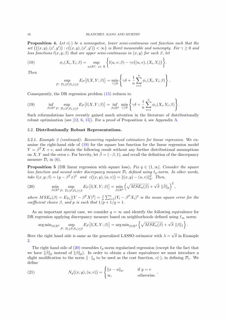
Proposition 4. Let c(·) be a nonnegative, lower semi-continuous cost function such that theset
((x, y), (x′, y′)
): c((x, y), (x′, y′)
)<∞ is Borel measurable and nonempty. For γ ≥ 0 and
loss functions l(x, y;β) that are upper semi-continuous in (x, y) for each β, let
(18) φγ(Xi, Yi;β) = supu∈Rd, v∈ R
l(u, v;β)− γc
((u, v), (Xi, Yi)
).
Then
supP : Dc(P,Pn)≤δ
EP[l(X,Y ;β)
]= min
γ≥0
γδ +
1
n
n∑i=1
φγ(Xi, Yi;β)
.
Consequently, the DR regression problem (15) reduces to
(19) infβ∈Rd
supP : Dc(P,Pn)≤δ
EP[l(X,Y ;β)
]= inf
β∈Rdminγ≥0
γδ +
1
n
n∑i=1
φγ(Xi, Yi;β)
.
Such reformulations have recently gained much attention in the literature of distributionallyrobust optimization (see [12, 6, 15]). For a proof of Proposition 4, see Appendix A.
3.2. Distributionally Robust Representations.
3.2.1. Example 2 (continued): Recovering regularized estimators for linear regression. We ex-amine the right-hand side of (19) for the square loss function for the linear regression modelY = βTX + e, and obtain the following result without any further distributional assumptionson X,Y and the error e. For brevity, let β = (−β, 1), and recall the definition of the discrepancymeasure Dc in (6).
Proposition 5 (DR linear regression with square loss). Fix q ∈ (1,∞]. Consider the squareloss function and second order discrepancy measure Dc defined using `q-norm. In other words,take l(x, y;β) = (y − βTx)2 and c
((x, y), (u, v)
)= ‖(x, y)− (u, v)‖2q. Then,
(20) minβ∈Rd
supP : Dc(P,Pn)≤δ
EP[l(X,Y ;β)
]= min
β∈Rd
(√MSEn(β) +
√δ ‖β‖p
)2,
where MSEn(β) = EPn [(Y − βTX)2] = 1n
∑ni=1(Yi − βTXi)
2 is the mean square error for thecoefficient choice β, and p is such that 1/p+ 1/q = 1.
As an important special case, we consider q = ∞ and identify the following equivalence forDR regression applying discrepancy measure based on neighborhoods defined using `∞ norm:
arg minβ∈Rd supP : Dc(P,Pn)≤δ
EP[l(X,Y ;β)
]= arg minβ∈Rd
√MSEn(β) +
√δ ‖β‖1
.
Here the right hand side is same as the generalized LASSO estimator with λ =√δ in Example
2.
The right hand side of (20) resembles `p-norm regularized regression (except for the fact thatwe have ‖β‖p instead of ‖β‖p). In order to obtain a closer equivalence we must introduce aslight modification to the norm ‖ · ‖q to be used as the cost function, c(·), in defining Dc. Wedefine
Nq
((x, y), (u, v)
)=
‖x− u‖q, if y = v
∞, otherwise.,(21)
RWPI AND APPLICATIONS TO MACHINE LEARNING 17
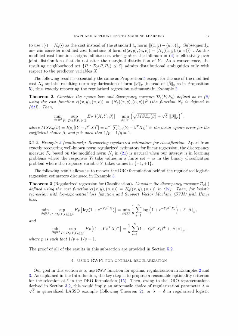
to use c(·) = Nq(·) as the cost instead of the standard `q norm ‖(x, y)− (u, v)‖q. Subsequently,one can consider modified cost functions of form c((x, y), (u, v)) = (Nq((x, y), (u, v)))a. As thismodified cost function assigns infinite cost when y 6= v, the infimum in (4) is effectively overjoint distributions that do not alter the marginal distribution of Y . As a consequence, theresulting neighborhood set P : Dc(P, Pn) ≤ δ admits distributional ambiguities only withrespect to the predictor variables X.
The following result is essentially the same as Proposition 5 except for the use of the modifiedcost Nq and the resulting norm regularization of form ‖β‖p (instead of ‖β‖p as in Proposition5), thus exactly recovering the regularized regression estimators in Example 2.
Theorem 2. Consider the square loss and discrepancy measure Dc(P, Pn) defined as in (6)using the cost function c((x, y), (u, v)) = (Nq((x, y), (u, v)))2 (the function Nq is defined in(21)). Then,
minβ∈Rd
supP : Dc(P,Pn)≤δ
EP[l(X,Y ;β)
]= min
β∈Rd
(√MSEn(β) +
√δ ‖β‖p
)2,
where MSEn(β) = EPn [(Y − βTX)2] = n−1∑n
i=1(Yi− βTXi)2 is the mean square error for the
coefficient choice β, and p is such that 1/p+ 1/q = 1.
3.2.2. Example 3 (continued): Recovering regularized estimators for classification. Apart fromexactly recovering well-known norm regularized estimators for linear regression, the discrepancymeasure Dc based on the modified norm Nq in (21) is natural when our interest is in learningproblems where the responses Yi take values in a finite set – as in the binary classificationproblem where the response variable Y takes values in −1,+1.
The following result allows us to recover the DRO formulation behind the regularized logisticregression estimators discussed in Example 3.
Theorem 3 (Regularized regression for Classification). Consider the discrepancy measure Dc(·)defined using the cost function c((x, y), (u, v)) = Nq((x, y), (u, v)) in (21). Then, for logisticregression with log-exponential loss function and Support Vector Machine (SVM) with Hingeloss,
minβ∈Rd
supP : Dc(P,Pn)≤δ
EP[
log(1 + e−Y βTX)
]= min
β∈Rd1
n
n∑i=1
log(
1 + e−YiβTXi)
+ δ ‖β‖p ,
and
minβ∈Rd
supP : Dc(P,Pn)≤δ
EP[(1− Y βTX)+
]=
1
n
n∑i=1
(1− YiβTXi)+ + δ ‖β‖p ,
where p is such that 1/p+ 1/q = 1.
The proof of all of the results in this subsection are provided in Section 5.2.
4. Using RWPI for optimal regularization
Our goal in this section is to use RWP function for optimal regularization in Examples 2 and3. As explained in the Introduction, the key step is to propose a reasonable optimality criterionfor the selection of δ in the DRO formulation (15). Then, owing to the DRO representationsderived in Section 3.2, this would imply an automatic choice of regularization parameter λ =√δ in generalized LASSO example (following Theorem 2), or λ = δ in regularized logistic

18 BLANCHET, KANG AND MURTHY
regression (following Theorem 3). In the development below, we follow the logic described inthe Introduction for the generalized LASSO setting.
We write Uδ(Pn) to denote the uncertainty set, namely Uδ(Pn) = P : Dc(P, Pn
)≤ δ, and β∗
to denote the underlying linear or logistic regression model parameter from which the trainingsamples (Xi, Yi) : i = 1, . . . , n are obtained. Now, for each P , convexity considerationsinvolving the loss functions l (x, y;β), as a function of β, will allow us to conclude that the set
Popt(β) :=P ∈ P
(Rd × R
): EP
[Dβl(X,Y ;β∗)
]= 0
is the set of probability measures for which β is an optimal risk minimization parameter.
As indicated in the Introduction, we shall say that β∗ is plausible for a given choice of δ if,
Popt(β∗) ∩ Uδ(Pn) 6= ∅.
If this intersection is empty, we say that β∗ is implausible. Moreover, we remark that β∗ isplausible with confidence at least 1− α if,
P (Popt(β∗) ∩ Uδ(Pn) 6= ∅) ≥ 1− α.
We shall argue in Appendix B that the inf sup in the corresponding DRO formulation (15)of each of the machine learning algorithms that we consider can be exchanged as below:
Lemma 1. In the settings of Theorems 2 and 3, if E‖X‖22 <∞, we have that
(22) infβ∈Rd
supP∈ Uδ(Pn)
EP[l(X,Y ;β
)]= sup
P∈ Uδ(Pn)infβ∈Rd
EP[l(X,Y ;β
)].
The representation in the right hand side of (22) implies that
supP∈ Uδ(Pn)
infβ∈Rd
EP[l(X,Y ;β
)]= sup
P∈ Uδ(Pn)
EP[l(X,Y ;β
)]: β ∈ Rd such that EP
[Dβl(X,Y ;β)
]= 0
= sup
EP[l(X,Y ;β
)]: β ∈ Rd such that Popt(β) ∩ Uδ(Pn) = ∅
,
and this motivates our interest in finding a δ such that
(23) infδ : P
(Popt(β∗) ∩ Uδ(Pn) 6= ∅
)≥ 1− α
.
asymptotically, as n → ∞. In simple words, we wish to find the smallest value of δ for whichβ∗ is plausible with at least 1− α confidence (see Figure 1).
Observe that as
Rn(β∗) = infDc(P, Pn) : P ∈ Popt(β∗)
,
we have,
P(Popt(β∗) ∩ Uδ(Pn) 6= ∅
)= P
(Rn(β∗) ≤ δ
)and therefore (23) is equivalent to
(24) infδ : P (Rn(β∗) ≤ δ) ≥ 1− α
,
thus obtaining that the optimal selection of δ as the 1− α quantile of Rn(β∗).

RWPI AND APPLICATIONS TO MACHINE LEARNING 19
Now, without knowing β∗, it is, of course, difficult to compute Rn(β∗). However, assumingi.i.d. training data, we can obtain a limiting distribution for the quantity nRn(β∗) or
√nRn(β∗),
by applying results from Section 2.4.
Another consequence of Lemma 1 is that the set Λn (δ) of plausible values of β (i.e. β forwhich there exists P ∈ Uδ(Pn) such that EP
[Dβl(X,Y ;β)
]= 0), contains the optimal solution
obtained by solving the problem in the left hand side of (22). (If this was not the case, theleft hand side in (22) would be strictly smaller than the right hand side of (22).) The fact thatthe estimator for β∗ obtained by solving the left hand side in (22) is plausible, we believe, is aproperty which makes our selection of δ logically consistent with the ultimate goal of the overallestimation procedure, namely, choosing β∗.
4.1. Linear regression models with squared loss function. In this section, we derivethe asymptotic limiting distribution of suitably scaled profile function corresponding to theestimating equation
E[(Y − βTX)X] = 0.
The chosen estimating equation describes the optimality condition for square loss functionl(x, y;β) = (y − βTx)2, and therefore, the corresponding Rn(β∗) is a suitable for choosing δ as
in (24), and the regularization parameter λ =√δ in Example 2.
Let H0 denote the null hypothesis that the training samples (X1, Y1), . . . , (Xn, Yn) areobtained independently from the linear model Y = βT∗ X + e, where the error term e has zeromean, variance σ2, and is independent of X. Let Σ = Cov[X].
Theorem 4. Consider the discrepancy measure Dc(·) defined as in (6) using the cost functionc((x, y), (u, v)) = (Nq((x, y), (u, v)))2 (the function Nq is defined in (21)). For β ∈ Rd, let
Rn(β) = infDc(P, Pn) : EP
[(Y − βTX)X
]= 0
.
Then, under the null hypothesis H0,
nRn(β∗)⇒ L1 := maxξ∈Rd
2σξTZ − E
∥∥eξ − (ξTX)β∗∥∥2
p
,
as n→∞. In the above limiting relationship, Z ∼ N (0,Σ). Further,
L1
D≤ L2 :=
E[e2]
E[e2]− (E|e|)2 ‖Z‖2q .
Specifically, if the additive error term e follows centered normally distribution, then
L1
D≤ L2 :=
π
π − 2‖Z‖2q .
In the above theorem, the relationship L1
D≤ L2 denotes that the limit law L1 is stochastically
dominated by L2. We remark this notationD≤ for stochastic upper bound here is different from
the notation .D introduced in Section 2.4 to denote asymptotic stochastic upper bound. Aproof of Theorem 4 as an application of Theorem 1 and Proposition 3 is presented in Section5.3.
Using Theorem 4 to obtain regularization parameter for (16). Let η1−α denote the(1−α) quantile of the limiting random variable L1 in Theorem 4, or its stochastic upper bound

20 BLANCHET, KANG AND MURTHY
L2. If we choose δ = η1−α/n, it follows from Theorem 4 that
P (Rn(β∗) ≤ δ) ≥ 1− α,
asymptotically as n→∞, and consequently,
P(Popt(β∗) ∩ Uδ(Pn) 6= ∅
)≥ 1− α.
In other words, the optimal regression coefficient β∗ remains plausible (for the DRO formulation(15)) with probability exceeding 1− α with this choice of δ. Due to the distributionally robustrepresentation derived in Theorem 2, a prescription for the uncertainty set size δ naturallyprovides the prescription, λ =
√δ, for the regularization parameter as well. The following steps
summarize the guidelines for choosing the regularization parameter in the `p-penalized linearregression (16):
1) Draw samples Z from N (0,Σ) to estimate the 1 − α quantile of one of the randomvariables L1 or L2 in Theorem 4. Let us use η1−α to denote the estimated quantile.While L2 is simply the norm of Z, obtaining realizations of limit law L1 involves solvingan optimization problem for each realization of Z. If Σ = Cov[X] is not known, one canuse a simple plug-in estimator for Cov[X] in place of Σ.
2) Choose the regularization parameter λ to be
λ =√δ =
√η1−α/n.
It is interesting to note that unlike the traditional LASSO algorithm, the prescription ofregularization parameter in the above procedure is self-normalizing, in the sense that it doesnot depend on the variance of e.
4.2. Logistic Regression with log-exponential loss function. In this section, we applyresults in Section 2.4 to prescribe regularization parameter for `p-penalized logistic regressionin Example 3.
Let H0 denote the null hypothesis that the training samples (X1, Y1), . . . , (Xn, Yn) are ob-tained independently from a logistic regression model satisfying
log
(P (Y = 1|X = x)
1− P (Y = 1|X = x)
)= βT∗ x,
for predictors X ∈ Rd and corresponding responses Y ∈ −1, 1; further, under null hypoth-esis H0, the predictor X has positive density almost everywhere with respect to the Lebesguemeasure on Rd. The log-exponential loss (or negative log-likelihood) that evaluates the fit of alogistic regression model with coefficient β is given by
l(x, y;β) = − log p(y|x;β) = log(1 + exp(−yβTx)
).
If we let
h(x, y;β) = Dβl(x, y;β) =−yx
1 + exp(yβTx),(25)
then the optimality condition that the coefficient β∗ satisfies is E [h(x, y;β∗)] = 0.
Theorem 5. Consider the discrepancy measure Dc(·) defined as in (6) using the cost functionc((x, y), (u, v)) = Nq((x, y), (u, v)) (the function Nq is defined in (21)). For β ∈ Rd, let
Rn(β) = infDc(P, Pn) : EP
[h(x, y;β)
]= 0
,

RWPI AND APPLICATIONS TO MACHINE LEARNING 21
where h(·) is defined in (25). Then, under the null hypothesis H0,√nRn(β∗)⇒ L3 := sup
ξ∈AξTZ
as n→∞. In the above limiting relationship,
Z ∼ N(0, E
[XXT
(1 + exp(Y βT∗ X))2
])and A =
ξ ∈ Rd : ess supx,y
∥∥ξTDxh(x, y;β)∥∥p≤ 1.
Moreover, the limit law L3 admits the following simpler stochastic bound:
L3
D≤ L4 := ‖Z‖q,
where Z ∼ N (0, E[XXT ]).
A proof of Theorem 4 as an application of Theorem 1 and Proposition 2 is presented in Section5.3.
Using Theorem 5 to obtain regularization parameter for (17) . Similar to linear re-gression, the regularization parameter for Regularized Logistic Regression discussed in Example3 can be chosen by the following procedure:
1) Estimate the (1−α) quantile of L4 := ‖Z‖q, where Z ∼ N (0, E[XXT ]). Let us use η1−αto denote the estimate of the quantile.
2) Choose the regularization parameter λ in the norm regularized logistic regression esti-mator (17) in Example 3 to be
λ = δ = η1−α/√n.
4.3. Optimal regularization in high-dimensional generalized LASSO . In this section,let us restrict our attention to the square-loss function l(x, y;β) = (y − βTx)2 for the linearregression model and the discrepancy measure Dc defined using the cost function c = Nq withq =∞ in (21). Then, due to Theorem 2, this corresponds to the interesting case of generalizedLASSO or `2-LASSO that was rather a particular example in the class of `p penalized linearregression estimators considered in Section 4.1.
As an interesting byproduct of the RWP function analysis, the following theorem presents aprescription for regularization parameter even in high dimensional settings where the ambientdimension d is larger than the number of samples n. We introduce the growth parameter,
C(n, d) :=E ‖X‖∞√
n=E [maxi=1,...,d |Xi|]√
n,
as a function of n and d, that will be useful in stating our results. In addition, we say that thepredictors X have sub-gaussian tails if there exists a constant a > 0,
E[exp(tTX)
]≤ exp(a2‖t‖2
2/2)
for every t ∈ Rd.
Theorem 6. Let E[Xi] = 0 and E[X2i ] = 1 for all i = 1, . . . , d. Suppose the assumptions of
Theorem 4 hold and assume the largest eigenvalue of Σ = Cov[X] be o(nC(n, d)2). In addition,suppose that β∗ satisfies a weak sparsity condition that ‖β∗‖1 = o(1/C(n, d)). Then
nRn(β∗) .D‖Zn‖2∞Var|e|
,

22 BLANCHET, KANG AND MURTHY
as n, d → ∞. Here, Zn := 1√n
∑ni=1 eiXi. In particular, if the predictors X have subgaussian
tails, then we have
nRn(β∗) .DEe2
Ee2 −(E|e|
)2 ‖Z‖2∞where, Z follows the distribution N (0,Σ). Moreover, if the additive error e is normally dis-tributed and Σ is the identity matrix, then the above stochastic bounds simplify to√
Rn(β∗) .Dπ
π − 2
Φ−1(1− α/2d)√n
,
with probability asymptotically larger than 1−α. Here, Φ−1(1−α) denotes the quantile x of thestandard normal distribution Φ(x) = 1− α.
The prescription of regularization parameter as
(26) λ =√δ =
π
π − 2
Φ−1(1− α/2d)√n
= O
(√log d
n
),
as in Theorem 6, is consistent with the findings in the literature of high-dimensional linearregression (see, for example, [3, 22, 46, 2] ). This agreement strengthens the interpretation of
regularization parameter in regularized regression as√Rn(β∗), which, in turn, corresponds to
the distance of the empirical distribution Pn from the set P : EP [(Y − βTX)X] = 0.It is also interesting to note that unlike traditional LASSO algorithm, the prescription of
regularization parameter as in (26) is self-normalizing, in the sense that it does not depend onthe variance of e, even if the number of predictors d is larger than n.
5. Proofs of main results
This section, comprising the proofs of the main results, is organized as follows. Subsection5.1 contains the proofs of stochastic upper and lower bounds (and hence weak limits) presentedin Section 2.4. While Subsection 5.2 is devoted to derive the results on distributionally robustrepresentations presented in Section 3.2, Subsection 5.3 contains the proofs of Theorems 4 and5 as applications of the stochastic upper and lower bounds presented in Section 2.4. Some ofthe useful technical results that are not central to the argument are presented in the appendix.
5.1. Proofs of asymptotic stochastic upper and lower bounds of RWP function inSection 2.4. We first use Proposition 1 to derive a dual formulation for nρ/2Rn(θ∗) which willbe the starting point of our analysis. Due to Assumption A2) E[h(W, θ∗)] = 0, and therefore,0 lies in the interior of convex hull of h(u, θ∗) : u ∈ Rm. Therefore, due to Proposition 1,
Rn(θ∗) = supλ∈Rr
− 1
n
n∑i=1
supu∈Rm
λTh(u, θ∗)− ‖u−Wi‖ρq
.
In order to simplify the notation, throughout the rest of the proof we will write h (Wi) insteadof h (Wi, θ∗) and Dh (Wi) for Dwh (Wi, θ∗).
Letting Hn = n−1/2∑n
i=1 h(Wi) and changing variables to ∆ = u−Wi, we obtain
Rn(θ∗) = supλ
−λT Hn
n1/2− 1
n
n∑i=1
sup∆
λT(h(Wi + ∆)− h(Wi)
)− ‖∆‖ρq
.

RWPI AND APPLICATIONS TO MACHINE LEARNING 23
Due to Fundamental calculus (using Assumption A3)), we have that
h (Wi + ∆)− h (Wi) =
∫ 1
0Dh (Wi + u∆) ∆du.
Now, redefining ζ = λn(ρ−1)/2 and ∆ = ∆/n1/2 we arrive at following representation
(27) nρ/2Rn(θ∗) = maxζ
−ζTHn −Mn (ζ)
,
where
(28) Mn (ζ) =1
n
n∑i=1
max∆
ζT∫ 1
0Dh
(Wi + n−1/2∆u
)∆du− ‖∆‖ρq
.
The reformulation in (27) is our starting point of the analysis.
To proceed further, we first state a result which will allow us to apply a localization argumentin the representation of nρ/2Rn (θ∗) in (27). Recall the definition of Mn above in (28) and that
Hn = n−1/2∑n
i=1 h(Wi).
Lemma 2. Suppose that the Assumptions A2) to A4) are in force. Then, for every ε > 0, thereexists n0 > 0 and b ∈ (0,∞) such that
P
(max‖ζ‖p≥b
−ζTHn −Mn (ζ)
> 0
)≤ ε,
for all n ≥ n0.
Proof of Lemma 2. For ζ 6= 0, we write ζ = ζ/ ‖ζ‖p. Let us define the vector Vi(ζ)
=(Dh (Wi)
T ζ)
, and put
(29) ∆′i = ∆′i(ζ)
=∣∣Vi (ζ)∣∣p/q sgn (Vi (ζ)) .
Define the set C0 = ‖Wi‖p ≤ c0, where c0 will be chosen large enough momentarily. Then, for
any c > 0, plugging in ∆ = c∆′i, we have ζTDh(Wi)∆ = c‖ζTDh(Wi)‖p‖∆′‖q, and therefore,
max∆
ζT∫ 1
0Dh
(Wi + n−1/2∆u
)∆− ‖∆‖ρq
≥ max
c∥∥ζTDh (Wi)
∥∥p
∥∥∆′i∥∥q− cρ
∥∥∆′i∥∥ρq
+ cζT∫ 1
0[Dh
(Wi + n−1/2∆′iu
)−Dh (Wi)]∆
′i, 0
I (Wi ∈ C0) .(30)
Due to Holder’s inequality,
I (Wi ∈ C0)
∣∣∣∣ζT ∫ 1
0[Dh
(Wi + n−1/2∆′iu
)−Dh (Wi)]∆
′idu
∣∣∣∣≤ ‖ζ‖p
∫ 1
0I (Wi ∈ C0)
∥∥∥[Dh(Wi + n−1/2∆′iu)−Dh (Wi)
]∆′i
∥∥∥qdu.
Because of continuity Dh (·) and the fact that Wi ∈ C0 (so the integrand is bounded), we havethat the previous expression converges to zero as n → ∞. Therefore for any ε′ > 0 (note than

24 BLANCHET, KANG AND MURTHY
convergence is uniform on Wi ∈ C0), there exists n0 such that for all n ≥ n0
(31) cI (Wi ∈ C0)
∣∣∣∣ζT ∫ 1
0[Dh
(Wi + n−1/2∆′iu
)−Dh (Wi)]∆
′idu
∣∣∣∣ ≤ cε′ ‖ζ‖p .Next, as ‖Dh(Wi)
T ζ‖p = ‖∆′i‖q/pq and q/p+ 1 = q,
c∥∥ζTDh (Wi)
∥∥p
∥∥∆′i∥∥q− cρ
∥∥∆′i∥∥ρq
= c ‖ζ‖p∥∥∆′i
∥∥qq− cρ
∥∥∆′i∥∥ρq.
Now, since ζ →∥∥∆′i
(ζ)∥∥qq
is Lipschitz continuous on∥∥ζ∥∥
p= 1, we conclude that,
1
n
n∑i=1
∥∥∆′i(ζ)∥∥qqI (Wi ∈ C0)→E
[∥∥DTwh (W ) ζ
∥∥qqI (W ∈ C0)
],
with probability one as n → ∞. Moreover, due to Fatou’s lemma we have that the map
ζ → P(∥∥ζTDwh (W )
∥∥q> 0)
is lower semi-continuous. Therefore, by A4), we have that there
exists δ > 0 such that
(32) infζE(∥∥ζTDwh (W )
∥∥2
q
)> δ,
we conclude, by selecting c0 > 0 large enough, using the equivalence between norms in Euclideanspace, we have that for n ≥ N ′ (δ), then
(33)1
n
n∑i=1
∥∥∆′i(ζ)∥∥qqI (Wi ∈ C0) >
δ
2.
Similarly, the map ζ →∥∥∆′i
(ζ)∥∥ρq
is Lipschitz continuous on∥∥ζ∥∥
q= 1, therefore one might
assume that N ′ (δ) is actually chosen so that for n ≥ N ′ (δ) ,
1
n
n∑i=1
∥∥∆′i(ζ)∥∥ρqI (Wi ∈ C0) < 2E
[∥∥∆′i(ζ)∥∥ρqI (Wi ∈ C0)
].
As ‖∆′i(ζ)‖q = ‖ζTDh(Wi)‖p/qp , and c1 := supw∈C0‖ζTDh(w)‖p <∞,
1
n
n∑i=1
∥∥∆′i(ζ)∥∥ρqI (Wi ∈ C0) < 2c
ρ pq
1 ,
for all n > N ′(δ). As a consequence, if n ≥ N ′ (δ), it follows from (30), (31) and (33) that
sup‖ζ‖p>b
−ζTHn −Mn (ζ)
≤ sup‖ζ‖p>b
−ζTHn − c
δ
2‖ζ‖p −
2cρp/q1
b− ε′ ‖ζ‖p
≤ sup‖ζ‖p>b
−ζTHn − c ‖ζ‖p
δ
2− 2c
ρp/q1
b− ε′
.
From the previous expression, on the set ‖Hn‖q ≤ b′, we have that if b ≥ 1,
sup‖ζ‖p>b
−ζTHn −Mn (ζ)
≤ sup‖ζ‖p>b
‖ζ‖p
[b′ − c
δ
2− 2c
ρp/q1
b− ε′
].
RWPI AND APPLICATIONS TO MACHINE LEARNING 25
Now, fix c = 4b′/δ, b > 16cρp/q1 /δ, and ε′ = δ/8 to conclude that on n ≥ N ′ (δ) and ‖Hn‖q ≤ b′
b′ − c
δ
2− 2c
ρp/q1
b− ε′
< 0.
Therefore, if n ≥ n0 (see (31)), then
P
(max‖ζ‖p>b
−2ζTHn −Mn (ζ)
> 0
)≤ P
(‖Hn‖q > b′
)+ P
(N ′ (δ) > n
).
The result now follows immediately from the previous inequality by choosing b′ large enoughso that P (‖Hn‖q > b′) ≤ ε/2 and later n0 so that P (N ′(δ) > n0) ≤ ε/2. The selection of b′ isfeasible due to A2). This proves the statement of Lemma 2 when ρ > 1.
The case ρ = 1 is similar. Since (32) holds we must have that there exists a compact set Csuch that P (W ∈ C) > 0 and (by continuity of Dh (·), ensured due to A3)) with the propertythat for any w ∈ C and v such that ‖v‖p ≤ δ′
(34) min‖ζ‖p=1
∥∥ζTDh (w + v)∥∥q≥ δ′,
for some δ′ > 0. Once again, we define ∆′i = ∆′i(ζ)
as in (29) – recall that∥∥ζ∥∥
p= 1. Observe
that for Wi ∈ C, because of (34), since C is compact and Dh (·) is continuous, we may assumethat δ′ > 0 actually satisfies (uniformly over ζ),
1/δ′ ≥∥∥∆i
∥∥q≥ δ′ > 0.
Consequently, letting ∆i = c∆′i, for c > 1, we have that for Wi ∈ C that if n1/2 ≥ c/(δ′δ) then,by (34),
max∆i
ζT∫ 1
0Dh
(Wi + ∆iu/n
1/2)
∆idu− ‖∆i‖q
≥(cζT
∫ 1
0Dh
(Wi + c∆′iu/n
1/2)
∆′idu− c∥∥∆′i
∥∥q
)+
≥(c ‖ζ‖p
∥∥∆′i∥∥q
(δ′)2 − c∥∥∆′i
∥∥q
)+≥ cδ′
∥∥∆′i∥∥q
(‖ζ‖p
(δ′)2 − 1
)+.(35)
Now choose c = n1/2−ε′ , for some ε′ > 0 then we have that cn1/2 ≥ 1/(δ′δ), for n > 1/(δ′δ)1/ε′ ,and therefore
max‖ζ‖p>1/(δ′)2
−ζTHn −Mn (ζ)
≤ max
‖ζ‖p>1/(δ′)2
‖ζ‖p ‖Hn‖q −cδ′(‖ζ‖p (δ′)2 − 1
)n
n∑i=1
I (Wi ∈ C)
→ −∞as n→∞ in probability (by the Law of Large Numbers since P (W ∈ C) > 0). So, the lemma
follows by choosing b = 1/ (δ′)2 and n sufficiently large.

26 BLANCHET, KANG AND MURTHY
Lemma 3. For any b > 0 and c0 ∈ (0,∞)
1
n
n∑i=1
∥∥ζTDh (Wi)∥∥ρ/(ρ−1)
qI(‖Dh (Wi)‖q ≤ c0
)→ E
[∥∥ζTDh (Wi)∥∥ρ/(ρ−1)
qI(‖Dh (Wi)‖q ≤ c0
)]uniformly over ‖ζ‖p ≤ b in probability as n→∞.
Proof of Lemma 3. We first argue a suitable Lipschitz property for the map ζ →∥∥ζTDh (Wi)
∥∥ρ/(ρ−1)
p.
It follows elementary that for any 0 ≤ a0 < a1 and γ > 1
aγ1 − aγ0 = γ
∫ a1
a0
tγ−1dt ≤ γaγ−11 (a1 − a0) .
Applying this observation with
a1 = max(∥∥ζT1 Dh (Wi)
∥∥q,∥∥ζT0 Dh (Wi)
∥∥q
),
a0 = min(∥∥ζT1 Dh (Wi)
∥∥q,∥∥ζT0 Dh (Wi)
∥∥q
),
γ = ρ/(1− ρ),
and using that ∥∥ζTDh (Wi)∥∥q≤ b
∥∥∥Dh (Wi)T∥∥∥q,
for ‖ζ‖q ≤ b then we obtain ∣∣∣∥∥ζT0 Dh (Wi)∥∥ρ/(ρ−1)
q−∥∥ζT1 Dh (Wi)
∥∥ρ/(ρ−1)
q
∣∣∣≤ bρ/(1−ρ) ‖Dh (Wi)‖ρ/(ρ−1)
q ‖ζ0 − ζ1‖q .
Therefore, ∣∣∣∥∥ζT0 Dh (Wi)∥∥ρ/(1−ρ)
q−∥∥ζT1 Dh (Wi)
∥∥ρ/(1−ρ)
q
∣∣∣≤ bρ/(1−ρ) ‖ζ0 − ζ1‖q ‖Dh (Wi)‖ρ/(ρ−1)
q .
From this inequality we have that there exists a constant c0 (b, ρ) ∈ (0,∞)∣∣∣∣∣ 1nn∑i=1
∥∥ζT0 Dh (Wi)∥∥ρ/(ρ−1)
q− 1
n
n∑i=1
∥∥ζT1 Dh (Wi)∥∥ρ/(ρ−1)
q
∣∣∣∣∣≤ ‖ζ0 − ζ1‖q
bρ/(1−ρ)
n
n∑i=1
‖Dh (Wi)‖ρ/(ρ−1)q .
Since
E(‖Dh (Wi)‖ρ/(ρ−1)
q I(‖Dh (Wi)‖q ≤ c0
))<∞,
then we conclude tightness under the uniform topology on compact sets. The Strong Law ofLarge Numbers guarantees that finite dimensional distributions converge, and, since the limitis deterministic, we obtain convergence in probability.
RWPI AND APPLICATIONS TO MACHINE LEARNING 27
Proof of Theorem 1. Due to Lemma 2, since Rn (θ∗) ≥ 0 (choosing ζ = 0), we can concludethat, as long as n ≥ n0 , then one can select b such that the event
(36) An = nρ/2Rn(θ∗) = max‖ζ‖q≤b
−2ζTHn −Mn (ζ)
occurs with probability at least 1− ε.
We first consider the case ρ > 1. For ζ 6= 0, we write ζ = ζ/ ‖ζ‖p and define the vector V(ζ)
via Vj(ζ)
=(Dh (Wi)
T ζ)j
(i.e. Vj(ζ)
is the j-th entry of Dh (Wi)T ζ), and put
(37) ∆′i = ∆′i(ζ)
=∣∣Vi (ζ)∣∣p/q sgn (Vi (ζ)) .
Then, let ∆i = c∗∆′i with c∗ chosen so that∥∥∆i
∥∥q
=1
ρ
∥∥ζTDh (Wi)∥∥1/(ρ−1)
p.
In such case we have that
max∆
ζTDh (Wi) ∆− ‖∆‖ρp
= max
‖∆‖p≥0
∥∥ζTDh (Wi)∥∥q‖∆‖p − ‖∆‖
ρp
= ζTDh (Wi) ∆i −
∥∥∆i
∥∥ρp
=∥∥ζTDh (Wi)
∥∥ρ/(ρ−1)
q
(1
ρ
)1/(ρ−1)(1− 1
ρ
).(38)
Pick c0 ∈ (0,∞) and define C0 = ‖Wi‖p ≤ c0. Note that
Mn (ζ) ≥M ′n (ζ, c0) ,
where
M ′n (ζ, c0) =1
n
n∑i=1
I (Wi ∈ C0)
ζT∫ 1
0Dh
(Wi + n
−1/2i ∆iu
)∆idu−
∥∥∆i
∥∥ρq
+
.
Therefore
(39) max‖ζ‖q≤b
−2ζTHn −Mn (ζ)
≤ max‖ζ‖q≤b
−2ζTHn −M ′n (ζ, c0)
.
Define
Mn (ζ, c0) =1
n
n∑i=1
I (Wi ∈ C0)ζTDh (Wi) ∆idu−
∥∥∆i
∥∥ρq
+
=1
n
n∑i=1
I (Wi ∈ C0)∥∥ζTDh (Wi)
∥∥ρ/(ρ−1)
p
(1
ρ
)1/(ρ−1)(1− 1
ρ
),
where the equality follows from (38). We then claim that
(40) sup‖ζ‖q≤b
∣∣∣Mn (ζ, c0)−M ′n (ζ, c0)∣∣∣→ 0.

28 BLANCHET, KANG AND MURTHY
In order to verify (40) note, using the continuity of Dh (·) that for any ε′ > 0 there exists n0
such that if n ≥ n0 then (uniformly over ‖ζ‖p ≤ b),∣∣∣∣∫ 1
0I (Wi ∈ C0)
∥∥∥Dh(Wi + n−1/2∆iu)−Dh (Wi)
∥∥∥q
∥∥∆i
∥∥qdu
∣∣∣∣ ≤ ε′.Therefore, if n ≥ n0,
1
n
n∑i=1
I (Wi ∈ C0)
∣∣∣∣ζT ∫ 1
0
[Dh
(Wi + n
−1/2i ∆iu
)−Dh (Wi)
]∆idu
∣∣∣∣ ≤ ε′.Since ε′ > 0 is arbitrary we conclude (40).
Then, applying Lemma 3 we obtain
Mn (ζ, c0)→ EζTDh (Wi) ∆idu−
∥∥∆i
∥∥ρq
+
uniformly over ‖ζ‖p ≤ b as n→∞, in probability. Therefore, applying the continuous mappingprinciple, we have that
max‖ζ‖q≤b
−2ζTHn −M ′n (ζ, c0)
⇒ max
‖ζ‖q≤b
−2ζTH − κ (ρ)E
[∥∥ζTDh (Wi)∥∥ρ/(ρ−1)
qI(‖Dh (Wi)‖q ≤ c0
)],(41)
as n→∞, where
κ (ρ) =
(1
ρ
)1/(ρ−1)(1− 1
ρ
),
and H ∼ N (0, Cov[h (W, θ∗)]). From (39) and the construction of (36), we can easily obtain
that nρ/2Rn (θ∗) is stochastically bounded (asymptotically) by
maxζ
−2ζTH − κ (ρ)E
[∥∥ζTDh (Wi)∥∥ρ/(ρ−1)
q
].
So, the first part of the theorem, concerning ρ > 1 follows.
Now, for ρ = 1, we will follow very similar steps. Again, due to Lemma 2 we concentrateon the region ‖ζ‖p ≤ b for some b > 0. For the upper bound, define ∆′i as in (37). Using alocalization technique similar to that described in the proof of Lemma 2 in which the set C0
as introduced we might assume that ‖∆′i‖p ≤ c0 for some c0 > 0. Then, for a given constant
c > 0, set ∆i = c∆′i. We obtain that
max‖ζ‖≤b
−ζTHn −
1
n
n∑i=1
sup∆i
ζT∫ 1
0Dh
(Wi + ∆iu/n
1/2)
∆idu− ‖∆i‖q
≤ max‖ζ‖≤b
−ζTHn −
1
n
n∑i=1
(cζT
∫ 1
0Dh
(Wi + c∆′iu/n
1/2)
∆′idu− c∥∥∆′i
∥∥q
).
As in the case ρ > 1 we have that
1
n
n∑i=1
∫ 1
0ζT[Dh
(Wi + c∆′iu/n
1/2)−Dh (Wi)
]∆′idu→ 0

RWPI AND APPLICATIONS TO MACHINE LEARNING 29
in probability uniformly on ζ-compact sets. Similarly, for any c > 0 and any b > 0
max‖ζ‖≤b
−ζTHn −
1
n
n∑i=1
c(∥∥ζTDh (W )
∥∥p− 1)+
⇒ max‖ζ‖≤b
−ζTH − cE
(∥∥ζTDh (W )∥∥p− 1)+,
the constant c is arbitrary, so we obtain a stochastic upper bound of the form
max‖ζ‖≤b:P(‖ζTDh(W )‖p≤1)=1
−ζTH
≤ max
ζ:P(‖ζTDh(W )‖p≤1)=1
−ζTH
.
The proof of the Theorem follows.
Proof of Proposition 2. We follow the notation introduced in the proof of Theorem 1. Also, inthe proof of Theorem 1, we obtained that
n1/2Rn (θ∗) = supζ
[ζTHn −1
n
n∑k=1
sup∆∫ 1
0ζTDh
(Wi + ∆u/n1/2
)∆du− ‖∆‖q].
Now let A = ζ : esssup∥∥ζTDh (w)
∥∥p≤ 1, where the essential supremum is taken with respect
to the Lebesgue measure, then if ζ ∈ A,
sup∆∫ 1
0ζTDh
(Wi + ∆u/n1/2
)∆du− ‖∆‖q
≤ sup∆∫ 1
0
∥∥∥ζTDh(Wi + ∆u/n1/2)∥∥∥
p‖∆‖q du− ‖∆‖q
≤ sup∆‖∆‖q
∫ 1
0
(∥∥∥ζTDh(Wi + ∆u/n1/2)∥∥∥
p− 1
)du ≤ 0.
Consequently,
n1/2Rn (θ∗) ≥ supζ∈A
ζTHn.
Letting n→∞ we conclude that
supζ∈A
ζTHn ⇒ supζ∈A
ζTH.
Because Wi is assumed to have a density with respect to the Lebesgue measure it follows that
P(∥∥ζTDh (Wi)
∥∥p≤ 1)
= 1 if and only if ζ ∈ A and the result follows.
Finally, we provide the proof of Proposition 3.
Proof of Proposition 3. As in the proof of Theorem 1, due to Lemma 2, we might assume that‖ζ‖p ≤ b for some b > 0. Next, we adopt the notation introduced in the proof of Theorem 1, inwhich we also established the representation
nρ/2Rn (θ∗) = supζ
[ζTHn −1
n
n∑k=1
sup∆∫ 1
0ζTDh
(Wi + ∆u/n1/2
)∆du− ‖∆‖ρq].
30 BLANCHET, KANG AND MURTHY
The strategy will be to split the inner supremum in values of ‖∆‖q ≤ δn1/2 and values ‖∆‖q >δn1/2 for δ > 0 small. We will show that the supremum is achieved with high probability in theinterval former region. Then, we will analyze the region in which ‖∆‖q ≤ δn1/2 and argue that
the integral can be replaced by ζTDh (Wi) ∆. Once this substitution is performed we can solvethe inner maximization problem explicitly and, finally, we will apply a weak convergence resulton ζ-compact sets to conclude the result. We now proceed to execute this strategy.
Pick δ > 0 small, to be chosen in the sequel, then note that A5) implies (by redefining κ ifneeded, due to the continuity of Dh (·)) that
‖Dh (w)‖p ≤ κ(
1 + ‖w‖ρ−1q
).
Therefore,
sup‖∆‖q≥δn1/2
∫ 1
0
∣∣∣ζTDh(Wi + ∆u/n1/2)
∆∣∣∣ du− ‖∆‖ρq
≤ sup‖∆‖q≥δn1/2
bκ(
1 +
∫ 1
0
∥∥∥Wi + ∆u/n1/2∥∥∥ρ−1
qdu
)‖∆‖q − ‖∆‖
ρq.
Note that if ρ ∈ (1, 2), then 0 < ρ−1 < 1 and therefore by the triangle inequality and concavity∥∥∥Wi + ∆u/n1/2∥∥∥ρ−1
q≤(‖Wi‖q +
∥∥∥∆/n1/2∥∥∥q
)ρ−1
≤ ‖Wi‖ρ−1q +
∥∥∥∆/n1/2∥∥∥ρ−1
q.
On the other hand, if ρ ≥ 2, then ρ− 1 ≥ 1 and the triangle inequality combined with Jensen’sinequality applied as follows:
‖a+ c‖ρ−1 ≤ 2ρ−1 ‖a/2 + c/2‖ρ−1 ≤ 2ρ−2(‖a‖ρ−1 + ‖c‖ρ−1
),
yields ∥∥∥Wi + ∆u/n1/2∥∥∥ρ−1
q≤ 2ρ−2
(‖Wi‖ρ−1
q +∥∥∥∆/n1/2
∥∥∥ρ−1
q
).
So, in both cases we can write
sup‖∆‖q≥δn1/2
∫ 1
0
∣∣∣ζTDh(Wi + ∆u/n1/2)
∆∣∣∣ du− ‖∆‖ρq
≤ sup‖∆‖q≥δn1/2
bκ(
1 + 2ρ−2(‖Wi‖ρ−1
q + ‖∆‖ρ−1q /n1/2
))‖∆‖q − ‖∆‖
ρq
≤ sup‖∆‖q≥δn1/2
bκ(‖∆‖q + 2ρ−2 ‖Wi‖ρ−1
q ‖∆‖q + 2ρ−2 ‖∆‖ρq /n1/2)− ‖∆‖ρq.
Next, we have that for any ε′ > 0,
P(‖Wn‖ρq ≥ ε
′n i.o.)
= 0,
therefore we might assume that there exists N0 such that for all i ≤ n and n ≥ n0, ‖Wi‖ρ−1q ≤
(ε′n)(ρ−1)/ρ. Therefore, if (ε′)(ρ−1)/ρ ≤ δρ−1/(bκ2ρ−1
), we conclude that if ‖∆‖q ≥ δn1/2,
bκ2ρ−1 ‖Wi‖ρ−1q ‖∆‖q ≤ bκ2ρ−1
(ε′n)(ρ−1)/ρ ‖∆‖q
≤ 1
2δρ−1n(ρ−1)/2 ‖∆‖q ≤
1
2‖∆‖ρq .

RWPI AND APPLICATIONS TO MACHINE LEARNING 31
Similarly, choosing n sufficiently large we can guarantee that
bκ(‖∆‖q + 2ρ−2 ‖∆‖ρq /n
1/2)≤ 1
2‖∆‖ρq .
Therefore, we conclude that
sup‖∆‖q≥δ
√n
∫ 1
0
∣∣∣ζTDh(Wi + ∆u/n1/2)
∆∣∣∣ du− ‖∆‖ρq ≤ 0
provided n is large enough, for any δ > 0.
Now, we let ε′′ > 0, and note that
sup‖∆‖q≤δ
√n
∫ 1
0ζTDh
(Wi + ∆u/n1/2
)∆du− ‖∆‖ρq
≤ sup‖∆‖q≤δ
√n
∫ 1
0ζT[Dh
(Wi + ∆u/n1/2
)−Dh (Wi)
]∆du− ε′′ ‖∆‖ρq
+ sup‖∆‖q≤δ
√n
ζTDh (Wi) ∆− (1− ε′′) ‖∆‖ρq.
We now argue locally, using A6), for the first term in the right hand side of the previous display.To wit,
sup‖∆‖q≤δ
√n
∫ 1
0ζT[Dh
(Wi + ∆u/n1/2
)−Dh (Wi)
]∆du− ε′′ ‖∆‖ρq
≤ sup‖∆‖q≤δ
√n
bκ (Wi) ‖∆‖2q /n1/2 − ε′′ ‖∆‖ρq
= sup‖∆‖
q≤1
bκ (Wi)∥∥∆∥∥2
qδ2n1/2 − ε′′
∥∥∆∥∥ρq
(δn1/2
)ρ
= (δbκ (Wi))ρ/(ρ−1) (ε′′)−1/(ρ−1)
(ρ− 1)/ρ.(42)
Using A6), we have that
E(κ (Wi)
ρ/(ρ−1))<∞.
Therefore, by the Strong Law of Large Numbers,
limn→∞1
n
n∑i=1
sup‖∆‖q≤δ
√n
∫ 1
0ζT[Dh
(Wi + ∆u/n1/2
)−Dh (Wi)
]∆du− ε′′ ‖∆‖ρq
≤ (δb)ρ/(ρ−1) (ε′′)−1/(ρ−1)(
1− 1
ρ
)E(κ (Wi)
ρ/(ρ−1))≤ δ,
assuming that δ > 0 is chosen (given ε′′ and b)
δ1/(ρ−1) ≤ b−ρ/(ρ−1)(ε′′)1/(ρ−1)
(1− 1
ρ
)−1
E(κ (Wi)
ρ/(ρ−1))−1
.
32 BLANCHET, KANG AND MURTHY
We then have that for any ε′′, δ > 0, there exists N0 so that if n ≥ N0,
sup∆∫ 1
0ζTDh
(Wi + ∆u/n1/2
)∆du− ‖∆‖ρq
≤ sup∆≤δn
ζTDh (Wi) ∆du− (1− ε′′) ‖∆‖ρq+ δ
= min(κ(ρ, ε′
) ∥∥ζTDh (Wi)∥∥ρ/(ρ−1)
q, cn),
where
κ(ρ, ε′′
)=
(1
ρ(1− ε′′)
)1/(ρ−1)(1− 1
ρ
),
and cn →∞ as n→∞ (the exact value of cn is not important).
Then, note that A5) implies that
‖Dh (Wi)‖ρ/(1−ρ)p I (‖Wi‖ ≥ 1) ≤ κI (‖Wi‖ ≥ 1) ‖Wi‖ρq ≤ κ ‖Wi‖ρq
and, therefore, since Dh (·) is continuous (therefore locally bounded) and E ‖Wi‖ρq <∞ also by
A5), we have (because ‖w‖p ≤ d1/p ‖w‖q) that
E ‖Dh (Wi)‖ρ/(1−ρ)q <∞.
An argument similar to Lemma 3 shows that
sup‖ζ‖≤b
[ζTHn −1
n
n∑i=1
min(κ(ρ, ε′
) ∥∥ζTDh (Wi)∥∥ρ/(ρ−1)
q, cn)]
⇒ sup‖ζ‖≤b
[ζTHn − κ(ρ, ε′′
)E∥∥ζTDh (Wi)
∥∥ρ/(ρ−1)
q]
as n→∞ (where ⇒ denotes weak convergence). Finally, we can send ε′′, δ → 0 and b→∞ toobtain the desired lower bound.
5.2. Proofs of the distributionally robust representations in Section 3.2. Here, weprovide proofs for results in Section 3.2 that recover various norm regularized regressions as aspecial case of distributionally robust regression (Theorems 5, 2 and 3).
Proof of Theorem 5. We utilize the duality result in Proposition 4 to prove Proposition 5.For brevity, let Xi = (Xi, Yi) and β = (−β, 1). Then the loss function becomes l(Xi, Yi;β) =(βT Xi)
2. We first decipher the function φγ(Xi, Yi;β) defined in Proposition 4:
φγ(Xi, Yi;β) = supu∈Rd+1
(βT u)2 − γ‖Xi − u‖2q .
To proceed further, we change the variable to ∆ = u− Xi, and apply Holder’s inequality to seethat |βT∆| ≤ ‖β‖p‖∆‖q, where the equality holds for some ∆ ∈ Rd+1. Therefore,
φγ(Xi;β) = sup∆∈Rd+1
(βT Xi + βT∆
)2 − γ ‖∆‖2q = sup
∆∈Rd+1
(βT Xi + sign
(βT Xi
) ∣∣βT∆∣∣)2 − γ ‖∆‖2q
= sup∆∈Rd+1
(βT Xi + sign
(βT Xi
)‖∆‖q
∥∥β∥∥p
)2− γ ‖∆‖2q
.

RWPI AND APPLICATIONS TO MACHINE LEARNING 33
On expanding the squares, the above expression simplifies as below:
φγ(Xi;β) =(βT Xi
)2+ sup
∆∈Rd+1
−(γ −
∥∥β∥∥2
p
)‖∆‖2q + 2
∣∣βT Xi
∣∣ ∥∥β∥∥p‖∆‖q
=
(βT Xi
)2γ/(γ −
∥∥β∥∥2
p) if γ >
∥∥β∥∥2
p,
+∞ if γ ≤∥∥β∥∥2
p.
(43)
With this expression for φγ(Xi, Yi;β), we next investigate the right hand side of the duality rela-tion in Proposition 4. As φγ(x, y;β) =∞ when γ ≤ ‖β‖2p, we obtain from the dual formulationin Proposition 4 that
supP :Dc(P,Pn)≤δ
EP [l(X,Y ;β)] = infγ≥0
γδ +
1
n
n∑i=1
φγ(Xi, Yi;β)
= infγ>‖β‖2p
γδ +
γ
γ − ‖β‖2p1
n
n∑i=1
(βT Xi)2
.(44)
Now, see that∑n
i=1(βT Xi)2/n is nothing but the mean square error MSEn(β). Next, as the
right hand side of (44) is a convex function growing to ∞ (when γ → ∞ or γ → ‖β‖2p ), itsglobal minimizer can be characterized uniquely via first order optimality condition. This, inturn, renders the right hand side of (44) as
supP :Dc(P,Pn)≤δ
EP [l(X,Y ;β)] =(√
MSEn(β) +√δ‖β‖p
)2.
This completes the proof of Proposition 5.
Outline of a proof of Theorem 2. The proof of Theorem 2 is essentially the same as the proofof Proposition 5, except for adjusting for ∞ in the definition of cost function Nq((x, y), (u, v))when y 6= v (as in the derivation leading to φγ(Xi, Yi;β) defined in (18)). First, see that
φγ(Xi, Yi;β) = supx′∈Rd,y′∈R
(y′Tx′2 − γNq
((x′, y′), (Xi, Yi)
).
As Nq((x′, y′), (Xi, Yi)) =∞ when y′ 6= Yi, the supremum in the above expression is effectively
over only (x′, y′) such that y′ = Yi. As a result, we obtain,
φγ(Xi, Yi;β) = supx′∈Rd
(Yi − βTx′2 − γNq
((x′, Yi), (Xi, Yi)
).
= supx′∈Rd
(Yi − βTx′2 − γ‖x′ −Xi‖2q
).
Now, following same lines of reasoning as in the proof of Theorem 5 and the derivation leadingto (43), we obtain
φγ(x, y;β) =
γ
γ−‖β‖2p(Yi − βTXi)
2 when λ > ‖β‖2p,+∞ otherwise.
The rest of the proof is same as in the proof of Proposition 5.

34 BLANCHET, KANG AND MURTHY
Proof of Theorem 3. As in the proof of Proposition 5, we apply the duality formulation inProposition 4 to write the worst case expected log-exponential loss function as:
supP : Dc(P,Pn)≤δ
EP[l(X,Y ;β)
]= inf
λ≥0
δλ+
1
n
n∑i=1
supx
log(1 + exp(−YiβTx)
)− λ ‖x−Xi‖p
.
For each (Xi, Yi), following Lemma 1 in [35], we obtain
supx
log(1 + exp(−YiβTx)
)− λ ‖x−Xi‖p
=
log(1 + exp(−YiβTXi)
)if ‖β‖q ≤ λ,
+∞ if ‖β‖q > λ.
Then we can write the worst case expected loss function as,
infλ≥0
δλ+
1
n
n∑i=1
supx
log(1 + exp(−YiβTx)
)− λ ‖x−Xi‖p
= infλ≥0
δλ+
1
n
n∑i=1
(log(1 + exp(−YiβTXi)
)1λ>‖β‖q +∞1λ≤‖β‖q
)
= infλ>‖β‖q
δλ+
1
n
n∑i=1
log(1 + exp(−YiβTXi)
)
=1
n
n∑i=1
log(1 + exp(−YiβTXi)
)+ δ ‖β‖q ,
which is equivalent to regularized logistic regression in the theorem statement.
We proved for logistic regression while considering SVM with Hinge loss function, let us applythe duality formulation in Proposition 4 to write the worst case expected Hinge loss functionas:
supP : Dc(P,Pn)≤δ
EP[ (
1 + Y βTX)+ ]
= infλ≥0
δλ+
1
n
n∑i=1
supx
(1− YiβTx
)+ − λ ‖x−Xi‖p
.
For each i, let us consider the the maximization problem and for simplicity we denote ∆ui =x−Xi
sup∆ui
(1− YiβT (Xi + ∆ui)
)+ − λ ‖∆ui‖p= sup
∆ui
sup0≤αi≤1
αi(1− YiβT (Xi + ∆ui)
)− λ ‖∆ui‖p
= sup
0≤αi≤1sup∆ui
αiYiβ
T∆ui − λ ‖∆ui‖p + αi(1− YiβTXi
)= sup
0≤αi≤1sup∆ui
αi ‖β‖q ‖∆ui‖p − λ ‖∆ui‖p + αi
(1− YiβTXi
)
=
(1− YiβTXi
)+if ‖β‖q ≤ λ
+∞ if ‖β‖q > λ
The first equality is due to x+ = sup0≤α≤1 x; second equality is because the function is concavein ∆ui linear in α and α is in a compact set, we can apply minimax theorem to switch the orderof maximals; third equality is due to applying Holder inequality to the first term and since the
RWPI AND APPLICATIONS TO MACHINE LEARNING 35
second term only depends on the norm of ∆ui we can argue the equality also holds for thismaximization problem. We notice the objective function is a minimization problem thus wewill require λ ≥ ‖β‖q. Then we have
infλ≥‖β‖q
δλ+
1
n
n∑i=1
(1− YiβTXi
)+=
1
n
n∑i=1
(1− YiβTXi
)++ δ ‖β‖q .
5.3. Proofs of RWP function limit theorems for linear and logistic regression ex-amples. We first obtain the dual formulation of the respective RWP functions for linear andlogistic regressions using Proposition 1. Let E[h(x, y;β)] = 0 be the estimating equation underconsideration (h(x, y;β) = (y − βTx)x for linear regression and h(x, y;β) as in (25) for logisticregression). Recall that the cost function is c(·) = Nq(·). Due to the duality result in Proposition1, we obtain
Rn(β∗) = infDc(P, Pn) : EP [h(X,Y ;β∗)] = 0
= sup
λ
− 1
n
n∑i=1
sup(x′,y′)
λTh(x′, y′;β∗)−Nq
((x′, y′), (Xi, Yi)
).
As Nq((x′, y′), (Xi, Yi)) =∞ when y′ 6= Yi, the above expression simplifies to,
(45) Rn(β∗) = supλ
− 1
n
n∑i=1
supx′
λTh(x′, Yi;β∗)− ‖x′ −Xi‖ρq
,
where ρ = 2 for the case of linear regression (Theorem 4) and ρ = 1 for the case of logisticregression (Theorem 5). As RWP function here is similar to the RWP function for generalestimating equation in Section 2.4, a similar limit theorem holds. We state here the preciseassumptions required to prove RWP limit theorems for the dual formulation in (45).
Assumptions:A2’) Suppose that β∗ ∈ Rd satisfies E[h(X,Y ;β∗)] = 0 and E‖h(X,Y ;β∗)‖22 <∞ (While we donot assume that β∗ is unique, the results are stated for a fixed β∗ satisfying E[h(X,Y ;β∗)] = 0.)
A4’) Suppose that for each ξ 6= 0, the partial derivative Dxh(x, y;β∗) satisfies,
P(∥∥ξTDxh(X,Y ;β∗)
∥∥p> 0)> 0.
A6’) Assume that there exists κ : Rm →∞ such that
‖Dxh(x+ ∆, y;β∗)−Dxh(x, y;β∗)‖p ≤ κ(x, y)‖∆‖q,
for all ∆ ∈ Rd, and E[κ(X,Y )2] <∞.
Lemma 4. If ρ ≥ 2, under Assumptions A2’), A4’) and A6’), we have,
nRn(β∗; ρ)⇒ R(ρ),
where
R(ρ) = supξ∈Rd
ρξTH − (ρ− 1)E
∥∥ξTDxh(X,Y ;β∗)∥∥ρ/(ρ−1)
p
,
with H ∼ N (0,Cov[h(X,Y ;β∗]) and 1/p+ 1/q = 1.

36 BLANCHET, KANG AND MURTHY
Lemma 5. If ρ = 1, in addition to assuming A2’), A4’), suppose that Dxh(·, y;β∗) is continuousfor every y in the support of probability distribution of Y. Also suppose that X has a positiveprobability density (almost everywhere) with respect to the Lebesgue measure. Then,
nRn(β∗; 1)⇒ R(1),
where
R(1) = supξ:P (‖ξTDxh(X,Y ;β∗)‖p>1)=0
ξTH
,
with H ∼ N (0,Cov[h(X,Y ;β∗]).
The proof of Lemma 4 and 5 follows closely the proof of our results in Section 2 and thereforeit is omitted. We prove Theorem and 4 and 5 as a quick application of these lemmas.
Proof of Theorem 4. To show that the RWP function dual formulation in (45) converges indistribution, we verify the assumptions of Lemma 4 with h(x, y;β) = (y − βTx)x. Under thenull hypothesis H0, Y − βT∗ X = e is independent of X, has zero mean and finite variance σ2.Therefore,
E [h(X,Y ;β)] = E [eX] = 0, and
E‖h(X,Y ;β)‖22 = E[e2XTX
]= σ2E‖X‖22,
which is finite, because trace of the covariance matrix Σ is finite. This verifies Assumption A2’).Further,
Dxh(X,Y ;β∗) =(y − βT∗ X
)Id −XβT∗ = eId −XβT∗ ,
where Id is the d× d identity matrix. For any ξ 6= 0,
P(‖ξTDxh(X,Y ;β∗)‖p = 0
)= P
(eξ = (ξTX)β
)= 0,
thus satisfying Assumption A4’) trivially. In addition,
‖Dxh(x+ ∆, y;β∗)−Dxh(x, y;β∗)‖p =∥∥βT∗ ∆Id −∆βT∗
∥∥p≤ c‖∆‖q,
for some positive constant c. This verifies Assumption A6’). As all the assumptions imposed inLemma 4 are easily satisfied, using ρ = 2, we obtain the following convergence in distributionas a consequence of Lemma 4.
Rn(β∗)⇒ supξ∈Rd
2ξTH − E
∥∥eξ − (ξTX)β∗∥∥2
p
,
as n → ∞. Here, H ∼ N (0,Cov[h(X,Y ;β∗)]. As Cov[h(X,Y ;β∗)] = E[e2XXT
]= σ2Σ, if we
let Z = H/σ, we obtain the limit law,
L1 = supξ∈Rd
2σξTZ − E
∥∥eξ − (ξTX)β∗∥∥2
p
,
where Z = N (0,Σ), as in the statement of the theorem.

RWPI AND APPLICATIONS TO MACHINE LEARNING 37
Proof of the stochastic upper bound in Theorem 4: For the stochastic upper bound, let usconsider the asymptotic distribution L1 and rewrite the maximization problem as,
L1 = sup‖ξ‖p=1
supα≥0
2σαξTZ − α2E
∥∥eξ − (ξTX)β∗∥∥2
p
≤ sup‖ξ‖p=1
supα≥0
2σα ‖Z‖q − α
2E∥∥eξ − (ξTX)β∗
∥∥2
p
,
because of Holder’s inequality. By solving the inner optimization problem in α, we obtain
L1 ≤ sup‖ξ‖p=1
σ2 ‖Z‖2qE ‖eξ − (ξTX)β∗‖2p
=σ2 ‖Z‖2q
inf‖ξ‖p=1E ‖eξ − (ξTX)β∗‖2p.(46)
Next, consider the minimization problem in the denominator: Due to triangle inequality,
inf‖ξ‖p=1
E∥∥eξ − (ξTX)β∗
∥∥2
p≥ inf‖ξ‖p=1
E(|e| ‖ξ‖p −
∣∣ξTX∣∣ ‖β∗‖p)2
= E |e|2 + inf‖ξ‖p=1
‖β∗‖2pE
∣∣ξTX∣∣2 − 2 ‖β∗‖pE |e|E∣∣ξTX∣∣
≥ E |e|2 + inf‖ξ‖p=1
‖β∗‖2p
(E∣∣ξTX∣∣)2 − 2 ‖β∗‖pE |e|E
∣∣ξTX∣∣= E |e|2 − (E |e|)2 + inf
‖ξ‖p=1
(‖β∗‖pE
∣∣ξTX∣∣− E |e|)2
≥ E |e|2 − (E |e|)2 = Var [|e|] .
Combining the above inequality with (46), we obtain,
supξ∈Rd
σ2ξTZ − E
∥∥eξ − (ξTX)β∗∥∥2
p
≤σ2 ‖Z‖2qVar |e|
Consequently,
nRn(β∗)D−→ L1 := max
ξ∈Rd
σξTZ − E
∥∥eξ − (ξTX)β∗∥∥2
p
D≤ E[e2]
E[e2]− (E |e|)2‖Z‖2q .
If random error e is normally distributed, then
nRn(β∗) .Dπ
π − 2‖Z‖2q ,
thus establishing the desired upper bound.
Proof of Theorem 5. Under null hypothesis H0, the training samples (X1, Y1), . . . , (Xn, Yn) areproduced from the logistic regression model with parameter β∗. As β∗ minimizes the expectedlog-exponential loss l(x, y;β), the corresponding optimality condition is E[h(X,Y ;β∗)] = 0,where
h(x, y;β∗) =−yx
1 + exp(yβ∗x).
As E‖h(X,Y ;β∗)‖22 ≤ E‖X‖22 is finite, Assumption A2’) is satisfied. Let Id denote d×d identitymatrix. While
Dxh(x, y;β∗) =−yId
1 + exp(yβT∗ x)+
xβT∗(1 + exp(yβT∗ x))(1 + exp(−yβT∗ x))
.
38 BLANCHET, KANG AND MURTHY
is continuous (as a function of x) for every y, it is also true that
P(∥∥ξTDxh(X,Y ;β∗)
∥∥p
= 0)
= P(Y(1 + exp(−Y βT∗ X)
)ξ = (ξTX)β
)= 0,
for any ξ 6= 0, thus satisfying Assumption A4’). As all the conditions required for the conver-gence in distribution in Lemma 5 are satisfied, we obtain,
√nRn(β∗)⇒ sup
ξ∈AξTZ,
where Z ∼ N (0, E[XXT /(1 + exp(Y βT∗ X))2]) as a consequence of Lemma 5. Here, the setA = ξ ∈ Rd : ess sup‖ξTDxh(X,Y ;β∗)‖ ≤ 1.Proof of the stochastic upper bound in Theorem 5: First, we claim that A is a subset of thenorm ball ξ ∈ Rd : ‖ξ‖p ≤ 1. To establish this, we observe that,
∥∥ξTDxh(X,Y ;β∗)∥∥p≥∥∥∥∥ −Y ξ
1 + exp(Y βT∗ X)
∥∥∥∥p
−
∥∥∥∥∥ (ξTX)β∗(1 + exp(Y βT∗ X)
)(1 + exp(Y βT∗ X)
)∥∥∥∥∥p
≥
(1
1 + exp(Y βT∗ X)− ‖X‖q‖β∗‖p(
1 + exp(Y βT∗ X))(
1 + exp(−Y βT∗ X))) ‖ξ‖p,(47)
because Y ∈ +1,−1, and due to Holder’s inequality |ξTX| ≤ ‖ξ‖p‖X‖q. If ξ ∈ Rd is suchthat ‖ξ‖p = (1− ε)−2 > 1 for a given ε > 0, then following (47), ‖ξTDxh(X,Y )‖ > 1, whenever
(X,Y ) ∈ Ωε :=
(x, y) :
‖x‖q‖β∗‖p1 + exp(−yβT∗ x)
≤ ε
2,
1
1 + exp(yβT∗ x)≥ 1− ε
2
.
Since X has positive density almost everywhere, the set Ωε has positive probability for everyε > 0. Thus, if ‖ξ‖p > 1, ‖ξTDxh(X,Y ;β∗)‖ > 1 with positive probability. Therefore, A is asubset of ξ : ‖ξ‖p ≤ 1. Consequently,
L3 := supξ∈A
ξTZD≤ sup
ξ:‖ξ‖p≤1ξTZ = ‖Z‖q.
If we let Z ∼ N (0, E[XXT ]), then Cov[Z] − Cov[Z] is positive definite. As a result, L3 is
stochastically dominated by L4 := ‖Z‖q, thus verifying the desired stochastic upper bound inthe statement of Theorem 5.
Proof of Theorem 6. Instead of characterizing the exact weak limit, we will find a stochasticupper bound for Rn(β∗). The RWP function, as in the proof of Theorem 4, admits the followingdual representation (see (45)):
Rn(β∗) = supλ
− 1
n
n∑i=1
supx′
λT (Yi − βT∗ x′)x′ − ‖x′ −Xi‖2∞
= supλ
−λT Zn√
n− 1
n
n∑i=1
sup∆
eiλ
T∆− (βT∗ ∆)(λTXi)−(‖∆‖2∞ + (βT∗ ∆)(λT∆)
),

RWPI AND APPLICATIONS TO MACHINE LEARNING 39
where Zn = n−1/2∑n
i=1 eiXi, ei = Yi − βT∗ Xi. In addition, we have changed the variable fromx′ −Xi = ∆. If we let ζ =
√nλ, then
nRn(β∗) = supζ
−ζTZn −
1√n
n∑i=1
sup∆
eiζ
T∆− (βT∗ ∆)(ζTXi)−(√n‖∆‖2∞ + (βT∗ ∆)(ζT∆)
)
≤ supζ
−ζTZn −
1√n
n∑i=1
sup‖∆‖∞
∥∥eiζT − (ζTXi)βT∗∥∥
1‖∆‖∞ −
√n
(1− ‖β∗‖1‖ζ‖1√
n
)‖∆‖2∞
,
where we have used Holder’s inequality thrice to obtain the upper bound. If we solve the innersupremum over the variable ‖∆‖, we obtain,
nRn(β∗) ≤ supζ
−ζTZn −
1√n
n∑i=1
∥∥eiζ − (ζTXi)β∗∥∥2
1
4√n(1− ‖β∗‖1‖ζ‖1n−1/2
)
≤ supa≥0
supζ:‖ζ‖1=1
−aζTZn −
a2
4(1− a‖β∗‖1n−1/2
) 1
n
n∑i=1
∥∥eiζ − (ζTXi)β∗∥∥2
1
,
where we have split the optimization into two parts: one over the magnitude (denoted by a), andanother over all unit vectors ζ. Further, due to Holder’s inequality, we have |ζTZn| ≤ ‖Zn‖∞as ‖ζ‖1 = 1. Therefore,
nRn(β∗) ≤ supa≥0
c1(n)a− a2(
1− c2(n)a)c3(n)
,
where we have let
c1(n) = ‖Zn‖2∞, c2(n) = ‖β∗‖1n−1/2, and c3(n) = infζ:‖ζ‖1=1
1
4n
n∑i=1
∥∥eiζ − (ζTXi)β∗∥∥2
1.
As ‖β∗‖1n−1/2 → 0 when n→∞, we have c2(n)→ 0. Therefore, the above supremum over a isattained at a = c1(n)/2c3(n) + o(1) when n→∞. Consequently,
nRn(β∗) ≤‖Zn‖2∞
infζ:‖ζ‖1=11n
∑ni=1 ‖eiζ − (ζTXi)β∗‖21
+ o(1).(48)
The infimum in the denominator can be lower bounded as in the proof of Theorem 4. Inparticular, due to triangle inequality,
1
n
n∑i=1
∥∥eiζ − (ζTXi)β∗∥∥2
1≥ 1
n
n∑i=1
(|ei| ‖ζ‖1 −
∣∣ζTXi
∣∣ ‖β∗‖1)2=
1
n
n∑i=1
|ei|2 + ‖β∗‖211
n
n∑i=1
∣∣ζTXi
∣∣2 − 2 ‖β∗‖11
n
n∑i=1
|ei|∣∣ζTXi
∣∣=
1
n
n∑i=1
|ei|2 + ‖β∗‖211
n
n∑i=1
∣∣ζTXi
∣∣2 − 2 ‖β∗‖1E |ei|1
n
n∑i=1
∣∣ζTXi
∣∣− εn(ζ),
where εn(ζ) = 2 ‖β∗‖11n
∑nj=1(|ei| −E|ei|)|ζTXi|. If we let ei = |ei| −E |ei|, then E[ei] = 0 and
Var[ei] ≤ Var[ei]. As ei is independent of Xi, E[ei|ζTXi|] = 0. In addition,
Var[ei|ζTXi|
]= Var[ei]ζ
TΣζ ≤ Var[ei]ζTΣζ,
40 BLANCHET, KANG AND MURTHY
where we recall that Σ = Cov[X]. With the assumption that on the largest eigen value of Σ,denoted by λmax(Σ), is o(nC(n, d)2), we have
sup‖ζ‖1=1
ζTΣζ ≤ sup|ζ|1=1
λmax(Σ) ‖ζ‖22 ≤ λmax(Σ) = o(nC(n, d)2).
Consequently, the variance of 1n
∑nj=1 ei
∣∣ζTXi
∣∣ is of order o(C(n, d)2
)uniformly in ζ for ‖ζ‖1 =
1. Combining this with the assumption that ‖β∗‖1 = o(1/C(n, d)) we have
εn(ζ) = 2 ‖β∗‖11
n
n∑j=1
(|ei| − E |ei|)∣∣ζTXi
∣∣ = op (1) .
Since the bound is uniformly in ζ such that ‖ζ‖1 = 1, we have for sufficiently large n,
infζ:‖ζ‖1=1
1
n
n∑i=1
∥∥eiζ − ζTXiβ∗∥∥2
1
≥ 1
n
n∑i=1
|ei|2 + infζ:‖ζ‖1=1
‖β∗‖21
1
n
n∑i=1
∣∣ζTXi
∣∣2 − 2 ‖β∗‖1E |ei|1
n
n∑i=1
∣∣ζTXi
∣∣+ op(1)
≥ 1
n
n∑i=1
|ei|2 −(E|ei|
)2+ infζ:‖ζ‖1=1
(‖β∗‖1
1
n
n∑i=1
∣∣ζTXi
∣∣− E|ei|)2
+ op(1)
≥ Var |ei|+ op(1).
Then, as n→∞, it follows from (48),
nRn(β∗) ≤‖Zn‖2∞Var |e|
+ op(1).
The second claim is a direct consequence of Corollary 2.1 in [10] when X has sub-Gaussian tails.Finally, the last claim is the special example of computing the (1 − α) quantile of ‖Z‖∞ forZ ∼ N (0, Id). Here, the distribution of maximum of d i.i.d. standard normal random variableshave Φ−1(1− α/2d) as its (1− α) quantile, and E[e2]/(E[e2]− (E|e|)2) = π/(π − 2) when theadditive error e is normally distributed.
6. Numerical Examples
In this section, we consider two examples that demonstrate the numerical performance of thegeneralized LASSO algorithm (see Example 2) when the regularization parameter λ is selectedas described in Section 4.1 using a suitable quantile of the RWPI limiting distribution.
Example 4. Consider the linear model Y = 3X1+2X2+1.5X4+e where the vector of predictorvariables X = (X1, . . . , Xd) is distributed according to the multivariate normal distribution
N (0,Σ) with Σk,j = 0.5|k−j| and additive error e is normally distributed with mean 0 andstandard deviation σ = 10. Letting n denote the number of training samples, we illustrate theeffectiveness of the RWPI based generalized LASSO procedure for various values of d and n bycomputing the mean square loss / error (MSE) over a simulated test data set of size N = 10000.Specifically, we take the number of predictors to be d = 300 and 600, the number of standardizedi.i.d. training samples to range from n = 350, 700, 3500, 10000, and the desired confidence levelto be 95%, that is, 1−α = 0.95. In each instance, we run the generalized LASSO algorithm usingthe ‘flare’ package proposed in [19] (available as a library in R) with regularization parameterλ chosen as prescribed in Section 4.1.
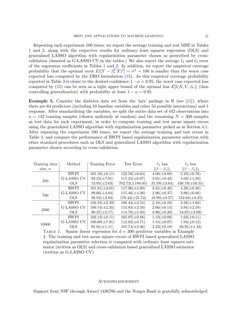
RWPI AND APPLICATIONS TO MACHINE LEARNING 41
Repeating each experiment 100 times, we report the average training and test MSE in Tables1 and 2, along with the respective results for ordinary least squares regression (OLS) andgeneralized LASSO algorithm with regularization parameter chosen as prescribed by cross-validation (denoted as G-LASSO CV in the tables.) We also report the average `1 and `2 errorof the regression coefficients in Tables 1 and 2. In addition, we report the empirical coverageprobability that the optimal error E[(Y − βT∗ X)2] = σ2 = 100 is smaller than the worst caseexpected loss computed by the DRO formulation (15). As this empirical coverage probabilityreported in Table 3 is closer to the desired confidence 1−α = 0.95, the worst case expected losscomputed by (15) can be seen as a tight upper bound of the optimal loss E[l(X,Y ;β∗)] (thuscontrolling generalization) with probability at least 1− α = 0.95.
Example 5. Consider the diabetes data set from the ‘lars’ package in R (see [11]), wherethere are 64 predictors (including 10 baseline variables and other 54 possible interactions) and 1response. After standardizing the variables, we split the entire data set of 442 observations inton = 142 training samples (chosen uniformly at random) and the remaining N = 300 samplesas test data for each experiment, in order to compute training and test mean square errorsusing the generalized LASSO algorithm with regularization parameter picked as in Section 4.1.After repeating the experiment 100 times, we report the average training and test errors inTable 4, and compare the performance of RWPI based regularization parameter selection withother standard procedures such as OLS and generalized LASSO algorithm with regularizationparameter chosen according to cross-validation.
Training data Method Training Error Test Error `1 loss `2 losssize, n ‖β − β∗‖1 ‖β − β∗‖2
350
RWPI 101.16(±8.11) 122.59(±6.64) 4.08(±0.69) 5.23(±0.76)G-LASSO CV 92.23(±7.91) 117.25(±6.07) 3.91(±0.42) 5.02(±1.28)
OLS 13.95(±2.63) 702.73(±188.05) 31.59(±3.64) 436.19(±50.55)
700
RWPI 101.81(±3.01) 117.96(±4.80) 3.31(±0.40) 4.38(±0.48)G-LASSO CV 99.66(±4.64) 115.46(±4.36) 2.96(±0.37) 3.98(±0.66)
OLS 56.82(±3.94) 178.44(±21.74) 10.99(±0.57) 152.04(±8.25)
3500
RWPI 102.55(±2.39) 108.44(±2.54) 2.18(±0.16) 3.28(±1.66)G-LASSO CV 100.74(±2.35) 113.83(±2.33) 2.66(±0.14) 3.91(±2.18)
OLS 90.37(±2.17) 114.78(±5.50) 3.96(±0.20) 54.67(±3.09)
10000
RWPI 102.12(±8.11) 105.97(±0.88) 1.13(±0.08) 1.63(±0.11)G-LASSO CV 100.69(±7.91) 112.82(±0.71) 1.15(±0.07) 1.94(±0.12)
OLS 95.91(±1.11) 107.74(±2.96) 2.23(±0.10) 30.91(±1.43)Table 1. Sparse linear regression for d = 300 predictor variables in Example4. The training and test mean square errors of RWPI based generalized LASSOregularization parameter selection is compared with ordinary least squares esti-mator (written as OLS) and cross-validation based generalized LASSO estimator(written as G-LASSO CV)
Acknowledgement
Support from NSF through Award 1436700 and the Norges Bank is gratefully acknowledged.

42 BLANCHET, KANG AND MURTHY
Training data Method Training Error Test Error `1 loss `2 losssize, n ‖β − β∗‖1 ‖β − β∗‖2
350
RWPI 108.05(±8.38) 109.46(±4.68) 4.02(±0.71) 4.08(±0.70)G-LASSO CV 93.17(±10.83) 104.51(±4.76) 2.23(±0.38) 6.89(±2.35)
OLS − − − −
700
RWPI 104.33(±5.03) 103.18(±2.14) 2.91(±0.42) 2.99(±0.43)G-LASSO CV 100.50(±4.70) 99.92(±2.18) 1.45(±0.28) 2.82(±0.64)
OLS 14.27(±2.02) 699.06(±137.45) 31.66(±2.21) 518.02(±44.87)
3500
RWPI 101.52(±2.52) 96.38(±0.80) 1.23(±0.24) 1.32(±0.24)G-LASSO CV 102.58(±2.49) 98.55(±0.94) 1.18(±0.15) 1.94(±0.24)
OLS 82.22(±2.31) 102.01(±6.14) 6.76(±0.23) 114.05(±5.73)
10000
RWPI 101.36(±1.11) 94.86(±0.36) 0.75(±0.13) 0.81(±0.14)G-LASSO CV 103.00(±1.11) 98.55(±0.49) 1.16(±0.08) 1.94(±0.13)
OLS 95.11(±1.10) 99.53(±4.83) 3.26(±0.11) 63.67(±2.16)Table 2. Sparse linear regression for d = 600 predictor variables in Example4. The training and test mean square errors of RWPI based generalized LASSOregularization parameter selection is compared with ordinary least squares esti-mator (written as OLS) and cross-validation based generalized LASSO estimator(written as G-LASSO CV). As n < d when n = 350, OLS estimation is not ap-plicable in that case (denoted by a blank)
No. of predictors Training sample sized 350 700 3500 10000
300 0.974 0.977 0.975 0.969600 0.963 0.966 0.970 0.968
Table 3. Coverage Probability of empirical worst case expected loss in Example 4
Training Error Testing ErrorRWPI 0.58(±0.05) 0.60(±0.04)
G-LASSO CV 0.44(±0.06) 0.57(±0.03)OLS 0.26(±0.05) 1.38(±0.68)
Table 4. Linear Regression for Diabetes data in Example 5 with 142 trainingsamples and 300 test samples. The training and test mean square errors of RWPIbased generalized LASSO regularization parameter selection is compared withordinary least squares estimator (written as OLS) and cross-validation basedgeneralized LASSO estimator (written as G-LASSO CV).
References
[1] Pierre Alquier. LASSO, iterative feature selection and the correlation selector: Oracle inequalities andnumerical performances. Electronic Journal of Statistics, 2:1129–1152, 2008.
[2] Arindam Banerjee, Sheng Chen, Farideh Fazayeli, and Vidyashankar Sivakumar. Estimation with normregularization. In Advances in Neural Information Processing Systems 27, pages 1556–1564. 2014.
[3] Alexandre Belloni, Victor Chernozhukov, and Lie Wang. Square-root LASSO: pivotal recovery of sparsesignals via conic programming. Biometrika, 98(4):791–806, 2011.
[4] Patrick Billingsley. Convergence of probability measures. John Wiley & Sons, 2013.[5] Jose Blanchet and Yang Kang. Sample-out-of-sample inference based on Wasserstein distance. arXiv preprint
arXiv: 1605.01340, 2016.

RWPI AND APPLICATIONS TO MACHINE LEARNING 43
[6] Jose Blanchet and Karthyek Murthy. Quantifying distributional model risk via optimal transport. arXivpreprint arXiv:1604.01446, 2016.
[7] Francesco Bravo. Empirical likelihood based inference with applications to some econometric models. Econo-metric Theory, 20(02):231–264, 2004.
[8] Emmanuel Candes and Terence Tao. The Dantzig selector: Statistical estimation when p is much larger thann. Ann. Statist., 35(6):2313–2351, 12 2007.
[9] Song Xi Chen and Peter Hall. Smoothed empirical likelihood confidence intervals for quantiles. The Annalsof Statistics, 21(3):1166–1181, September 1993.
[10] Victor Chernozhukov, Denis Chetverikov, and Kengo Kato. Gaussian approximations and multiplier boot-strap for maxima of sums of high-dimensional random vectors. Ann. Statist., 41(6):2786–2819, 12 2013.
[11] Bradley Efron, Trevor Hastie, Iain Johnstone, and Robert Tibshirani. Least angle regression. The Annals ofstatistics, 32(2):407–499, 2004.
[12] Peyman Esfahani and Daniel Kuhn. Data-driven distributionally robust optimization using the Wassersteinmetric: Performance guarantees and tractable reformulations. arXiv preprint arXiv:1505.05116, 2015.
[13] Nicolas Fournier and Arnaud Guillin. On the rate of convergence in Wasserstein distance of the empiricalmeasure. Probability Theory and Related Fields, 162(3-4):707–738, 2015.
[14] Charlie Frogner, Chiyuan Zhang, Hossein Mobahi, Mauricio Araya, and Tomaso A Poggio. Learning with aWasserstein loss. In Advances in Neural Information Processing Systems 28, pages 2053–2061. 2015.
[15] Rui Gao and Anton J. Kleywegt. Distributionally robust stochastic optimization with Wasserstein distance.arXiv preprint arXiv:1604.02199v1, 2016.
[16] Trevor Hastie, Robert Tibshirani, Jerome Friedman, and James Franklin. The elements of statistical learning:data mining, inference and prediction. The Mathematical Intelligencer, 27(2):83–85, 2005.
[17] Nils Lid Hjort, Ian McKeague, and Ingrid Van Keilegom. Extending the scope of empirical likelihood. TheAnnals of Statistics, pages 1079–1111, 2009.
[18] Keiiti Isii. On sharpness of Tchebycheff-type inequalities. Annals of the Institute of Statistical Mathematics,14(1):185–197, 1962.
[19] Xingguo Li, Tuo Zhao, Xiaoming Yuan, and Han Liu. The flare package for high dimensional linear regressionand precision matrix estimation in R. The Journal of Machine Learning Research, 16(1):553–557, 2015.
[20] Sahand Negahban, Pradeep Ravikumar, Martin Wainwright, and Bin Yu. A unified framework for high-dimensional analysis of M-Estimators with decomposable regularizers. Statistical Science, 27(4):538–557,2012.
[21] Whitney Newey and Richard Smith. Higher order properties of GMM and generalized empirical likelihoodestimators. Econometrica, 72(1):219–255, 2004.
[22] XuanLong Nguyen. Convergence of latent mixing measures in finite and infinite mixture models. The Annalsof Statistics, 41(1):370–400, 2013.
[23] Art Owen. Empirical likelihood ratio confidence intervals for a single functional. Biometrika, 75(2):237–249,1988.
[24] Art Owen. Empirical likelihood ratio confidence regions. The Annals of Statistics, pages 90–120, 1990.[25] Art Owen. Empirical likelihood for linear models. The Annals of Statistics, pages 1725–1747, 1991.[26] Art Owen. Empirical likelihood. CRC press, 2001.[27] Samet Oymak, Christos Thrampoulidis, and Babak Hassibi. The squared-error of generalized LASSO: A
precise analysis. In In proceedings of the 51st Annual Allerton Conference of Communication, Control, andComputing, pages 1002–1009, October 2013.
[28] Gabriel Peyre, Marco Cuturi, and Justin Solomon. Gromov-Wasserstein averaging of kernel and distancematrices. In ICML, 2016.
[29] Jin Qin and Jerry Lawless. Empirical likelihood and general estimating equations. The Annals of Statistics,pages 300–325, 1994.
[30] Svetlozar T Rachev and Ludger Ruschendorf. Mass Transportation Problems. Volume I: Theory. SpringerScience & Business Media, 1998.
[31] Svetlozar T Rachev and Ludger Ruschendorf. Mass Transportation Problems. Volume II: Applications.Springer Science & Business Media, 1998.
[32] Antoine Rolet, Marco Cuturi, and Gabriel Peyre. Fast dictionary learning with a smoothed Wasserstein loss.In Proceedings of the 19th International Conference on Artificial Intelligence and Statistics, pages 630–638,2016.
[33] Yossi Rubner, Carlo Tomasi, and Leonidas J. Guibas. The earth mover’s distance as a metric for imageretrieval. International Journal of Computer Vision, 40(2):99–121, 2000.

44 BLANCHET, KANG AND MURTHY
[34] Vivien Seguy and Marco Cuturi. Principal geodesic analysis for probability measures under the optimaltransport metric. In Advances in Neural Information Processing Systems 28, pages 3312–3320. 2015.
[35] Soroosh Shafieezadeh-Abadeh, Peyman Esfahani, and Daniel Kuhn. Distributionally robust logistic regres-sion. In Advances in Neural Information Processing Systems 28, pages 1576–1584. 2015.
[36] James Smith. Generalized Chebychev inequalities: Theory and applications in decision analysis. OperationsResearch, 43(5):807–825, 1995.
[37] Justin Solomon, Fernando de Goes, Gabriel Peyre, Marco Cuturi, Adrian Butscher, Andy Nguyen, Tao Du,and Leonidas Guibas. Convolutional Wasserstein distances: Efficient optimal transportation on geometricdomains. ACM Trans. Graph., 34(4):66:1–66:11, July 2015.
[38] Justin Solomon, Raif Rustamov, Leonidas Guibas, and Adrian Butscher. Earth mover’s distances on discretesurfaces. ACM Trans. Graph., 33(4):67:1–67:12, July 2014.
[39] Sanvesh Srivastava, Volkan Cevher, Quoc Tran-Dinh, and David B Dunson. Wasp: Scalable bayes viabarycenters of subset posteriors. In AISTATS, 2015.
[40] Frode Terkelsen. Some minimax theorems. Mathematica Scandinavica, 31(2):405–413, 1973.[41] Robert Tibshirani. Regression shrinkage and selection via the lasso. Journal of the Royal Statistical Society.
Series B (Methodological), pages 267–288, 1996.[42] Cedric Villani. Optimal transport: old and new. Springer Science & Business Media, 2008.[43] Changbao Wu. Weighted empirical likelihood inference. Statistics & Probability Letters, 66(1):67–79, January
2004.[44] Huan Xu, Constantine Caramanis, and Shie Mannor. Robust regression and LASSO. In Advances in Neural
Information Processing Systems 21, pages 1801–1808. 2009.[45] Huan Xu, Constantine Caramanis, and Shie Mannor. Robustness and regularization of support vector ma-
chines. J. Mach. Learn. Res., 10:1485–1510, December 2009.[46] Mai Zhou. Empirical likelihood method in survival analysis, volume 79. CRC Press, 2015.
Appendix
Appendix A. Strong duality of the linear semi-infinite programs in the paper
In the main body of the paper, we have utilized strong duality of linear semi-infinite programsin two contexts: 1) to derive a dual representation of the RWP function in order to performasymptotic analysis (see Proposition 1), and 2) to derive distributional robust representations(see Proposition 4). Establishing these strong dualities rely on the following well-known resulton problem of moments ([18, 21]).
The problem of moments. Let Ω be a nonempty Borel measurable subset of Rm, which, inturn, is endowed with the Borel sigma algebra BΩ. Let X be a random vector taking values inthe set Ω, and f = (f1, . . . , fk) : Ω → Rk be a vector of moment functionals. Let PΩ and M+
Ωdenote, respectively, the set of probability and non-negative measures, respectively on (Ω,BΩ)such that the Borel measurable functionals φ, f1, f2, . . . , fk, defined on Ω, are all integrable.Given a real vector q = (q1, . . . , qk), the objective of the problem of moments is to find theworst-case bound,
v(q) := supEµ[φ(X)] : Eµ[f(X)] = q, µ ∈ PΩ
.(49)
If we let f0 = 1Ω, it is convenient to add the constraint, Eµ[f0(X)] = 1, by appending
f = (f0, f1, . . . , fk), q = (1, q1, . . . , qk), and consider the following reformulation of the aboveproblem:
v(q) := sup
∫φ(x)dµ(x) :
∫f(x)dµ(x) = q, µ ∈M+
Ω
.(50)
Then, under the assumption that a certain Slater’s type of condition is satisfied, one has thefollowing equivalent dual representation for the moment problem (50). See Theorem 1 (and thediscussion of Case [I] following Theorem 1) in [18] for a proof of the following result:

RWPI AND APPLICATIONS TO MACHINE LEARNING 45
Proposition 6. Let Qf = ∫
f(x)dµ(x) : µ ∈ M+Ω
. If q = (1, q1, . . . , qk) is an interior point
of Qf , then
v(q) = inf
k∑i=0
aiqi : ai ∈ R,k∑i=0
aifi(x) ≥ φ(x) for all x ∈ Ω
.
In the rest of this section, we recast the dual reformulation of RWP function (in (1)) and thedual reformulation of the distributional representation in Proposition 4 as particular cases ofthe dual representation of the problem of moments in Proposition 6.
Dual representation of RWP function Recall from Section 2.3 that W is a random vectortaking values in Rm and h(·, θ) is Borel measurable.
Proof of Proposition 1. For simplicity, we do not write the dependence on parameter θ in h(u, θ)and Rn(θ) in this proof; nevertheless, we should keep in mind that the RWP function is afunction of parameter θ. Given estimating equation E[h(W )] = 0. Recall the definition of thecorresponding RWP function,
Rn := infDc(P, Pn) : EP
[h(W )
]= 0
= inf
Eπ[c(U,W )
]: Eπ
[h(U)
]= 0, πW = Pn, π ∈ P(Rm × Rm)
.
where πW denotes the marginal distribution of W. To recast this as a problem of moments asin (49), let Ω = (u,w) ∈ Rm × Rm : c(u,w) <∞,
f(u,w) =
1w=W1
(u,w)
1w=W2(u,w)
...1w=Wn
(u,w)
h(u)
and q =
1/n1/n
...1/n0
.
Further, let φ(u,w) = −c(u,w), for all (u,w) ∈ Ω. Then,
Rn = − supEπ[φ(U,W )
]: Eπ
[f(U,W )
]= q, π ∈ PΩ
,
is of the same form as (49). Let H denote the convex hull of the range h(u) : (u,w) ∈ Ω.Then, following the definition of Qf in the abstract formulation in Proposition 6, we obtain
Qf = Rn+1+ ×H. As 0 lies in the interior of convex hull H, it is immediate that the Slater’s
condition, q = (1, q) lying in the interior of the Qf , is satisfied. Consequently, we obtain the
following dual representation of Rn due to Proposition 6:
Rn = − infai∈R
a0 +
1
n
n∑i=1
ai : a0 +
n∑i=1
ai1w=Wi(u,w)
+k∑
i=n+1
aihi(u) ≥ −c(u,w), for all (u,w) ∈ Ω
= − infai∈R
a0 +
1
n
n∑i=1
ai : a0 + ai ≥ supu:c(u,Wi)<∞
−c(u,Wi)−
k∑i=n+1
aihi(u)
.

46 BLANCHET, KANG AND MURTHY
As the inner supremum is not affected even if we take supremum over u : c(u,Wi) =∞, afterletting λ = (an+1, . . . , ak) for notational convenience, we obtain
Rn = supλ
1
n
n∑i=1
infu∈Rm
c(u,Wi) + λTh(u)
(51)
As λ is a free variable, we flip the sign of λ to arrive at the statement of Proposition 1. Thiscompletes the proof.
Dual representation of the DRO formulation in (15) Here, we provide a proof for thedual representation in Proposition 4 that has been instrumental in establishing the distributionalrobust representations of LASSO and regularized logistic regression.
Proof of Proposition 4. Given a Borel measurable g, our first objective is to prove that theworst-case loss supEP [g(W )] : Dc(P, Pn) ≤ δ admits the dual representation,
supEP [g(W )] : Dc(P, Pn) ≤ δ = infλ≥0
λδ +
1
n
n∑i=1
φλ(Wi)
,(52)
with φλ(Wi) = supug(u) − λc(u,w). This would essentially prove Proposition 4 if we letW = (X,Y ), g(W ) = l(X,Y ;β) and φλ(X,Y ;β) = φλ(W ).
Since the problem supEP [g(W )] : Dc(P, Pn) ≤ δ has inequality constraints, one way is toproceed exactly as in RWP dual formulation above except for restricting the Lagrange multipliercorresponding to the equality constraint to be non-negative. Alternatively, one can recast theproblem as in (49) with the introduction of a slack variable S as below:
supEP [g(W )] : Dc(P, Pn) ≤ δ
= sup
Eπ[g(U)
]: Eπ
[c(U,W ) + S
]= δ, πW = Pn, π(S = v) = 1, π ∈ P(Rm × Rm × R+)
.
In the context of notation introduced for the problem of moments described at the beginningof this appendix, let Ω = (u,w, s) : c(u,w) <∞, s ≥ 0,
f(u,w, s) =
1w=W1(u,w, s)
1w=W2(u,w, s)...
1w=Wn(u,w, s)
1s=vc(u,w) + s
and q =
1/n1/n
...1/n1δ
.
In addition, if we let φ(u,w, s) = g(u), then
supEP [g(W )] : Dc(P, Pn) ≤ δ
= sup
Eπ[φ(U,W,S)] : Eπ[f(U,W,S)] = q, π ∈ PΩ
,
is a problem of moments of the form (49). Similar to the RWP dual formulation discussed earlierin the section, q = (1, q) lies in the interior of Qf = Rn+3
+ , thus satisfying Slater’s condition for
all δ > 0. Then, due to Proposition 6, we obtain
supEP [g(W )] : Dc(P, Pn) ≤ δ
= inf
a∈A
a0 +
1
n
n∑i=1
ai + an+1 + an+2δ

RWPI AND APPLICATIONS TO MACHINE LEARNING 47
where the set A is the collection of a = (a0, a1, . . . , an+1) ∈ Rn+3 such that
a0 +
n∑i=1
ai1w=Wi(u,w, s) + an+11s=v(u,w, s) + an+2
(c(u,w) + s
)≥ g(u),
for all (u,w, s) ∈ Ω. Further, observe that the value of the optimization problem above does notchange, even if we consider only the following constraints:
a0 + ai + an+1 ≥ sup
g(u)− an+2
(c(u,Wi) + s
): u ∈ Rm, s ≥ 0
=
supu∈Rm
g(u)− an+2c(u,Wi)
if an+2 ≥ 0,
∞ if an+2 < 0.
If we recall the notation that φλ(Wi) = supu∈Rm g(u)− λc(u,Wi) , then
supEP [g(W )] : Dc(P, Pn) ≤ δ
= inf
an+2≥0ai∈R,
a0 +
1
n
n∑i=1
ai + an+1 + an+2δ : a0 + ai + an+1 ≥ φan+2(Wi)
= inf
an+2≥0
φan+2(Wi) + an+2δ
,
thus proving (52). As explained earlier, letting W = (X,Y ), g(W ) = l(X,Y ;β) and φλ(X,Y ;β)in (52) verifies the proof of Proposition 4.
Appendix B. Exchange of sup and inf in the DRO formulation (15)
Proposition 7. Let us write
Uδ =P : Dc
(P, Pn
)≤ δ,
and define
g (β) = supP∈Uδ
EP[l(X,Y ;β
)].
Suppose that g (·) is convex and assume that there exists b ∈ R such that κb = β : g (β) ≤ bis compact and non-empty. In addition, suppose that EP
[l(X,Y ;β
)]is lower semi-continuous
and convex as a function of β throughout κb. Then,
minβ∈Rd
supP :Dc
(P,Pn
)≤δEP[l(X,Y ;β
)]= sup
P :Dc(P,Pn
)≤δ
minβ∈Rd
EP[l(X,Y ;β
)].
Proof. By definition of κb we have that
minβ∈Rd
supP :Dc
(P,Pn
)≤δEP[l(X,Y ;β
)]= min
β∈κbsup
P :Dc(P,Pn
)≤δEP[l(X,Y ;β
)].
By a min-max result of Terkelsen (see Corollary 2 in [40]), since both Uδ and κb are convex, κbis compact, EP
[l(X,Y ;β
)]is lower semi-continuous and convex throughout κb as a function of
β, and EP[l(X,Y ;β
)]is concave as a function of P , then
minβ∈κb
supP :Dc
(P,Pn
)≤δEP[l(X,Y ;β
)]= sup
P :Dc(P,Pn
)≤δ
minβ∈κb
EP[l(X,Y ;β
)].

48 BLANCHET, KANG AND MURTHY
The proof is complete if are able to argue the identity
supP :Dc
(P,Pn
)≤δ
minβ∈κb
EP[l(X,Y ;β
)]= sup
P :Dc(P,Pn
)≤δ
minβ∈Rd
EP[l(X,Y ;β
)].
To see this, note that we always have
supP :Dc
(P,Pn
)≤δ
minβ∈κb
EP[l(X,Y ;β
)]≥ sup
P :Dc(P,Pn
)≤δ
minβ∈Rd
EP[l(X,Y ;β
)].(53)
Let us assume that the strict inequality holds. If this is the case then we most have that thereexists β′ /∈ κb such that
b < g(β′)
= supP :Dc
(P,Pn
)≤δEP[l(X,Y ;β′
)]< sup
P :Dc(P,Pn
)≤δ
minβ∈κb
EP[l(X,Y ;β
)]≤ b
where the second inequality follows because we are assuming that (53) holds with strict inequal-ity, and the last inequality follows because for each β ∈ κb
minβ∈κb
EP[l(X,Y ;β
)]≤ EP
[l(X,Y ;β
)].
We therefore contradict the assumption that the strict inequality in (53) holds. Hence, theproof is complete.
Proof of Lemma 1. Let us consider linear regression loss function first. Under null hypothesis,E‖X‖22 <∞ and E[e2] <∞. Therefore, for any β ∈ Rd, E[l(X,Y ;β)] = E[(Y − βTX)2] <∞.Further, as the loss function l(x, y;β) is a convex function of β,
g(β) = supP∈ Uδ
EP [l(X,Y ;β)] =
(√EPn [(Y − βTX)2] +
√δ‖β‖p
)2
is convex as well and finite for all β in Rd (the second equality follows from the distributionalrobust representation in Theorem 2). Further, as g(β) → ∞ when ‖β‖p → ∞ and g(β) is
convex and continuous in Rd, the level sets κb = β : g(β) ≤ b are compact and nonempty
as long as b > (√EPn [(Y − βT∗ X)2] +
√δ‖β∗‖)2. Finally, due to the convexity and finiteness of
E[l(X,Y ;β)] lower semi-continuity of E[l(X,Y ;β)] is immediate as well. As all the conditionsin Proposition 7 are satisfied, the sup and inf in the DRO formulation (15) can be exchangedin the linear regression example as a consequence of Proposition 7.
It is straightforward to check that exactly same argument applies for logistic regression lossfunction as well when E‖X‖22 is finite.
E-mail address: [email protected], [email protected], [email protected]