johnson et al 2014 plasticidad fenotipica mortandad selectiva peces variacion

REV IEW AND

SYNTHES IS Phenotypic variation and selective mortality as major drivers

of recruitment variability in fishes

Darren W. Johnson,1* Kirsten

Grorud-Colvert,2 Su Sponaugle3,2

and Brice X. Semmens1

1Marine Biology Research Division,

Scripps Institution of Oceanogra-

phy, UC San Diego, La Jolla, CA,

92023, USA2Department of Integrative Biology,

Oregon State University, 3029

Cordley Hall, Corvallis, Oregon,

97330, USA3Marine Biology and Fisheries,

Rosenstiel School of Marine and

Atmospheric Science, University of

Miami, 4600 Rickenbacker Cause-

way, Miami, Florida, 33149, USA

*Correspondence and present

address: Department of Biological

Sciences, California State University,

Long Beach. 1250 Bellflower Blvd.,

Long Beach, CA, 90840, USA.

E-mail: [email protected]

Abstract

An individual’s phenotype will usually influence its probability of survival. However, when evalu-ating the dynamics of populations, the role of selective mortality is not always clear. Not all mor-tality is selective, patterns of selective mortality may vary, and it is often unknown how selectivemortality compares or interacts with other sources of mortality. As a result, there is seldom aclear expectation for how changes in the phenotypic composition of populations will translate intodifferences in average survival. We address these issues by evaluating how selective mortalityaffects recruitment of fish populations. First, we provide a quantitative review of selective mortal-ity. Our results show that most of the mortality during early life is selective, and that variation inphenotypes can have large effects on survival. Next, we describe an analytical framework thataccounts for variation in selection, while also describing the amount of selective mortality experi-enced by different cohorts recruiting to a single population. This framework is based on recon-structing fitness surfaces from phenotypic selection measurements, and can be employed for eithersingle or multiple traits. Finally, we show how this framework can be integrated with models ofdensity-dependent survival to improve our understanding of recruitment variability and popula-tion dynamics.

Keywords

Density-dependent selection, fitness surface, natural selection, population dynamics, stock–recruitrelationships.

Ecology Letters (2014) 17: 743–755

INTRODUCTION

The dynamics of populations can be affected by both thequantity and quality of the individuals within them. That is,the demographic processes that drive the dynamics of popula-tions are influenced by both the number of individuals andthe phenotypes of those individuals. Classic theory has em-phasised numerical effects such as density-dependent regula-tion as the major, endogenous force driving the dynamics ofpopulations (reviewed by Murdoch 1994; Cappuccino & Price1995). However, the phenotypic composition of a populationcan also exert a strong influence on population dynamics,especially if the phenotypes under study are closely related todemographic components of fitness (reviewed by Gaillardet al. 2000; Hairston et al. 2005; Schoener 2011). Despitethese observations, in practice it can be difficult to predicthow changes in the distribution of phenotypes within a popu-lation will actually translate into variation in populationdynamics (reviewed by Saccheri & Hanski 2006; Kokko &L�opez-Sepulcre 2007; Metcalf & Pavard 2007). This is particu-larly true for processes such as population replenishment,which may depend on complex, non-linear relationshipsamong phenotype, mortality and density.Although it has long been recognised that the phenotypic

composition of populations will influence their dynamics, anoverall appreciation of the magnitude of these effects (espe-cially relative to environmental factors as a source of variabil-

ity) has advanced more slowly (reviewed by Thompson 1998;Benton et al. 2006; Kokko & L�opez-Sepulcre 2007; Pelletieret al. 2009). In part, this delay has been because classicaldemographic analyses and models (in which individuals aretreated as identical) are simple and accessible, whereas thequantitative tools for analysing phenotypic variation (and itsrelative influence on dynamics) require more data and havetaken time to develop (e.g. Lande 1976; Lande & Arnold1983; Bjørnstad & Hansen 1994; Van Tienderen 2000;Smallegange & Coulson 2013). A major advance in this fieldcame when Hairston et al. (2005) presented a general frame-work for disentangling the influences of both phenotypic traitchange and environmental variation on population dynamics(also see Ellner et al. 2011 for extensions of this approach). Inthis framework, the partitioning of environmental and pheno-typic contributions to population dynamics is accomplishedby analysing time-series observations of population-levelresponses (e.g. population size), and average values of bothphenotypes and environmental variables of interest. Thisframework has been applied to several empirical studies (e.g.Ezard et al. 2009; also see examples in Hairston et al. 2005;Ellner et al. 2011), and can be quite successful at illustratinghow phenotype change can affect dynamics. However, astrong (and potentially limiting) assumption of the methodsproposed by Hairston and colleagues is that any effects ofchanges in the distribution of phenotypes are a function ofchanges in the mean value. This assumption may hold if the

© 2014 John Wiley & Sons Ltd/CNRS

Ecology Letters, (2014) 17: 743–755 doi: 10.1111/ele.12273

relationships between phenotypes and population responsevariables (e.g. per capita growth rate, survival, fecundity, etc.)are linear (Ellner et al. 2011). However, if such relationshipsare not linear, then through non-linear averaging (e.g. Ruel &Ayres 1999) both the means and variances of phenotype dis-tributions can play an important role in population dynamics,and other approaches are needed. In this study, we present aframework that can accommodate strong non-linearities in therelationships between phenotypes and fitness and thus can bevery useful in analysing how phenotypic variation can affectpopulation dynamics, even in the presence of strong densitydependence (another non-linear relationship). We apply thisframework to studies of selective mortality in fish populationsand use it to shed light on how variation in phenotypes maydrive variability in recruitment.Replenishment of fish populations is notoriously variable.

In part, this is because most fishes have life histories in whichnumerous offspring are produced, but very few survive toadulthood. A consequence of having a life history in whichearly stages can be extremely abundant (often outnumberingadults by several orders of magnitude) is that even smallchanges in mortality during early life can have large effects onrecruitment (Houde 1987). Because seemingly small variationsin mortality easily can be responsible for order-of-magnitudefluctuations in recruitment, scientists have long been interestedin the characteristics of individuals that drive variation inmortality during early life (e.g. Anderson 1988; Miller et al.1988, Bailey & Houde 1989; Houde 2008).The relationship between individual phenotype and relative

survival during early life can be examined through the lens ofphenotypic selection analysis (Lande & Arnold 1983). Pheno-typic selection analysis has long been used to understand evo-lutionary trajectories, but a main feature is that it separatesselection from inheritance. When such analyses are madewithout information on heredity, they cannot be used to pre-dict evolution. However, they may still be used to understandselection as a within-generation, demographic process.The last few decades have seen a rise of studies examining

how the relative survival of fishes is influenced by phenotypiccharacteristics. The realisation that fish otoliths (accretions ofcalcium carbonate around protein matrices in the inner ear)can carry a permanent record of traits related to size, growthrate, and condition has enabled studies of selective mortalityand yielded important insight into why certain individuals sur-vive and others do not (Sponaugle 2010). Recent reviews ofthis field indicate that selection (i.e. the change in the pheno-type distribution that is generated by differential mortality) istypically very strong during early life phases of fishes (Sogard1997; Perez & Munch 2010). Both of these reviews noted asubstantial amount of variability in selection, although neitherstudy examined selective mortality at the scale of the popula-tion, and neither study explored how variation in selectionmay affect population dynamics. Selection during early lifecan be summarised using selection coefficients, but it is impor-tant to keep in mind that survival during early life is only acomponent of fitness. From an evolutionary viewpoint, onemight expect early mortality to be strongly selective withrespect to traits such as size and growth (which are commonlymeasured traits in this field). Mothers may trade offspring size

for offspring number, and the maximisation of fitness maycome at the expense of offspring survival (Vance 1973; Smith& Fretwell 1974). As a result, the relationship between earlylife traits and a more complete measure of fitness (e.g. lifetimereproductive success of mothers) may indicate stabilising,rather than directional, selection because reproductive successis a combination of both the number of offspring and theirsurvival (e.g. Smith & Fretwell 1974; see Einum & Fleming2000; Johnson et al. 2010; for empirical examples in fishes).A consequence of this phenomenon is that even though earlylife-history traits may be evolutionarily stable, there can stillbe very large differences in the relative probability of survivalof individuals during early life (as evidenced by many empiri-cal studies; Sogard 1997; Perez & Munch 2010).That selection is widespread and often strong provides evi-

dence that an individual’s phenotype can strongly influence itsrelative probability of survival. However, at the level of thepopulation, understanding how phenotypic variability affectsrecruitment is much more complicated. First, it can be unclearwhether the amount of selective mortality incurred is substan-tial enough to be important to the dynamics of populations.The amount of selective mortality that a population or acohort (i.e. a group of similarly aged individuals) experiences,and how that compares to total mortality, is not often quanti-fied. Second, selection may be highly variable. Even when oneconsiders selection on a single trait in a focal population,measurements often vary substantially (e.g. Meekan & Fortier1996; Good et al. 2001; Rankin & Sponaugle 2011), making itdifficult to discern any general patterns. Finally, it remainsunclear how selective mortality compares or interacts withdensity-dependent mortality – a major factor influencing earlysurvival and recruitment (reviewed by Myers & Cadigan 1993;Rose et al. 2001; Hixon & Webster 2002). Box 1 outlines ageneral approach to quantifying selective mortality and topartitioning population-level mortality into selective and non-selective components.To understand how phenotypic variation affects mortality

within cohorts and therefore recruitment to populations, weneed to study selection within a quantitative, analytical frame-work. Here, we review empirical studies of selection in fishesas a first step towards evaluating the overall importance ofselective mortality to recruitment. Next, we describe an ana-lytical framework that accounts for variation in selection,while also describing the amount of selective mortality experi-enced by cohorts. This framework is based on empiricalreconstruction of fitness surfaces from selection measure-ments, and can be employed for either single, or multipletraits. Finally, we show how this framework can be integratedwith models of density-dependent survival to improve ourunderstanding of recruitment variability.

SELECTION, DEMOGRAPHIC COSTS AND

RECRUITMENT VARIABILITY IN FISHES

Selection implies a demographic cost to the population. Whenphenotype distributions change through differential mortality,stronger selection implies greater mortality overall. Demo-graphic costs of selection can therefore be important in thecontext of recruitment where dynamics are driven by variation


744 D. W. Johnson et al. Review and Synthesis

in both cohort size and cohort mortality. All else being equal,cohorts that experience stronger selection must incur greatermortality (i.e. greater costs), and if cohorts that recruit to apopulation vary in the degree of selection (and selective mor-tality), then selective mortality may be an important source ofvariability in total mortality, and thus variability in recruit-ment (Box 1).As a first step towards evaluating variability in selective

mortality and its potential role in generating recruitment vari-ability, we compiled published estimates of selection on earlylife traits in fishes. For many fishes, synchrony in reproductionand/or settlement from the plankton produces discrete cohortsthat settle at approximately the same age. Selection measure-ments are typically made within cohorts and selection measure-ments can be used to infer mortality (Box 1). To evaluate howselective mortality affects recruitment to particular popula-tions, we need to examine variability in selective mortalityamong cohorts because it is among-cohort variation in mortal-ity that contributes to recruitment variability. In our literaturesearch, we considered only those studies that estimated selec-tion on the same focal trait(s) for two or more separatecohorts. Our search yielded a total of 136 selection estimatesfor 33 species (Table S1, also see Appendix S1 in Supporting

Information). Although very few studies of selection haveactual estimates of total mortality, we were able to derive esti-mates of selective mortality from measurements of selection.Selection is typically measured by the selection differential,

i.e. the mean phenotypic value of the population after selectionminus the mean before selection (Falconer & Mackay 1996).For each cohort, we estimated the amount of selective mortalitythat would be necessary to generate the observed selection dif-ferential, given the assumption that before selection, traits werenormally distributed with the observed means and variances.For this analysis, selection was assumed to be generated bytruncation mortality (e.g. all individuals with phenotypic valuesabove a certain threshold (zt) survived and all below died – thispattern could be reversed if smaller phenotypes were favoured).For example, fz = 0 for z > zt and fz = ∞ for z ≤ zt. To calculatetruncation mortality, we used a simple optimisation routine tofind the truncation point on a standard normal distribution thatwould produce a truncated distribution of ‘survivors’ with amean value that would produce the same standardised selectiondifferential as the one observed for each cohort. We then calcu-lated selective mortality as 1 minus the integral of the truncateddistribution. We chose truncation as the functional form ofselection because it is the most efficient form of selection, and

Box 1 Components of mortality

Consider a population in which individuals risk mortality from multiple sources, some of which are selective with respect tophenotype, and others that are not. Let nz,t describe the number of individuals of phenotype z at time t. This distribution willchange through time as individuals are removed from the population through both selective and non-selective mortality. Therate of selective mortality, fz, is a function of phenotype and the rate of non-selective mortality, a, is a constant. There-fore,

@nz;t@t ¼ �anz;t � fznz;t:

From the previous expression, the distribution of phenotypes at time t + 1 can be obtained: nz;tþ1 ¼ nz;te�a�fz

and population size (total abundance) at time t + 1 is then Ntþ1 ¼Rnz;tþ1 dz ¼ e�a

Re�fznz;tdz:

Factoring in the distribution of phenotypes at time t yields Ntþ1 ¼ e�a

Re�fz nz;tdzRnz;tdz

Rnz;tdz;

which can be expressed as: Ntþ1 ¼ e�a

Re�fz nz;tdz

Nt

RNt;

or equivalently Ntþ1 ¼ e�aWzNt;

where Wz ¼ selective survival ¼R

e�fz nz;tdz

Nt:

At the level of the population (or cohort, or group), mortality can be separated into two components: selective mortality (1-Wz), and non-selective mortality Wzð1� e�aÞ.Total mortality (MTOT) is 1 � e�a Wz and may range from 0 to 1. From theserelationships we can conclude that when the selective component of mortality is large, the non-selective component must besmall. We can also conclude that because selective mortality is a component of total mortality, variation in selective mortalityamong cohorts will translate to variation in the total amount of mortality that cohorts experience. This translation will be directif the rate of non-selective mortality (a) is constant among cohorts (or at least random with respect to selective mortality).

In many cases, patterns of selection (i.e. changes in the distributions of phenotypic values) are driven by selective mortality.Even if mortality is not measured directly, the amount of selective mortality a population experiences can be inferred fromselection measurements. Empirical measurements of selection often focus on calculating the selection differential, i.e. the meanphenotypic value after selection minus the mean before selection (Falconer & Mackay 1996). The selection differential (S) canalso be expressed in terms of the (normalised) distribution of phenotypes before selection and the selective mortality function.

Specifically,S ¼R

znz;te�fz dzR

nz;te�fz dz� �z:

If the selection differentials and phenotype distributions are known, and if a simple functional form (e.g. truncation selection)is chosen to describe the rate of selective mortality, then the parameters defining fz can be solved for and the amount of selec-tive mortality can be calculated as described above.


Review and Synthesis Selective mortality and recruitment 745

therefore provides the most conservative estimate of selectivemortality (Van Valen 1965). However, other functional formsof selection are possible. To examine how sensitive the conclu-sions of this analysis would be to choice of functional form, werepeated this analysis assuming that selection can be describedby a less efficient, Gaussian function (Appendix S1). We recog-nise that the functional form of selection may vary amongcohorts, but choosing a single functional form to describe selec-tion allows for a standardised comparison among cohorts, spe-cies, etc. This analysis is therefore meant as a broad-strokesummary of variation in selective mortality.On average, the amount of selective mortality experienced

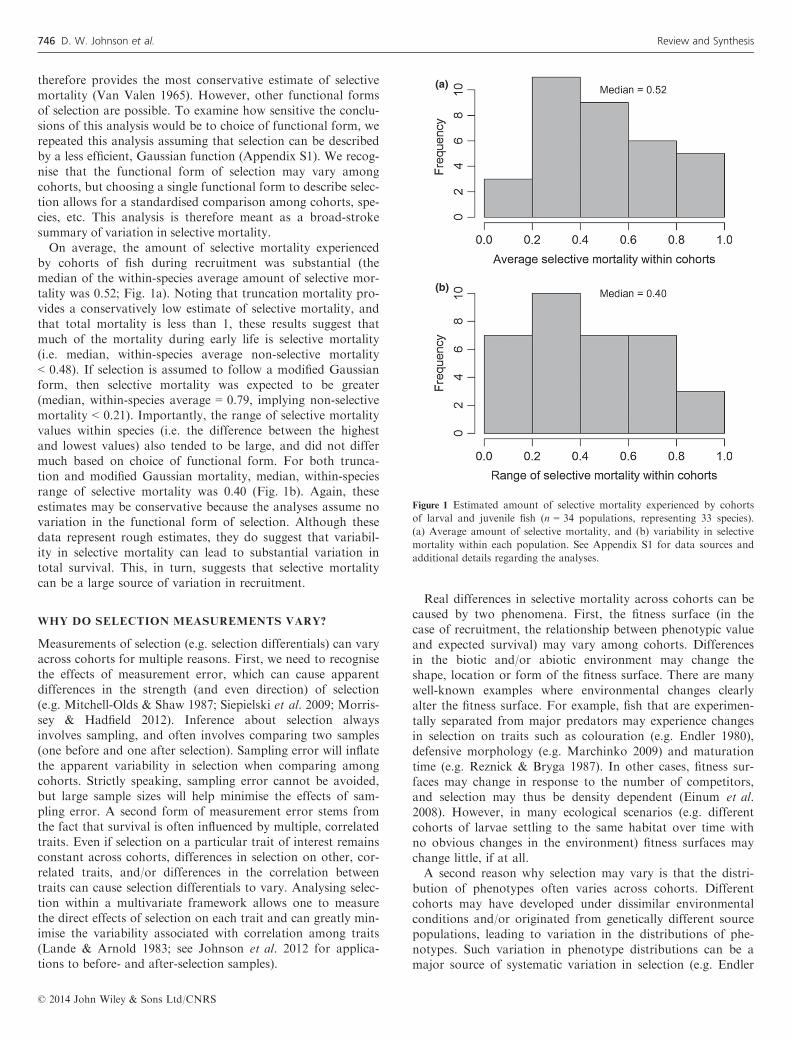
by cohorts of fish during recruitment was substantial (themedian of the within-species average amount of selective mor-tality was 0.52; Fig. 1a). Noting that truncation mortality pro-vides a conservatively low estimate of selective mortality, andthat total mortality is less than 1, these results suggest thatmuch of the mortality during early life is selective mortality(i.e. median, within-species average non-selective mortality< 0.48). If selection is assumed to follow a modified Gaussianform, then selective mortality was expected to be greater(median, within-species average = 0.79, implying non-selectivemortality < 0.21). Importantly, the range of selective mortalityvalues within species (i.e. the difference between the highestand lowest values) also tended to be large, and did not differmuch based on choice of functional form. For both trunca-tion and modified Gaussian mortality, median, within-speciesrange of selective mortality was 0.40 (Fig. 1b). Again, theseestimates may be conservative because the analyses assume novariation in the functional form of selection. Although thesedata represent rough estimates, they do suggest that variabil-ity in selective mortality can lead to substantial variation intotal survival. This, in turn, suggests that selective mortalitycan be a large source of variation in recruitment.

WHY DO SELECTION MEASUREMENTS VARY?

Measurements of selection (e.g. selection differentials) can varyacross cohorts for multiple reasons. First, we need to recognisethe effects of measurement error, which can cause apparentdifferences in the strength (and even direction) of selection(e.g. Mitchell-Olds & Shaw 1987; Siepielski et al. 2009; Morris-sey & Hadfield 2012). Inference about selection alwaysinvolves sampling, and often involves comparing two samples(one before and one after selection). Sampling error will inflatethe apparent variability in selection when comparing amongcohorts. Strictly speaking, sampling error cannot be avoided,but large sample sizes will help minimise the effects of sam-pling error. A second form of measurement error stems fromthe fact that survival is often influenced by multiple, correlatedtraits. Even if selection on a particular trait of interest remainsconstant across cohorts, differences in selection on other, cor-related traits, and/or differences in the correlation betweentraits can cause selection differentials to vary. Analysing selec-tion within a multivariate framework allows one to measurethe direct effects of selection on each trait and can greatly min-imise the variability associated with correlation among traits(Lande & Arnold 1983; see Johnson et al. 2012 for applica-tions to before- and after-selection samples).

Real differences in selective mortality across cohorts can becaused by two phenomena. First, the fitness surface (in thecase of recruitment, the relationship between phenotypic valueand expected survival) may vary among cohorts. Differencesin the biotic and/or abiotic environment may change theshape, location or form of the fitness surface. There are manywell-known examples where environmental changes clearlyalter the fitness surface. For example, fish that are experimen-tally separated from major predators may experience changesin selection on traits such as colouration (e.g. Endler 1980),defensive morphology (e.g. Marchinko 2009) and maturationtime (e.g. Reznick & Bryga 1987). In other cases, fitness sur-faces may change in response to the number of competitors,and selection may thus be density dependent (Einum et al.2008). However, in many ecological scenarios (e.g. differentcohorts of larvae settling to the same habitat over time withno obvious changes in the environment) fitness surfaces maychange little, if at all.A second reason why selection may vary is that the distri-

bution of phenotypes often varies across cohorts. Differentcohorts may have developed under dissimilar environmentalconditions and/or originated from genetically different sourcepopulations, leading to variation in the distributions of phe-notypes. Such variation in phenotype distributions can be amajor source of systematic variation in selection (e.g. Endler

(a)

(b)

Figure 1 Estimated amount of selective mortality experienced by cohorts

of larval and juvenile fish (n = 34 populations, representing 33 species).

(a) Average amount of selective mortality, and (b) variability in selective

mortality within each population. See Appendix S1 for data sources and

additional details regarding the analyses.



1986; Weis et al. 1992; Steele et al. 2011). Central to thisphenomenon is the fact that fitness surfaces are typicallynon-linear. For example, expected survival is boundedbetween 0 and 1, so relationships between phenotype and rel-ative survival can be strongly non-linear. Moreover, it is fre-quently observed that optimal survival often occurs atintermediate, rather than extreme phenotypes (Janzen &Stern 1998). On a non-linear fitness surface that remains con-stant, cohorts with different distributions of phenotypes will‘sample’ different areas of the fitness surface, resulting in dif-ferences in the magnitude, and sometimes even the directionof selection (Fig. 2).Fitness surfaces are not necessarily constant across cohorts,

as changes in the environment may cause fitness surfaces tovary. However, we believe that an essentially constant fitnesssurface is not necessarily a rare scenario. Rigorously evaluat-ing whether fitness surfaces actually differ in space and timerequires multiple estimates of selection and an appropriatenull model for selection variation. When estimates of fitnesssurfaces (or summaries such as selection coefficients) vary, itmay be tempting to conclude that the underlying fitness sur-faces are different. However, we believe that such differencesshould be considered apparent differences in fitness surfacesuntil the effects of sampling different regions of a non-linear,but constant fitness surface can be ruled out.In the sections below, we discuss how a constant fitness sur-

face may provide a parsimonious model to explain variationin selection. When data from multiple cohorts are available,and their distributions of phenotypes vary, systematic varia-tion in selection measurements can provide evidence ofwhether the fitness surface can be treated as constant acrosscohorts. Because cohorts of fish can vary substantially withrespect to the distribution of their phenotypes (in our review,median CV of cohort means = 7.6%, median CV of within-cohort standard deviations = 23.0%), the effects of suchvariation on selective mortality and recruitment may be large.We also discuss how the assumption of a constant fitness sur-face and the techniques described below may be appropriatefor other taxa and ecological scenarios (see Discussion andAppendix S2 in Supporting Information).

RECONSTRUCTING FITNESS SURFACES TO

EVALUATE RECRUITMENT

If fitness surfaces are constant and non-linear, then cohortsthat differ with respect to their distribution of phenotypes willexperience different patterns of selection. However, it is oftenthe case that fitness surfaces are unknown (especially across abroad range of phenotypic values). Rather, investigators typi-cally know the means and variances of trait values before andafter a period of selective mortality, and can thereforeestimate selection. When multiple estimates of selection areavailable, one can look for a systematic relationship betweentrait distributions and selection estimates as evidence of a con-stant fitness surface. If the fitness surface can be assumed tobe reasonably constant, then one can use selection estimatesto reconstruct the fitness surface over a broad range of pheno-typic values. Describing the fitness surface provides a frame-work for inferring differences in selective mortality amongcohorts. This framework can be extremely useful in that it (1)offers an explanation for differences in observed measures ofselection, and (2) describes differences in relative survivalamong cohorts, even when direct measures of mortality areunavailable.To illustrate this approach, we examined variation in selec-

tion on pelagic larval duration (PLD) among cohorts of acommon, demersal blenny (Lipophrys trigloides). Data comefrom Macpherson & Raventos’ (2005) study of post-settle-ment, selective mortality. These authors measured selectivemortality on PLD for eight different cohorts. Samples ofrecent settlers were collected and PLD was measured from ot-oliths. Juveniles of the same cohorts were collected ~45 dayslater. Distributions of PLD values were compared betweeninitial settlers and surviving juveniles in a standard, before-after approach. Note that Macpherson & Raventos (2005)also measured selection on other traits (including size athatching and size at settlement). Here, we concentrate on asingle trait (PLD) to illustrate the analytical approach in theunivariate case. A multivariate approach, which explicitlyconsiders mortality that is selective with respect to multipletraits, is described in a subsequent section.

(a) (b) (c)

Figure 2 Variation in phenotype distributions as a cause of variation in selection measurements. If fitness surfaces are non-linear and constant across cohorts,

then selection differentials, S, will depend on the distributions of phenotypes. (a) When the distribution of phenotypes is centred at the phenotypic optimum

(the peak of the fitness surface), there is no directional selection (S = 0). (b) When phenotypes are, on average, smaller, there is directional selection

favouring larger individuals. (c) When mean phenotype is the same as in (b), but the variance is greater, much more of the phenotype distribution is far out

on the left tail where survival is very low. There is a correspondingly greater shift in the mean, and a greater selection differential. The same principles apply

to the multivariate case, except that selection differentials may also vary because of differences in the distributions of other, correlated traits.



Selection differentials associated with PLD tended to benegative (mean = �1.01, range = �2.37 to 0.46 when standar-dised to a common measure of variance) suggesting thatwithin cohorts, fish that had shorter PLDs tended to survivebetter (shorter PLD is likely related to faster growth and/orbetter condition). Among cohorts, the magnitude of selectionchanged systematically with average phenotypic value(Fig. 3a). Cohorts that had shorter average PLDs experiencedweaker selection, and therefore less selective mortality.Selection differentials describe the slope of the fitness sur-

face at the cohort mean (Phillips & Arnold 1989). If the selec-tion differentials change linearly with mean phenotypic value(and variances are similar among cohorts), it suggests thatover a broad range of phenotypes the fitness surface (i.e. therelationship between phenotypic value and expected fitness)may be reasonably described by a Gaussian function. Definingthe fitness function (Wz) as Gaussian, then

Wz ¼ e�a�ðz�hÞ2zx2 ; ð1Þ

where h is the optimal phenotypic value, x indicates the widthof the curve describing fitness and a specifies the magnitudeof non-selective mortality. A Gaussian fitness function has thedesirable property that fitness cannot be negative. Moreover,the Gaussian function is somewhat flexible. Depending onparameter values and the phenotypic range of interest, aGaussian function can describe several forms of selection (e.g.concave up, approximately linear, or concave down). If thedistribution of trait values before selection, pz, is normal withmean �z and variance r2, r selection differential, S, can becalculated as

S ¼ ð�zx2 þ hr2Þðx2 þ r2Þ � �Z; ð2Þ

(Lande 1981). Note that the value of selection differentialswill change with both the mean and variance of phenotypesbefore selection.If selection can be measured for multiple cohorts, then one

can estimate parameters of the underlying fitness surface byfinding the parameters of eqn 2 that are most likely to haveproduced the observed values of S, given values of �z and r2.The degree of fit between predicted and observed values of Scan provide a heuristic indication of how well selection can bedescribed by a constant fitness surface. Once the fitness sur-face (Wz) is estimated, the mean fitness (survival) of a cohortcan also be estimated as ∫ pzWz dz, where pz is the phenotypedistribution specified by the mean and variance of phenotypicvalues before selection.We used maximum likelihood to fit a non-linear model

(eqn 2) to Macpherson & Raventos’ (2005) data on selectiondifferentials on PLD. Our likelihood function was specified byassuming that the residual variation of the selection differentialswas normally distributed with equal variance across observa-tions. Mean values were specified by eqn 2, and variance wasestimated from the data. We used the optim function in R(R Development Core Team 2013) and a Nelder-Meadnon-linear optimisation algorithm to find the parametervalues of eqn 2 that were most likely to have producedthe observed selection differentials. As a measure of explana-tory power, we used a pseudo r2 value, defined as1� ðPðobs:� pred:Þ2=Pðobs:�meanÞ2Þ. Note that although avalue of 1 is possible only when there is absolutely no measure-ment error in observed values S, this statistic provides a usefulapproximation for the explanatory power of non-linear models.A Gaussian surface did a reasonable job of describing

variation in selection differentials (pseudo r2 = 0.61). This esti-mate of the fitness surface suggested that shorter PLDs werefavoured, with an optimum suggested to be somewhere in thevicinity of 2 SD below the overall, among-cohort mean PLD(Fig. 3b). One can estimate selective mortality for each cohortby calculating the area of overlap between the distribution ofphenotypes and the fitness surface. This estimates the mini-mum amount of mortality a cohort experiences, since it doesnot include non-selective mortality (nor does it include mor-tality that is selective, but independent of the focal trait).Estimates of selective mortality associated with PLD ranged

(a)

(b)

Figure 3 (a) Variation in selection on pelagic larval duration (PLD) in a

demersal blenny (Lipophyrs trigloides). Cohorts with shorter average

PLDs experienced weaker selection (PLD values are centred and scaled to

the average, within-cohort SD). Data from Macpherson & Raventos

(2005). (b) Estimated fitness surface relating PLD to survival. The degree

of mismatch between the distribution of phenotypes (dashed lines) and

the fitness surface (solid line) determines the amount of selective

mortality. For cohort 1 (white histogram), only those individuals in the

lower tail of the distribution have an appreciable probability of survival.

This results in a large shift in mean value (S = �2.37) and high selective

mortality (� 0.96). For cohort 8 (grey histogram) the mean is near the

estimated peak of fitness curve, suggesting little directional selection.

Moreover, this distribution overlaps a region of high fitness, suggesting

that selective mortality is low (� 0.35).



from 0.35 to 0.96. Assuming non-selective mortality is similaracross cohorts, these are large differences in relative survival.

A multivariate example

When estimates of means, variances, covariances and selectiondifferentials are available for multiple traits and multiplecohorts, a similar procedure can be used to estimate a multi-variate fitness surface. Although multivariate fitness surfacescan be more difficult to display, they are likely to be moreaccurate because selection gradients are likely to be moreaccurate than selection differentials (Lande & Arnold 1983).Also, explicitly accounting for trait covariances and correla-tional selection will provide a more accurate accounting ofselective mortality.To illustrate how selection measurements can be used to

reconstruct multivariate fitness surfaces over a broad range ofphenotypic values, we used data from a study of selectivemortality on early life-history traits in a reef-associated wrasse(Thalassoma bifasciatum; Grorud-Colvert & Sponaugle 2011).Within this dataset, measurements of selection were made foreight cohorts of fish settling to similar reef habitats in theFlorida Keys, USA. Larvae of this species settle and bury intosand and rubble habitat for 3–5 days while they undergometamorphosis. The before-selection sample represents fishthat were captured immediately after emergence (i.e. fishwhose ages were 0–4 days post emergence). The after-selectionsample represents fish of the same cohort that were capturedas surviving juveniles (ages > 9 days post emergence). For thisexample we analysed selective mortality on larval growth rate(estimated from width of otolith increments during the larvalstage), and width of the metamorphic band deposited in theotolith during metamorphosis (an indicator of settlement con-dition and energy reserves; Hamilton 2008).As a first step in evaluating whether variation in multivari-

ate selection can be explained by phenotypic variation on aconstant, multivariate surface, we examined relationshipsbetween distributions of trait values and strength of selection.For each cohort, we calculated selection gradients on bothlarval growth and condition using the procedures outlined byJohnson et al. (2012). Briefly, for each cohort we used thedifferences in means before and after selection to calculateselection differentials, and then multiplied this vector by theinverse of the observed variance–covariance matrix to convertselection differentials to selection gradients. Selection gradi-ents measure direct selection on each trait and provide a mea-sure of the slope of the fitness surface along the direction ofthe focal phenotype (Phillips & Arnold 1989). These slopeestimates are averaged across the observed distribution ofphenotypes, and if the fitness surface is non-linear, selectiongradients will depend on trait variances. However, examiningrelationships between selection gradients and mean trait val-ues can still provide a useful, first look at the fitness surface.The results of such exploratory procedures can then be usedto inform subsequent analyses.For condition, the selection gradients varied strongly with

mean phenotypic value (Fig. 4). These data suggest a fitnesssurface that is constant and that becomes less steep as conditionincreases, but levels out (i.e. the slope approaches zero) at

~0.5 SD above the mean. Selection gradients varied much lessfor larval growth (Fig. 4b) and many of the values were nearzero, suggesting a low slope in the vicinity of the observed meanvalues. Variances in the after-selection samples tended to besmaller than those in the before-selection samples (mean valuesof the variance ratios were 0.74 for condition, 0.82 for larvalgrowth), suggesting a concave-down fitness surface. Takentogether, these data suggest that a Gaussian function may be areasonable model for the fitness surface (Lande 1981).Assuming that fitness can be described as a multivariate,

Gaussian function of phenotypic values then

Wz ¼ exp �a� 1

2ðz� hÞT�1ðz� hÞ

� �; ð3Þ

where the vector h indicates the location of the phenotypic opti-mum, the matrix x describes the dispersion of fitness valuesabout the optimum and a describes non-selective mortality.Assuming that the distribution of phenotypes before selectioncan be described as multivariate normal with means �z andcovariance matrix P, then the distribution of phenotypes afterselection is also a multivariate Gaussian distribution with a vec-tor of means, �z�, and a covariance matrix, P*, described as

�z� ¼ ðxþ PÞ�1ðx�zþ PÞ ð4aÞ

(a)

(c)

(b)

Figure 4 (a, b) Variation in selection on larval condition and growth in

the bluehead wrasse (Thalassoma bifasciatum). Selection gradients

estimate direct selection on each trait and trait values are centred and

scaled to the average, within-cohort SD. The strength of directional

selection on condition decreased with the mean value. Directional

selection on larval growth was much weaker. Numbers above each point

indicate cohort identity and are labelled as in the original study (cohorts.

Data from Grorud-Colvert & Sponaugle (2011). (c) Estimated fitness

surface relating larval growth and condition to survival. Contours

represent lines of equal fitness (survival probability) along a multivariate

Gaussian surface. Points indicate the bivariate means for each cohort.



P� ¼ ðxþ PÞ�1xP: ð4bÞNote that in the multivariate case, the values of the selec-

tion differentials ð�z� � �zÞ can change with the distribution ofthe focal phenotype and with the distribution of other, corre-lated traits. In other words, selection differentials will dependon the means and covariances of the traits before selection.To fit a Gaussian function to the data on selection in blue-

head wrasse, we estimated the values of h and x that weremost likely to have produced the observed changes in themeans and (co)variances of phenotypes for each cohort. Ourlikelihood function was specified by assuming that for eachcohort the observed means after selection were distributed asmultivariate Gaussian. Expected values for the means afterselection were described by eqn 4a. The dispersion of thesemeans was described by the expected covariance matrix afterselection (eqn 4b) divided by the number of individuals inthe after-selection sample for each cohort. Observed covari-ances after selection were assumed to follow a Wishart distri-bution with the degrees of freedom specified as the numberof individuals in the after-selection sample minus one (Press2012). The joint likelihood was calculated as the product oflikelihoods for the means and the covariances, and the prod-uct of this quantity was taken across all cohorts. We usedthe optim package in R (R Development Core Team 2013)and a Nelder-Mead algorithm to obtain maximum likelihoodestimates of h and x.Modelling the multivariate fitness surface as a constant,

Gaussian function explained much of the observed variationin selection. When considering the entire data set of fitted val-ues (2 after-selection means + 3 elements of an after-selectioncovariance matrix for each of eight cohorts = 40 fitted values),the pseudo r2 for the relationship between predicted andobserved values was 0.57. The estimated fitness surface indi-cates that there was strong selection favouring faster larvalgrowth and greater condition (Fig. 4c). The data also suggestselection for a positive combination of these traits. The fitnesspeak in the upper right quadrant suggests that individuals thatwere in good condition and grew fast were individuals thathad especially high survival probabilities.In addition to explaining variation in selection measure-

ments, by reconstructing a fitness surface, we can estimate dif-ferences in relative survival rates. The amount of selectivemortality a cohort experiences can be estimated by how muchthe distribution of phenotypes (in the before-selection sample)overlaps with the fitness surface. Specifically, selective mortal-ity can be calculated by integrating the product of the multi-variate density function describing the distribution ofphenotypes, pz1,z2, and the multivariate fitness surface, Wz1,z2.

That is, selective mortality = 1� R Rpz1z2 Wz1z2 dz1 dz2. For

example, cohort 4 has a mean that is near the optimum of thefitness surface (Fig. 4c). This cohort is expected to haverelatively low selective mortality (0.61), whereas cohort 10 iscentred in an area of low fitness and is expected to have highselective mortality (0.84). The amount of overlap, andtherefore the average mortality within a cohort also dependson the (co)variances of the traits involved. For these data,estimated (selective) mortality within cohorts ranged from0.38 to 0.84. Similar to our univariate example, these data

suggest that under some circumstances fitness surfaces may bereasonably constant and that variation in phenotypes cancause substantial variation in survival and recruitment.

DENSITY DEPENDENCE, SELECTIVE MORTALITY AND

RECRUITMENT

Although for many fishes, post-settlement mortality is stronglyselective (reviews by Sogard 1997; Perez & Munch 2010), post-settlement mortality may also depend strongly on density(reviews by Myers & Cadigan 1993; Rose et al. 2001; Hixon &Webster 2002; Osenberg et al. 2002). For example, high densi-ties of fish within a habitat may result in increased competitionamong individuals and/or an increased response by predators,which can lead to greater mortality rates (reviewed by Hixon &Jones 2005). Because survival may be strongly influenced byboth density and phenotype, it is useful to consider how theseattributes combine to influence recruitment.Simple, density-dependent models of recruitment [e.g.

Beverton & Holt (1957) and Ricker (1954) models of stock–recruitment relationships] capture the basic property of regu-lation, but typically provide a poor fit to real data (e.g. Iles1994; Myers 2001). A limitation of such models may be thatthey treat the underlying relationship between density andmortality as constant. Recent studies suggest that density-dependent recruitment is a complex process in which thestrength of density dependence may change with several fac-tors, including characteristics of individuals (Shima et al.2006; Johnson 2008). Given the strong and pervasive effectsof selective mortality during larval and juvenile phases(Fig. 1), we believe it would be useful to consider models ofrecruitment where an individual’s probability of survivingdepends on both phenotype and density.To illustrate how density and phenotype may jointly affect

recruitment, we consider a population where selection hasbeen well studied and recruitment is strongly regulated bydensity-dependent mortality. The data describe recruitment ofsteelhead trout (Oncorhyncus mykiss) in Snow Creek, Wash-ington, USA (Seamons et al. 2007). First, we evaluated den-sity dependence in recruitment by examining the relationshipbetween number of spawning adults and number of returningoffspring (sampled when they returned to spawn; Fig. 5).These data, like many stock–recruitment curves, illustrate twopoints: (1) the presence of strong density dependence, and (2)relatively poor explanatory power (pseudo r2 = 0.16).Seamons et al. (2007) also measured selection on adult body

size. By tagging, measuring and sampling the tissue of virtuallyall returning adult fish, the authors were able to use genetic par-entage analysis to count how many returning offspring eachadult fish produced. The relationship between adult body sizeand lifetime reproductive success provides a measure of thestrength of selection (Lande & Arnold 1983). Here, we analysedvariation in selection on male body size. Note that althoughthis example focuses on traits of adults (rather than offspring,as in our previous examples) and measures recruitment as thenumber of returning adults (rather than juveniles), the princi-ples are entirely the same. Moreover, one of the reasons malebody size affects recruitment in salmonids may be because ofcorrelations between adult size and offspring size and perfor-



mance (Heath et al. 1999; Smoker et al. 2000). Because thewithin-cohort variance differed substantially among cohorts,we plotted the relationship between selection differentials andboth the cohort mean and variance (Fig. 6). Note that for someof the cohorts in the original study, sample sizes to estimateselection were very small. To avoid imprecision associated withsmall samples, we restricted this analysis to selection estimatesfrom cohorts with n > 10. Although taken individually, thesesample sizes are small, our analyses focused on variation amongselection measurements across the 15 separate cohorts. Selec-tion differentials changed substantially with both mean andvariance in phenotypic values, suggesting a non-linear fitnesssurface. Again, using maximum likelihood, we fit eqn 2 to theselection differentials as described above. A Gaussian fitnesssurface provided a good fit to the selection data (pseudo r2 forthe relationship between predicted and observed selection dif-ferentials was 0.56, n = 15).The data for selection on body size suggest that phenotypic

variation and selection on a constant fitness surface can lead tosubstantial variation in relative survival rates. But do theseinferences hold true when we look at more direct estimates ofsurvival, knowing that density dependence is strong? To evalu-ate this, we can compare a simple, density-dependent model ofrecruitment to a model in which individual survival probabilitymay be affected by both phenotype and density. To describedensity-dependent recruitment, we use a Ricker model:

NR ¼ NSea�bNS ; ð5Þ

where NR is the number of recruits, NS is the number ofspawners, a describes the rate of offspring production (a com-bination of fecundity and non-selective, density-independentmortality) and b describes the rate of density-dependent mor-tality. This model of density-dependent recruitment is appro-priate for many salmonids because a strong mechanism ofdensity dependence results from greater disturbance of nestsand subsequent egg mortality when spawners are abundant(Ricker 1954; McNeil 1964; Fukushima et al. 1998). However,

survival during later stages (especially juveniles) can dependon body size (which is linked to parental body size; Heathet al. 1999; Smoker et al. 2000; Carlson & Seamons 2008).Following a similar procedure as in Box 1., the change in thenumber of individuals (and distribution of phenotypes) overtime can be described as an outcome of three processes. Spe-cifically,

@nz;t@t

¼ nz;tða� bNS � fzÞ;

where a, b and NS are as in the density-dependent model, andfz is a function describing the rate of selective mortality. Thedistribution of phenotypes at time t + 1 is

nz;tþ1 ¼ nz;tea�bNS�fz

and total abundance at time t + 1 is

Ntþ1 ¼ NR ¼ ea�bNS

Znz;te

�fzdz:

If body sizes are normally distributed within each cohort,then nz,t can be described as the product of the number ofspawners (NS) and a normal probability density function (pz).Defining fz as a scaled quadratic function (fz = (z � h)2/2x2)yields a Gaussian fitness surface and integrating the formerexpression yields our model for recruitment:

Figure 6 Relationship between observed selection differentials and the

means and variances of adult male body length for spawning cohorts of

steelhead trout. Mean values were standardised as deviations from the

grand mean, divided by the square root of the average, within-cohort

variance. Variances were standardised by dividing within-cohort variances

by the average variance. Response surface illustrates the expected value of

selection differentials based on the best-fit, Gaussian fitness surface.

Original data from Seamons et al. (2007).

Figure 5 Relationship between spawning stock abundance (number of

male adults) and the number of recruits for steelhead trout (Oncorhynchus

mykiss) in Snow Creek, Washington, USA over 19 years. Recruitment is

defined as the number of offspring (both sexes) that returned to spawn as

adults. Solid line represents fit of a Ricker recruitment model. Data from

Seamons et al. (2007).



NR ¼ xNSffiffiffiffiffiffiffiffiffiffiffiffiffiffiffiffiffix2 þ r2

p e� ð�z�hÞ2

2x2þr2ea�bNS; ð6Þ

where h is the optimal phenotypic value, x indicates the widthof the curve describing fitness, and �z and r2 are the mean andvariance of the cohort before selection. Other symbols are asin eqn 5. Note that in this model, the function describing therate of selective mortality was not affected by density. This isbecause in this system we expect the main mechanism of den-sity dependence (egg mortality because of nest site disturbanceat high spawner density) to be largely independent of themain source of selective mortality (size-selective predationduring the juvenile phase; Ward et al. 1989), which is trace-able in our model due to the correlation between size of off-spring and the size of male parents in salmonid populations(Heath et al. 1999; Smoker et al. 2000; Carlson & Seamons2008). However, if selection is expected to depend on density(or any other measurable environmental factor), it is straight-forward to incorporate these effects into fz (e.g. by modellingselective mortality as a function of both phenotype and den-sity; Appendix S2).We fit both the density-dependent model (eqn 5) and the

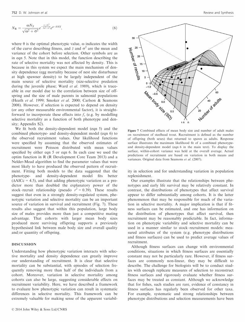
combined phenotype- and density-dependent model (eqn 6) tothe observed recruitment values. Our likelihood functionswere specified by assuming that the observed estimates ofrecruitment were Poisson distributed with mean valuesspecified by either eqn 5 or eqn 6. In each case we used theoptim function in R (R Development Core Team 2013) and aNelder-Mead algorithm to find the parameter values that weremost likely to have produced the observed pattern of recruit-ment. Fitting both models to the data suggested that thephenotype- and density-dependent model fits better(ΔAICc = 4.5), and that adding phenotypic variation as a pre-dictor more than doubled the explanatory power of thestock–recruit relationship (pseudo r2 = 0.39). These resultssuggest that even in a strongly density-regulated system, phe-notypic variation and selective mortality can be an importantsource of variation in survival and recruitment (Fig. 7). Theseresults also suggest that within this population, large bodysize of males provides more than just a competitive matingadvantage. That cohorts with larger mean body sizesproduced more surviving offspring supports a previouslyhypothesised link between male body size and overall qualityand/or quantity of offspring.

DISCUSSION

Understanding how phenotypic variation interacts with selec-tive mortality and density dependence can greatly improveour understanding of recruitment. It is clear that selectivemortality can be substantial, with episodes of selection fre-quently removing more than half of the individuals from acohort. Moreover, variation in selective mortality amongcohorts can also be large, suggesting considerable effects onrecruitment variability. Here, we have described a frameworkto evaluate how phenotypic variation can result in systematicdifferences in selective mortality. This framework can beextremely valuable for making sense of the apparent variabil-

ity in selection and for understanding variation in populationreplenishment.Our examples illustrate that the relationships between phe-

notypes and early life survival may be relatively constant. Incontrast, the distributions of phenotypes that affect survivalappear to differ substantially among cohorts. It is the latterphenomenon that may be responsible for much of the varia-tion in selective mortality. A major implication is that if fit-ness surfaces can be estimated, and one has information onthe distribution of phenotypes that affect survival, thenrecruitment may be reasonably predictable. In fact, informa-tion on phenotypic variability and selective mortality can beused in a manner similar to stock–recruitment models: mea-sured attributes of the system (e.g. phenotype distributionsand fitness surfaces) can be used to predict average values ofrecruitment.Although fitness surfaces can change with environmental

conditions, situations in which fitness surfaces are essentiallyconstant may not be particularly rare. However, if fitness sur-faces are commonly non-linear, they may be difficult todescribe. The challenge for biologists will be to conduct stud-ies with enough replicate measures of selection to reconstructfitness surfaces and rigorously evaluate whether fitness sur-faces may be treated as constant. Although we acknowledgethat for fishes, such studies are rare, evidence of constancy infitness surfaces has regularly been observed for other taxa.For example, systematic and strong relationships betweenphenotype distributions and selection measurements have been

Figure 7 Combined effects of mean body size and number of adult males

on recruitment of steelhead trout. Recruitment is defined as the number

of offspring (both sexes) that returned to spawn as adults. Response

surface illustrates the maximum likelihood fit of a combined phenotype-

and density-dependent model (eqn 6 in the main text). To display the

surface, within-cohort variance was held at the overall average. Actual

predictions of recruitment are based on variation in both means and

variances. Original data from Seamons et al. (2007).



observed in well-replicated studies of selection in populationsof insects (e.g. Weis et al. 1992), birds (e.g. Reed et al. 2006;Brommer & Rattiste 2008; Charmantier et al. 2008), andmammals (e.g. Wilson et al. 2006). These observations suggestthat the general methods described in this study may bewidely applicable, even if constant fitness surfaces are not thenorm. Moreover, when it is clear that fitness surfaces do varywith other features of the local environment (e.g. density orany other measurable characteristic), such effects may beincorporated into the function describing the rate of selectivemortality (e.g. fz can become fz,N in the case of density-depen-dent selection; Appendix S2).When mortality is density dependent, information on phe-

notype distributions and selective mortality can add anotherdimension to traditional stock–recruitment models. Simple,density-dependent models usually do a reasonable job ofdescribing non-linear relationships between density andrecruitment. However, such models typically do a poor job ofexplaining variability in real data (Iles 1994; Myers 2001). Inother words, density-dependent models capture the centraltendency of recruitment, but they cannot explain why certaincohorts deviate from this central tendency. Several studieshave implied that accounting for some forms of phenotypicvariation (particularly changes in the age/size composition ofthe spawning population) in stock–recruitment models canimprove their performance (Marteinsdottir & Thorarinsson1998; Scott et al. 1999; Lucero 2009; Brunel 2010). However,both density dependence and the relationship between pheno-type(s) and survival are often strongly non-linear. Because ofthis, simple approaches to analysing the effects of phenotypeand density on recruitment (e.g. multiple regression) are unli-kely to be adequate. For example, on curvilinear fitness sur-faces, differences in the variances of cohorts can lead to largedifferences in recruitment (eqn 6). For fishes, within-cohortvariance is highly variable among cohorts (from our review,median CV = 23%, range = 2.6–64%), and likely to be a per-sistent source of recruitment variation. By starting with indi-vidual survival probabilities, and accounting for thedistributions of individuals within cohorts, we can generatemodels of density-dependent recruitment that properlyaccount for the non-linear effects of phenotype on survival.

CONCLUSIONS

Our review and synthesis of selection measurements suggeststhat for recruiting cohorts of fishes, most mortality is selectivemortality. The amount of selective mortality is also highlyvariable among cohorts, suggesting that if we have a betterunderstanding of why selective mortality varies, then we canimprove our understanding of recruitment. Through severalempirical examples where selection has been well studied, ouranalyses show that fitness surfaces may be relatively constant,but strongly non-linear. These results suggest that much ofthe variation in mortality during the recruitment process maybe predictable and a direct consequence of variation in thedistribution of phenotypes that are important for survival.The true utility of a framework that describes the combined

effects of phenotypic variation, selective mortality and densitydependence (where applicable) on recruitment is that it will

allow one to evaluate both the short- and long-term conse-quences of variation in phenotypes. For fishes, among-cohortvariation in the distribution of early life traits can be influ-enced by several factors including temperature (Macpherson& Raventos 2005; Sponaugle et al. 2006), parental effects(Heath et al. 1999; McCormick 2006; Johnson et al. 2011),location of larval development (Hamilton et al. 2008; Shima& Swearer 2009) and/or source population (e.g. Post & Prank-evicius 1987). In the short term, knowing the shape of the fit-ness surface will yield insight into how variation in theseenvironmental factors ultimately translates into variation inrecruitment. In the long term, an accurate description of thefitness surface will be useful in that it will allow investigatorsto predict the effects of long-term changes in characteristics oflarvae and juveniles. For example, it is expected that early lifetraits will change in response to factors such as fishery selec-tion (Munch et al. 2005; Walsh et al. 2006; Johnson et al.2011) and climate change (e.g. Munday et al. 2009; Franke &Clemmesen 2011; Baumann et al. 2012). By understandinghow such changes in phenotypes will ultimately affect recruit-ment, we will be able to anticipate how changes in the abioticand biotic environment will affect both the quality of individ-uals in the population, and the population’s capacity for resis-tance and/or resilience to environmental change.

ACKNOWLEDGEMENTS

We thank Robert Warner, Todd Seamons, Liz P�asztor and twoanonymous referees for their helpful comments on an earlierdraft of the manuscript. This work was conducted while D.W.J.was supported by a postdoctoral fellowship from Scripps Insti-tution of Oceanography. During the preparation of this manu-script, both S.S. and B.X.S. were supported in part by grantsfrom the National Oceanic and Atmospheric Administration(NA11NOS4780045 to S.S., NA10OAR4320156 to B.X.S.).

AUTHORSHIP

D.J., K.G.C., S.S. and B.X.S. conceived the study. D.J. wrotethe first draft of the manuscript, and all authors contributedsubstantially to the revisions.

REFERENCES

Anderson, J.T. (1988). A review of size dependent survival during pre-

recruit stages of fishes in relation to recruitment. J. Northwest Atl. Fish.

Sci., 8, 55–66.Bailey, K.M. & Houde, E.D. (1989). Predation on eggs and larvae of marine

fishes and the recruitment problem. In Advances in Marine Biology. (eds

Blaxter, J.H.S., Southward, A.J.). Academic, Press, pp. 1–83.Baumann, H., Talmage, S.C. & Gobler, C.J. (2012). Reduced early life

growth and survival in a fish in direct response to increased carbon

dioxide. Nature Clim. Change, 2, 38–41.Benton, T.G., Plaistow, S.J. & Coulson, T.N. (2006). Complex population

dynamics and complex causation: devils, details and demography. Proc.

R. Soc. B, 273, 1173–1181.Beverton, R.J.H. & Holt, S.J. (1957). On the dynamics of exploited fish

populations. In: Fishery Investigations Series 2: Sea Fisheries, 19,

533pp.

Bjørnstad, O.N. & Hansen, T.F. (1994). Individual variation and

population dynamics. Oikos, 69, 167–171.



Brommer, J.E. & Rattiste, K. (2008). ‘Hidden’ reproductive conflict

between mates in a wild bird population. Evolution, 62, 2326–2333.Brunel, T. (2010). Age-structure-dependent recruitment: a meta-analysis

applied to Northeast Atlantic fish stocks. ICES J. Mar. Sci., 67, 1921–1930.

Cappuccino, N. & Price, P.W. (1995). Population Dynamics: New

Approaches and Synthesis. Academic Press, San Diego, CA, USA.

Carlson, S.M. & Seamons, T.R. (2008). A review of quantitative genetic

components of fitness in salmonids: implications for adaptation to

future change. Evol. Appl., 1, 222–238.Charmantier, A., McCleery, R.H., Cole, L.R., Perrins, C., Kruuk, L.E.B.

& Sheldon, B.C. (2008). Adaptive phenotypic plasticity in response to

climate change in a wild bird population. Science, 320, 800–803.Einum, S. & Fleming, I.A. (2000). Highly fecund mothers sacrifice

offspring survival to maximize fitness. Nature, 405, 565–567.Einum, S., Robertsen, G. & Fleming, I.A. (2008). Adaptive landscapes

and density-dependent selection in declining salmonid populations:

going beyond numerical responses to human disturbance. Evol. Appl.,

1, 239–251.Ellner, S.P., Geber, M.A. & Hairston, N.G. (2011). Does rapid evolution

matter? Measuring the rate of contemporary evolution and its impacts

on ecological dynamics. Ecol. Lett., 14, 603–614.Endler, J.A. (1980). Natural selection on color patterns in Poecilia

reticulata. Evolution, 34, 76–91.Endler, J.A. (1986). Natural Selection in the Wild. Princeton University

Press, Princeton, NJ, USA.

Ezard, T.H.G., Cot�e, S.D. & Pelletier, F. (2009). Eco-evolutionary

dynamics: disentangling phenotypic, environmental and population

fluctuations. Phil. Trans. R. Soc. B, 364, 1491–1498.Falconer, D.S. & Mackay, T.F.C. (1996). Introduction to Quantitative

Genetics. Longman, England.

Franke, A. & Clemmesen, C. (2011). Effect of ocean acidification on early

life stages of Atlantic herring (Clupea harengus L.). Biogeosciences

Discussions, 8, 7097–7126.Fukushima, M., Quinn, T.J. & Smoker, W.W. (1998). Estimation of eggs

lost from superimposed pink salmon (Oncorhynchus gorbuscha) redds.

Can. J. Fish. Aquat. Sci., 55, 618–625.Gaillard, J.-M., Festa-Bianchet, M., Yoccoz, N.G., Loison, A. & Toigo,

C. (2000). Temporal variation in fitness components and population

dynamics of large herbivores. Annu. Rev. Ecol. Syst., 31, 367–393.Good, S.P., Dodson, J.J., Meekan, M.G. & Ryan, D.A. (2001). Annual

variation in size-selective mortality of Atlantic salmon (Salmo salar)

fry. Can. J. Fish. Aquat. Sci., 58, 1187–1195.Grorud-Colvert, K. & Sponaugle, S. (2011). Variability in water

temperature affects trait-mediated survival of a newly settled coral reef

fish. Oecologia, 165, 675–686.Hairston, N.G., Ellner, S.P., Geber, M.A., Yoshida, T. & Fox, J.A.

(2005). Rapid evolution and the convergence of ecological and

evolutionary time. Ecol. Lett., 8, 1114–1127.Hamilton, S.L. (2008). Larval history influences post-metamorphic

condition in a coral-reef fish. Oecologia, 158, 449–461.Hamilton, S.L., Regetz, J. & Warner, R.R. (2008). Postsettlement survival

linked to larval life in a marine fish. Proc. Natl Acad. Sci., 105, 1561–1566.

Heath, D.D., Fox, C.W. & Heath, J.W. (1999). Maternal effects on

offspring size: variation through early development of chinook salmon.

Evolution, 53, 1605–1611.Hixon, M.A. & Jones, G.P. (2005). Competition, predation, and density-

dependent mortality in demersal marine fishes. Ecology, 86, 2847–2859.Hixon, M.A. & Webster, M.S. (2002). Density dependence in reef fish

populations. In: Coral Reef Fishes: Dynamics and Diversity in a

Complex Ecosystem (ed Sale, P.F.). Academic Press, San Diego, CA,

USA, pp. 303–325.Houde, E. (1987). Fish early life dynamics and recruitment variability.

Am. Fish. Soc. Symp., 2, 17–29.Houde, E.D. (2008). Emerging from Hjort’s Shadow. Journal of

Northwest Atlantic Fishery Science, 41, 53–70.

Iles, T.C. (1994). A review of stock-recruitment relationships with

reference to flatfish populations. Neth. J. Sea Res., 32, 399–420.Janzen, F.J. & Stern, H.S. (1998). Logistic regression for empirical studies

of multivariate selection. Evolution, 52, 1564–1571.Johnson, D.W. (2008). Combined effects of condition and density on

post-settlement survival and growth of a marine fish. Oecologia, 155,

43–52.Johnson, D.W., Christie, M.R. & Moye, J. (2010). Quantifying

evolutionary potential of marine fish larvae: heritability, selection, and

evolutionary constraints. Evolution, 64, 2614–2628.Johnson, D.W., Christie, M.R., Moye, J. & Hixon, M.A. (2011). Genetic

correlations between adults and larvae in a marine fish: potential effects

of fishery selection on population replenishment. Evol. Appl., 4, 621–633.

Johnson, D.W., GrorudColvert, K., Rankin, T.L. & Sponaugle, S. (2012).

Measuring selective mortality from otoliths and similar structures: a

practical guide for describing multivariate selection from cross-sectional

data. Mar. Ecol. Prog. Ser., 471, 151–163.Kokko, H. & L�opez-Sepulcre, A. (2007). The ecogenetic link between

demography and evolution: can we bridge the gap between theory and

data? Ecol. Lett., 10, 773–782.Lande, R. (1976). Natural selection and random genetic drift in

phenotypic evolution. Evolution, 30, 314–334.Lande, R. (1981). Models of speciation by sexual selection on polygenic

traits. PNAS, 78, 3721–3725.Lande, R. & Arnold, S.J. (1983). The measurement of selection on

correlated characters. Evolution, 37, 1210–1226.Lucero, Y. (2009). A multivariate stock–recruitment function for cohorts

with sympatric subclasses: application to maternal effects in rockfish

(genus Sebastes). Can. J. Fish. Aquat. Sci., 66, 557–564.Macpherson, E. & Raventos, N. (2005). Settlement patterns and post-

settlement survival in two Mediterranean littoral fishes: influences of

early-life traits and environmental variables. Mar. Biol., 148, 167–177.Marchinko, K.B. (2009). Predation’s role in repeated phenotypic and

genetic divergence of armor in threespine stickleback. Evolution, 63,

127–138.Marteinsdottir, G. & Thorarinsson, K. (1998). Improving the stock-

recruitment relationship in Icelandic cod (Gadus morhua) by including

age diversity of spawners. Can. J. Fish. Aquat. Sci., 55, 1372–1377.McCormick, M.I. (2006). Mothers matter: crowding leads to stressed

mothers and smaller offspring in marine fish. Ecology, 87, 1104–1109.McNeil, W.J. (1964). Redd superimposition and egg capacity of pink

salmon spawning beds. Journal of the Fisheries Board of Canada, 21,

1385–1396.Meekan, M. & Fortier, L. (1996). Selection for fast growth during the

larval life of Atlantic cod Gadus morhua on the Scotian Shelf. Mar.

Ecol. Prog. Ser., 137, 25–37.Metcalf, C.J.E. & Pavard, S. (2007). Why evolutionary biologists should

be demographers. Trends Ecol. Evol., 22, 205–212.Miller, T.J., Crowder, L.B., Rice, J.A. & Marschall, E.A. (1998). Larval

size and recruitment mechanisms in fishes: Toward a conceptual

framework. Canadian Journal of Fisheries and Aquatic Sciences, 45,

1657–1670.Mitchell-Olds, T. & Shaw, R.G. (1987). Regression analysis of natural

selection: statistical inference and biological interpretation. Evolution,

41, 1149–1161.Morrissey, M.B. & Hadfield, J.D. (2012). Directional selection in

temporally replicated studies is remarkably consistent. Evolution, 66,

435–442.Munch, S.B., Walsh, M.R. & Conover, D.O. (2005). Harvest selection,

genetic correlations, and evolutionary changes in recruitment: one less

thing to worry about? Can. J. Fish. Aquat. Sci., 62, 802–810.Munday, P.L., Donelson, J.M., Dixson, D.L. & Endo, G.G.K. (2009).

Effects of ocean acidification on the early life history of a tropical

marine fish. Proc. R. Soc. B, 276, 3275–3283.Murdoch, W.W. (1994). Population regulation in theory and practice.

Ecology, 75, 271–287.



Myers, R.A. (2001). Stock and recruitment: generalizations about

maximum reproductive rate, density dependence, and variability using

meta-analytic approaches. ICES J. Mar. Sci., 58, 937–951.Myers, R.A. & Cadigan, N.G. (1993). Density-dependent juvenile

mortality in marine demersal fish. Can. J. Fish. Aquat. Sci., 50, 1576–1590.

Osenberg, C.W., St. Mary, C.M., Schmitt, R.J., Holbrook, S.J., Chesson,

P. & Byrne, B.. (2002). Rethinking ecological inference: density

dependence in reef fishes. Ecol. Lett., 5, 715–721.Pelletier, F., Garant, D. & Hendry, A.P. (2009). Eco-evolutionary

dynamics. Phil. Trans. R. Soc. B, 364, 1483–1489.Perez, K.O. & Munch, S.B. (2010). Extreme selection on size in the early

lives of fish. Evolution, 64, 2450–2457.Phillips, P.C. & Arnold, S.J. (1989). Visualizing multivariate selection.

Evolution, 43, 1209–1222.Post, J.R. & Prankevicius, A.B. (1987). Size-selective mortality in young-

of-the-year yellow perch (Perca flavescens): evidence from otolith

microstructure. Can. J. Fish. Aquat. Sci., 44, 1840–1847.Press, S.J. (2012). Applied Multivariate Analysis: Using Bayesian and

Frequentist Methods of Inference, 2nd edn. Courier Dover Publications,

Mineola, NY, USA.

R Development Core Team. (2013). R: A language and environment for

statistical computing. R Foundation for Statistical Computing, Vienna,

Austria.

Rankin, T.L. & Sponaugle, S. (2011). Temperature influences selective

mortality during the early life stages of a coral reef fish. PLoS ONE, 6,

e16814.

Reed, T.E., Wanless, S., Harris, M.P., Frederiksen, M., Kruuk, L.E.B. &

Cunningham, E.J.A. (2006). Responding to environmental change:

plastic responses vary little in a synchronous breeder. Proc. R. Soc. B,

273, 2713–2719.Reznick, D.N. & Bryga, H. (1987). Life-history evolution in guppies

(Poecilia reticulata): 1. phenotypic and genetic changes in an

introduction experiment. Evolution, 41, 1370–1385.Ricker, W. (1954). Stock and recruitment. J. Fish. Res. Board Can., 11,

559–609.Rose, K.A., Cowan, J.H., Winemiller, K.O., Myers, R.A. & Hilborn, R.

(2001). Compensatory density dependence in fish populations:

importance, controversy, understanding and prognosis. Fish Fish., 2,

293–327.Ruel, J.J. & Ayres, M.P. (1999). Jensen’s inequality predicts effects of

environmental variation. Trends Ecol. Evol., 14, 361–366.Saccheri, I. & Hanski, I. (2006). Natural selection and population

dynamics. Trends Ecol. Evol., 21, 341–347.Schoener, T.W. (2011). The newest synthesis: understanding the interplay

of evolutionary and ecological dynamics. Science, 331, 426–429.Scott, B., Marteinsdottir, G. & Wright, P. (1999). Potential effects of

maternal factors on spawning stock–recruitment relationships under

varying fishing pressure. Can. J. Fish. Aquat. Sci., 56, 1882–1890.Seamons, T.R., Bentzen, P. & Quinn, T.P. (2007). DNA parentage

analysis reveals inter-annual variation in selection: results from

19 consecutive brood years in steelhead trout. Evol. Ecol. Res., 9, 409–431.

Shima, J.S. & Swearer, S.E. (2009). Larval quality is shaped by matrix

effects: implications for connectivity in a marine metapopulation.

Ecology, 90, 1255–1267.Shima, J.S., Osenberg, C.W., St Mary, C.M. & Rogers, L. (2006).

Implication of changing coral communities: do larval traits or habitat

features drive variation in density-dependent mortality and recruitment

of juvenile reef fish. Proceedings of the 10th International Coral Reef

Symposium, Okinawa, Japan, pp. 226–231.

Siepielski, A.M., DiBattista, J.D. & Carlson, S.M. (2009). It’s about time:

the temporal dynamics of phenotypic selection in the wild. Ecol. Lett.,

12, 1261–1276.Smallegange, I.M. & Coulson, T. (2013). Towards a general, population-

level understanding of eco-evolutionary change. Trends Ecol. Evol., 28,

143–148.Smith, C.C. & Fretwell, S.D. (1974). The optimal balance between size

and number of offspring. Am. Nat., 108, 499–506.Smoker, W.W., Gharrett, A.J., Stekoll, M.S. & Taylor, S.G. (2000).

Genetic variation of fecundity and egg size in anadromous pink salmon

Oncorhynchus gorbuscha Walbaum. Alaska Fishery Research Bulletin, 7,

44–50.Sogard, S.M. (1997). Size-selective mortality in the juvenile stage of

teleost fishes: a review. Bull. Mar. Sci., 60, 1129–1157.Sponaugle, S. (2010). Otolith microstructure reveals ecological and

oceanographic processes important to ecosystem-based management.

Environ. Biol. Fishes, 89, 221–238.Sponaugle, S., Grorud-Colvert, K. & Pinkard, D. (2006). Temperature-

mediated variation in early life history traits and recruitment success of

the coral reef fish Thalassoma bifasciatum in the Florida Keys. Mar.

Ecol. Prog. Ser., 308, 1–15.Steele, D.B., Siepielski, A.M. & McPeek, M.A. (2011). Sexual selection

and temporal phenotypic variation in a damselfly population. J. Evol.

Biol., 24, 1517–1532.Thompson, J.N. (1998). Rapid evolution as an ecological process. Trends

Ecol. Evol., 13, 329–332.Van Tienderen, P.H. (2000). Elasticities and the link between

demographic and evolutionary dynamics. Ecology, 81, 666–679.Van Valen, L. (1965). Selection in natural populations. iii. measurement

and estimation. Evolution, 19, 514–528.Vance, R.R. (1973). On reproductive strategies in marine benthic

invertebrates. Am. Nat., 107, 339–352.Walsh, M.R., Munch, S.B., Chiba, S. & Conover, D.O. (2006).

Maladaptive changes in multiple traits caused by fishing: impediments

to population recovery. Ecol. Lett., 9, 142–148.Ward, D.L., Slaney, P.A., Facchin, A.R. & Land, R.W. (1989). Size-

biased survival in steelhead trout (Oncorhynchus mykiss): Back-

calculated lengths from adults’ scales compared to migrating smolts at

the Keogh River, British Columbia. Canadian Journal of Fisheries and

Aquatic Sciences, 46, 1853–1858.Weis, A.E., Abrahamson, W.G. & Andersen, M.C. (1992). Variable

selection on Eurosta’s gall size, i: the extent and nature of variation in

phenotypic selection. Evolution, 46, 1674–1697.Wilson, A.J., Pemberton, J.M., Pilkington, J.G., Coltman, D.W., Mifsud,

D.V., Clutton-Brock, T.H. et al. (2006). Environmental coupling of

selection and heritability limits evolution. PLoS Biol., 4, e216.

SUPPORTING INFORMATION

Additional Supporting Information may be downloaded viathe online version of this article at Wiley Online Library(www.ecologyletters.com).

Editor, Mikko HeinoManuscript received 26 December 2013First decision made 31 January 2014Second decision made 18 February 2014Manuscript accepted 24 February 2014



johnson et al 2014 plasticidad fenotipica mortandad selectiva peces variacion

Documents