jobs for justice(s): corruption in the supreme court of … · corruption in the supreme court of...

Jobs for Justice(s):Corruption in the Supreme Court of India

Madhav S. Aney1, Shubhankar Dam2, and Giovanni Ko∗31School of Economics, Singapore Management University

2Columbia Law School and School of Law, University of Portsmouth3School of Social Sciences, Nanyang Technological University Singapore

June 13, 2018

Abstract

We investigate whether judges respond to pandering incentives by ruling in favour of thegovernment in the hope of receiving jobs after retiring from the Court. We construct a datasetof all reported Supreme Court of India cases involving the government from 1999 till 2014,with an indicator for whether the decision was in its favour or not. We find that pander-ing incentives have a causal effect on judicial decision-making, where we define panderingincentives as being jointly determined by 1) the salience of the case (exogenously determinedby a system of random allocation of cases) and 2) whether the judge retires with enoughtime left in a government’s term to be rewarded with a prestigious job (since the date ofretirement is exogenously determined by law to be their 65th birthday). We also find thatauthoring judgements in favour of the government is positively associated with the likelihoodof being appointed to a prestigious post-Supreme Court job. These findings suggest the pres-ence of corruption in the form of government influence over judicial decisions that seriouslyundermines judicial independence. 1

Keywords: judicial decision-making, corruption, separation of powers, career concerns,public sector incentives

JEL codes: D73, H11, K40

∗Corresponding author. [email protected]. +65 6790 6736. 14 Nanyang Drive, Singapore 637332.1We thank Konrad Burchardi, Parkash Chander, Davin Chor, Dhammika Dharmapala, Steven Durlauf, Alexan-

der Christoph Fischer, Tom Ginsburg, William H.J. Hubbard, Brian P. Kennedy, Nuarpear Lekfuangfu, Lin Feng,Vikramaditya Khanna, Lawrence Lessig, Anirban Mitra, Omer Moav, Abhiroop Mukhopadhyay, Mark Ramseyer,Yona Rubinstein, Tom Sargent, Shekhar Shah, Prakarsh Singh, Sujata Visaria, Yasutora Watanabe and seminarparticipants at Singapore Management University, City University of Hong Kong, Hong Kong University of Scienceand Technology, London School of Economics, National University of Singapore, IDC Herzliya, Bar-Ilan University,National Council of Applied Economic Research, Delhi School of Economics, Australasian Public Choice Confer-ence, ISI Annual Conference on Growth and Development, Colloquium on the Supreme Court of India organised byJindal Global Law School, ISI Delhi, American Law and Economics Association Conference, Empirical Enquiriesinto the Indian Judicial System at the University of Chicago Center in Delhi, SMU ECON204 students from 2017and 2018 cohorts, and one anonymous referee for valuable comments and suggestions. We also thank our projectmanager Dominic Liew and research assistants Alwyn Loy, Chong Shou Yu, Charlene Chow, Glenda Lim, KartikSingh, Nicole Chan, Nicole Ann Lim, Persis Hoo, Shirlene Leong and Teo Ting Wei. The views expressed here aresolely those of the authors.

1

1 Introduction

The fact that many public servants have careers after their tenure in public service has long

been thought to create conflicts of interest.2 In response to this concern, many countries

constrain former public servants by requiring a cooling-off period after retirement before

they seek fresh employment. However, such constraints rarely apply to retired judges.3 In

countries with term limits for judges, it is common for retired judges to go on to have careers

in the public and private sectors. This practice raises the possibility that the prospect of post-

retirement appointments influences judicial decision making. If true, this compromises the

idea of a fair and independent judiciary,4 a critical feature of a well-functioning representative

democracy. In this paper, we investigate the practice of awarding government jobs to retired

judges, and show that the concerns surrounding it are in fact valid.

We examine this practice in the context of India. Over the last two decades, it has

become common for retiring Supreme Court Justices in India to be appointed to prestigious

government positions. This has been criticised as leading to a bias in favour of the government

when judges decide cases with high stakes that are important to the government.5 In this

context, critics allege that corruption takes the form of the following quid-pro-quo: judges

pander to the government by ruling in its favour and in exchange, the government rewards

judges who have done so with jobs. This raises a natural question that we confront in

this paper: do judges actually respond to pandering incentives by ruling in favour of the

government to secure post-retirement jobs? In this paper, we answer this question in the

affirmative.

To do so, we constructed a novel dataset of cases decided by the Supreme Court of India

between 1999 and 2014 involving the government. We analysed the full text of the judgements

and coded whether the government won or lost the case.

The key identification challenge is that a correlation between favourable judicial decisions

and government appointments after retirement may be driven simply by characteristics of

judges such as, for example, their suitability for particular appointments or their ideology,

rather than by manipulation of judicial decisions to secure such appointments. As such,

judicial decision-making may be invariant to incentives and may merely reveal a judge’s

“type” rather than indicate the presence of corruption. To address this concern we focus on

2There is an emerging empirical literature that suggests that individuals with government experience derivesubstantial value as lobbyists from their connections to serving politicians. See for example Bertrand, Bombardini,and Trebbi (2014) and Vidal, Draca, and Fons-Rosen (2012). It is therefore plausible that the prospect of suchlobbying roles affects their behaviour when they serve in government. See Dal Bo (2006) for a review of the literatureon revolving doors and regulatory capture.

3See chapter 3 of Garupa and Ginsburg (2015) for an extensive discussion of the practice of awarding jobs tojudges across different countries.

4Judicial independence is typically defined as independence from the parties to the dispute, that is, the judgedoes not expect his welfare to be affected by whether he decides in favour of one party or the other. More specificallyit is also seen as independence from government influence when it comes to judicial decision making. See Ramseyer(1998) for a discussion of the idea of judicial independence and a survey of the literature.

5We present some of the public discourse surrounding this issue in section 7.

2

judicial behaviour and attempt to isolate the causal effect of pandering incentives on judicial

decision making.

In our framework, the exposure of a judge to pandering incentives in a case is jointly

determined by 1) whether the case is salient and 2) whether the judge retires with enough

time (at least 16 months) left in a government’s term to be rewarded with a prestigious job.

The institutional architecture of the Supreme Court of India has two unique features that

ensure that these pandering incentives are plausibly exogenous. First, salience, i.e., whether

the case is of special importance to the government, is plausibly exogenous because cases are

randomly assigned to judges. Second, the time between the retirement of a judge and the

date of the next election is exogenous in our sample for two reasons: judges must retire on

their 65th birthday; all governments served their full terms and elections were regularly held

at 5-year intervals.

We therefore use a difference-in-differences approach where the two dimensions of variation

are the salience of a case and the time between a judge’s retirement and the next election. We

can think of benches with judges retiring long before an election as “treatment” benches and

those with judges retiring shortly before an election as “control” benches. Our identification

strategy relies on the assumption that, although there could be differences between salient

and non-salient cases due to factors other than pandering incentives, these differences do not

vary between treatment and control benches.

Using this methodology, we find that judges who have pandering incentives are more likely

to rule in favour of the government. We interpret this result as the causal effect of pandering

incentives on judicial behaviour.

Furthermore, we attempt to characterise the channel through which pandering incentives

work and find that the mechanism consists of actually being the author of judgements rather

than simply being on a bench that decides the case in favour of the government. On the

“rewards” side, we show that authoring decisions in salient cases in favour of the government

is positively correlated with whether or not the judge is appointed to prestigious post-Supreme

Court jobs. This correlation remains robust to instrumenting favourable decisions authored

in salient cases with the number of salient cases decided by the judge. Similar to the results

on the nexus between bureaucrats and politicians in India presented in Iyer and Mani (2012),

these results suggest that pandering to the government may be a path to a post-retirement

appointment.

A large literature analyses the question of judicial independence. In the context of the

US, Ashenfelter, Eisenberg, and Schwab (1995) find that there is no effect of the ideology

of the president who appoints a judge on judicial decisions in federal trial courts. Ramseyer

and Rasmusen (1997) present evidence suggesting that in Japan, where judges are appointed

to the national judiciary and not to specific courts, deciding against the ruling party leads

to worse assignments when judges are transferred. In Argentina, Iaryczower, Spiller, and

Tommasi (2002) find that judges do decide against the government, and the likelihood of

doing so is higher when the government is unlikely to survive. Helmke (2002) also finds

3

similar results that suggest there is a strategic dimension to judicial decision making. Black

and Owens (2016) show that US circuit judges, who have a good chance of being appointed

to the US Supreme Court, are more likely to decide in line with the president’s ideology

when a vacancy arises on the Supreme Court. Similar results are documented in Epstein,

Landes, and Posner (2013). On the other hand Salzberger and Fenn (1999) find that in the

UK, reversing favourable lower court decisions does not harm the chances of promotion to

the House of Lords from the Court of Appeal. Our paper adds to this literature by using the

combination of random allocation of cases and fixed retirement dates to rule out ideology-

based explanations of judicial behaviour and isolate the causal effect of incentives on judicial

decisions.

Our paper also contributes to the growing empirical literature on legal realism that exam-

ines how judicial decisions are affected by factors unrelated to legal reasoning. Lim, Snyder,

and Stromberg (2015) show that sentence lengths are increased significantly by newspaper

coverage of the case. Chen, Moskowitz, and Shue (2016) document a negative autocorrela-

tion in refugee asylum court cases unrelated to their merits, suggesting that the gambler’s

fallacy is at work – judges underestimate the likelihood of sequential streaks occurring by

chance. Boyd, Epstein, and Martin (2010) document the existence of systematic differences

in decisions of male and female judges. Our paper adds economic incentives in the form of

career concerns to the list of the factors that may affect judicial decisions. In attempting to

understand of how career concerns affect outcomes in the public sector, our paper comple-

ments the empirical literature on career concerns which focuses mostly on incentives within

the firm, such as executive compensation.6

Finally, our paper is related to the empirical literature on identifying and measuring

corruption at an aggregate institutional level.7 More specifically, our paper is related to the

literature on corruption that seeks to understand the determinants of corruption and what

can be done about it. Bobonis, Fuertes, and Schwabe (2016) document how variation in

the time at which a municipal government in Puerto Rico is audited, relative to the date of

election, enables voters to identify corruption and select responsive politicians. Similar results

are seen in Ferraz and Finan (2008).8 As highlighted in a survey by Olken and Pande (2012),

6Notable exceptions are Schneider (2005) and Li and Zhou (2005). For an insightful discussion of incentivereforms in the public sector, see Mookherjee (1997). For theoretical work on the effect of career concerns of judgesand lawyers on litigation see Levy (2005) and Ferrer (2015).

7Surveys include Banerjee, Hanna, and Mullainathan (2012), Pande (2007), and Sukhtankar and Vaishnav (2015).See Lessig (2013a) and Lessig (2013b) for a discussion of the idea of institutional corruption in law. The notionof institutional corruption was originally developed by Thompson (1995) to explain the US Congress’ deviationfrom its proper purpose because of the influence of several systemic features of the legislative process. Applicationsinclude Williams (2013) in the context of dissemination of research for the benefit of funders; Youngdahl (2013)and Fox (2013) in the context of misalignment of incentives in the design and sale of financial products; Rodwin(2013) in the context of the interaction between pharmaceutical firms and prescribing physicians; Mendonca (2013)and Laver (2014) in the context of judicial independence in Latin America.

8See Callen and Long (2015), Ferraz and Finan (2011), and Niehaus and Sukhtankar (2013) for more examplesof settings where corruption is identified as arising from specific incentives. See Fisman and Miguel (2007) for anexample of how both social norms and incentives in the form of legal enforcement may shape corruption, and Olken(2007) for the effectiveness of government audits and grassroots participation on corruption in road projects in

4

this literature reinforces the centrality of incentives in shaping corruption. Since corruption

in these settings arises from poorly designed incentives, a strength of this literature is the

existence of clear policy implications.

In line with the empirical literature on corruption, we present statistical evidence of cor-

ruption, that is, we find that the existence of corruption is the most parsimonious and com-

pelling explanation that fits the data at an aggregate level. Given the statistical nature of

our study we are unable to identify the presence of corruption in a particular case or by

a particular judge. Therefore, our use of the term corruption should not be understood to

refer an individual instance of corruption by a particular judge. It is also important to note

that the incentives that shape judicial behaviour in our setting are not necessarily finan-

cial in nature: the attraction of these jobs may be largely due to the influence the holders

continue to wield on policy matters, rather than just the salary and perks associated with

these jobs.9 This is different from the type of corruption that arises from bribes from the

private sector, documented for example in Fisman, Schulz, and Vig (2014) who show that

political candidates that win elections in India show an increase in asset growth relative to

the runners-up. Instead, in our context, corruption arises from the government itself trying

to influence judicial decision-making.

Our paper is of interest for three reasons. First, our paper identifies the causal effect

of career-concern incentives on judicial decision making. Second, we identify corruption in

a very high-profile institution subject to intense public scrutiny, where one would expect

it to be subtle and hard to detect. Finally, the kind of corruption we uncover is systemic

in nature and shaped by incentives, rather than being a “type”-based phenomenon that is

created by bad behaviour of some “rotten apples”. Hence, our findings suggest a clear role

for institutional reform in addressing the problem.

The rest of the paper is organised as follows. We describe the institutional background of

the Supreme Court of India in section 2, the data in section 3 and the empirical strategy in

section 4. In section 5, we present our main results about the presence of pandering, together

with robustness checks. In section 6, we explore the channels through which pandering occurs.

In section 7, we present evidence that the government rewards pandering with post-Supreme

Court jobs. We provide concluding remarks in section 8.

2 Institutional background

The Supreme Court of India is the apex court for the largest common law judicial system

in the world (Chandra, Hubbard, and Kalantry 2017). It decides both appeals from lower

Indonesia.9We follow the Bardhan (1997) definition of corruption as the use of public office for private gain rather than the

narrower definition in Shleifer and Vishny (1993) of corruption as the sale of government property for personal gain.Moreover, the term corruption used in this article should not be read as meeting the legal standards prescribed inthe Prevention of Corruption Act, 1988, India. Instead, it is intended to be understood in the way it is ordinarilyused in the English language.

5

courts and fresh petitions. Compared to supreme courts in other countries, it has a very high

case load. This makes the Supreme Court of India an outlier when compared to Supreme

Courts of other countries, when it comes to access and the number of decisions (Green and

Yoon 2016).

In response to perceived inaction by the executive and the legislature, the Supreme Court

has expanded its remit to matters traditionally within the purview of those branches of gov-

ernment. It routinely strikes down actions by government agencies at all levels and issues

orders on policy matters as diverse as pollution, sexual harassment, etc. As noted by Robin-

son (2013), “despite the range of matters, or perhaps partly because of this diverse and

heavy workload, the Indian Supreme Court has become well known for both its intervention-

ism and creativity.” Unlike the US Supreme Court, which is chiefly concerned with norm

elaboration, Chandra, Hubbard, and Kalantry (2017) show that the Indian Supreme Court

also emphasises the goal of correcting errors case-by-case and thus regularly overturns lower

court decisions. As such, the court is relatively unconstrained in how it decides cases. This

discretion potentially creates an opening for other factors, such as pandering incentives, to

play a role in decision making.

Since 2008, the Constitution of India provides for up to 31 Supreme Court Justices.10

Between 1986 and 2008, the number was limited to 26. However, the actual number of judges

has always been less than 31, with the number in January 2017 being 23. The Chief Justice

of India (henceforth CJI) is the most senior Justice of the Court with additional powers in

the appointment of Justices and the allocation of exceptional cases, as discussed below.

2.1 Allocation of cases

In the Supreme Court of India, a bench is a group of judges who jointly hear and decide a

case. Benches are always composed of at least two judges. Ordinarily, a case is heard by a

two-judge bench, but in the uncommon occasions when the two judges disagree or the case

is of exceptional importance, the CJI constitutes a larger bench of three or more judges to

hear that particular case.

Before 1994, the allocation of cases to benches was at the discretion of the Registry of the

Supreme Court. There was widespread suspicion that this discretion led to “bench-hunting”,

i.e., colllusion between lawyers and the Registry to manipulate the allocation of cases to more

favourable benches. In response to this problem, the Supreme Court switched to a system

of random computerised allocation of cases to benches. In private correspondence with the

authors, a former Registrar General of the Supreme Court who was in service when the new

system was introduced, described the change as follows:

Computerized system of filing and processing with random system of allocation of

petitions to different benches was done with that end that is to save on manual

10See Robinson (2013) and Chandra, Hubbard, and Kalantry (2017) for an insightful exposition of the institutionalbackground of the Supreme Court of India.

6

labour, bring more speed and efficiency. [. . . ] At the same time it also eliminated

the possibility of “forum shopping” or in other words “bench hunting” by lawyers.

The Handbook of the Supreme Court also emphasises that the allocation of cases to benches

by the current system is manipulation-proof, stating that

Since the allocation is made by computer, [. . . ] there is no scope for any Bench-

Hunting. (Section VI.A.i)

Since benches composed of three or more judges are constituted by the Chief Justice to

hear particular cases, the composition of the benches in these cases is endogenous to case

characteristics and we drop such cases from our analysis. Therefore, our sample is composed

solely of cases decided by two-judge benches.11

2.2 Appointment and retirement of judges

Since the mid-1990s, in response to calls for increased judicial independence, the appointment

of judges to the Supreme Court has been the exclusive prerogative of the Supreme Court

itself.12 The CJI, heading a panel composed of other Supreme Court Justices, appoints new

Justices from a pool of (state-level) High Court judges and, in exceptional cases, eminent

Supreme Court lawyers. Therefore, unlike courts such as the US Supreme Court, the executive

and legislative branches of government play no active role in the appointment process. The

appointment of the CJI is mechanical by convention: at any given time, he is the judge with

the longest tenure in the Supreme Court.13

According to Article 124 of the Indian constitution, Supreme Court Justices must retire

from the Court on their 65th birthday. Hence, their retirement date is exogenously determined

by their date of birth.14

After retiring from the Supreme Court, judges are constitutionally barred from practising

law in any Indian court. Many continue to work as arbitrators in private disputes or as mem-

bers of government commissions. The Union government of India (henceforth government) is

the largest employer of ex-Supreme Court judges. Appointments to government positions are

considered prestigious and desirable by judges, as these enable them to continue influencing

11One potential concern is that cases decided during our sample period were actually allocated to benches beforethe randomisation system was introduced in 1996. This is not a concern for our sample since, in every case, at leastone judge was appointed after 1996, so that the bench must have been constituted after the change.

12This change was enacted by the Supreme Court itself in its decision on the Supreme Court Advocates-onRecord Association vs Union of India case of 1993. In 2015 the government amended the Indian Constitutionto wrest some of the power of judicial appointment from the Supreme Court. However, in a case where thisconstitutional amendment was challenged, the Supreme Court struck it down as being unconstitutional. As a resultthe court continues to control the appointment of judges.

13Since the Supreme Court Advocates-on Record Association vs Union of India case of 1993, there has beenno deviation from this convention. Note that although there have been female Supreme Court Justices, we usemasculine pronouns throughout when referring to judges since the court has been overwhelmingly composed ofmen.

14In principle, judges could choose to retire earlier than this, but this only happened for one judge in our sampleperiod. We discuss our treatment of this case in section 3.

7

policy. Due to their prestige, competition for these positions is fierce. These appointments

are made by the executive and are consequently politically driven. This appointment process

is not transparent and is widely believed to be subject to lobbying by judges and internal

machinations within the government.

Hence, although the government has no active role in appointing judges to the Supreme

Court, it wields substantial influence over them by controlling their post-Supreme Court job

prospects, as we demonstrate in later sections. This is in contrast to the US, where the

appointment process to the Supreme Court is heavily politicised but the government wields

little influence over judges once their appointment is finalised. The two systems differ in how

the government tries to influence the Supreme Court: in the US, it does so by manipulating

the type of judges who are appointed to the Court; in India, it does so by incentivising judges

to manipulate their actions through control of post-retirement job prospects.

3 Data

In this section, we describe the sources and features of the data we use in this paper. We

use three kinds of data: information about cases decided by the Supreme Court, information

about judges’ tenures in the Court and information on the jobs they received after retirement

from the Court.

3.1 Case data

The Supreme Court of India has a very high case load. In the 15 years between 1999 and 2014,

the court delivered approximately 22,500 decisions that were reported.15 In this section, we

describe the restrictions we place on reported cases for generating our sample.

Using the SCC Online database, we collected the decisions of the Supreme Court between

1999 and 2014.16 We use this time period since the governments elected between 1999–2014

have served out their full terms and elections have occured every five years in this period,

and this will be a key part of our identification strategy.17

Our sample is composed of all cases that satisfy the following criteria:

• We search for judgements and orders where the “Union of India” or “Ministry” of the

Union of India (equivalent to a department of the US federal government) appear as one

15In our sample period 114,448 cases were admitted for full hearing. See Indian Judiciary Annual Report 2015-16 pp 54-55. The number of reported decisions is lower than this since each decision may resolve multiple casesadmitted for full hearing. This is because cases involving similar facts and legal questions are often clubbed togetherand heard by the same bench, and resolved within one decision. The rest of the paper uses the word “case” tocollectively refer to all cases that are clubbed together in a decision. Additionally, not all decisions are reported bySCC Online, such as those involving short orders or insignificant discussions of the law.

16SCC Online is widely acknowledged to be the most comprehensive database of Supreme Court of India cases,used by lawyers and legal scholars.

17There were 3 elections between 1996 (when the randomisation of case allocation was introduced) and the startof our sample in 1999 with none of the governments serving their full term.

8

of the parties. This leaves us with the full text of 2,605 cases involving the government

out of the approximately 22,500 reported cases in the Supreme Court, constituting about

11% of reported cases.

• We further restrict our attention to cases officially classified as judgements, not orders.

Judgements differ from orders in two ways. First, a judgement is a decision on a point

of law whereas an order is a procedural or summary decision.18 Second, the name of

the judge writing a judgement is always explicitly identified but this is almost never the

case for orders. Hence, in most cases, it is not possible for the government to pinpoint

the judge who wrote a favourable order. This also presents the empirical problem of

identifying an order with the judge who authors it. This leaves us with 941 cases that

resulted in judgements.

• As discussed in section 2.1, we only consider cases decided by a two-judge bench since

only these cases are randomly assigned to benches. This reduces the sample to 742

cases.

• We only consider cases where both judges retire before March 2015, the beginning of

data collection. This leaves us with 687 cases.

• We restrict our sample to cases where only one of the two judges wrote a judgement

(although our results remain unchanged to varying this criterion since there are only 6

cases with 2 judgements). This leaves us with 681 cases.

• Lastly, we only include cases where the decision was unambiguously for or against the

government, as described below (we test for robustness of our results to varying this

criterion). There were 19 cases where the winner could not be unambiguously identified.

This leaves us with a sample of 662 cases.

This sample of 662 cases amounts to just over 25% of the 2605 reported cases involving

the Union of India.

For each case, we wrote a computer program to parse the full text of the judgement to

extract information on the date of the judgement, word count of the judgement, whether the

case was an appeal or a fresh petition, whether the government was an appellant/petitioner

or respondent, the names of judges deciding the case, the name of the judge who wrote the

judgement, whether the CJI was one of the judges, and whether the Attorney General of

India, the Solicitor General of India, or an Additional Solicitor general of India represented

the government in the case. We also extracted information on the number of Senior Advocates

and the number of lawyers that appeared in the case.

Finally, a key case-level variable is whether the government won or lost. We hired second-

and third-year law students as research assistants (RAs). Their task was to read the full text

of each judgement and input whether the government won or lost. Data entry was carried out

18Examples of orders are joining several cases into one, remanding a case to a lower court, etc. Unlike judgementswhich are final decisions, most orders are decisions made in the intermediate stages of a case and not its finaldecision.

9

Table 1: Case summary statistics

Mean SD Min Max Factor loading

UOI won 0.586 0.493 0.000 1.000Number who retired long before 1.302 0.697 0.000 2.000Appeal (1) Petition (0) 0.841 0.366 0.000 1.000UOI appellant/petitioner (1) Respondent (0) 0.402 0.491 0.000 1.000CJI present in case 0.018 0.134 0.000 1.000Senior judge’s tenure at case decision date 4.449 1.296 0.784 9.816Junior judge’s tenure at case decision date 1.495 0.938 0.000 5.052Years from decision to election 2.351 1.351 0.003 5.036Number of Attorneys General 0.024 0.154 0.000 1.000 0.1138Number of Solicitors General 0.041 0.198 0.000 1.000 0.2888Number of Senior Advocates 1.408 1.905 0.000 22.000 0.6764Number of Advocates 11.388 15.42 0.000 186.000 0.6679Salience 0 1.000 -0.812 12.317

Observations 662

The factor loading column displays the factor loadings of the four measures of salience for the first principalcomponent. The eigenvalue of the first principal component is 1.73. The first principle component explains43% of the variation in the four measures salience.

through an online platform we designed.19 The interface allowed for three options, namely,

the government won, the government lost or the winner was not unambiguously identifiable.

Each case was initially randomly assigned to two RAs. If the two RAs disagreed in their

coding, the case was randomly assigned to a third RA.20 This happened in less than 10% of

the cases. The interface also allowed RAs to rate their confidence (high/low) in their own

coding of each case. This was consistently high except for those cases with disagreements.

The summary statistics for these case level variables are reported in table 1.

3.2 Judge data

For each Justice of the Supreme Court, we collected information on their date of birth, date of

appointment to the Supreme Court, date of retirement from the Court and date of elevation

to the office of Chief Justice, if ever.

Using this information, we define the variable “retired long before” as a dummy that takes

value 1 if the judge retired at least 16 months before the next general election, 0 otherwise.

During our sample period 1999–2014, elections occurred at regular five-year intervals as all

governments served their full term. Since, as discussed in section 2.2, the retirement date of

judges in our sample is their 65th birthday, the “retired long before” variable is mechanically

determined by their date of birth and the date of the next election after retirement.21

19Screenshots of the online platform and instructions to the RAs are available upon request.20Since there were three options, it is possible that disagreements persist even with three RAs, but this never

occurred in our sample.21The two exceptions to this are Justice Dalveer Bhandari, who retired on the day he was elected to the Inter-

10

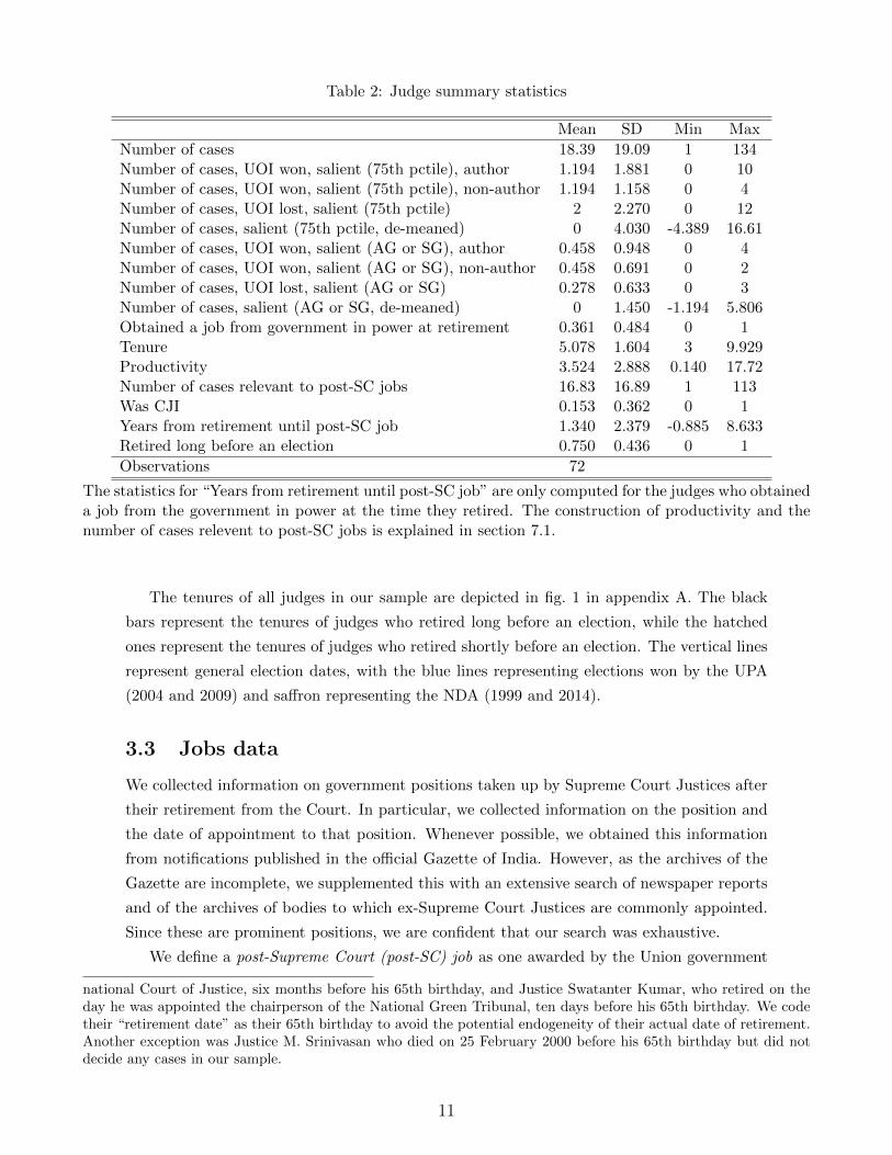
Table 2: Judge summary statistics

Mean SD Min Max

Number of cases 18.39 19.09 1 134Number of cases, UOI won, salient (75th pctile), author 1.194 1.881 0 10Number of cases, UOI won, salient (75th pctile), non-author 1.194 1.158 0 4Number of cases, UOI lost, salient (75th pctile) 2 2.270 0 12Number of cases, salient (75th pctile, de-meaned) 0 4.030 -4.389 16.61Number of cases, UOI won, salient (AG or SG), author 0.458 0.948 0 4Number of cases, UOI won, salient (AG or SG), non-author 0.458 0.691 0 2Number of cases, UOI lost, salient (AG or SG) 0.278 0.633 0 3Number of cases, salient (AG or SG, de-meaned) 0 1.450 -1.194 5.806Obtained a job from government in power at retirement 0.361 0.484 0 1Tenure 5.078 1.604 3 9.929Productivity 3.524 2.888 0.140 17.72Number of cases relevant to post-SC jobs 16.83 16.89 1 113Was CJI 0.153 0.362 0 1Years from retirement until post-SC job 1.340 2.379 -0.885 8.633Retired long before an election 0.750 0.436 0 1

Observations 72

The statistics for “Years from retirement until post-SC job” are only computed for the judges who obtaineda job from the government in power at the time they retired. The construction of productivity and thenumber of cases relevent to post-SC jobs is explained in section 7.1.

The tenures of all judges in our sample are depicted in fig. 1 in appendix A. The black

bars represent the tenures of judges who retired long before an election, while the hatched

ones represent the tenures of judges who retired shortly before an election. The vertical lines

represent general election dates, with the blue lines representing elections won by the UPA

(2004 and 2009) and saffron representing the NDA (1999 and 2014).

3.3 Jobs data

We collected information on government positions taken up by Supreme Court Justices after

their retirement from the Court. In particular, we collected information on the position and

the date of appointment to that position. Whenever possible, we obtained this information

from notifications published in the official Gazette of India. However, as the archives of the

Gazette are incomplete, we supplemented this with an extensive search of newspaper reports

and of the archives of bodies to which ex-Supreme Court Justices are commonly appointed.

Since these are prominent positions, we are confident that our search was exhaustive.

We define a post-Supreme Court (post-SC) job as one awarded by the Union government

national Court of Justice, six months before his 65th birthday, and Justice Swatanter Kumar, who retired on theday he was appointed the chairperson of the National Green Tribunal, ten days before his 65th birthday. We codetheir “retirement date” as their 65th birthday to avoid the potential endogeneity of their actual date of retirement.Another exception was Justice M. Srinivasan who died on 25 February 2000 before his 65th birthday but did notdecide any cases in our sample.

11

to a retired Supreme Court Justice. Examples include Chairman or Member of the National

Human Right Commission, Competition Appellate Tribunal, Law Commission of India and

Press Council of India. We provide a full list in table 11 in appendix A. For a judge who is

appointed to several post-SC jobs over time, we consider the first job as his post-SC job, since

appointment to later jobs is likely to be affected by his performance in previous post-SC jobs

rather than pandering while being an active judge.

From time to time, the Supreme Court constitutes committees to investigate issues that

arise in specific cases and appoints ex-SC judges to these committees. We exclude these

jobs since they are not awarded by the executive and are therefore unrelated to the type of

corruption we investigate here. The summary statistics for judge level variables are reported

in table 2.

4 Empirical strategy

We focus on corruption in the form of pandering, i.e., judges manipulating decisions in salient

cases in favour of the government in order to increase the likelihood of obtaining a post-SC

job. At the case level, pandering occurs if the judges decide in favour of the government when,

based on the merits of the case, the opposite decision should have been made.22 Unfortunately,

as any assessment of the merits of a case is inherently subjective, it is practically infeasible

to use this approach to identify pandering in our sample of 662 cases.

Instead, we can statistically identify the presence of pandering by comparing benches com-

posed of judges who have stronger incentives to pander to those who have weaker incentives

to pander. We define pandering incentives as being jointly determined by

1. the salience of the case, and

2. whether the judge retires long enough before an election.

Our measure for the salience of a case is an index comprising the four following variables:

the number of 1) Attorneys General, 2) Solicitors General, 3) Senior Advocates, and 4) Ad-

vocates that appeared in the case. The Attorney and Solicitor General are the primary and

secondary lawyers of the government, respectively. Both appointments are political, with the

Attorney General being a constitutional position equivalent in rank to a cabinet minister. As

such, these lawyers only appear in cases of great importance to the government. Depending

on the importance of a case, it is possible for more than one of the above to represent the

government in the same case. These two variable therefore proxy for the value of winning the

case for the government.

The number of Senior Advocates appearing in a case is our third proxy for its salience.23

Senior Advocates are lawyers who specialise in appearing before the High Courts and the

Supreme Court and “represent the scarcest and priciest legal talent in India” (Chandra,

22We use this dichotomous definition as we only observe whether the government has won or lost a case, withoutany information on how favourable the judgement was for the government.

23Senior Advocate is the Indian designation that is equivalent to Senior Counsel in Commonwealth jurisdictionsor Queen’s Counsel in the UK.

12

Hubbard, and Kalantry 2017). The government and other litigants often hire them in cases

that are important enough to justify their high fees. Finally, we also proxy for salience using

the number of advocates appearing in a case. This reveals the importance of the case for

the litigants as it measures the amount of resources they are willing to spend on winning it.

Hence, these two variable proxy for the sum of efforts exerted by litigants in a case, and are

therefore indicative of the value the government places on winning the case.24

We compute the first principal component of these four variables, normalise it to have

zero mean and unit standard deviation and use that as the index of salience.25 The summary

statistics for these four variables and their factor loadings in the index are presented in table 1.

We expect that pandering, if it exists, will manifest itself in cases with high salience.

Whether a judge retired long before an election or not is captured by whether the judge

retired from the Supreme Court at least 16 months (1.34 years) before an election. We

choose this threshold because, as seen in the summary statistics presented in table 2, it takes

on average about 16 months to secure a post-SC job from the government, conditional on

securing it at all. Judges who retire less than 16 moths before the next election have much

weaker incentives to pander to the government in power at the time of their retirement, as

they are unsure about whether that government will still be in power after the election. In

section 7, we show that judges who retired at least 16 months before an election are indeed

more likely to obtain a post-SC job from the government in power at the time of retirement.

To transform this variable into pandering incentives at the bench level, we simply construct

two dummy variables that indicate whether the bench is composed of one or both judges

retiring long before an election. The omitted category is composed of the benches in the

“control group” with neither of the two judges retiring long before an election. In section 5.2.6

we show that our results are robust to alternative specifications for this variable.

As described in section 2.2 and section 3.2, the date of retirement of judges is mechanically

determined by their date of birth, and furthermore, elections occurred at regular five-year

intervals. Hence, whether a judge is going to retire long before an election is predictable while

he is deciding cases and, moreover, exogenous. Consequently the number of judges on the

bench who retire long before an election is also exogenous.

We identify pandering using difference-in-differences, where the two dimensions of varia-

tion are the salience of a case and whether judges retired long before an election. We can think

of benches with two judges retiring long before an election as the “high treatment group”,

those with just one judge retiring long before an election as the “low treatment group” and

those with both retiring shortly before an election as the “control group”. We compare the

salient–non-salient difference in decisions between the two treatment groups and the control

24Because of limitations in our data, our measure is the total number of advocates (senior and non-senior) forthe government and all other litigants, rather the ideal measure of the number of advocates appearing for thegovernment only. Nevertheless, the number of advocates appearing for the government is very likely to be highlycorrelated with the total number of advocates for all parties. Hence, our measure is a reasonable proxy for theimportance of a case.

25We show the robustness of our results to using the proxies separately in table 14 in appendix B. These resultsare discussed in section 5.2.3.

13

group to obtain our estimates of the effect of pandering incentives. Our identifying assump-

tion is that the difference in the merits between salient and non-salient cases does not vary

based on the composition of the bench deciding the cases, in particular, based on how many

judges on the bench retire long before an election. This assumption is predicated on the

practice of random allocation of cases to benches described in 2.1.

The basic idea behind the identification strategy is illustrated by the simple three-by-two

bar chart in fig. 2 in appendix B. The three bars in the left-hand panel show the propor-

tion of non-salient cases (bottom 75% in terms of the salience index) decided in favour of

the government by benches with zero, one, and two judges retiring long before an election

respectively. The three bars in the right-hand panel show the same proportions for salient

cases (top 25% in terms of salience index). We see that the difference in the likelihood of the

government winning a salient relative to a non-salient case increases as the number of judges

on the bench that retire long before an election increases.

4.1 Random allocation of cases

The key to our identification strategy stated above is that the two-judge bench cases, which

constitute our sample, were randomly allocated to benches. As stated in section 2.1, this

is the Supreme Court’s stated policy and is confirmed by practitioners. Nevertheless, one

may be concerned that benches were allocated in a non-random way for some cases in our

sample. Although we cannot test the assumption of random allocation of cases directly, we

can investigate whether observed covariates differ by the number of judges retiring long before

an election. The results of tests of such differences are reported in table 3.

Most observed case characteristics do not appear to vary monotonically as the number of

judges retiring long before an election increases. However, there are some differences. For

example, we find that the the number of cases where the government is the respondent (rather

than the appellant or petitioner), appears to increase as the number of judges retiring long

before an election increases. To account for these differences, we control for these variables in

all our regressions. Finally, in section 5.2.2 we test the robustness of our results to controlling

for interactions of these variables with salience or retirement characteristics.

We also find that some components of salience, and the overall index vary with the re-

tirement characteristics of the bench. This correlation is robust to controlling for other case

characteristics and year dummies as seen in table 12 in appendix B. Since parties may choose

their litigation effort after the case is allocated to a bench, a relationship between retirement

characteristics and salience is not surprising as we discuss in section 5.3.4.

5 Pandering incentives and judicial decisions

In this section, we present our main results about the presence of pandering. We also test

them for robustness and address potential concerns about bias. To estimate the average effect

14

Table 3: Sample balance

(1) (2) (3) (4) (5) (6)0 1 2 1–0 2–0 2–1

Appeal (1) Petition (0) 0.901∗∗∗ 0.825∗∗ 0.838∗∗ -0.0761∗ -0.0626 0.0135(0.300) (0.381) (0.369) (0.0438) (0.0425) (0.0314)

UOI appellant/petitioner (1) Respondent (0) 0.527 0.421 0.344 -0.106∗ -0.184∗∗∗ -0.0778∗

(0.502) (0.495) (0.476) (0.0599) (0.0579) (0.0406)

CJI present in case 0.0110 0.0250 0.0137 0.0140 0.00276 -0.0113(0.105) (0.156) (0.117) (0.0176) (0.0137) (0.0115)

Senior judge’s tenure at case decision date 4.727∗∗∗ 4.508∗∗∗ 4.305∗∗∗ -0.219 -0.422∗∗∗ -0.202∗

(1.146) (1.326) (1.297) (0.155) (0.152) (0.110)

Junior judge’s tenure at case decision date 1.353 1.755∗ 1.290 0.402∗∗∗ -0.0635 -0.465∗∗∗

(0.916) (1.003) (0.815) (0.119) (0.101) (0.0764)

Years from decision to election 2.281∗∗ 2.173 2.545∗ -0.107 0.265 0.372∗∗∗

(1.123) (1.337) (1.406) (0.155) (0.162) (0.115)

Number of Attorneys General 0 0.0286 0.0275 0.0286 0.0275 -0.00108(0) (0.167) (0.164) (0.0175) (0.0172) (0.0138)

Number of Solicitors General 0 0.0536 0.0412 0.0536∗∗ 0.0412∗∗ -0.0123(0) (0.226) (0.199) (0.0237) (0.0209) (0.0178)

Number of Senior Advocates 0.868 1.482 1.505 0.614∗∗∗ 0.637∗∗∗ 0.0230(0.957) (2.070) (1.938) (0.225) (0.211) (0.168)

Number of Advocates 9.330 11.90 11.54 2.567 2.213 -0.353(10.86) (17.45) (14.51) (1.942) (1.650) (1.341)

Salience -0.282 0.0548 0.0353 0.336∗∗∗ 0.317∗∗∗ -0.0195(0.511) (1.138) (0.962) (0.123) (0.105) (0.0881)

Observations 91 280 291 371 382 571

Columns (1)–(3) report the means of the variables for benches with zero, one and two judges retiringlong before an election. Columns (4)–(5) report the difference between such benches. Standard errors inparentheses. ∗ p < 0.1, ∗∗ p < 0.05, ∗∗∗ p < 0.01

15

of incentives on judicial decisions we begin with the specification

wonikt = α0 +∑

jαjbjk + δt + β saliencei

+ λ1 saliencei × one retired long beforek

+ λ2 saliencei × both retired long beforek + X′ikη + εikt (1)

where wonik is an indicator for whether the Union government won case i decided by bench k.

The indicators bjk capture whether judge j was part of bench k, so that∑

jαjbjk are essen-

tially judge dummies. There are two judge dummies that are active in every case since each

case in our sample is decided by a bench composed of two judges.

The variables on the right-hand side of eq. (1) capture pandering incentives, while the

dependent variable captures the behaviour induced by them. The key parameters of interest

are λ1 and λ2. Since our salience index is normalised to have mean zero and standard

deviation one, λ1 measures the increase in the likelihood of a salient case, i.e., a case that is

one standard deviation above the mean, being decided in favour of the government when it is

decided by a bench with one judge retiring long before rather than a bench with both judges

retiring shortly before an election; similarly, λ2 measures the difference between benches with

both judges retiring long before and both retiring shortly before an election. We interpret

positive and significant estimates of λ1 and λ2 as evidence of the behavioural response to

pandering incentives.

The matrix Xik consists of case and bench characteristics, namely whether the case was an

appeal or fresh petition, whether the government was the appellant/petitioner or respondent,

the tenures of the two judges on the bench, and whether the CJI was one of the judges on the

bench. δt are year dummies. Note that in any specification that includes judge dummies we

cannot estimate the effect of one and both judges retiring long before since these two variables

are a sum of the two judge-specific dummies that indicate whether each judge retires long

before the election, so that they are fully determined by the judge dummies.

5.1 Main results

The results from regressing our main specification (1) using OLS are reported in table 4. We

cluster the standard errors at the judge dyad level to account for possible correlation of the

error term across cases decided by the same judge.26 We observe that the estimates of the

key parameters λ1 and λ2 are positive, stable and significant in all specifications, indicating

that judges do engage in corruption by favouring the government when the case is salient and

the judges retire long before an election.

To establish the presence of pandering, that is, to show that there is a causal effect

of incentives on judicial decisions, we need to rule out the possibility that our results are

26To implement dyad-robust clustering proposed in Cameron and Miller (2014), we wrote a Stata code thatis available upon request. This form of clustering subsumes both two-way clustering by judge and bench levelclustering. We discuss this in appendix D.

16

Table 4: Effect of pandering incentives on decisions.

(1) (2) (3) (4) (5)

Salience -0.387∗∗∗ -0.369∗∗∗ -0.373∗∗∗ -0.288∗∗∗ -0.285∗∗∗

(0.0509) (0.0604) (0.0649) (0.0420) (0.0429)

One retired long before 0.0597 0.0815 0.0658(0.0409) (0.0561) (0.0713)

Both retired long before 0.0153 0.0364 0.0259(0.0722) (0.0733) (0.0951)

One retired long before 0.336∗∗∗ 0.326∗∗∗ 0.328∗∗∗ 0.248∗∗∗ 0.244∗∗∗

× Salience (0.0656) (0.0745) (0.0807) (0.0584) (0.0586)

Both retired long before 0.438∗∗∗ 0.425∗∗∗ 0.425∗∗∗ 0.342∗∗∗ 0.341∗∗∗

× Salience (0.0543) (0.0619) (0.0696) (0.0669) (0.0673)

Case controls No Yes Yes Yes Yes

Year dummies No No Yes No Yes

Judge dummies No No No Yes Yes

Observations 662 662 662 662 662R2 0.036 0.061 0.076 0.222 0.236Mean of dep. var. 0.540 0.521 0.533 0.575 0.575p-value H0 : λ1 = λ2 0.000 0.000 0.000 0.007 0.003p-value H1

0 : β + λ1 = 0 0.022 0.032 0.060 0.217 0.224p-value H2

0 : β + λ2 = 0 0.037 0.014 0.026 0.142 0.144

Dependent variable is whether government won. Case controls are type of case (appeal/petition), whethergovernment was appellant/petitioner, whether CJI was one of the judges, the tenures of the senior andjunior judge at the time of decision. The mean of the dependent variable is the probability that thegovernment wins a case with mean salience when it is decided by a control group bench. Standard errorsreported in the parentheses are clustered at the judge dyad level. ∗ p < 0.1, ∗∗ p < 0.05, ∗∗∗ p < 0.01

17

driven by ideological alignment of judges with political parties. For example, judges who

are ideologically aligned with the ruling party could be more likely to decide in favour of

the government. Although undesirable, we do not consider this pandering. Instead, we

define pandering as behaviour that arises in response to extrinsic incentives rather than

intrinsic motivations such as ideology or innate characteristics. Ideological alignment or

other unobservable time-invariant judge characteristics are unlikely to introduce bias in our

regressions because they are unlikely to be correlated with our regressors. First, as discussed

in section 2.1, the allocation of cases to judges is random, so that whether a judge is assigned

a salient case or not is uncorrelated with his personal characteristics. Second, whether a

judge retires long before an election or not is decided solely by his date of birth and the date

of the next election, both of which are exogenous.27

Nonetheless, to rule out the possibility of any bias caused by unobservable judge charac-

teristics, we include judge dummies in eq. (1). These results are reported in columns (4)–(5).

The estimates of the key parameters of interest λ1 and λ2, continue to be positive and signifi-

cant. Note that the presence of judge dummies does not rule out all type-based explanations

of our results. It is possible that not all judges respond to pandering incentives. In particular,

perhaps only a subset of judges retiring long before an election who are corruptible actually

respond to pandering incentives by deciding in favour of the government. This would imply

that there are heterogeneous effects of pandering incentives and that we are estimating the

average treatment effect.

Furthermore, to control for time-specific effects, we also include dummies for the year in

which the case was decided. These absorb any changes in the decisions induced by political

and institutional changes over time, for e.g., the increase in the number of judges in 2008. In

section 5.2.2 we show the robustness of our results to including other interactions to check

whether our results are driven by, for example, changes in how judges decide salient cases

over their tenure.

The estimated values for the interaction term from columns (1)–(5) indicate that for a

case that is one standard deviation higher than the mean in salience, the probability of the

government winning is about 24 to 27 percentage points higher when the case is decided by a

bench with one judge retiring long before an election relative to a bench composed of judges

both of whom retire shortly before an election. Similarly, the likelihood of the same case

being decided in favour of the government is 30 to 36 percentage points higher when the case

is decided by a bench with both judges retiring long before an election relative to both judges

retiring shortly before.

We also test the hypothesis that pandering increases as the number of judges retiring

long before an election increases from one to two. The hypothesis that λ1 = λ2 is rejected

at 1% in all specifications suggesting that the effect of pandering incentives is monotonically

increasing in the number of judges retiring long before an election. We discuss the tests of

27The three elections that took place within our sample period occurred regularly once every five years: 2004,2009, and 2014.

18

H10 and H2

0 in section 5.3.4.

Based on the mean of the dependent variable and the effect of salience we observe that

the government has a 23–31% chance of winning a case that is one standard deviation higher

than mean salience that is decided by a bench with both judges retiring shortly before an

election. Our estimates imply that the probability of the government winning such a case

more than doubles when it is instead decided by a bench with both judges retiring long before

an election.

In addition to λ1 and λ2, the estimates for β, the coefficient on salience, are significant in

all specifications. This suggests that cases with higher salience are less likely to be decided

in favour of the government by control group benches. This is also observed in fig. 2 in

appendix B where the likelihood of salient cases being decided in favour of the government

by the control group is markedly lower. There are three possible explanations for this.

First, it is possible that all benches pander in non-salient cases, but only the treatment

benches pander in the salient ones. This is plausible since there is greater public scrutiny

of salient cases and blatant pandering in such cases, particularly in the presence of senior

lawyers, is less likely. Hence, only judges with strong pandering incentives would pander in

salient cases, where the rewards make up for the added reputational risk induced by increased

scrutiny. This would raise the likelihood of non-salient cases being decided in favour of the

government by control benches relative to salient ones, and yield a negative estimate of β.

If true, this would mean we are underestimating pandering since our identification strategy

differences out any pandering that occurs in non-salient cases by all judges. Second, it is

possible that salience is negatively correlated with merits so that the negative estimates of

β indicate that, on merits, more salient cases are less likely to be decided in favour of the

government. Our identification strategy accommodates this since we only assume that the

difference in merits between salient and non-salient cases is uncorrelated to the allocation of

cases to benches. Finally, the negative estimates of β may suggest that lacking incentives to

pander, control group judges actively decide against the government in more salient cases with

a view to grandstand and present themselves as being independent of government control.

We consider this possibility in section 6.2.

5.2 Robustness

In this section, we test the robustness of our results to perturbing different elements of the

baseline specification.

5.2.1 Disaggregated effects of election-retirement distance

The regression specification in (1) assumes that pandering incentives are active when a judge

retires more than 16 months before the next election and inactive otherwise. It is possible

however that even among judges retiring more than 16 months before the next election,

pandering incentives vary based on how long before the next election they retire. In this

19

section, we estimate the heterogenous effect of pandering incentives separately for benches

based on which of the four 16 month periods before the next election the judges retire. Since

there are two judges in each bench and they can retire in one of four such periods, there are

10 possible combinations which we call retirement categories. We therefore estimate

wonikt = α0 +∑

jαjbjk + δt + β saliencei+

+9∑

`=1

λ` (saliencei × retirement category`k) + X′iη + εikt , (2)

where retirement category`k is a dummy taking value 1 if the judges in bench k belong to

retirement category ` and 0 otherwise. Our base is retirement category 0 which corresponds

to both judges retiring shortly (0–1 years) before an election. The correspondence between

the other categories and the number of judges retiring in each year is shown in table 13 in

appendix B, together with the estimates of λ`.

We can interpret the coefficient estimate for an interaction term, for example λ3, as the

change in the probability that the government wins a salient case (that is, a case with one

standard deviation higher than mean salience) when we replace one judge from a bench with

both judges retiring close to an election such that one retires between 32–48 months before

the next election.

All the estimates of λ` are positive and almost all are significant at 1% indicating that all

benches pander more than benches where both judges retire shortly before an election.

Finally, we also test the robustness of our results to perturbing the threshold for when

a judge is considered to have retired long before an election. In particular, our results are

robust to choosing thresholds of 6, 12, 18 and 24 months as shown in table 16 in appendix B.

We note that the estimates of λ1 and λ2 in columns (4) and (8) for a threshold of 2 years are

markedly smaller in magnitude than the corresponding ones in the main results. This is as

expected, since many judges in the treatment groups are now included in the control group,

thereby attenuating the difference in behaviour between the groups.

5.2.2 Controlling for other interactions

One concern with our results is that the interaction terms that capture pandering incentives

are potentially proxying for some other variables that affect the outcome of the case. In

particular, we saw in table 3 that some case characteristics were significantly different between

the treatment and control groups. Although we include case controls in our regressions,

it is possible that the true effect of these controls on decisions is through an interaction

with salience or retirement distance. In this section, we address this concern by separately

interacting the controls that were significantly different across our “treatment” and “control”

groups with the two variables that together make up pandering incentives.

The results are presented in table 5. In the first column, we present our baseline results for

comparison. In column (2) we consider whether the two treatment groups rule cases differently

20

when UOI is appellant/petitioner relative to when UOI is the respondent. Similarly, in

column (3) we control for the interaction of salience with the role of the UOI. In columns (4)

and (5) we do the same with the years between the decision date of the case and the next

election date. Finally, in columns (6) and (7) we repeat this exercise with the length of the

tenure of the junior judge at the time of the decision.

We observe that the coefficients on pandering incentives continue to be robust to the

inclusion of these interactions, and the coefficient estimates in table 5 are very similar in

magnitude to our baseline specification reported in the first column, suggesting that the

results are unlikely to be driven by the interaction of treatment benches or salience with

other case characteristics.

5.2.3 Different proxies for salience

In this section, we test the robustness of the results with respect to varying the proxy for

salience. So far, we have used the normalised first principal component of the four different

proxies presented in section 4 as our index for salience.

We first present results using the different proxies that make up our salience index. Results

are reported in table 14 in appendix B. To begin with, we use the presence of Attorney or

Solicitor General as a proxy for salience.28 We see in columns (1) and (2) that the estimates

for the interaction term are positive.

In columns (3) and (4), we use the number of Senior Advocates appearing in the case as a

proxy for its salience. In columns (5) and (6) we use the number of advocates, that is, junior

advocates with no special designation, as our proxy for salience. We observe that the estimates

for the interaction terms remain positive and mostly significant across these specifications.

We observe that the results are qualitatively similar regardless of the particular proxy used.

These results support our strategy of collapsing these four variables into one index using the

first principal component.

So far we have assumed that pandering incentives increase linearly with salience. Next,

we disaggregate our salience measure into quartiles and we report the results in table 15

in appendix B. The lowest quartile of cases by salience forms the omitted category. We

observe that the estimates of the interaction terms increase in magnitude with the quartiles

of salience, being significant for the highest quartiles.

5.2.4 Cases with no clear winner

In our data collection interface, we gave three options for coding the outcome of a case:

government won, government lost, and winner not identifiable. The last option was to allow

for cases where it was not clear if the government won or lost. This could happen when, for

example, some of the points in dispute in a case were decided in favour of the government but

28We use the presence of either Attorney or Solicitor General as there are only 17 cases in our sample where onlythe Attorney General appears.

21

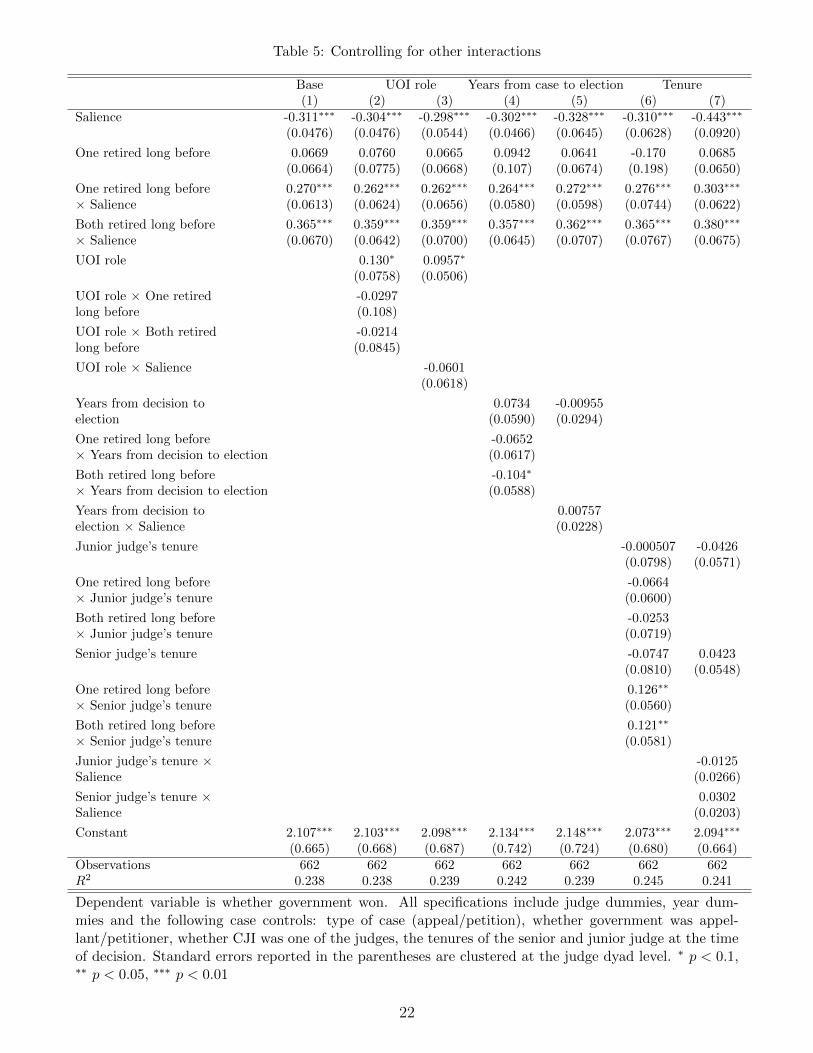
Table 5: Controlling for other interactions

Base UOI role Years from case to election Tenure(1) (2) (3) (4) (5) (6) (7)

Salience -0.311∗∗∗ -0.304∗∗∗ -0.298∗∗∗ -0.302∗∗∗ -0.328∗∗∗ -0.310∗∗∗ -0.443∗∗∗

(0.0476) (0.0476) (0.0544) (0.0466) (0.0645) (0.0628) (0.0920)

One retired long before 0.0669 0.0760 0.0665 0.0942 0.0641 -0.170 0.0685(0.0664) (0.0775) (0.0668) (0.107) (0.0674) (0.198) (0.0650)

One retired long before 0.270∗∗∗ 0.262∗∗∗ 0.262∗∗∗ 0.264∗∗∗ 0.272∗∗∗ 0.276∗∗∗ 0.303∗∗∗

× Salience (0.0613) (0.0624) (0.0656) (0.0580) (0.0598) (0.0744) (0.0622)

Both retired long before 0.365∗∗∗ 0.359∗∗∗ 0.359∗∗∗ 0.357∗∗∗ 0.362∗∗∗ 0.365∗∗∗ 0.380∗∗∗

× Salience (0.0670) (0.0642) (0.0700) (0.0645) (0.0707) (0.0767) (0.0675)

UOI role 0.130∗ 0.0957∗

(0.0758) (0.0506)

UOI role × One retired -0.0297long before (0.108)

UOI role × Both retired -0.0214long before (0.0845)

UOI role × Salience -0.0601(0.0618)

Years from decision to 0.0734 -0.00955election (0.0590) (0.0294)

One retired long before -0.0652× Years from decision to election (0.0617)

Both retired long before -0.104∗

× Years from decision to election (0.0588)

Years from decision to 0.00757election × Salience (0.0228)

Junior judge’s tenure -0.000507 -0.0426(0.0798) (0.0571)

One retired long before -0.0664× Junior judge’s tenure (0.0600)

Both retired long before -0.0253× Junior judge’s tenure (0.0719)

Senior judge’s tenure -0.0747 0.0423(0.0810) (0.0548)

One retired long before 0.126∗∗

× Senior judge’s tenure (0.0560)

Both retired long before 0.121∗∗

× Senior judge’s tenure (0.0581)

Junior judge’s tenure × -0.0125Salience (0.0266)

Senior judge’s tenure × 0.0302Salience (0.0203)

Constant 2.107∗∗∗ 2.103∗∗∗ 2.098∗∗∗ 2.134∗∗∗ 2.148∗∗∗ 2.073∗∗∗ 2.094∗∗∗

(0.665) (0.668) (0.687) (0.742) (0.724) (0.680) (0.664)Observations 662 662 662 662 662 662 662R2 0.238 0.238 0.239 0.242 0.239 0.245 0.241

Dependent variable is whether government won. All specifications include judge dummies, year dum-mies and the following case controls: type of case (appeal/petition), whether government was appel-lant/petitioner, whether CJI was one of the judges, the tenures of the senior and junior judge at the timeof decision. Standard errors reported in the parentheses are clustered at the judge dyad level. ∗ p < 0.1,∗∗ p < 0.05, ∗∗∗ p < 0.01

22

others were decided against the government. There were only 20 cases where the outcome of

a case was coded as not identifiable, and as described in section 3.1, these were dropped from

our analysis.

We now include these 20 cases and code them in different ways to see whether our results

are robust to their inclusion. Results are reported in table 17 in appendix B. In columns

(1) and (2) we include these cases among the ones that the government lost. In columns

(3) and (4) we do the opposite and include these cases among the ones that the government

won. Finally in columns (5) and (6), to allow for the possibility that the decision in these

cases was partly in favour of the government and partly against it, we construct a dependent

variable that takes value 1 for the cases where the government won, -1 for the cases where the

government lost, and 0 for these 20 cases where the winner was not identifiable. The estimates

of our coefficients of interest remain positive indicating that the inability to determine clearly

whether the government won or lost in a subset of cases does not affect our results.

5.2.5 Alternative functional forms

So far we have used the linear probability model. Next we rerun our baseline specification

using logit and probit instead. We observe that the coefficient estimates of λ1 and λ2 remain

positive and significant. The results are reported in table 18 in appendix B.

5.2.6 Constant marginal effects and average treatment effects

In all the specifications so far, we used factor variables to indicate the three kinds of benches,

that is, those with zero, one, or two judges retiring long before an election. In this section

we consider two restrictions.

First, we run a restricted version of eq. (1) by imposing linearity on the effect of pandering

incentives in the number of judges retiring long before an election. We estimate

wonikt = α0 + β saliencei +∑

jαjbjk + δt

+ λ saliencei × num retired long beforek + X′ikη + εikt. (3)

This specification uses the number of judges retiring long before an election as the interacting

variable with salience. This variable takes values 0, 1, and 2. We find that the estimates for

λ are positive, significant, and stable across all specifications.

The results of estimating eq. (3) are shown in table 19 in appendix B. The specification

in eq. (3) imposes the restriction on eq. (1) that the marginal effect of the number of judges

retiring long before an election is constant, that is λ2 = 2λ1. This restriction is rejected by

an F -test, whose p-values are reported in the last row of table 19.

23

Second, we also run

wonikt = α0 + β saliencei + λ saliencei × at least one retired long beforek

+ γat least one retired long beforek +∑

jαjbjk + δt + X′ikη + εikt . (4)

The results are reported in table 20 in appendix B. This specification pools the benches with

one or two judges retiring long before an election. This is a special case of eq. (1) as it forces

the restriction λ2 = λ1. All our results are robust to using this as our baseline specification.

However, we use eq. (1) as our baseline since the restriction above is not supported empirically,

as shown by the p-values for the F -test of this restriction reported in table 4.

5.3 Potential sources of bias

We now discuss possible sources of bias in our results. We show that these sources either

lead to no bias or a downward bias in our estimates. As such, the estimates we presented are

lower bounds of the effect of pandering incentives on judicial decisions.

5.3.1 Incentives for the “control” group

It is possible that the “control” benches, that is, benches where both judges retire shortly

before an election, have some rather than no incentives to pander. In that case, the compar-

ison between “treatment” and “control” benches is not a comparison between benches with

and without incentives, but rather a comparison between benches with stronger and weaker

incentives to pander. Therefore, our estimates of this difference are lower bounds on the true

effect of pandering incentives on judicial decisions.

5.3.2 Settlement of cases

A key concern with the literature on published judgements is selection bias – judgements may

not be a representative sample of all cases since a significant fraction of cases are actually

settled before they are decided by the court. In fact, there may be differences in the likelihood

of out-of-court settlement between cases assigned to “treatment” and “control” benches.

This point is discussed extensively in Ashenfelter, Eisenberg, and Schwab (1995), who point

out that random allocation of cases to judges means that any differences in the probability

of the government winning a case must be due to differences in judicial behaviour rather

than unobservable case characteristics. As such, the observed differences reflect the effect of

pandering incentives on judicial decisions.

5.3.3 Beliefs about elections

It is possible that pandering incentives are affected by a judge’s beliefs about elections. For

example, a judge retiring shortly before an election may pander if he believes that the gov-

ernment in power will be re-elected and he would be rewarded after the election. It is also

24

possible that a judge retiring long before an election only begins to pander after the last elec-

tion before his retirement. Another possibility is that judges may not expect the government

to last five years. Consequently, even the judges in the treatment group may not believe that

there is sufficient time left for the government at the time of their retirement to reward them

with jobs. Although the governments in the period of our study all served their full term,

the judges at the time may not have expected this.

Note that in any of these scenarios, where a particular configuration of beliefs leads to

pandering by judges who retire shortly before an election, or leads to weaker pandering by

judges who retire long before one, there will be downward bias in the difference-in-differences

estimator. The reason why the effect of pandering incentives will be underestimated is that

for at least some part of their tenure there will be little difference between the judges in our

“treatment” and “control” benches, i.e., judges who retire long and shortly before an election,

in their pandering incentives.29

Another possibility is that judges retiring shortly before an election systematically decide

salient cases against the government in power at the time of retirement. This could happen if

these judges believe that the government at the time of retirement will lose the next election

and the opposition party at the time of retirement would reward them once they form the

next government. Note that such behaviour is nonetheless an effect of pandering incentives

on judicial decision-making, albeit one where the judges retiring shortly before an election

pander to a potential future government rather than the current one.

To be precise, our estimates are based on the following two assumptions: 1) judges who

retire long before an election pander to the government in power at the time of their retirement

in all cases they decide on throughout their tenure, even before that government’s term; 2)

judges who retire shortly before an election do not pander to the government in power at the

time of their retirement in all cases they decide on throughout their tenure, even before that

government’s term. Any deviation from these assumptions, e.g., if a judge in the treatment

bench sometimes does not pander to the government in power at the time of his retirement

or a judge in the control bench sometimes does, will lead to an attenuation of the difference

between treatment and control benches. Therefore, the effect of pandering incentives are

bounded below by the positive and significant estimates in table 4.

Nonetheless, to see whether judges retiring long before an election pander more when they

are close to retirement, we interact pandering incentives with the number of judges retiring

long before who are in their final government’s term. A positive coefficient would indicate

that pandering by judges retiring long before an election intensifies when these judges reach

the term of the government in which they retire. Results reported in table 6 suggest that

this is not the case. These results indicate that judges retiring long before an election pander

uniformly throughout their tenure even before the term of the final government in power at

the time of their retirement.

29This downward bias is even stronger in the unlikely event that judges who retire shortly before an election havestronger pandering incentives than those retiring long before, as this would lead to a negative estimate of the effect.

25

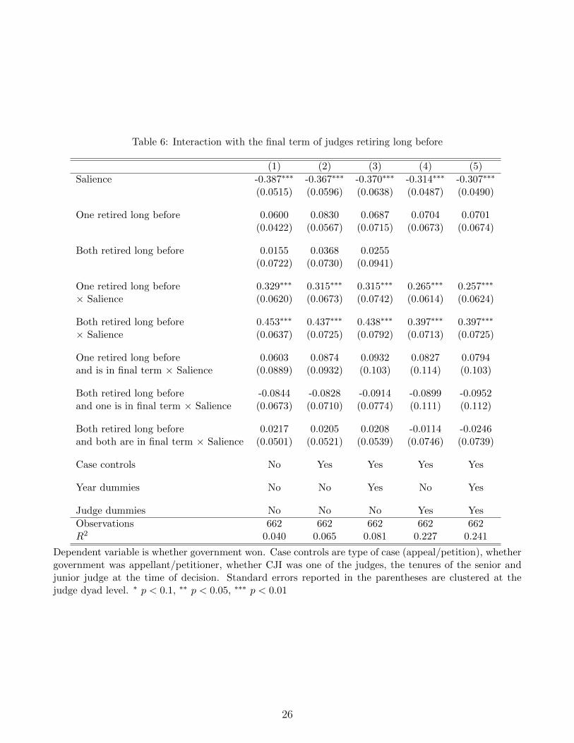
Table 6: Interaction with the final term of judges retiring long before

(1) (2) (3) (4) (5)

Salience -0.387∗∗∗ -0.367∗∗∗ -0.370∗∗∗ -0.314∗∗∗ -0.307∗∗∗

(0.0515) (0.0596) (0.0638) (0.0487) (0.0490)

One retired long before 0.0600 0.0830 0.0687 0.0704 0.0701(0.0422) (0.0567) (0.0715) (0.0673) (0.0674)



× Salience (0.0620) (0.0673) (0.0742) (0.0614) (0.0624)


× Salience (0.0637) (0.0725) (0.0792) (0.0713) (0.0725)

One retired long before 0.0603 0.0874 0.0932 0.0827 0.0794and is in final term × Salience (0.0889) (0.0932) (0.103) (0.114) (0.103)

Both retired long before -0.0844 -0.0828 -0.0914 -0.0899 -0.0952and one is in final term × Salience (0.0673) (0.0710) (0.0774) (0.111) (0.112)

Both retired long before 0.0217 0.0205 0.0208 -0.0114 -0.0246and both are in final term × Salience (0.0501) (0.0521) (0.0539) (0.0746) (0.0739)




Observations 662 662 662 662 662R2 0.040 0.065 0.081 0.227 0.241

Dependent variable is whether government won. Case controls are type of case (appeal/petition), whethergovernment was appellant/petitioner, whether CJI was one of the judges, the tenures of the senior andjunior judge at the time of decision. Standard errors reported in the parentheses are clustered at thejudge dyad level. ∗ p < 0.1, ∗∗ p < 0.05, ∗∗∗ p < 0.01

26

The government term preceding the final term for most judges in our sample is either that

of the NDA government that was in power from 1999–2004 or the UPA government that was

in power between 2004–2009. Both these governments were widely expected to be re-elected

although the former was not. Consider the behaviour of two judges, one retiring long before

and the other retiring shortly before an election. Let their tenures have the same starting

point and overlap with the terms of two governments. The results presented in table 6 are

consistent with the belief that the government preceding the final government will be re-

elected for one additional term. Under such beliefs, the judge retiring long before an election

would pander to both the government in power at the start of his tenure and the one that

follows. Similarly, a judge retiring shortly before an election will have weaker incentives to

pander to both the governments that are in power during his tenure. This is one plausible

configuration of beliefs that fits the behaviour we observe.

5.3.4 Endogenous litigant response

We have seen that treatment group benches tend to favour the government in salient cases.

This leads to the question of whether litigants are aware of this and alter their behaviour in

response. The government may choose litigation effort after observing the characteristics of

the bench deciding the case. Consequently, it is possible that the government invests more in

cases that are allocated to benches with more judges retiring long before since such benches

are more receptive to such effort. We note that table 3 indicates that the salience index is

higher for cases decided by the two treatment groups. Table 12 in appendix B shows that this

difference continues to be statistically significant even after controlling for case characteristics

and year dummies.

In the presence of such a response, our salience index captures ex-post salience, i.e., the

effort exerted by the government which ultimately may be determined by the retirement

characteristics of the bench and ex-ante salient, i.e., the value of the case to the government.

We can represent this relationship as

salienceik = ζ1one retired long beforek + ζ2both retired long beforek

+ ξ1 vi × one retired long beforek + ξ2 vi × both retired long beforek + vi, (5)

where salienceik is ex-post salience measured by our salience index and vi is ex-ante salience.

In our data, we observe salienceik while vi is unobservable. The equation allows for the

possibility that the government exerts more effort not only when vi is high but also when the

judges deciding the case retire long before an election.

In appendix C, we show that the difference in differences effects with respect to ex-ante

salience and bench retirement characteristics are

∂wonikt

∂vi|r=1 −

∂wonikt

∂vi|r=0 = ξ1(β + λ1) + λ1 (6)

27

and∂wonikt

∂vi|r=2 −

∂wonikt

∂vi|r=0 = ξ2(β + λ2) + λ2, (7)

where r ∈ {0, 1, 2} is the number of judges retiring long before.

Firstly, we note that ξ1 = ξ2 = 0 would lead to identical estimates of pandering based

on ex-post or ex-ante salience. In this special case, there is no interaction between ex-

ante salience and bench retirement characteristics in the determination of ex-post salience.

However, if the government invests additional effort when the ex-ante salience is high and

the judges retire long before, then we would have ξ1, ξ2 6= 0.

In table 4 we test the null hypotheses H10 : β+λ1 = 0 and H2

0 : β+λ2 = 0. We fail to reject

H10 and H2

0 at 10% when we include judge dummies. Consequently, in the full specifications

with judge dummies, the difference in differences effects in eq. (6) and eq. (7) simplify to

λ1 and λ2, respectively. Hence, because of the estimated magnitudes of λ1, λ2, and β in our

setting, our estimates of pandering behaviour apply not only to ex-post salience but also to

ex-ante salience. The fact that we reject H10 and H2

0 when we don’t include judge dummies

leaves open the possibility that pandering based on ex-ante salience may be larger or smaller

than based on ex-post salience depending on the sign of ξ1 or ξ2.

Our baseline results can be seen as an answer to the question of how much the probability

of the government winning an ex-post salient case changes when the case is decided by a bench

with more rather than fewer judges retiring long before. In this section, we have attempted to

answer a somewhat different question – how much does the probability that the government

wins an ex-ante salient case change when it is decided by a bench with more rather than fewer

judges retiring long before? Based on a simple model of how ex-post salience changes with

ex-ante salience and bench retirement characteristics, we have shown that our estimates in

the full specifications imply that the answer to these two questions turns out to be the same.

6 Pandering: A closer look

In this section, we examine pandering more closely and explore the channels through which

pandering occurs. In particular, we investigate four things. First, in section 6.1, we examine

how pandering manifests itself through writing favourable judgements rather than simply

being on a bench that decides in favour of the government. Second, in section 6.2 we examine

whether the lack of post-SC career incentives leads the control group judges to grandstand,

and whether this explains our results. Third, in section 6.3, we examine whether pandering

occurs through strategically delaying unfavourable decisions or expediting favourable ones.

Finally, in section 6.4 we investigate whether the effect of pandering incentives is stronger for

the senior judge on the bench, relative to the junior judge.

28

6.1 Pandering incentives and judgement authorship

The allocation of a case to a bench is randomised but the authorship of the judgement is not.

Once the two judges decide on the outcome of the case, they also jointly decide which one

of the two writes the judgement.30 The name of the judge writing the judgement is always

identified when a judgement is delivered. In this section we explore the choice of judgement

authorship to shed more light on the mechanism through which pandering occurs.

We expect that rather than simply sitting on a bench that decides in favour of the gov-

ernment, pandering may manifest itself in actually writing judgements that are favourable

to the government. There are two reasons for this. First, being the author of a favourable

judgement is more visible, and consequently more likely to be rewarded, compared to just

sitting on the bench in a case that is decided in favour of the government. Conversely, the

judge not writing the judgement is less likely to be noticed and therefore less likely to be

rewarded for favourable judgements and punished for unfavourable ones. Second, the lit-

erature on signalling shows that costly actions are an effective form of communication in

environments where talk is cheap. Since a judge’s reputation depends on the judgements

he has written, committing to written judicial reasoning for favouring the government may

be a more credible way for a judge to signal his willingness to conform to the government’s

preferences in his role after retirement in case he receives a post-SC appointment. As such

we believe that writing favourable judgement may be more important than simply deciding

in favour of the government when it comes strengthening the prospects of receiving post-SC

appointments. This hypothesis is supported by the results in section 7, where we will see

that writing favourable judgements rather than simply deciding in favour of the government

is positively associated with securing post-SC appointments.

If this is true, we expect to see a pattern in judgement writing. In particular, judges that

retire long before an election should be more likely to write judgements in cases that are

salient and where the government wins. To test this we run the following specification:

author retired long beforeikt = α+∑

jαjbjk + δt + β saliencei + γ wonik

+ λ saliencei × wonik + X′ikη + εikt. (8)

We restrict our attention to the subsample of cases where one of the judges on the bench

retired long before an election and the other retired shortly before an election. Our dependent

variable is an indicator of whether the author of the judgement retires long before an election.

If judges with pandering incentives want to be noticed by the government when they decide in

its favour in salient cases, we would expect λ to be positive. To control for the possibility that

the senior judge’s retirement-election distance may affect who writes the judgement, because

there may be a seniority norm in judgement writing, we include an indicator for whether the

30In principle both of them could write separate judgements. This rarely occurs – we only observe this happeningin 6 cases, and these are left out of our sample. In general the rarity of all judges writing separate judgements inthe same case is something of a puzzle. See Posner (2010) and Epstein, Landes, and Posner (2013) for explanationsof this phenomenon based on the ideas of effort and dissent aversion.

29

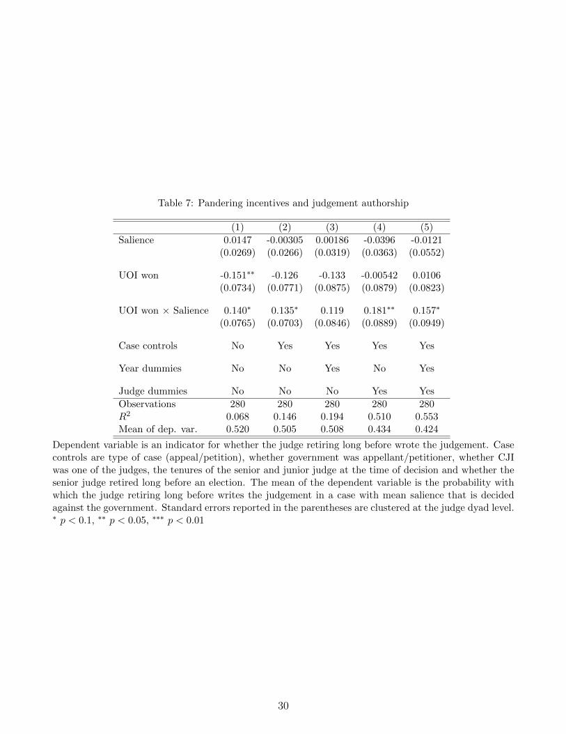
Table 7: Pandering incentives and judgement authorship

(1) (2) (3) (4) (5)

Salience 0.0147 -0.00305 0.00186 -0.0396 -0.0121(0.0269) (0.0266) (0.0319) (0.0363) (0.0552)

UOI won -0.151∗∗ -0.126 -0.133 -0.00542 0.0106(0.0734) (0.0771) (0.0875) (0.0879) (0.0823)

UOI won × Salience 0.140∗ 0.135∗ 0.119 0.181∗∗ 0.157∗

(0.0765) (0.0703) (0.0846) (0.0889) (0.0949)




Observations 280 280 280 280 280R2 0.068 0.146 0.194 0.510 0.553Mean of dep. var. 0.520 0.505 0.508 0.434 0.424

Dependent variable is an indicator for whether the judge retiring long before wrote the judgement. Casecontrols are type of case (appeal/petition), whether government was appellant/petitioner, whether CJIwas one of the judges, the tenures of the senior and junior judge at the time of decision and whether thesenior judge retired long before an election. The mean of the dependent variable is the probability withwhich the judge retiring long before writes the judgement in a case with mean salience that is decidedagainst the government. Standard errors reported in the parentheses are clustered at the judge dyad level.∗ p < 0.1, ∗∗ p < 0.05, ∗∗∗ p < 0.01

30

senior judge on the bench retires long before an election among our case controls.31

The results are reported in table 7. We observe the estimates for λ are positive across

all specifications even after controlling for case characteristics, and judge and year dummies.

Note that the sample size drops compared to our main results, as we focus on the sub-sample

of cases where one of the two judges retired long before an election and the other retired

shortly before an election. The mean of the dependent variable is close to one half in all

columns, indicating that when the case is decided against the government and is not salient,

the judge who retires long before an election is as likely to write the judgement as the judge

who retires shortly before an election. The estimates of the interaction coefficient indicate

that in salient cases that the government wins, the judgement is more likely to be authored

by the judge who retired long before an election.

It may seem that a judge-by-case-level specification, where we regress whether judge j in

case i authored the judgement on saliencei × wonik × retired long beforej would allow us to

expand our sample of cases beyond just those that were decided by one judge retiring long

before. However, since there is only one author per case, the outcome variable will always

sum to one across the two observations per case, and this induces a correlation in the error

term across the two observations in each case. More generally, pandering incentives should

only be able to explain authorship in those cases where one of the judges retires long before

and the other retires shortly before an election, since pandering incentives are equal for two

judges when they both retire long or shortly before an election.

6.2 Grandstanding

A possible alternative explanation of our results is that they reflect grandstanding by the

control group judges rather than pandering by the treatment group. It is possible that the

lack of post-SC career concerns for judges in the control group leads them to take conspic-

uous stands against the government, a behaviour which we call grandstanding. To present

themselves as being independent of government control, they may decide salient cases against

the government since these cases attract more attention from the media. On the other hand,

the treatment group judges may decide salient cases on merits. If true, this would also lead

to a positive difference-in-differences coefficient.

This explanation is consistent with post-SC career incentives having an effect on judicial

behaviour. However, if true, our results would not indicate pandering but rather grandstand-

ing. In this section, we explore this channel further. To do so, we first record the number of

news articles in the Factiva database mentioning each of the 72 judges in our sample during

their SC tenure. Our measure of grandstanding is obtained by dividing the total number of

articles for a judge by the length of his tenure.

First, we check whether grandstanding is associated with whether a judge retires long

before an election. The results are reported in table 22 in appendix A. We find that the

31As we explain in section 6.4, we cannot include an indicator for each of the senior and junior judge retiring longbefore, due to collinearity with the judge dummies.

31

Table 8: Grandstanding vs pandering

(1) (2) (3) (4) (5)

Salience -0.347∗∗∗ -0.339∗∗∗ -0.338∗∗∗ -0.235∗∗∗ -0.232∗∗∗

(0.0456) (0.0524) (0.0605) (0.0453) (0.0485)

One retired long before 0.0623 0.0833 0.0669(0.0411) (0.0559) (0.0718)



× Salience (0.0649) (0.0748) (0.0790) (0.0592) (0.0597)


× Salience (0.0510) (0.0599) (0.0669) (0.0630) (0.0641)

Normalised news articles -0.00764 -0.00872 -0.00359(0.0210) (0.0225) (0.0295)

Salience × Normalised -0.0377∗ -0.0308∗ -0.0348 -0.0550∗∗ -0.0548∗∗

news articles (0.0219) (0.0176) (0.0228) (0.0279) (0.0272)




Observations 662 662 662 662 662R2 0.039 0.062 0.078 0.225 0.239

Dependent variable is whether government won. All specifications include judge dummies, year dum-mies and the following case controls: type of case (appeal/petition), whether government was appel-lant/petitioner, whether CJI was one of the judges, the tenures of the senior and junior judge at the timeof decision. Standard errors reported in the parentheses are clustered at the judge dyad level. ∗ p < 0.1,∗∗ p < 0.05, ∗∗∗ p < 0.01

32

estimates are negative, suggesting that control group judges grandstand more on average.

However, the estimates are consistently insignificant. To investigate further, we measure

grandstanding for a bench with the sum of the individual measures for the judges on that

bench. We then run our baseline specification in eq. (4) with the addition of the interaction

of salience and grandstanding at the bench level. The results are presented in table 8.

We find that the estimates of the key coefficients of interest remain largely unchanged.

This indicates that pandering incentives, namely the interaction of salience and retirement-

election distance, are not proxying for the interaction of salience and grandstanding. Inter-

estingly, the coefficient for the new interaction term is negative and significant. This suggests

that judges that grandstand decide salient cases against the government more frequently.

Nonetheless, as mentioned earlier, this effect is independent of pandering and does not ap-

pear to be the channel through which post-SC career incentives affect judicial decisions.

6.3 Strategic delay or hastening of decisions

In this section, we examine whether there is any evidence that pandering occurs through

judges delaying unfavourable decisions and/or expediting favourable ones. A possible pander-

ing mechanism is that judges retiring long before an election pander by strategically delaying

those decisions that are unfavourable to the government. This strategic behaviour would lead

to our sample being censored, since judges retiring long before an election would delay making

unfavourable decisions in salient cases. Once they retire, such cases would then be reassigned

to other judges. This mechanism is consistent with the idea of pandering incentives having

an effect on judicial behaviour. However, it may have different welfare implications from the

channel where the actual decision in the case is affected by pandering incentives.

Unfortunately, we cannot directly observe cases that judges never decide on if the case is

delayed beyond retirement. However, we can test whether pandering incentives affect how

quickly judges decide cases that are in our sample. In our data, we observe the year in which

the case was filed in the Supreme Court. Subtracting this from the date on which the case

was decided, we can measure how long it took for the case to be decided.32 To test whether

treatment benches delay salient cases where the government loses we run

time to decisionikt = α0 +∑

jαjbjk + δt + β0 saliencei + β1wonik + β2 saliencei × wonik

+ γ1 saliencei × one retired long beforek + γ2 saliencei × both retired long beforek

+ λ1 wonik × saliencei × one retired long beforek + ψ1wonik × one retired long beforek

+ λ2 wonik × saliencei × both retired long beforek + ψ2wonik × both retired long beforek

+ X′ikη + εikt . (9)

32Unlike the exact date of decision, which we observe, we only observe the year in which the case was filed. Wetherefore treat all cases as being filed on the 1st of January of the year of filing. This measurement error in thedependent variable is likely to increase our standard errors but unlikely to introduce any bias as we do not expectcase characteristics to be systematically correlated with whether a case is filed early or late in a calendar year.

33

If treatment benches strategically delay unfavourable decisions in salient cases, we would

expect γ1 and γ2 to be positive. This would be a test of the hypothesis described above

under the assumption that treatment benches attempt to delay unfavourable decisions in

salient cases relative to control benches, and that not all such cases are delayed beyond the

retirement of the judges in the bench. The latter is a reasonable assumption since our sample

does contain salient cases that were decided against the government by treatment group

benches. The estimates for γ1 and γ2 essentially test for the presence of delay in these cases.

The results are reported in table 21 in appendix B. All estimates of γ1 and γ2 are insignif-

icant and show no pattern across the columns. Moreover, this specification also allows us to

test whether treatment benches strategically expedite decisions in salient cases that are in

favour of the government. If this occurs we would expect the estimates for λ1 and λ2 to be

negative. We find no such effect. Strategic delay or hastening of decisions does not appear

to be the channel through which pandering occurs.

6.4 Pandering incentives and seniority

A seniority norm may be at work in the Supreme Court with regard to authorship of judge-

ments. According to the norm, the senior judge on the bench has the authority to decide

who authors the judgement: the senior judge may do it himself, or assign it to his junior

on the bench. Seniority in the Supreme Court is based purely on the tenure on the Court

which, as discussed in section 2.2, is determined by the date of appointment to the Court.

In this section, we attempt to test whether there is a differential effect of the senior judge’s

pandering incentives on judicial decisions relative to that of the junior judge. We run

wonikt = α0 +∑

jαjbjk + δt + β saliencei + γS senior retired long beforek

+ λS saliencei × senior retired long beforek

+ λJ saliencei × junior retired long beforek + X′ikη + εikt . (10)

The results of estimating this specification are reported in table 23 in appendix B. Note that

in columns (4) and (5) we cannot estimate the effect of the junior judge retiring long before

an election since the sum of the dummies for senior and junior judge retiring long before are

equal to the number of judges retiring long before. This in turn is fully determined by judge

characteristics and hence perfectly collinear with the judge dummies. The estimates for λS

and λJ are positive and significant across all specifications. This suggests that the pandering

incentives of both the senior and the junior judge have an effect on the decision in the case.

The estimates for λS and λJ are similar in magnitude suggesting that there is no differential

effect of pandering incentives of the senior judge. We test for the equality of λS and λJ

and find that we cannot reject this hypothesis. This suggests that a seniority norm, even if

it exists, does not appear to mediate the effect of pandering incentives on judicial decision

making.

34

7 Rewards for pandering

Having identified the presence of corruption on the “supply” side in the form of pandering

by judges, we now focus on the “demand” side in the form of rewards by governments. In

principle, there could be many ways in which the government rewards judges who rule in its

favour. We explore whether there is any evidence that pandering is actually rewarded by the

government in a particular form, namely post-Supreme Court jobs.

Before discussing our results we note that practice of awarding post-SC jobs has been

widely criticised in India.33 For example, Indira Jaising, former Additional Solicitor General

of India, commenting on the appointment of former Chief Justice of India (CJI) H. L. Dattu

to Chairperson of the National Human Rights Commission, said that “Independence can

be undermined in different ways and one of them is offering post retirement benefits im-

mediately upon retirement”.34 Arun Jaitley, current Finance Minister, while in opposition,

said that “Pre-retirement judges are influenced by a desire for post-retirement jobs”.35 Even

R. M. Lodha, a former CJI, on the day of his retirement from the Supreme Court, said “I

hold the view that the CJI, judges of the Supreme Court, Chief Justice of High Courts and

judges of High Courts should not accept any constitutional position or assignment with gov-

ernment”.36 and “The idea is to insulate judges from the lure of post-retirement jobs. Judges

don’t have to run after politicians for lucrative posts after retirement if they get a salary”.37

In this section, we investigate this issue by examining whether post-SC job prospects of

a judge vary with his judicial behaviour. In particular, in section 6.1 we have established

that the mechanism through which pandering occurs is judgement authorship in salient cases

decided in favour of the government. To investigate whether this behaviour is rewarded we

estimate

jobj = π0 + π1 num salient cases UOI won as author j + Z′jζ + εj . (11)

The dependent variable is an indicator for whether the judge received a post-SC appointment

from the government in power at the time of his retirement.

7.1 Baseline results

We first estimate eq. (11) by OLS and report the results in table 9.

33See for example “Law in numbers: Evidence-based approaches to legal reform”, a report by Vidhi Centre forLegal Policy, an independent Indian think tank. Among other challenges facing the Indian judiciary, it highlightsthe issue of post-SC jobs.

34Live Law, 27 Nov 2015, CJI Dattu may be offered the post of NHRC Chairperson; Ms. Indira Jaising saysindependence of judiciary undermined by post retirement benefits

35NDTV, 1 Oct 2012, Judges’ verdicts are influenced by post-retirement jobs: Arun Jaitley36Live Law, 27 Sep 2014, There should be a cooling off period of 2 years for judges to accept any appointment

after retirement; Justice Lodha37Indian Express, 25 Oct 2015, As CJI, I told PMs of way to insulate judges from lure of post-retirement jobs:

Lodha

35

http://www.livelaw.in/cji-dattu-may-be-offered-the-post-of-nhrc-chairperson-ms-indira-jaising-says-independence-of-judiciary-undermined-by-post-retirement-benefits/

http://www.livelaw.in/cji-dattu-may-be-offered-the-post-of-nhrc-chairperson-ms-indira-jaising-says-independence-of-judiciary-undermined-by-post-retirement-benefits/

http://www.ndtv.com/india-news/judges-verdicts-are-influenced-by-post-retirement-jobs-arun-jaitley-500640

http://www.livelaw.in/cooling-period-judges-opines-chief-justice-india-rm-lodha/

http://www.livelaw.in/cooling-period-judges-opines-chief-justice-india-rm-lodha/

http://indianexpress.com/article/india/india-news-india/as-cji-i-told-pms-of-way-to-insulate-judges-from-lure-of-post-retirement-jobs-lodha/

http://indianexpress.com/article/india/india-news-india/as-cji-i-told-pms-of-way-to-insulate-judges-from-lure-of-post-retirement-jobs-lodha/

Table 9: Rewards for pandering (OLS)

75th pctile AG or SG(1) (2) (3) (4) (5) (6) (7) (8)

Number of cases, UOI won, 0.0750∗∗∗ 0.0730∗∗∗ 0.107∗∗∗ 0.106∗∗∗ 0.136∗∗∗ 0.132∗∗∗ 0.143∗∗ 0.151∗∗

salient, author (0.0245) (0.0227) (0.0371) (0.0380) (0.0495) (0.0472) (0.0647) (0.0661)

Number of cases, UOI won, 0.00688 0.00357salient, non-author (0.0689) (0.0992)

Number of cases, UOI lost, -0.0279 0.0726salient (0.0336) (0.101)

Retired long before an 0.188 0.161 0.158 0.189 0.195 0.196election (0.126) (0.132) (0.134) (0.126) (0.128) (0.134)

Tenure 0.0554 0.0646 0.0453 0.0435(0.0778) (0.0793) (0.0776) (0.0781)

Number of cases relevant to -0.0170 -0.0144 -0.00791 -0.00992post-SC jobs (0.0133) (0.0142) (0.0130) (0.0126)

Productivity 0.0702 0.0684 0.0372 0.0396(0.0702) (0.0726) (0.0686) (0.0641)

Constant 0.308 0.183 -0.0582 -0.114 0.333 0.207 -0.0339 -0.0232(0.296) (0.274) (0.501) (0.513) (0.284) (0.266) (0.494) (0.523)

Observations 72 72 72 72 72 72 72 72R2 0.121 0.147 0.167 0.173 0.108 0.135 0.141 0.147

Dependent variable is 1 if the judge obtained post-SC job from the government that was in power whenhe retired. In columns (1) – (4) the number of salient cases is measured by the number of cases in thetop 25 percent of the salience index and in columns (5) – (8) it is the cases where either the Attorney orthe Solicitor General represented the government. All regressions control for whether the judge was everthe CJI and a set of dummies for indicating the judge’s religion. Robust standard errors reported in theparentheses. ∗ p < 0.1, ∗∗ p < 0.05, ∗∗∗ p < 0.01

36

We find that the estimates for π1 are positive and significant across all specifications,

indicating that authoring judgements in salient cases decided in favour of the government

is indeed positively associated with securing a post-SC job. All specifications include an

indicator for whether the judge was ever the CJI to proxy and dummies that indicate the

judges’ religion. If interpreted causally, the estimates suggest that authoring the judgement in

one salient case decided in favour of the government increase the likelihood of being appointed

to a post-SC job by 7.5–15.1%.

A potential concern is that experience-related judge characteristics such as his tenure, the

expertise in legal areas relevant to post-SC jobs and productivity could affect the probability

of obtaining a post-SC job but are also correlated with the number of decisions authored

in favour of the government in salient cases. To address this issue, we include the judge’s

tenure and his productivity, measured by the ratio of total cases decided in our sample and

tenure. We constructed a proxy for legal expertise relevant to post-SC jobs as follows. For

all 2605 cases involving the Union of India, we extracted the keywords describing the case in

the database. We focused on keywords that appeared at least 10 times, of which there were

664. We then identified a subset of 198 keywords associated with legal areas relevant to at

least one post-SC job in our sample. The list of keywords is shown in appendix A.3. For each

judge we use the number of cases which feature at least one of these keywords as a measure

of his legal expertise relevant to post-SC jobs.

In column (3) we include the experience controls and find that the coefficient estimate

of π1 remains positive and significant. In column (4), in addition to our main explanatory

variable, we include the number of salient cases decided in favour of the government for

which the judge was not the author and also the number of salient cases decided against the

government. The coefficient estimates for both these variables are small and insignificant

suggesting that indeed authoring favourable judgements in salient cases is rewarded with

post-SC jobs. We also carry out our analysis using the presence of the Attorney or Solicitor

General as an indicator of salience. Again, the estimates of π1 are positive and significant in

all specifications.

Finally, we repeat analysis using logit and probit estimation and find that the effect of

authoring favourable judgements in salient cases is positive and significant in all specifications.

These results are reported in tables 24 and 25 in appendix B.

7.2 Instrumental variables estimation

Although we control for observable judge characteristics, positive relationship between au-

thoring favourable judgements and obtaining post-SC jobs could be explained by unobserv-

ables, such as political ideology, driving both their rulings and their likelihood of obtaining a

post-SC job. In an attempt to address this possibility, we estimate eq. (11) by 2SLS using the

total number of salient cases decided by the judge as the instrument for our main explanatory

variable. We report the results in table 10. The second stage results reported in panel B are

consistent with the OLS ones (shown again for convenience in panel A) in that the estimates

37

Table 10: Rewards for pandering (2SLS)

75th pctile AG or SG(1) (2) (3) (4) (5) (6) (7) (8)

Panel A: OLSNumber of cases, UOI won, 0.0730∗∗∗ 0.0730∗∗∗ 0.107∗∗∗ 0.107∗∗∗ 0.132∗∗∗ 0.132∗∗∗ 0.143∗∗ 0.143∗∗

salient, author (0.0227) (0.0227) (0.0371) (0.0371) (0.0472) (0.0472) (0.0647) (0.0647)

Panel B : Second stageNumber of cases, UOI won, 0.0524 0.0569∗ 0.0661 0.0745 0.154∗∗ 0.173∗∗∗ 0.193∗ 0.228∗∗

salient, author (0.0327) (0.0307) (0.0740) (0.0572) (0.0659) (0.0614) (0.107) (0.0994)

Retired long before an 0.192 0.191 0.191 0.185 0.187 0.186 0.180 0.169election (0.119) (0.119) (0.129) (0.123) (0.119) (0.120) (0.117) (0.120)

Constant 0.188 0.187 -0.0560 -0.0565 0.208 0.210 -0.0275 -0.0230(0.257) (0.258) (0.460) (0.461) (0.252) (0.253) (0.460) (0.463)

Panel C : First stageNumber of salient cases 0.342∗∗∗ 0.245∗∗∗ 0.293∗∗∗ 0.0979 0.442∗∗∗ 0.306∗∗∗ 0.405∗∗∗ 0.222∗

(0.0721) (0.0240) (0.0741) (0.0858) (0.0800) (0.104) (0.101) (0.131)

Number of salient cases 0.164∗ 0.242∗∗∗ 0.191 0.224∗

× Retired long before (0.0979) (0.0863) (0.132) (0.119)

Retired long before an 0.582∗∗ 0.551∗∗ 0.566∗ 0.563∗∗ 0.200 0.193 0.229 0.234∗

election (0.287) (0.238) (0.298) (0.255) (0.150) (0.131) (0.152) (0.128)

Constant -0.378 -0.223 1.260 1.691∗ -0.342 -0.249 -0.173 -0.0141(0.402) (0.444) (0.937) (0.980) (0.316) (0.285) (0.456) (0.458)

Panel D : Reduced formNumber of salient cases 0.0179 0.00447 0.0194 0.00133 0.0680∗∗ -0.0244 0.0780 -0.0315

(0.0139) (0.0170) (0.0257) (0.0337) (0.0343) (0.0542) (0.0492) (0.0765)

Number of salient cases 0.0228 0.0224 0.130∗∗ 0.134∗

× Retired long before (0.0248) (0.0270) (0.0643) (0.0720)

Retired long before an 0.223∗ 0.218∗ 0.229∗ 0.228∗ 0.218∗ 0.214∗ 0.224∗ 0.227∗

election (0.126) (0.126) (0.130) (0.130) (0.132) (0.126) (0.132) (0.124)

Constant 0.168 0.190 0.0272 0.0671 0.156 0.219 -0.0609 0.0343(0.256) (0.248) (0.512) (0.512) (0.312) (0.321) (0.507) (0.512)

Experience controls No No Yes Yes No No Yes Yes

Observations 72 72 72 72 72 72 72 72R2 0.142 0.144 0.157 0.160 0.133 0.129 0.136 0.126First-stage F 22.47 63.11 15.65 11.09 30.51 20.05 16.02 11.16Hansen’s J p-value . 0.595 . 0.822 . 0.204 . 0.221Hausman test p-value 0.428 0.503 0.539 0.557 0.688 0.507 0.615 0.359

Dependent variable is 1 if the judge obtained post-SC job from the government that was in power whenhe retired. In columns (1) – (4) the number of salient cases is measured by the number of cases in thetop 25 percent of the salience index and in columns (5) – (8) it is the cases where either the Attorneyor the Solicitor General represented the government. All regressions control for whether the judge wasever the CJI and a set of dummies for indicating the judge’s religion. The three experience controls aretenure, number of job-related cases and productivity. Robust standard errors reported in the parentheses.∗ p < 0.1, ∗∗ p < 0.05, ∗∗∗ p < 0.01

38

of π1 are positive and significant in 5 of the 8 specifications. Moreover, we test the hypothesis

of equality of the OLS and 2SLS estimates and we fail to reject it for all specifications as

shown by the p-values of the Hausman test. Under the assumption that the instrument is

valid, this suggests that the OLS estimates are consistent. Next, we discuss the validity of

this assumption.

We naturally expect our instrument to be correlated with the number of favourable deci-

sions authored in salient cases and this is indeed the case, as shown by the first-stage results

reported in panel C. In particular, we note that the first-stage F statistic is consistely above

10 in all specifications. Moreover, the instrument is exogenous because a) conditional on

expertise, allocation of cases is random and therefore uncorrelated with unobservable judge

characteristics and b) judges do not strategically manipulate the number of salient cases

decided (out of the ones allocated to them) as we show in section 6.3.

Our empirical analysis for the case-level regressions suggests an additional instrument for

the number of favourable judgements authored in salient cases, namely the interaction of

the retired long before indicator and the number of salient cases decided. This is because

in section 6.1 we find that judges retiring long before are more likely to author favourable

judgements in salient cases than judges retiring shortly before. Moreover, this instrument is

exogenous because (a) whether a judge retires long before an election is solely determined by

his date of birth and electoral cycles, (b) we control for this in the second stage, and (c) the

number of salient cases decided is plausibly exogenous as discussed above.

Comparing the odd and even columns in table 10, we observe that the magnitude of

the estimates of π1 is largely unchanged by the addition of this instrument. This second

instrument also allows us to carry out a Hansen over-identification test and the resulting

p-values are consistently large. We also note that the coefficient of the second instrument

is positive and mostly significant in the first-stage, which is consistent with our case-level

analysis in section 6.1.

Our maintained hypothesis in the case-level analysis that judges that retire long before an

election have stronger incentives to pander is supported by the reduced form results reported

in panel D. We observe that retiring long before an election increases the likelihood of securing

a post-SC job by 21–22%, holding the number of salient cases decided at its mean value.

Overall, the results in this section show that authoring favourable judgements in salient

cases does indeed increase the probability of obtaining a post-SC job. From the point of view

of the government, there are two explanations for why this relationship exists. One possibility

is that indeed the government intentionally rewards judges for pandering in order to create

incentives for them to do so. Another possibility is that the government is merely selecting

judges who are more likely to comply with its preferences during their post-SC career. In this

second case, pandering could arise in a non-pooling equilibrium where authoring favourable

judgements is an informative signal of the judge’s willingness to comply. Since they both

generate incentives to pander and since we cannot discern the government’s motives, these

two explanations are observationally equivalent. Consequently, we use the phrase “rewards

39

for pandering” to describe how these jobs act as carrots, regardless of the government’s

intentions.

8 Conclusion

We find that judges respond to pandering incentives by ruling in favour of the government.

Moreover, judges who have authored favourable judgements in important cases are more likely

to receive prestigious government jobs. Furthermore, we characterise two channels through

which pandering occurs. First, pandering occurs through actively writing favourable judge-

ments rather than passively being on a bench that decides the case. Second, pandering works

through potentially harmful manipulation of actual decisions in favour of the government

rather than through more benign means, such as strategic delay of unfavourable decisions.

Our results are not driven by “rotten apples”, i.e., type differences in the integrity of judges,

but rather by a rational behavioural response to institutional incentives in the form of career

concerns.

The findings we report are important because this kind of corruption suggests the pos-

sibility of a serious miscarriage of justice, with far-reaching welfare implications. However,

we note that the welfare implications depend on whether the “correct” rulings, i.e., the ones

judges would make in the absence of pandering incentives, are welfare-maximising. For in-

stance, pandering could lead to a welfare gain if the Supreme Court is otherwise biased

against the government, and pandering incentives help steer the Court towards “better” de-

cisions. This is related to the idea, found in Huntington (1968) and Bardhan (1997), that the

presence of corruption can improve outcomes in a second-best world with many distortions

already present. Evaluating whether pandering reduces or increases welfare faces two prob-

lems. First, identifying anything about the “correctness” of a ruling requires deep textual

analysis, which is infeasible on a large scale. Second, there is no natural way of identifying

the welfare-maximising ruling when it requires taking sides between, for example, a pro-free

speech Court and a pro-security government.

Nevertheless, regardless of the welfare implications on litigants, our results have impli-

cations on institutional design. Separation of powers, foundational to modern democratic

institutions, is not as clear in practice as it is in theory. Our analysis suggests that the

prospect of being appointed to government positions after retirement could be a way in

which the executive exercises control over an otherwise independent judiciary, in countries

with judicial term limits.

References

Ashenfelter, Orley, Theodore Eisenberg, and Stewart J. Schwab (1995). “Politics and

the Judiciary: The Influence of Judicial Background on Case Outcomes”. Journal

of Legal Studies 24 (2), pp. 257–281.

40

Banerjee, Abhijit, Rema Hanna, and Sendhil Mullainathan (2012). “Corruption”. In:

Handbook of Organizational Economics. Princeton, NJ: Princeton University Press.

Bardhan, Pranab (1997). “Corruption and Development: A Review of Issues”. Journal

of Economic Literature 35, pp. 1320–1346.

Bertrand, Marianne, Matilde Bombardini, and Francesco Trebbi (2014). “Is It Whom

You Know or What You Know? An Empirical Assessment of the Lobbying Process”.

American Economic Review 104 (12), pp. 3885–3920.

Black, Ryan C. and Ryan J. Owens (2016). “Courting the President: How Circuit

Court Judges Alter Their Behavior for Promotion to the Supreme Court”. American

Journal of Political Science 60 (1), pp. 30–43.

Bobonis, Gustavo J., Luis R. Camara Fuertes, and Rainer Schwabe (2016). “Monitoring

Corruptible Politicians”. American Economic Review 106 (8), pp. 2371–2405.

Boyd, Christina L., Lee Epstein, and Andrew D. Martin (2010). “Untangling the Causal

Effects of Sex on Judging”. American Journal of Political Science 54 (2), pp. 389–

411.

Callen, Michael and James D. Long (2015). “Institutional corruption and election fraud:

Evidence from a field experiment in Afghanistan”. American Economic Review

105 (1), pp. 354–381.

Cameron, A. Colin and Douglas L. Miller (2014). “Robust inference for dyadic data”.

Unpublished.

Chandra, Aparna, William H.J. Hubbard, and Sital Kalantry (2017). “The unintended

consequences of case-by-base rescue: An empirical study of Indian Supreme Court

cases from 2010 to 2014”. Working Paper.

Chen, Daniel L, Tobias J Moskowitz, and Kelly Shue (2016). “Decision Making Under

the Gambler’s Fallacy: Evidence from Asylum Judges, Loan Officers, and Baseball

Umpires”. Quarterly Journal of Economics 131 (3), pp. 1181–1242.

Dal Bo, Ernesto (2006). “Regulatory capture: A review”. Oxford Review of Economic

Policy 22 (2), pp. 203–225.

Epstein, Lee, William M. Landes, and Richard A. Posner (2013). The behavior of fed-

eral judges: A theoretical and empirical study of rational choice. Cambridge, Mas-

sachusetts: Harvard University Press.

Ferraz, Claudio and Frederico Finan (2008). “Exposing corrupt politicians: the effects

of Brazil’s publicly released audits on electoral outcomes”. Quarterly Journal of

Economics 123, pp. 703–745.

— (2011). “Electoral accountability and corruption: Evidence from the audit reports

of local governments”. American Economic Review 101, pp. 1274–1311.

Ferrer, Rosa (2015). “The effect of lawyers’ career concerns on litigation”. Available at

SSRN: https://ssrn.com/abstract=1138370 or http://dx.doi.org/10.2139/ssrn.1138370.

41

Fisman, Raymond and Edward Miguel (2007). “Corruption, Norms and Legal Enforce-

ment: Evidence from Diplomatic Parking Tickets”. Journal of Political Economy

115 (6), pp. 1020–1048.

Fisman, Raymond, Florian Schulz, and Vikrant Vig (2014). “The private returns to

public office”. Journal of Political Economy 122 (4), pp. 806–862.

Fox, Zachary (2013). “Tax-Exempt Corruption: Exploring Elements of Institutional

Corruption in Bond Finance”. Edmond J. Safra Working Papers (12).

Garupa, Nuno and Tom Ginsburg (2015). Judicial Reputation: A Comparative Theory.

The University of Chicago Press.

Green, Andrew and Albert Yoon (2016). “Triaging the law: Developing the common law

on the Indian Supreme Court”. Available at SSRN: http://ssrn.com/abstract=2816666.

Helmke, Gretchen (2002). “The Logic of Strategic Defection: Court-Executive Rela-

tions in Argentina under Dictatorship and Democracy”. American Political Science

Review 96 (2), pp. 291–303.

Huntington, Samuel P. (1968). Political Order in Changing Societies. New Haven: Yale

University Press.

Iaryczower, Matıas, Pablo T. Spiller, and Mariano Tommasi (2002). “Judicial Inde-

pendence in Unstable Environments, Argentina 1935-1998”. American Journal of

Political Science 46 (4), pp. 699–706.

Iyer, Lakshmi and Anandi Mani (2012). “Traveling Agents: Political Change and Bu-

reaucratic Turnover in India”. Review of Economics and Statistics 94 (3), pp. 723–

739.

Laver, Roberto (2014). “Judicial independence in Latin America and the (conflicting)

influence of cultural norms”. Edmond J. Safra Working Papers (35).

Lessig, Lawrence (2013a). “Foreword: “Institutional Corruption” Defined”. Journal of

Law, Medicine & Ethics 41 (3).

— (2013b). “Institutional Corruptions”. Edmond J. Safra Working Papers (1).

Levy, Gilat (2005). “Careerist Judges and the Appeals Process”. Rand Journal of Eco-

nomics 36 (2).

Li, Hongbin and Li-An Zhou (2005). “Political turnover and economic performance: the

incentive role of personnel control in China”. Journal of Public Economics 89 (9-10),

pp. 1743–1762.

Lim, Claire S.H., James M. Snyder, and David Stromberg (2015). “The Judge, the

Politician, and the Press: Newspaper Coverage and Criminal Sentencing across Elec-

toral Systems”. American Economic Journal: Applied Economics 7 (4), pp. 103–135.

Mendonca, Jose Vicente (2013). “Brazil’s Case Against Private-Sponsored Events for

Judges: A Not-Yet-Perfect Attempt at Fighting Institutional Corruption”. Edmond

J. Safra Working Papers (24).

42

Mookherjee, Dilip (1997). “Incentive Reforms in Developing Country Bureaucracies:

Lessons from Tax Administration”. In: Annual World Bank conference on develop-

ment economics. Ed. by Boris Pleskovic and Joseph Stiglitz. The World Bank.

Niehaus, Paul and Sandip Sukhtankar (2013). “Corruption dynamics: The golden goose

effect”. American Economic Journal: Economic Policy 5 (4), pp. 230–269.

Olken, Benjamin A. (2007). “Monitoring Corruption: Evidence from a Field Experiment

in Indonesia”. Journal of Political Economy 115 (2), pp. 200–249.

Olken, Benjamin A. and Rohini Pande (2012). “Corruption in Developing Countries”.

Annual Review of Economics 4 (1), pp. 479–509.

Pande, Rohini (2007). “Understanding Political Corruption in Low Income Countries”.

Handbook of Development Economics 4, pp. 3155–3184.

Posner, Richard A. (2010). How judges think. Harvard University Press.

Ramseyer, J. Mark (1998). “Judicial independence”. In: The New Palgrave Dictionary

of Economics and the Law. Macmillan.

Ramseyer, J. Mark and Eric B. Rasmusen (1997). “Judicial independence in civil law

regimes: The evidence from Japan”. Journal of Law Economics & Organization 13,

pp. 259–286.

Robinson, Nick (2013). “Structure matters: The impact of court structure on the Indian

and US Supreme Courts”. American Journal of Comparative Law 61 (1), pp. 101–

138.

Rodwin, Mark (2013). “Rooting out institutional corruption to manage inappropriate

off-label drug use”. Journal of Law, Medicine & Ethics 41 (3), pp. 654–664.

Salzberger, Eli and Paul Fenn (1999). “Judicial independence: Some evidence from the

English Court of Appeal”. Journal of Law and Economics 42, pp. 831–847.

Schneider, Martin R. (2005). “Judicial Career Incentives and Court Performance: An

Empirical Study of the German Labour Courts of Appeal”. European Journal of

Law and Economics 20 (2), pp. 127–144.

Shleifer, Andrei and Robert W. Vishny (1993). “Corruption”. Quarterly Journal of

Economics 108 (3), pp. 599–617.

Sukhtankar, Sandip and Milan Vaishnav (2015). “Corruption in India: Bridging Re-

search Evidence and Policy Options”. Brookings-NCAER India Policy Forum 2014.

Thompson, Dennis F. (1995). Ethics in Congress: From Individual to Institutional Cor-

ruption. Washington: Brookings Institution.

Vidal, Jordi Blanes I, Mirko Draca, and Christian Fons-Rosen (2012). “Revolving door

lobbyists”. American Economic Review 102 (7), pp. 3731–3748.

Williams, Brooke (2013). “Influence Incognito”. Edmond J. Safra Working Papers (3).

Youngdahl, Jay (2013). “Investment Consultants and Institutional Corruption”. Ed-

mond J. Safra Working Papers (7).

43

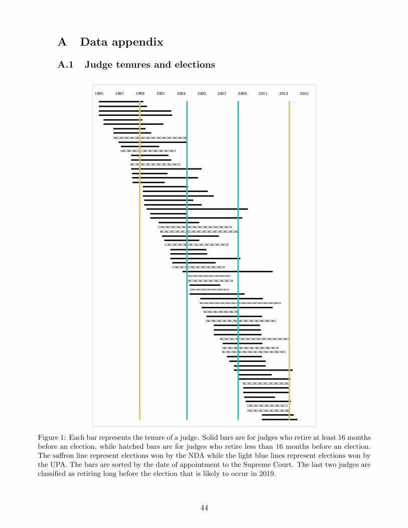
A Data appendix

A.1 Judge tenures and elections

1995 1997 1999 2001 2003 2005 2007 2009 2011 2013 2015

Figure 1: Each bar represents the tenure of a judge. Solid bars are for judges who retire at least 16 monthsbefore an election, while hatched bars are for judges who retire less than 16 months before an election.The saffron line represent elections won by the NDA while the light blue lines represent elections won bythe UPA. The bars are sorted by the date of appointment to the Supreme Court. The last two judges areclassified as retiring long before the election that is likely to occur in 2019.

44

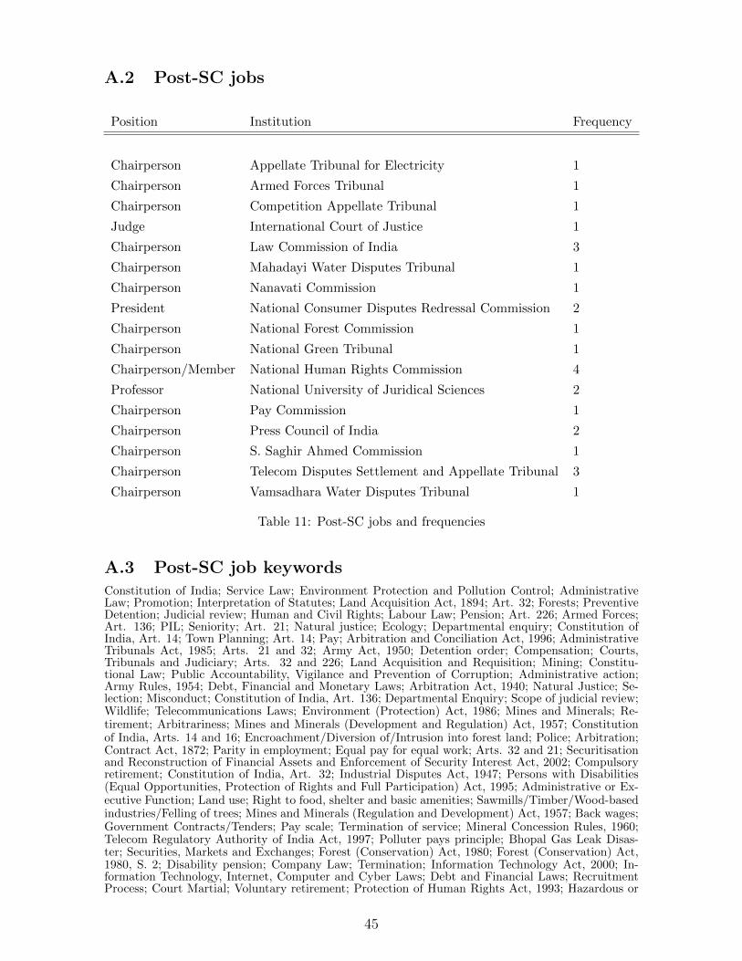
A.2 Post-SC jobs

Position Institution Frequency

Chairperson Appellate Tribunal for Electricity 1

Chairperson Armed Forces Tribunal 1

Chairperson Competition Appellate Tribunal 1

Judge International Court of Justice 1

Chairperson Law Commission of India 3

Chairperson Mahadayi Water Disputes Tribunal 1

Chairperson Nanavati Commission 1

President National Consumer Disputes Redressal Commission 2

Chairperson National Forest Commission 1

Chairperson National Green Tribunal 1

Chairperson/Member National Human Rights Commission 4

Professor National University of Juridical Sciences 2

Chairperson Pay Commission 1

Chairperson Press Council of India 2

Chairperson S. Saghir Ahmed Commission 1

Chairperson Telecom Disputes Settlement and Appellate Tribunal 3

Chairperson Vamsadhara Water Disputes Tribunal 1

Table 11: Post-SC jobs and frequencies

A.3 Post-SC job keywordsConstitution of India; Service Law; Environment Protection and Pollution Control; AdministrativeLaw; Promotion; Interpretation of Statutes; Land Acquisition Act, 1894; Art. 32; Forests; PreventiveDetention; Judicial review; Human and Civil Rights; Labour Law; Pension; Art. 226; Armed Forces;Art. 136; PIL; Seniority; Art. 21; Natural justice; Ecology; Departmental enquiry; Constitution ofIndia, Art. 14; Town Planning; Art. 14; Pay; Arbitration and Conciliation Act, 1996; AdministrativeTribunals Act, 1985; Arts. 21 and 32; Army Act, 1950; Detention order; Compensation; Courts,Tribunals and Judiciary; Arts. 32 and 226; Land Acquisition and Requisition; Mining; Constitu-tional Law; Public Accountability, Vigilance and Prevention of Corruption; Administrative action;Army Rules, 1954; Debt, Financial and Monetary Laws; Arbitration Act, 1940; Natural Justice; Se-lection; Misconduct; Constitution of India, Art. 136; Departmental Enquiry; Scope of judicial review;Wildlife; Telecommunications Laws; Environment (Protection) Act, 1986; Mines and Minerals; Re-tirement; Arbitrariness; Mines and Minerals (Development and Regulation) Act, 1957; Constitutionof India, Arts. 14 and 16; Encroachment/Diversion of/Intrusion into forest land; Police; Arbitration;Contract Act, 1872; Parity in employment; Equal pay for equal work; Arts. 32 and 21; Securitisationand Reconstruction of Financial Assets and Enforcement of Security Interest Act, 2002; Compulsoryretirement; Constitution of India, Art. 32; Industrial Disputes Act, 1947; Persons with Disabilities(Equal Opportunities, Protection of Rights and Full Participation) Act, 1995; Administrative or Ex-ecutive Function; Land use; Right to food, shelter and basic amenities; Sawmills/Timber/Wood-basedindustries/Felling of trees; Mines and Minerals (Regulation and Development) Act, 1957; Back wages;Government Contracts/Tenders; Pay scale; Termination of service; Mineral Concession Rules, 1960;Telecom Regulatory Authority of India Act, 1997; Polluter pays principle; Bhopal Gas Leak Disas-ter; Securities, Markets and Exchanges; Forest (Conservation) Act, 1980; Forest (Conservation) Act,1980, S. 2; Disability pension; Company Law; Termination; Information Technology Act, 2000; In-formation Technology, Internet, Computer and Cyber Laws; Debt and Financial Laws; RecruitmentProcess; Court Martial; Voluntary retirement; Protection of Human Rights Act, 1993; Hazardous or

45

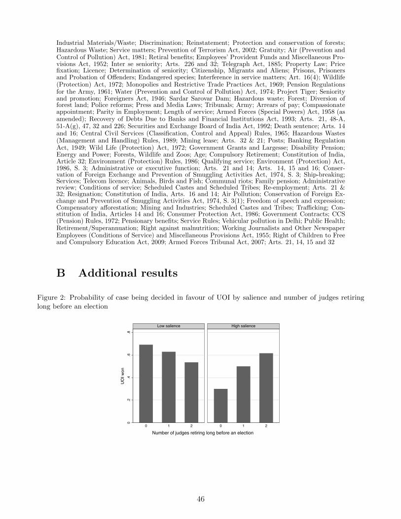
Industrial Materials/Waste; Discrimination; Reinstatement; Protection and conservation of forests;Hazardous Waste; Service matters; Prevention of Terrorism Act, 2002; Gratuity; Air (Prevention andControl of Pollution) Act, 1981; Retiral benefits; Employees’ Provident Funds and Miscellaneous Pro-visions Act, 1952; Inter se seniority; Arts. 226 and 32; Telegraph Act, 1885; Property Law; Pricefixation; Licence; Determination of seniority; Citizenship, Migrants and Aliens; Prisons, Prisonersand Probation of Offenders; Endangered species; Interference in service matters; Art. 16(4); Wildlife(Protection) Act, 1972; Monopolies and Restrictive Trade Practices Act, 1969; Pension Regulationsfor the Army, 1961; Water (Prevention and Control of Pollution) Act, 1974; Project Tiger; Seniorityand promotion; Foreigners Act, 1946; Sardar Sarovar Dam; Hazardous waste; Forest; Diversion offorest land; Police reforms; Press and Media Laws; Tribunals; Army; Arrears of pay; Compassionateappointment; Parity in Employment; Length of service; Armed Forces (Special Powers) Act, 1958 (asamended); Recovery of Debts Due to Banks and Financial Institutions Act, 1993; Arts. 21, 48-A,51-A(g), 47, 32 and 226; Securities and Exchange Board of India Act, 1992; Death sentence; Arts. 14and 16; Central Civil Services (Classification, Control and Appeal) Rules, 1965; Hazardous Wastes(Management and Handling) Rules, 1989; Mining lease; Arts. 32 & 21; Posts; Banking RegulationAct, 1949; Wild Life (Protection) Act, 1972; Government Grants and Largesse; Disability Pension;Energy and Power; Forests, Wildlife and Zoos; Age; Compulsory Retirement; Constitution of India,Article 32; Environment (Protection) Rules, 1986; Qualifying service; Environment (Protection) Act,1986, S. 3; Administrative or executive function; Arts. 21 and 14; Arts. 14, 15 and 16; Conser-vation of Foreign Exchange and Prevention of Smuggling Activities Act, 1974, S. 3; Ship-breaking;Services; Telecom licence; Animals, Birds and Fish; Communal riots; Family pension; Administrativereview; Conditions of service; Scheduled Castes and Scheduled Tribes; Re-employment; Arts. 21 &32; Resignation; Constitution of India, Arts. 16 and 14; Air Pollution; Conservation of Foreign Ex-change and Prevention of Smuggling Activities Act, 1974, S. 3(1); Freedom of speech and expression;Compensatory afforestation; Mining and Industries; Scheduled Castes and Tribes; Trafficking; Con-stitution of India, Articles 14 and 16; Consumer Protection Act, 1986; Government Contracts; CCS(Pension) Rules, 1972; Pensionary benefits; Service Rules; Vehicular pollution in Delhi; Public Health;Retirement/Superannuation; Right against malnutrition; Working Journalists and Other NewspaperEmployees (Conditions of Service) and Miscellaneous Provisions Act, 1955; Right of Children to Freeand Compulsory Education Act, 2009; Armed Forces Tribunal Act, 2007; Arts. 21, 14, 15 and 32

B Additional results

Figure 2: Probability of case being decided in favour of UOI by salience and number of judges retiringlong before an election

0.2

.4.6

.8

0 1 2 0 1 2

Low salience High salience

UOI w

on

Number of judges retiring long before an election

46

Table 12: Correlation between salience and bench retirement characteristics

(1) (2) (3) (4)

One retired long before 0.336∗∗∗ 0.232∗∗ 0.313∗∗∗ 0.211∗∗

(0.0991) (0.0989) (0.0949) (0.0832)

Both retired long before 0.317∗∗∗ 0.249∗∗ 0.288∗∗∗ 0.214∗∗∗

(0.117) (0.0995) (0.0904) (0.0791)

Case controls No Yes No Yes

Year dummies No No Yes Yes

Observations 662 662 662 662

R2 0.013 0.108 0.047 0.137

Dependent variable is the salience index. Case controls are type of case (appeal/petition), whethergovernment was appellant/petitioner, whether CJI was one of the judges, the tenures of the senior andjunior judge at the time of decision. Standard errors reported in the parentheses are clustered at thejudge dyad level. ∗ p < 0.1, ∗∗ p < 0.05, ∗∗∗ p < 0.01

47

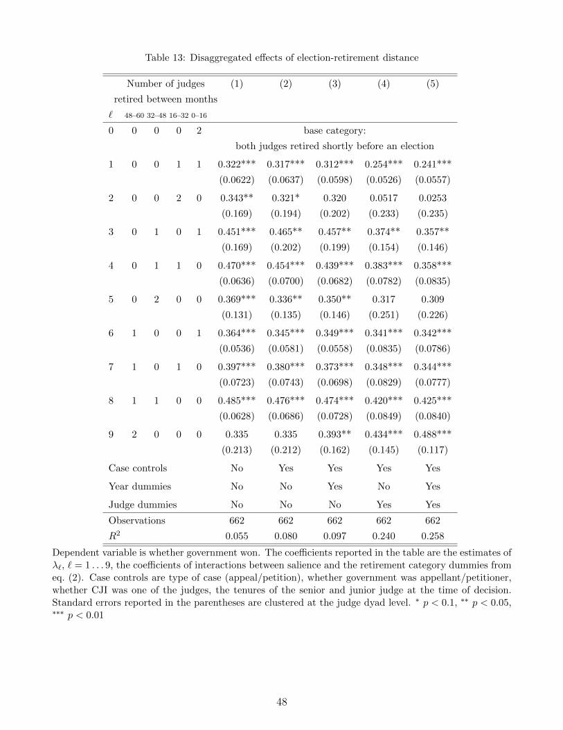
Table 13: Disaggregated effects of election-retirement distance

Number of judges (1) (2) (3) (4) (5)

retired between months

` 48–60 32–48 16–32 0–16

0 0 0 0 2 base category:

both judges retired shortly before an election

1 0 0 1 1 0.322*** 0.317*** 0.312*** 0.254*** 0.241***

(0.0622) (0.0637) (0.0598) (0.0526) (0.0557)

2 0 0 2 0 0.343** 0.321* 0.320 0.0517 0.0253

(0.169) (0.194) (0.202) (0.233) (0.235)

3 0 1 0 1 0.451*** 0.465** 0.457** 0.374** 0.357**

(0.169) (0.202) (0.199) (0.154) (0.146)

4 0 1 1 0 0.470*** 0.454*** 0.439*** 0.383*** 0.358***

(0.0636) (0.0700) (0.0682) (0.0782) (0.0835)

5 0 2 0 0 0.369*** 0.336** 0.350** 0.317 0.309

(0.131) (0.135) (0.146) (0.251) (0.226)

6 1 0 0 1 0.364*** 0.345*** 0.349*** 0.341*** 0.342***

(0.0536) (0.0581) (0.0558) (0.0835) (0.0786)

7 1 0 1 0 0.397*** 0.380*** 0.373*** 0.348*** 0.344***

(0.0723) (0.0743) (0.0698) (0.0829) (0.0777)

8 1 1 0 0 0.485*** 0.476*** 0.474*** 0.420*** 0.425***

(0.0628) (0.0686) (0.0728) (0.0849) (0.0840)

9 2 0 0 0 0.335 0.335 0.393** 0.434*** 0.488***

(0.213) (0.212) (0.162) (0.145) (0.117)




Observations 662 662 662 662 662

R2 0.055 0.080 0.097 0.240 0.258

Dependent variable is whether government won. The coefficients reported in the table are the estimates ofλ`, ` = 1 . . . 9, the coefficients of interactions between salience and the retirement category dummies fromeq. (2). Case controls are type of case (appeal/petition), whether government was appellant/petitioner,whether CJI was one of the judges, the tenures of the senior and junior judge at the time of decision.Standard errors reported in the parentheses are clustered at the judge dyad level. ∗ p < 0.1, ∗∗ p < 0.05,∗∗∗ p < 0.01

48

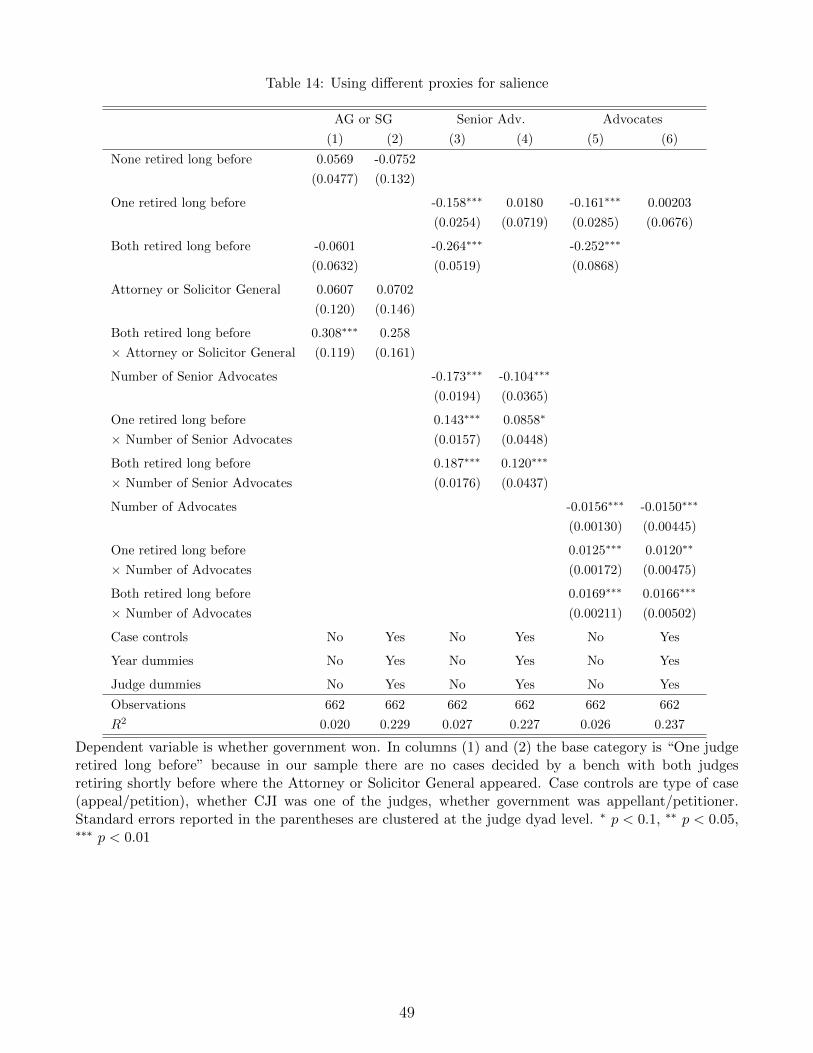
Table 14: Using different proxies for salience

AG or SG Senior Adv. Advocates

(1) (2) (3) (4) (5) (6)

None retired long before 0.0569 -0.0752

(0.0477) (0.132)

One retired long before -0.158∗∗∗ 0.0180 -0.161∗∗∗ 0.00203

(0.0254) (0.0719) (0.0285) (0.0676)

Both retired long before -0.0601 -0.264∗∗∗ -0.252∗∗∗

(0.0632) (0.0519) (0.0868)

Attorney or Solicitor General 0.0607 0.0702

(0.120) (0.146)

Both retired long before 0.308∗∗∗ 0.258

× Attorney or Solicitor General (0.119) (0.161)

Number of Senior Advocates -0.173∗∗∗ -0.104∗∗∗

(0.0194) (0.0365)

One retired long before 0.143∗∗∗ 0.0858∗

× Number of Senior Advocates (0.0157) (0.0448)

Both retired long before 0.187∗∗∗ 0.120∗∗∗

× Number of Senior Advocates (0.0176) (0.0437)

Number of Advocates -0.0156∗∗∗ -0.0150∗∗∗

(0.00130) (0.00445)

One retired long before 0.0125∗∗∗ 0.0120∗∗

× Number of Advocates (0.00172) (0.00475)

Both retired long before 0.0169∗∗∗ 0.0166∗∗∗

× Number of Advocates (0.00211) (0.00502)

Case controls No Yes No Yes No Yes

Year dummies No Yes No Yes No Yes

Judge dummies No Yes No Yes No Yes

Observations 662 662 662 662 662 662

R2 0.020 0.229 0.027 0.227 0.026 0.237

Dependent variable is whether government won. In columns (1) and (2) the base category is “One judgeretired long before” because in our sample there are no cases decided by a bench with both judgesretiring shortly before where the Attorney or Solicitor General appeared. Case controls are type of case(appeal/petition), whether CJI was one of the judges, whether government was appellant/petitioner.Standard errors reported in the parentheses are clustered at the judge dyad level. ∗ p < 0.1, ∗∗ p < 0.05,∗∗∗ p < 0.01

49

Table 15: Disaggregated effects by quartiles of salience

(1) (2) (3) (4) (5)

Salience (25–50 pctile) -0.179∗∗ -0.164∗∗∗ -0.148∗∗ -0.161∗∗ -0.134∗

(0.0753) (0.0621) (0.0632) (0.0796) (0.0799)

Salience (50–75 pctile) -0.290∗∗ -0.263∗∗ -0.241∗ -0.187 -0.159

(0.121) (0.127) (0.131) (0.121) (0.122)

Salience (75th) -0.529∗∗∗ -0.495∗∗∗ -0.504∗∗∗ -0.411∗∗ -0.413∗∗

(0.113) (0.113) (0.109) (0.171) (0.174)

One retired long before -0.120∗∗∗ -0.0996∗ -0.0953 -0.00696 0.00428

(0.0398) (0.0548) (0.0606) (0.0684) (0.0797)

Both retired long before -0.195∗∗∗ -0.161∗∗∗ -0.161∗

(0.0568) (0.0614) (0.0829)

One retired long before 0.00545 0.00645 -0.0132 0.0475 0.0125

× Salience (25–50 pctile) (0.102) (0.101) (0.0996) (0.0988) (0.103)

Both retired long before -0.00318 -0.0120 -0.0355 0.0201 -0.00921

× Salience (25–50 pctile) (0.0780) (0.0749) (0.0798) (0.0911) (0.101)

One retired long before 0.224∗∗ 0.237∗∗ 0.194 0.176 0.150

× Salience (50–75 pctile) (0.111) (0.116) (0.131) (0.125) (0.148)

Both retired long before 0.178 0.166 0.143 0.117 0.103

× Salience (50–75 pctile) (0.124) (0.133) (0.145) (0.143) (0.147)

One retired long before 0.320∗∗∗ 0.315∗∗∗ 0.307∗∗∗ 0.254 0.261

× Salience (75th) (0.112) (0.118) (0.118) (0.185) (0.177)

Both retired long before 0.510∗∗∗ 0.488∗∗∗ 0.492∗∗∗ 0.396∗∗ 0.402∗∗

× Salience (75th) (0.121) (0.122) (0.116) (0.197) (0.196)




Observations 662 662 662 662 662

R2 0.043 0.066 0.081 0.223 0.237

Dependent variable is whether government won. Case controls are type of case (appeal/petition), whetherCJI was one of the judges, whether government was appellant/petitioner. Standard errors reported inthe parentheses are clustered at the judge dyad level. ∗ p < 0.1, ∗∗ p < 0.05, ∗∗∗ p < 0.01

50

Table 16: Different thresholds for retired long before

(1) (2) (3) (4) (5) (6) (7) (8)

Threshold (months) 6 12 18 24 6 12 18 24

Salience -0.373∗∗∗ -0.365∗∗∗ -0.387∗∗∗ -0.137∗∗∗ -0.302∗∗∗ -0.266∗∗∗ -0.287∗∗∗ -0.115∗∗∗

(0.00606) (0.0728) (0.0501) (0.0232) (0.0576) (0.0598) (0.0417) (0.0420)

One retired long before -0.0123 0.0372 0.0548 -0.0234

(0.0591) (0.0437) (0.0403) (0.0489)

Both retired long before -0.116∗∗∗ 0.000520 0.0312 -0.109∗

(0.0376) (0.0647) (0.0760) (0.0661)

One retired long before 0.253∗∗∗ 0.298∗∗∗ 0.351∗∗∗ 0.114∗∗∗ 0.191∗∗∗ 0.218∗∗∗ 0.264∗∗∗ 0.104∗∗

× Salience (0.0186) (0.0791) (0.0656) (0.0306) (0.0695) (0.0734) (0.0557) (0.0468)

Both retired long before 0.389∗∗∗ 0.417∗∗∗ 0.434∗∗∗ 0.191∗∗∗ 0.318∗∗∗ 0.315∗∗∗ 0.330∗∗∗ 0.170∗∗∗

× Salience (0.0274) (0.0742) (0.0543) (0.0318) (0.0675) (0.0841) (0.0707) (0.0581)

Case controls No No No No Yes Yes Yes Yes

Year dummies No No No No Yes Yes Yes Yes

Judge dummies No No No No Yes Yes Yes Yes

Observations 662 662 662 662 662 662 662 662

R2 0.039 0.032 0.031 0.025 0.231 0.232 0.232 0.227

Dependent variable is whether government won. The column labels indicate the threshold in monthsat which a judge is considered to have retired long before an election. Case controls are type of case(appeal/petition), whether government was appellant/petitioner, whether CJI was one of the judges, thetenures of the senior and junior judge at the time of decision. Standard errors reported in the parenthesesare clustered at the judge dyad level. ∗ p < 0.1, ∗∗ p < 0.05, ∗∗∗ p < 0.01

51

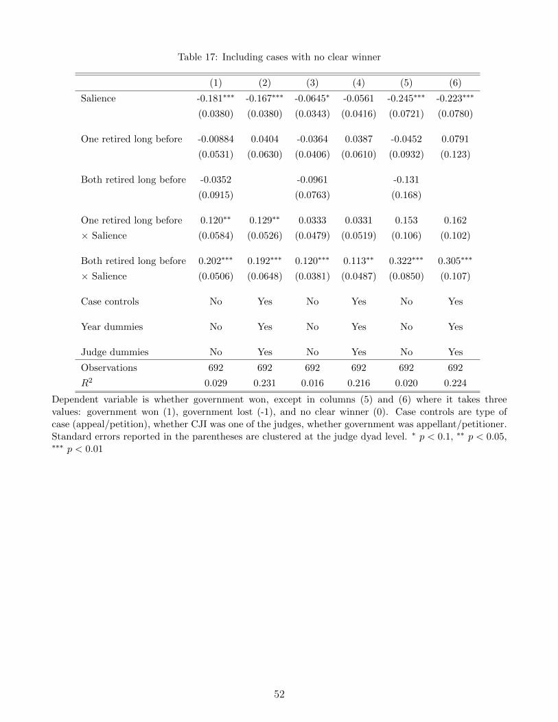
Table 17: Including cases with no clear winner

(1) (2) (3) (4) (5) (6)

Salience -0.181∗∗∗ -0.167∗∗∗ -0.0645∗ -0.0561 -0.245∗∗∗ -0.223∗∗∗

(0.0380) (0.0380) (0.0343) (0.0416) (0.0721) (0.0780)

One retired long before -0.00884 0.0404 -0.0364 0.0387 -0.0452 0.0791

(0.0531) (0.0630) (0.0406) (0.0610) (0.0932) (0.123)

Both retired long before -0.0352 -0.0961 -0.131

(0.0915) (0.0763) (0.168)

One retired long before 0.120∗∗ 0.129∗∗ 0.0333 0.0331 0.153 0.162

× Salience (0.0584) (0.0526) (0.0479) (0.0519) (0.106) (0.102)

Both retired long before 0.202∗∗∗ 0.192∗∗∗ 0.120∗∗∗ 0.113∗∗ 0.322∗∗∗ 0.305∗∗∗

× Salience (0.0506) (0.0648) (0.0381) (0.0487) (0.0850) (0.107)

Case controls No Yes No Yes No Yes

Year dummies No Yes No Yes No Yes

Judge dummies No Yes No Yes No Yes

Observations 692 692 692 692 692 692

R2 0.029 0.231 0.016 0.216 0.020 0.224

Dependent variable is whether government won, except in columns (5) and (6) where it takes threevalues: government won (1), government lost (-1), and no clear winner (0). Case controls are type ofcase (appeal/petition), whether CJI was one of the judges, whether government was appellant/petitioner.Standard errors reported in the parentheses are clustered at the judge dyad level. ∗ p < 0.1, ∗∗ p < 0.05,∗∗∗ p < 0.01

52

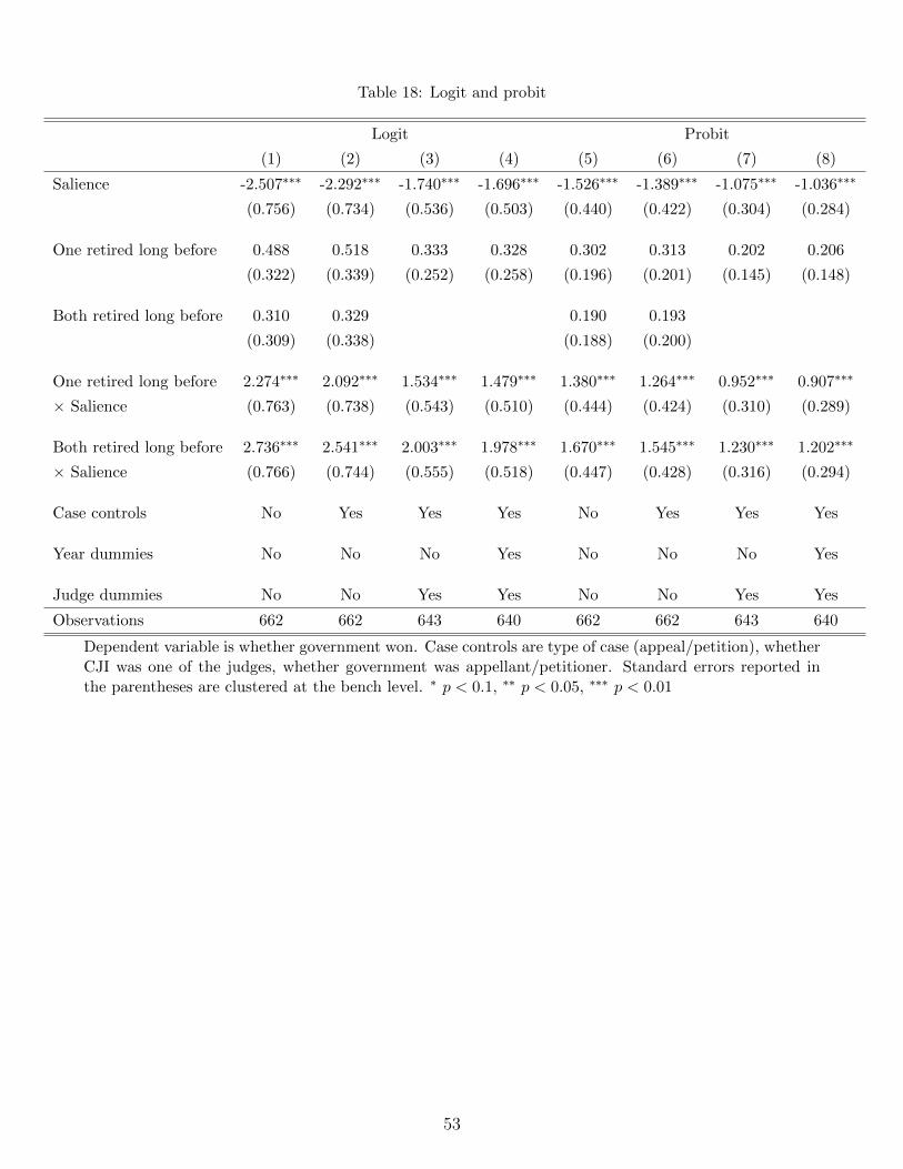
Table 18: Logit and probit

Logit Probit

(1) (2) (3) (4) (5) (6) (7) (8)

Salience -2.507∗∗∗ -2.292∗∗∗ -1.740∗∗∗ -1.696∗∗∗ -1.526∗∗∗ -1.389∗∗∗ -1.075∗∗∗ -1.036∗∗∗

(0.756) (0.734) (0.536) (0.503) (0.440) (0.422) (0.304) (0.284)

One retired long before 0.488 0.518 0.333 0.328 0.302 0.313 0.202 0.206

(0.322) (0.339) (0.252) (0.258) (0.196) (0.201) (0.145) (0.148)

Both retired long before 0.310 0.329 0.190 0.193

(0.309) (0.338) (0.188) (0.200)

One retired long before 2.274∗∗∗ 2.092∗∗∗ 1.534∗∗∗ 1.479∗∗∗ 1.380∗∗∗ 1.264∗∗∗ 0.952∗∗∗ 0.907∗∗∗

× Salience (0.763) (0.738) (0.543) (0.510) (0.444) (0.424) (0.310) (0.289)

Both retired long before 2.736∗∗∗ 2.541∗∗∗ 2.003∗∗∗ 1.978∗∗∗ 1.670∗∗∗ 1.545∗∗∗ 1.230∗∗∗ 1.202∗∗∗

× Salience (0.766) (0.744) (0.555) (0.518) (0.447) (0.428) (0.316) (0.294)

Case controls No Yes Yes Yes No Yes Yes Yes

Year dummies No No No Yes No No No Yes

Judge dummies No No Yes Yes No No Yes Yes

Observations 662 662 643 640 662 662 643 640

Dependent variable is whether government won. Case controls are type of case (appeal/petition), whetherCJI was one of the judges, whether government was appellant/petitioner. Standard errors reported inthe parentheses are clustered at the bench level. ∗ p < 0.1, ∗∗ p < 0.05, ∗∗∗ p < 0.01

53

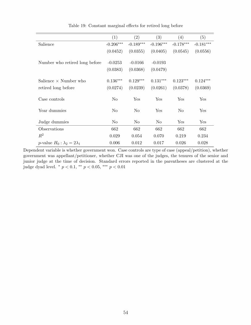
Table 19: Constant marginal effects for retired long before

(1) (2) (3) (4) (5)

Salience -0.206∗∗∗ -0.189∗∗∗ -0.196∗∗∗ -0.178∗∗∗ -0.181∗∗∗

(0.0452) (0.0355) (0.0405) (0.0545) (0.0556)

Number who retired long before -0.0253 -0.0166 -0.0193

(0.0383) (0.0368) (0.0479)

Salience × Number who 0.136∗∗∗ 0.129∗∗∗ 0.131∗∗∗ 0.123∗∗∗ 0.124∗∗∗

retired long before (0.0274) (0.0239) (0.0261) (0.0378) (0.0369)




Observations 662 662 662 662 662

R2 0.029 0.054 0.070 0.219 0.234

p-value H0 : λ2 = 2λ1 0.006 0.012 0.017 0.026 0.028


54

Table 20: At least one retired long before

(1) (2) (3) (4) (5)

Salience -0.387∗∗∗ -0.368∗∗∗ -0.374∗∗∗ -0.288∗∗∗ -0.285∗∗∗

(0.0502) (0.0613) (0.0668) (0.0423) (0.0447)

At least one retired long 0.0370 0.0590 0.0478

before (0.0507) (0.0596) (0.0818)

At least one retired long 0.379∗∗∗ 0.367∗∗∗ 0.369∗∗∗ 0.285∗∗∗ 0.282∗∗∗

before × Salience (0.0635) (0.0738) (0.0811) (0.0634) (0.0626)




Observations 662 662 662 662 662

R2 0.025 0.050 0.066 0.215 0.229


55

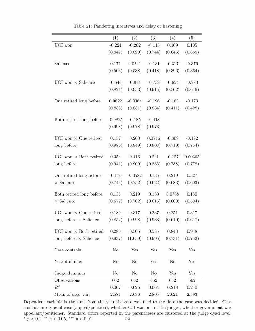
Table 21: Pandering incentives and delay or hastening

(1) (2) (3) (4) (5)

UOI won -0.224 -0.262 -0.115 0.169 0.105

(0.842) (0.829) (0.744) (0.645) (0.668)

Salience 0.171 0.0241 -0.131 -0.317 -0.376

(0.503) (0.538) (0.418) (0.396) (0.364)

UOI won × Salience -0.646 -0.814 -0.738 -0.654 -0.783

(0.821) (0.953) (0.915) (0.562) (0.616)

One retired long before 0.0622 -0.0364 -0.196 -0.163 -0.173

(0.833) (0.831) (0.834) (0.411) (0.428)

Both retired long before -0.0825 -0.185 -0.418

(0.998) (0.978) (0.973)

UOI won × One retired 0.157 0.260 0.0716 -0.309 -0.192

long before (0.980) (0.949) (0.903) (0.719) (0.754)

UOI won × Both retired 0.354 0.416 0.241 -0.127 0.00365

long before (0.941) (0.909) (0.835) (0.738) (0.778)

One retired long before -0.170 -0.0582 0.136 0.219 0.327

× Salience (0.743) (0.752) (0.622) (0.683) (0.603)

Both retired long before 0.136 0.219 0.150 0.0788 0.130

× Salience (0.677) (0.702) (0.615) (0.609) (0.594)

UOI won × One retired 0.189 0.317 0.237 0.251 0.317

long before × Salience (0.852) (0.998) (0.933) (0.610) (0.617)

UOI won × Both retired 0.280 0.505 0.585 0.843 0.948

long before × Salience (0.937) (1.059) (0.996) (0.731) (0.752)




Observations 662 662 662 662 662

R2 0.007 0.025 0.064 0.218 0.240

Mean of dep. var. 2.581 2.636 2.805 2.621 2.593

Dependent variable is the time from the year the case was filed to the date the case was decided. Casecontrols are type of case (appeal/petition), whether CJI was one of the judges, whether government wasappellant/petitioner. Standard errors reported in the parentheses are clustered at the judge dyad level.∗ p < 0.1, ∗∗ p < 0.05, ∗∗∗ p < 0.01 56

Table 22: Grandstanding and retirement-election distance

(1) (2) (3) (4)

Retired long before an -0.214 -0.175 -0.216 -0.204

election (0.153) (0.153) (0.147) (0.157)

Tenure 0.0644 -0.0212 -0.0154

(0.0416) (0.0506) (0.0529)

Constant 0.673∗∗∗ 0.317 0.690∗∗ 0.487

(0.132) (0.265) (0.287) (0.440)

Observations 72 72 72 72

R2 0.027 0.060 0.153 0.160

Dependent variable is the number of news articles in Factiva mentioning a judge during his SC tenuredivided by the length of tenure. Robust standard errors reported in the parentheses. ∗ p < 0.1, ∗∗

p < 0.05, ∗∗∗ p < 0.01

57

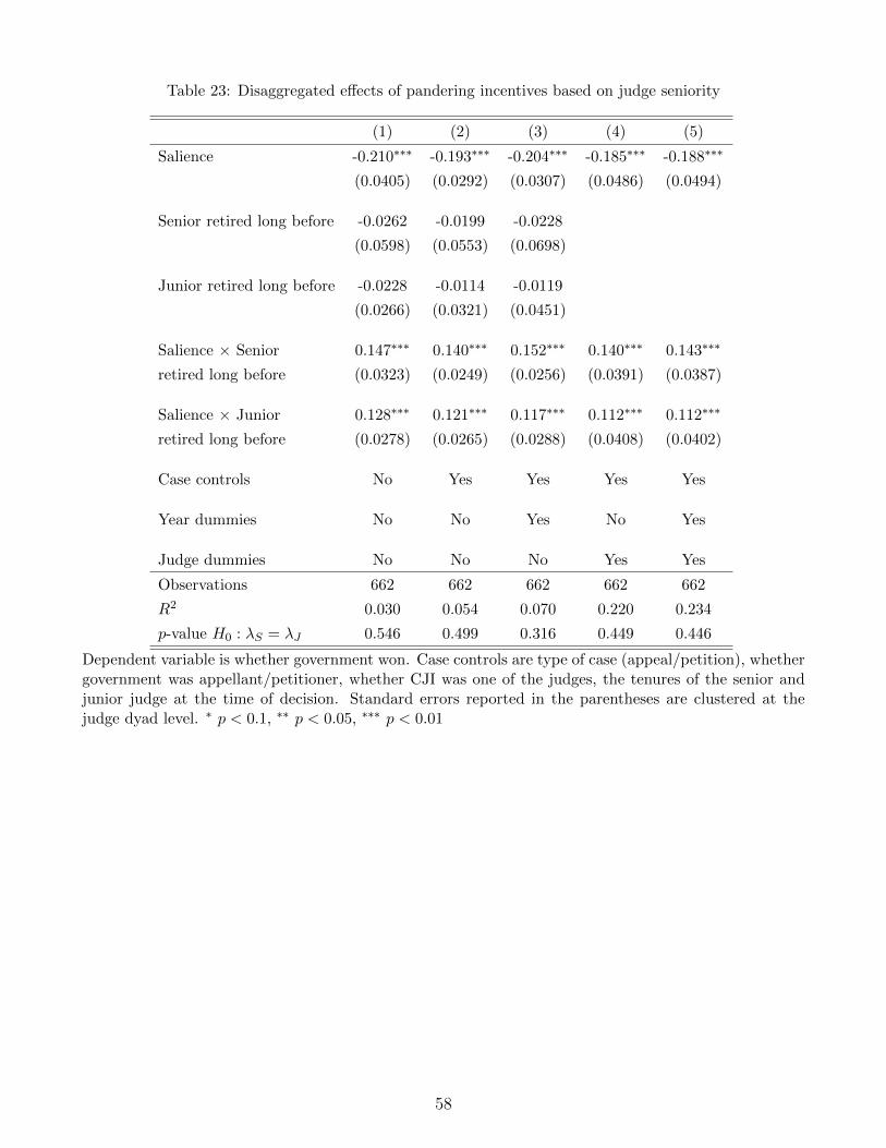
Table 23: Disaggregated effects of pandering incentives based on judge seniority

(1) (2) (3) (4) (5)

Salience -0.210∗∗∗ -0.193∗∗∗ -0.204∗∗∗ -0.185∗∗∗ -0.188∗∗∗

(0.0405) (0.0292) (0.0307) (0.0486) (0.0494)

Senior retired long before -0.0262 -0.0199 -0.0228

(0.0598) (0.0553) (0.0698)

Junior retired long before -0.0228 -0.0114 -0.0119

(0.0266) (0.0321) (0.0451)

Salience × Senior 0.147∗∗∗ 0.140∗∗∗ 0.152∗∗∗ 0.140∗∗∗ 0.143∗∗∗


Salience × Junior 0.128∗∗∗ 0.121∗∗∗ 0.117∗∗∗ 0.112∗∗∗ 0.112∗∗∗





Observations 662 662 662 662 662

R2 0.030 0.054 0.070 0.220 0.234

p-value H0 : λS = λJ 0.546 0.499 0.316 0.449 0.446


58

Table 24: Rewards for pandering (Logit)

75th pctile AG or SG(1) (2) (3) (4) (5) (6) (7) (8)

Number of cases, UOI won, 0.376∗∗ 0.392∗∗ 0.551∗∗ 0.545∗∗ 0.662∗∗ 0.661∗∗ 0.752∗∗ 0.816∗∗

salient, author (0.182) (0.177) (0.245) (0.248) (0.295) (0.292) (0.380) (0.384)




Tenure 0.267 0.313 0.233 0.227(0.351) (0.353) (0.340) (0.338)


Productivity 0.340 0.339 0.202 0.207(0.333) (0.333) (0.320) (0.307)

Constant -0.823 -1.538 -2.735 -2.974 -0.693 -1.394 -2.607 -2.548(1.302) (1.259) (2.302) (2.340) (1.234) (1.254) (2.243) (2.314)

Observations 70 70 70 70 70 70 70 70R2


59

Table 25: Rewards for pandering (Probit)

75th pctile AG or SG(1) (2) (3) (4) (5) (6) (7) (8)

Number of cases, UOI won, 0.232∗∗ 0.242∗∗ 0.342∗∗ 0.338∗∗ 0.416∗∗ 0.415∗∗ 0.475∗∗ 0.514∗∗

salient, author (0.103) (0.103) (0.141) (0.142) (0.179) (0.177) (0.229) (0.231)




Tenure 0.175 0.205 0.149 0.148(0.199) (0.202) (0.196) (0.194)


Productivity 0.215 0.215 0.127 0.130(0.202) (0.201) (0.194) (0.188)

Constant -0.502 -0.937 -1.742 -1.910 -0.431 -0.856 -1.633 -1.583(0.778) (0.775) (1.345) (1.369) (0.754) (0.770) (1.330) (1.381)

Observations 70 70 70 70 70 70 70 70R2


60

C Modelling endogenous litigant response

Let ex-post salience follow eq. (5), that is,

salienceik = ζ1I1k + ζ2I2k + ξ1 vi × I1k + ξ2 vi × I2k + vi. (12)

Let r ∈ {0, 1, 2} be the number of judges on the bench retiring long before. For brevity we

rename the variable both retired long beforek as Irk with r = 2 and one retired long beforek as

Irk with r = 1. Ex-ante salience vi is idiosyncratic across cases and unobserved. There is

no loss of generality38 in setting the coefficient on vi to 1. Since it is an indicator variable

Irk = I2rk. Moreover, the interaction of I1k and I2k, is always zero since each indicator is

active only when the other is inactive. Hence eq. (1) can be rewritten as

wonik = α0 +∑

jαjbjk +∑

tδtyit + β vi + (βζ1 + λ1ζ1) I1k + (βζ2 + λ2ζ2) I2k

+ (βξ1 + λ1ξ1 + λ1) vi × I1k + (βξ2 + λ2ξ2 + λ2) vi × I2k

+ (λ1ζ2 + λ2ζ1)I1k × I2k + (λ1ξ2 + λ2ξ1) vi × I1k × I2k + X′ikη + εik

= α0 +∑

jαjbjk +∑

tδtyit + β vi + (βζ1 + λ1ζ1) I1k + (βζ2 + λ2ζ2) I2k

+ (βξ1 + λ1ξ1 + λ1) vi × I1k + (βξ2 + λ2ξ2 + λ2) vi × I2k + X′ikη + εik

= α0 +∑

jαjbjk +∑

tδtyit + β vi + (βξ1 + λ1ξ1 + λ1) vi × I1k

+ (βξ2 + λ2ξ2 + λ2) vi × I2k + X′ikη + εik (13)

where the standalone effects of I1k and I2k are absorbed in the judge dummies, since retire-

ment characteristics are fixed for a judge over his tenure.

Using (13), we can recover the change in the probability of winning as we change the

ex-ante salience and the bench retirement characteristics:

∂wonik

∂vi|r=1 −

∂wonik

∂vi|r=0 = ξ1(β + λ1) + λ1

and similarly∂wonik

∂vi|r=2 −

∂wonik

∂vi|r=0 = ξ2(β + λ2) + λ2.

D Dyad-robust clustering

In this paper we have used dyad-robust clustering (Cameron and Miller 2014) to compute

standard errors. This form of clustering allows for correlation between error terms across

cases that have at least one judge in common.

This differs from two-way clustering since two-way clustering imposes a particular struc-

ture on the correlations that is unsuitable for our context. Applying standard two-way cluster-

38Were vi to appear with a positive multiplicative constant φ, we could simply rescale and define viφ as ex-ante

salience so that salienceik = ζ1I1k + ζ2I2k + ξ1 vi × I1k + ξ2 vi × I2k + vi where ξ = ξφ .

61

ing to our regressions would require the use of two clustering variables reflecting the identity

of the judges deciding a case. Any choice of such variables, such as first and second judge

by alphabetical order of name, senior and junior judge, author and non-author, imposes the

following arbitrary restriction: error terms across two cases are treated as being uncorrelated

if the judge appearing in both cases is the first judge in a case and the second judge in the

other. Dyad-robust clustering generalises two-way clustering by allowing correlations in the

error terms across any two cases that share a common judge.

Note that dyad-robust clustering also subsumes clustering at the bench level. Clustering

at the bench level assumes that the error terms in cases decided by different benches are

uncorrelated. However, this assumption is too strong in our context since there may be

correlation across the error terms for the cases decided by the same judge when he appears

in different benches. Dyad-robust clustering allows for such correlation. Nonetheless, our

results are robust to clustering at the bench level. These are available upon request.

62

jobs for justice(s): corruption in the supreme court of … · corruption in the supreme court of...

Documents