joachim grammig, erik theissen, and oliver wünsche · joachim grammig, erik theissen, and oliver...
TRANSCRIPT
Center for Financial Studies Goethe-Universität Frankfurt House of Finance
Grüneburgplatz 1 60323 Frankfurt Deutschland
Telefon: +49 (0)69 798-30050 Fax: +49 (0)69 798-30077 http://www.ifk-cfs.de E-Mail: [email protected]
No. 2011/08
Time and the Price Impact of a Trade: A Structural Approach
Joachim Grammig, Erik Theissen, and Oliver Wünsche

Center for Financial Studies Goethe-Universität House of Finance
Grüneburgplatz 1 60323 Frankfurt am Main Deutschland
Telefon: +49 (0)69 798-30050 Fax: +49 (0)69 798-30077 http://www.ifk-cfs.de E-Mail: [email protected]
Center for Financial Studies
The Center for Financial Studies is a nonprofit research organization, supported by an association of more than 120 banks, insurance companies, industrial corporations and public institutions. Established in 1968 and closely affiliated with the University of Frankfurt, it provides a strong link between the financial community and academia.
The CFS Working Paper Series presents the result of scientific research on selected topics in the field of money, banking and finance. The authors were either participants in the Center´s Research Fellow Program or members of one of the Center´s Research Projects.
If you would like to know more about the Center for Financial Studies, please let us know of your interest.
Prof. Michalis Haliassos, Ph.D. Prof. Dr. Jan Pieter Krahnen Prof. Dr. Uwe Walz
* Earlier versions of the paper were presented at the ESF workshop on High Frequency Econometrics at Warwick University, the Conference on the Microstructure of Financial Markets in Europe at the University of Constance, and meetings of the European Finance Association (Ljublijana, Slovenia), and the German Finance Association (Dresden). We are especially grateful to Ekkehart Boehmer, Miroslav Budimir, Alfonso Dufour, Stefan Frey, Daniel Mayston, Winfried Pohlmeier and Uwe Schweickert for offering helpful comments. We thank the German Stock Exchange for data sponsorship, and the German Research Foundation (DFG) as well as the CFR for financial support. We assume responsibility for any remaining errors.
1 University of Tübingen, Centre for Financial Research (CFR), Cologne, and Center for Financial Studies, Frankfurt. Contact Details:
University of Tübingen, Department of Business Administration and Economics, Mohlstr. 36, 72074 Tübingen, Germany; Phone: +49 7071 2976009, Fax: +49 7071 295546; E-mail: [email protected]
2 University of Mannheim, Centre for Financial Research (CFR), Cologne, and Center for Financial Studies, Frankfurt. Contact Details:
University of Mannheim, Finance Area, L 5, 2, 68131Mannheim, Germany; Phone: +49 621 181 1517, Fax: +49 621 181 1519; E-mail: [email protected]
3 UBS AG, Group Risk Methodology, Stockerstrasse 64, P.O. Box 8002 Zurich, Switzerland; Phone: +41 44 234 7106; E-mail:
CFS Working Paper No. 2011/08
Time and the Price Impact of a Trade:
A Structural Approach *
Joachim Grammig1, Erik Theissen2, and Oliver Wünsche3,
Febuary 9, 2011
Abstract: We revisit the role of time in measuring the price impact of trades using a new empirical method that combines spread decomposition and dynamic duration modeling. Previous studies which have addressed the issue in a vector-autoregressive framework conclude that times when markets are most active are times when there is an increased presence of informed trading. Our empirical analysis based on recent European and U.S. data offers challenging new evidence. We find that as trade intensity increases, the informativeness of trades tends to decrease. This result is consistent with the predictions of Admati and Pfleiderer’s (1988) rational expectations model, and also with models of dynamic trading like those proposed by Parlour (1998) and Foucault (1999). Our results cast doubt on the common wisdom that fast markets bear particularly high adverse selection risks for uninformed market participants. JEL Classification: G10, C32 Keywords: Price Impact of Trades, Trading Intensity, Dynamic Duration Models, Spread
Decomposition Models, Adverse Selection Risk
1 Introduction
How is the time interval between transactions associated with information processing in
financial markets? If a high trading intensity indicates the presence of informed traders,
should a liquidity trader steer clear of an active market in order to avoid adverse selection?
And is it prudent to protect non-informed agents by interrupting continuous trading in
a fast market (and re-start with a call auction)? These are important questions for aca-
demics, traders and exchange operators alike, and they have spurred a growing theoretical
and empirical body of literature.1 In a seminal paper, Dufour and Engle (2000) extend
Hasbrouck’s (1991a, 1991b) vector-autoregressive framework to account for time-varying
transaction intensity when measuring the informational content of trades. Dufour and
Engle’s (2000) findings are in line with a conventional wisdom of market microstructure:
that fast trading means informed trading.
This paper revisits the role of time in measuring the price impact of trades. We combine
Madhavan et al.’s (1997) spread decomposition model and the autoregressive conditional
duration (ACD) model introduced by Engle and Russell (1998), and study how time-
varying trade intensities affect the adverse selection component of the spread. Our empir-
ical findings, based on recent European and US data, contradict the “fast trading means
informed trading” paradigm. They indicate that short time intervals between trades rather
reflect the activity of impatient, yet uninformed traders. Our results thus re-emphasize
the empirical relevance of Admati and Pfleiderer’s (1988) rational expectations model and
strategic trading models like those of Parlour (1998) and Foucault (1999). Our study casts
doubt on the common wisdom that fast markets bear particularly high adverse selection
risks for uninformed market participants.
Classic microstructure theory delivers ambiguous predictions regarding the relation be-
tween transaction intensities and informativeness of trade events. Diamond and Verrecchia
(1987) show that in the presence of short sale constraints, longer intervals of trade inac-
tivity indicate bad news. In Easley and O’Hara’s (1992) model, informed traders split up
1See Hasbrouck (2007) and Biais et al. (2005) for recent surveys.
2
their orders into smaller chunks in order to conceal their information. This behavior leads
to shorter durations between trades. In the same vein, Foster and Viswanathan (1990)
explain high activity by the presence of informed traders, which deters the uninformed
from trading. A contradictory prediction follows from Admati and Pfleiderer’s (1988)
model. Here, non-informed liquidity traders cluster during certain periods of the trading
day, which implies that trades in a fast market are less informative. Dufour and Engle’s
(2000) finding that trades occurring after short time intervals since the last transaction
are associated with a larger price impact than trades following long non-trading periods
thus corroborates the “fast trading means informed trading” hypothesis implied by Easley
and O’Hara’s (1992) model. This conclusion is supported by Furfine (2007) and Spierdijk
(2004), who also use VAR approaches based on midquote returns.
We contribute to the discussion from a different methodological angle. Instead of
using a multiple time series model, we draw on the class of spread decomposition models
put forth by Glosten and Harris (1988), Madhavan et al. (1997) and Huang and Stoll
(1997). The key parameter in Madhavan et al.’s (1997) model is the adverse selection
component of the spread, which indicates how liquidity suppliers assess the price impact of
incoming trades. We model the adverse selection component as a time-varying parameter
which depends on the time between trades. These trade durations are highly predictable,
exhibiting a pronounced diurnal pattern and a strong serial correlation (c.f. Engle and
Russell 1998). Since only the unpredictable component should have new informational
content, we identify the innovation component of the trade duration process using the
ACD model developed by Engle and Russell (1998). We derive moment conditions that
allow the joint estimation of structural and autoregressive parameters using the Generalized
Method of Moments (GMM). Our methodological contribution is thus to establish a link
between classic microstructure and the econometrics of ultra-high frequency data initiated
by Engle (2000).
Our empirical analysis is based on a cross-section of stocks traded on one of the most
important European stock markets, the Frankfurt Stock Exchange’s Xetra system, as well
as a matched sample of NYSE-traded U.S. stocks. Our results contradict the “fast trading
3
means informed trading” paradigm. For both the European and the US samples we find
that transactions occurring during periods of high trading activity are less informative than
trades during less active periods. Moreover, the adverse selection component of the spread
is considerably smaller for trades after shorter durations. This finding is in sharp contrast
to the results of Dufour and Engle (2000). It is, however, in accordance with Admati and
Pfleiderer’s (1988) rational expectations model, and it is also consistent with the crowding-
out effect described in Parlour (1998), which works - in a nutshell - as follows. When spreads
are small and depth at the best quotes is high, the probability of execution of a limit order
decreases and, consequently, limit orders become less advantageous. Impatient traders will
thus switch to using market orders. The crowding-out of limit orders by market orders
results in an increased trading frequency and shorter inter-trade durations. But periods
of ample liquidity are associated with low price volatility and no asymmetric information.
Thus, active markets are expected to imply small price impacts of trades.
When we estimate Dufour and Engle’s (2000) VAR on our data, we are able to qual-
itatively confirm their findings and the resulting conclusions. The contradictory results
must therefore be rooted in the way the empirical methodologies make use of the data. We
argue that by thinning the sequence of quote changes at trade events, a self-selected sam-
ple is produced. The trade-event filtering performed by Dufour and Engle (2000) implies
that all quote revisions in between trades are implicitly associated with the previous trade
event. However, midquote changes can occur due to the processing of public information
unrelated to the previous trade event. We argue, therefore, that the trade-event filtering
of quote revisions drives the “fast trading means informed trading” result. The key differ-
ence between Dufour/Engle’s VAR and our structural alternative is that we do not rely on
filtered observed quote revisions, but assume that the suppliers of liquidity anticipate the
information revealed in subsequent trades. 2
2The obvious solution (at first sight) estimating the trade and quote VAR on non-filtered data is not feasible.When pure quote revision events are included in the data, the VAR parameters cannot be made dependenton the time between trades.
4
The remainder of the paper is organized as follows. In Section 2 we describe the market
structure and the data, before going on to explain our empirical methodology in Section
3. The empirical results are then presented and discussed in Sections 4 and 5, before we
conclude our analysis in Section 6.
2 Market structure and data
Our empirical analysis uses data from the first quarter of 2004 from one of the largest
European Stock markets, the open limit order book system Xetra operating at the Frank-
furt Stock Exchange (FSE) together with a matched sample of NYSE stocks. The trading
process at the NYSE is well known, so we will focus on a brief description of the FSE-Xetra
trading environment. In Europe, FSE-Xetra is runner up in terms of turnover after the
London Stock Exchange.3 The trading rules are similar to other limit order book markets
around the world like Euronext, the Hong Kong Stock Exchange and the Australian Stock
Exchange. Between an opening and a closing call auction - and interrupted by another
mid day call auction - FSE-Xetra operates as a continuous double auction mechanism with
automatic matching of orders based on price and time priority. The transparency of the
market is only limited by the existence of hidden orders. These are (typically large) limit
orders with the special provision that a portion of the volume is initially kept hidden and
is thus not visible in the otherwise open book.
During the sample period, trading hours extended from 9.00 a.m. to 5.30 p.m.Central
European Time. No dedicated market makers are employed for the DAX stocks.4 FSE-
Xetra competes for order flow with some regional and international exchanges. The FSE
itself maintains a parallel floor trading system and some of our sample stocks were also
3According to data from September 2008 to September 2009 published by the World Federation of Exchanges(http://www.world-exchanges.org/statistics/ytd-monthly). The Xetra system also operates at the Irishand the Vienna Stock Exchange, the European Energy Exchange and the Shanghai Stock Exchange,China’s largest securities market.
4For less actively traded stocks there are so-called Designated Sponsors - typically large banks - who arerequired to provide a minimum liquidity level by simultaneously submitting competitive buy and sell limitorders.
5
cross-listed at the NYSE. However, for those stocks considered in our study, FSE-Xetra
clearly dominates the regional and international competitors in terms of market share.
Our data contain detailed information about all market events which occurred during
the first quarter of 2004. Based on these event histories, we perform a real-time recon-
struction of the sequences of best bid and ask prices and associated depth, time stamps,
transaction prices and trade volumes. One of the major advantages is that it is possible to
unambiguously identify whether a trade is buyer- or seller-initiated (something that is not
possible using the NYSE TAQ data). This avoids the biases that haunt the estimation of
structural parameters when the trade classification is error-prone (c.f. Boehmer et al. 2007).
insert Table 1 about here
Table 1 reports market capitalization, daily turnover, average daily number of trades,
average price, and the average quoted spread for our German sample, which consists of the
thirty stocks constituting the DAX30 index. The daily turnover of an average stock is about
109 million Euros, with 2100 daily trades per stock. The mean relative effective spread
amounts to 0.08 percent (3 Euro cent) and the mean relative realized spread is 0.01 percent
(0.2 Euro cent), indicating a liquid market.5 The table also displays how the securities are
sorted into four groups according to their trading frequency (activity quartiles). Group
one contains the most actively traded stocks, while group four is comprised of the least
frequently traded stocks. We also construct a matched sample of NYSE-listed stocks
using the daily trading volume as matching criterion, with the data taken from the TAQ
files supplied by the NYSE. Information about the NYSE sample is provided in Table
2. Throughout the paper we focus on the German sample and treat the US sample as a
robustness check, as the German data allows trades to accurately be classified as either
buyer- or seller-initiated.
insert Table 2 about here
5We define the realized spread as the difference between the transaction price and the quote midpoint after10 minutes, multiplied by a trade indicator variable (1 for buyer-initiated trades, -1 for seller-initiatedtrades).
6
3 Methodology
3.1 Dufour and Engle’s trade and quote VAR
Before we describe our alternative methodology it is helpful to review how Dufour and
Engle (2000) quantify the role of time when measuring the price impact of a trade. Drawing
on Hasbrouck’s (1991a, 1991b) seminal work, they specify the following bivariate vector-
autoregression (VAR),
Ri =5
∑
j=1
ajRi−j + γopenDiQi +5
∑
j=0
bj,iQi−j + v1,i (1)
Qi =
5∑
j=1
cjRi−j + γopenDi−1Qi−1 +
5∑
j=1
djQi−j + v2,i, (2)
where bj,i = γj + δj ln(Ti−j). The trade indicator Qi takes the value of one if the ith trade
is buyer-initiated and minus one if it is seller-initiated. Ri denotes the midquote change in
response to the ith trade. Di indicates the first trade of the day. Ti measures the length
of the time interval between the ith trade occurring at calender time ti and the previous
trade at time ti−1 (trade duration). The larger bj,i (> 0), the greater the price impact of a
trade. Whether a shorter trade duration implies that a trade has increasing or decreasing
informativeness depends on the parameters δj . Negative δj imply that transactions occur-
ring after short trade durations are more informative than those after a longer non-trading
interval. As the computation of Hasbrouck’s (1991a) trade informativeness measure is not
possible, Dufour and Engle (2000) use illustrative impulse response functions to quantify
the overall effect of time between trades on trade informativeness6
6Hasbrouck (1991a) uses the MA(∞) representation of his bivariate trade and quote VAR to compute thepermanent impact of a trade on the midquote. The time-varying parameters bi,j in (1) render Hasbrouck’strade-informativeness measure time-varying as well. We will return to this issue in Section 5.
7
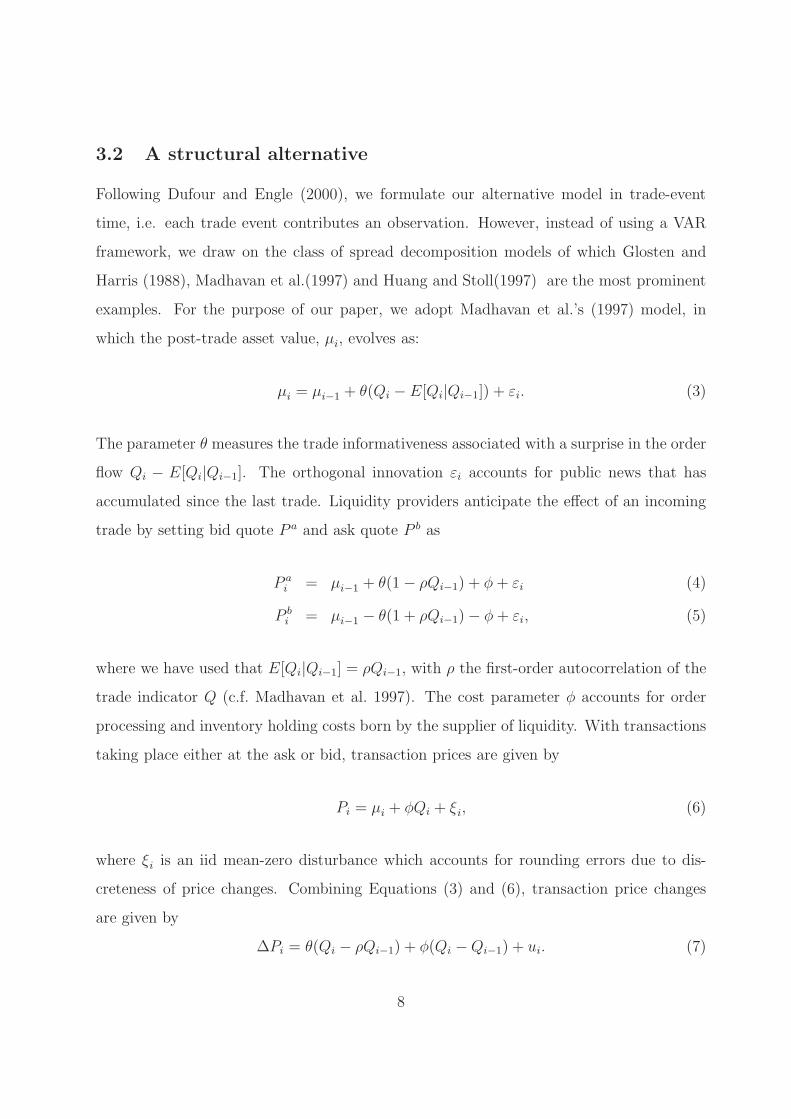
3.2 A structural alternative
Following Dufour and Engle (2000), we formulate our alternative model in trade-event
time, i.e. each trade event contributes an observation. However, instead of using a VAR
framework, we draw on the class of spread decomposition models of which Glosten and
Harris (1988), Madhavan et al.(1997) and Huang and Stoll(1997) are the most prominent
examples. For the purpose of our paper, we adopt Madhavan et al.’s (1997) model, in
which the post-trade asset value, µi, evolves as:
µi = µi−1 + θ(Qi − E[Qi|Qi−1]) + εi. (3)
The parameter θ measures the trade informativeness associated with a surprise in the order
flow Qi − E[Qi|Qi−1]. The orthogonal innovation εi accounts for public news that has
accumulated since the last trade. Liquidity providers anticipate the effect of an incoming
trade by setting bid quote P a and ask quote P b as
P ai = µi−1 + θ(1− ρQi−1) + φ+ εi (4)
P bi = µi−1 − θ(1 + ρQi−1)− φ+ εi, (5)
where we have used that E[Qi|Qi−1] = ρQi−1, with ρ the first-order autocorrelation of the
trade indicator Q (c.f. Madhavan et al. 1997). The cost parameter φ accounts for order
processing and inventory holding costs born by the supplier of liquidity. With transactions
taking place either at the ask or bid, transaction prices are given by
Pi = µi + φQi + ξi, (6)
where ξi is an iid mean-zero disturbance which accounts for rounding errors due to dis-
creteness of price changes. Combining Equations (3) and (6), transaction price changes
are given by
∆Pi = θ(Qi − ρQi−1) + φ(Qi −Qi−1) + ui. (7)
8

where ui = εi + ξi − ξi−1.
We account for the role of time in measuring the price impact of trade by specifying
the adverse selection parameter θ as a function of the duration since the last trade. Our
first specification is similar to that of Dufour and Engle’s VAR in that raw trade durations
(Ti) determine the price impact of trades,
φ(ti) = γφ +
M∑
m=1
λφmdm,i (8)
θ(Ti, ti) = γθ +M∑
m=1
λθmdm,i + δ lnTi, (9)
where dm,i equals one if the ith trade occurs within themth ofM time-of-day bins and is zero
otherwise. γφ, γθ, λφm and λθm are parameters. Allowing the adverse selection parameter θ
and the cost parameter φ to be time-of-day dependent accounts for the ∪−shaped time-of-
day pattern of the spread. Our specification bears resemblance to that of Dufour and Engle
(2000) in that sign and size of the parameter δ indicate whether a high trading activity is
associated with increased (δ < 0) or reduced trade informativeness (δ > 0).
insert Figure 1 about here
However, it is only the unexpected component of the trade duration process that should
carry informational content with respect to the fundamental asset value µ, as changes in µ
should be unpredictable. Yet it is well known that trade durations are highly predictable
(c.f. Engle and Russell 1998). They exhibit a clear-cut, inverted ∪-shaped intra-day (di-
urnal) pattern (see Figure 1), and significant serial correlation even after correcting for
diurnality. In our second specification we therefore assume that rather than raw trade du-
rations, duration shocks, innovations to the duration process, determine the price impact
of a trade:
θ(νi, ti) = γθ +M∑
m=1
λθmdm,i + δ ln νi. (10)
νi denotes the unexpected component of the trade duration process. To identify these
duration shocks, we follow Engle and Russell (1998) and separate the trade duration process
9

into a deterministic time-of-day component, Φ(ti), an autoregressive component, ψi, and
an innovation component, νi,
Ti = Φ(ti)ψiνi, (11)
where E(νi) = 1. The autoregressive component ψi evolves as
ψi = ω + αTi−1 + βψi−1, (12)
where Ti = Ti/Φ(ti). Equations 11 and 12 constitute Engle and Russell’s (1998) ACD
model. The conditional expected duration is given by Φ(ti)ψi, and νi is the innovation in
the duration process we seek to identify. We will refer to a model where transaction price
change are given by
∆Pi =(
γφ +M∑
m=1
λφmdm,i
)
Qi −(
γφ +M∑
m=1
λφmdm,i−1
)
Qi−1
+(
γθ +
M∑
m=1
λθmdm,i + δ ln νi
)
(Qi − ρQi−1) + ui (13)
as the MRR-ACD model.
3.3 Estimation
We propose a two-step procedure to estimate the MRR-ACD parameters. Following Engle
and Russell (1998), we first estimate the time-of-day function Φ(ti) using a polynomial
trigonometric regression (Eubank and Speckman 1990) and compute diurnally-adjusted
durations as Ti = Ti/Φ(ti). In a second step, GMM estimates of the MRR-ACD parameter
vector θ = (γφ, λφ1 , . . . , λφM , γ
θ, λθ1, . . . , λθM , ρ, ω, α, β, δ)
′ are computed based on the moment
10
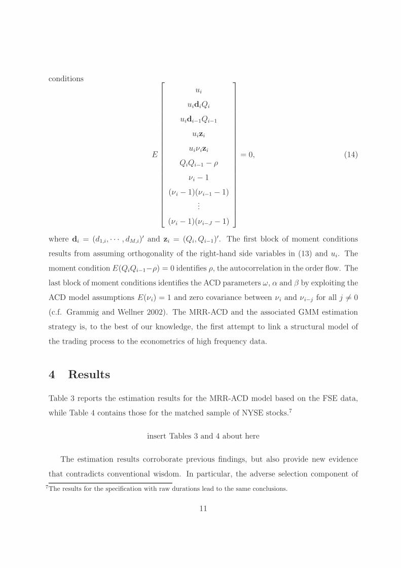
conditions
E
ui
uidiQi
uidi−1Qi−1
uizi
uiνizi
QiQi−1 − ρ
νi − 1
(νi − 1)(νi−1 − 1)...
(νi − 1)(νi−J − 1)
= 0, (14)
where di = (d1,i, · · · , dM,i)′ and zi = (Qi, Qi−1)
′. The first block of moment conditions
results from assuming orthogonality of the right-hand side variables in (13) and ui. The
moment condition E(QiQi−1−ρ) = 0 identifies ρ, the autocorrelation in the order flow. The
last block of moment conditions identifies the ACD parameters ω, α and β by exploiting the
ACD model assumptions E(νi) = 1 and zero covariance between νi and νi−j for all j 6= 0
(c.f. Grammig and Wellner 2002). The MRR-ACD and the associated GMM estimation
strategy is, to the best of our knowledge, the first attempt to link a structural model of
the trading process to the econometrics of high frequency data.
4 Results
Table 3 reports the estimation results for the MRR-ACD model based on the FSE data,
while Table 4 contains those for the matched sample of NYSE stocks.7
insert Tables 3 and 4 about here
The estimation results corroborate previous findings, but also provide new evidence
that contradicts conventional wisdom. In particular, the adverse selection component of
7The results for the specification with raw durations lead to the same conclusions.
11
the spread λθ is considerably higher during the first half hour of the trading day. The L-
shaped time-of-day pattern of the adverse selection component is most pronounced for less
frequently traded stocks (see Figure 2), while the part of the adverse selection component
that can be attributed to duration shocks does not exhibit a discernible diurnal pattern.
The estimates of the λφ parameters imply that the order processing cost component is
significantly higher at the end of the day, consistent with the notion that liquidity providers
demand compensation for holding overnight inventory. These findings are in accordance
with Madhavan et al.’s (1997) explanation of the ∪-shaped diurnal pattern of the effective
spread.
insert Figure 2 about here
In order to assess the plausibility of the estimation results, in Table 5 we report the
cross-sectional correlations of MRR-ACD-implied spread components with observable stock
characteristics as well as with model-free estimates of spread components. The correlation
between the model-implied spread and the effective spread amounts to 0.996, and the
correlation between the implied adverse selection component and the price impact is 0.965.
The correlation between the implied non-information-related component of the spread and
the realized spread is 0.881. The negative correlations between the implied adverse selection
component and market capitalization and trading activity, respectively, conform the well-
known result that adverse selection effects are exacerbated for small-cap and less frequently
traded stocks. All in all, these results illustrate the economic plausibility of the MRR-ACD
specification.
insert Table 5 about here
The results discussed so far are both conclusive and unobtrusive. However, the esti-
mated relation between a trade duration shock and trade informativeness contradicts the
“fast trading means informed trading” paradigm. For the FSE sample, the estimates of the
key parameter δ in MRR-ACD Equation (10) are positive and significantly different from
zero for all stocks. In the NYSE sample, the estimate of δ is positive and significant for 25
12
of the 30 stocks. None of the estimates is negative (c.f. Tables 3 and 4). This implies that
a shorter time interval since the last trade tends to be associated with reduced informa-
tional content pertaining to the next trade. This result, and the conclusions that can be
derived from it, are in sharp contrast to the findings that Dufour and Engle (2000) report.
In their VAR analysis, the estimates of the δj parameters (Equation (1)) are significantly
negative, which suggests that shorter trade durations imply that incoming trades have a
greater price impact.
Before we provide and discuss explanations for these contradictory findings, let us assess
the economic significance of our estimation results. Although we focus on the FSE sample,
the story for the NYSE sample is qualitatively similar.
insert Figures 3 and 4 about here
Figures 3 and 4 illustrate the importance of time in measuring the price impact of trades.
To provide a concise view, we sort all trade events for a specific stock or activity quartile
by the size of the duration shock. We then group the trade observations into deciles, with
the first decile encompassing the trades associated with the smallest duration shocks, and
decile ten the trades with the largest duration shocks. For each decile, the standardized
adverse selection component is averaged across trades.8 Figure 3 shows that for the quartile
of least actively traded stocks, the standardized adverse selection component more than
triples from duration decile one to duration decile ten. Figure 4 depicts the decile plots
for four representative stocks, one from each of the trade activity quartiles. The negative
relation between trade duration shocks and trade informativeness is very similar across the
four stocks.9
8Standardization is performed by dividing the adverse selection component θ(νi, ti) by the average midquoteacross the sample (P ). Using non-standardized adverse selection components yields similar results. Weuse the standardized components to enhance comparability across stocks. The average midquote is quitedifferent across the European sample stocks (see Table 1).
9Note that the positive relation between trade durations and the adverse selection component cannot beexplained by intra-day co-movements of trade durations and the adverse selection component. Figure 2shows that the adverse selection component of the spread is highest during the first half-hour and thenflattens out. Figure 1, on the other hand, shows that trade durations exhibit an inverted ∪-shaped diurnalpattern. These intra-day patterns rather imply a weakening of the positive relationship between tradedurations and trade informativeness.
13
insert Table 6 about here
Further evidence for the economic importance of time in determining the price impact
of trades is provided in Table 6. Here we report the MRR-ACD implied adverse selection
component as a percentage of the implied spread, the share of the implied spread that is
attributable to duration shocks, and the share of the implied adverse selection component
due to duration shocks. These ratios are averaged across the trades in the stocks of the
four activity quartiles. Table 6 shows that the share of the MRR-ACD implied effective
spread attributable to the adverse selection component is highest for the least actively
traded stocks, ranging from almost 64% (least active stocks) to 45 % (most active stocks).
What is new is the quantification of the role of time in the process. The share of the
spread that can be attributed to duration shocks ranges from 13.4 % for the most active
stocks to to 18 % (least active quartile). Roughly one quarter of the adverse selection
component is explained by duration shocks, a number that is quite stable across the four
activity quartiles.
5 Discussion
The results reported in the previous section contradict the conventional wisdom that fast
trading means informed trading. They rather emphasize Admati and Pfleiderer’s (1988)
notion of clustered liquidity trading, a process that implies that intensive trading is as-
sociated with little or no trade informativeness. Our results are also consistent with the
predictions from the strategic trading models developed by Foucault (1999) and Parlour
(1998).
Parlour’s (1998) crowding-out effect is particularly illuminating as it gives an alternative
view of the relationship between transaction intensity and informed trading. Consider a
market state with little information asymmetry and low volatility due to only a modicum
of public information flow. In such a situation market liquidity will be ample. The spread
will be narrow, possibly reduced to the minimum tick size (c.f. Foucault 1999); the inside
14
depth will be high as patient traders queue at the best quotes. First-come-first-serve rules,
however, imply that the expected time taken to fill a new limit order entered at the best
quote increases. The small spread entails reduced execution costs for market order traders.
Impatient market participants will become more aggressive and switch from limit order to
market order trading in an attempt to get their order filled under those favorable conditions,
causing trading intensity to increase. The crowding-out of limit orders by market orders
thus implies small trade durations during non-informative (or not particularly informative)
periods. Empirical evidence corroborating the crowding-out effect is provided by Griffiths
et al. (2000), Ranaldo (2004) and Hall and Hautsch (2006).
But why do the two methodological alternatives, the Dufour/Engle-VAR and the MRR-
ACD, deliver such contradictory results? A potential explanation is that the models have
been applied to different data. Dufour and Engle use 1991 data from the NYSE, which
then was a hybrid market, while our more recent data come from a limit order book
system. In order to test whether this is a relevant factor we estimate the Dufour/Engle-
VAR using our data. Table 7 shows that the results that we obtain are qualitatively similar
to those reported by Dufour and Engle (2000), with the estimates of the key parameter
δ0 in Equation (1) significantly negative for all sample stocks. Different trading protocols
or different sample periods therefore cannot explain the contradictory results. The reason
must lie in the way the the Dufour/Engle VAR and the MRR-ACD make use of the data.
Let us investigate this issue further.
insert Table 7 about here
Both the Dufour/Engle-VAR and the MRR-ACD are formulated in trade-event time,
where each trade event constitutes an observation. However, the price variable in both
models is different. In the Dufour/Engle-VAR it is themidquote change that is immediately
caused by or subsequently observed after the trade event (see Equation (1)). The MRR-
ACD, on the other hand, utilizes changes in transaction prices (see Equation (7)).
insert Table 8 about here
15
Sequences of transaction price and midquote changes can be markedly different, as
illustrated in Table 8. At time t0, the best ask is at 105, and the best bid at 100. At
t1 a buyer-initiated trade occurs with a volume smaller than the depth at the best ask.
The transaction price is 105. The state of the market remains unchanged until the next
trade occurs at t2, when a market-to-limit buy order arrives with limit price equal to 105
and a limit volume that exceeds the depth at the best ask.10 The market-to-limit order
(MLO) first consumes the depth at the best ask, implying again a transaction price of
105. The non-executed volume is immediately entered as the new best bid price, which
improves from 100 to 105. The new midquote is now 107.5. Finally, at t3, a marked order
seller, seizing the opportunity provided by the improved bid, consumes the remaining MLO
volume completely. The transaction price is again 105; the midquote after the trade equals
105. Throughout this sequence of trade events, the transaction price remains the same,
while the midquote changes considerably.
It is important to note that Dufour and Engle (2000) formulate their bivariate trade
and quote VAR in a way that differs with respect to one crucial detail from Hasbrouck’s
(1991a) original formulation. Hasbrouck (1991a) also works in event time, but in his data
set both trades and quote revisions are recorded as observations. As a matter of fact, quote
revisions often occur without intermittent trades, simply because of public news arrival. In
Hasbrouck’s (1991) original formulation of the bivariate trade and quote VAR, the trade
indicator Qi is zero whenever there is a quote revision event (without a trade). By contrast,
all quote revision events are filtered out in the Dufour/Engle VAR. As a matter of fact,
the filtering is necessary to incorporate time between trades in the trade and quote VAR
(1) and (2). If intermittent quote revision events were allowed, modeling the dependence
of the VAR parameters on the time between trades would not be feasible.
10A market-to-limit order (MLO) is executed at the best quote on the opposite side of the market. If thevolume exceeds the depth at that price, the remainder of the order is converted into a limit order with aprice limit equal to that of the exhausted limit order at the opposite side of the market. An MLO thussimultaneously demands and supplies liquidity. An MLO represents a suitable instrument to implementthe strategy of an impatient, yet price-sensitive trader who is not willing to accept a price worse than thespecified limit. A limit order with a price limit that makes the order immediately executable and a volumethat exceeds the executable volume has the same effect as an MLO.
16
Beltran-Lopez et al. (2010) propose an alternative method to account for time-varying
trade intensity which also draws on Hasbrouck’s (1991a) VAR framework. They slice their
transaction level data into time intervals determined by a given number of trade events and
estimate the trade and quote VAR (including quote revision events) for each of the intervals.
Beltran-Lopez et al. (2010) then compute Hasbrouck’s (1991a) trade informativeness mea-
sure, the long-run impact of a trade event on the midquote, for each of the time intervals,
and correlate the resulting time series of trade informativeness measures with characteris-
tics of the time intervals. They report that trade informativeness is positively correlated
with volatility and spread, and negatively with order book liquidity. They also report that
trade informativeness is positively correlated with the average duration between trades
during the estimation interval. This implies that times of high trading intensity tend to
be associated with low trade informativeness and ample liquidity. This result is consistent
with the crowding-out story above and with the results of our MRR-ACD model.
To summarize, our explanation for the different findings obtained using the Dufour/Engle
VAR methodology and the MRR-ACD model is as follows. We believe that the thinning
of quote changes at trade events produces a self-selected sample. The trade-event filtering
implies that all quote revisions in between two trades are implicitly associated with the
previous trade event, ignoring the fact that these midquote changes may be due to the
processing of public information unrelated to the trade event. Using Hasbrouck’s (1991a)
original VAR formulation, i.e. including interjacent quote revision events, or the structural
MRR-ACD, reverses the “fast trading means informed trading” result. The key difference
between the Dufour/Engle VAR and the MRR-ACD, which both work in trade-event time,
is that the latter does not rely on filtered observed quote revisions, but assumes that the
suppliers of liquidity anticipate the information revealed by subsequent trades when setting
(or revising) their quotes.
17
6 Conclusion
This paper provides new evidence regarding the role of time in measuring the informational
content of trades. Instead of using the vector-autoregressive methodology employed by
Dufour and Engle (2000), we combine Madhavan et al.’s (1997) spread decomposition
model and Engle and Russell’s (1998) autoregressive conditional duration model. We
estimate the resulting MRR-ACD model on a cross section of stocks traded on one of
the largest Continental European stock markets, the Frankfurt Stock Exchange’s Xetra
system, and a matched sample of NYSE traded stocks. One of the advantages of using the
German data is the excellent quality of the data, which allows us to avoid misclassification
of buyer- and seller-initiated trades. This is of particular importance for both the VAR
and the MRR-ACD methodology.
Dufour and Engle’s (2000) paper provided strong support for the hypothesis that “fast
trading means informed trading”, one of the key predictions implied by Easley and O’Hara’s
(1992) microstructure model, and arguably part of the conventional wisdom of market
microstructure. We provide new and contradictory evidence. Like Dufour and Engle
(2000), we also find that time matters when measuring the informational content of trades,
both from a statistical and an economic point of view. However, we do not find that the
informational content of a trade increases with shorter durations since the last trade: it
rather decreases. Our results are thus more in accordance with the predictions derived
from Admati and Pfleiderer’s (1988) model and with the crowding-out effect as described
in Parlour (1998).
When we re-estimate Dufour and Engle’s (2000) VAR model on our data set we find
results consistent with theirs. The contradictory findings are thus not explained by different
sample periods or differences in the microstructure of the markets under scrutiny. Instead,
we argue that the difference lies in the specification of the data set. Both the VAR and the
MRR-ACD model are estimated in trade time and each trade is recorded as an observation.
However, estimation of the VAR is based on a trade indicator variable and changes in
the quote midpoint, while estimation of the MRR-ACD is based on a trade indicator and
18

transaction price changes. The differences between price changes and midquote changes can
be substantial. In particular, market-to-limit orders and large, executable limit orders have
a large impact on quote midpoints but may have little impact on transaction prices. We
argue that these differences are the cause of the contradictory findings obtained when using
the two estimation approaches. We further believe that estimation based on transaction
prices yields more valid results. This view is corroborated by evidence reported recently
in Beltran-Lopez et al. (2010).
Our results have important implications. They contradict the common wisdom that
fast trading is informed trading, and rather support the predictions of models such as those
of Admati and Pfleiderer (1988), Parlour (1998) and Foucault (1999). They further imply
that uninformed traders are not disadvantaged in fast markets and that, therefore, there
is no cause to halt trading in a fast market.
19
References
Admati, A., and P. Pfleiderer (1988): “A Theory of Intraday Patterns: Volume and
Price Variability,” Review of Financial Studies, 1, 3–40.
Beltran-Lopez, H., J. Grammig, and A. Menkveld (2010): “Understanding the
Limit Order Book: Conditioning on Trade Informativeness,” Working Paper, Free Uni-
versity of Amsterdam, University of Louvain, University of Tubingen.
Biais, B., L. Glosten, and C. Spatt (2005): “Market microstructure: A survey of
microfoundations, empirical results, and policy implications,” Journal of Financial Mar-
kets, 8, 217–264.
Boehmer, E., J. Grammig, and E. Theissen (2007): “Estimating the probability of
informed trading - Does trade misclassification matter?,” Journal of Financial Markets,
10, 26–47.
Diamond, D., and R. Verrecchia (1987): “Constraints on Short-selling and Asset
Price Adjustments to Private Information,” Journal of Financial Economics, 18, 277–
311.
Dufour, A., and R. Engle (2000): “Time and the Price Impact of a Trade,” Journal
of Finance, 55, 2467–2498.
Easley, D., and M. O’Hara (1992): “Time and the Process of Security Price Adjust-
ment,” Journal of Finance, 47(2), 577–605.
Engle, R. F. (2000): “The Econometrics of Ultra-High Frequency Data,” Econometrica,
68, 1–22.
Engle, R. F., and J. Russell (1998): “Autoregressive Conditional Duration: A New
Model For Irregularly Spaced Transaction Data,” Econometrica, 66, 1127–1162.
Eubank, R., and P. Speckman (1990): “Curve Fitting by Polynomial-Trigonometric
Regression,” Biometrika, 77(1), 1–9.
20
Foster, F., and S. Viswanathan (1990): “A theory of the intraday variations in
volumes, variances and trading costs in security markets,” Review of Financial Studies,
3, 593–624.
Foucault, T. (1999): “Order Flow Composition and Trading Costs in a Dynamic Limit
Order Market,” Journal of Financial Markets, 2, 99–134.
Furfine, C. (2007): “When is inter-transaction time informative?,” Journal of Empirical
Finance, 14, 310–332.
Glosten, L., and L. Harris (1988): “Estimating the Components of the Bid-Ask
Spread,” Journal of Financial Economics, 21, 123–142.
Grammig, J., and M. Wellner (2002): “Modelling the Interdependence of Volatility
and Inter-Transaction Duration Processes,” Journal of Econometrics, 106, 369–400.
Griffiths, M., B. Smith, D. Turnbull, and R. White (2000): “The Costs and
Determinants of Order Aggressiveness,” Journal of Financial Economics, 56, 65–88.
Hall, A. D., and N. Hautsch (2006): “Order aggressiveness and order book dynamics,”
Empirical Economics, 30, 973–1005.
Hasbrouck, J. (1991a): “Measuring the Information Content of Stock Trades,” Journal
of Finance, 46, 179–207.
(1991b): “The Summary Informativeness of Stock Trades: An Econometric Anal-
ysis,” The Review of Financial Studies, 4(3), 571–595.
(2007): Empirical market microstructure. The insitutions, economics, and econo-
metrics of securities trading. Oxford University Press, Oxford.
Huang, R., and H. Stoll (1997): “The Components of the Bid-Ask Spread: A General
Approach,” Review of Financial Studies, 10, 995–1034.
21
Madhavan, A., M. Richardson, and M. Roomans (1997): “Why Do Security Prices
Change? A Transaction-Level Analysis of NYSE Stocks,” Review of Financial Studies,
10, 1035–1064.
Parlour, C. A. (1998): “Price Dynamics in Limit Order Markets,” The Review of Fi-
nancial Studies, 11(4), 789–816.
Ranaldo, A. (2004): “Order Aggressiveness in Limit Order Book Markets,” Journal of
Financial Markets, 7, 53–74.
Spierdijk, L. (2004): “An empirical analysis of the role of the trading intensity in infor-
mation dissemination on the NYSE,” Journal of Empirical Finance, 11.
22
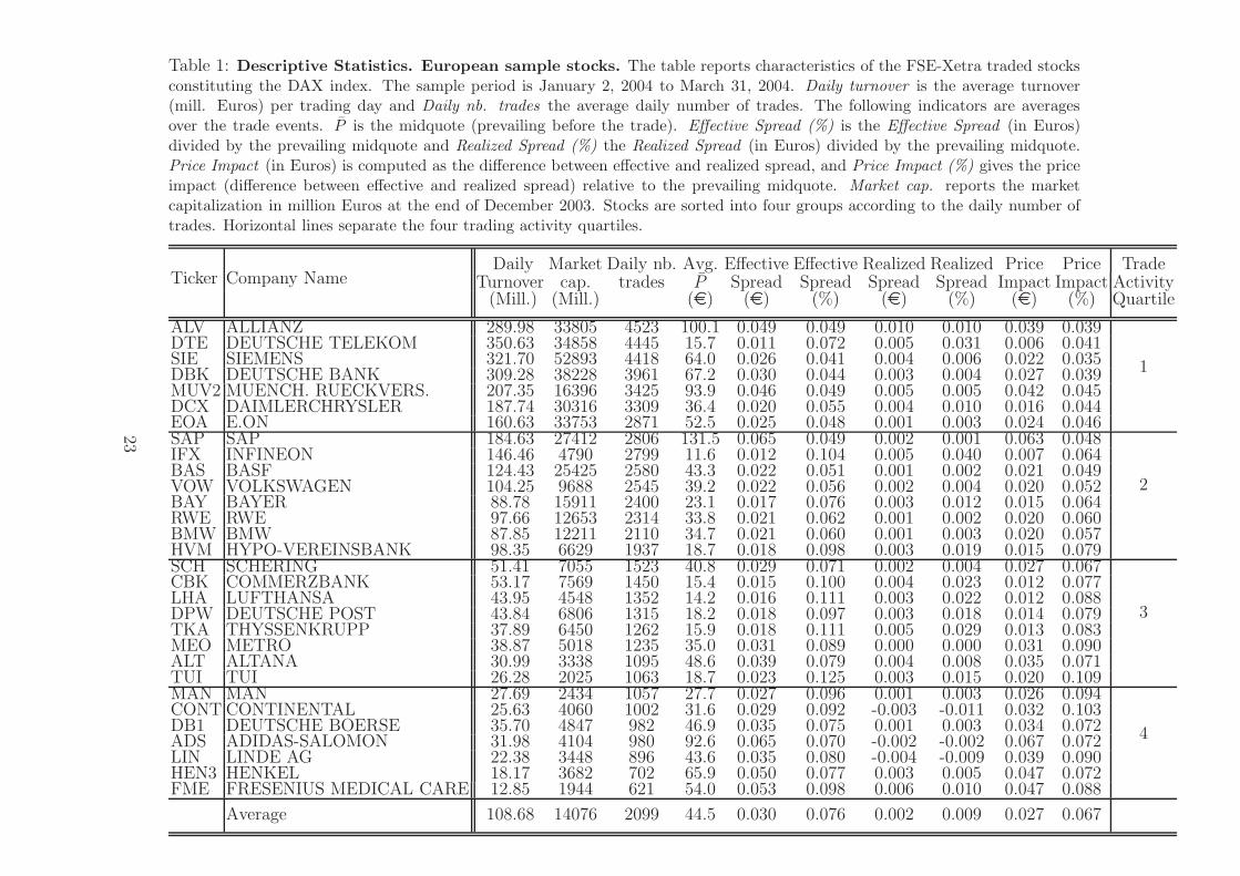
Table 1: Descriptive Statistics. European sample stocks. The table reports characteristics of the FSE-Xetra traded stocksconstituting the DAX index. The sample period is January 2, 2004 to March 31, 2004. Daily turnover is the average turnover(mill. Euros) per trading day and Daily nb. trades the average daily number of trades. The following indicators are averagesover the trade events. P is the midquote (prevailing before the trade). Effective Spread (%) is the Effective Spread (in Euros)divided by the prevailing midquote and Realized Spread (%) the Realized Spread (in Euros) divided by the prevailing midquote.Price Impact (in Euros) is computed as the difference between effective and realized spread, and Price Impact (%) gives the priceimpact (difference between effective and realized spread) relative to the prevailing midquote. Market cap. reports the marketcapitalization in million Euros at the end of December 2003. Stocks are sorted into four groups according to the daily number oftrades. Horizontal lines separate the four trading activity quartiles.
Ticker Company NameDaily Market Daily nb. Avg. Effective Effective Realized Realized Price Price Trade
Turnover cap. trades P Spread Spread Spread Spread Impact Impact Activity(Mill.) (Mill.) (e) (e) (%) (e) (%) (e) (%) Quartile
ALV ALLIANZ 289.98 33805 4523 100.1 0.049 0.049 0.010 0.010 0.039 0.039
1
DTE DEUTSCHE TELEKOM 350.63 34858 4445 15.7 0.011 0.072 0.005 0.031 0.006 0.041SIE SIEMENS 321.70 52893 4418 64.0 0.026 0.041 0.004 0.006 0.022 0.035DBK DEUTSCHE BANK 309.28 38228 3961 67.2 0.030 0.044 0.003 0.004 0.027 0.039MUV2 MUENCH. RUECKVERS. 207.35 16396 3425 93.9 0.046 0.049 0.005 0.005 0.042 0.045DCX DAIMLERCHRYSLER 187.74 30316 3309 36.4 0.020 0.055 0.004 0.010 0.016 0.044EOA E.ON 160.63 33753 2871 52.5 0.025 0.048 0.001 0.003 0.024 0.046SAP SAP 184.63 27412 2806 131.5 0.065 0.049 0.002 0.001 0.063 0.048
2
IFX INFINEON 146.46 4790 2799 11.6 0.012 0.104 0.005 0.040 0.007 0.064BAS BASF 124.43 25425 2580 43.3 0.022 0.051 0.001 0.002 0.021 0.049VOW VOLKSWAGEN 104.25 9688 2545 39.2 0.022 0.056 0.002 0.004 0.020 0.052BAY BAYER 88.78 15911 2400 23.1 0.017 0.076 0.003 0.012 0.015 0.064RWE RWE 97.66 12653 2314 33.8 0.021 0.062 0.001 0.002 0.020 0.060BMW BMW 87.85 12211 2110 34.7 0.021 0.060 0.001 0.003 0.020 0.057HVM HYPO-VEREINSBANK 98.35 6629 1937 18.7 0.018 0.098 0.003 0.019 0.015 0.079SCH SCHERING 51.41 7055 1523 40.8 0.029 0.071 0.002 0.004 0.027 0.067
3
CBK COMMERZBANK 53.17 7569 1450 15.4 0.015 0.100 0.004 0.023 0.012 0.077LHA LUFTHANSA 43.95 4548 1352 14.2 0.016 0.111 0.003 0.022 0.012 0.088DPW DEUTSCHE POST 43.84 6806 1315 18.2 0.018 0.097 0.003 0.018 0.014 0.079TKA THYSSENKRUPP 37.89 6450 1262 15.9 0.018 0.111 0.005 0.029 0.013 0.083MEO METRO 38.87 5018 1235 35.0 0.031 0.089 0.000 0.000 0.031 0.090ALT ALTANA 30.99 3338 1095 48.6 0.039 0.079 0.004 0.008 0.035 0.071TUI TUI 26.28 2025 1063 18.7 0.023 0.125 0.003 0.015 0.020 0.109MAN MAN 27.69 2434 1057 27.7 0.027 0.096 0.001 0.003 0.026 0.094
4
CONT CONTINENTAL 25.63 4060 1002 31.6 0.029 0.092 -0.003 -0.011 0.032 0.103DB1 DEUTSCHE BOERSE 35.70 4847 982 46.9 0.035 0.075 0.001 0.003 0.034 0.072ADS ADIDAS-SALOMON 31.98 4104 980 92.6 0.065 0.070 -0.002 -0.002 0.067 0.072LIN LINDE AG 22.38 3448 896 43.6 0.035 0.080 -0.004 -0.009 0.039 0.090HEN3 HENKEL 18.17 3682 702 65.9 0.050 0.077 0.003 0.005 0.047 0.072FME FRESENIUS MEDICAL CARE 12.85 1944 621 54.0 0.053 0.098 0.006 0.010 0.047 0.088
Average 108.68 14076 2099 44.5 0.030 0.076 0.002 0.009 0.027 0.067
23
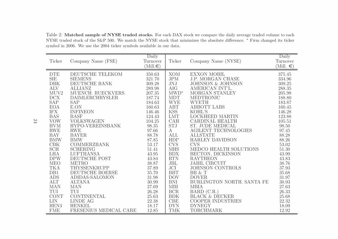
Table 2: Matched sample of NYSE traded stocks. For each DAX stock we compare the daily average traded volume to eachNYSE traded stock of the S&P 500. We match the NYSE stock that minimizes the absolute difference. ∗ Firm changed its tickersymbol in 2006. We use the 2004 ticker symbols available in our data.
Daily DailyTicker Company Name (FSE) Turnover Ticker Company Name (NYSE) Turnover
(Mill.e) (Mill. e)
DTE DEUTSCHE TELEKOM 350.63 XOM EXXON MOBIL 375.45SIE SIEMENS 321.70 JPM J.P. MORGAN CHASE 334.96DBK DEUTSCHE BANK 309.28 JNJ JOHNSON & JOHNSON 309.25ALV ALLIANZ 289.98 AIG AMERICAN INT’L. 288.35MUV2 MUENCH. RUECKVERS. 207.35 MWD∗ MORGAN STANLEY 205.98DCX DAIMLERCHRYSLER 187.74 MDT MEDTRONIC 188.80SAP SAP 184.63 WYE WYETH 183.87EOA E.ON 160.63 ABT ABBOTT LABS 160.45IFX INFINEON 146.46 KSS KOHL’S 146.28BAS BASF 124.43 LMT LOCKHEED MARTIN 123.88VOW VOLKSWAGEN 104.25 CAH CARDINAL HEALTH 105.51HVM HYPO-VEREINSBANK 98.35 STJ ST. JUDE MEDICAL 98.50RWE RWE 97.66 A AGILENT TECHNOLOGIES 97.45BAY BAYER 88.78 ALL ALLSTATE 88.28BMW BMW 87.85 HDI∗ HARLEY DAVIDSON 88.26CBK COMMERZBANK 53.17 CVS CVS 53.02SCH SCHERING 51.41 MHS MEDCO HEALTH SOLUTIONS 51.30LHA LUFTHANSA 43.95 BDX BECTON, DICKINSON 43.99DPW DEUTSCHE POST 43.84 RTN RAYTHEON 43.83MEO METRO 38.87 JBL JABIL CIRCUIT 38.76TKA THYSSENKRUPP 37.89 JCI JOHNSON CONTROLS 37.93DB1 DEUTSCHE BOERSE 35.70 BBT BB & T 35.68ADS ADIDAS-SALOMON 31.98 DOV DOVER 31.97ALT ALTANA 30.99 BNI BURLINGTON NORTH. SANTA FE 30.93MAN MAN 27.69 MBI MBIA 27.63TUI TUI 26.28 BCR BARD (C.R.) 26.33CONT CONTINENTAL 25.63 BDK BLACK & DECKER 25.68LIN LINDE AG 22.38 CBE COOPER INDUSTRIES 22.32HEN3 HENKEL 18.17 DYN DYNEGY 18.09FME FRESENIUS MEDICAL CARE 12.85 TMK TORCHMARK 12.92
24
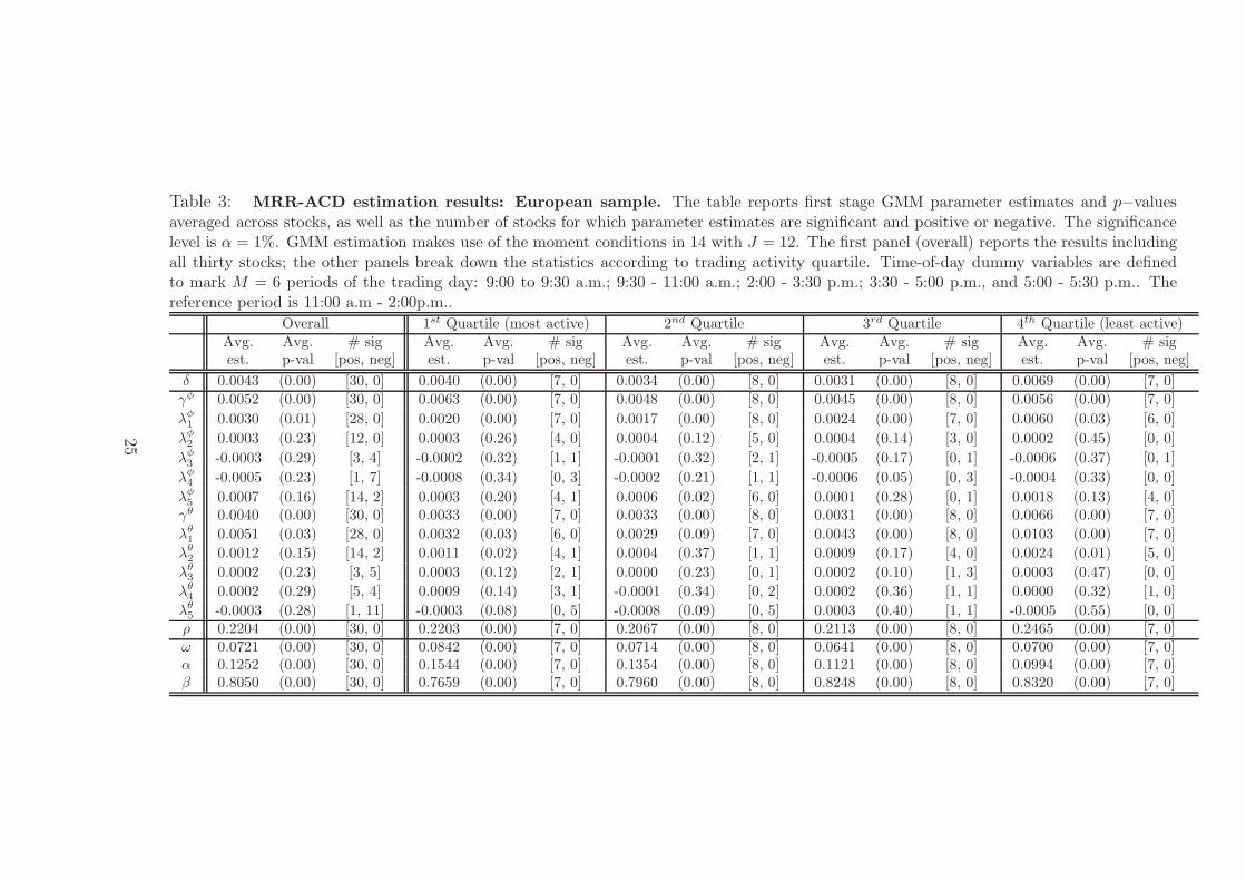
Table 3: MRR-ACD estimation results: European sample. The table reports first stage GMM parameter estimates and p−valuesaveraged across stocks, as well as the number of stocks for which parameter estimates are significant and positive or negative. The significancelevel is α = 1%. GMM estimation makes use of the moment conditions in 14 with J = 12. The first panel (overall) reports the results includingall thirty stocks; the other panels break down the statistics according to trading activity quartile. Time-of-day dummy variables are definedto mark M = 6 periods of the trading day: 9:00 to 9:30 a.m.; 9:30 - 11:00 a.m.; 2:00 - 3:30 p.m.; 3:30 - 5:00 p.m., and 5:00 - 5:30 p.m.. Thereference period is 11:00 a.m - 2:00p.m..
Overall 1st Quartile (most active) 2nd Quartile 3rd Quartile 4th Quartile (least active)Avg. Avg. # sig Avg. Avg. # sig Avg. Avg. # sig Avg. Avg. # sig Avg. Avg. # sigest. p-val [pos, neg] est. p-val [pos, neg] est. p-val [pos, neg] est. p-val [pos, neg] est. p-val [pos, neg]
δ 0.0043 (0.00) [30, 0] 0.0040 (0.00) [7, 0] 0.0034 (0.00) [8, 0] 0.0031 (0.00) [8, 0] 0.0069 (0.00) [7, 0]
γφ 0.0052 (0.00) [30, 0] 0.0063 (0.00) [7, 0] 0.0048 (0.00) [8, 0] 0.0045 (0.00) [8, 0] 0.0056 (0.00) [7, 0]
λφ1
0.0030 (0.01) [28, 0] 0.0020 (0.00) [7, 0] 0.0017 (0.00) [8, 0] 0.0024 (0.00) [7, 0] 0.0060 (0.03) [6, 0]
λφ2
0.0003 (0.23) [12, 0] 0.0003 (0.26) [4, 0] 0.0004 (0.12) [5, 0] 0.0004 (0.14) [3, 0] 0.0002 (0.45) [0, 0]
λφ3
-0.0003 (0.29) [3, 4] -0.0002 (0.32) [1, 1] -0.0001 (0.32) [2, 1] -0.0005 (0.17) [0, 1] -0.0006 (0.37) [0, 1]
λφ4
-0.0005 (0.23) [1, 7] -0.0008 (0.34) [0, 3] -0.0002 (0.21) [1, 1] -0.0006 (0.05) [0, 3] -0.0004 (0.33) [0, 0]
λφ5
0.0007 (0.16) [14, 2] 0.0003 (0.20) [4, 1] 0.0006 (0.02) [6, 0] 0.0001 (0.28) [0, 1] 0.0018 (0.13) [4, 0]γθ 0.0040 (0.00) [30, 0] 0.0033 (0.00) [7, 0] 0.0033 (0.00) [8, 0] 0.0031 (0.00) [8, 0] 0.0066 (0.00) [7, 0]
λθ1
0.0051 (0.03) [28, 0] 0.0032 (0.03) [6, 0] 0.0029 (0.09) [7, 0] 0.0043 (0.00) [8, 0] 0.0103 (0.00) [7, 0]
λθ2
0.0012 (0.15) [14, 2] 0.0011 (0.02) [4, 1] 0.0004 (0.37) [1, 1] 0.0009 (0.17) [4, 0] 0.0024 (0.01) [5, 0]
λθ3 0.0002 (0.23) [3, 5] 0.0003 (0.12) [2, 1] 0.0000 (0.23) [0, 1] 0.0002 (0.10) [1, 3] 0.0003 (0.47) [0, 0]
λθ4
0.0002 (0.29) [5, 4] 0.0009 (0.14) [3, 1] -0.0001 (0.34) [0, 2] 0.0002 (0.36) [1, 1] 0.0000 (0.32) [1, 0]
λθ5 -0.0003 (0.28) [1, 11] -0.0003 (0.08) [0, 5] -0.0008 (0.09) [0, 5] 0.0003 (0.40) [1, 1] -0.0005 (0.55) [0, 0]ρ 0.2204 (0.00) [30, 0] 0.2203 (0.00) [7, 0] 0.2067 (0.00) [8, 0] 0.2113 (0.00) [8, 0] 0.2465 (0.00) [7, 0]ω 0.0721 (0.00) [30, 0] 0.0842 (0.00) [7, 0] 0.0714 (0.00) [8, 0] 0.0641 (0.00) [8, 0] 0.0700 (0.00) [7, 0]α 0.1252 (0.00) [30, 0] 0.1544 (0.00) [7, 0] 0.1354 (0.00) [8, 0] 0.1121 (0.00) [8, 0] 0.0994 (0.00) [7, 0]β 0.8050 (0.00) [30, 0] 0.7659 (0.00) [7, 0] 0.7960 (0.00) [8, 0] 0.8248 (0.00) [8, 0] 0.8320 (0.00) [7, 0]
25
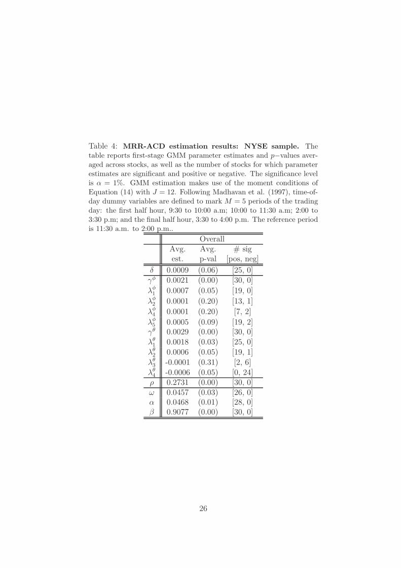
Table 4: MRR-ACD estimation results: NYSE sample. Thetable reports first-stage GMM parameter estimates and p−values aver-aged across stocks, as well as the number of stocks for which parameterestimates are significant and positive or negative. The significance levelis α = 1%. GMM estimation makes use of the moment conditions ofEquation (14) with J = 12. Following Madhavan et al. (1997), time-of-day dummy variables are defined to mark M = 5 periods of the tradingday: the first half hour, 9:30 to 10:00 a.m; 10:00 to 11:30 a.m; 2:00 to3:30 p.m; and the final half hour, 3:30 to 4:00 p.m. The reference periodis 11:30 a.m. to 2:00 p.m..
OverallAvg. Avg. # sigest. p-val [pos, neg]
δ 0.0009 (0.06) [25, 0]γφ 0.0021 (0.00) [30, 0]
λφ1 0.0007 (0.05) [19, 0]
λφ2 0.0001 (0.20) [13, 1]
λφ4 0.0001 (0.20) [7, 2]
λφ5 0.0005 (0.09) [19, 2]γθ 0.0029 (0.00) [30, 0]
λθ1 0.0018 (0.03) [25, 0]
λθ2 0.0006 (0.05) [19, 1]
λθ3 -0.0001 (0.31) [2, 6]
λθ4 -0.0006 (0.05) [0, 24]ρ 0.2731 (0.00) [30, 0]ω 0.0457 (0.03) [26, 0]α 0.0468 (0.01) [28, 0]β 0.9077 (0.00) [30, 0]
26
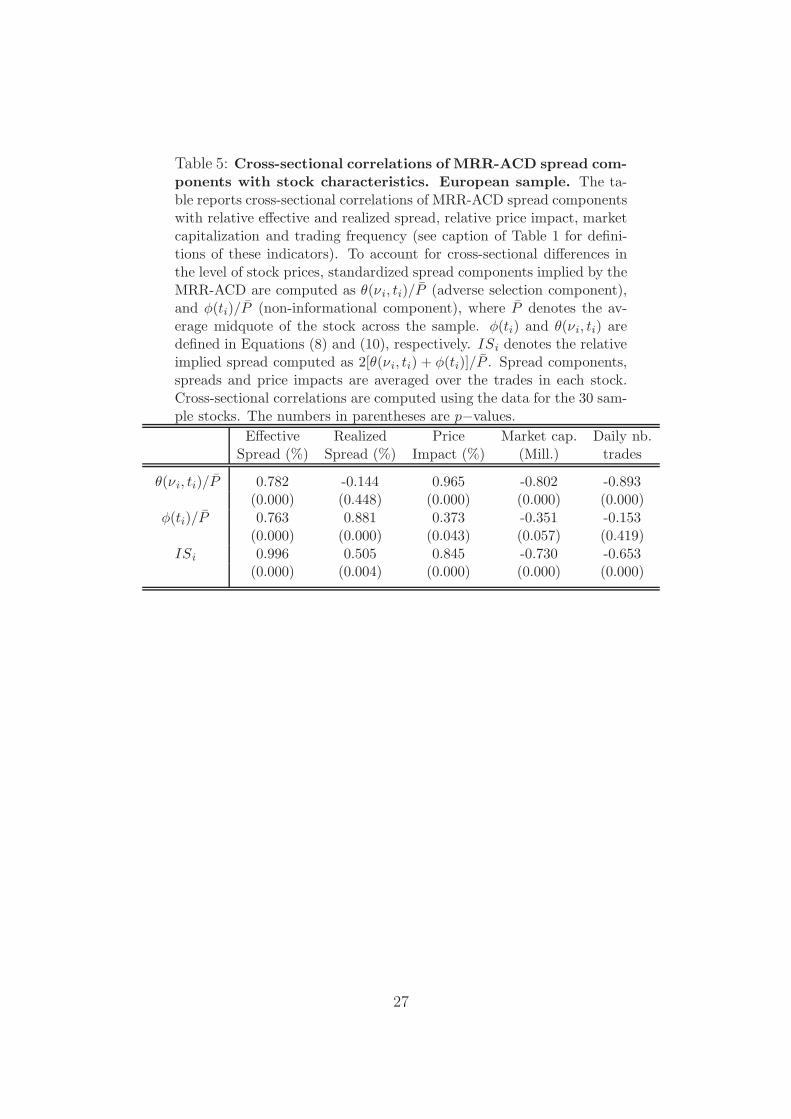
Table 5: Cross-sectional correlations of MRR-ACD spread com-ponents with stock characteristics. European sample. The ta-ble reports cross-sectional correlations of MRR-ACD spread componentswith relative effective and realized spread, relative price impact, marketcapitalization and trading frequency (see caption of Table 1 for defini-tions of these indicators). To account for cross-sectional differences inthe level of stock prices, standardized spread components implied by theMRR-ACD are computed as θ(νi, ti)/P (adverse selection component),and φ(ti)/P (non-informational component), where P denotes the av-erage midquote of the stock across the sample. φ(ti) and θ(νi, ti) aredefined in Equations (8) and (10), respectively. ISi denotes the relativeimplied spread computed as 2[θ(νi, ti) + φ(ti)]/P . Spread components,spreads and price impacts are averaged over the trades in each stock.Cross-sectional correlations are computed using the data for the 30 sam-ple stocks. The numbers in parentheses are p−values.
Effective Realized Price Market cap. Daily nb.Spread (%) Spread (%) Impact (%) (Mill.) trades
θ(νi, ti)/P 0.782 -0.144 0.965 -0.802 -0.893(0.000) (0.448) (0.000) (0.000) (0.000)
φ(ti)/P 0.763 0.881 0.373 -0.351 -0.153(0.000) (0.000) (0.043) (0.057) (0.419)
ISi 0.996 0.505 0.845 -0.730 -0.653(0.000) (0.004) (0.000) (0.000) (0.000)
27
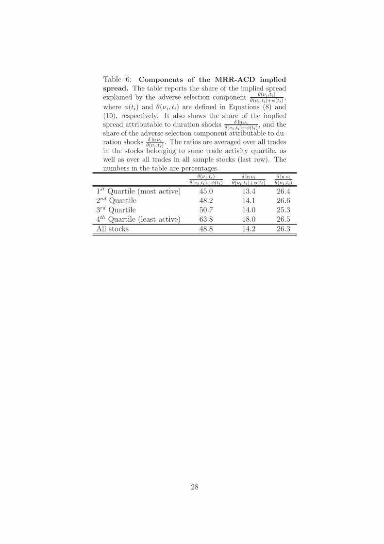
Table 6: Components of the MRR-ACD impliedspread. The table reports the share of the implied spreadexplained by the adverse selection component θ(νi,ti)
θ(νi,ti)+φ(ti),
where φ(ti) and θ(νi, ti) are defined in Equations (8) and(10), respectively. It also shows the share of the impliedspread attributable to duration shocks δ ln νi
θ(νi,ti)+φ(ti), and the
share of the adverse selection component attributable to du-ration shocks δ ln νi
θ(νi,ti). The ratios are averaged over all trades
in the stocks belonging to same trade activity quartile, aswell as over all trades in all sample stocks (last row). Thenumbers in the table are percentages.
θ(νi,ti)θ(νi,ti)+φ(ti)
δ ln νiθ(νi,ti)+φ(ti)
δ ln νiθ(νi,ti)
1st Quartile (most active) 45.0 13.4 26.42nd Quartile 48.2 14.1 26.63rd Quartile 50.7 14.0 25.34th Quartile (least active) 63.8 18.0 26.5All stocks 48.8 14.2 26.3
28
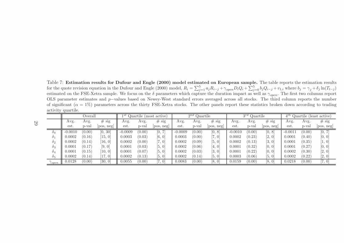
Table 7: Estimation results for Dufour and Engle (2000) model estimated on European sample. The table reports the estimation resultsfor the quote revision equation in the Dufour and Engle (2000) model, Ri =
∑5j=1 ajRi−j +γopenDiQi+
∑5j=0 bjQi−j +v1,i where bj = γj + δj ln(Tt−j)
estimated on the FSE-Xetra sample. We focus on the δ parameters which capture the duration impact as well as γopen. The first two columns reportOLS parameter estimates and p−values based on Newey-West standard errors averaged across all stocks. The third column reports the numberof significant (α = 1%) parameters across the thirty FSE-Xetra stocks. The other panels report these statistics broken down according to tradingactivity quartile.
Overall 1st Quartile (most active) 2nd Quartile 3rd Quartile 4th Quartile (least active)Avg. Avg. # sig Avg. Avg. # sig Avg. Avg. # sig Avg. Avg. # sig Avg. Avg. # sigest. p-val [pos, neg] est. p-val [pos, neg] est. p-val [pos, neg] est. p-val [pos, neg] est. p-val [pos, neg]
δ0 -0.0010 (0.00) [0, 30] -0.0009 (0.00) [0, 7] -0.0009 (0.00) [0, 8] -0.0010 (0.00) [0, 8] -0.0011 (0.00) [0, 7]δ1 0.0002 (0.16) [15, 0] 0.0003 (0.03) [6, 0] 0.0003 (0.00) [7, 0] 0.0002 (0.23) [2, 0] 0.0001 (0.40) [0, 0]δ2 0.0002 (0.14) [16, 0] 0.0002 (0.00) [7, 0] 0.0002 (0.09) [5, 0] 0.0002 (0.13) [3, 0] 0.0001 (0.35) [1, 0]δ3 0.0001 (0.17) [9, 0] 0.0001 (0.03) [5, 0] 0.0002 (0.06) [4, 0] 0.0001 (0.32) [0, 0] 0.0001 (0.27) [0, 0]δ4 0.0001 (0.15) [10, 0] 0.0001 (0.07) [5, 0] 0.0002 (0.03) [3, 0] 0.0001 (0.22) [0, 0] 0.0002 (0.30) [2, 0]δ5 0.0002 (0.14) [17, 0] 0.0002 (0.13) [5, 0] 0.0002 (0.14) [5, 0] 0.0003 (0.06) [5, 0] 0.0002 (0.22) [2, 0]
γopen 0.0128 (0.00) [30, 0] 0.0055 (0.00) [7, 0] 0.0083 (0.00) [8, 0] 0.0159 (0.00) [8, 0] 0.0218 (0.00) [7, 0]
29

Table 8: Effect of three trades on midquote (MQ) and transaction prices (P )
t0 t1 t2 t3initial state small buyer-
initiated trade(P=105)
market-to-limitbuy order withlimit priceP = 105 takesbest ask andimproves the bestbid
remaining vol-ume of MLOconsumed byseller-initiatedtrade (P = 105)
2nd ask 110 110best ask 105 105 110 110MQ 102.5 102.5 107.5 105best bid 100 100 105 1002nd bid 90 90 100 903rd bid 90
∆ MQ 0 4.9% -2.3%
∆P 0 0 0
30
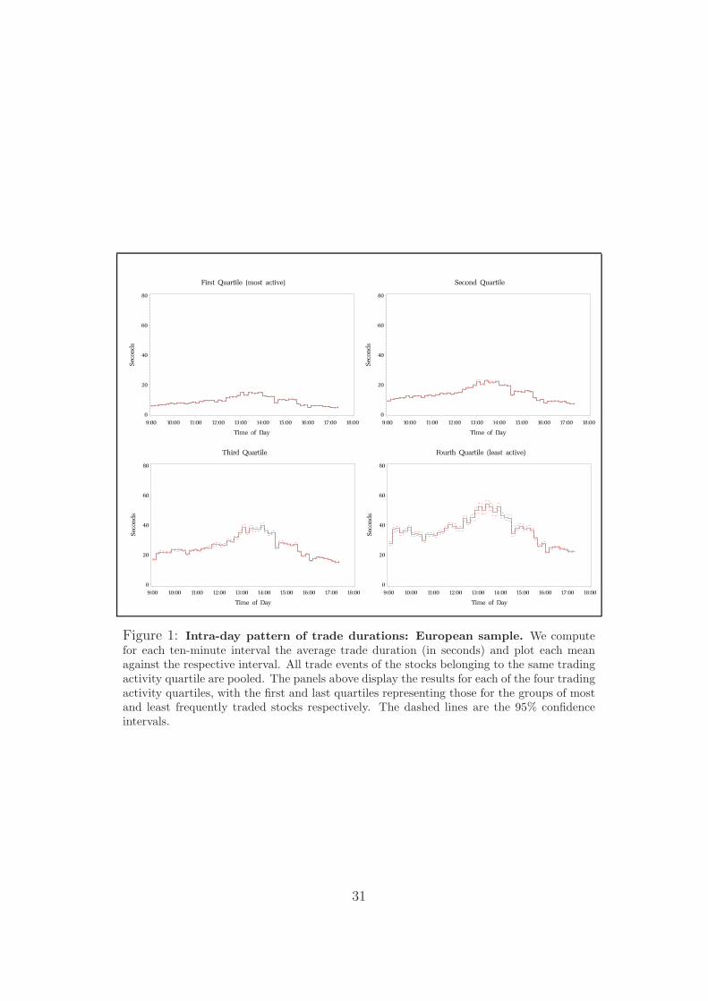
Figure 1: Intra-day pattern of trade durations: European sample. We computefor each ten-minute interval the average trade duration (in seconds) and plot each meanagainst the respective interval. All trade events of the stocks belonging to the same tradingactivity quartile are pooled. The panels above display the results for each of the four tradingactivity quartiles, with the first and last quartiles representing those for the groups of mostand least frequently traded stocks respectively. The dashed lines are the 95% confidenceintervals.
31
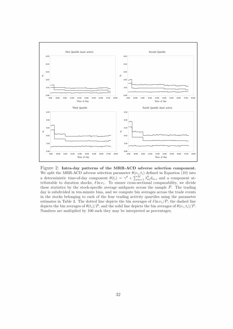
Figure 2: Intra-day patterns of the MRR-ACD adverse selection component.We split the MRR-ACD adverse selection parameter θ(νi, ti) defined in Equation (10) into
a deterministic time-of-day component θ(ti) = γθ +∑M
m=1λθmdm,i and a component at-
tributable to duration shocks, δ ln νi. To ensure cross-sectional comparability, we dividethese statistics by the stock-specific average midquote across the sample P . The tradingday is subdivided in ten-minute bins, and we compute bin averages across the trade eventsin the stocks belonging to each of the four trading activity quartiles using the parameterestimates in Table 3. The dotted line depicts the bin averages of δ ln νi/P ; the dashed linedepicts the bin averages of θ(ti)/P , and the solid line depicts the bin averages of θ(νi, ti)/P .Numbers are multiplied by 100 such they may be interpreted as percentages.
32
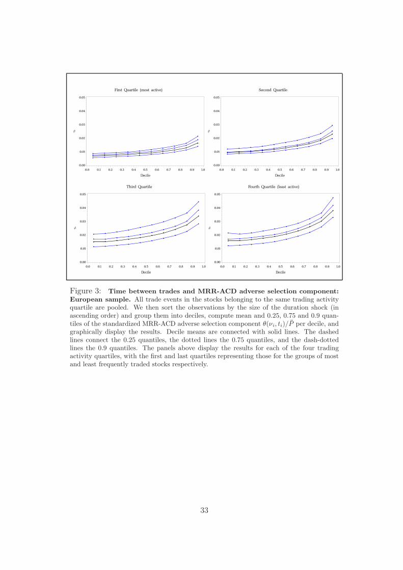
Figure 3: Time between trades and MRR-ACD adverse selection component:European sample. All trade events in the stocks belonging to the same trading activityquartile are pooled. We then sort the observations by the size of the duration shock (inascending order) and group them into deciles, compute mean and 0.25, 0.75 and 0.9 quan-tiles of the standardized MRR-ACD adverse selection component θ(νi, ti)/P per decile, andgraphically display the results. Decile means are connected with solid lines. The dashedlines connect the 0.25 quantiles, the dotted lines the 0.75 quantiles, and the dash-dottedlines the 0.9 quantiles. The panels above display the results for each of the four tradingactivity quartiles, with the first and last quartiles representing those for the groups of mostand least frequently traded stocks respectively.
33
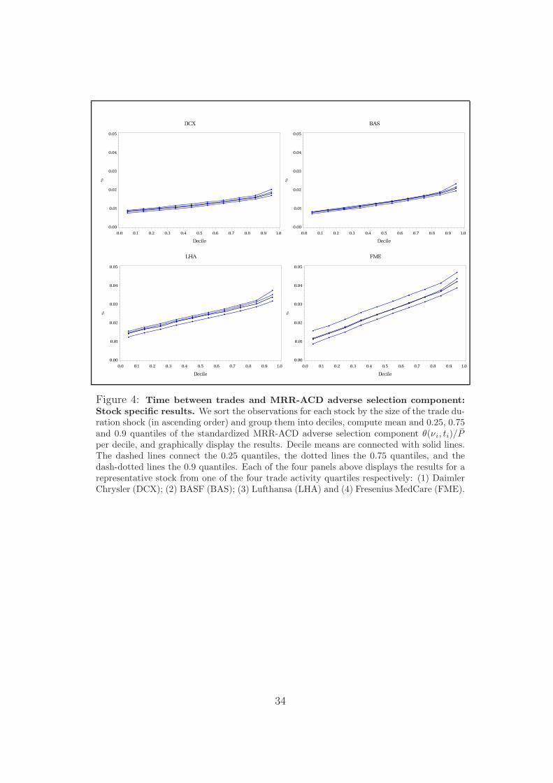
Figure 4: Time between trades and MRR-ACD adverse selection component:Stock specific results. We sort the observations for each stock by the size of the trade du-ration shock (in ascending order) and group them into deciles, compute mean and 0.25, 0.75and 0.9 quantiles of the standardized MRR-ACD adverse selection component θ(νi, ti)/Pper decile, and graphically display the results. Decile means are connected with solid lines.The dashed lines connect the 0.25 quantiles, the dotted lines the 0.75 quantiles, and thedash-dotted lines the 0.9 quantiles. Each of the four panels above displays the results for arepresentative stock from one of the four trade activity quartiles respectively: (1) DaimlerChrysler (DCX); (2) BASF (BAS); (3) Lufthansa (LHA) and (4) Fresenius MedCare (FME).
34
CFS Working Paper Series: No. Author(s) Title
2011/07 Tullio Jappelli Mario Padula
Investment in Financial Literacy and Saving Decisions
2011/06 Carolina Achury Sylwia Hubar Christos Koulovatianos
Saving Rates and Portfolio Choice with Subsistence Consumption
2011/05 Gerlinde Fellner Erik Theissen
Short Sale Constraints, Divergence of Opinion and Asset Values: Evidence from the Laboratory
2011/04 André Betzer Jasmin Gider Daniel Metzger Erik Theissen
Strategic Trading and Trade Reporting by Corporate Insiders
2011/03 Joachim Grammig Eric Theissen
Is BEST Really Better? Internalization of Orders in an Open Limit Order Book
2011/02 Jördis Hengelbrock Eric Theissen Christian Westheide
Market Response to Investor Sentiment
2011/01 Mathias Hoffmann Michael U. Krause Thomas Laubach
Long-run Growth Expectations and "Global Imbalances"
2010/26 Ester Faia Credit Risk Transfers and the Macroeconomy
2010/25 Ignazio Angeloni Ester Faia Roland Winkler
Exit Strategies
2010/24 Roman Kräussl Andre Lucas Arjen Siegmann
Risk Aversion under Preference Uncertainty
Copies of working papers can be downloaded at http://www.ifk-cfs.de