SLAC-PUB-2070 January, 1978 CT)

LAZTICE MODELS OF QUARK CONFINEMENT AT HIGH TEMPERATURE

Leonard Susskind Stanford Linear Accelerator Center

Stanford University, Stanford, California 94305

and

Tel Aviv University Ramat Aviv Israel

ABSTRACT

We consider the behavior of lattice models of quark confinement at high tem-

perature. We find that confinement is strictly a low temperature phenomenon.

At high temperatures a transition to a plasma-like phase occurs, In this phase

free gluons form a plasma which Debye screens the quarks. .

(Submitted to Phys. Rev. D. )

*Work supported in part by the Department of Energy.

-2-

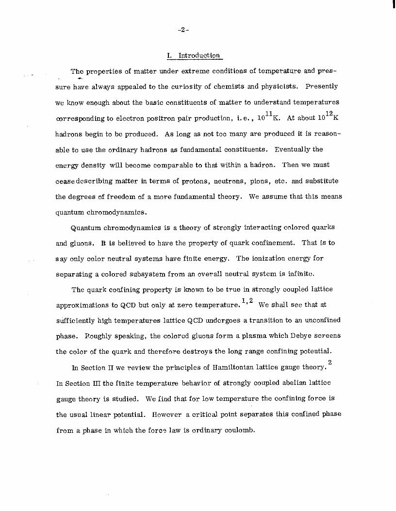
1. Introduction

The properties of matter under extreme conditions of temperature and pres- 4

sure have always appealed to the curiosity of chemists and physicists. Presently

we know enough about the basic constituents of matter to understand temperatures

corresponding to electron positron pair production, i. e. , 10 11 K. At about 10 12 K

hadrons begin to be produced. As long as not too many are produced it is reason-

able to use the ordinary hadrons as fundamental constituents. Eventually the

energy density will become comparable to that within a hadron. Then we must

cease describing matter in terms of protons, neutrons, pions, etc. and substitute

the degrees of freedom of a more fundamental theory. We assume that this means

quantum chromodynamics.

Quantum chromodynamics is a theory of strongly interacting colored quarks

and gluons. It is believed to have the property of quark confinement. That is to

say only color neutral systems have finite energy. The ionization energy for

separating a colored subsystem from an overall neutral system is infinite.

The quark confining property is known to be true in strongly coupled lattice

approximations to QCD but only at zero temperature. 192 We shall see that at

sufficiently high temperatures lattice QCD undergoes a transition to an unconfined

phase. R.oughly speaking, the colored gluons form a plasma which Debye screens

the color of the quark and therefore destroys the long range confining potential.

In Section II we review the principles of Hamiltonian lattice gauge theory. 2

In Section III the finite temperature behavior of strongly coupled abelian lattice

gauge theory is studied. We find that for low temperature the confining force is

the usual linear potential. However a critical point separates this confined phase

from a phase in which the force law is ordinary coulomb.

-3-

In Section IV we continue the study of the abelian theory including a charge

carrying field . -

Non-abelian lattice chromodynamics is the subject of Section V. As in the

abelian theory a transition between confined and unconfined phases exists. This

time the unco.nfined phase is characterized by a short range force because the

coulomb force is screened by a plasma of gluons.

The last section discusses the validity of the conclusions for continuum chro-

modynamics.

II. Lattice Gauge Theory

Consider a simple cubic lattice in 3 space dimensions whose sites are

labeled by triplets of integers

r = x, y, z = site

Directed links of the lattice are indicated by a site and one of 6 unit lattice vec- A

tors called tx, n 2 A A A

y9 z9 nBx, ney, nvZ.

(r, t) = link

Each link of the lattice has a degree of freedom V(r, G) which for the abelian

theory is a phase

V= e i@ (Abelian)

For the SUN theory V is a special unitary N dimensional matrix. Each link (r, t)

h as a mate which is just the same link but oppositely oriented. It is the link A A

(r 9 n, -n)

The two degrees of freedom V (r, k) and V(i- + 2, -G) are related

V(r +F;, 4) = Vt(r, k) (1)

For the abelian theory

$(r, t) = -$(r + G, 4) (2)

-4-

In the abelian theory each link carrys an electric flux E(r, 2) which satisfies

-h E(r, $ = -E(r + 2, 4) (3)

[+(r, t), E(r, ;)I= i (4)

E(r, k) is the conjugate momentum to Cp and since @ is an angle E has the integers

for its spectrum

E(r, ‘D) = integer (5)

In the non-abelian theory E is a member of the adjoint representation of

“n’ For our example we will work with SU2 so that E is a 3-vector. It satisfies

[Ea’(r, $, EP(r, G)] = iE olpr Y E (r, 2)

[E”(r, $ EP(rP, iy)] = 0 (r, t) # (r* k”) (6)

Thus the E*s are angular momenta and have the spectrum of integer and l/2 in-

teger angular momenta. The E*s generate left and right group transformations

on the Vps

cEa(r, A), V(r, ?I)] = 7°! V (r, $) (7)

where 7°! are the pauli matrices.

The EPs do not satisfy Eq. (3) but rather

E(r + G, -k) = -V(r, k) E(r, G)VP(r, G)

where

E = EQ?

(8)

(9)

However the E*s do satisfy

E(r, $2 = E(r +fi, -G)2 (10)

In order to express the Hamiltonian we will need a set of operators to iden-

tify with the magnetic field energy. Thus consider an elementary square of the

lattice bounded by the directed links 1, 2, 3, 4 as in Fig. 1.

-5-

We label such a square r and define (abelian theory)

Vu-) = VP) VW VW V(4) &

=e i[4+) + W) + G(3) + (4)]

and (non abelian theory)

TrV(r) = Tr VW VP) VP) v(4)

The Hamiltonian for abelian IGT is

(11)

(12)

(13)

c c where links and Boxes indicate sums over undirected and unoriented links and

boxes. For non abelian L. G. T.

c g2E2 c H=li,nks 2a - Boxes -+ TI(V(I’) + V?(1-)] (14)

ag

The space of states includes unphysical states which are purged by applying

a subsidiary condition. The physic& subspace consists of vectors I+ satisfying

V;-E = ; E(r, @ I$>= 0 all r ( 15)

where c n indicates a sum over the 6 lattice directions. Eq. (15) is the lattice

version of gausses law which says that the total flux leaving a site must equal zero.

It is modified when sources are included.

III. Abelian Gauge Theory at Finite Temperature

We shall argue later that if a transition to an unconfined phase occurs the

transition temperature is bounded from above by ignoring the magnetic tern in

H. In other words if we find a transition to the unconfined phase when H magnetic

is ignored then the full Hamiltonian surely has one at a lower $c. For now we

shall simply work tn the strong coupling approximation in which

c2 A2 H = links za Eh n) (16)

In this approximation confinement is rigorous at zero temperature. 2

-6-

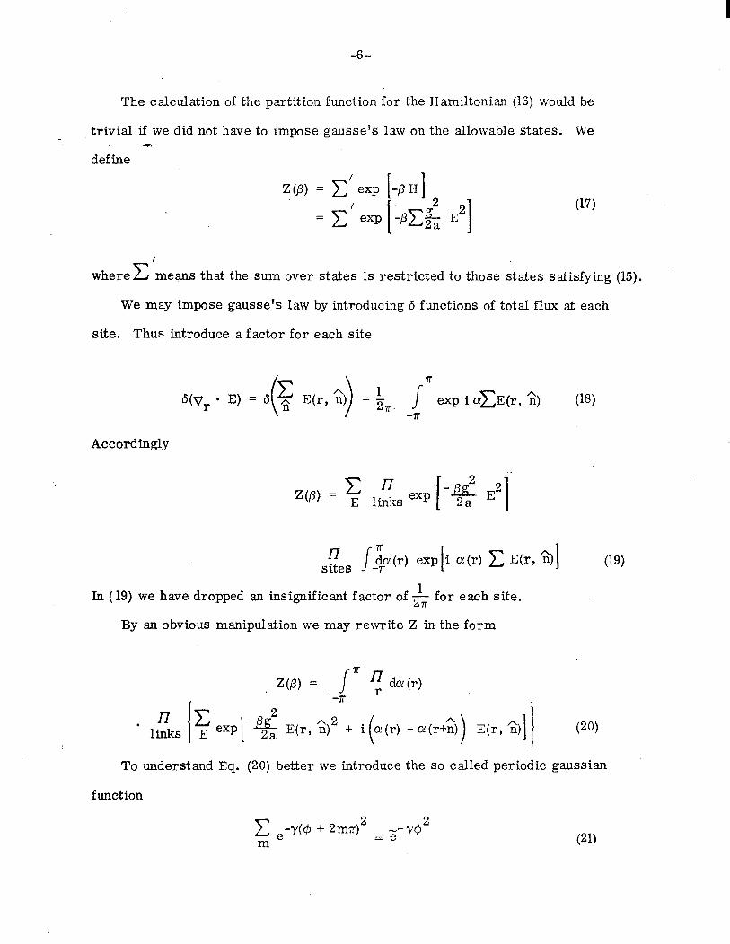
The calculation of the partition function for the Barniltonian (16) would be

trivial if we did not have to impose gausse9s law on the allowable states. We 4\

define

Z(P) = C’ exp I

= c exp

-P H I -Px< E2 I

(17)

I

where c means that the sum over states is restricted to those states satisfying (15).

We may impose gausse’s law by introducing 6 functions of total flux at each

site. Thus introduce a factor for each site

7r Qv, l E) = 6 exp i @xE(r, ^n)

-lr

Accordingly

Z(P) = c E litid exp

n J &!(r) exp sites -7r i o!(r) c E(r, %) 1

In ( 19) we have dropped an insignificant factor of & for each site.

By an obvious manipulation we may rewrite Z in the form

Z(P) = /* y da(r)

l lzs $.exp -Fz E(r $)‘“r+ i I I , - cY(r+GL)

(18)

(19)

(20)

To understand Eq. (20) better we introduce the so called periodic gaussian

function

(21)

-7-

It consists of a periodic super-positron of gaussians and closely resembles

the function 4,

ee2’ exp [2y cos$] (22)

for large y.

To express (20) in terms of periodic gaussians we use the identity

giving

c exp CE2 + iol E E

2,” 7r =

J c ; 4c

(23)

21/2 ’ The numerical factor (27ra/pg ) for each link may be ignored for our pur-

poses. The remaining structure defines the well known Vil1ia.n approximation to

the planar Heisenberg model3 defined by

Z= lRda(r) I7 exp -3 cos a(r) - 01 (r+G) ) -?r links PI3 c I (25)

Note that the usual inverse temperature of the heisenberg magnet is -a/pg2 which

is proportional to the temperature of the original problem. In fact as the temper-

ature of the lattice gauge world increases the effective temperature of the magnetic

model decreases leading to a transition to a magnetized or ordered state.

The Villian model is known to have the following properties: 1) For small

3 the system is disordered. This means Pg

<eiN4 e-is W>y eaplr I r+ao (26)

-8-

2) For large --$, the system is magnetized or ordered. Pg

< eiQ to) .-iQ tr)>wconst. (27)

In fact for very large 5 spin wave analysis shows the correlation to behave like Pg

< e ia (0) e -iol (r)

> [ I E.2

--*’ exp r (28)

Next let us consider the abelian theory with a pair of static charges of mag-

nitude + g at locations r = 0 and r = R. -.These sources are introduced by changing

gausses law to read

c p\ E(r, G) = 0 , r# 0, orR n

\ c E(o, 2) = 1 G

c E(k, ;) = -1 n

(29)

This is implemented by changing the 6 functions in (18) at r = 0 and r = 33.. The

result is to introduce an extra factor of

exp i 01(o) exp -i Q! (R)

into the integrands of (19), (20) and (24). Thus in the presence of sources we

define

Z(p, R) = /’ d a(r)ng-- a [o (r) - 01 (r+n)] 2 -7r 2Pg2

. e ia! (0) .-ia! (R) (30)

= z(pl ce ia (0) ,-ia W>

Now consider the free energy of the system with sources (subtracting the free

energy of the sourceless system).

-9-

w(PR) = - [ln Z(pR) - ln Z(P)]/@

(31)

From Eq. (26) we see that for small temperature

fining and linear

the poten tial is con-

(32)

For high

2 WV, w-:

i. e. a normal coulomb force.

(33)

IV. Abelian Charge Carrying Fields

The existence of charge carrying fields modifies the results of Section III.

The charge carrying field we will use is particularly simple. At each site in-

troduce a phase variable +(I). The complex charge carrying field at site r is

exp i $(r)O The charge in units of g is the cannonical conjugate to $ which we

call Q(r). Q(r) has integer spectrum.

The energy stored in the field Cp will be taken to be

mQ2

where m can be thought of as the mass of a singly charged site. In a more re-

fined model, gauge invariant hopping terms can be added to H to allow the charges

to more through the lattice.

The new model hamiltonian is

H = c 2 E(r, n)2 + m c links 2a

QW2 sites

(34)

and gausse% law must be modified to account for the sources on the sites.

-lO-

‘r - E = Q(r) (35)

The partition function in Eq. (19) is modified in two ways. First the delta

functign is modified to

n) - Q(r)

and secondly we must include the factor

n e -Pm Q2(d

(36)

(37) sites

Thus

Z(P)= c fl E, Q links

exp [- $ E2]

-pm Q2 /” da!(Y) exp,[ia(r)r _ 1 (33)

l I7e E(r, n) sites -7r n

* exp - iol(r) Q(r)

Using Eq. (23) gives

Z(P) =]dW-) I7 links

- 02 (r+n) 2 ‘I 1 2

n N-P a (t-j e 4pm L 1 (39)

sites

This is the Villain approximation to the planar heisenberg model with an

external field .

Z Heisenberg = d 01 fl / exp links

-+- cos al(r) - a!(r+n) Pg 1

*II exp & cos a(r) sites

(40)

-ll-

2 As before, the temperature for the magnetic model in Eq. (40) is 5 which is

inversely proportional to the temperature of the lattice gauge theory. The ex- 4

ternal field is given by & so that in the limit m+ co the charges have no

effect.

The properties of the Villain model in the presence of an external symmetry

breaking field are summarized by the phase diagram in Figure 2.

In Figure 2 the horizontal axis separates states in which the magnetization

M(=cosol) is positive and negative. Along the line between the origin and the

critical point labeled c there is spontaneous magnetization. The magnetization

vanishes on the remainder of the horizontal axis. For various values of h the

magnetization behaves like Figure 3.

For h If 0 the magnetization is a smooth function of % and is always non Pg

zero. The implications of this for the force between external sources is inter-

esting. Eq. (31) still applies. Since =,io!(O) .-ia > must tend to the square

of the magnetization as R ---( co and M does not equal zero for any * (unless Pi?

h= 0) we find that the potential V(R) always tends to a finite limit as R-t cc.

Thus it might seem that there is no confinement of charge even at zero tempera-

ture. This is not the right interpretation as we shall see. But first let us cons&

der the behavior of V(R) for large (R).

In the presence of an external field the correlations in a magnet always be-

have like

1 + c(R) emmR M2

for large R where c(R) falls at most like a power. This gives

W(R) = C(R) eBmR + log M2

(41)

(42)

i.e., a short range yukawa like force law.

-12-

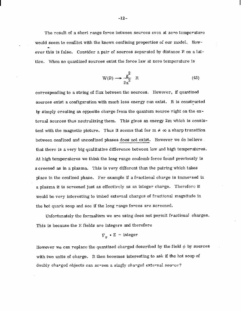
The result of a short range force between sources even at zero temperature

would seem to conflict with the known confining properties of our model. How- 4

ever this is false. Consider a pair of sources separated by distance P on a lat-

tice. When no quantized sources exist the force law at zero temperature is

W(R) + 1 R 2a2

(43)

corresponding to a string of flux between the sources. However, if quantized

sources exist a configuration with much less energy can exist. It is constructed r

by simply creating an opposite charge from the quantum source right on the ex-

ternal sources thus neutralizing them. This gives an energy 2m which is consis-

tent with the magnetic picture. Thus it seems that for m P co a sharp transition

between confined and unconfined phases does not exist. However we do believe

that there is a very big qualitative difference between low and high temperatures.

At high temperatures we think the long range coulomb force found previously is

s creened as in a plasma. This is very different than the pairing which takes

place in the confined phase. For example if a fractional charge is immersed in

a plasma it is screened just as effectively as an integer charge. Therefore it

would be very interesting to imbed external charges of fractional magnitude in

the hot quark soup and see if the long range forces are screened.

Unfortunately the formalism we are using does not permit fractional charges.

This is because the E fields are integers and therefore

v, *E = integer

However we can replace the quantized charged described by the field @ by sources

with two units of charge. It then becomes interesting to ask if the hot soup of

doubly charged objects can scveen a singly charged external source?

-13-

The model Hamiltonian is identical with Eq. (34) but now gausses law becomes

V,sE = 2Q(r) (44)

and Eqs, (39) and (40) are replaced by

C --J$- [CY (7-j - cd (r-f-n)] 2 Z(P) = /da lcks 2 VP 1

1 Pw~12 -- n g 16/3m

sites (45)

Z@) = /da! II e 2 links

a(r) - a(r+n))

I

1 cos2 a(r) n

-I e 2pm I

sites * (46)

Evidently the expression in Eq. (45) is periodic with period 7r instead of 2a.

The symmetry breaking field now has a discrete symmetry

o(r) *a!(r) +7r (47)

at low temperature (high temperature for the Villain-Heisenberg model) this

symmetry is not broken. Thus

< coso!(r)> = 0 (43)

(49)

-14-

The external field does cause

dZl = <cos 2a!(r)) # 0

so that

<e 2ia!(r) .-2i Q(r)> -3 &2 (1 + c e-Clr) w-i

Eqs. (49) and (50) mean that at low temperature singly charged sources experience

linearly forces but doubly charged sources do not. This is consistent with the

usual confinement picture.

At high temperatures (low in H-V model) the system becomes magnetized

M = <cosa> #O (51)

<e ior (0) ,-ia! (r) > - I?(1 + c eBPr) (52)

thus resulting in the screened short range force between singly charged sources.

This type of charge neutralization is entirely different from the pairing of oppo-

site charges to form bound neutral systems. It occurs in plasmas and is called

Debye screening.

V. Non Abelian Theory

For the non abelian theory we consider the model

9

strong coupling Hamiltonian

H = & c ‘Eo(r, n) ECY(r, n) (53) links

supplemented by the constraint

V, - Ea! = xE”!(r, n) Ifi>= 0 (54) ri

The operators c EQ! are algebraically angular momenta. To implement n

Eq. (54) we introduce projection operators at every site which project onto the

zero angular momentum state. These operators are constructed as follows:

-15-

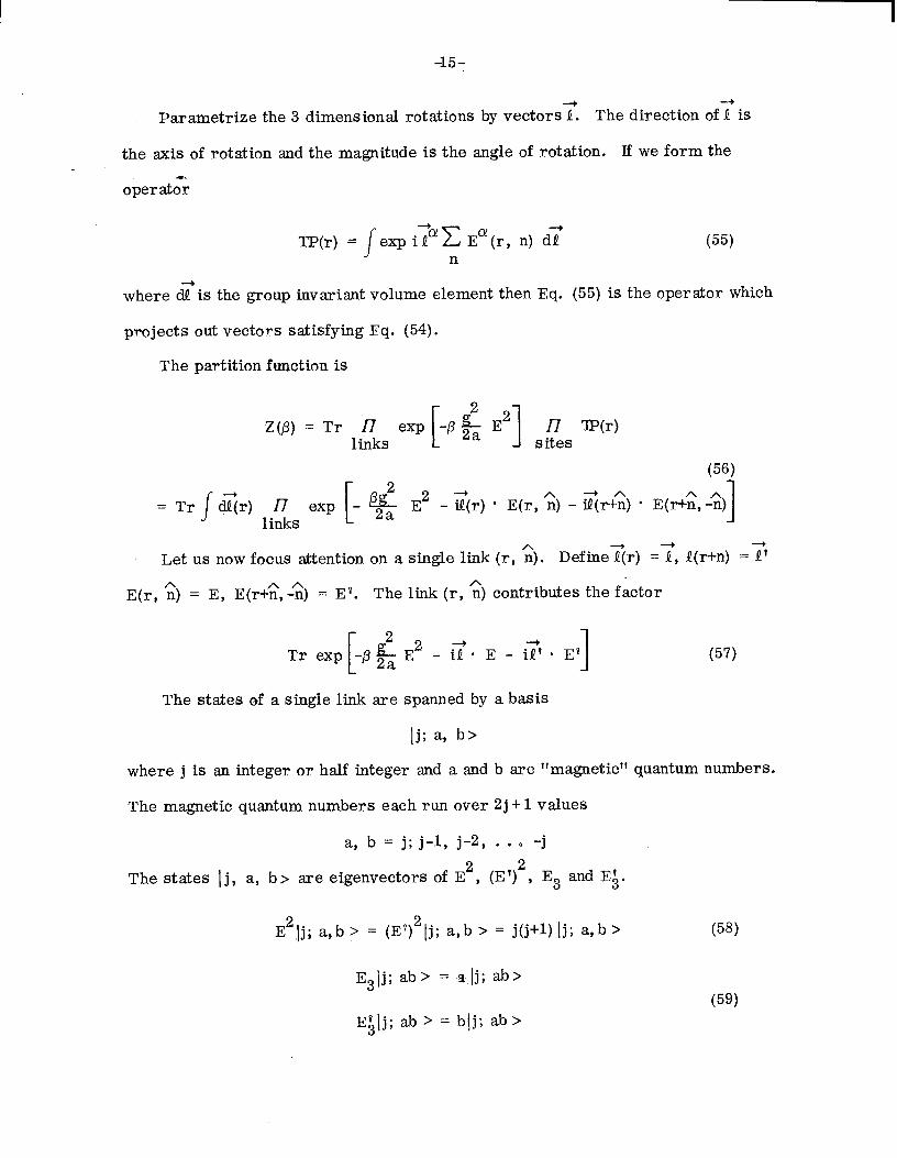
Parametrize the 3 dimensional rotations by vectors7. The direction ofTis

the axis of rotation and the magnitude is the angle of rotation. If we form the

oper at;

YIP(r) = Jexp ipc Eo(r, n) d; n

(55)

where $is the group invariant volume element then Eq. (55) is the operator which

projects out vectors satisfying Fq. (54).

The partition function is

Z(p) = Tr n exp -p [%I E2 l7 w(r) links sites

(55)

= Tr J s(r) n exp - z(r) * E(r, /\n) - ii+;) l E(r&2 links 1

Let us now focus attention on a single link (r, ;). DefineT(r) =T, Q(r+n) =??

E(r, 2) = E, E(r-&,-$) = E*. The link (r, $) contributes the factor

Tr exp E2 - 12. E - i? * E* 1 (57)

The states of a single link are spanned by a basis

lj; a, b>

where j is an integer or half integer and a and b are “magnetic” quantum numbers.

The magnetic quantum numbers each run over 2j + 1 values

a, b = j; j-l, j-2, . . O -j

The states 1 j, a, b> are eigenvectors of E2, (E ‘J2 , E3 and E$.

E’lj; a,b > = (Ev)21j; a,b > = j(j+l) lj; a,b > (53)

E31j; ab> = a Ij; ab> (5%

E$(j; ab > = blj; ab >

-16-

Thus the trace in Eq. (57) is a sum over all integer and l/2 integer j

c, 2 2 c <j; able

+kE _ i7. E _ i; l Et

lj; ab> j,a,b

2 = r . e -p & j - j+l x : (Q) x (1’)

j J .j (60)

where xI is the character of the group element Q.

x, j z) = Tr exp -iT * T. J (61)

where Tj are the angular momentum matrices for spin j. They are easily evalu-

ated

+ X.j(Q) =

sin(j+$Q

sin 2 5

where Q is the angle of rotation (magnitude of;). Thus Eq. (60) becomes

1

Sd

v c ,-!&U+l) sin(j++)Q sin(j++) Q’

2 sin!$ j

The sum can be evaluated in terms of periodic gaussians giving

(62)

(63)

(64)

a Q +Q’ The functions g 2

L ( ) 2 are periodic in QtQ with period 47r. The factor

2 exp p & can be ignored as it will contribute a numerical factor to Z which will

cancel when averages are computed. The factor in brackets will be denoted

-17-

[--$&+r +;-$&+)2](65) F(Q +-Q*, I -Q’) = -e

It is periodic in Q +Q’ with period 47r and is antisymmetric under interchange of

Q-f-Q’ andQ -I ‘. It also has the property of being vanishingly small for large p

unless

Q =Q’

or 1

Q = -Q’

1

The entire partition function can now be written

./- v da(r) sina y n F[Q(r) + Q(r+n), Q(r) - Q(r+n)]

links sin ‘lrl 2 sin Q(r+n)

2

(66)

(67)

The integrations over Q must go from 0 to 4n in order to cover the whole SU2

group space. The factor + is the group-invariant volume element. sm Q/2

Before considering the possible phase transitions which c%an occur, let us con-

sider the partition function in the presence of static sources. The sources are a

pair of SU2 quarks of color l/2. They are described by 7 matrices and have

color operators Ql and Q2. They are located at r =0 and r =R. Thus Gausses

law is modified to

xE(r,/;;) = 0 , r # 0, R n

~E(o, $ = Ql

CEW, 2) = Q2

and the partition function integrand has the extra factors

-18-

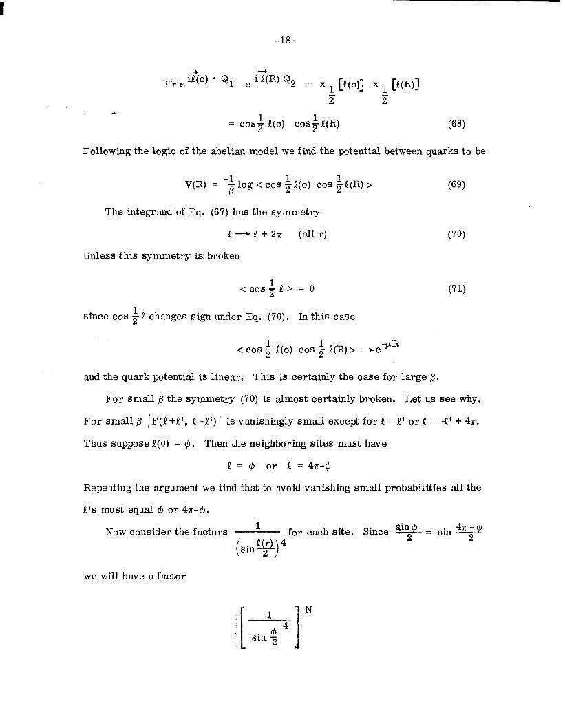
Ty e i;(o) a Ql e iT(R.) Q 2 = x 1 [Q(o)] x 1 [Q(k)]

B 3 4

= cosz ’ Q(o) cos;Q(R) 033)

Following the logic of the abelian model we find the potential between quarks to be

V(R) = -$ log < cos iQ(o) cos 2 La(R) > (69)

The integrand of Eq. (67) has the symmetry

Q--tQ+2~r (allr)

Unless this symmetry is broken

<cos;Q> = 0

since cos +Q changes sign under Eq. (70). In this case

(70)

(71)

< cos $ Q(o) cos f Q(R.)> -9e -PR

and the quark potential is linear. This is certainly the case for large p.

For small p the symmetry (70) is almost certainly broken. Let us see why.

For small p JF(Q+Q~, Q -Q*) 1 is vanishingly small except for Q = 8’ or Q = -Q* + 4n.

Thus suppose Q(0) = $. Then the neighboring sites must have

Q = $ or Q = 4x-4

Repeating the argument we find that to avoid vanishing small probabilities all the

Q*s must equal $ or 47~c$.

Now consider the factors

(sin’ )

for each site. Qfi 4

2

we will have a factor

,,i

1 N

sin s4

-19-

where N is the total number of sites. This means that the values

G M 0 (same as $ = 47r) -

or

are very strongly favored and will dominate the configurations.

The values Q 2 0 and Q NN 27r will not both occur at different sites. The factors

F encorce all the Q*s to be almost the same (mod 4n). We have therefore a con-

ventional spontaneous breaking of symmptry; the broken symmetry being Eq. (70).

We see that in the spontaneously broken states

<co+ +‘ 1

for infinite temperature. Accordingly

< cos ;Q(o) cos f Q(R)> -+M? (1 + c eqR)

and quarks are unconfined,

The mechanism for the short range force undoubtably involves the fact that

the non abelian gauge field can carry color. Thermal fluctuations eventually

cause the colored gluons to form a plasma which Debye screens the quark. 4

VI. Conclusions

We have considered the influence of thermal fluctuations on a particularly

simple model of confinement. The model consists of dropping the magnetic part

of the lattice gauge theory hamiltonian and retaining only the electric terms. Two

questions naturally arise. The first is to what extent the conclusions are modi-

fied when the magnetic terms are included? The second and far more difficult

is whether the phase-transition occurs in the continuum limit.

-2o-

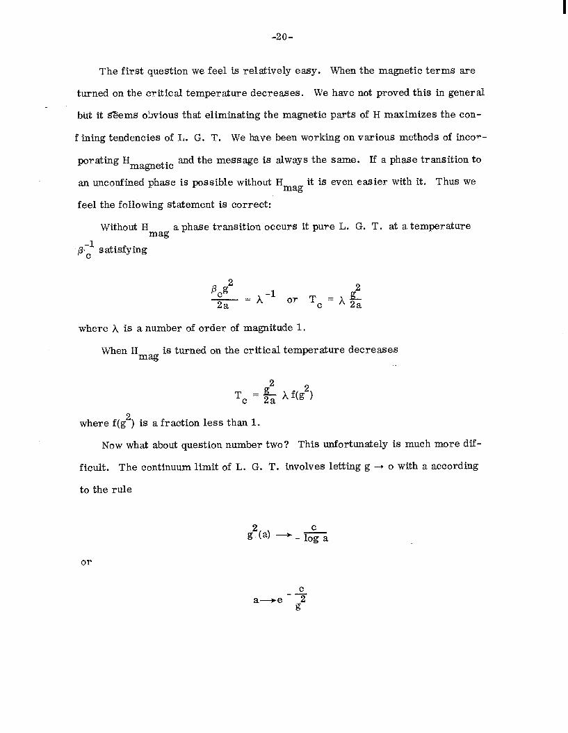
The first question we feel is relatively easy. When the magnetic terms are

turned on the critical temperature decreases. We have not proved this in general

but it &ems obvious that eliminating the magnetic parts of H maximizes the con-

fining tendencies of L. G. T. We have been working on various methods of incor-

porating Hmagnetic and the message is always the same. If a phase transition to

an unconfined phase is possible without H it is even easier with it. Thus we me

feel the following statement is correct:

Without H mag

a phase transition occurs it pure L. G. T. at a temperature

p-,’ satisfying

p,g2 = A-1 2 2a or Tc = k 2a

where A is a number of order of magnitude 1,

When H mag

is turned on the critical temperature decreases

2

Tc =k A f(g2)

where f(g2) is a fraction less than 1.

Now what about question number two? This unfortunately is much more dif-

ficult. The continuum limit of L. G. T. involves letting g -+ o with a according

to the rule

or

C

a-e-- $

-21-

The critical temperature behaves like

*g! e%

= lim g40

+ f(g2)

Thus it is not possible to say with certainty whether the transition occurs in the

limiting theory without knowing the behavior of f(g2) for g2+ o.

Acknowledgments

The authorswishes to thank Eduardo Fradkin for valuable assistance.

REFERENCES

1. K. G. Wilson, Phys. Rev. 10, 2445 (1974).

2. J. Kogut and L. Susskind, Phys. Rev. Dll, 395 (1975).

3. Villain, J. 1975 J. Physique 36, 581.

FIGURE CAPTIONS

1. An elementary lattice square.

2. Phase diagram for the Villain Model in an external field.

3. Magnelization vs. Temperature at fixed external field.

-22-

REFERENCES

1.

2.

3.

4.

K. G. Wilson, Phys. Rev. lo-, 2445 (1974).

J. Kogut and L. Susskind, Phys. Rev.

Villian., J. 1975 J. Physique 36, 581.

See Kisslinger and Morley, Phys. Rev. D13, 277 (19 ) for a discussion

of the plasma effect in perturbation theory for Yang-Mills theory.

2

12-77 4 3326Al

Fig. 1

(COSCY) >o

12-77 3326A2

C ‘,,,,, 7-/f-

Pg2

a

<cosa> co

Fig. 2

12-77 t%*/a 3326A3

Fig. 3