james m. cline et al- cosmology of codimension-two braneworlds

8/3/2019 James M. Cline et al- Cosmology of codimension-two braneworlds

http://slidepdf.com/reader/full/james-m-cline-et-al-cosmology-of-codimension-two-braneworlds 1/32

Cosmology of codimension-two braneworlds

This article has been downloaded from IOPscience. Please scroll down to see the full text article.

JHEP06(2003)048

(http://iopscience.iop.org/1126-6708/2003/06/048)

Download details:

IP Address: 24.108.204.67

The article was downloaded on 23/09/2010 at 18:30

Please note that terms and conditions apply.

View the table of contents for this issue, or go to the journal homepage for more

ome Search Collections Journals About Contact us My IOPscience

http://iopscience.iop.org/page/terms

http://iopscience.iop.org/1126-6708/2003/06

http://iopscience.iop.org/1126-6708

http://iopscience.iop.org/

http://iopscience.iop.org/search

http://iopscience.iop.org/collections

http://iopscience.iop.org/journals

http://iopscience.iop.org/page/aboutioppublishing

http://iopscience.iop.org/contact

http://iopscience.iop.org/myiopscience

http://iopscience.iop.org/myiopscience

http://iopscience.iop.org/contact

http://iopscience.iop.org/page/aboutioppublishing

http://iopscience.iop.org/journals

http://iopscience.iop.org/collections

http://iopscience.iop.org/search

http://iopscience.iop.org/

http://iopscience.iop.org/1126-6708

http://iopscience.iop.org/1126-6708/2003/06

http://iopscience.iop.org/page/terms



J

HEP 0 6 ( 2 0

0 3 ) 0 4 8

Published by Institute of Physics Publishing for SISSA/ISAS

Received: April 16, 2003

Revised: June 13, 2003

Accepted: June 23, 2003

Cosmology of codimension-two braneworlds

James M. Cline,ab Julie Descheneau,b Massimo Giovanninia and Jeremie Vinetb

a

Theory Division, CERN CH-1211Geneva 23, Switzerland

bPhysics Department, McGill University

3600 University Street, Montreal, Quebec, Canada H3A 2T8

E-mail: [email protected], [email protected],

[email protected], [email protected]

Abstract: We present a comprehensive study of the cosmological solutions of 6D

braneworld models with azimuthal symmetry in the extra dimensions, moduli stabiliza-

tion by flux or a bulk scalar field, and which contain at least one 3-brane that could be

identified with our world. We emphasize an unusual property of these models: their ex-pansion rate depends on the 3-brane tension either not at all, or in a nonstandard way,

at odds with the naive expected dimensional reduction of these systems to 4D general

relativity at low energies. Unlike other braneworld attempts to find a self-tuning solution

to the cosmological constant problem, the apparent failure of decoupling in these models

is not associated with the presence of unstabilized moduli; rather it is due to automatic

cancellation of the brane tension by the curvature induced by the brane. This provides

some corroboration for the hope that these models provide a distinctive step toward un-

derstanding the smallness of the observed cosmological constant. However, we point out

some challenges for obtaining realistic cosmology within this framework.

Keywords: Field Theories in Higher Dimensions, Extra Large Dimensions, Cosmology

of Theories beyond the SM.

c SISSA/ISAS 2003 http://jhep.sissa.it/archive/papers/jhep062003048/jhep062003048.pdf

mailto:[email protected]




http://jhep.sissa.it/stdsearch?keywords=Field_Theories_in_Higher_Dimensions+Extra_Large_Dimensions+Cosmology_of_Theories_beyond_the_SM










J

HEP 0 6 ( 2 0

0 3 ) 0 4 8

Contents

1. Introduction 1

2. Bulk solutions 3

2.1 Type 1 solutions 6



3. Brane tensions and jump conditions 9

3.1 Jump condition at ρ = 0 9

3.2 Metric jump conditions at ρ = ρm 10

3.3 Jump conditions for φ 10

4. Stabilization in warped model 11

4.1 Stabilization by bulk scalar 11

4.2 Back reaction of scalar (or magnetic flux) on metric 12

4.3 Solution of jump conditions 13

4.4 Stabilization by magnetic flux? 14

5. Friedmann equation in warped model 15

6. Stability of unwarped model 17

7. Discussion and conclusions 21

A. Perturbation to AdS soliton from small Λ4 24

B. Cosmology of codimension one branes in six dimensions 24

B.1 Boundary conditions 25

B.2 Order (ρ0) 26

B.3 Order ρ 26

1. Introduction

The cosmology of codimension one branes, notably 3-branes in a 5 D universe, has been

intensively studied and is now rather well understood. One of the striking predictions of

this picture is that the Friedmann equation for the Hubble expansion rate should have the

form H 2 = 8π3 Gρ(1 + ρ

T ) in the simplest situation with a single brane of tension T and

excess energy density ρ, in a warped space where the bulk is 5D anti-deSitter space [1]–[3].

– 1 –



J

HEP 0 6 ( 2 0

0 3 ) 0 4 8

One naturally wonders whether this kind of behavior is particular to branes of codimension

one (i.e., having only one transverse dimension), or if higher codimension branes can act

similarly. There have been numerous attempts over the last twenty years to harness some

of the unusual features of six dimensional models in order to get some insight into the

cosmological constant problem [4]–[14], the weak scale hierarchy problem [5, 6] and [15]–[22]or other effects of warped compactification [23]–[28], and moduli stabilization [22] and [29]–

[32]. However we are not aware of any attempts to systematically explore modifications to

the Friedmann equation in codimension two braneworld models. In fact, most of the work

referred to above has been confined to the study of static solutions.

In this paper we consider the most symmetric case, where the extra dimensions have

azimuthal symmetry and the metric functions depend only upon the radial coordinate of

the bulk, with periodic angular coordinate θ ∈ [0, 2π]:

ds2 = M 2(ρ)gµν dxµdxν + dρ2 + L2(ρ)dθ2 ; (1.1)

here gµν is a maximally symmetric 4D metric which can be deSitter, anti-deSitter, or

Minkowski space, with cosmological constant Λ4, normalized such that the scale factor is

a(t) = eHt with H = κ6

Λ4/3 in terms of the 6D gravitational constant κ6. General FRW

solutions in the 4D spacetime would require having distinct warp factors for dt2 and (dxi)2,

a complication which we choose to avoid in the present study. We will assume that the

only bulk contributions to the stress energy are a 6D cosmological constant Λ6, a magnetic

flux F ρθ, or a bulk scalar field φ.

In section 2 we will classify all the possible bulk solutions which are consistent with (1.1)

and point out the insensitivity of Λ4 to 3-brane tensions in some of these solutions, in-

cluding a particularly novel one in section 2.1. In section 3 we discuss the boundary

conditions associated with the tensions of branes which bound these solutions, which are

the source of any dependence of the Hubble rate on the brane tensions which does exist.

Section 4 sets the stage for investigating the Friedmann equation in a class of warped

solutions by reviewing how these solutions can be stabilized by a bulk scalar field. This

solution is known as the AdS soliton, since it looks like AdS 6 at large radii. In section 5

we derive a surprising result for the AdS soliton, namely that the Friedmann equation

relating the expansion rate to the brane tensions has an unusual form which does not

agree with the expectation that the system should reduce to 4D general relativity at

distances much larger than the compactification scale. In section 6 we turn our atten-

tion to an unwarped solution, studied recently in [13, 14], where the bulk is a two-sphere

stabilized by magnetic flux and deformed by deficit angles due to 3-branes at antipodal

points. We look for unstable modes in the spectrum of fluctuations around this solu-

tion which might explain why the expansion rate of these models is insensitive to the

3-brane tensions, and show that no such modes exist. We conclude with a discussion

of how 2D compactification manifolds manage to tune away the effects of 3-brane ten-

sions in certain cases, and the difficulties that will have to be overcome if one wants

to study realistic cosmology by putting matter with a general equation of state on the

branes.

– 2 –



J

HEP 0 6 ( 2 0

0 3 ) 0 4 8

2. Bulk solutions

We start by writing the Einstein and scalar field equations for the metric (1.1). Defining

µ = M /M , = L/L, and working in units where the 6D gravitational constant κ26 = 1,

these equations are

µµ : + 3µ + 2 + 6µ2 + 3µ = −Λ6 +Λ4

M 2− 1

2

φ2 + m2φ2 +

n2φ2

L2

− β 2

2M 8(2.1)

θθ : 4µ + 10µ2 = −Λ6 +2Λ4

M 2− 1

2

φ2 + m2φ2 − n2φ2

L2

+

β 2

2M 8(2.2)

ρρ : 4µ + 6µ2 = −Λ6 +2Λ4

M 2+

1

2

φ2 − m2φ2 − n2φ2

L2

+

β 2

2M 8(2.3)

φ : φ + (4µ + )φ = m2φ +n2φ2

L2. (2.4)

The 4D cosmological constant is defined by H 2 = Λ4/3 in the de Sitter brane case, wherethe 4D line element has the FRW form ds2 = −dt2 + e2Htdx 2 We have allowed for the

scalar field to be either real or complex with a winding number n. The constant β is related

to the magnetic field strength by F ρθ = βL/M 4, which can be seen to satisfy the Maxwell

equation ∂ A( |G|F AB) = 0. For simplicity we have assumed that the bulk scalar has no

self interactions, so V (φ) = 12 m2φ2. Only three of these equations are independent; for

example the (µµ) equation can be derived from differentiating (ρρ) and combining with

the other equations.

Rubakov and Shaposhnikov [4] found an elegant way to solve the 6D Einstein equations

resulting from the metric (1.1), which was generalized to include bulk magnetic flux in [5]

(see also [6]). We extend the method to take into account the possible presence of bulkscalar fields. The Einstein equation (2.2) for this system is equivalent to the equation

governing the classical motion of a particle of unit mass, whose action is

S =

dρ

1

2z2 − U (z) − U φ(z)

. (2.5)

Here z = dzdρ and the potential depends on the 4D and 6D cosmological constants and the

magnetic field via1

U (z) = az2

−bz6/5 + cz−6/5 ; a =

5

16

Λ6 ; b =25

24

Λ4 ; c =25

96

β 2

U φ(z) =5

32z2

φ2 + m2φ2 − n2φ2

L2

. (2.6)

The radial coordinate ρ plays the role of time in this analogy. If we ignore the bulk scalar

φ, the resulting equation of motion z + U (z) = 0 allows one to solve for the warp factor

M (ρ) independently of any other fields in the problem, using the relation

M (ρ) = z2/5(ρ) . (2.7)

1we correct a factor of 2 error in b relative to [4]

– 3 –



J

HEP 0 6 ( 2 0

0 3 ) 0 4 8

If φ is nonzero, this is no longer possible; however one can find an approximate solution

iteratively by first finding M (z) when φ = 0, next solving for φ in the background geometry,

and then finding the approximate form of the back reaction of φ on the geometry by treating

U φ as a perturbation.

The above procedure has so far yielded only the metric component M . To obtain L,we can in general solve the first order (ρρ) equation; but in most cases there is a much

simpler relation which gives either an exact expression or a good approximation to L in

terms of M :

L(ρ) = RdM

dρ. (2.8)

Here R is a constant of integration, which as we will show later is determined by the tension

of a 3-brane which may be located at ρ = 0. This result follows from the difference of the

(θθ) and (ρρ) equations, which can be written as

L

L =

M

M +

φ2

4µ . (2.9)

Thus the relation (2.8) is exact whenever φ = 0, with the exception of unwarped solutions

where M = 0. For these the (ρρ) Einstein equation provides no information about L, and

we must turn to the (µµ) equation, as will be discussed in section 2.3.

Let us now focus on situations in which φ is negligible and the scalar field has no

winding; in this case U φ can be absorbed into the a term of U . The potential U (z) has

eight possible distinctive shapes depending on the signs of µ and Λ, and whether or not

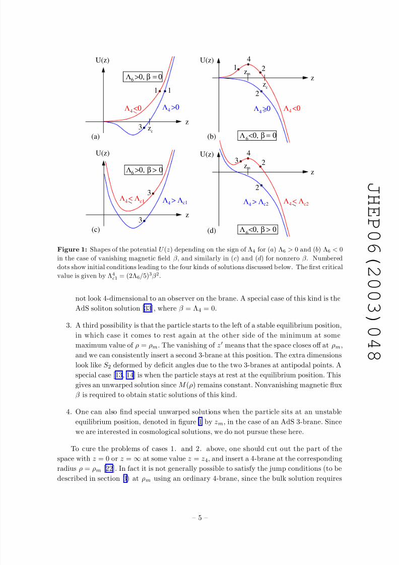
there is a magnetic flux. These are summarized in figure 1. The solutions can be visualized

by starting the particle at rest (z = 0) at position ρ = 0 with some initial value z0, and

letting it roll in the potential. The position ρ should be thought of as time in the mechanicsanalogy. The initial condition that z = 0 implies that M = 0 at ρ = 0, which must be the

case; there is no singular source term for M in the Einstein equations, and therefore M

must be continuous at the origin. Considering M evaluated along a straight line passing

through the origin, one sees that continuity of the slope requires that M in fact vanishes.

Using the mechanics analogy, a closed form solution for M (ρ) is implicitly provided by

integrating the equation of energy conservation, E = 12 z2 + U (z):

ρ =

zz0

dz

2(E − U (z))

. (2.10)

Once the particle starts rolling, there are four possible outcomes, which depend on theshape of the potential and the initial value z0.

1. In one kind of solution, the particle can reach z = 0 at some finite value of ρ. This

happens when β = 0, Λ6 > 0 and E > 0 (figure 1a), or when β = 0, Λ6 < 0, Λ4 < 0

and z < zm (figure 1b). Some curvature invariants diverge, so the extra dimensions

end at a singularity with the topology of S 1 in this case [23].

2. Another kind is where z → ∞ as ρ → ∞, as occurs if Λ6 < 0 and Λ4 ≥ 0, or if

Λ6 < 0, Λ4 < 0 and z > zm. Then gravity will not be localized, and the world does

– 4 –



J

HEP 0 6 ( 2 0

0 3 ) 0 4 8

zc

zc

3

3

34

4

Λ > Λ4 c1 _

4 c1Λ < Λ

z

U(z)

(c)

Λ >0, β > 06 z

Λ <0, β > 0

U(z)

zm

(d)

2

2

6

z

U(z)

_

(a)

3

1 1

Λ >0, β = 06

4Λ >04

z

Λ <0, β = 0

Λ <0_

U(z)

zm

(b)

1

2

2

Λ >04 4

6

Λ <0

Λ > Λ4 c2 _

4 c2Λ < Λ

Figure 1: Shapes of the potential U (z) depending on the sign of Λ4 for (a) Λ6 > 0 and (b) Λ6 < 0

in the case of vanishing magnetic field β , and similarly in (c) and (d) for nonzero β . Numbered

dots show initial conditions leading to the four kinds of solutions discussed below. The first critical

value is given by Λ4

c1= (2Λ6/5)3β 2.

not look 4-dimensional to an observer on the brane. A special case of this kind is theAdS soliton solution [33], where β = Λ4 = 0.

3. A third possibility is that the particle starts to the left of a stable equilibrium position,

in which case it comes to rest again at the other side of the minimum at some

maximum value of ρ = ρm. The vanishing of z means that the space closes off at ρm,

and we can consistently insert a second 3-brane at this position. The extra dimensions

look like S 2 deformed by deficit angles due to the two 3-branes at antipodal points. A

special case [13, 14] is when the particle stays at rest at the equilibrium position. This

gives an unwarped solution since M (ρ) remains constant. Nonvanishing magnetic flux

β is required to obtain static solutions of this kind.

4. One can also find special unwarped solutions when the particle sits at an unstable

equilibrium position, denoted in figure 1 by zm, in the case of an AdS 3-brane. Since

we are interested in cosmological solutions, we do not pursue these here.

To cure the problems of cases 1. and 2. above, one should cut out the part of the

space with z = 0 or z = ∞ at some value z = z4, and insert a 4-brane at the corresponding

radius ρ = ρm [22]. In fact it is not generally possible to satisfy the jump conditions (to be

described in section 3) at ρm using an ordinary 4-brane, since the bulk solution requires

– 5 –



J

HEP 0 6 ( 2 0

0 3 ) 0 4 8

that its stress-energy components T θθ differ from the other spatial components T ii. One

way of accomplishing this is to imagine that a pure tension 4-brane is accompanied by a

3-brane which is smeared around the compact extra dimension [34], or by Casimir energy

of a massless field confined to the 4-brane [17]. Alternatively, it is possible to find a special

value of ρm where the jump conditions on M and L can both be satisfied for a pure tension4-brane, as long as Λ4 is nonzero. By integrating the exact result (4.10) which we will

derive in section 4.3, this value is implicitly given by ρm0

M 2L dρ =L(0)

Λ4(2.11)

showing that ρm → ∞ as Λ4 → 0 for the warped solutions where M and L grow expo-

nentially. If one wants a solution which remains compact in the static limit, this is not

acceptable.

For completeness we mention one other kind of solution: we can start with z = 0

at ρ = 0, but in this case the position ρ = 0 should not be regarded as a single point,but rather the location of another 4-brane. A special case is when Λ6 < 0, Λ = E = 0;

then the warp factor takes the simple exponential form of the RS model. In fact this is

just the 5D RS solution augmented by one extra compact dimension, whose warp factor

is identical to that of the large dimensions. This model does not involve 3-branes, and is

mathematically quite similar to the 5D case which has been so well studied already. A

more thorough examination of the cosmology of these solutions in presented in appendix B,

and we comment upon its qualitative differences relative to the codimension two case in

the conclusions.

In the following subsections we present some specific analytic solutions illustrating the

cases mentioned above.

2.1 Type 1 solutions

A solution which is borderline between type 1 and type 3 can be found by choosing Λ 4, Λ6 >

0, E = 0. Starting from z = zc = (b/a)5/4, the critical value shown in figure 1a defined by

U (zc) = 0, the particle subsequently rolls toward z = 0. The solution is

M (ρ) = cos (kρ) ; L(ρ) = Rk sin(kρ) ; k =

Λ6

10= H , (2.12)

where we have used the freedom to rescale xµ to make M (0) = 1. Recall that H = Λ4/3

is the Hubble constant, so that Λ4 is determined by

Λ4 =3

10Λ6 . (2.13)

Interestingly, no curvature invariants diverge at the point ρm = π/2k where M = 0 and

the space should be terminated. In fact the Ricci scalar is constant, R = 3Λ6, and so are

the Ricci tensor squared Rαβ Rαβ = 3

2 Λ26, and Riemann tensor squared RαβγδRαβγδ = 3

5 Λ26.

The Weyl tensor vanishes. This is analogous to the behavior as y → ∞ in the 5D Randall-

Sundrum solution [35] with the line element ds2 = e−2k|y|(−dt2 + dx 2) + dy2; even though

– 6 –



J

HEP 0 6 ( 2 0

0 3 ) 0 4 8

the warp factor vanishes as y → ∞ in this model, there is no singularity. Although

M (ρm) = 0, yet z = 5/2M 3/2M vanishes at ρm, so in the mechanics analogy, the ball

rolls to the top of the hill and comes to rest again. Apparently the 4D part of the spacetime

disappears at ρm, leaving one with just 2D euclidean space in the ρ-θ plane.

In the case of vanishing Λ4 and positive Λ6, the following solution can be found [9]

M (ρ) = cos (kρ)2/5 ; L(ρ) = Rk sin(kρ)2/5 ; k =

5

8Λ6 . (2.14)

In this case however, in the mechanics analogy the particle does not come to rest at z = 0,

and there will be a curvature singularity at that point. It is therefore necessary to insert a

4-brane at ρ < ρs to cut off the space before reaching the point where it becomes singular.


It is interesting to consider solutions with Λ6 < 0 since this gives a warped geometry, where

the hierarchy problem can be solved on the 3-brane a la Randall-Sundrum. We find asolution of type 2 when β = E = 0 and Λ4, Λ6 < 0 by analytically continuing (2.12) in Λ4

and Λ6:

M (ρ) = cosh (kρ) ; L(ρ) = Rk sinh(kρ) ; k =

|Λ6|10

= iH . (2.15)

This follows the upper curve of figure 1b, starting at zc. The Hubble constant is imaginary

because the 4D metric is AdS space. In addition the E = 0 type 2 solution with Λ4 > 0

and Λ6 < 0 is

M (ρ) = sinh(kρ) ; L(ρ) = Rk cosh (kρ)

which follows the lower curve of figure 1b, starting at z = 0. However, this solution doesnot admit a 3-brane at ρ = 0 since L is nonvanishing at this point.

The only way to admit a 3-brane at ρ = 0 if Λ4 ≥ 0 is to take E < 0, so that the

initial condition z = 0 (equivalent to the boundary condition M = 0) can be satisfied.

The static solution with Λ4 = 0 (and β = 0) has been investigated in [34, 22]; this is the

AdS soliton truncated at large ρ by a 4-brane:

M (ρ) = cosh25 (kρ) ; L(ρ) =

2

5Rk

sinh(kρ)

cosh35 (kρ)

k =

−5

8Λ6 . (2.16)

Analytic expressions for M (ρ) in the AdS soliton type of solution no longer exist when

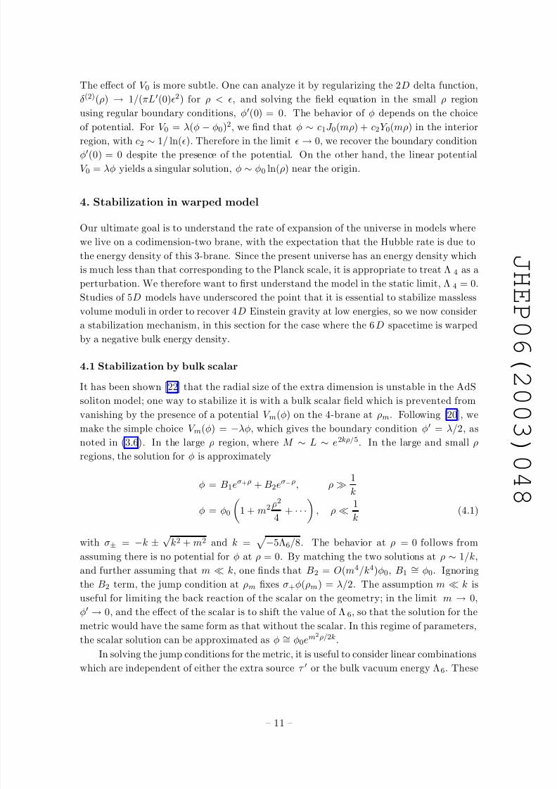
Λ4 > 0. However, we can obtain approximate analytic solutions by considering Λ 4 as aperturbation. The details are given in appendix A. The result is that the unperturbed

solution gets shifted according to

M (ρ) = [z0 cosh(k(ρ + δρ))]2/5 ; L(ρ) = RM (ρ) , (2.17)

where δρ(z) has the shape shown in figure 2, and z = z0 cosh(kρ). At sufficiently large

values of ρ, the shift δρ approaches a constant, so at leading order the only difference

between the perturbed and unperturbed solutions at large ρ is a shift in the radial size of

the extra dimension.

– 7 –



J

HEP 0 6 ( 2 0

0 3 ) 0 4 8

0.51

δρ

1 2 3 4 5 6 7 8 9z

Figure 2: δρ versus z, due to nonzero Λ4 in the AdS soliton solution.


The simplest example of a solution of type 3 is that in which the particle sits at a minimum

of U . In this case M is constant, so the solution is unwarped. If there is no magnetic field,

this occurs only in figure 1a, when Λ4 > 0. To specify the physical value of Λ4, we

should rescale M → 1 so that time and energy are normalized in the usual way (ds2 =

−dt2 + e2Htdx 2). Since Λ4 = 3H 2, which has dimensions of (mass)2, the relevant quantity

is Λ4/M 2 = Λ6/2; in other words the expansion rate is governed completely by Λ 6, which

is to be expected since it is the only source of stress energy.

Another example of unwarped solutions is the static case Λ 4 = 0 with nonvanishing

magnetic field. Just like above we noted that the physically relevant combination for the

expansion rate is Λ4/M 2, in this case β 2/M 8 is the meaningful combination for the square

of the magnetic field strength. Minimizing U (z) we find that β 2/M 8 = 2Λ6, in agreement

with references [13, 14]. Notice that Λ6 must be positive to achieve this fine tuning with

the magnetic flux.

In fact, the general relation between Λ4, Λ6 and β can be easily found in the same

way, demanding U (z0) = 0, when we realize that there is the freedom to set z0 → 1 by

rescaling xµ → xµ/z0. Thus

Λ4 =1

2 Λ6 −1

4 β 2 (2.18)

characterizes the physical expansion rate for an observer on the 3-brane when the bulk

parameters are not tuned to give a static solution. This is a significant result because it is

completely independent of the tension of such a 3-brane [13, 14].

Although M is trivial for the unwarped solutions, L is nontrivial:

L(ρ) = R sin(kρ) ; k2 =1

2Λ6 +

1

4β 2 (2.19)

as follows from solving the (µµ) Einstein equation (2.1), using (2.18) to eliminate Λ4.

More general solutions of type 3 cannot be found exactly, but an approximation is

possible for values of E which are sufficiently close to the bottom of the potential infigure 1a so that it can be treated like a harmonic oscillator. This gives

M (ρ) ∼= (z0 + cos(kρ))2/5 , (2.20)

where z0 is the position of the minimum of the potential, and k2 = U (z0). In general

k and are functions of Λ6, Λ4 and β . For example, in the case without magnetic flux,

z0 = (2Λ4/Λ6)5/4 and k2 = 12 Λ6. If one wants to rescale the warp factor to unity, the

physically meaningful place to do so is on the brane where the observer is supposed to be,

for example z0 + → 1.

– 8 –



J

HEP 0 6 ( 2 0

0 3 ) 0 4 8

Interestingly, in the more general solution (2.20), some dependence of the expansion

rate on the tensions τ 3, τ 3 of the two 3-branes appears. An application of the jump

conditions to be described in section 3.1 gives the following constraint:

τ 3 − 2πτ 3 − 2π =

z0 − z0 + 3/2

. (2.21)

This can be regarded as a fine tuning between the brane tensions required to obtain a given

value of the expansion rate determined by Λ4. There is a one-parameter family of brane

tensions which preserve the necessary relationship, showing that the expansion rate is not

uniquely determined by the brane tensions. However the degeneracy of solutions along

this curve in the τ 3-τ 3 plane does not constitute a solution to the cosmological constant

problem, and in this respect we disagree with the interpretation of [5]. In that reference,

it was assumed that a deficit angle could appear spontaneously at the position of one of

the branes, without having to specify any brane tension in the input to the construction

of the model, namely the stress-energy tensor. Our point of view is that the 3-brane isnot created by the geometry, but rather any singularity in the 2 D curvature is due to the

presence of a 3-brane with nonvanishing tension. (Another difference between our work

and that of [5] is that we do not assume the deficit angle, hence brane tension, to be zero

at ρ = 0. This enlarges the class of solutions we are considering.)

3. Brane tensions and jump conditions

In the previous section we generalized the analysis of [4] to include extra sources of stress

energy and to consider all possible signs of these various sources. A further new ingredi-

ent which [4] did not consider is the presence of branes which bound the bulk solutionsgiven above. In each case we wish to allow for a 3-brane at the origin of the two extra

dimensions, ρ = 0, which could provide support for the standard model and our observable

4D spacetime. (A special case is a 3-brane with vanishing tension, which is the same as

no brane as far as Einstein’s equations are concerned.) The space will either terminate

with another 3-brane or a 4-brane at some maximum value ρm, or it may be noncompact,

according to the possiblities mentioned in section 2, although the latter situation is not

compatible with recovering 4D gravity at large distances.

3.1 Jump condition at ρ = 0

In all cases, the constant of integration R in (2.8) is related to the tension τ 3 of the 3-brane at ρ = 0. If τ 3 is nonzero, there is a conical defect with deficit angle δ given by

δ = κ26τ 3, where κ2

6 = 8πG6, in terms of the 6D Newton’s constant. We can compute the

ratio of the circumference and the radius of an infinitesimal circle around the origin as

lim→0 2πL()/ = 2πL(0). Therefore, continuing to work in units where κ6 = 1, we have

τ 3 = 2π(1 − L(0)) . (3.1)

If the space is terminated by another 3-brane at ρm with tension τ 3, the relation becomes

τ 3 = 2π(1 + L(ρm)) . (3.2)

– 9 –



J

HEP 0 6 ( 2 0

0 3 ) 0 4 8

3.2 Metric jump conditions at ρ = ρm

On the other hand, if there is a 4-brane at ρm, it may need to be accompanied by some

additional form of stress energy in order to cut the bulk solution at this particular location,

because there are separate jump conditions for the θθ and µµ components of the Einsteinequations. Therefore one generally needs two tunable parameters to satisfy both conditions.

These conditions can be inferred from looking at the terms in the Einstein equations which

have second derivatives or delta functions:

µµ :M

M +

1

3

L

L+

M L

M L+

M 2

M 2= −1

3T 0

0 δ(ρ − ρm) + · · ·

θθ : 2M 2

M 2+

4M

3M = −1

3T θθ δ(ρ − ρm) + · · · . (3.3)

We will impose Z 2 symmetry at the 4-brane so that the discontinuity in M is −2M .

Integrating in the vicinity of the delta functions, we find

T 00 = 6

M

M + 2

L

L; T θθ = 8

M

M , (3.4)

where the functions are all evaluated at ρm. If the stress energy tensor was given by a

brane with pure tension, we would have T 00 = T θθ . This does not occur in the static AdS

soliton solution (2.16), where M /M − L/L is always nonzero, except as ρ → ∞. One

way to obtain a difference between T 00 and T θθ is to “smear” a 3-brane along the compact

dimension of the 4-brane [34]. Since the 3-brane has T θθ = 0, this procedure will give

an extra contribution only to the T µµ components. The shift in T 00 due to the smeared

3-brane tension τ 3 is given by T 00

−T θθ = τ 3/[2πL(ρm)]. This is not the only way to obtain

a deviation T 00 − T θθ ; for example the Casimir energy of a massless field confined to the

4-brane gives T 00 −T θθ ∼ L−5 [17]. In general, the energy density of the source τ can scale

like 1/Lα(ρm), where α determines its equation of state. Conservation of stress-energy

then dictates its contributions to the different components of the stress tensor [9, 22]:

T 00 = T 4 + V m(φ) +

τ

Lα(ρm)

T θθ = T 4 + V m(φ) + (1 − α)τ

Lα(ρm). (3.5)

The scalar field potential V m(φ) is explained in the next subsection.

3.3 Jump conditions for φ

In the absence of delta function sources for φ, regularity of the solutions requires that

φ(0) = φ(ρm) = 0. If potentials V 0(φ)δ(2)(ρ), V m(φ)δ(ρ − ρm) are included in the la-

grangian, φ may be nonzero at these points. The effect of V m is easily found by integrating

the φ equation of motion in the vicinity of ρm assuming Z 2 symmetry:

φ(ρm) = −1

2

dV mdφ

. (3.6)

– 10 –



J

HEP 0 6 ( 2 0

0 3 ) 0 4 8

The effect of V 0 is more subtle. One can analyze it by regularizing the 2D delta function,

δ(2)(ρ) → 1/(πL(0)2) for ρ < , and solving the field equation in the small ρ region

using regular boundary conditions, φ(0) = 0. The behavior of φ depends on the choice

of potential. For V 0 = λ(φ

−φ0)2, we find that φ

∼c1J 0(mρ) + c2Y 0(mρ) in the interior

region, with c2 ∼ 1/ ln(). Therefore in the limit → 0, we recover the boundary conditionφ(0) = 0 despite the presence of the potential. On the other hand, the linear potential

V 0 = λφ yields a singular solution, φ ∼ φ0 ln(ρ) near the origin.

4. Stabilization in warped model

Our ultimate goal is to understand the rate of expansion of the universe in models where

we live on a codimension-two brane, with the expectation that the Hubble rate is due to

the energy density of this 3-brane. Since the present universe has an energy density which

is much less than that corresponding to the Planck scale, it is appropriate to treat Λ 4 as a

perturbation. We therefore want to first understand the model in the static limit, Λ 4 = 0.

Studies of 5D models have underscored the point that it is essential to stabilize massless

volume moduli in order to recover 4D Einstein gravity at low energies, so we now consider

a stabilization mechanism, in this section for the case where the 6D spacetime is warped

by a negative bulk energy density.

4.1 Stabilization by bulk scalar

It has been shown [22] that the radial size of the extra dimension is unstable in the AdS

soliton model; one way to stabilize it is with a bulk scalar field which is prevented from

vanishing by the presence of a potential V m(φ) on the 4-brane at ρm. Following [20], wemake the simple choice V m(φ) = −λφ, which gives the boundary condition φ = λ/2, as

noted in (3.6). In the large ρ region, where M ∼ L ∼ e2kρ/5. In the large and small ρ

regions, the solution for φ is approximately

φ = B1eσ+ρ + B2eσ−ρ, ρ 1

k

φ = φ0

1 + m2 ρ2

4+ · · ·

, ρ 1

k(4.1)

with σ± =

−k

±

√k2 + m2 and k = −5Λ6/8. The behavior at ρ = 0 follows from

assuming there is no potential for φ at ρ = 0. By matching the two solutions at ρ ∼ 1/k,

and further assuming that m k, one finds that B2 = O(m4/k4)φ0, B1∼= φ0. Ignoring

the B2 term, the jump condition at ρm fixes σ+φ(ρm) = λ/2. The assumption m k is

useful for limiting the back reaction of the scalar on the geometry; in the limit m → 0,

φ → 0, and the effect of the scalar is to shift the value of Λ 6, so that the solution for the

metric would have the same form as that without the scalar. In this regime of parameters,

the scalar solution can be approximated as φ ∼= φ0em2ρ/2k.

In solving the jump conditions for the metric, it is useful to consider linear combinations

which are independent of either the extra source τ or the bulk vacuum energy Λ6. These

– 11 –



J

HEP 0 6 ( 2 0

0 3 ) 0 4 8

linear combinations are

− λφ + T 4 =

6 +

2

α

M

M +

2 − 2

α

L

L≡

6 +2

α

µ +

2 − 2

α

(4.2)

ατ

2Lα =L

L −M

M ≡ − µ , (4.3)

where all quantities are to be evaluated at ρ = ρm. The right hand side depends only on

ratios where the overall normalization of the metric elements cancel out, whereas the left

hand side depends on L itself. Using L = RM , L = RM , L(0) = 1 − τ 3/2π and (2.2),

(2.16) to evaluate M (0) = 2k2/5, we can show that the constant R equals (5/2k2)(1− τ 32π ).

(Recall that we have rescaled the 4D coordinates xµ so that M (0) = 1). Then L can be

expressed as

L =5

2k−2

1 − τ 32π

M ∼= k−1

1 − τ 32π

M , (4.4)

where the latter approximation holds for ρ

1/k. Eqs. (4.2) and (4.3) determine ρm, the

position of the 4-brane, and they give a constraint on some function of T 4, τ 3 and τ . The

latter is the fine-tuning which must be done in order to obtain a static solution. We will

carry this out explicitly below.

4.2 Back reaction of scalar (or magnetic flux) on metric

To solve the jump conditions (4.2) and (4.3), we need to know how the scalar perturbs the

metric. Although we will consider stabilization by the scalar and not the flux, for generality

we indicate how the same analysis can be carried out for stabilization by flux. Similarly,

we can also compute the perturbation away from the static solution by keeping the effect

of the 4D cosmological constant, even though our immediate goal is to examine the static

solution.

Let δµ be the perturbation to M /M in eq. (2.2), which when linearized takes the form

δµ + 5µ δµ =1

8

4

Λ4

M 2− φ2 − m2φ2 +

n2φ2

L2+

β 2

M 8

. (4.5)

The part of δµ in the absence of flux, winding, or cosmological expansion, due only to the

stabilization mechanism, is

δµφ ≡ δ

M

M

= −1

8M −5

ρ0

dρ (φ2 + m2φ2)M 5

∼= − m2φ20

64 cosh2(kρ)

e2(k+σ+)ρ − 1

k + σ++ 2

e2σ+ρ − 1σ+

+e2(−k+σ+)ρ − 1

−k + σ+

. (4.6)

It can be shown that in the m k limit in which we are interested, it is always true that

φ2 m2φ2, so we dropped the derivative term to obtain (4.11). Similarly the decaying

exponential part of φ gives only subdominant contributions in m2, so we approximated

φ = φ0eσ+ρ. Now eq. (4.6) can be integrated again to find the deviation in M itself,

δM φM

=

ρ0

dρδµφ∼= − λ2

16m2kρm (at ρ = ρm) , (4.7)

– 12 –



J

HEP 0 6 ( 2 0

0 3 ) 0 4 8

where in the last approximation we have kept only the leading behavior in m2. The

last result shows that λ2kρm/m2 must be kept small in order for the perturbation to be

under control. Notice that we have used our freedom to impose the boundary condition

δM φ(0) = 0 to preserve the normalization M (0) = 1.

To compute the analogous shift δφ in L/L, we perturb eq. (2.3). In fact it will beconvenient to compute δφ − δµφ,

δφ − δµφ = −

4 +

µ

δµφ +

1

8µ(φ2 − m2φ2) . (4.8)

Using /µ = (5 coth2(kρ) − 3)/2 and µ = (2k/5) tanh(kρ) for the unperturbed quantities,

we can explicitly integrate (4.8) from 0 to ρ. The result is

δLφ

L− δM φ

M =

5

16

λ2

m2 e−2σ+ρ − 1

2 + m2/k2+ O

e−2kρ

. (4.9)

This result will be essential for finding the size of the radial extra dimension ρm from the

stabilization mechanism.

4.3 Solution of jump conditions

We are now ready to solve for ρm and the fine-tuning between stress-energy components

which leads to the static solution. Toward this end, it is useful to rewrite the difference

between eqs. (2.2) and (2.1) in the form

M 4L(µ

−) = M 4L

Λ4

M 2

+n2φ2

L2

+β 2

M 8 . (4.10)

If we are only interested in stabilization by the Goldberger-Wise mechanism, and the static

solution, then the right hand side of (4.10) vanishes, leading to

− µ =c

M 4L=

L(0)

M 4L, (4.11)

where we evaluated the equation at ρ = 0 to evaluate the constant of integration c. Com-

bining (4.11) with the jump condition (4.3), we find the equation which determines the ρm,

namely 2L(0)/ατ = M 4L1−α. The only hope for obtaining the desired large hierarchy

ρm

1/k is in the case where α = 5. Otherwise we obtain e2(1−α/5)kρm

∼L(0)/τ , which

gives a large hierarchy only by tuning τ to be unnaturally small in units of the 6D gravity

scale. On the other hand, in the case α = 5, we must rely on the small correction (4.9) to

find the leading ρ dependence in the jump condition,

y ≡ 2

5τ

1 − τ 3

2π

=

M

L

4= 1 − 4

δLφ

L− δM φ

M

+ O

e−2kρm

. (4.12)

The result for ρm is

ρm = − k

m2ln

4m2

5λ2(1 − y) +

1

2

. (4.13)

– 13 –



J

HEP 0 6 ( 2 0

0 3 ) 0 4 8

This solution only exists if τ lies in the range

2

1 − τ 32π

51 + 5λ2

8m2< τ <

2

1 − τ 32π

51 − 5λ2

8m2(4.14)

This range could have had a large upper limit if 5λ2/8m2 1. However we found in (4.7)

that in fact we must have λ2/m2 < 1/(kρm) in order for perturbation theory to not break

down. So we see that there is still a fine tuning on τ for this model to give a large hierarchy.

It is qualitatively different from the kind of tuning that would occur in models with α < 5;

for these one would need to make the magnitude of τ exponentially smaller than its natural

scale in terms of the 6D gravity scale. For α = 5, the magnitude of τ can be natural, but

it must be very close to a specific value. One virtue of the scalar field is that it reduces

the amount of tuning which is necessary. A similar tuning was present in the absence of

the scalar field: (4.12) shows that y must be exponentially close to 1 if φ is absent, and if

we insist on getting a large hierarchy. Once φ is introduced, y must still be close to 1, but

no longer with exponential precision.

We could simply give up the tuning of τ and live with a model which does not try to

solve the hierarchy problem. But since the main purpose of this paper is to explore the

strange cosmological properties of this kind of model, questions of naturalness of the choice

of parameters are secondary. It is convenient to adhere to the strongly warped case, since

the hierarchy simplifies the algebraic analysis. We have seen that even in the completely

unwarped case, similar behavior is revealed, concerning the unusual dependence of the

Hubble rate on the brane tension is concerned.

The remaining jump condition (4.2) is the fine tuning that must be imposed to make

the effective 4D cosmological contant Λ4 vanish:

T 4 − λ2k2

2m2− 16

5k = 5τ e−2kρm

1 +

5λ2

16m2kρm

(4.15)

underscoring the fact that ultimately one needs an additional mechanism to fully solve the

cosmological constant problem in these models. Our purpose here is not to address the

problem of the 4-D cosmological constant, but rather the possible cosmological solutions

of codimension-2 braneworlds.

4.4 Stabilization by magnetic flux?

We can attempt to stabilize the warped solution using magnetic flux; however since the

effects of the flux are highly suppressed at large ρ because of the large exponential factor1/M 8, it is not clear that it actually can stabilize the highly warped solution. Following

the same steps as for the scalar field, we find

δµβ =β 2

8cosh2(kρ)

ρ0

dρM −3 ∼= β 2

8k cosh2(kρ)

c0 + c1e−6kρ/5 + c2e−c3kρ

,

where the approximate fit has c0 = 1.38, c1 = −1.91, c2 = −c0 − c1, c3 = −(1 + 65 c1)/c2

and in the large ρ limit

δLβ

L− δM β

M ∼= 5β 2

16k2

d0 + d1e−2kρ

,

– 14 –



J

HEP 0 6 ( 2 0

0 3 ) 0 4 8

where d0 = −0.66, d1 = 5.5. The resulting equation for ρm has the same form as (4.12),

except now the term δLβ /L− δM β /M depends on ρm only through e−2kρm, which is of the

same order as terms we ignored in (4.12). As explained there, this kind of dependence does

not allow for a large hierarchy unless τ is tuned with exponential precision to a special

value. This is exaclty the same situation as in the model with no stabilization, leading oneto suspect that magnetic flux does not actually stabilize this model, unless the warping is

weak (which would be the case if Λ6 > 0).

5. Friedmann equation in warped model

We now come to the main point of the paper, in the context of the AdS-type models: the

rate of expansion in the models we have described depends on the energy density (tension)

of the standard model 3-brane in a strange way, relative to our expectations from 4D

general relativity. Such an outcome would be less surprising if the low energy limit of the

model was a scalar-tensor theory of gravity, in which the coupling of the extra massless

scalar to the brane tension could explain the exotic effect. However we will note that the

conclusion is valid even when moduli have been stabilized. We now demonstrate this in

the warped case of the expanding AdS soliton model, (2.17), supplemented by a scalar field

which stabilizes the radion by the Goldberger-Wise mechanism [36, 17, 20, 22].

The main work has already been done in the previous section; there we found the back

reaction to the metric by treating the scalar field as a perturbation. In the same way we

can find the perturbation to the static solution due to a small rate of expansion by treating

the Λ4/M 2 term to first order. We have a double expansion, in Λ 4 and in φ2. We will work

to first order in either quantity, but not including the mixed terms of order Λ4φ2.

The perturbation δµΛ analogous to (4.6) is

δµΛ =1

2M −5

ρ0

dρΛ4

M 2M 5 (5.1)

∼= 5Λ4

12 · 26/5kcosh−2(kρ)

e6kρ/5 − 1 − a(e−kbρ − 1)

, (5.2)

where a = (26/5 − 1)2, b = (6/5)(26/5 − 1)−1. The integral cannot be done analytically, but

the appproximation (5.2) is chosen to give the correct large ρ behavior, and it matches the

exact value and its first derivative at ρ = 0; it is accurate to 0.6% everywhere, as shown in

figure 3.The shift in δ is given by

δΛ − δµΛ = −

4 +

µ

δµΛ +

Λ4

2µM 2. (5.3)

By numerical evaluation and empirically fitting, we find that the following expression is a

very good approximation to the integral of (5.3):

δLΛ

L− δM Λ

M ∼= 5

4

Λ4

k2

−1 + cosh−

45 (kρ)

. (5.4)

– 15 –



J

HEP 0 6 ( 2 0

0 3 ) 0 4 8

Figure 3: Ratio of the exact value of the integral in (4.11) to the approximation (5.2) as a function

of kρ.

Figure 4: Numerical integration of (5.3) versus kρ, and the approximation (5.4).

This captures with great accuracy asymptotic approach of the solution to its large ρ limit,

as well as having the correct small ρ behavior. The comparison between the exact result

and the approximation is shown in figure 4.

The new contribution to the jump condition determining the combination − µ from

(4.10) gives

− µ =1

M 4L

L(0) − ρ

0dρ

Λ4

M 2M 4L

=L(0)

M 4L

1 − 5Λ4

6k2(M 3 − 1)

, (5.5)

where we used (4.4) to perform the integral exactly. This modifies (4.12) by giving a new

term proportional to Λ4:

y ≡ 2

5τ

1 − τ 3

2π

∼= 1 +5λ2

16

e−2σ+ρ − 1

2

+

5Λ4

6k2M 3 , (5.6)

where we have ignored all exponentially small corrections.

Let us now recall what is the origin of the expansion of the universe according to our

assumptions. We are interested in starting from a static configuration, and then perturbing

it by adding some energy density on the 3-brane. Of course it is possible that the expansion

– 16 –



J

HEP 0 6 ( 2 0

0 3 ) 0 4 8

of our own universe could be due to a small mismatch of bulk energy densities which are

distributed in the extra dimensions. But our specific interest in this paper is to see how

the energy density on the 3-brane affects the Hubble expansion. Therefore we will make

the assumption that the quantity whose value is relaxed relative to the static fine-tuned

situation is τ 3; hence in our perturbation series δτ 3 and Λ4 are of the same order. Whencomparing (5.6) to the corresponding relation (4.12) for the static solution, there is one

other quantity which must in general vary: the position of the 4-brane ρm will deviate by

some amount δρm. However, all terms containing δρm are or order Λ4φ2 or Λ24 and so can

be neglected. Therefore the difference between (5.6) and (4.12) gives

Λ4 = −3k2

5π

δτ 31 − τ 3

2π

cosh−6/5(kρm) (5.7)

where we used the constraint (4.14) to eliminate τ . This is the result we have been seeking,

which shows an unexpected relation between Λ4 and δτ 3: a decrease in the energy densityon the 3-brane leads to cosmological expansion in this model.

It is straightforward to give the more general version of eq. (5.7), for arbitrary values

of α, and without assuming that we are perturbing around a static solution. We find that

Λ4 =6k2

5(M 3 − 1)

1 − αM 4L1−ατ

2

1 − τ 32π

, (5.8)

where M and L are to be evaluated at ρm. This shows that the surprising dependence

on τ 3 is not due to fine tuning of parameters. The Hubble rate is a decreasing function

of τ 3 quite generally in this model. By choosing τ 3 so as to make Λ4 = 0, and perturbingτ 3 → τ 3 + δτ 3, one recovers eq. (5.7).

When we perturb the other jump condition (4.2), we obtain an equation for the shift

in ρm, µ +

1

5( − µ)

δρm + δµΛ +

1

5(δΛ − δµΛ) = 0 (5.9)

which gives

δρm =−5Λ4

32k3

e2kρm

cosh45 (kρm)

=3

20π

δτ 3kτ

. (5.10)

6. Stability of unwarped model

As already pointed out in eq. (2.19), it is possible to find unwarped solutions [13, 14]

where the bulk is a two-sphere stabilized by magnetic flux. In these models the expansion

rate is insensitive to the three brane tension. To be sure that this unusual behavior is not

related to the presence of unstabilized moduli, in this section we perform a more complete

analysis of the stability of the model than was done in ref. [30]. In the following we will

set M = 1. We will consider in detail the static case and then give the main results of the

analysis in the presence of the expansion.

– 17 –



J

HEP 0 6 ( 2 0

0 3 ) 0 4 8

In the static case Λ4 = 0 and, from eqs. (2.1)–(2.2) we have

2 + = −β 2 , Λ6 =β 2

2. (6.1)

The fluctuations of this model may be classified according to four-dimensional Lorentz

transformations. On top of the usual transverse and traceless tensor (i.e. ∂ µhµν = hµ

µ = 0)

corresponding to five degrees of freedom there are three divergenceless vector modes (cor-

responding to nine degrees of freedom) and seven scalar modes. Overall, the perturbed

six-dimensional metric has 21 degrees of freedom. These 21 fluctuations of different spin

transform under coordinate transformations parametrized by the infinitesimal shift A ≡(µ, ρ, θ). The infinitesimal shift µ along the four-dimensional spacetime can be decom-

posed, in turn, as the derivative of a scalar and a divergenceless vector, i.e. µ = ∂ µ + ζ µ.

It is now easy to see that there are 3 scalar gauge functions ( ρ, θ and ) and one vector

gauge-function. Of the seven scalar degrees of freedom, three of them can be gauged awayby using the scalar gauge functions. Alternatively, the seven gauge-dependent scalars can

be rearranged into four gauge-invariant scalar fluctuations. In the context of the study of

six-dimensional abelian vortices [40, 41] it was shown that a convenient gauge choice brings

the line element in the form

ds2 = (1 − 2ψ)ηµν dxµdxν + (1 + 2ξ)dρ2 + L(ρ)2(1 − 12ϕ)dθ2 + 2πL(ρ)dρdθ (6.2)

where ηµν is the Minkowski metric. Since all the scalar gauge functions are completely fixed,

no spurious gauge modes will appear. Furthermore, it can be shown that the scalar fluc-

tuations appearing in (6.2) obey the same evolution equations of the four gauge-invariantfluctuations which have been defined, in general terms, in [41].

The four scalar fluctuations of the geometry are coupled, through the perturbed Ein-

stein equations

δRAB = δτ AB , τ AB = T AB − 1

4T C C GAB , (6.3)

to the scalar fluctuations of the sources whose evolution can be obtained by perturbing to

first order

∂ A

|G|F AB

= 0 . (6.4)

The two relevant fluctuations of the source are the fluctuations of the ρ and θ componentsof the vector potential. These fluctuations will be donoted as Aρ and Aθ. The divergence-

full part of the four-dimensional vector potential is also a scalar but it can be gauged away

by using the U(1) gauge symmetry.

Now that the gauge is fully fixed, we are ready to find the spectrum of fluctuations

for the class of unwarped models defined by (6.1). In connection with the automatic

adjustment of the solutions to cancel out any dependence on the tension of the 3-branes,

we are specifically interested in the radial modes and, therefore, the possible dependence

of the perturbed quantities upon the coordinate θ will be ignored. Using (6.2) the various

– 18 –



J

HEP 0 6 ( 2 0

0 3 ) 0 4 8

components of eq. (6.3) are

µ = ν : ξ = ϕ + 2ψ , (6.5)

µ = ν : ψ + ψ +ψ =

−β

2L

Aθ +

β 2

2

(ξ

−ϕ) , (6.6)

ρρ : ϕ + 4ψ + (2ϕ + ξ) − 3

2β 2ϕ − Λ6ξ −ξ =

3

2

β

LA

θ , (6.7)

θθ : ϕ + (2ϕ + ξ + 4ψ) − 3

2β 2ϕ +ϕ + 2

2 + +

3

4β 2

ξ =3

2

β

LA

θ , (6.8)

µρ : ϕ + (ϕ + ξ) + 3ψ =β

LAθ , (6.9)

µθ : π + 2π = − β

LAρ , (6.10)

θρ : π = 0 . (6.11)

where denotes the four-dimensional d’alembertian, −∂ 2

t +∂ 2

x. Eqs. (6.5)–(6.11) should besupplemented by the evolution equations describing the fluctuations of the sources which

can be obtained by perturbing eq. (6.4) to first order:

Aθ − A

θ + βL(4ψ + ξ − ϕ) +Aθ = 0 , (6.12)

Aρ = 0 , Aρ = 0 . (6.13)

Notice that π and Aρ are decoupled from the other equations. The resulting system of

coupled equations (6.11) and (6.13) implies that both π and Aρ are massless excitations.

Furthermore, since Aρ is constant, eq. (6.10) can be easily solved with the result that

π(ρ) =cπL2 − βAρ

dρL(ρ) . (6.14)

However this mode is not normalizable, hence it is unphysical. In the action perturbed to

second order the kinetic term for π appears multiplied by only one factor of L. Thus the

kinetic term for π diverges as ρ → 0, in agreement with the findings of [41].

The remaining longitudinal degrees of freedom (i.e. ϕ, ψ, ξ and Aθ) satisfy a cou-

pled set of linear differential equations whose eigenvalues determine the stability of the

solution (6.1). The boundary conditions to be imposed at the origin are [22]:

ϕ(0) + ξ(0) = 0 , ψ(0) = 0 , Aθ(0) = 0 . (6.15)

If we now consider eq. (6.5) we see that, for ρ → 0, eqs. (6.15) imply

φ(0) + ψ(0) = 0 . (6.16)

It is convenient to define two new variables:

ψ =X − Y

2, ξ =

X + Y

2. (6.17)

With these variables we will have that the linear combination 3 × (µ, ν ) + (θ, θ) leads to

X + 3X + (− β 2)X = β 2Y (6.18)

– 19 –



J

HEP 0 6 ( 2 0

0 3 ) 0 4 8

while the difference of the (ρ, ρ) and (θ, θ) components of the perturbed Einstein equations

(6.7) and (6.8) gives

X − Y − (X − Y ) = Y (6.19)

and eq. (6.9) determines the gauge field

Aθ =L

β (X + 2Y ) . (6.20)

In terms of X and Y the boundary conditions (6.15) are now X (0) = Y (0) and Y (0) = 0.

It is easy to verify that one solution to the coupled equations (6.18, 6.19) matches the

results of ref. [30], with X = constant, Y = 0, and mass eigenvalue

m2r = β 2 (6.21)

which is the radion mass squared of this model. Although the analysis of [30] was in

a 4D effective theory, their result is exact since the solution has no dependence on the

extra dimension. The constancy of the wave function shows that this must indeed be the

ground state of the system (6.18) and (6.19), since nonconstant solutions should have higher

energy and correspond to Kaluza-Klein excitations of the ground state. Nevertheless to be

thorough we have conducted a numerical search for other eigenstates using the shooting

method, and verified that (6.21) is indeed the ground state solution.

The same analysis can be done in the case where the background solution has de Sitter

expansion, as in eq. (2.19), rather than being static. The system (6.18) and (6.19) becomes

X + 3X + X

− β 2 +

33

4H 2

=

β 2 + 12H 2

Y

X

−Y

−(X

−Y ) = +

9

4

H 2 . (6.22)

The form of the bulk solution is the same as when H = 0, but the mass eigenvalue

generalizes to

m2r = β 2 − 33

4H 2 , (6.23)

showing that a sufficiently large rate of expansion destabilizes the compactification.

Let us now discuss the vector modes, which must be considered in a fully consistent

decomposition of the metric and source fluctuations 6D. It was recently shown in [14] that a

massless graviphoton field is present in the low-energy spectrum. In the following we restrict

ourselves to the spectrum of the vector excitations with only radial dependence. The θ

dependence of the perturbed quantities, considered in [40], would presumably correspond

to KK excitations of the lowest modes which we seek here.

Denoting by V µ and Z µ the divergenceless graviphoton fields appearing, respectively,

in the (µ, ρ) and (µ, θ) components of the perturbed metric, the equations for the coupled

system of vector fluctuations reads:

µ = ν : V µ + V µ = 0 , (6.24)

µρ : V µ = 0 , (6.25)

µθ : Z µ + Z µ + Z µ +Z µ + 2βAµ = 0 , (6.26)

µ : Aµ + A

µ +Aµ − β [Z µ + Z µ] = 0 , (6.27)

– 20 –



J

HEP 0 6 ( 2 0

0 3 ) 0 4 8

where Aµ is the divergenceless fluctuation of the vector potential and eq. (6.27) follows

from the perturbed component of the evolution equation of the gauge field.

From eq. (6.25) it follows that V µ is always massless in perturbation theory, as was

argued in [14]. This conclusion, valid for radial excitations, follows from the cancellation

of the contribution of Λ6 and the magnetic flux in the perturbed equations. Howevereq. (6.24) implies that V µ ∼ L−1. Like the π mode in (6.14) this mode is not normalizable

and therefore unphysical.

To analyze the coupled system of excitations for Z µ and Aµ notice that if the mode is

massless, then eq. (6.27) can be integrated once to find that Aµ = βZ µ. This allows us to

rewrite the equation for Z µ in a decoupled form:

Z µ + Z µ + Z µ + 2β 2Z µ = 0 . (6.28)

It is already known that in the case of the six-dimensional abelian vortex there exists a

normalizable vector zero mode [40, 41] (see also [42]). In our case, recalling (6.1), the zeromode takes the form

Aµ ∼ β

ρLdρ , Z µ ∼ L (6.29)

which is the ground state solution of eqs. (6.26) and (6.27). This mode is normalizable

since the canonical fields related to Aµ and Z µ are simply the original ones multiplied by√L. The localization of the gauge mode related to Aµ was recently invoked [40]–[42] as

a mechanism in order to localize gauge fields in the presence of thick abelian strings in

six-dimensions.

The masslessness of the graviphoton mode is not a concern, as would be a massless

scalar mode, due to the fact that the graviphoton couples only to T µθ, which vanishes on

the 3-brane. Since the graviphoton does not couple to standard model matter, it is not

phenomenologically constrained like a Brans-Dicke scalar. Moreover it does not seem a

likely candidate for explaining the tuning of the bulk geometry in response to a 3-brane

tension, since this is a deformation which looks like a purely scalar mode.

7. Discussion and conclusions

We have made a comprehensive review of 6D cosmologies which contain at least one 3-

brane where the standard model could presumably be localized. Emphasis was given to

several solutions in which the rate of expansion of the universe is either insensitive to the

tension of a 3-brane, eqs. (2.13) and (2.18), or else depends on τ 3 in a way which is at

odds with 4D general relativity eq. (5.7). This is despite the fact that we are considering

values of τ 3 which are well below the scale of compactification and the mass scale of

moduli which could account for a departure from conventional gravity. If the theories under

consideration contained a massless radion, for example, one would not be so surprised to see

such behavior. However both of the models we have focused on do have stabilized moduli.

The AdS soliton model has only a single radion among the fluctuations with azimuthal

symmetry. It is massless for α = 5 and has an exponentially small negative (mass)2 for

α < 5 in the absence of stabilization, but with the Goldberger-Wise mechanism it acquires

– 21 –



J

HEP 0 6 ( 2 0

0 3 ) 0 4 8

a positive (mass)2 of order m4k−2φ2(ρm)e−2kρm/5 ∼ λ2e−2kρm/5 [22]. For realistic values of

the hierarchy, this gives a radion mass of order MeV, which is safe because the couplings

of the radion to the 3-brane are suppressed by the 4D Planck scale. And in the previous

section we have confirmed the stability of the unwarped “football-shaped” model by doing

an exhaustive study of its perturbation spectrum.The tensions of 3-branes in two 6D theories fail to contribute to the Hubble rate in

the expected way at low energies, despite the fact that these theories have no additional

massless scalars that might explain a deviation from 4D general relativity. Instead, the

explanation of this apparent failure of decoupling lies in the special way in which a 2D

manifold’s internal geometry responds to the tension of a codimension two brane. This can

be seen from a direct dimensional reduction of the 6D theory to four dimensions [9].

Consider the metric (1.1) with a fluctuating 4D metric, g4,µν (xµ). When we integrate

the 6D Einstein-Hilbert action over the coordinates yi of the internal space, we obtain

L4,eff = 12κ2

6

|g4| d2y √g2M 2R4 − V 4,eff (7.1)

V 4,eff =

d2y M 4

√

g2

− 1

2κ26

R2 + Λ6 +1

4F 2 + · · ·

+i

τ 3,iδ(2)(y − yi)

, (7.2)

where Rn is the n-dimensional curvature constructed from gn,µν ; τ 3,i is the tension of the

ith 3-brane, and . . . denotes contributions from other sources such as the bulk scalar field

or a 4-brane. In the unwarped solution, where τ 3,1 = τ 3,2 ≡ τ 3, there are two cancellations

which make R4 independent of τ 3. First, the curvature R2 has singular contributions that

exactly cancel the delta function terms explictly involving the tensions. One can see the

crucial difference between codimension one and two branes by examining their respectivecontributions to R2 [34]:

R2

κ26

= 2τ 3 δ(2)(y) +1

2T 4 δ(1)(y − y4) + nonsingular terms . (7.3)

The coefficient of the 2D delta function is such as to cancel the similar contribution to

the action from the 3-brane’s stress-energy, whereas this cancellation is not exact for the

4-brane. The second cancellation of the dependence on the 3-brane tension is this: τ 3enters implicitly through the volume of the extra dimension,

g2(0) = L(0) = 1 − τ 3/2π

which multiplies the entire nonsingular part of the action, including the coefficient of R4

in (7.1), which gives the 4D Planck mass:

M 2 p =1

κ26

d 2y

√g2 M 2(y) . (7.4)

These two factors of L(0) cancel out of the Friedmann equation, H 2 = V 4,eff /3M 2 p , so that

the Hubble rate is determined completely by bulk quantities, independent of the brane

tension. Notice that one reason we can make this argument so simply in the unwarped

case is the fact that the bulk solution changes only through a rescaling of L as a result of

changing the brane tension.

– 22 –



J

HEP 0 6 ( 2 0

0 3 ) 0 4 8

When we try to make a similar argument to deduce the form of the Friedmann equation

in the warped solution, it is not straightforward, because M and L do change from their

static forms when the brane tension is changed, which induces a nonzero value of Λ 4. It is

still true that the delta function term τ 3δ(2)(y) is cancelled by a singular term of exactly

the same magnitude in √g2R2. But now there are additional terms of order Λ4 from theperturbation to the bulk part of the solution. These did not appear in the unwarped case.

The essential difference between the two models is that the jump conditions at the 4-brane

bring in a new source of dependence on L, hence the 3-brane tension, which does not exist

in the type 1 solution or in the unwarped type 3 solution. These observations were also

made in [9].

The hope would be to solve the cosmological constant problem by using bulk super-

symmetry to ensure Λ4 = 0, in a model where Λ4 is independent of the 3-brane tension.

Then Λ4 will be insensitive to all quantum corrections to the vacuum energy which arise

if the standard model is confined to the 3-brane. However to describe realistic cosmology,

one needs to depart from pure de Sitter space and look for Friedmann-Robertson-Walker

solutions. In fact, it is not obvious that solutions to the 6D Einstein equations exist when

cosmological matter and radiation are added to the brane. Let us suppose the line element

has the rather general form

ds2 = −N 2dt2 + M 2dx2 + B2dρ2 + L2dθ2 , (7.5)

where all the metric functions can depend on t as well as ρ, and consider the terms in the

Einstein equations which can have delta function singularities:

00 : 3

M M

+ M LM L

+ L

L∼ B2δ(2)(ρ) (7.6)

ii : 2

M

M +

M L

M L

+

N

N +

N L

N L

+

L

L∼ pB2δ(2)(ρ) (7.7)

θθ : 3

M

M +

M L

M L

+

N

N +

N L

N L

∼ 0 . (7.8)

In all the solutions we have considered, the energy density of the brane is given by ε =

− p = τ 3, and M = N = 0 at ρ = 0, so that there is no singular part in M or N .

To obtain ε = − p, it is necessary to have singular behavior not only in L/L, but also in

the other terms. However L

/L gives a 2D delta function δ(2)

(ρ) ∼ δ(ρ)/ρ by virtue of Lvanishing like ρ. We can only get this kind of behavior from M /M if M also vanishes,

which is not physically sensible since the standard model requires a nonvanishing metric.

The only way we see to admit a general equation of state is to give the 3-brane a finite

radius ρ0. A solution to the equation M + M /r = −εMδ(2)(ρ) can be found if δ(2)(ρ) is

a regularized delta function:

M (ρ) =

J 0(aρ), ρ < ρ0

J 0(aρ0) + aρ0J 1(aρ0) lnρ0

ρ, ρ > ρ0 ,

(7.9)

– 23 –



J

HEP 0 6 ( 2 0

0 3 ) 0 4 8

where a =

ε/(πρ20). For branes of codimension one, the interesting corrections to the

Hubble rate come from terms like (M /M )2, which are nonsingular and have an unam-

biguous value proportional to ε2. For the regularized codimension two brane, (M /M )2 ∼(ερ/ρ2

0)2 which goes like 1/ρ20 when averaged over the brane. Thus we expect to get results

which are sensitive to the internal structure of the brane, unlike the clean predictions thatcame from the codimension one case. Of course, unambiguous predictions could be made

in a specific theory, for example where the brane was a cosmic string defect coming from

an abelian Higgs model. Whether the interesting cosmological properties of codimension

two branes will survive after regularizing them requires further investigation.

Acknowledgments

We thank Daniel Chung, Rob Leigh and Dominik Schwarz for valuable discussions. J.C.,

J.D. and J.V. are supported in part by Canada’s National Sciences and Engineering Re-

search Council.

A. Perturbation to AdS soliton from small Λ4

Let us write E = E 0 + δE , where E 0 = az20 and δE = −bz

6/50 is an energy shift relative to

the static solution which allows us to keep the same starting value z0; then (E − U ) can

be written as

E − U (z) = a(z20 − z2) + b(z6/5 − z

6/50 ) (A.1)

and the b term can be consistently treated as a perturbation, even in the region ρ ∼= 0,

z ∼= z0. The integral (2.10) gives

ρ = k−1 ln

z

z0+

z

z0

2− 1

− δρ(z); (A.2)

δρ(z) =b

k3

zz0

z6/5 − z6/50

(z2 − z20 )3/2

dz + O(b2)

∼= b z4/50

k3

1.368 +5

4

z0

z

4/5 − 1

2

z0

z

2+ O

z0

z

14/5

, z z0

0.85 1/2 − 0.18 3/2 + 0.062 5/2 + O(7/2) ,z

z0= 1 +

(A.3)

where now we define k = |2a|1/2. This can be inverted to find z(ρ) and M (ρ) to first

order in b,

B. Cosmology of codimension one branes in six dimensions

In section 2, we mentioned that the case where z (0) = 0 corresponds to having a 4-brane

rather than a 3-brane at the origin, and that such a model is similar to RS in 5 dimensions.

Here we will show this explicitly, following closely the formalism of [37].

– 24 –



J

HEP 0 6 ( 2 0

0 3 ) 0 4 8

We write the metric as

ds2 = −n2(r, t)dt2 + a2(r, t)dx2 + b2(r, t)dr2 + c2(r, t)dθ2 (B.1)

and include a scalar to stabilize the bulk. We will write the branes’ stress energy tensors as:

T mn = δ(br)diag

V 0 + ρ∗, V 0 − p∗, V 0 − p∗, V 0 − p∗, 0, V 0 − pθ∗

+

+ δ(b(r − R))diag

V 1 + ρ, V 1 − p,V 1 − p,V 1 − p, 0, V 1 − pθ

, (B.2)

where the perturbations ρ, p have arbitrary equation of state. We will expand the metric

components around the static solution

n(r, t) = a(r)e−N 1(r,t) ; a(r, t) = a(r)a0(t)e−A1(r,t)

b(r, t) = 1 + B1(r, t) ; c(r, t) = a(r)c0(t)e−C 1(r,t)

φ(r, t) = φ0(r) + φ1(r, t) , (B.3)

where a and φ0 correspond to the static solutions and the other terms are higher order in

powers of ρ.

B.1 Boundary conditions

The complications related to having a codimension-2 brane, and a 4-brane for which T 00 =T θθ are not present in this model, since we are simply dealing with a space cut off by two

codimension-1 branes. We simply impose S 1/Z 2 symmetry, so that the boundary conditions

will be

3 a

a+

c

c

y=R

=b(R)κ2

2T 0

0y=R

2a

a+

c

c+

n

n

y=R

=b(R)κ2

2T iiy=R

3a

a+

n

n

y=R

=b(R)κ2

2T 55

y=R

(B.4)

3

a

a+

c

c

y=0

= −b(0)κ2

2T 00

y=0

2

a

a +c

c +n

n

y=0= −

b(0)κ2

2 T iiy=0

3a

a+

n

n

y=0

= −b(0)κ2

2T 55

y=0

. (B.5)

We must also consider the boundary conditions for the scalar field equation, which are

2

bφ|r=0 = V 0

2

bφ|r=R = V 1 . (B.6)

– 25 –



J

HEP 0 6 ( 2 0

0 3 ) 0 4 8

B.2 Order (ρ0)

The static solutions must solve the Einstein and scalar field equations expanded to zeroth

order in ρ. These can be written as

∂

∂φ0V (φ0) = φ0 + φ05

a

a

V (φ0) = −Λ +1

2φ20 − 10κ−2

a

a

2

−4a

a= κ2(V (φ0) +

1

2φ20 + Λ) + 6

a

a

2. (B.7)

Using the superpotential method [38], one can find an exact solution

a(r) = c(r) = e−A0(r)

A0(r) =2

5kr +

κ2v20

16

e−2kr − 1

φ0 = v0e−kr

V (φ0) = k2φ20

1 +

2− 5

32κ2φ2

0

. (B.8)

The boundary conditions at lowest order in ρ impose:

V 0 =−

10Λ

k1 −

5

16κ2v2

0

V 1 =

10Λ

k

1 − 5

16κ2v2

0e−2kR

, (B.9)

where

Λ = −8k2

5κ2. (B.10)

It is clear that at the static level, this model is completely analogous to Randall-Sundrum.

B.3 Order ρ

We now look at the perturbed equations. We first define the following variables:

Ψ1 = −

3A1 + C 1 + 4B1

a

a

+ κ2φ0φ1

Υ1 = N 1 − A1

ξ1 = −

3A1 + N 1 + 4B1

a

a

+ κ2φ0φ1

ζ 1 = φ0φ1 − φ0φ1 + φ20 B1 (B.11)

– 26 –



J

HEP 0 6 ( 2 0

0 3 ) 0 4 8

which appear naturally in the boundary conditions. It is simple to check that these are

invariant under the following gauge transformations:

y = y + f (y); f (0) = f (1) = 0

A1 → A1 − a

af ; N 1 → N 1 − a

af

B1 → B1 + f ; φ1 → φ1 + φ0f

C 1 → C 1 − a

af . (B.12)

These new variables obey the boundary conditions

Ψ1|y=R =κ2

2ρ ; Ψ1|y=0 = −κ2

2ρ∗

Υ1|y=R =

κ2

2 (ρ + p) ; Υ1|y=0 = −κ2

2 (ρ∗ + p∗)

ξ1|y=R = −κ2

2pθ ; ξ1|y=0 =

κ2

2pθ∗ . (B.13)

Since we still haven’t fixed a gauge, we will now choose to work in the stiff potential

limit, i.e. φ1 ≡ 0 [37]. This allows us to write the first order in ρ terms of the Einstein

equations as:

3e2A0

a0

a0

2+

a0

a0

c0

c0

1

= Ψ1 − 5A

0Ψ1

e2A0

2

a0

a0

2 − a0

a0

+ a0

a0

c0

c0− c0

c0

1

= Υ1 − 5A

0Υ1

3e2A0

a0

a0+

a0

a0

21

= ξ1 − 5A0ξ1

3e2A0

a0

a0+

a0

a0

2+

a0

a0

c0

c0+

1

3

c0

c0

1

= −A0 (ξ1 + 4Ψ1 − 3Υ1) + κ2φ20 B1

Ψ1 + 3

a0

a0

1/2

Υ1 +

c0

c0

1/2

(Ψ1 − ξ1) = 0 . (B.14)

The solutions are given by:

Ψ1(r) = e5A0(r)

Ψ|r=0 + 3

a0

a0

2+

a0

a0

c0

c0

1

r0

e−3A0(r)dr

Υ1(r) = e5A0(r)

Υ|r=0 +

2

a0

a0

2− a0

a0

+

a0

a0

c0

c0− c0

c0

1

r0

e−3A0(r)dr

ξ1(r) = e5A0(r)

ξ|r=0 + 3

a0

a0+

a0

a0

21

r0

e−3A0(r)dr

. (B.15)

– 27 –



J

HEP 0 6 ( 2 0

0 3 ) 0 4 8

The Friedmann equations are then, using 8πG ≡ κ2

2 R

0 e−3A0(r)dr,

a0

a02

=8πG

3 ρ∗ + e−5A0(R)ρ−a0

a0

c0

c0

a0

a0−

a0

a0

2= −4πG

ρ∗ + p∗ + e−5A0(R)(ρ + p)

+1

2

a0

a0

c0

c0− 1

2

c0

c0

a0

a0+

a0

a0

2= −8πG

3

( pθ∗ + e−5A0(R) pθ

. (B.16)

We can combine these to write:

3a0

a0

c0

c0+

c0

c0=

8πG

3

ρ∗ − 3 p∗ + e−5A0(R)(ρ − 3 p) + 2

pθ∗ + e−5A0(R) pθ

. (B.17)

We can then use the fourth Einstein equation to solve for B1:

B1 =1

6φ20

ρ∗ − 3 p∗ − pθ

∗

F (r) − 3A

0e5A0

+ e−5A0(R)

ρ − 3 p − pθ

F (r)

, (B.18)

where we have defined

F =1 R

0 e−3A0(r)dr

e2A0 + 3A

0e5A0

r0

e−3A0(r)dr

. (B.19)

These results are very similar to those one gets in the Randall-Sundrum scenarion.

There are however some differences. First, ρ and p denote (4 + 1)-dimensional quantities,

since the branes in this model correspond to 4-branes. If the compact dimension is small

however, there will be no light Kaluza-Klein modes, and one expects to recover standardcosmology at low energies.

Another difference is the appearance of terms involving the time variation of the com-

pact dimension’s scale factor. Such terms are observationally constrained to be quite small,

so that they should not lead to appreciable effects on late-time cosmology once a stabiliza-

tion mechanism for the size of the angular dimension is included [39].

References

[1] P. Binetruy, C. Deffayet and D. Langlois, Non-conventional cosmology from a brane-universe,

Nucl. Phys. B 565 (2000) 269 [hep-th/9905012].

[2] C. Csaki, M. Graesser, C.F. Kolda and J. Terning, Cosmology of one extra dimension with

localized gravity , Phys. Lett. B 462 (1999) 34 [hep-ph/9906513].

[3] J.M. Cline, C. Grojean and G. Servant, Cosmological expansion in the presence of extra

dimensions, Phys. Rev. Lett. 83 (1999) 4245 [hep-ph/9906523].

[4] V.A. Rubakov and M.E. Shaposhnikov, Extra space-time dimensions: towards a solution to

the cosmological constant problem , Phys. Lett. B 125 (1983) 139.

[5] C. Wetterich, The cosmological constant and noncompact internal spaces in Kaluza-Klein

theories, Nucl. Phys. B 255 (1985) 480.

– 28 –

http://www-spires.slac.stanford.edu/spires/find/hep/www?j=NUPHA%2CB565%2C269



http://xxx.lanl.gov/abs/hep-th/9905012


http://www-spires.slac.stanford.edu/spires/find/hep/www?j=PHLTA%2CB462%2C34



http://xxx.lanl.gov/abs/hep-ph/9906513


http://www-spires.slac.stanford.edu/spires/find/hep/www?j=PRLTA%2C83%2C4245





















J

HEP 0 6 ( 2 0

0 3 ) 0 4 8

[6] G.W. Gibbons and D.L. Wiltshire, Space-time as a membrane in higher dimensions, Nucl.

Phys. B 287 (1987) 717 [hep-th/0109093].

[7] S. Randjbar-Daemi and C. Wetterich, Kaluza-Klein solutions with noncompact internal

spaces, Phys. Lett. B 166 (1986) 65.

[8] R. Sundrum, Compactification for a three-brane universe, Phys. Rev. D 59 (1999) 085010

[hep-ph/9807348].

[9] J.-W. Chen, M.A. Luty and E. Ponton, A critical cosmological constant from millimeter extra

dimensions, J. High Energy Phys. 09 (2000) 012 [hep-th/0003067].

[10] T. Gherghetta and M.E. Shaposhnikov, Localizing gravity on a string-like defect in six

dimensions, Phys. Rev. Lett. 85 (2000) 240 [hep-th/0004014].

[11] G.R. Dvali and G. Gabadadze, Gravity on a brane in infinite-volume extra space, Phys. Rev.

D 63 (2001) 065007 [hep-th/0008054].

[12] O. Corradini, A. Iglesias and Z. Kakushadze, Toward solving the cosmological constant

problem? , hep-th/0212101.[13] S.M. Carroll and M.M. Guica, Sidestepping the cosmological constant with football-shaped

extra dimensions, hep-th/0302067.

[14] I. Navarro, Codimension two compactifications and the cosmological constant problem ,

hep-th/0302129.

[15] A.G. Cohen and D.B. Kaplan, Solving the hierarchy problem with noncompact extra

dimensions, Phys. Lett. B 470 (1999) 52 [hep-th/9910132].

[16] R. Gregory, Nonsingular global string compactifications, Phys. Rev. Lett. 84 (2000) 2564

[hep-th/9911015].

[17] Z. Chacko and A.E. Nelson, A solution to the hierarchy problem with an infinitely large extra

dimension and moduli stabilization , Phys. Rev. D 62 (2000) 085006 [hep-th/9912186].

[18] H. Collins and B. Holdom, The Randall-Sundrum scenario with an extra warped dimension ,

Phys. Rev. D 64 (2001) 064003 [hep-ph/0103103].

[19] J.E. Kim, B. Kyae and H.M. Lee, Localized gravity and mass hierarchy in D = 6 with

Gauss-Bonnet term , Phys. Rev. D 64 (2001) 065011 [hep-th/0104150].

[20] Z. Chacko, P.J. Fox, A.E. Nelson and N. Weiner, Large extra dimensions from a small extra

dimension , J. High Energy Phys. 03 (2002) 001 [hep-ph/0106343].

[21] P. Kanti, R. Madden and K.A. Olive, A 6-d brane world model , Phys. Rev. D 64 (2001)

044021 [hep-th/0104177].

[22] C.P. Burgess, J.M. Cline, N.R. Constable and H. Firouzjahi, Dynamical stability of six-dimensional warped brane-worlds, J. High Energy Phys. 01 (2002) 014 [hep-th/0112047].

[23] M. Giovannini, H. Meyer and M.E. Shaposhnikov, Warped compactification on abelian vortex

in six dimensions, Nucl. Phys. B 619 (2001) 615 [hep-th/0104118].

[24] I.I. Kogan, S. Mouslopoulos, A. Papazoglou and G.G. Ross, Multigravity in six dimensions:

generating bounces with flat positive tension branes, Phys. Rev. D 64 (2001) 124014

[hep-th/0107086].

[25] O. Corradini, A. Iglesias, Z. Kakushadze and P. Langfelder, Gravity on a 3-brane in 6d bulk ,

Phys. Lett. B 521 (2001) 96 [hep-th/0108055].

– 29 –









http://www-spires.slac.stanford.edu/spires/find/hep/www?j=PHRVA%2CD59%2C085010




http://jhep.sissa.it/stdsearch?paper=09%282000%29012











































































































J

HEP 0 6 ( 2 0

0 3 ) 0 4 8

[26] J. Louko and D.L. Wiltshire, Brane worlds with bolts, J. High Energy Phys. 02 (2002) 007

[hep-th/0109099].

[27] D.K. Park and H.-S. Kim, Single 3-brane brane-world in six dimension , Nucl. Phys. B 650

(2003) 114 [hep-th/0206002].

[28] T. Multamaki and I. Vilja, Warped and compact extra dimensions: 5d branes in 6d models,

Phys. Lett. B 545 (2002) 389 [hep-th/0207263]; Cosmological solutions of braneworlds with

warped and compact dimensions, Phys. Lett. B 559 (2003) 1 [hep-th/0301168].

[29] E. Ponton and E. Poppitz, Casimir energy and radius stabilization in five and six

dimensional orbifolds, J. High Energy Phys. 06 (2001) 019 [hep-ph/0105021].

[30] S.M. Carroll, J. Geddes, M.B. Hoffman and R.M. Wald, Classical stabilization of

homogeneous extra dimensions, Phys. Rev. D 66 (2002) 024036 [hep-th/0110149].

[31] Y. Aghababaie, C.P. Burgess, S.L. Parameswaran and F. Quevedo, SUSY breaking and

moduli stabilization from fluxes in gauged 6d supergravity , J. High Energy Phys. 03 (2003)

032 [hep-th/0212091].

[32] U. Gunther, P. Moniz and A. Zhuk, Nonlinear multidimensional cosmological models with

form fields: stabilization of extra dimensions and the cosmological constant problem ,

hep-th/0303023.

[33] G.T. Horowitz and R.C. Myers, The AdS/CFT correspondence and a new positive energy

conjecture for general relativity , Phys. Rev. D 59 (1999) 026005 [hep-th/9808079].

[34] F. Leblond, R.C. Myers and D.J. Winters, Consistency conditions for brane worlds in

arbitrary dimensions, J. High Energy Phys. 07 (2001) 031 [hep-th/0106140].

[35] L. Randall and R. Sundrum, A large mass hierarchy from a small extra dimension , Phys.

Rev. Lett. 83 (1999) 3370 [hep-ph/9905221]; An alternative to compactification , Phys. Rev.

Lett. 83 (1999) 4690 [hep-th/9906064].

[36] W.D. Goldberger and M.B. Wise, Modulus stabilization with bulk fields, Phys. Rev. Lett. 83

(1999) 4922 [hep-ph/9907447].

[37] J.M. Cline and H. Firouzjahi, 5-dimensional warped cosmological solutions with radius

stabilization by a bulk scalar , Phys. Lett. B 495 (2000) 271 [hep-th/0008185];

J.M. Cline and J. Vinet, Order ρ2 corrections to Randall-Sundrum I cosmology , J. High

Energy Phys. 02 (2002) 042 [hep-th/0201041].

[38] O. DeWolfe, D.Z. Freedman, S.S. Gubser and A. Karch, Modeling the fifth dimension with

scalars and gravity , Phys. Rev. D 62 (2000) 046008 [hep-th/9909134].

[39] J.M. Cline and J. Vinet, Problems with time-varying extra dimensions or ‘Cardassian

expansion’ as alternatives to dark energy , hep-ph/0211284.

[40] M. Giovannini, Gauge field localization on abelian vortices in six dimensions, Phys. Rev. D

66 (2002) 044016 [hep-th/0205139].

[41] M. Giovannini, J.-V. Le Be and S. Riederer, Zero modes of six-dimensional abelian vortices,

Class. and Quant. Grav. 19 (2002) 3357 [hep-th/0205222].

[42] S. Randjbar-Daemi and M. Shaposhnikov, A formalism to analyze the spectrum of brane

world scenarios, Nucl. Phys. B 645 (2002) 188 [hep-th/0206016]; QED from six-dimensional

vortex and gauge anomalies, J. High Energy Phys. 04 (2003) 016 [hep-th/0303247].

















































































http://www-spires.slac.stanford.edu/spires/find/hep/www?j=CQGRD%2C19%2C3357





























































james m. cline et al- cosmology of codimension-two braneworlds

Documents