iv spatial models in population biology
TRANSCRIPT

IV Spatial Models in Population Biology
Jan M. Swart
Lecture 4: Mean-field duality
Jan M. Swart Spatial Models in Population Biology

Mean-field duality
Plan:
I The mean-field ODE
I A recursive tree representation
I Endogeny
I The multivariate ODE
I A higher-level ODE
With cooperative branching as a running example.
Jan M. Swart Spatial Models in Population Biology

The mean-field ODE
Let S be a Polish space, let G me a collection of measurable mapsg : Sk → S with k = kg ≥ 0, and let (rg )g∈G be nonnegative rates.We view S0 as a set with a single element, i.e., kg = 0 means thefunction g is constant.
Let [N] := 1, . . . ,N and
[N]〈k〉 :=i = (i1, . . . , ik) ∈ [N]k : im 6= in ∀n 6= m
,
which has N〈k〉 := N(N − 1) · · · (N − k + 1) elements.For g : Sk → S , N ≥ k , i ∈ [N](〈k〉, and j ∈ [N], defineg i,j : SN → SN by
g i,jx(j ′) :=
g(x(i1), . . . , x(ik)
)if j ′ = j ,
x(j ′) otherwise.
Jan M. Swart Spatial Models in Population Biology

The mean-field ODE
The Markov process (XNt )t≥0 with state space SN and generator
Gf (x) :=∑g∈G
rg∑j∈[N]
1
N〈k〉
∑i∈[N]〈k〉
f ((g i,jx
)− f (
(x)
can be constructed in a Poissonian way as before, leading to astochastic flow (XN
s,t)s≤t . As before, the empirical process
µNt := µ[XNt
](t ≥ 0) with µ[x ] :=
1
N
∑i∈[N]
δx(i)
is a Markov process. In the mean-field limit N →∞, we expect(µNt )t≥0 to be close to the solution of an ODE.
Jan M. Swart Spatial Models in Population Biology

The mean-field ODE
Let M1(S) denote the space of all probability measures on S ,equipped with the topology of weak convergence and theBorel-σ-algebra.For each measurable map g : Sk → S , we define a measurable mapg :M1(S)k →M1(S) by
g(µ1, . . . , µk) := P[g(X1, . . . ,Xk) ∈ ·
]where X1, . . . ,Xk are indep. with P[Xi ∈ · ] = µi .
We also define Tg :M1(S)→M1(S) by
Tg (µ) := g(µ, . . . , µ).
Note that Tg is in general nonlinear, unless k = 1.
Jan M. Swart Spatial Models in Population Biology

The mean-field ODE
Theorem [Mach, Sturm & S. ’18] Assume that∑g∈G
rgkg <∞.
Then, for each initial state µ0 ∈M1(S), the mean-field ODE
∂∂tµt =
∑g∈G
Tg (µt)− µt
(t ≥ 0) (1)
has a unique solution. Here, writing 〈µ, φ〉 :=∫φ dµ, we interpret
(1) in a weak sense: for each bounded measurable φ : S → R, thefunction t 7→ 〈µt , φ〉 is continuously differentiable and
∂∂t 〈µt , φ〉 =
∑g∈G
〈Tg (µt), φ〉 − 〈µt , φ〉
(t ≥ 0).
Jan M. Swart Spatial Models in Population Biology
The mean-field ODE
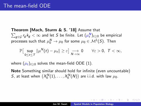
Theorem [Mach, Sturm & S. ’18] Assume that∑g∈G rgkg <∞ and let S be finite. Let (µNt )t≥0 be empirical
processes such that µN0 → µ0 for some µ0 ∈M1(S). Then
P[
sup0≤t≤T
‖µN(t)− µt‖ ≥ ε]−→N→∞
0 ∀ε > 0, T <∞,
where (µt)t≥0 solves the mean-field ODE (1).
Note Something similar should hold for infinite (even uncountable)S , at least when
(XN
0 (1), . . . ,XN0 (N)
)are i.i.d. with law µ0.
Jan M. Swart Spatial Models in Population Biology
The mean-field ODE
Remark We could be more general and also consider maps
Sk 3 (x1, . . . , xk) 7→(g1(x1, . . . , xk), g2(x1, . . . , xk)
)∈ S2,
and similarly with S2 replaced by Sm (m ≥ 1). However, applyingsuch a map with rate r has for the mean-field ODE the same effectas applying the maps g1 and g2 each with rate r .
Also, in our definition of g i,j , we could have chosen j ∈ i1, . . . , ik,e.g. j = i1 always. Again, although this yields a different Markovprocess, for the mean-field ODE this has no effect.
Jan M. Swart Spatial Models in Population Biology
Cooperative branching
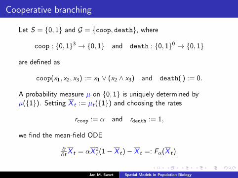
Let S = 0, 1 and G = coop, death, where
coop : 0, 13 → 0, 1 and death : 0, 10 → 0, 1
are defined as
coop(x1, x2, x3) := x1 ∨ (x2 ∧ x3) and death( ) := 0.
A probability measure µ on 0, 1 is uniquely determined byµ(1). Setting X t := µt(1) and choosing the rates
rcoop := α and rdeath := 1,
we find the mean-field ODE
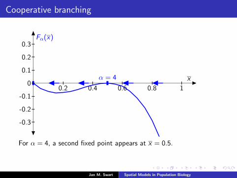
∂∂t X t = αX 2
t (1− X t)− X t =: Fα(X t).
Jan M. Swart Spatial Models in Population Biology
Cooperative branching
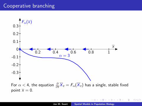
Fα(x)
x
α = 30.2 0.4 0.6 0.8 1
-0.3
-0.2
-0.1
0
0.1
0.2
0.3
For α < 4, the equation ∂∂t X t = Fα(X t) has a single, stable fixed
point x = 0.
Jan M. Swart Spatial Models in Population Biology
Cooperative branching
Fα(x)
xα = 4
0.2 0.4 0.6 0.8 1
-0.3
-0.2
-0.1
0
0.1
0.2
0.3
For α = 4, a second fixed point appears at x = 0.5.
Jan M. Swart Spatial Models in Population Biology
Cooperative branching
Fα(x)
x
α = 5
0.2 0.4 0.6 0.8 1
-0.3
-0.2
-0.1
0
0.1
0.2
0.3
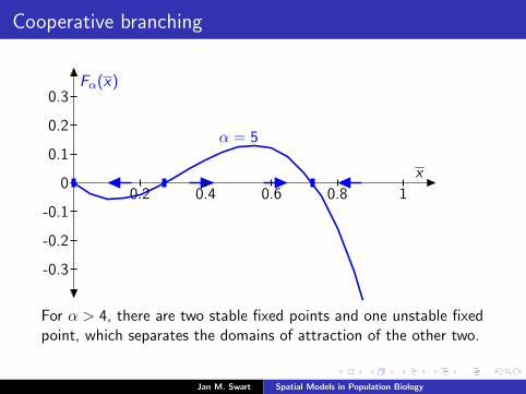
For α > 4, there are two stable fixed points and one unstable fixedpoint, which separates the domains of attraction of the other two.
Jan M. Swart Spatial Models in Population Biology
Cooperative branching
zupp
zmid
zlow
x
α
2 4 6 8 100
0.2
0.4
0.6
0.8
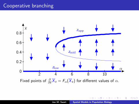
Fixed points of ∂∂t X t = Fα(X t) for different values of α.
Jan M. Swart Spatial Models in Population Biology
Cooperative branching
In physics notation for reaction-diffusion models, cooperativebranching is denoted as 2A 7→ 3A. This sort of dynamics, togetherwith 3A 7→ 2A, was already considered by F. Schlogl [Z. Phys.1972]. Lebowiz, Presutti and Spohn [JSP 1988] call this binaryreproduction.
C. Noble [AOP 1992], R. Durrett [JAP 1992], and C. Neuhauserand S.W. Pacala [AAP 1999] call a model with cooperativebranching and deaths the sexual reproduction process.
The unstable fixed point says that in well-mixing populations, oncethe population drops below a critical level, it becomes so hard fororganisms to find a partner that the population dies out.This effect is also responsible for the first order (discontinuous)phase transition - at least in well-mixing populations.
Jan M. Swart Spatial Models in Population Biology

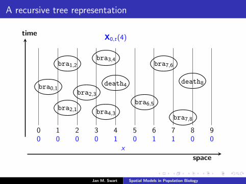
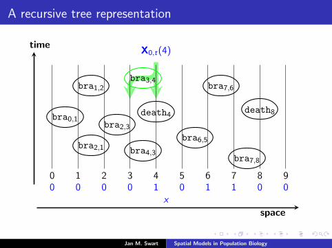
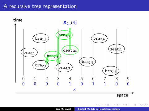
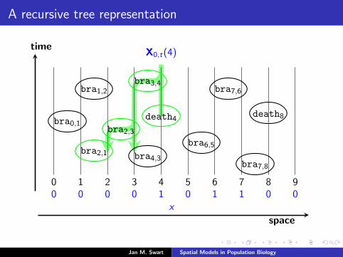
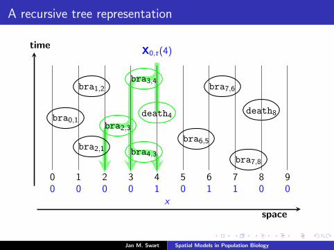
A recursive tree representation
Recall the Markov process(Ri (Xs−t,t))t≥0
that traces back in time all sites at time s − t that are relevant forthe state at the site i at time s.
Jan M. Swart Spatial Models in Population Biology
A recursive tree representation
time
space
0 1 2 3 4 5 6 7 8 90 0 0 0 1 0 1 1 0 0
X0,t(4)
x
bra2,1
bra2,1
bra0,1
bra4,3
bra4,3
bra7,8
bra2,3
bra2,3
death4
death4
bra3,4
bra3,4
bra1,2
bra6,5
bra7,6
death8
Jan M. Swart Spatial Models in Population Biology
A recursive tree representation
time
space
0 1 2 3 4 5 6 7 8 90 0 0 0 1 0 1 1 0 0
X0,t(4)
x
bra2,1
bra2,1
bra0,1
bra4,3
bra4,3
bra7,8
bra2,3
bra2,3
death4
death4
bra3,4
bra3,4bra1,2
bra6,5
bra7,6
death8
Jan M. Swart Spatial Models in Population Biology

A recursive tree representation
time
space
0 1 2 3 4 5 6 7 8 90 0 0 0 1 0 1 1 0 0
X0,t(4)
x
bra2,1
bra2,1
bra0,1
bra4,3
bra4,3
bra7,8
bra2,3
bra2,3
death4
death4
bra3,4
bra3,4bra1,2
bra6,5
bra7,6
death8
Jan M. Swart Spatial Models in Population Biology
A recursive tree representation
time
space
0 1 2 3 4 5 6 7 8 90 0 0 0 1 0 1 1 0 0
X0,t(4)
x
bra2,1
bra2,1
bra0,1
bra4,3
bra4,3
bra7,8
bra2,3
bra2,3
death4
death4
bra3,4
bra3,4bra1,2
bra6,5
bra7,6
death8
Jan M. Swart Spatial Models in Population Biology
A recursive tree representation
time
space
0 1 2 3 4 5 6 7 8 90 0 0 0 1 0 1 1 0 0
X0,t(4)
x
bra2,1
bra2,1
bra0,1
bra4,3
bra4,3
bra7,8
bra2,3
bra2,3
death4
death4
bra3,4
bra3,4bra1,2
bra6,5
bra7,6
death8
Jan M. Swart Spatial Models in Population Biology
A recursive tree representation
time
space
0 1 2 3 4 5 6 7 8 90 0 0 0 1 0 1 1 0 0
X0,t(4)
x
bra2,1
bra2,1
bra0,1
bra4,3
bra4,3bra7,8
bra2,3
bra2,3
death4
death4
bra3,4
bra3,4bra1,2
bra6,5
bra7,6
death8
Jan M. Swart Spatial Models in Population Biology

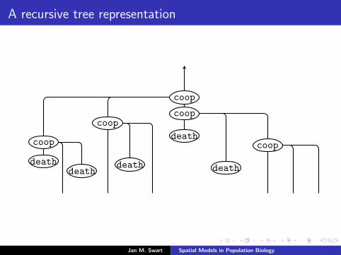
A recursive tree representation
In the mean-field limit, (Ri (Xs−t,t))t≥0
converges to a branching process.
Jan M. Swart Spatial Models in Population Biology
A recursive tree representation
coop
coop
coopcoop
coop
deathdeath
death
death
death
Jan M. Swart Spatial Models in Population Biology
A recursive tree representation
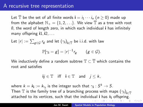
Let T be the set of all finite words i = i1 · · · in (n ≥ 0) made upfrom the alphabet N+ = 1, 2, . . .. We view T as a tree with root∅, the word of length zero, in which each individual i has infinitelymany offspring i1, i2, . . .
Let |r | :=∑
g∈G rg and let (γi)i∈T be i.i.d. with law
P[γi = g ] = |r |−1rg (g ∈ G).
We inductively define a random subtree T ⊂ T which contains theroot and satisfies
ij ∈ T iff i ∈ T and j ≤ k,
where k = ki := kγi is the integer such that γi : Sk → S .Then T is the family tree of a branching process with maps (γi)i∈Tattached to its vertices, such that the individual i has ki offspring.
Jan M. Swart Spatial Models in Population Biology
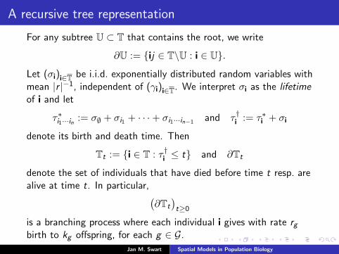
A recursive tree representation
For any subtree U ⊂ T that contains the root, we write
∂U := ij ∈ T\U : i ∈ U.
Let (σi)i∈T be i.i.d. exponentially distributed random variables withmean |r |−1, independent of (γi)i∈T. We interpret σi as the lifetimeof i and let
τ∗i1···in := σ∅ + σi1 + · · ·+ σi1···in−1 and τ †i := τ∗i + σi
denote its birth and death time. Then
Tt := i ∈ T : τ †i ≤ t and ∂Tt
denote the set of individuals that have died before time t resp. arealive at time t. In particular,(
∂Tt
)t≥0
is a branching process where each individual i gives with rate rgbirth to kg offspring, for each g ∈ G.
Jan M. Swart Spatial Models in Population Biology
A recursive tree representation
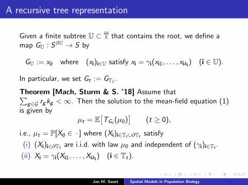
Given a finite subtree U ⊂ T that contains the root, we define amap GU : S∂U → S by
GU := x∅ where (xi)i∈U satisfy xi = γi(xi1, . . . , xiki) (i ∈ U).
In particular, we set Gt := GTt .
Theorem [Mach, Sturm & S. ’18] Assume that∑g∈G rgkg <∞. Then the solution to the mean-field equation (1)
is given byµt = E
[TGt (µ0)
](t ≥ 0),
i.e., µt = P[X∅ ∈ · ] where (Xi)i∈Tt∪∂Tt satisfy
(i) (Xi)i∈∂Tt are i.i.d. with law µ0 and independent of (γi)i∈Tt .
(ii) Xi = γi(Xi1, . . . ,Xiki) (i ∈ Tt).
Jan M. Swart Spatial Models in Population Biology

A recursive tree representation
X∅ law µt
X21
coop
X32
coop
X23
coop
X131
coop
X132 X133i.i.d. µ0
coop
deathdeath
death
death
death
Jan M. Swart Spatial Models in Population Biology
A recursive tree representation
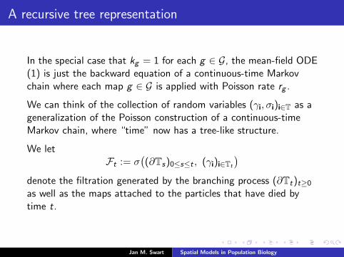
In the special case that kg = 1 for each g ∈ G, the mean-field ODE(1) is just the backward equation of a continuous-time Markovchain where each map g ∈ G is applied with Poisson rate rg .
We can think of the collection of random variables (γi, σi)i∈T as ageneralization of the Poisson construction of a continuous-timeMarkov chain, where “time” now has a tree-like structure.
We letFt := σ
((∂Ts)0≤s≤t , (γi)i∈Tt
)denote the filtration generated by the branching process (∂Tt)t≥0
as well as the maps attached to the particles that have died bytime t.
Jan M. Swart Spatial Models in Population Biology
Unique ergodicity
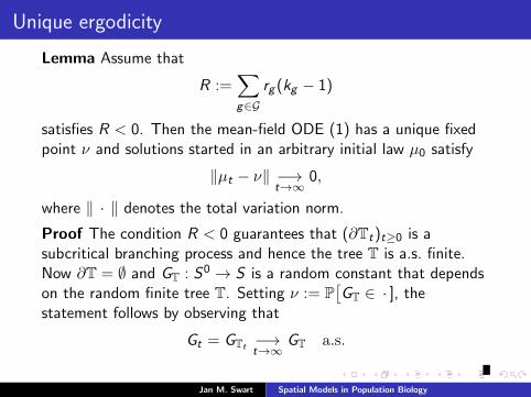
Lemma Assume that
R :=∑g∈G
rg (kg − 1)
satisfies R < 0. Then the mean-field ODE (1) has a unique fixedpoint ν and solutions started in an arbitrary initial law µ0 satisfy
‖µt − ν‖ −→t→∞
0,
where ‖ · ‖ denotes the total variation norm.
Proof The condition R < 0 guarantees that (∂Tt)t≥0 is asubcritical branching process and hence the tree T is a.s. finite.Now ∂T = ∅ and GT : S0 → S is a random constant that dependson the random finite tree T. Setting ν := P
[GT ∈ · ], the
statement follows by observing that
Gt = GTt −→t→∞GT a.s.
Jan M. Swart Spatial Models in Population Biology
Unique ergodicity
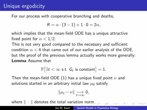
For our process with cooperative branching and deaths,
R = α · (3− 1) + 1 · 0 = 2α,
which implies that the mean-field ODE has a unique attractivefixed point for α < 1/2.This is not very good compared to the necessary and sufficientcondition α < 4 that came out of our earlier analysis of the ODE,but the proof of the previous lemma actually works more generally:Lemma Assume that
P[∃t <∞ s.t. Gt is constant
]= 1.
Then the mean-field ODE (1) has a unique fixed point ν andsolutions started in an arbitrary initial law µ0 satisfy
‖µt − ν‖ −→t→∞
0,
where ‖ · ‖ denotes the total variation norm.Jan M. Swart Spatial Models in Population Biology

Unique ergodicity
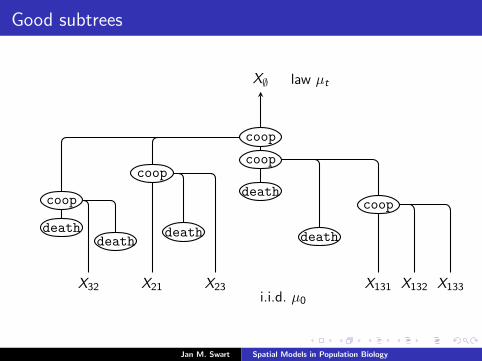
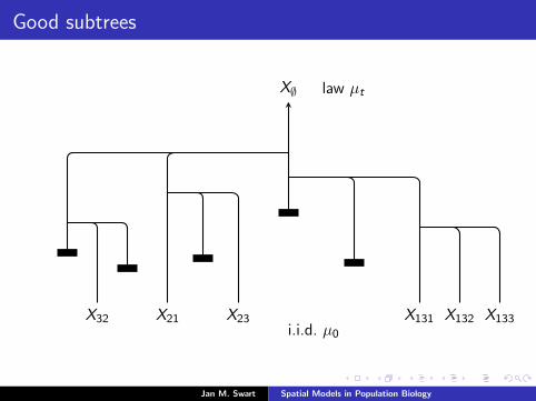
For our process with cooperative branching and deaths, say thatS ⊂ T is a good subtree if ∅ ∈ S and
(i) γi 6= death for all i ∈ S(ii) ∀i ∈ S, i1, i2, i3 ∩ S is either i1 or i2, i3.Lemma The following events are a.s. equal:
(i) T contains a good subtree.
(ii) Gt is constant for some t <∞.
Moreover, P[T contains a good subtree] > 0 iff α ≥ 4.
Jan M. Swart Spatial Models in Population Biology
Good subtrees
X∅ law µt
X21X32 X23 X131 X132 X133i.i.d. µ0
coop
coop
coopcoop
coop
deathdeath
death
death
death
Jan M. Swart Spatial Models in Population Biology
Good subtrees
X∅ law µt
X21X32 X23 X131 X132 X133i.i.d. µ0
Jan M. Swart Spatial Models in Population Biology

Good subtrees
11 1
a good subtree
Jan M. Swart Spatial Models in Population Biology

Good subtrees
11 1
11 1 1dual process Y t
Jan M. Swart Spatial Models in Population Biology

A Recursive Distributional Equation
Fixed points µ of the mean-field ODE (1) solve the RecursiveDistributional Equation (RDE)
µ = |r |−1∑g∈G
Tg (µ). (2)
For each solution µ to the RDE, it is possible to define a collectionof random variables (γi,Xi)i∈T such that:
(i) (γi)i∈T is an i.i.d. collection of G-valued random variables withlaw P[γi = g ] = |r |−1rg (g ∈ G).
(ii) For each finite subtree U ⊂ T that contains the root, (Xi)i∈∂Uare i.i.d. with common law µ and independent of (γi)i∈U.
(iii) Xi = γi(Xi1, . . . ,Xiki) (i ∈ T).
Following Aldous and Bandyopadhyay (2005), we call such acollection of r.v.’s a Recursive Tree Process (RTP).
Jan M. Swart Spatial Models in Population Biology
A Recursive Distributional Equation
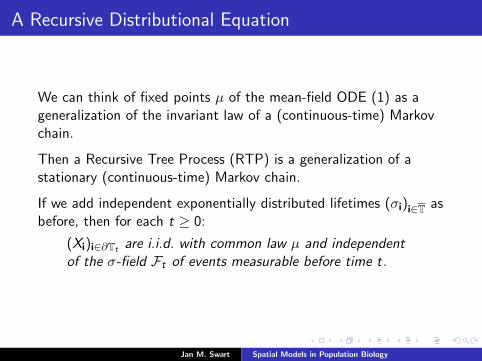
We can think of fixed points µ of the mean-field ODE (1) as ageneralization of the invariant law of a (continuous-time) Markovchain.
Then a Recursive Tree Process (RTP) is a generalization of astationary (continuous-time) Markov chain.
If we add independent exponentially distributed lifetimes (σi)i∈T asbefore, then for each t ≥ 0:
(Xi)i∈∂Tt are i.i.d. with common law µ and independentof the σ-field Ft of events measurable before time t.
Jan M. Swart Spatial Models in Population Biology

The n-variate ODE
Recall that the mean-field ODE (1) describes the Markov process(XN
t )t≥0 on the complete graph in the mean-field limit N →∞.
The Markov process (XNt )t≥0 is defined in terms of a stochastic
flow (XNs,t)s≤t .
The stochastic flow (XNs,t)s≤t contains more information than the
Markov process (XNt )t≥0 alone; in particular, the stochastic flow
provides us with a natural way of coupling processes with differentinitial states.
We would like to understand this coupling in the mean-field limitN →∞.
Jan M. Swart Spatial Models in Population Biology

The n-variate ODE
For each measurable map g : Sk → S and n ≥ 1, we define ann-variate map g (n) : (Sn)k → Sn by
g (n)(x1, . . . , xn) :=
(g(x1), . . . , g(xn)
)(x1, . . . , xn ∈ Sk).
Let G and (rg )g∈G be as before. We will be interested in then-variate ODE
∂∂tµ
(n)t =
∑g∈G
rg
Tg (n)(µ(n)t )− µ(n)
t
(t ≥ 0),
that describes the mean-field limit of n coupled Markov processes,that are constructed from the same stochastic flow but havedifferent initial states.
Jan M. Swart Spatial Models in Population Biology

The n-variate ODE
Let M1sym(Sn) be the space of all probability measures on Sn that
are symmetric under a permutation of the coordinates.For any µ ∈M1(S), let M1
sym(Sn)µ be the set of all symmetric
µ(n) whose one-dimensional marginals are given by µ.Let Sn
diag :=
(x1, . . . , xn) ∈ Sn : x1 = · · · = xn
.
Observations
I If (µ(n)t )t≥0 solves the n-variate ODE, then its m-dimensional
marginals solve the m-variate ODE.
I µ(n)0 ∈M1
sym(Sn) implies µ(n)t ∈M1
sym(Sn) (t ≥ 0).
I If µ(n) solves the n-variate ODE, then µ(n)0 ∈M1
sym(Sn)µ
implies µ(n)t ∈M1
sym(Sn)µ (t ≥ 0).
I If µ(n)0 is concentrated on Sn
diag then so is µ(n)t (t ≥ 0).
Jan M. Swart Spatial Models in Population Biology

The n-variate ODE
In particular, these observations show that if µ(n) solves then-variate RDE, then its marginals must solve the RDE (2).Conversely, if µ solves the RDE (2) and X is a random variablewith law µ, then
µ(n) := P[(X , . . . ,X ) ∈ ·
]solves the n-variate RDE.
Question Are all fixed points of the n-variate RDE of this form?
Jan M. Swart Spatial Models in Population Biology
The bivariate ODE for cooperative branching
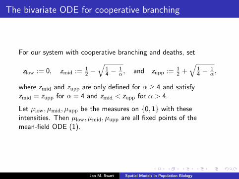
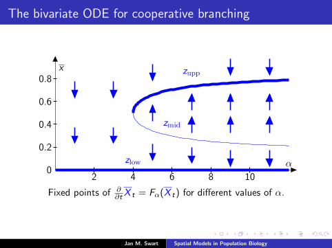
For our system with cooperative branching and deaths, set
zlow := 0, zmid := 12 −
√14 −
1α , and zupp := 1
2 +√
14 −
1α ,
where zmid and zupp are only defined for α ≥ 4 and satisfyzmid = zupp for α = 4 and zmid < zupp for α > 4.
Let µlow, µmid, µupp be the measures on 0, 1 with theseintensities. Then µlow, µmid, µupp are all fixed points of themean-field ODE (1).
Jan M. Swart Spatial Models in Population Biology
The bivariate ODE for cooperative branching
zupp
zmid
zlow
x
α
2 4 6 8 100
0.2
0.4
0.6
0.8
Fixed points of ∂∂t X t = Fα(X t) for different values of α.
Jan M. Swart Spatial Models in Population Biology

The bivariate ODE for cooperative branching
Proposition The measures µ(2)low, µ
(2)mid, µ
(2)upp defined as
µ(2)low := P
[(X ,X ) ∈ ·
]with P[X ∈ · ] = µlow
etc. are fixed points of the bivariate ODE. In addition, for α > 4,
there exists one more fixed point µ(2)mid ∈M
1sym(0, 12) that has
marginals µmid but differs from µ(2)mid.
Any solution (µ(2)t )t≥0 to the bivariate ODE with
µ(2)0 ∈M1
sym(0, 1)µmidand µ
(2)0 6= µ
(2)mid satisfies
µ(2)t =⇒
t→∞µ(2)mid
.
Jan M. Swart Spatial Models in Population Biology
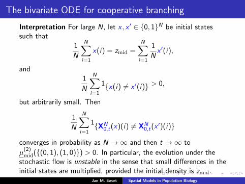
The bivariate ODE for cooperative branching
Interpretation For large N, let x , x ′ ∈ 0, 1N be initial statessuch that
1
N
N∑i=1
x(i) = zmid =N∑i=1
1
Nx ′(i),
and
1
N
N∑i=1
1x(i) 6= x ′(i) > 0,
but arbitrarily small. Then
1
N
N∑i=1
1XN0,t(x)(i) 6= XN
0,t(x ′)(i)
converges in probability as N →∞ and then t →∞ to
µ(2)mid((0, 1), (1, 0)) > 0. In particular, the evolution under the
stochastic flow is unstable in the sense that small differences in theinitial states are multiplied, provided the initial density is zmid.
Jan M. Swart Spatial Models in Population Biology

Endogeny
Aldous and Bandyopadhyay (2005) call a Recursive Tree Process(RTP) (γi,Xi)i∈T endogenous if
X∅ is measurable w.r.t. the σ-field generated by (γi)i∈T.
Theorem [AB ’05, MSS ’18] For any solution µ to the RDE (2),the following statements are equivalent.
(i) The RTP corresponding to µ is endogenous.
(ii) The measure µ(2) is the only solution of the bivariate RDE inthe space M1
sym(S2)µ.
(iii) Solutions to the n-variate ODE satisfy µ(n)t =⇒
t→∞µ(2) for all
µ(n)0 ∈M1
sym(S2)µ and n ≥ 1.
Jan M. Swart Spatial Models in Population Biology

Endogeny
In our example of a system with cooperative branching and deaths,the RTPs corresponding to µlow and µupp are endogenous, but forα > 4, the RTP corresponding to µmid is not endogenous.
Proposition [AB ’05] Let S be a finite partially ordered set withminimal and maximal elements 0, 1. Assume that all maps m ∈ Gare monotone. Let (µ0
t )t≥0 and (µ1t )t≥0 be solutions to the
mean-field ODE with initial states µ00 = δ0 and µ1
0 = δ1. Thenthere exist solutions ν and ν to the RDE (2) such that
µ0t =⇒t→∞
ν and µ1t =⇒t→∞
ν.
Moreover, the RTPs corresponding to ν and ν are endogenous.
Jan M. Swart Spatial Models in Population Biology
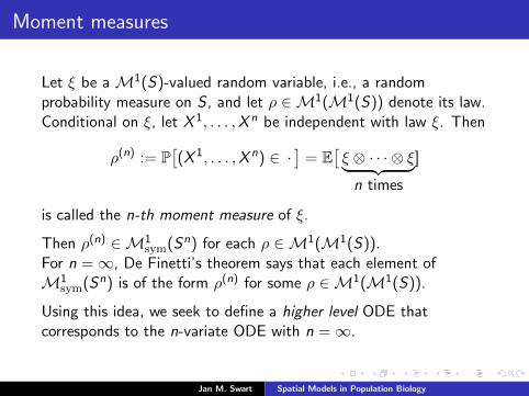
Moment measures
Let ξ be a M1(S)-valued random variable, i.e., a randomprobability measure on S , and let ρ ∈M1(M1(S)) denote its law.Conditional on ξ, let X 1, . . . ,X n be independent with law ξ. Then
ρ(n) := P[(X 1, . . . ,X n) ∈ ·
]= E
[ξ ⊗ · · · ⊗ ξ︸ ︷︷ ︸
n times
]
is called the n-th moment measure of ξ.
Then ρ(n) ∈M1sym(Sn) for each ρ ∈M1(M1(S)).
For n =∞, De Finetti’s theorem says that each element ofM1
sym(Sn) is of the form ρ(n) for some ρ ∈M1(M1(S)).
Using this idea, we seek to define a higher level ODE thatcorresponds to the n-variate ODE with n =∞.
Jan M. Swart Spatial Models in Population Biology

The higher-level ODE
Recall that for each measurable map g : Sk → S , we have defineda measurable map g :M1(S)k →M1(S) by
g(µ1, . . . , µk) := P[g(X1, . . . ,Xk) ∈ ·
]where X1, . . . ,Xk are indep. with P[Xi ∈ · ] = µi .
In particular, Tg :M1(S)→M1(S) is defined by
Tg (µ) := g(µ, . . . , µ).
The higher level ODE is the equation
∂∂t ρt =
∑g∈G
Tg (ρt)− ρt
(t ≥ 0).
This differs from the mean-field ODE (1) in the sense that Tg isreplaced by Tg and ρt takes values in M1(M1(S)).
Jan M. Swart Spatial Models in Population Biology

The higher-level ODE
Lemma If (ρt)t≥0 solves the higher level ODE, then its n-thmoment measures solve the n-variate ODE.
Below, we equip the space M1(M1(S))µ of all ρ ∈M1(M1(S))with first moment measure ρ(1) = µ with the convex orderρ1 ≤cv ρ2, defined as∫
φ dρ1 ≤∫φ dρ2 ∀ convex bounded contin. φ :M1(S)→ R.
Theorem [MSS ’18] Let µ be a fixed point of the mean-fieldODE (1). Then the higher-level ODE has fixed pointsµ, µ ∈M1(M1(S))µ that are minimal and maximal with respectto the convex order.Remark One has ρ1 ≤cv ρ2 iff there exists an S-valued randomvariable X on some probability space (Ω,F ,P) and sub-σ-fieldsF1 ⊂ F2 ⊂ F such that ρi = P
[P[X ∈ · |Fi ] ∈ ·
](i = 1, 2).
Jan M. Swart Spatial Models in Population Biology

The higher-level ODE
Theorem [MSS ’18] Let µ be a fixed point of the mean-fieldODE (1). Let (γi,Xi)i∈T be the RTP corresponding to µ. Set
ξi := P[Xi ∈ · | (γij)j∈T
].
Then(γi, ξi)i∈T and (γi, δXi
)i∈T
are RTPs corresponding to the fixed points µ, µ of the higher-levelODE. The original RTP is endogenous if and only if µ = µ.
Remark 1 µ and µ correspond to minimal and maximal knowledgeabout X∅. The former describes the knowledge contained in(γi)i∈T, the latter represents perfect knowledge.
Remark 2 µ(n) := P[(X , . . . ,X ) ∈ ·
]in line with earlier notation.
Jan M. Swart Spatial Models in Population Biology

The higher-level ODE
In our example of a system with cooperative branching and deaths,we identify
M1(0, 1) 3 µ 7→ µ(1) ∈ [0, 1]
and correspondingly M1(M1(0, 1)) ∼=M1[0, 1]. If g = coop,then g : [0, 1]3 → [0, 1] is given by
g(ω1, ω2, ω3) := P[X1 ∨ (X2 ∧ X3) = 1] with P[Xi = 1] = ωi ,
which gives
g(ω1, ω2, ω3) = ω1 + (1− ω1)ω2ω3
and, for any ρ ∈M1[0, 1],
Tg (ρ) = P[ω1+(1−ω1)ω2ω3 ∈ ·
]with ω1, ω2, ω3 i.i.d. with law ρ.
Jan M. Swart Spatial Models in Population Biology

The higher-level ODE
Proposition For our system with cooperative branching anddeaths, for α > 4, the higher-level ODE
∂∂t ρt = α
Tg (ρ)− ρ
+δ0 − ρ
has precisely four fixed points. Three trivial fixed points of the form
ρ = (1− z)δ0 + zδ1 with z = zlow, zmid, zupp,
and a nontrivial fixed point µmid
which is the law of the[0, 1]-valued random variable
P[X∅ = 1
∣∣ (γi)i∈T]
where (γi,Xi)i∈T is the RTP with P[X∅ = 1] = zmid.
Jan M. Swart Spatial Models in Population Biology

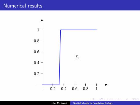
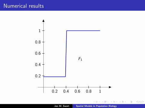
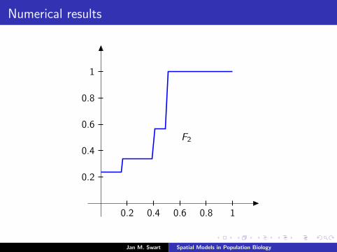
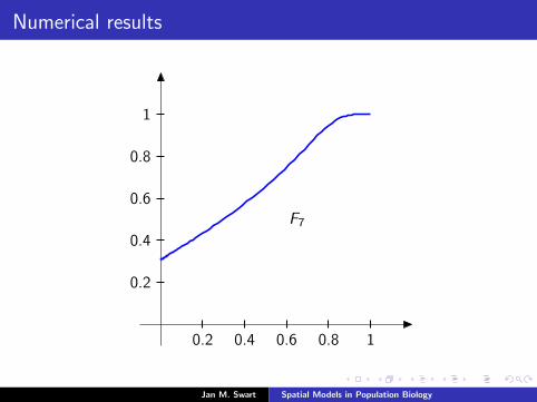
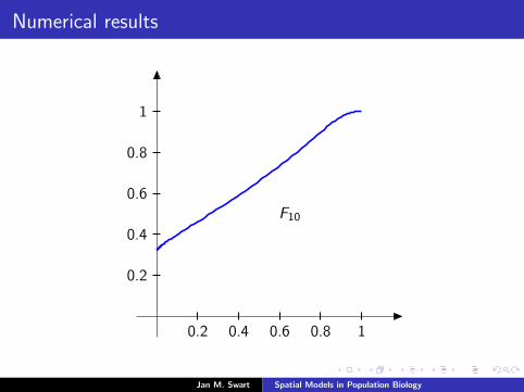
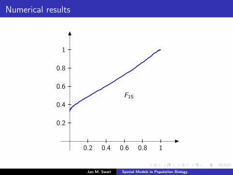
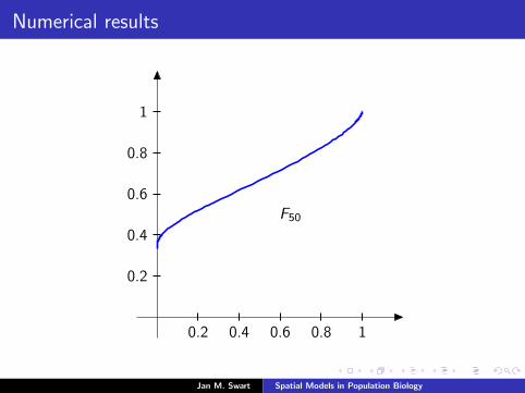
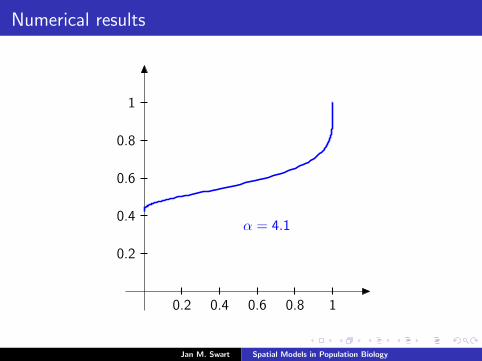
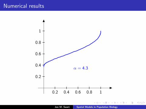
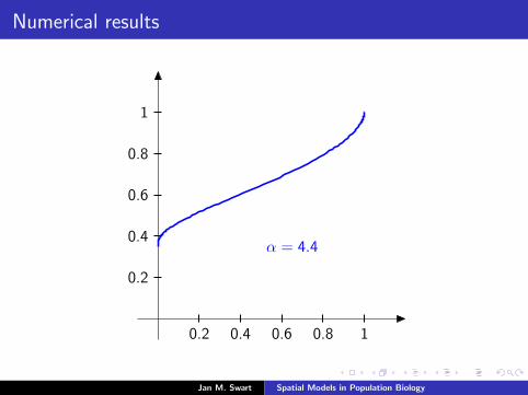
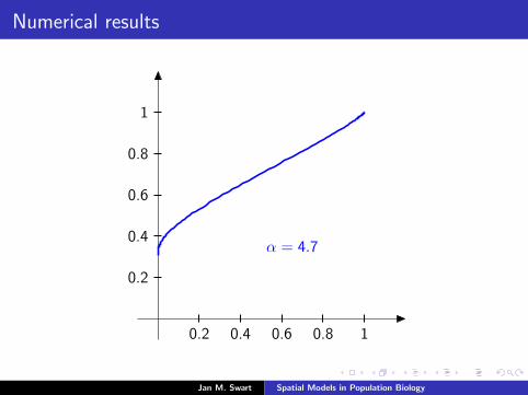
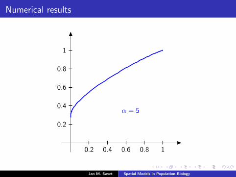
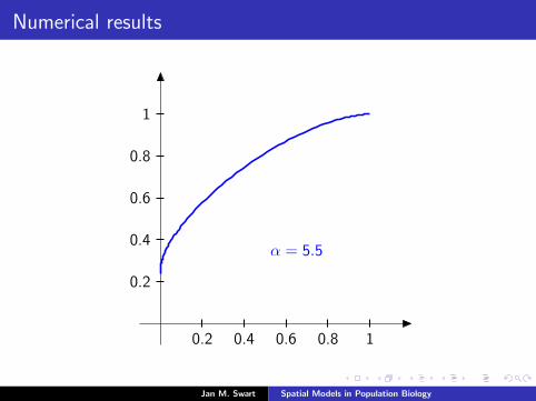
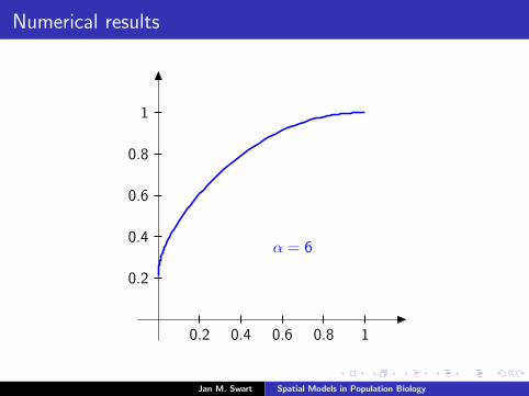
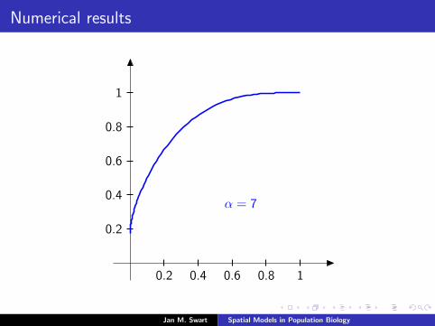
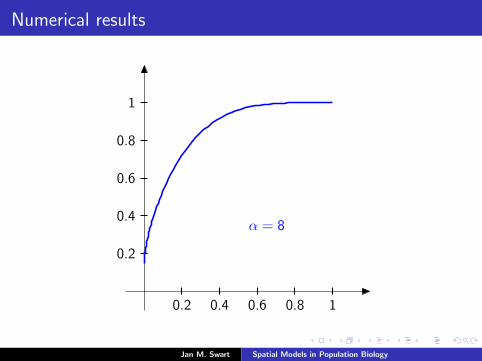
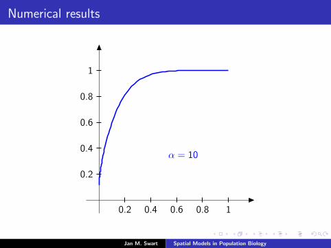
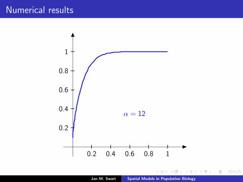
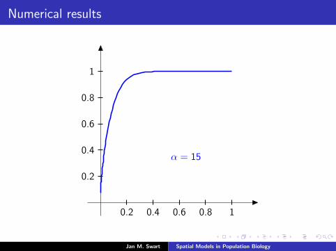
Numerical results
The measure µmid
should be the limit of measures µn inductivelydefined as µ0 = δzmid
and
µn =α
α + 1Tg (µn−1) +
1
α + 1δ0.
We plot the distribution functions
Fn(s) := µn([0, s]
) (s ∈ [0, 1]
)for the parameters α = 9/2, zmid = 1/3, zupp = 2/3 and variousvalues of n.
Jan M. Swart Spatial Models in Population Biology
Numerical results
0.2 0.4 0.6 0.8 1
0.2
0.4
0.6
0.8
1
F0
F1F2F3F4F5F7F10F15F25F50F100
α = 4.1α = 4.2α = 4.3α = 4.4α = 4.5α = 4.7α = 5α = 5.5α = 6α = 7α = 8α = 10α = 12α = 15
Jan M. Swart Spatial Models in Population Biology
Numerical results
0.2 0.4 0.6 0.8 1
0.2
0.4
0.6
0.8
1
F0
F1
F2F3F4F5F7F10F15F25F50F100
α = 4.1α = 4.2α = 4.3α = 4.4α = 4.5α = 4.7α = 5α = 5.5α = 6α = 7α = 8α = 10α = 12α = 15
Jan M. Swart Spatial Models in Population Biology
Numerical results
0.2 0.4 0.6 0.8 1
0.2
0.4
0.6
0.8
1
F0F1
F2
F3F4F5F7F10F15F25F50F100
α = 4.1α = 4.2α = 4.3α = 4.4α = 4.5α = 4.7α = 5α = 5.5α = 6α = 7α = 8α = 10α = 12α = 15
Jan M. Swart Spatial Models in Population Biology

Numerical results
0.2 0.4 0.6 0.8 1
0.2
0.4
0.6
0.8
1
F0F1F2
F3
F4F5F7F10F15F25F50F100
α = 4.1α = 4.2α = 4.3α = 4.4α = 4.5α = 4.7α = 5α = 5.5α = 6α = 7α = 8α = 10α = 12α = 15
Jan M. Swart Spatial Models in Population Biology

Numerical results
0.2 0.4 0.6 0.8 1
0.2
0.4
0.6
0.8
1
F0F1F2F3
F4
F5F7F10F15F25F50F100
α = 4.1α = 4.2α = 4.3α = 4.4α = 4.5α = 4.7α = 5α = 5.5α = 6α = 7α = 8α = 10α = 12α = 15
Jan M. Swart Spatial Models in Population Biology

Numerical results
0.2 0.4 0.6 0.8 1
0.2
0.4
0.6
0.8
1
F0F1F2F3F4
F5
F7F10F15F25F50F100
α = 4.1α = 4.2α = 4.3α = 4.4α = 4.5α = 4.7α = 5α = 5.5α = 6α = 7α = 8α = 10α = 12α = 15
Jan M. Swart Spatial Models in Population Biology
Numerical results
0.2 0.4 0.6 0.8 1
0.2
0.4
0.6
0.8
1
F0F1F2F3F4F5
F7
F10F15F25F50F100
α = 4.1α = 4.2α = 4.3α = 4.4α = 4.5α = 4.7α = 5α = 5.5α = 6α = 7α = 8α = 10α = 12α = 15
Jan M. Swart Spatial Models in Population Biology
Numerical results
0.2 0.4 0.6 0.8 1
0.2
0.4
0.6
0.8
1
F0F1F2F3F4F5F7
F10
F15F25F50F100
α = 4.1α = 4.2α = 4.3α = 4.4α = 4.5α = 4.7α = 5α = 5.5α = 6α = 7α = 8α = 10α = 12α = 15
Jan M. Swart Spatial Models in Population Biology
Numerical results
0.2 0.4 0.6 0.8 1
0.2
0.4
0.6
0.8
1
F0F1F2F3F4F5F7F10
F15
F25F50F100
α = 4.1α = 4.2α = 4.3α = 4.4α = 4.5α = 4.7α = 5α = 5.5α = 6α = 7α = 8α = 10α = 12α = 15
Jan M. Swart Spatial Models in Population Biology

Numerical results
0.2 0.4 0.6 0.8 1
0.2
0.4
0.6
0.8
1
F0F1F2F3F4F5F7F10F15
F25
F50F100
α = 4.1α = 4.2α = 4.3α = 4.4α = 4.5α = 4.7α = 5α = 5.5α = 6α = 7α = 8α = 10α = 12α = 15
Jan M. Swart Spatial Models in Population Biology
Numerical results
0.2 0.4 0.6 0.8 1
0.2
0.4
0.6
0.8
1
F0F1F2F3F4F5F7F10F15F25
F50
F100
α = 4.1α = 4.2α = 4.3α = 4.4α = 4.5α = 4.7α = 5α = 5.5α = 6α = 7α = 8α = 10α = 12α = 15
Jan M. Swart Spatial Models in Population Biology

Numerical results
0.2 0.4 0.6 0.8 1
0.2
0.4
0.6
0.8
1
F0F1F2F3F4F5F7F10F15F25F50
F100
α = 4.1α = 4.2α = 4.3α = 4.4α = 4.5α = 4.7α = 5α = 5.5α = 6α = 7α = 8α = 10α = 12α = 15
Jan M. Swart Spatial Models in Population Biology
Numerical results
0.2 0.4 0.6 0.8 1
0.2
0.4
0.6
0.8
1
F0F1F2F3F4F5F7F10F15F25F50F100
α = 4.1
α = 4.2α = 4.3α = 4.4α = 4.5α = 4.7α = 5α = 5.5α = 6α = 7α = 8α = 10α = 12α = 15
Jan M. Swart Spatial Models in Population Biology

Numerical results
0.2 0.4 0.6 0.8 1
0.2
0.4
0.6
0.8
1
F0F1F2F3F4F5F7F10F15F25F50F100
α = 4.1
α = 4.2
α = 4.3α = 4.4α = 4.5α = 4.7α = 5α = 5.5α = 6α = 7α = 8α = 10α = 12α = 15
Jan M. Swart Spatial Models in Population Biology
Numerical results
0.2 0.4 0.6 0.8 1
0.2
0.4
0.6
0.8
1
F0F1F2F3F4F5F7F10F15F25F50F100
α = 4.1α = 4.2
α = 4.3
α = 4.4α = 4.5α = 4.7α = 5α = 5.5α = 6α = 7α = 8α = 10α = 12α = 15
Jan M. Swart Spatial Models in Population Biology
Numerical results
0.2 0.4 0.6 0.8 1
0.2
0.4
0.6
0.8
1
F0F1F2F3F4F5F7F10F15F25F50F100
α = 4.1α = 4.2α = 4.3
α = 4.4
α = 4.5α = 4.7α = 5α = 5.5α = 6α = 7α = 8α = 10α = 12α = 15
Jan M. Swart Spatial Models in Population Biology

Numerical results
0.2 0.4 0.6 0.8 1
0.2
0.4
0.6
0.8
1
F0F1F2F3F4F5F7F10F15F25F50F100
α = 4.1α = 4.2α = 4.3α = 4.4
α = 4.5
α = 4.7α = 5α = 5.5α = 6α = 7α = 8α = 10α = 12α = 15
Jan M. Swart Spatial Models in Population Biology
Numerical results
0.2 0.4 0.6 0.8 1
0.2
0.4
0.6
0.8
1
F0F1F2F3F4F5F7F10F15F25F50F100
α = 4.1α = 4.2α = 4.3α = 4.4α = 4.5
α = 4.7
α = 5α = 5.5α = 6α = 7α = 8α = 10α = 12α = 15
Jan M. Swart Spatial Models in Population Biology
Numerical results
0.2 0.4 0.6 0.8 1
0.2
0.4
0.6
0.8
1
F0F1F2F3F4F5F7F10F15F25F50F100
α = 4.1α = 4.2α = 4.3α = 4.4α = 4.5α = 4.7
α = 5
α = 5.5α = 6α = 7α = 8α = 10α = 12α = 15
Jan M. Swart Spatial Models in Population Biology
Numerical results
0.2 0.4 0.6 0.8 1
0.2
0.4
0.6
0.8
1
F0F1F2F3F4F5F7F10F15F25F50F100
α = 4.1α = 4.2α = 4.3α = 4.4α = 4.5α = 4.7α = 5
α = 5.5
α = 6α = 7α = 8α = 10α = 12α = 15
Jan M. Swart Spatial Models in Population Biology
Numerical results
0.2 0.4 0.6 0.8 1
0.2
0.4
0.6
0.8
1
F0F1F2F3F4F5F7F10F15F25F50F100
α = 4.1α = 4.2α = 4.3α = 4.4α = 4.5α = 4.7α = 5α = 5.5
α = 6
α = 7α = 8α = 10α = 12α = 15
Jan M. Swart Spatial Models in Population Biology
Numerical results
0.2 0.4 0.6 0.8 1
0.2
0.4
0.6
0.8
1
F0F1F2F3F4F5F7F10F15F25F50F100
α = 4.1α = 4.2α = 4.3α = 4.4α = 4.5α = 4.7α = 5α = 5.5α = 6
α = 7
α = 8α = 10α = 12α = 15
Jan M. Swart Spatial Models in Population Biology
Numerical results
0.2 0.4 0.6 0.8 1
0.2
0.4
0.6
0.8
1
F0F1F2F3F4F5F7F10F15F25F50F100
α = 4.1α = 4.2α = 4.3α = 4.4α = 4.5α = 4.7α = 5α = 5.5α = 6α = 7
α = 8
α = 10α = 12α = 15
Jan M. Swart Spatial Models in Population Biology
Numerical results
0.2 0.4 0.6 0.8 1
0.2
0.4
0.6
0.8
1
F0F1F2F3F4F5F7F10F15F25F50F100
α = 4.1α = 4.2α = 4.3α = 4.4α = 4.5α = 4.7α = 5α = 5.5α = 6α = 7α = 8
α = 10
α = 12α = 15
Jan M. Swart Spatial Models in Population Biology
Numerical results
0.2 0.4 0.6 0.8 1
0.2
0.4
0.6
0.8
1
F0F1F2F3F4F5F7F10F15F25F50F100
α = 4.1α = 4.2α = 4.3α = 4.4α = 4.5α = 4.7α = 5α = 5.5α = 6α = 7α = 8α = 10
α = 12
α = 15
Jan M. Swart Spatial Models in Population Biology
Numerical results
0.2 0.4 0.6 0.8 1
0.2
0.4
0.6
0.8
1
F0F1F2F3F4F5F7F10F15F25F50F100
α = 4.1α = 4.2α = 4.3α = 4.4α = 4.5α = 4.7α = 5α = 5.5α = 6α = 7α = 8α = 10α = 12
α = 15
Jan M. Swart Spatial Models in Population Biology