it s not factor accumulation: stylized facts and growth models...it s not factor accumulation:...
TRANSCRIPT

177
© 2001 The International Bank for Reconstruction and Development / THE WORLD BANK
the world bank economic review, vol. 15, no. 2 177–219
It’s Not Factor Accumulation:Stylized Facts and Growth Models
William Easterly and Ross Levine
The article documents five stylized facts of economic growth. (1) The “residual” (totalfactor productivity, tfp) rather than factor accumulation accounts for most of the in-come and growth differences across countries. (2) Income diverges over the long run.(3) Factor accumulation is persistent while growth is not, and the growth path of coun-tries exhibits remarkable variation. (4) Economic activity is highly concentrated, withall factors of production flowing to the richest areas. (5) National policies are closelyassociated with long-run economic growth rates. These facts do not support modelswith diminishing returns, constant returns to scale, some fixed factor of production,or an emphasis on factor accumulation. However, empirical work does not yet deci-sively distinguish among the different theoretical conceptions of tfp growth. Econo-mists should devote more effort toward modeling and quantifying tfp.
The central problem in understanding economic development and growth is notunderstanding the process by which an economy raises its savings rate and in-creases the rate of physical capital accumulation.1 Although many developmentpractitioners and researchers continue to target capital accumulation as the driv-
William Easterly is senior advisor, Development Research Group, at the World Bank. His e-mailaddress is [email protected]. Ross Levine is with the University of Minnesota. His e-mail ad-dress is [email protected]. The authors are grateful to Lant Pritchett, who shaped the paper, gavecomments, and provided many of the “stylized facts.” They also thank François Bourguignon, AshokDhareshwar, Robert G. King, Michael Kremer, Peter Klenow, Paul Romer, Xavier Sala-i-Martin, Rob-ert Solow, Albert Zeufack, two anonymous referees, and students and faculty at the Economics Educa-tion Research Consortium program in Kiev, Ukraine, Harvard University’s Kennedy School of Govern-ment, and Johns Hopkins School of Advanced International Studies for useful comments. An earlierversion of this article was presented at the World Bank conference “What Have We Learned from aDecade of Empirical Research on Growth?” held on 26 February 2001.
1. This is a reversal and slight rewording of Arthur Lewis’s (1954, p. 155) famous quote, “Thecentral problem in the theory of economic development is to understand the process by which a com-munity which was previously saving and investing 4 or 5 percent of its national income or less, con-verts itself into an economy where voluntary saving is running at about 12 to 15 percent of nationalincome or more. This is the central problem because the central fact of development is rapid capitalaccumulation (including knowledge and skills with capital).” Though Lewis recognizes the impor-tance of knowledge and skills and later in his book highlights the importance of institutions, manydevelopment economists who followed Lewis adopted the more limited focus on savings and physi-cal capital accumulation.
What have we learned from a decade of empirical research on growth?
Pub
lic D
iscl
osur
e A
utho
rized
Pub
lic D
iscl
osur
e A
utho
rized
Pub
lic D
iscl
osur
e A
utho
rized
Pub
lic D
iscl
osur
e A
utho
rized

178 the world bank economic review, vol. 15, no. 2
ing force in economic growth,2 “something else” besides capital accumulationis critical for understanding differences in economic growth and income acrosscountries. This conclusion is based on evidence on the sources of economicgrowth, the patterns of economic growth, the patterns of factor flows, and theimpact of national policies on economic growth.
This study does not argue that factor accumulation is unimportant in generalor deny that it is critically important for some countries at specific junctures. AsRobert Solow noted in 1956, economists construct models to reproduce crucialempirical regularities and then use these models to interpret economic events andmake policy recommendations. This article documents important empirical regu-larities about economic growth with the hope of highlighting productive direc-tions for future research and improving public policy.
I. Something Else
A growing body of research suggests that, even after physical and human capi-tal accumulation are accounted for, something else accounts for the bulk of cross-country differences in the level and growth rate of gross domestic product (gdp)per capita. Economists typically refer to the something else as total factor pro-ductivity (tfp). This article follows that convention.
Different theories offer very different conceptions of tfp. These range fromchanges in technology (the instructions for producing goods and services) to therole of externalities, changes in the sector composition of production, and theadoption of lower-cost production methods. Evidence that confidently assesseshow well these conceptions of tfp explain economic growth is lacking. Econo-mists need to provide much more shape and substance to the amorphous termtfp, distinguishing empirically among these different theories.
This article examines five stylized facts that illuminate tfp and its determi-nants to enable more precise modeling of long-run economic growth and thedesign of appropriate policies.
2. Academic researchers in the 1990s started a “neoclassical revival” (in the words of Klenow andRodriguez-Clare 1997b). The classic works in the academic literature’s stress on factor accumulationwere Mankiw, Romer, and Weil (1992); Barro and others (1995); Mankiw (1995); and Young (1995).The summary of the Global Development Network conference in Prague in June 2000, representingmany international organizations and development research institutes, says “physical capital accumu-lation was found to be the dominant source of growth both within and across regions. Total factorproductivity growth (TFPG) was not as important as was previously believed” (www.gdnet.org/pdfs/GRPPragueMtgReport.pdf). A leading development textbook (Todaro 2000) says that an increase ininvestment is “a necessary condition” for economic takeoff. The development textbook of Ray (1998,p. 54) refers to investment and saving as “the foundations of all models of economic growth.” Manydevelopment practitioners also stress investment. For example, the International Monetary Fund(Hadjimichael and others 1996, p. 1) argues, “The adjustment experience of sub-Saharan Africa hasdemonstrated that to achieve gains in real per capita GDP an expansion in private saving and investmentis key.” The Bank for International Settlements (1996, p. 50) concludes, “Recent experience has under-lined the central importance of national saving and investment rates in promoting growth.” And theInternational Labor Organization (1995, p. 12) argues that “policies to raise the rate of investment . . .

Easterly and Levine 179
• Stylized fact 1. Factor accumulation does not account for the bulk of cross-country differences in the level or growth rate of gdp per capital; somethingelse—tfp—does. In the search for the secrets of long-run economic growth,a high priority should go to rigorously defining tfp, empirically dissectingit, and identifying the policies and institutions most conducive to its growth.
• Stylized fact 2. There are huge and growing differences in gdp per capita;divergence—not conditional convergence—is the big story. An emphasison tfp growth with increasing returns to technology is more consistent withdivergence than are models of factor accumulation with decreasing returns,no scale economies, and some fixed factor of production. Over the pasttwo centuries, the big story has been the widening difference between therichest and the poorest countries. Moreover, the growth rates of the richare not slowing, and returns to capital are not falling. Just as business cycleslook like little wiggles around the big story when viewed over a long hori-zon, understanding slow, intermittent conditional convergence seems lessintriguing than uncovering why the United States has enjoyed steady growthfor 200 years while much of world still lives in poverty.
• Stylized fact 3. Growth is not persistent over time, but capital accumulationis. Some countries take off, others experience peaks and valleys, a few growsteadily, and some have never grown. Changes in factor accumulation donot closely track changes in economic growth. This finding is consistent acrossvery different frequencies of data. Tangentially, but critically, this stylizedfact also suggests that models of steady-state growth, whether based on capitalexternalities or technological spillovers, will not capture the experiences ofmany countries. While steady-state growth models may fit U.S. experienceover the past 200 years, these models will not fit the experiences of Argen-tina, the Republic of Korea, Thailand, or Venezuela very well. In contrast,models of multiple equilibria do not fit the U.S. data very well. Thus modelstend to be country-specific rather than general theories. Meanwhile, empiri-cal work is still going on to explain why the United States is different, how
are critical for raising the rate of growth and employment in an economy.” Finally “additional invest-ment is the answer—or part of the answer—to most policy problems in the economic and social arena”(United Nations 1996, p. 8). Similarly, the World Bank (1993, p. 191) states that in East Asia, “accu-mulation of productive assets is the foundation of economic growth.” World Bank (1995, p. 10, 23)promises that in Latin America “enhancing saving and investment by 8 percentage points of GDP wouldraise the annual growth figure by around 2 percentage points.” The World Bank (2000a, p. 10) saysthe saving rate of the typical African country “is far below what is needed to sustain a long-term boostin economic performance.” The World Bank (2000c, p. 1) says that southeastern Europe can seize tradeopportunities only if “domestic and foreign entrepreneurs increase their investment dramatically.” Formore citations, see Easterly (1999a) and King and Levine (1994). Although common, the stress on capitalaccumulation is far from universal among development practitioners and researchers. For example, theWorld Bank (2000b, p. 4) report on East Asia’s recovery suggests that “future growth hinges less onincreasing physical capital accumulation and more on raising the productivity growth of all factors.”Collier, Dollar, and Stern (2000) stress policies, incentives, institutions, and exogenous factors as themain drivers in growth with little mention of investment, as does World Development Report 2000/2001 (World Bank 2000/2001, pp. 49–52).

180 the world bank economic review, vol. 15, no. 2
Argentina can go from being like the United States early in this century tothe struggling middle-income country it is today, and how Korea or Thai-land can go from being like Somalia to having thriving economies.
• Stylized fact 4. All factors of production flow to the same places, suggestingimportant externalities. Although this has been noted and modeled by Lucas(1988), Kremer (1993), and others, this article further demonstrates the per-vasive tendency for all factors of production, including physical and humancapital, to bunch together. As a consequence, economic activity is highlyconcentrated. This tendency holds whether considering the world, countries,regions, states, ethnic groups, or cities. Thus the something else that accountsfor the bulk of differences in growth across these units needs to be fleshedout and given a prominent position in theories and policy recommendations.
• Stylized fact 5. National policies influence long-run growth. In models withzero productivity growth, diminishing returns to factors of production, andsome fixed factor, national policies that boost physical or human capitalaccumulation have only a transitional effect on growth. In models thatemphasize tfp growth, national policies that enhance the efficiency of capitaland labor or alter the endogenous rate of technological change can boostproductivity growth and accelerate long-run economic growth. Thus thefinding that policy influences growth is consistent with theories that em-phasize productivity growth and technological externalities and cast increas-ing doubt on theories that focus excessively on factor accumulation.
Although many economists have examined tfp growth and assessed growthmodels, this article makes several new contributions. Besides conducting tradi-tional growth accounting with new Penn-World Table 5.6 capital stock data,this article fully exploits the panel nature of the data. Using an international cross-section of countries, it addresses two questions:
• What accounts for cross-country growth differences?• What accounts for growth differences over time?
Overwhelmingly the answer is tfp, not factor accumulation.The article also examines differences in the level of gdp per worker across
countries. It updates Denison’s (1962) original level accounting study and ex-tends Mankiw, Romer, and Weil’s (1992) study by allowing technology to dif-fer across countries and by assessing the importance of country-specific effects.Unlike Mankiw, Romer, and Weil (1992), it finds that large differences in tfpaccount for the bulk of cross-country differences in income per capita, evencontrolling for country-specific effects.
The article also compiles new information documenting massive divergence inthe level of income per capita across countries. Although many studies base theirmodeling strategies on the U.S. experience of steady long-run growth (see, for ex-ample, Jones 1995a, 1995b; and Rebelo and Stokey 1995), the U.S. experience isthe exception. In much of the world miracles and disasters and changing long-run

Easterly and Levine 181
growth rates are the rule, not stable long-run growth rates. Finally, the article pre-sents abundant new evidence on the concentration of economic activity, drawingon cross-country information, county-level data for the United States, developingcountry studies, and information on the international flow of capital, labor, andhuman capital to demonstrate the geographic concentration of activity and relatethis to models of economic growth. The overwhelming concentration of economicactivity is consistent with some theories of economic growth and inconsistent withothers. Though individual countries at specific points in their development fit dif-ferent models of growth, the big picture emerging from cross-country growth com-parisons is that creating the incentives for productive factor accumulation is moreimportant for growth than factor accumulation itself.
II. Stylized Fact 1. It’s Not Factor Accumulation, It’s tfp
Although physical and human capital accumulation may play key roles in ignitingand accounting for economic progress in some countries, something else—tfp—accounts for the bulk of cross-country differences in the level and growth of gdpper capita in a broad cross-section of countries. The empirical importance of tfphas motivated economists to develop models of tfp. These focus variously on tech-nological change (Aghion and Howitt 1998; Grossman and Helpman 1991; Romer1990); impediments to adopting new technologies (Parente and Prescott 1996);externalities (Romer 1986; Lucas 1988); sectoral development (Kongsamut,Rebelo, and Xie 1997); or cost reductions (Harberger 1998).
This section briefly presents evidence on factor accumulation and growth anddiscusses the implications for models and policy. It considers three questions.First, what part of a country’s growth rate is accounted for by factor accumula-tion and tfp growth? Looking at the sources of growth in individual countriesover time helps answer this question. Second, what part of cross-country differ-ences in economic growth rates is accounted for by cross-country differences ingrowth rates of factor accumulation and tfp? Third, what part of the inter-temporal difference in economic growth rates is accounted for by time-seriesdifferences in growth rates of factor accumulation and tfp? Traditional growthaccounting forms the basis for answering these questions.
Growth Accounting
The organizing principle of growth accounting is the Cobb-Douglas aggregateproduction function:
(1) y = Aka(n1–a),
where y is national output per person,3 A is technological progress, k is the physi-cal capital stock per person, n is the number of units of labor input per person
3. We switch between output per worker and output per person depending on data availability andwhat’s appropriate for each usage.

182 the world bank economic review, vol. 15, no. 2
(reflecting work patterns, human capital, and the like), and a is a productionfunction parameter (equal to the share of capital income in national output underperfect competition).
Output growth is then divided into components attributable to changes in thefactors of production. Rewriting equation 1 in growth rates:
(2) (Dy / y) = (DA / A) + a(Dk / k) + (1 – a)(Dn / n).
Consider a hypothetical country with a growth rate of output per person of2 percent, growth in capital per capita of 3 percent, growth in human capital of0, and capital’s share of national income of 40 percent (a = 0.4). In this example,tfp growth is 0.8 percent, and therefore, tfp-growth accounts for 40 percent(0.8/2) of output growth in this country.
Detailed growth accounting. Many researchers conduct detailed growth ac-counting exercises of one or a few countries, using disaggregated data on capi-tal, labor, human capital, and capital shares of income. Early, detailed growthaccounting exercises of a few countries by Solow (1957) and Denison (1962,1967) found that the rate of capital accumulation per person accounted for be-tween one-eighth and one-fourth of gdp growth rates in the United States andother industrialized countries, whereas tfp-growth accounted for more than halfof gdp growth in many countries.
Subsequent studies showed that it is important to account for changes in thequality of labor and capital (see papers in Jorgenson 1995). For example, ifgrowth accountants fail to consider improvements in the quality of labor inputsdue to improved education and health, they would assign these improvementsto tfp growth. Unmeasured improvements in physical capital would similarlybe inappropriately assigned to tfp. Nonetheless, to the extent that tfp includesquality improvements in capital, a finding that tfp explains a substantial amountof economic growth will properly focus attention on productivity rather thanon factor accumulation itself.
Later detailed growth accounting exercises for a few countries incorporatedestimates of such changes in the quality of human and physical capital (table 1).4
These studies also find that tfp growth tends to account for a large componentof the growth of output. Christenson, Cummings, and Jorgenson (1980) do thisfor a few Organisation for Economic Co-operation and Development (oecd)countries, albeit prior to the productivity growth slowdown. Dougherty (1991)does the exercise for some oecd countries including the slow productivity growthperiod. Elias (1990) conducts a rigorous growth accounting study for seven LatinAmerican countries. Young (1995) focuses on fast growing East Asian countries.Although there are large cross-country variations in the fraction of growth ac-counted for by tfp growth, some general patterns emerge. tfp growth accounts
4. We use the summary in Barro and Sala-i-Martin (1995, pp. 380–81).

Easterly and Levine 183
for about half of output growth in oecd countries. Variation is greater amongLatin American countries, with an average of 30 percent. Young (1995) arguesthat factor accumulation was a key component of the growth miracle in someEast Asian economies.
These detailed growth accounting exercises may seriously underestimate theinfluence of tfp growth on growth in output per worker as emphasized by Klenowand Rodriguez-Clare (1997a). The studies summarized in table 1 examine out-put growth. If the analysis is adjusted to focus on output per worker, tfp growthaccounts for a much larger share of output per worker growth than for the out-put growth figures in table 1. In an extension of Young (1995), Klenow andRodriguez-Clare (1997a) show that factor accumulation plays the crucial role
Table 1. Selected Growth Accounting Results for Individual Countries (percent)
Share of capitalin national
Share contributed by
Economy output gdp growth Capital Labor tfp
oecd 1947–73France .40 5.40 41 4 55Germany .39 6.61 41 3 56Italy .39 5.30 34 2 64Japan .39 9.50 35 23 42United Kingdom .38 3.70 47 1 52United States .40 4.00 43 24 33
oecd 1960–90France .42 3.50 58 1 41Germany .40 3.20 59 –8 49Italy .38 4.10 49 3 48Japan .42 6.81 57 14 29United Kingdom .39 2.49 52 –4 52United States .41 3.10 45 42 13
Latin America 1940–80Argentina .54 3.60 43 26 31Brazil .45 6.40 51 20 29Chile .52 3.80 34 26 40Mexico .69 6.30 40 23 37Venezuela .55 5.20 57 34 9
East Asia 1966–90Hong Kong, China .37 7.30 42 28 30Singapore .53 8.50 73 32 –5Korea, Rep. of .32 10.32 46 42 12Taiwan, China 0.29 9.10 40 40 20
Source: For oecd, Christenson, Cummings, and Jorgenson (1980) and Dougherty (1991);for Latin America, Elias (1990); for East Asia, Young (1995).

184 the world bank economic review, vol. 15, no. 2
only in Singapore (a small city-state) but in none of the other East Asian miracleeconomies. In addition, the share attributed to capital accumulation may beexaggerated because it does not take into account how much tfp growth inducescapital accumulation (Barro and Sala-i-Martin 1995, p. 352.)
In sum, although there are cases in which factor accumulation is closely tiedto economic success, detailed growth accounting examinations suggest that tfpgrowth frequently accounts for the bulk of growth in output per worker.
Aggregate growth accounting. There are also aggregate growth account-ing exercises of a large cross-section of countries that use a conglomerate measureof capital and an average value of the capital share parameter from microeconomicstudies. King and Levine (1994) and Nehru and Dhareshwar (1994) make someinitial estimates of the capital stocks of countries in 1950. They then use aggre-gate investment data and assumptions about depreciation rates to compute capi-tal stocks in later years for over 100 countries. The importance of the estimate ofthe initial capital stock diminishes over time due to depreciation.
This study uses the new Penn-World Table (pwt) 5.6 capital stock data, basedon disaggregated investment and depreciation statistics for 64 countries. Thoughthese data exist for a smaller number of countries, they suffer from fewer aggre-gation and measurement problems than the aggregate growth accounting exer-cises using less precise data.5
5. The Penn World Tables document the construction of these data. Capital stock figures were alsoconstructed for more countries using aggregate investment figures. For some countries, the data start in1951. These data use real investment in 1985 prices and real GDP per capita (chain index) in constant1985 prices. A perpetual inventory method was used to compute capital stocks. Specifically, let K(t)equal the real capital stock in period t. Let I(t) equal the real investment rate in period t. Let d equal thedepreciation rate, assumed to be .07. Thus, the capital accumulation equation states that K(t+1) = (1–d) K(t) + I(t). To compute the capital per worker ratio, divide K(t) by L(t), where L(t) is the workingage population in period t as defined in the Penn World Tables. To compute the capital-output ratio,divide K(t) by Y(t), where Y(t) is real GDP per capita in period t. To make an initial estimate of thecapital stock, we make the assume that the country is at its steady-state capital-output ratio. Thus interms of steady-state value, let k = K/Y, let g = the growth rate of real output, let i = I/Y. Then, from thecapital accumulation equation plus the assumption that the country is at its steady-state, k = i/(g + d).Thus, with reasonable estimates of the steady-state values of i, g, and d, a reasonable estimate of k canbe computed. The Penn World Tables have data on output back to 1950. Thus, the initial capital stockestimate can be computed as kY(initial). To make the initial estimate of k, the steady state capital out-put ratio, set d = .07. The steady-state growth rate g is computed as a weighted average of the countriesaverage growth rate during the first ten years for which we have output and investment data and theworld growth rate , computed as 0.0423. Based on Easterly and others (1993), the world growth rateis given a weight of 0.75 and the country growth rate 0.25 in computing an estimate of the steady-stategrowth rate for each country. Then i can be computed as the average investment rate during the firstten years for which there are data. Thus, with values for d, g, and i for each country, k can be estimatedfor each country. Average real output value between 1950–52 is used as an estimate of initial output,Y(initial), to reduce the influence of business cycles in estimating Y(initial). Thus the capital stock in1951 is given as Y(initial)k. If output and investment data do not start until 1960, everything is movedup one decade for that country. Given depreciation, the guess at the initial capital stock becomes rela-tively unimportant decades later.

Easterly and Levine 185
The aggregate growth accounting results for a broad selection of countriesalso emphasize tfp’s role in economic growth. There is enormous cross-countryvariation in the fraction of growth accounted for by capital and tfp growth. Inthe average country, considering only physical capital accumulation, tfp growthaccounts for about 60 percent of growth in output per worker using the PWT5.6 capital data and setting the share of capital in national output (a) at .4, whichis consistent with individual country studies. Other measures of the capital stockfrom King and Levine (1994) and Nehru and Dhareshwar (1993) yield similarresults.
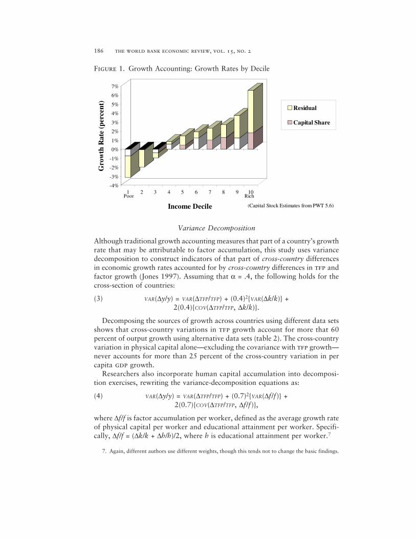
Aggregate growth accounting results are illustrated in figure 1 using data fromPWT 5.6 for 1980–92. Countries are grouped by decile based on output per capitagrowth, from the slowest growing (group 1) to the fastest. Capital growth gen-erally accounts for less than half of output growth, and the share of growth ac-counted for by tfp growth is frequently larger in the faster growing countries.There are large differences across countries in the relationship between capitalaccumulation and growth. For example, Costa Rica, Ecuador, Peru, and Syriaall saw real per capita gdp fall by more than 1 percent a year, while real percapita capital stocks grew by more than 1 percent a year and educational attain-ment was rising. Clearly, these factor injections were not being used productiv-ity. Albeit unrepresentative, these cases illustrate the shortcoming of focusingtoo heavily on factor accumulation.6
Incorporating estimates of human capital accumulation into these aggregategrowth accounting exercises does not materially alter the findings. In the aver-age country, tfp growth still accounts for more than half of growth in outputper worker. Moreover, the data suggest a weak—and sometimes inverse—rela-tionship between improvements in educational attainment of the labor force andgrowth of output per worker growth. Benhabib and Spiegel (1994) and Pritchett(2001), using cross-country data on economic growth rates, show that increasesin human capital resulting from improvements in educational attainment havenot positively affected the growth in output per worker (perhaps because of amismatch between education and the skills needed for activities that generatesocial returns).
There is disagreement, however. Krueger and Lindahl (1999) argue that mea-surement error accounts for the failure to find a relationship between growthper capita and human capital accumulation. Hanushek and Kimko (2000) findthat the quality of education is strongly linked with economic growth. Klenow(1998) demonstrates that models that highlight the role of ideas and productiv-ity growth do a much better job of matching the data than models that focus onthe accumulation of human capital. More work is needed on the relationshipbetween education and economic development.
6. It may be that the conventional measure of investment effort is a cost-based measure that doesnot translate necessarily into increasing the value of the capital stock. Pritchett (1999) makes this point,especially—but not only—with regard to public investment.
186 the world bank economic review, vol. 15, no. 2
Variance Decomposition
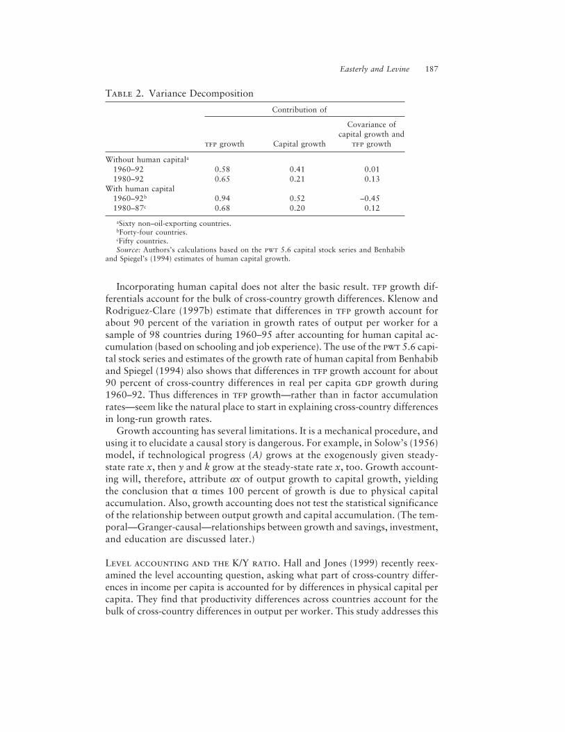
Although traditional growth accounting measures that part of a country’s growthrate that may be attributable to factor accumulation, this study uses variancedecomposition to construct indicators of that part of cross-country differencesin economic growth rates accounted for by cross-country differences in tfp andfactor growth (Jones 1997). Assuming that α = .4, the following holds for thecross-section of countries:
(3) VAR(Dy/y) = VAR(DTFP/TFP) + (0.4)2{VAR(Dk/k)} +2(0.4){COV(DTFP/TFP, Dk/k)}.
Decomposing the sources of growth across countries using different data setsshows that cross-country variations in tfp growth account for more that 60percent of output growth using alternative data sets (table 2). The cross-countryvariation in physical capital alone—excluding the covariance with tfp growth—never accounts for more than 25 percent of the cross-country variation in percapita gdp growth.
Researchers also incorporate human capital accumulation into decomposi-tion exercises, rewriting the variance-decomposition equations as:
(4) VAR(Dy/y) = VAR(DTFP/TFP) + (0.7)2{VAR(Df/f)} +2(0.7){COV(DTFP/TFP, Df/f )},
where Df/f is factor accumulation per worker, defined as the average growth rateof physical capital per worker and educational attainment per worker. Specifi-cally, Df/f = (Dk/k + Dh/h)/2, where h is educational attainment per worker.7
Figure 1. Growth Accounting: Growth Rates by Decile
7. Again, different authors use different weights, though this tends not to change the basic findings.
-4%
-3%
-2%
-1%
0%
1%
2%
3%
4%
5%
6%
7%
Gro
wth
Rat
e (p
erce
nt)
1 2 3 4 5 6 7 8 9 10
Income Decile
Residual
Capital Share
Poor Rich
(Capital Stock Estimates from PWT 5.6)
Easterly and Levine 187
Incorporating human capital does not alter the basic result. tfp growth dif-ferentials account for the bulk of cross-country growth differences. Klenow andRodriguez-Clare (1997b) estimate that differences in tfp growth account forabout 90 percent of the variation in growth rates of output per worker for asample of 98 countries during 1960–95 after accounting for human capital ac-cumulation (based on schooling and job experience). The use of the pwt 5.6 capi-tal stock series and estimates of the growth rate of human capital from Benhabiband Spiegel (1994) also shows that differences in tfp growth account for about90 percent of cross-country differences in real per capita gdp growth during1960–92. Thus differences in tfp growth—rather than in factor accumulationrates—seem like the natural place to start in explaining cross-country differencesin long-run growth rates.
Growth accounting has several limitations. It is a mechanical procedure, andusing it to elucidate a causal story is dangerous. For example, in Solow’s (1956)model, if technological progress (A) grows at the exogenously given steady-state rate x, then y and k grow at the steady-state rate x, too. Growth account-ing will, therefore, attribute ax of output growth to capital growth, yieldingthe conclusion that a times 100 percent of growth is due to physical capitalaccumulation. Also, growth accounting does not test the statistical significanceof the relationship between output growth and capital accumulation. (The tem-poral—Granger-causal—relationships between growth and savings, investment,and education are discussed later.)
Level accounting and the K/Y ratio. Hall and Jones (1999) recently reex-amined the level accounting question, asking what part of cross-country differ-ences in income per capita is accounted for by differences in physical capital percapita. They find that productivity differences across countries account for thebulk of cross-country differences in output per worker. This study addresses this
Table 2. Variance Decomposition
Contribution of
Covariance ofcapital growth and
tfp growth Capital growth tfp growth
Without human capitala
1960–92 0.58 0.41 0.011980–92 0.65 0.21 0.13
With human capital1960–92b 0.94 0.52 –0.451980–87c 0.68 0.20 0.12
aSixty non–oil-exporting countries.bForty-four countries.cFifty countries.Source: Authors’s calculations based on the pwt 5.6 capital stock series and Benhabib
and Spiegel’s (1994) estimates of human capital growth.
188 the world bank economic review, vol. 15, no. 2
question using the traditional Denison (1962) approach and a modified Mankiw,Romer, and Weil (1992) approach.
To conduct Denison-level accounting, take the ratio of two national incomesof output per person from equation 1:
(5) [yi / yi] = [Ai / Aj][ki / kj]a[ni / nj]1–a.
Given data on the factors of production, cross-country differences in tfp can bemeasured by:
(6) [Ai / Aj] = [yi / yj]/{[ki / kj]a[ni / nj]1–a}.
The fraction of differences in national output levels due to capital equals theratio, φki.
(7) φki = alog(ki / kj) / log(yi / yj).
Equation 7 can be rewritten as:
(8) φki = a + alog(ki / kj) / log(yi / yj),
because log(ki/kj) = log(κi/κj) – log(yyi/yj), letting κ=k/y. This allows measurementof the contribution of capital due to capital share (a) and that due to differencesin the capital-output ratios. If capital-output ratios are constant across coun-tries i and j, then the contribution of capital due to differences in output per capitain countries i and j simply equals a.
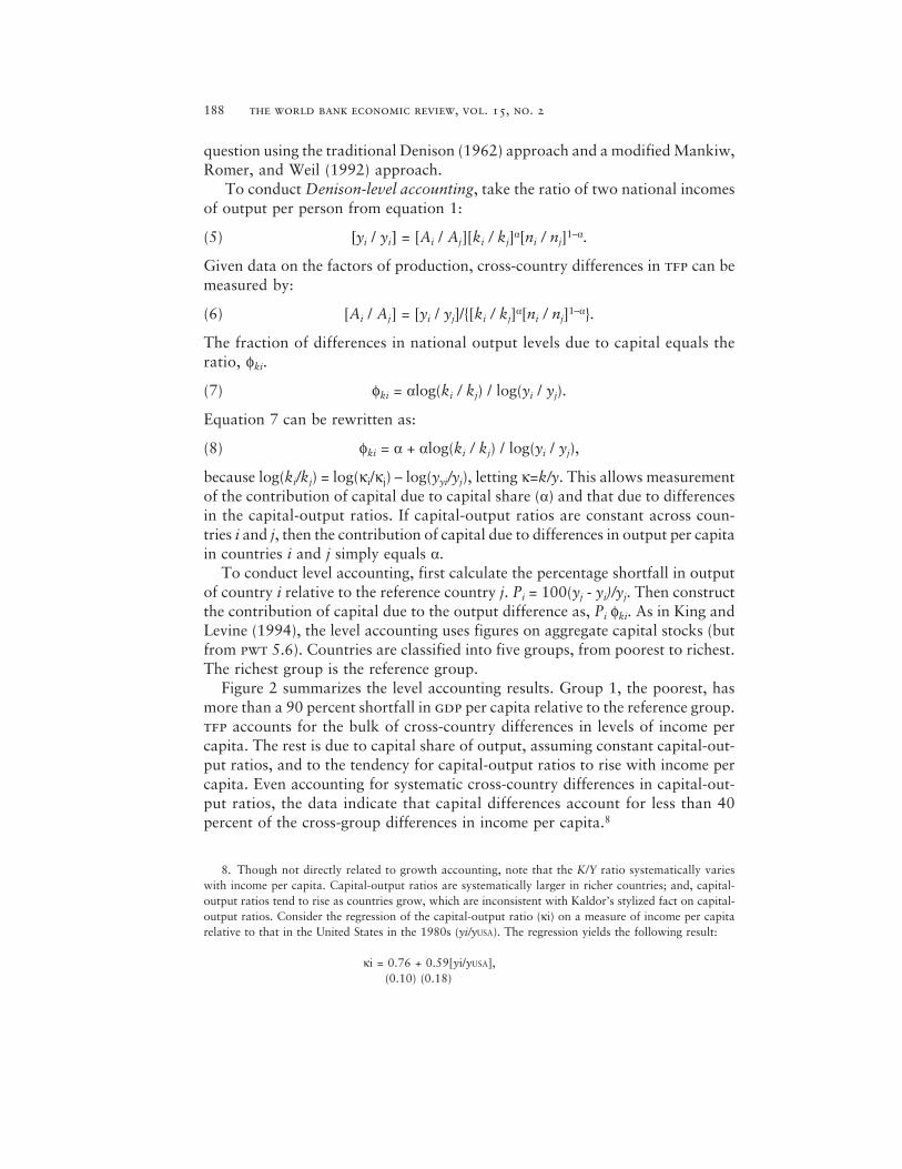
To conduct level accounting, first calculate the percentage shortfall in outputof country i relative to the reference country j. Pi = 100(yj - yi)/yj. Then constructthe contribution of capital due to the output difference as, Pi φki. As in King andLevine (1994), the level accounting uses figures on aggregate capital stocks (butfrom pwt 5.6). Countries are classified into five groups, from poorest to richest.The richest group is the reference group.
Figure 2 summarizes the level accounting results. Group 1, the poorest, hasmore than a 90 percent shortfall in gdp per capita relative to the reference group.tfp accounts for the bulk of cross-country differences in levels of income percapita. The rest is due to capital share of output, assuming constant capital-out-put ratios, and to the tendency for capital-output ratios to rise with income percapita. Even accounting for systematic cross-country differences in capital-out-put ratios, the data indicate that capital differences account for less than 40percent of the cross-group differences in income per capita.8
8. Though not directly related to growth accounting, note that the K/Y ratio systematically varieswith income per capita. Capital-output ratios are systematically larger in richer countries; and, capital-output ratios tend to rise as countries grow, which are inconsistent with Kaldor’s stylized fact on capital-output ratios. Consider the regression of the capital-output ratio (κi) on a measure of income per capitarelative to that in the United States in the 1980s (yi/yUSA). The regression yields the following result:
κi = 0.76 + 0.59[yi/yUSA],(0.10) (0.18)
Easterly and Levine 189
Mankiw, Romer, and Weil (mrw) level accounting. A second approach tolevel accounting is suggested by Mankiw, Romer, and Weil (1992), who arguethat the Solow model does a good job of accounting for cross-country differ-ences in the level of income per capita. In the steady-state of the Solow model,output per person is given by:
(9) Y/L = A [s/(x+δ+n)] α/(1-α),
where Y/L is output per person, A is the level of labor-augmenting productivity,s is the ratio of investment to gdp, x is the rate of labor-augmenting productiv-ity growth, d is depreciation, n is population growth, and a is the share of capi-tal income in gdp. A 2 percent productivity growth rate and a 7 percent depre-ciation rate are assumed. Logs are taken of both sides, and the log of output perperson is regressed on a constant (ln A) and on the log of the second multiplica-tive term in equation 9:
Figure 2. Development Accounting by Income Quintiles(57 Non-Oil-Exporting Countries)
where ki is the capital-output ratio in country i, standard errors are in parentheses, and the regressionincludes 57 non-oil-exporting countries. There is a strong positive relationship between output per personrelative to the United States and the K/Y ratio. Also, figure 3 shows that the K/Y ratio tends to rise infast growing countries. Here, the average value of K/Y ratios are plotted year by year for countries withper capita growth rates higher than 3.5 percent a year over the period 1960–92. The K/Y ratio risesrapidly over this fast growth period. Though these differences might be due to transitional dynamics,past works suggests that physical capital accumulation along the transition path is unlikely to explainfully level and growth differences (King and Rebelo 1993).
Note: Data cover 57 non-oil-exporting countries.Source: Authors’ calculations based on Penn World Table 5.6 for capital stock estimates.
0
10
20
30
40
50
60
70
80
90
100
Shor
tfal
l Rel
ativ
e to
Fif
thQ
uint
ile
1 2 3 4
Quintile
Residual
Differences inK/Y
Capital Share

190 the world bank economic review, vol. 15, no. 2
(10) ln(Y/L) = ln A + a/(1-a) [ln s — ln(x+δ+n)].
This second term will be called MRW.The mrw approach is then extended by allowing A to differ across regions,
oil-producing and non–oil-producing countries, and oecd and non-oecd coun-tries. (The regions are all-inclusive; the OECD and OIL dummy variables measureshifts relative to their respective regions.)
Though there is a significant correlation of income with the mrw investmentterm (consistent with the Solow model), the results in table 3 refute the originalmrw idea that productivity levels are the same across countries. South Asia andSub-Saharan Africa have significantly lower productivity than other regions (in-come differences that are not explained by the mrw term). The oecd has higherproductivity than the rest of the world by a factor of 3 (e1.087). Once the produc-tivity level is allowed to vary, the coefficient on mrw implies a capital share of.31—which is in line with most estimates from national income accounting.
Mankiw, Romer, and Weil report that they are even more successful at ex-plaining cross-country income differences when they include a measure of humancapital investment, which they define as [ln sh — ln(x + δ + n)]. They define theflow of investment in human capital sh
as the secondary enrollment ratio timesthe proportion of the labor force of secondary school age. Klenow and Rodriguez-Clare (1997b) and Romer (1995) criticize this measure as overestimating thecross-country variation in human capital by ignoring primary enrollment, whichvaries much less across countries than secondary enrollment. The results for this
Table 3. mrw Least Squares Regression with Regional, Oil, and oecdDummy Variables
Variable Coefficient Standard error t-statistic Probability
oecd 1.087817 0.107084 10.15857 0.0000East Asia 7.559995 0.176696 42.78525 0.0000South Asia 7.065895 0.139239 50.74634 0.0000Sub-Saharan Africa 6.946945 0.090968 76.36658 0.0000Western Hemisphere 7.838313 0.102363 76.57349 0.0000Middle East and North Africa 7.777138 0.143632 54.14642 0.0000Europe 7.717543 0.133190 57.94384 0.0000OIL 0.691058 0.157605 4.384760 0.0000MRW 0.442301 0.096847 4.567031 0.0000
R2 0.752210 Mean dependent variable 7.79Adjusted R2 0.738969 Standard error of dependent 0.994
variableStandard error of regression 0.508076 Akaike information criterion 1.539Sum of squared residual 33.81651 Schwarz criterion 1.708Log likelihood –98.99247 F-statistic 56.810
Probability (F-statistic) 0.000
Note: Average log income per capita in 1960–95 is the dependent variable. Number of observations= 139. Standard errors and covariance are White heteroskedasticity-consistent.
Source: Authors’ calculations based on World Bank data.
Easterly and Levine 191
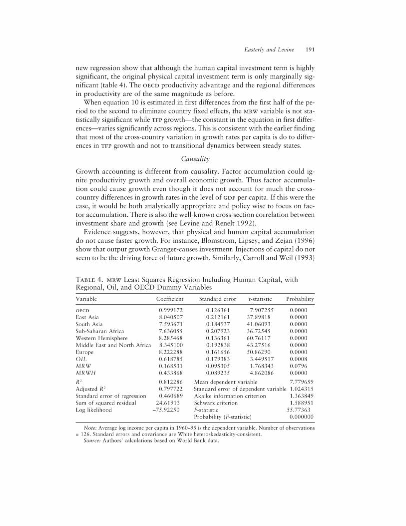
new regression show that although the human capital investment term is highlysignificant, the original physical capital investment term is only marginally sig-nificant (table 4). The oecd productivity advantage and the regional differencesin productivity are of the same magnitude as before.
When equation 10 is estimated in first differences from the first half of the pe-riod to the second to eliminate country fixed effects, the mrw variable is not sta-tistically significant while tfp growth—the constant in the equation in first differ-ences—varies significantly across regions. This is consistent with the earlier findingthat most of the cross-country variation in growth rates per capita is do to differ-ences in tfp growth and not to transitional dynamics between steady states.
Causality
Growth accounting is different from causality. Factor accumulation could ig-nite productivity growth and overall economic growth. Thus factor accumula-tion could cause growth even though it does not account for much the cross-country differences in growth rates in the level of gdp per capita. If this were thecase, it would be both analytically appropriate and policy wise to focus on fac-tor accumulation. There is also the well-known cross-section correlation betweeninvestment share and growth (see Levine and Renelt 1992).
Evidence suggests, however, that physical and human capital accumulationdo not cause faster growth. For instance, Blomstrom, Lipsey, and Zejan (1996)show that output growth Granger-causes investment. Injections of capital do notseem to be the driving force of future growth. Similarly, Carroll and Weil (1993)
Table 4. mrw Least Squares Regression Including Human Capital, withRegional, Oil, and OECD Dummy Variables
Variable Coefficient Standard error t-statistic Probability
oecd 0.999172 0.126361 7.907255 0.0000East Asia 8.040507 0.212161 37.89818 0.0000South Asia 7.593671 0.184937 41.06093 0.0000Sub-Saharan Africa 7.636055 0.207923 36.72545 0.0000Western Hemisphere 8.285468 0.136361 60.76117 0.0000Middle East and North Africa 8.345100 0.192838 43.27516 0.0000Europe 8.222288 0.161656 50.86290 0.0000OIL 0.618785 0.179383 3.449517 0.0008MRW 0.168531 0.095305 1.768343 0.0796MRWH 0.433868 0.089235 4.862086 0.0000
R2 0.812286 Mean dependent variable 7.779659Adjusted R2 0.797722 Standard error of dependent variable 1.024315Standard error of regression 0.460689 Akaike information criterion 1.363849Sum of squared residual 24.61913 Schwarz criterion 1.588951Log likelihood –75.92250 F-statistic 55.77363
Probability (F-statistic) 0.000000
Note: Average log income per capita in 1960–95 is the dependent variable. Number of observations= 126. Standard errors and covariance are White heteroskedasticity-consistent.
Source: Authors’ calculations based on World Bank data.

192 the world bank economic review, vol. 15, no. 2
show that causality tends to run from output growth to savings, not the otherway around. Evidence on human capital tells a similar story. Bils and Klenow(1996) argue that the direction of causality runs from growth to human capital,not from human capital to growth. Thus in terms of both physical and humancapital, the data do not provide strong support for the contention that factoraccumulation ignites faster growth in output per worker.
Summary
Although there are important exceptions, as Young (1995) makes clear, “some-thing else” besides factor inputs accounts for the bulk of cross-country differ-ences in income per capita and growth rates. Furthermore, although growth ac-counting does not show causality, research suggests that increases in factoraccumulation do not ignite faster output growth in the future. While more workis needed, the evidence does not suggest that causality runs from physical orhuman capital accumulation to economic growth in the broad cross-section ofcountries. Finally, measurement error may reduce confidence in growth and levelaccounting. However, the residual is large in both level and growth accounting.Also, level and growth accounting for the 1950s and 1960s produce similar es-timates as those for the 1990s. This implies that measurement error would haveto have two systematic components. Both the growth rate of measurement errorand the level component of measurement error would have to be positive andlarge in rich, fast-growing countries. Measurement problems may play a role,but a considerable body of evidence suggests that something else—tfp—besidesfactor accumulation is critical for understanding cross-country differences in thelevel and growth of gdp per capita.
In giving theoretical content to this residual, Grossman and Helpman (1991),Romer (1990) and Aghion and Howitt (1998) focus on technology, on betterinstructions for combining raw materials into useful products and services. Romer(1986), Lucas (1988), and others focus on externalities, including spillovers,economies of scale, and various complementarities in explaining the large roleplayed by tfp.9 Harberger (1998) views tfp as real cost reductions and urgeseconomists not to focus on one underlying cause of tfp because several factorsmay produce real costs reductions in different sectors of the economy at differ-ent times.10 This is consistent with industry studies that reveal considerable cross-sector variation in tfp growth (Kendrick and Grossman 1980). Prescott (1998)also focuses on technology. He suggests that cross-country differences in resis-tance to the adoption of better technologies—arising from politics and policies—help explain cross-country differences in tfp (see Holmes and Schmitz 1995;Parente 1994; Parente and Prescott 1996; and Shleifer and Vishny 1993). It would
9. Yet, Burnside (1996) presents evidence suggesting that physical capital externalities are relativelyunimportant. Klenow (1998) presents evidence that is consistent with technological change-based modelof growth.
10. Costello (1993) shows that TFP has a strong country component and is not specific to particularindustries.

Easterly and Levine 193
be useful in designing models and policies to determine empirically the relativeimportance of each of these conceptions of tfp.
III. Stylized Fact 2. Divergence, Not Convergence,Is the Big Story
Over the very long run, there has been “divergence, big time,” in the words ofPritchett (1997). The richest countries in 1820 subsequently grew faster than thepoorest countries in 1820. The ratio of richest to poorest went from 6 to 1 in 1820to 70 to 1 in 1992 (figure 3). Prior to the Industrial Revolution (1700–50), thedifference between the richest and poorest countries was probably only about 2to 1 (Bairoch 1993, pp. 102–6). Thus, the big story over the past 200–300 yearsis one of massive divergence in the levels of income per capita between the richand the poor.11
The poor are not getting poorer, but the rich are getting richer a lot faster thanthe poor. Absolute divergence has continued over the past 30 years, though not asdramatically as in earlier periods (see table 5). And while China and India—countries with very large populations—have performed well recently, growth hasdiverged significantly even using recent data.12
Moreover, the data presented in table 5 understate absolute divergence over1960–92 because data were lacking for many low- and middle-income countriesfor the 1990s but not for any high-income countries. This imparts a bias towardconvergence in the data similar to that pointed out by De Long (1988) regard-ing Baumol’s (1986) finding of convergence among industrial countries. Whenthe countries that are rich at the end are overrepresented in the sample, the sampleis biased toward convergence. The growth rates of the lower three-fifths of thesample would be even lower if data were available for some of the poorly per-forming low- and middle-income economies in the 1990s.
Within the postwar period, this tendency toward divergence has become morepronounced with time. Easterly (2001) found that the bottom half of countriesordered by per capita income in 1980 registered zero per capita growth over1980–98, while the top half continued to register positive growth. The reasonwas not a divergence in policies; policies in poor countries were converging to-ward those of rich countries over 1980–98.
Although many cross-economy data sets exhibit conditional convergence (Barroand Sala-i-Martin 1992), it is difficult to look at the growing differences betweenthe rich and poor and not focus on divergence. Conditional convergence findingshold only after conditioning on an important mechanism for divergence—spillovers
11. See Lucas (1998) for an extensive discussion of this divergence, which he interprets as reflectingdifferent takeoff times for various economies, and which he predicts will decrease as new countriestake off.
12. The usual finding that initial income and growth are uncorrelated relied on data that went through1981 or 1985, using a linear regression of growth on initial income. The use of more recent data (through1992) and the analysis of quintiles account for this finding of absolute divergence.

194 the world bank economic review, vol. 15, no. 2
from the initial level of knowledge (for which conditional convergence regressionsmay be controlling with initial level of schooling). Conditional convergence alsocould follow mechanically from mean reversion (Quah 1993). Because most growthmodels are closed economy models, it is worth looking at what happens to con-vergence in closed economies. Kremer (1993) and Ades and Glaeser (1999) havefound absolute divergence in the majority of closed developing economies, sug-gesting an “extent of the market” effect on growth in closed economies.
These findings on divergence should be seen within the context of other styl-ized facts. Romer (1986) shows that the growth rates of the riches countries have
Note: Order in 1820 from richest (top) to poorest (bottom).Source: Maddison 1995.
Figure 3. Growth Rates Diverge between Rich and Poor: 1820–1992
1820 1992
Rat
io t
o "s
ubsi
sten
ce"
inco
me,
log
base
2 s
cale
UK
Netherlands
Australia
Austria
Belgium
USA
Denmark
France
Sweden
Germany
Italy
Spain
Norway
Ireland
Canada
Czechoslovakia
Mexico
Finland
USSR
Japan
Brazil
Indonesia
Nigeria
Bangladesh
India
Pakistan
China
Egypt
Ghana
Tanzania
Burma
Zaire
Ethiopia
Lesotho
Togo
Malawi
2
4
8
16
32
64
1
(top) to poorest (bottom)
Easterly and Levine 195
not slowed over the last century. King and Rebelo (1993) show that returns tocapital in the United States have not been falling over the last century. Together,these observations do not naturally suggest a model that emphasizes capital ac-cumulation and that has diminishing returns to factors, some fixed factor ofproduction, and constant returns to scale. Neither do they provide unequivocalsupport for any particular conception of what best explains the something elsebehind these stylized facts.
IV. Stylized Fact 3. Growth Is Not Persistent,but Factor Accumulation Is
Growth is remarkably unstable over time. The correlation of per capita growthin 1977–92 with per capita growth in 1960–76 across 135 countries is only .08.13
This low persistence is not just a characteristic of the postwar era. For the 25countries for which there are data (Maddison 1995), the correlation between1820–70 and 1870–1929 is only .097.
In contrast, the cross-period correlation of growth in capital per capita is 0.41.For models that postulate a linear relationship between growth and the share ofinvestment in gdp (using investment share in gdp as an alternative measure ofcapital accumulation), the mismatch in persistence is even worse.14 The correla-tion of investment share in gdp in 1977–92 with investment share in 1960–76 is.85. Nor do models that postulate growth per capita as a function of humancapital accumulation do better. The correlation across 1960–76 and 1977–92for primary enrollment is .82, while the cross-period correlation for secondaryenrollment is .91. This suggests that much of the large variation of growth over
13. Data on per capita growth are from the pwt 5.6. The low persistence of growth rates, and thehigh persistence of investment and education, was previously noted in Easterly and others (1993).
14. Models supposing a linear relationship between growth and investment have a long history ineconomics. See Easterly (1999b) for a review of the Harrod-Domar tradition that continues down tothe present. For a new growth theory justification of this relationship, see McGrattan (1998).
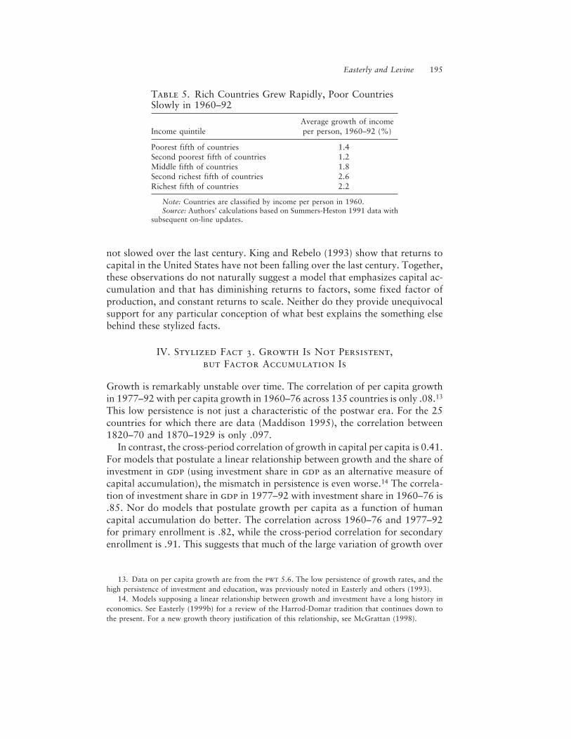
Table 5. Rich Countries Grew Rapidly, Poor CountriesSlowly in 1960–92
Average growth of incomeIncome quintile per person, 1960–92 (%)
Poorest fifth of countries 1.4Second poorest fifth of countries 1.2Middle fifth of countries 1.8Second richest fifth of countries 2.6Richest fifth of countries 2.2
Note: Countries are classified by income per person in 1960.Source: Authors’ calculations based on Summers-Heston 1991 data with
subsequent on-line updates.

196 the world bank economic review, vol. 15, no. 2
time is not explained by the much smaller variation in physical and human capi-tal accumulation.
Takeoff into Steady-State Growth Is Rare
The typical model of growth, in both the old and new growth literatures, fea-tures a steady-state growth rate. Historically, this was probably inspired by theU.S. experience of remarkably steady growth of about 2 percent per capita overnearly two centuries (Jones 1995a, 1995b; Rebelo and Stokey 1995).
Because all countries must have had prior histories of stagnation, another char-acterization of the typical growth path is the “takeoff into self-sustained growth”(the phrase is from Rostow 1960; more recent theoretical modeling of takeoffincludes Baldwin 1998, Krugman and Venables 1995, Jones 1999, Lucas 1998,and Hansen and Prescott 1998). The prevailing image is a smooth accelerationfrom stagnation into steady-state growth. Developing countries are supposed tohave taken off beginning in the 1960s, when their growth was rapid and exceededexpectations.
Experience did not bear out the idea of steady growth beginning in the 1960s.Many countries experienced booms and crashes (Pritchett 2000, Rodrik 1998).Even when ten-year average growth rates are used, which should be long enoughto iron out cyclical swings, the cross-section standard deviation is about 2.5percentage points and the variation over time swamps the cross-section varia-tion. In 48 of 119 countries with 20 years or more of data over 1960–97, abreakpoint can be found in which the subsequent decade’s per capita growthis more than 5 percentage points—two cross-section standard deviations—above or below the previous decade’s growth.15All of the countries with growthbooms or crashes were developing countries, except for Greece and Portugal.Figure 4 illustrates the rollercoaster ride of Côte d’Ivoire, Guyana, Jamaica,and Nigeria.
Stable growth may be a better description of industrial than developing coun-tries. Of 88 industrial and developing countries with complete data for 1960–97, only 12 had growth above 2 percent per capita in every decade. Half were inEast Asia.
Variance Decomposition over Time
This supposition of unstable growth is further confirmed by variance decom-position exercises, with decomposition over time rather than across countries.In conjunction with the cross-country variance decomposition presented above,this analysis represents a full exploration of the panel data on growth and itsfactors.
A panel of seven five-year time periods was constructed for each country forper capita growth and growth in physical capital per capita. Country means are
15. Thirty-seven countries had a growth drop of 5 percentage points or more, 19 countries of5 percentage points or more, and 8 countries were included in both groups.

Easterly and Levine 197
then subtracted and the variance is analyzed using the same formula as before(see equation 3). For the same sample of countries, tfp accounts for 86 percentof the intertemporal variation in overall growth and 61 percent of the cross-sectional variation. Thus, growth is much more unstable over time than physi-cal capital growth.
Besides emphasizing the importance of tfp in explaining long-run developmentpatterns, the findings that growth is not persistent and that growth patterns arevery different across countries complicate the challenge for economic theorists.
-0.2
-0.1
0
0.1
0.2
0.3
0.4
0.5
0.6
0.7
0.8
1960 1963 1966 1969 1972 1975 1978 1981 1984 1987 1990 1993 1996
Cum
ulat
ive
log
per
capi
ta g
row
th s
ince
196
0
Cote d'Ivoire
Jamaica
Nigeria
Guyana
Figure 4. Examples of Variable Per Capita Income over Time: 1960–96
Source: World Bank data.

198 the world bank economic review, vol. 15, no. 2
Existing models miss important development experiences. Some countries growsteadily (the United States). Some grow steadily and then stop for long periods(Argentina). Some do not grow for long periods and then suddenly take off (Re-public of Korea, Thailand). Others have never grown (Somalia). Accounting forthese very different growth experiences will be very difficult with sole reliance oneither steady-state models or standard multiple-equilibria models. Different mod-els may be needed for different patterns of growth across countries. Steady-statemodels fit the U.S. type experience. Multiple equilibria models are a better fit forunstable growth cases because countries’ long-run fundamentals are stable.16
V. Stylized Fact 4. When It Rains, It Pours:All Factors Flow in the Same Direction
This section presents new information on the concentration of economicactivity, using cross-country data, data from counties in the United States,information on developing countries, and data on international flows of capi-tal, labor, and human capital. This concentration has a fractal-like quality.It recurs at all levels of analysis, from the global to the urban. It suggests thatsome regions have “something” that attracts all factors of production, whereasothers do not.
Better policies (legal systems, property rights, political stability, public edu-cation, infrastructure, taxes, regulations, macroeconomic stability) in one areathan in another could explain these factor flows. But such policies are national;they cannot explain findings of within-country concentration (discussed below).Externalities may lead to factor congregation. Critically, policy differences, orexternalities, or differences in something else do not have to be large. Small dif-ferences can have dramatic long-run implications. So, although no specific ex-planation is offered, the results of this analysis suggest a need for more work oneconomic geography as a vehicle for understanding economic growth.
Concentration
An obvious observation at the global level is that high income is concentratedamong a small number of countries (see map 1). The top 20 countries have only15 percent of world population but produce 50 percent of world gdp. The poorest
16. The nonpersistence of growth rates does not inherently contradict the stylized fact of diver-gence or the stylized fact that national policies influence long-run growth rates. While policies are per-sistent and significantly associated with long-run growth (which is not persistent), the R2 of the growthregression is generally smaller than 0.50. Thus, something else (besides national policies) is very impor-tant for explaining cross-country differences in long-run growth rates. In terms of divergence, the styl-ized fact of the nonpersistence of growth rates emphasizes that growth follows very different paths acrosscountries and that there is a high degree of volatility. Nevertheless, there are countries that have achievedcomparatively greater success over the long run. While France, Germany, and the United Kingdom haveexperienced growth fluctuations, they have enjoyed a steeper—and less volatile—growth path thanArgentina and Venezuela, for example, whose growth paths have not only been more volatile but ex-hibited dramatic changes in trends.

Easterly and Levine 199
half of the world’s population accounts for only 14 percent of its gdp.17 Theseconcentrations of wealth and poverty have an ethnic and geographic dimen-sion: 18 of the top 20 countries are in Western Europe or were settled primarilyby Western Europeans; 17 of the poorest 20 countries are in tropical Africa. Therichest country in 1985 (the United States) had an income 55 times that of thepoorest country (Ethiopia). When inequality within countries is considered, in-ternational income differences are even starker. The income of the richest quintilein the United States was 528 times that of the poorest quintile in Guinea-Bissau.
Income is highly concentrated by area as well, as shown by data on gdp persquare kilometer. The densest 10 percent of world land area accounts for 54percent of global gdp; the least dense for only 11 percent.18
These calculations understate the degree of concentration because they assumethat income is evenly spread among people and land area within countries. Amore detailed look within countries also shows high concentrations of wealthand poverty.
Map 1. The Rich and the Poor
The countries in black contain 15 percent of world population but produce 50 percent of world gdp.The countries in gray contain 50 percent of world population but produce 14 percent of world gdp.
17. These calculations omit the oil-exporting countries, in which GDP is not properly measured be-cause all of oil extraction is treated as current income rather than asset depletion.
18. An alternative explanation would be that some land areas, accounting for a small share of theearth’s surface, have a large productivity advantage. Mellinger, Sachs, and Gallup (1999) argue thattemperate coastal zones have a large productivity advantage. If this were true, economic activity wouldbe distributed fairly evenly along temperate coastal zones (adjusting for any small intrinsic differencesamong such zones). However, even along temperate coastal zones, casual observations would suggesthigh bunching of activity.

200 the world bank economic review, vol. 15, no. 2
Consider the United States. Data on gdp per square mile for 3,141 countiesshow that counties accounting for only 2 percent of the land produce 50 percentof gdp, while the least dense counties that account for 50 percent of the landproduce only 2 percent of gdp (map 2). Nor is this finding a consequence merelyof the large unsettled areas of the West and Alaska. The same calculation forland east of the Mississippi River yields similarly extreme concentration: 50percent of gdp is produced on 4 percent of the land. The densest county is NewYork, New York, with a gdp per square mile of $1.5 billion. This is about 55,000times more than the least dense county east of the Mississippi ($27,000 per squaremile in Keweenaw, Michigan). Even this understates the degree of concentra-tion because even the most casual empiricism will detect rich and poor areaswithin a given county (New York county contains Harlem as well as Wall Street).
The concentration of counties accounting for half of U.S. gdp is explained bythe fact that these are metropolitan counties and most economic activity takesplace in densely populated metropolitan areas. Metropolitan counties are $3,300richer per person than rural counties (the difference is statistically significant,with a t-statistic of 29). More generally, there is a strong correlation betweenper capita income of U.S. counties and their population density (correlationcoefficient of .48 for the log of both concepts, with a t-statistic of 30 on the bi-variate association). But concentration is high even within metropolitan coun-ties: 50 percent of metropolitan gdp is produced in counties accounting for only6 percent of metropolitan land area.19
There are also regional income differences between metropolitan areas.Metropolitan areas in the Boston–Washington corridor have a per capita in-
19. Metropolitan counties are those that belong to a pmsa or msa in the census classification ofcounties.
Map 2. Densely Populated U.S. Counties
Counties shown in black take up 2 percent of U.S. land area but account for half of U.S. gdp.

Easterly and Levine 201
come $5,874 higher on average than other metropolitan areas. This is a hugedifference: It is equal to 2.4 standard deviations in the metropolitan area sample.Although there may be differences in the cost of living, they are unlikely to beso large as to explain this difference. (The rent component of the cost of livingmay reflect the productivity or the amenity advantages of the area—it seemsunlikely that amenities are different enough among areas to explain thesedifferences.)
There are other possible explanations of geographic concentration, such asinherent geographic advantages. Like Mellinger, Sachs, and Gallup (1999),Rappaport and Sachs (1999) argue that spatial concentration of activity in theUnited States has much to do with access to the coast. However, casual observa-tion suggests high concentration even within coastal areas (there are sections alongthe Boston–Washington corridor with no radio reception). Some studies suggestthat high transport costs and low congestion costs could also play a role (Krugman1991, 1995, 1998; Fujita, Krugman, and Venables 1999). However, these stud-ies also point to locations of particular industries (the Silicon Valley phenom-enon) as evidence of other types of geographic spillover, including technologyspillovers and specialized producer services with high fixed costs. And the highrents in downtown metropolitan areas suggest that congestion costs are signifi-cant. As Lucas (1988, p. 39) says, “What can people be paying Manhattan ordowntown Chicago rents for, if not for being near other people?”
Poor Areas
Like wealth, poverty is also concentrated. In the United States, poverty is region-ally concentrated. These concentrations have an ethnic dimension as well (seemap 3). Four ethnogeographic clusters of counties have poverty rates above 35percent:
• Counties in the West with large proportions (> 35 percent) of Native Americans.• Counties along the Mexican border with large proportions (> 35 percent)
of Hispanics.• Counties along the lower Mississippi River in Arkansas, Mississippi, and
Louisiana and in the “black belt” of Alabama, all of which have large pro-portions of blacks (> 35 percent).
• Virtually all-white counties in the mountains of eastern Kentucky.
The county data did not pick up the well-known phenomenon of inner-citypoverty, mainly among blacks, because counties that include inner cities alsoinclude rich suburbs. (An isolated example of an all-black city is East St. Louis,Illinois, which is 98 percent black and has a poverty rate of 44 percent.) Of course,poverty is concentrated in the inner city as well. An inner city zip code in Wash-ington, D.C., College Heights in Anacostia, has only one-fifth of the income ofa rich zip code in Bethesda, Maryland. This has an ethnic dimension again be-cause College Heights is 96 percent black and the rich zip code in Bethesda is96 percent white. The Washington, D.C., metropolitan area as a whole shows

202 the world bank economic review, vol. 15, no. 2
the striking East–West divide between poor and rich zip codes, which againroughly corresponds to the black–white ethnic divide (see map 4).20
Borjas (1995, 1999) suggests that strong neighborhood and ethnic externali-ties may help explain poverty and ethnic clusters within cities. The 1990 censustracts with the highest shares of blacks have 50 percent of the black populationbut only 1 percent of the white population.21 Although this segregation by raceand class could simply reflect the preferences of rich white people to live next toeach other, economists usually prefer to offer economic motivations rather thanexogenous preferences as explanations of economic phenomena. Benabou (1993,1996) stresses the endogenous sorting between rich and poor, so the rich cantake advantage of such externalities as locally funded schools.
Poverty areas exist within many countries: northeast Brazil, southern Italy,Chiapas in Mexico, Balochistan in Pakistan, and the Atlantic Provinces in Canada.Researchers have found that externalities explain part of these poverty clusters.Bouillon, Legovini, and Lustig (1999) find a negative Chiapas effect in Mexicanhousehold income data, an effect that has worsened over time. Households in thepoor region of Tangail-Jamalpur in Bangladesh earned less than households withsimilar characteristics in the better-off region of Dhaka (Ravallion and Wodon1998). Ravallion and Jalan (1996) and Jalan and Ravallion (1997) likewise foundthat households in poor counties in southwest China earned less than householdswith identical human capital and other characteristics in rich Guangdong Prov-ince. Rauch (1993) found that individuals with identical characteristics earn lessin low human capital cities in the United States than in high human capital cities.
20. Brookings Institution (1999) notes that this East–West geographic divide of the Washington,D.C., area shows up in many socioeconomic variables (poverty rates, free and reduced price schoollunches, road spending).
21. From the Urban Institute’s Underclass Database, which contains data on white, black, and“other” population numbers for 43,052 census tracts in the United States.
Map 3. Poverty Traps in the U.S. County Data
Counties in black have more than 35 percent poverty rate.

Easterly and Levine 203
Ethnic and Related Differentials
Some theories stress in-group externalities (Borjas 1992, 1995, 1999; Benabou1993, 1996). Poverty and riches are also concentrated in certain ethnic groups.Exogenous savings preferences are not an appealing explanation. Discrimina-tion and intergenerational transmission could explain ethnic differences, but forgrowth models the differences seem more consistent with in-group spillovers thanwith individual factor accumulation.
The purely ethnic differentials in the United States are well known. Asiansearn 16 percent more than whites, and blacks earn 41 percent less, Native Ameri-cans 36 percent less, and Hispanics 31 percent less.22 There are also more subtleethnic earnings differentials. Third-generation immigrants with Austrian grand-parents had 20 percent higher wages in 1980 than third-generation immigrantswith Belgian grandparents (Borjas 1992). Among Native Americans, the Iroquoisearn almost twice the median household income of the Sioux.
Other ethnic differentials appear by religion. Episcopalians earn 31 percentmore than Methodists (Kosmin and Lachman 1993, p. 260). Of the Forbes 400richest Americans, 23 percent are Jewish, although only 2 percent of the U.S.population is Jewish (Lipset 1997).23
22. Tables 52 and 724, 1995 Statistical Abstract of the United States (United States Government1996).
23. Ethnic differentials are also common in other countries. The ethnic dimension of rich tradingelites is well known—the Lebanese in West Africa, the Indians in East Africa, and the overseas Chinesein Southeast Asia. Virtually every country has its own ethnographic group noted for their success. For
DC
Montgomery County MD
Prince George’s County MD
Northern VA
Map 4. Rich and Poor zip Codes in the Washington, D.C., Metropolitan Area
$ indicates richest fourth of zip codes in metropolitan area; # indicates poorest fourth.

204 the world bank economic review, vol. 15, no. 2
In Latin America, the main ethnic divide is between indigenous and nonin-digenous populations (table 6). But even within indigenous groups, there areethnic differentials. For example, there are four main language groups amongGuatemala’s indigenous population. Patrinos (1997) shows that the Quiche-speaking indigenous groups earn 22 percent less on average than Kekchi-speaking groups.
For Africa, there are numerous anecdotes about income differentials betweenethnic groups, but little hard data. An exception is South Africa, where whiteshave 9.5 times the income of blacks. More surprisingly, among all-black tradi-tional authorities (an administrative unit something like a village) in the state ofKwaZulu-Natal, the richest traditional authority has 54 times the income of thepoorest (Klitgaard and Fitschen 1997).
Factor Movement
Factor movement toward the richest areas reinforces the concentration of eco-nomic activity. Each factor of production flows to where it is already abundant.
Labor migration is overwhelmingly toward the richest countries. The threerichest countries alone (the United States, Canada, and Switzerland) receive halfthe net immigration of all countries reporting net immigration. Countries in therichest quintile are all net recipients of migrants. Only 8 of the 90 countries inthe bottom four-fifths of the sample are net recipients of migrants. Barro andSala-i-Martin (1995, pp. 403–10) find that migration goes from poorer to richerregions in samples of U.S. states, Japanese prefectures, and European regions.
Migration also goes from sparsely populated to densely populated areas. Thereis a statistically significant correlation of .20 between the immigration rate ofU.S. counties from 1980 to 1990 and population density in 1980. Labor flowedto areas where it was already abundant. Migration goes from poor to rich coun-ties, with a statistically significant correlation of .21 between initial income andimmigration rate (confirming the Barro and Sala-i-Martin 1995 finding for U.S.states). These two findings are related, as there is a significant positive correla-tion between population density and per capita income across counties.24 A re-gression of the immigration rate for 1980–90 by county on population densityin 1980 and income per capita in 1980 finds both to be highly significant.25
Embodied in this flow of labor are flows of human capital toward rich coun-tries, the famous “brain drain.” In the poorest fifth of countries, the probabilityof emigrating to the United States is 3.4 times higher for an educated person than
example, in The Gambia a tiny indigenous ethnic group called the Serahule is reported to dominatebusiness out of all proportion to their numbers. In Zaire, Kasaians have been dominant in managerialand technical jobs since the days of colonial rule (New York Times, 9/18/1996).
24. Ciccone and Hall (1996) have a related finding for U.S. states.25. The t-statistics are 8.2 for the log of population density in 1980 and 8.9 for the log of per capita
income in 1979. The equation has an R2 of .065 and has 3,133 observations. The county data are fromAlesina, Baqir, and Easterly (1999).

Easterly and Levine 205
for an uneducated person (based on data from Grubel and Scott 1977). Becauseeducation and income are strongly and positively correlated, human capital isflowing to where it is already abundant—the rich countries.
Carrington and Detragiache (1998) found that in 51 of 61 developing coun-tries in their sample, people with a university education were more likely to emi-grate to the United States than people with a secondary education. In all 61 coun-tries, migration rates to the United States were lower for people with a primaryeducation or less than for people with a secondary or university education. Lowerbound estimates for the highest rates of emigration by those with university edu-cation range as high as 77 percent (Guyana), with rates of 59 percent for TheGambia, 67 percent for Jamaica, and 57 percent for Trinidad and Tobago.26 Noneof the emigration rates for the primary or less educated exceeds 2 percent.
The disproportionate weight of the skilled population in U.S. immigration mayreflect U.S. policy. However, Borjas (1999) notes that U.S. immigration policy hastended to favor unskilled labor with family connections in the United States ratherthan skilled labor. In the richest fifth of countries, moreover, the probability isroughly the same that educated and uneducated will emigrate to the United States.Borjas, Bronars, and Trejo (1992) also find that the more highly educated are morelikely to migrate within the United States than the less educated.27
Capital also flows mainly to areas that are already rich, as Lucas (1990) fa-mously pointed out. In 1990, the richest 20 percent of world population received92 percent of gross portfolio capital inflows, whereas the poorest 20 percent re-ceived 0.1 percent. The richest 20 percent of the world population received 79percent of foreign direct investment, and the poorest 20 percent received 0.7 per-cent. Altogether, the richest 20 percent of the world population received 88 per-cent of gross private capital gross inflows, and the poorest 20 percent received1 percent.
Table 6. Poverty Rate Differential amongIndigenous and Nonindigenous Groups inSelected Latin American Countries
Country Indigenous groups Nonindigenous groups
Bolivia 64.3 48.1Guatemala 86.6 53.9Mexico 80.6 17.9Peru 79.0 49.7
Source: Psacharopoulos and Patrinos 1994 (p. 6).
26. Note these are all small countries. Carrington and Detragiache (1998) point out that U.S. im-migration quotas are less binding for small countries, because with some exceptions the legal immigra-tion quota is 20,000 per country regardless of population size.
27. Casual observation suggests “brain drain” within countries. The best lawyers and doctors con-gregate within a few metropolitan areas like New York, where skilled doctors and lawyers are abun-dant, while poorer areas have difficulty attracting the top-drawer professionals.

206 the world bank economic review, vol. 15, no. 2
Skill Premia and Human Capital
Skilled workers earn less, rather than more, in poor countries. This seems in-consistent with the open economy version of the neoclassical factor accumula-tion model by Barro and others (1995). In the Barro and others model, capitalflows equalize the rate of return to physical capital across countries, while humancapital is immobile. Immobile human capital explains the difference in per workerincome across countries. As Romer (1995) points out, this implies that both theskilled wage and the skill premium should be much higher in poor countries thanin rich countries. To illustrate, specify a standard production function for coun-try i:
(11) Yi = AKai L
bi Hi
1–a–b.
Assuming that technology (A) is the same across countries and that rates of re-turn to physical capital are equated across countries, the ratio of the skilled wagein country i to that in country j is a function of their per capita incomes:
(12)1−− −
∂ ∂ =
∂ ∂
i
i ii
j j j
j
YY LH
Y Y LH
b
a b
.
On the basis of the physical (.3) and human capital shares (.5) suggested byMankiw (1995), skilled wages should be five times greater in India than in theUnited States (to correspond to a 14-fold difference in per capita income). Ingeneral, equation 12 shows that skilled wages differences across countries shouldbe inversely related to per capita income if human capital abundance explainsincome differences across countries, as in the Barro and others model. The skillpremium should be 70 times higher in India than in the United States. If theratio of skilled to unskilled wages is about 2 in the United States, the ratio shouldbe 140 in India. This would imply an astonishing rate of return to education—70 times larger than in the United States.
The facts do not support these predictions. Skilled workers earn more in richcountries. Fragmentary data from wage surveys show that engineers average$55,000 in New York and $2,300 in Bombay (Union Bank of Switzerland 1994).Far from being 5 times higher in India than in the United States, skilled wagesare 24 times higher in the United States than in India. The higher wages acrossall occupational groups are consistent with greater technological progress (A) inthe United States than in India. The skilled wage (proxied by salaries of engi-neers, adjusted for purchasing power) is positively associated with per capitaincome across countries, as a productivity explanation of income differenceswould imply (figure 5), and not negatively correlated, as a Barro and others modelof human capital explanation would imply. The correlation between skilled wagesand per capita income across 44 countries is .81.
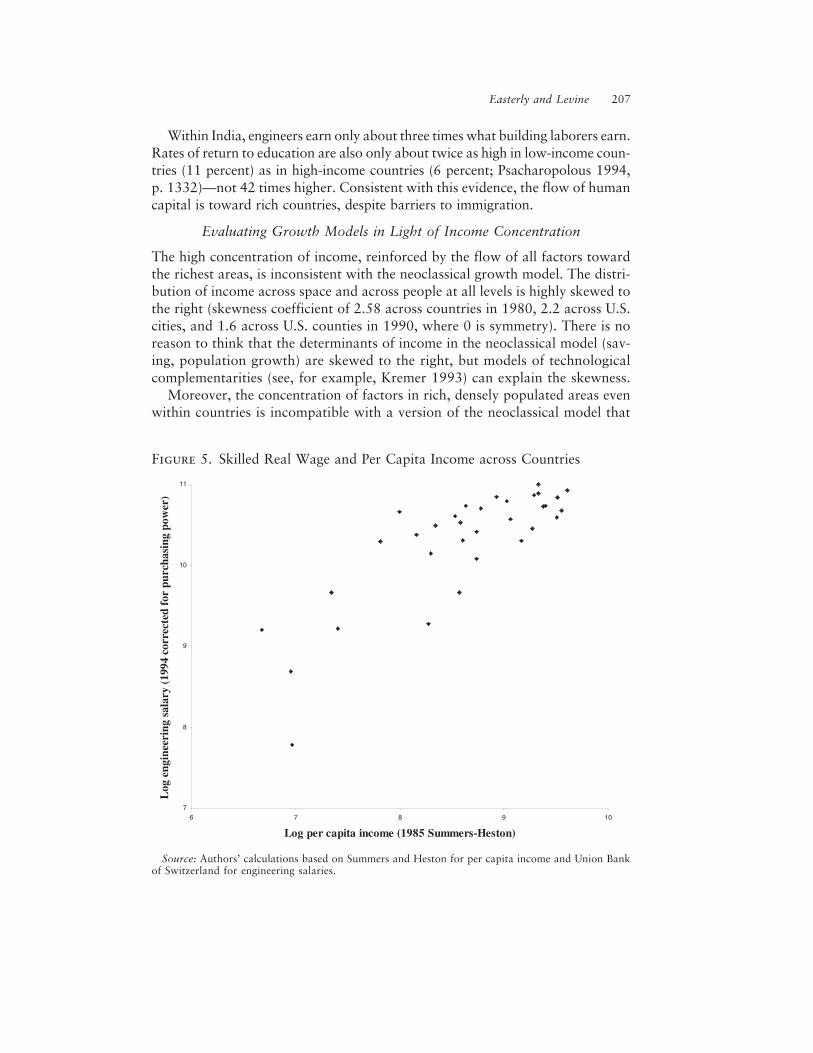
Easterly and Levine 207
Within India, engineers earn only about three times what building laborers earn.Rates of return to education are also only about twice as high in low-income coun-tries (11 percent) as in high-income countries (6 percent; Psacharopolous 1994,p. 1332)—not 42 times higher. Consistent with this evidence, the flow of humancapital is toward rich countries, despite barriers to immigration.
Evaluating Growth Models in Light of Income Concentration
The high concentration of income, reinforced by the flow of all factors towardthe richest areas, is inconsistent with the neoclassical growth model. The distri-bution of income across space and across people at all levels is highly skewed tothe right (skewness coefficient of 2.58 across countries in 1980, 2.2 across U.S.cities, and 1.6 across U.S. counties in 1990, where 0 is symmetry). There is noreason to think that the determinants of income in the neoclassical model (sav-ing, population growth) are skewed to the right, but models of technologicalcomplementarities (see, for example, Kremer 1993) can explain the skewness.
Moreover, the concentration of factors in rich, densely populated areas evenwithin countries is incompatible with a version of the neoclassical model that
7
8
9
10
11
6 7 8 9 10
Log per capita income (1985 Summers-Heston)
Log
eng
inee
ring
sal
ary
(199
4 co
rrec
ted
for
purc
hasi
ng p
ower
)
Figure 5. Skilled Real Wage and Per Capita Income across Countries
Source: Authors’ calculations based on Summers and Heston for per capita income and Union Bankof Switzerland for engineering salaries.

208 the world bank economic review, vol. 15, no. 2
includes land as a factor of production. With land in fixed supply, physical andhuman capital and labor should all flow to areas abundant in land (adjustingfor land quality) but scarce in other factors.
Furthermore, in the neoclassical model of Mankiw, Romer, and Weil (1992),physical and human capital should also flow from rich to poor areas, and unskilledlabor from poor to rich. But as this study shows, physical and human capital flowtoward rich areas, as does unskilled labor, though it is less mobile.
Stylized fact 4 is in harmony with Klenow and Rodriguez-Clare (1997b), whocomplain that the “neoclassical revival in growth economics” has “gone too far.”The neoclassical model does not explain why wealth and poverty are concen-trated in certain regions within countries or why there are such pronounced in-come differences between ethnic groups. Stylized fact 4 is consistent with pov-erty trap models (Azariadis and Drazen 1990, Becker, Murphy, and Tamura1990, Kremer 1993, Murphy, Shleifer, and Vishny 1989); with models of in-group ethnic and neighborhood externalities (Borjas 1992, 1995, 1999, Benabou1993, 1996), and with models of geographic externalities (Krugman 1991, 1995,1998, Fujita, Krugman, and Venables 1999).
Stylized fact 4 also seems to be more consistent with a productivity explana-tion of income differences than with a factor accumulation story. If a rich areais rich because technology (A) is more advanced, then all factors of productionwill tend to flow toward this rich area, reinforcing the concentration. Spilloversbetween agents also seem more natural with technological models of growth, astechnological knowledge is inherently more nonrival and nonexcludable thanfactor accumulation. Technological spillovers between agents will lead to en-dogenous matching of rich agents with each other, and those matches will rein-force the matching of poor people with other poor people (as in the O-ring storyof Kremer [1993] or the inequality model of Benabou [1996]). A better under-standing of economic geography and externalities would help shape more real-istic models of economic growth.
VI. Stylized Fact 5. Policy Matters
The empirical literature on national policies and economic growth is huge. Thereis considerable disagreement about which policies are most strongly linked witheconomic growth. Some analysts focus on openness to international trade (Frankeland Romer 1999), some on fiscal policy (Easterly and Rebelo 1993), some on fi-nancial development (Levine, Loayza, and Beck 2000), and some on macroeco-nomic policies (Fischer 1993). All these studies have at least one feature in com-mon: They all find that some indicator of national policy is strongly linked witheconomic growth, confirming the argument made by Levine and Renelt (1992).
Most empirical assessments of the growth-policy relationship are plagued bythree shortcomings. First, most do not confront endogeneity. Even when instru-mental variables are used, studies frequently assume that many of the regressorsare exogenous and focus only on the potential endogeneity of one variable of

Easterly and Levine 209
interest. This failure to fully confront causality may produce biased assessments.Second, traditional cross-country regressions may suffer from omitted variablebias. That is, cross-country growth regressions may omit an important country-specific effect and thereby produce biased coefficient estimates. Third, almostall cross-country regressions included lagged real per capita gdp as a regressor.Because the dependent variable is the growth rate of real per capita gdp, thisspecification may produce biased coefficient estimates.
This study uses recent econometric techniques to examine the links betweeneconomic growth and a range of national policies. These new techniques ame-liorate these potential biases so that more accurate inferences can be drawn aboutthe impact of national policies on economic growth. The goal is not to identifythe most important policies influencing growth; it is to compile key stylized factsassociated with long-run growth.
Use of the latest econometric techniques (see appendix) confirms earlier find-ings that national policies are strongly linked with economic growth. The re-gression results are consistent with policies having significant long-run effectson national growth rates or on steady-state levels of national output. The re-gression results also show that national policies are strongly linked with tfpgrowth (Beck, Levine, and Loayza 2000).
The relationship between the exogenous component of national policies andeconomic growth is assessed using a set of conditioning information and policyindicators suggested by theory and past empirical work. Specifically, the initiallevel of real income per capita is included to control for convergence. The stan-dard neoclassical growth model predicts convergence to the steady-state outputper person ratio (Barro and Sala-i-Martin 1995). The coefficient on initial incomedoes not necessarily capture only neoclassical transitional dynamics. In technol-ogy diffusion models, initial income may proxy for the initial gap in tfp betweeneconomies. In these models, therefore, catch-up can be in tfp as well as in tradi-tional factors of production. Average years of schooling was included as an indi-cator of the human capital stock in the economy. Its inclusion can help in control-ling for differences in steady-state levels of human capital (Barro and Sala-i-Martin1992). Also, schooling may directly influence economic growth (Lucas 1988).
Five policy indicators were used. The inflation rate and the ratio of governmentexpenditures to gdp were included as indicators of macroeconomic stability (East-erly and Rebelo 1993, Fischer 1993). Exports plus imports as a share of gdp andthe black market exchange rate premium were included to capture degree of open-ness (Frankel and Romer 1999). Financial intermediary credit to the private sec-tor as a share of gdp was included as a measure of financial intermediary develop-ment (Levine, Loayza, and Beck 2000). There is no attempt to suggest that theseare the most important policy indicators. They are used only to assess whethereconomic growth is strongly linked with these national policy indicators aftercontrolling for endogeneity and other biases in existing empirical work.
As in much of the cross-country literature, the regression results show evi-dence of conditional convergence (table 7). Specifically, contingent of the level

210 the world bank economic review, vol. 15, no. 2
of human capital, poorer countries tend to grow faster than richer countries aseach country converges toward its steady-state. This finding is consistent with amajor implication of the textbook neoclassical growth model. The regression alsoshows that greater human capital—as measured by average years of schoolingof the working age population—is associated with faster economic growth.Moreover, since the gmm panel estimator controls for endogeneity, this findingsuggests that the exogenous component of schooling exerts a positive impact oneconomic growth. These results are consistent with models that focus on factoraccumulation or on tfp growth.
The results are consistent with—but not proof of—long-run growth effectsof national policies, which is consistent with an endogenous productivity growthmodel. In contrast, models that feature only transitional factor accumulationdynamics usually predict weaker policy effects on growth than endogenous pro-ductivity growth models. Furthermore, complementary work in Beck, Levine,and Loayza (2000) suggests a powerful connection between national policies andtfp growth. The exogenous components of international openness—as measured
Table 7. Economic Growth and National Policies
Variable Result
Constant 0.082 (0.875)Initial income per capitaa –0.496 (0.001)Average years of schoolingb 0.950 (0.001)Openness to tradea 1.311 (0.001) Inflationb 0.181 (0.475)Government sizea –1.445 (0.001) Black market premiumb –1.192 (0.001)Private credita 1.443 (0.001)Sargan testc (p-value) 0.506Serial correlation testd (p-value) 0.803
Note: Numbers in parentheses are p-values. The dependentvariable is real per capita gdp growth.
aIncluded as log(variable).bIncluded as log(1 + variable).cThe null hypothesis is that the instruments used are not cor-
related with the residuals.dThe null hypothesis is that the errors in the first-difference
regression exhibit no second-order serial correlation.Source: Authors’s calculations based on analyses in Beck, Levine,
and Loayza (2000).

Easterly and Levine 211
by the ratio of trade to gdp and by black market exchange rate premia—aresignificantly correlated with economic growth.
Macroeconomic policy is also important. Large government tends to hurteconomic growth, although inflation does not enter significantly. A higher blackmarket exchange rate premium exerts a negative impact on growth. More inter-national trade tends to boost economic growth. While considerable researchsuggests a negative link between inflation and economic performance (Bruno andEasterly 1998), recent research suggests that inflation is strongly linked with fi-nancial development (Boyd, Levine, and Smith 2001). Thus, it may not enjoy anindependent link with growth when financial development is controlled for. Fi-nally, a higher level of financial development boosts economic growth. In sum,national policies are strongly linked with economic growth.
VII. Conclusion
The major empirical regularities of economic growth emphasize the role of some-thing else besides factor accumulation. The tfp residual accounts for most of thecross-country and cross-time variation in growth. Income across countries divergesover the long run, while the growth rates of the rich are not slowing and returns tocapital are not falling. This observation is less consistent with simple models thatfeature diminishing returns, factor accumulation, some fixed factor of production,and constant returns to scale and more consistent with the observation that some-thing else is important for explaining long-run economic success. Growth is highlyunstable over time, whereas factor accumulation is more stable, which certainlyemphasizes the role of something else in explaining variations in economic growth.All factors of production flow to the richest areas, suggesting that they are richbecause of high A rather than high K. Divergence of per capita incomes and theconcentration of economic activity suggest that technology has increasing returns.Finally, national policies are strongly linked with long-run economic growth rates.
Nothing in this study argues that factor accumulation is unimportant in gen-eral or denies that it is critically important for some countries at specific junc-tures. tfp does not explain everything, everywhere, always. Rather, the studyshows that something else—besides factor accumulation—plays a prominent rolein explaining differences in economic performance across countries.
More research is needed on the “residual” determinants of growth and in-come, such as technology and externalities. There is little doubt that technologyis a formidable force. Nordhaus (1994) estimates that 1 Btu of fuel consump-tion today buys 900 times more lighting (measured in lumen hours) than it didin 1800. Over the past two decades, computing power per dollar invested hasrisen by a factor of 10,000, and the cost of sending information over optical fiberhas fallen by a factor of 1,000 (World Bank 1999, pp. 5 and 57). Just from 1991to 1998, the price of a megabyte of hard disk storage fell from $5 to $0.03.28
28. www.duke.edu/~mccann/q-tech.htm#Death of Distance.

212 the world bank economic review, vol. 15, no. 2
Not every technology has improved at this speed of course. But Mokyr (1992)was right to call technology “the lever of riches.”
Appendix: Econometric Methodology
A generalized method of moments (gmm) dynamic panel estimator was usedto assess the relationship between policy and economic growth. Panel data for73 countries over the period 1960–95 were averaged over seven nonoverlappingfive-year periods.
Consider the following equation:
(13) yi,t – yi,t–1 = (a – 1)yi,t–1 + b'Xi,t + hi +ei,t
where y is the logarithm of real per capita gdp, X is the set of explanatory vari-ables (other than lagged per capita gdp), h is an unobserved country-specific effect,e is the error term, and the subscripts i and t represent country and time period.Time dummy variables were also included to account for time-specific effects.
Equation 13 can be rewritten as:
(14) yi,t = ayi,t–1 + b'Xi,t + hi +ei,t.
First differences of equation 14 are taken to eliminate the country-specific effect:
(15) yi,t – yi,t–1 = a(yi,t–1 – yi,t–2) + b'(Xi,t + Xi,t–1) + (ei,t – ei,t–1).
The use of instruments is required to deal with the correlation, by construction,of the new error term ei,t – ei,t–1 with the lagged dependent variable yi,t–1 – yi,t–2
and with the likely endogeneity of the explanatory variables. Under the tested as-sumptions that the error term (e) is not serially correlated and the explanatoryvariables (X) are weakly exogenous (the explanatory variables are assumed to beuncorrelated with future realizations of the error term), appropriately lagged val-ues of the regressors can be used as instruments, as specified in the followingmoment conditions:
(16) E[yi,t–s · (ei,t – ei,t–1)] = 0 for s ≥ 2; t = 3, . . . , T
(17) E[Xi,t–s · (ei,t – ei,t–1)] = 0 for s ≥ 2; t = 3, . . . , T.
The gmm estimator based on these conditions is referred to as the differenceestimator.
There are, however, conceptual and statistical shortcomings with this differ-ence estimator. It eliminates the cross-country relationship between national poli-cies and per capita gdp growth, which is of conceptual interest. Statistically, whenthe regressors in equation 15 are persistent, lagged levels of X and y are weak in-struments. Instrument weakness influences the asymptotic and small-sample per-formance of the difference estimator. Asymptotically, the variance of the coefficientsrises. In small samples, weak instruments can produce biased coefficients.
To reduce the potential biases and imprecision associated with the usual dif-ference estimator, Arellano and Bover (1995) and Blundell and Bond (1997)

Easterly and Levine 213
develop a system of regressions in differences and levels. The instruments forthe regression in differences are the same as those above. The instruments forthe regression in levels are the lagged differences of the corresponding variables.These are appropriate instruments under the following additional assumption:although there may be correlation between the levels of the right-hand-side vari-ables and the country-specific effect in equation 14, there is no correlation be-tween the differences of these variables and the country-specific effect. This as-sumption results from the following stationarity property:
(18) E[yi,t+p · hi] = E[yi,t+q · hi]and E[Xi,t+p · hi] = E[Xi,t+q · hi] for all p and q.
The additional moment conditions are.
(19) E[(yi,t–s – yi,t–s–1)·(hi + ei,t)] = 0 for s = 1
(20) E[(Xi,t–s – Xi,t–s–1)·(hi + ei,t)] = 0 for s = 1.
Thus the moment conditions presented in equations 16, 17, 19, and 20 are usedwith a gmm estimator to generate consistent and efficient parameter estimates.
Consistency of the gmm estimator depends on the validity of the instruments.To address this issue two specification tests were considered, as suggested byArellano and Bond (1991), Arellano and Bover (1995), and Blundell and Bond(1997). The first is a Sargan test of overidentifying restrictions to test the overallvalidity of the instruments by analyzing the sample analog of the moment con-ditions used in the estimation. The second test examines the hypothesis thatthe error term ei,t is not serially correlated. In both the difference regressionand the system regression the differenced error term is tested for second-orderserial correlation (by construction, the differenced error term is probably first-order serially correlated even if the original error term is not). This system es-timator is used to assess the impact of policies on economic growth. In addi-tion to the system estimator, the analyses use purely cross-section, ordinaryleast squares regressions with one observation per country, the pure differentestimator described above, and the panel estimator with only the level compo-nent of the system estimator. All yield similar results and parameter values(Levine, Loayza, and Beck 2000).
References
Ades, Alberto, and Edward Glaeser. 1999. “Evidence on Growth, Increasing Returns,and the Extent of the Market.” Quarterly Journal of Economics 114(3):1025–46.
Aghion, P., and P. Howitt. 1998. Endogenous Growth Theory. Cambridge, Mass.: mitPress.
Alesina, Alberto, Reza Baqir, and William Easterly. 1999. “Public Goods and EthnicDivisions.” Quarterly Journal of Economics 114(4):1243–84.

214 the world bank economic review, vol. 15, no. 2
Arellano, Manuel, and Bond, Stephen. “Some Tests of Specification for Panel Data. MonteCarlo Evidence and an Application to Employment Equations.” Review of EconomicStudies 58(2):277–97.
Arellano, Manuel, and Bover, Olympia. 1995. “Another Look at the Instrumental-Vari-able Estimation of Error-Components Models.” Journal of Econometrics 68(1):29–52.
Azariadis, Costas, and Allan Drazen. 1990. “Threshold Externalities in Economic De-velopment,” Quarterly Journal of Economics 105:501–26.
Bairoch,Paul. 1993. Economics and World History: Myths and Paradoxes. Chicago:University of Chicago Press.
Baldwin, Richard E. 1998. “Global Income Divergence, Trade and Industrialization. TheGeography of Growth Take-offs.” nber Working Paper Series No. 6458.1. nber, Wash-ington, D.C.
Bank for International Settlements. 1996. 66th Annual Report. bis, Basel.Barro, Robert, and Xavier Sala-i-Martin. 1992. “Convergence.” Journal of Political
Economy 100(2):223–51.———. 1995. Economic Growth. New York: McGraw-Hill.Barro, Robert, J. Mankiw, N. Gregory, and X. Sala-i-Martin. 1995. “Capital Mobility
in Neoclassical Models of Growth.” American Economic Review 85:103–15.Baumol, William J. 1986. “Productivity Growth, Convergence, and Welfare. What the
Long Run Data Show.” American Economic Review 76(5):1072–85.Beck, Thorsten. Ross Levine, and Norman Loayza. 2000. “Finance and the Sources of
Growth.” Journal of Financial Economics 58(1–2):261–300.Becker, Gary S., Kevin M. Murphy, and Robert Tamura. 1990. “Human Capital, Fertil-
ity, and Economic Growth.” Journal of Political Economy 98(5):S12–S37.Benabou, Roland. 1993. “Workings of a City. Location, Education, and Production.”
Quarterly Journal of Economics 108:619–52.———. 1996. “Heterogeneity, Stratification, and Growth. Macroeconomic Implications
of Community Structure and School Finance.” American Economic Review 86(3):584–609.
Benhabib. J., and M. Spiegel. 1994. “Role of Human Capital in Economic Development.Evidence from Aggregate Cross-Country Data.” Journal of Monetary Economics34:143–73.
Bils, Mark, and P. Klenow. 1996. “Does Schooling Cause Growth?” American EconomicReview 90(5.):1160–83.
Blomstrom, Magnus, R. Lipsey, and M. Zejan. 1996. “Is Fixed Investment the Key toEconomic Growth?” Quarterly Journal of Economics 111(1):269–76.
Blundell, Richard, and Bond, Stephen. 1997. “Initial Conditions and Moment Restrictionsin Dynamic Panel Data Models.” University College London Discussion Paper 97-07.
Borjas, George J. 1992. “Ethnic Capital and Intergenerational Mobility.” QuarterlyJournal of Economics 107:123–50.
———. 1995. “Ethnicity, Neighborhoods, and Human Capital Externalities.” Ameri-can Economic Review 85(3):365–90.
———. 1999. Heaven’s Door. Immigration Policy and the American Economy. Princeton,N.J.: Princeton University Press.
Borjas, George J., Stephen G. Bronars, and Stephen J. Trejo. 1992. “Self Selection andInternal Migration in the United States.” Journal of Urban Economics 32:159–85.
Easterly and Levine 215
Bouillon, César, Arianna Legovini, and Nora Lustig. 1999. “Rising Inequality in Mexico,Returns to Household Characteristics and the ‘Chiappas’ Effect.” Inter-AmericanDevelopment Bank, mimeo.
Boyd, John H., Ross Levine, Bruce D. Smith. 2001. “The Impact of Inflation on Finan-cial Sector Performance.” Journal of Monetary Economics. Forthcoming.
Brookings Institution Center on Urban and Metropolitan Policy. 1999. A Region Di-vided. The State of Growth in Greater Washington. Washington, D.C.: BrookingsInstitution.
Bruno, Michael, and Easterly, William. 1998. “Inflation Crises and Long-run Growth.”Journal of Monetary Economics 41:3–26.
Burnside, Craig. 1996. “Production Function Regressions, Returns to Scale and Exter-nalities.” Journal of Monetary Economics 37:177–200.
Carrington, William J., and Enrica Detragiache. 1998. “How Big Is the Brain Drain?”International Monetary Fund Working Paper 98/102.
Carroll, C. D., and D. N. Weil. 1993. “Saving and Growth. A Reinterpretation.” Carnegie-Rochester Series on Public Policy.
Ciccone, Antonio, and Robert E. Hall. 1996. “Productivity and the Density of EconomicActivity.” American Economic Review 86(1):54–70.
Collier, Paul, David Dollar, and Nicholas Stern. 2000. “Fifty Years of Development.”World Bank, mimeo.
Costello, Donna M. 1993. “Cross-Country, Cross-Industry Comparison of ProductivityGrowth.” Journal of Political Economy 101:207–22.
Christiansen, L. R. D. Cummings, and D. Jorgenson. 1980. “Economic Growth, 1947—1973: An International Comparison.” In J. W. Kendrick and B. Vaccara (eds.), NewDevelopments in Productivity Measurement and Analysis. Studies in Income andWealth, Vol. 41, Chicago: University of Chicago Press.
De Long, J. Bradford. 1988. “Productivity Growth, Convergence, and Welfare. Com-ment.” American Economic Review 78(5):1138–54.
Denison, Edward F. 1962. Sources of Economic Growth in the United States and theAlternatives Before Us. New York. Committee for Economic Development.
———. 1967. Why Growth Rates Differ. Washington, D.C. Brookings Institution.Dougherty, Christopher. 1991. A Comparison of Productivity and Economic Growth
in the G-7 Countries. Ph.D. dissertation, Harvard University.Easterly, William. 1999a. “The Ghost of Financing Gap. Evaluating the Growth Model
of the International Financial Institutions.” Journal of Development Economics,December.
———. 1999b. “Life During Growth.” Journal of Economic Growth 4(3):239–76.———. 2001. “The Lost Decades. Developing Countries’ Stagnation in Spite of Policy
Reform 1980–98.” Journal of Economic Growth 6(2):135–57.Easterly, William, and Sergio Rebelo. 1993. “Fiscal Policy and Economic Growth. An
Empirical Investigation.” Journal of Monetary Economics 32:417–58.Easterly, William, Michael Kremer, Lant Pritchett, and Lawrence Summers. 1993. “Good
Policy or Good Luck? Country Growth Performance and Temporary Shocks.” Jour-nal of Monetary Economics 32:459–83.
Elias, Victor J. 1990. Sources of Growth. A Study of Seven Latin American Economies.International Center for Economic Growth.

216 the world bank economic review, vol. 15, no. 2
Fischer, Stanley. 1993. “The Role of Macroeconomic Factors in Growth.” Journal ofMonetary Economics 32:485–512.
Frarikel, J. A., and David Romer. 1999. “Does Trade Cause Growth?” American Eco-nomic Review 89:379–99.
Fujita, Masahisa, Paul Krugman, and Anthony Venables. 1999. The Spatial Economy:Cities, Regions, and International Trade. Cambridge, Mass.: MIT Press.
Grossman, G., and E. Helpman. 1991. “Quality Ladders in the Theory of EconomicGrowth.” Review of Economic Studies 58:43–61.
Grubel, Herbert G., and Anthony Scott. 1977. The Brain Drain. Determinants, Mea-surement and Welfare Effects. Waterloo, Ontario: Wilfrid Laurier University Press.
Hadjmichael, Michael T., Michael Nowak, Robert Sharer, and Amor Tahari. 1996.Adjustment for Growth. The African Experience. Washington, D.C.: imf.
Hall, Robert E., and Charles Jones. 1999. “Why Do Some Countries Produce So MuchMore Output per Worker than Others?” Quarterly Journal of Economics 114(1):83–116.
Hansen, Gary D., and Edward Prescott. 1998. “Malthus to Solow.” nber WorkingPaper Series No. 6858.1–24.
Hanushek, Eric A., and Dennis D. Kimko. 2000. “Schooling, Labor-Force Quality, andthe Growth of Nations.” American Economic Review 90(5):1184–1208.
Harberger, Arnold C. 1998. “A Vision of the Growth Process.” American EconomicReview 88(1):1–32.
Holmes, T., and J. A. Schmitz Jr. 1995. “Resistance to New Technologies and Tradebetween Areas.” Federal Reserve Bank of Minneapolis Quarterly Review 19:2–18.
International Labor Organization. 1995. World Employment. Geneva.Jalan, Jyotsna, and Martin Ravallion. 1997. “Spatial Poverty Traps?” World Bank Policy
Research Working Paper No. 1862.Jones, Charles. 1995a. “R&D-Based Models of Economic Growth.” Journal of Political
Economy 103:759–84.———. 1995b. “Time Series Tests of Endogenous Growth Models.” Quarterly Journal
of Economics 105(2):495–526.———. 1997. “Comment on Peter Kienow and Andres Rodriguez-Clare, ‘The Neoclas-
sical Revival in Growth Economics. Has It Gone Too Far?’” NBER MacroeconomicsAnnual 12:73–103.
———. 1999. “Was an Industrial Revolution Inevitable? Economic Growth Over theVery Long Run.” Stanford University, mimeo.
Jorgenson, Dale W. 1995. Productivity. Cambridge, Mass.: mit Press.Kendrick, John W., and Elliot S. Grossman. 1980. Productivity in the United States:
Trends and Cycles. Baltimore, Md.: Johns Hopkins University Press.King, Robert G., and Ross Levine. 1994. “Capital Fundamentalism, Economic Develop-
ment and Economic Growth.” Carnegie-Rochester Conference Series on Public Policy40:259–92.
King, Robert G., and Sergio Rebelo. 1993. “Transitional Dynamics and Economic Growthin the Neoclassical Model.” American Economic Review 83:908–31.
Klenow, Peter. 1998. “Ideas versus Rival Human Capital. Industry Evidence on GrowthModels.” Journal of Monetary Economics 42:2–23.

Easterly and Levine 217
Klenow. Peter, and Andres Rodriguez-Clare. 1997a. “Economic Growth. A Review Es-say.” Journal of Monetary Economics 40:597–617.
———. 1997b. “The Neoclassical Revival in Growth Economics. Has It Gone Too Far?”nber Macroeconomics Annual 12:73–103.
Klitgaard, Robert, and Amand Fitschen. 1997. “Exploring Income Variations acrossTraditional Authorities in KwaZulu-Natal, South Africa.” Development SouthernAfrica 14(3).
Kongsamut, Piyabha, Sergio Rebelo, and Danyang Xie. 1997. “Beyond Balanced Growth.”University of Rochester Working Paper.
Kosmin, Barry A., and Seymour P. Lachman. 1993. One Nation under God. Religion inContemporary American Society. New York: Harmony Books.
Kremer, Michael. 1993. “O-ring Theory of Economic Development.” Quarterly Jour-nal of Economics 108:551–75.
Krueger, Alan B., and Mikael Lindahl. 1999. “Education for Growth in Sweden and theWorld.” nber Working Paper Series No. 7190.1–54.
Krugman, Paul R. 1991. Geography and Trade. Cambridge, Mass.: mit Press.———. 1995. Development, Geography, and Economic Theory. Cambridge, Mass.: mit
Press.———. 1998. “Space. The Final Frontier.” Journal of Economic Perspectives 12:161–74.Krugman, Paul R., and Anthony J. Venables. 1995. “Globalization and the Inequality
of Nations.” Quarterly Journal of Economics 110(4):857–80.Lipset, Seymour Martin. 1997. American Exceptionalism. A Double Edged Sword. New
York: Norton.Levine, Ross, and David Renelt. 1992. “A Sensitivity Analysis of Cross-Country Growth
Regressions.” American Economic Review 82(4):942–63.Levine, Ross, Norman Loayza, and Thorsten Beck. 2000. “Financial Intermediation and
Growth. Causality and Causes.” Journal of Monetary Economics 46:31–77.Lewis, W. A. 1954. “Economic Development with Unlimited Supplies of Labor.”
Manchester School of Economic and Social Studies 22(2):139–91.Lucas, Robert E., Jr. 1988. “On the Mechanics of Economic Development.” Journal of
Monetary Economics 22:3–42.———. 1990. “Why Doesn’t Capital Flow from Rich to Poor Countries?” American
Economic Review, Papers and Proceedings 80:92–96.———. 1998. “The Industrial Revolution. Past and Future.” Mimeo, University of Chicago.Maddison. Angus. 1995. Monitoring the World Economy, 1820–1992. Paris: Develop-
ment Centre of the Organisation for Economic Co-operation and Development.Mankiw, N. Gregory. 1995. “The Growth of Nations.” Brookings Papers on Economic
Activity 1:275–326.Mankiw, N. Gregory, David Romer, and David N. Weil. 1992. “Contribution to the
Empirics of Economic Growth.” Quarterly Journal of Economics 107:407–37.McGrattan, Ellen R. 1998. “A Defense of ak Growth Models.” Quarterly Review, Fed-
eral Reserve Bank of Minneapolis 22:13–27.Mellinger, Andrew D., Jeffrey D. Sachs, and John L. Gallup. 1999. “Climate, Water
Navigability, and Economic Development.” Harvard Center for International Devel-opment Working Paper No. 24.

218 the world bank economic review, vol. 15, no. 2
Mokyr, Joel. 1992. The Lever of Riches. Technological Creativity and Economic Progress.New York: Oxford University Press.
Murphy, Kevin M., Andrei Shleifer, and Robert Vishny. 1989. “Industrialization andthe Big Push.” Journal of Political Economy 97:1003–26.
Nehru, Vikram, and A. Dhareshwar. 1993. “A New Database on Physical Capital Stocks.Sources, Methodology, and Results.” Revista de Análisis Económico 8(1):37–60.
Nordhaus, William. 1994. “Do Real Output and Real Wage Measures Capture Reality?The History of Lighting Suggests Not.” Yale Cowles Foundation Discussion Paper 1078.
Parente, Stephen. 1994. “Technology Adoption, Learning-by-Doing, and EconomicGrowth.” Journal of Economic Theory 63:346–69.
Parente, S. L., and E. C. Prescott. 1996. “Barriers to Technology Adoption and Devel-opment.” Journal of Political Economy l02(2):298–321.
Patrinos, Harry Anthony. 1997. “Differences in Education and Earnings across EthnicGroups in Guatemala.” Quarterly Review of Economics and Finance 37(4):807–21.
Prescott, Edward. 1998. “Needed. A Theory of Total Factor Productivity.” InternationalEconomic Review 39(3):525–32.
Pritchett, Lant. 1997. “Divergence, Big Time.” Journal of Economic Perspectives 11(3):3–17.
———. 1999. “The Tyranny of Concepts. CUDIE (Cumulated, Depreciated, InvestmentEffort) Is Not Capital.” World Bank, mimeo.
———. 2000. “Patterns of Economic Growth. Hills, Plateaus, and Mountains.” WorldBank Economic Review 14(2):221–49.
———. 2001. “Where Has All the Education Gone?” World Bank Economic Review.Forthcoming.
Psacharopoulos, George. 1994. “Returns to Investment in Education. A Global Update.”World Development 22:1325–1343.
Quah, Danny. 1993. “Galton’s Fallacy and Tests of the Convergence Hypothesis.” Scan-dinavian Journal of Economics 95(4):427–43.
Rappaport, Jordan, and Jeffrey Sachs. 1999. “The United States as a Coastal Nation.”Harvard Center for International Development, mimeo.
Rauch, James E. 1993. “Productivity Gains from Geographic Concentration of HumanCapital. Evidence from the Cities.” Journal of Urban Economics 34:380–400.
Ravallion, Martin, and Jyotsna Jalan. 1996. “Growth Divergence Due to Spatial Exter-nalities.” Economics Letters 53:227–32.
Ravallion, Martin, and Quentin Wodon. 1998. “Poor Areas or Only Poor People?” WorldBank, mimeo.
Ray, Debraj. 1998. Development Economics. Princeton, N.J.: Princeton University Press.Rebelo, Sergio, and Nancy L. Stokey. 1995. “Growth Effects of Flat-Rate Taxes.” Jour-
nal of Political Economy 103:519–50.Rodrik, Dani. 1998. “Where Did all the Growth Go? External Shocks, Social Conflict
and Growth Collapses.” nber Working Paper Series No. 6350.Romer, Paul. 1986. “Increasing Returns and Long-Run Growth.” Journal of Political
Economy 94:1002–37.———. 1990. “Endogenous Technological Change.” Journal of Political Economy
98:S71–S102.

Easterly and Levine 219
———. 1995. “Comment on N. Gregory Mankiw, ‘The Growth of Nations’” BrookingsPapers on Economic Activity 1:313–20.
Rostow, W. W. 1960. The Stages of Economic Growth. A Non-Communist Manifesto.Cambridge: Cambridge University Press.
Shleifer, Andrei, and Robert Vishny. 1993. “Corruption.” Quarterly Journal of Econom-ics 108(3):599–667.
Solow, R. 1956. “A Contribution to the Theory of Economic Growth.” Quarterly Jour-nal of Economics 70:65–94.
———. 1957. “Technical Change and the Aggregate Production Function.” Review ofEconomics and Statistics 39:312–20.
Todaro, Michael P. 2000. Economic Development, 7th ed. Reading, Mass.: Addison-Wesley.
Union Bank of Switzerland. 1994. Prices and Earnings around the Globe. Zurich: UnitedBank of Switzerland.
United Nations. 1996. World Economic and Social Survey.United States Government. 1996. 1995 Statistical Abstract of US. Washington, D.C.World Bank. 1993. The East Asian Miracle. Washington, D.C.: World Bank.———. 1995. Latin America after Mexico. Quickening the Pace. Washington, D.C.:
World Bank.———. 1999. World Development Report. Oxford: Oxford University Press.———. 2000a. Can Africa Claim the 21st Century? Washington, D.C.: World Bank.———. 2000b. East Asia. Recovery and Beyond. Washington, D.C.: World Bank.———. 2000c. The Road to Stability and Prosperity in South Eastern Europe. Europe
and Central Asia Region, Washington, D.C.: World Bank.———. 2000/2001. World Development Report. Attacking Poverty. Washington, D.C.:
World Bank.Young, Alwyn. 1995. “The Tyranny of Numbers: Confronting the Statistical Realities
of the East Asian Growth Experience.” Quarterly Journal of Economics 110:641–80.