isotopic signatures of production and uptake of h2 by soil

Atmos. Chem. Phys., 15, 13003–13021, 2015

www.atmos-chem-phys.net/15/13003/2015/

doi:10.5194/acp-15-13003-2015

© Author(s) 2015. CC Attribution 3.0 License.

Isotopic signatures of production and uptake of H2 by soil

Q. Chen1,2, M. E. Popa1, A. M. Batenburg1,3, and T. Röckmann1

1Institute for Marine and Atmospheric research Utrecht, Utrecht University, Utrecht, the Netherlands2Department of Atmospheric Sciences, University of Washington, Seattle, Washington, USA3Department of Applied Physics, University of Eastern Finland, Kuopio, Finland

Correspondence to: Q. Chen ([email protected])

Received: 17 April 2015 – Published in Atmos. Chem. Phys. Discuss.: 1 September 2015

Revised: 11 November 2015 – Accepted: 12 November 2015 – Published: 24 November 2015

Abstract. Molecular hydrogen (H2) is the second most abun-

dant reduced trace gas (after methane) in the atmosphere, but

its biogeochemical cycle is not well understood. Our study

focuses on the soil production and uptake of H2 and the

associated isotope effects. Air samples from a grass field

and a forest site in the Netherlands were collected using

soil chambers. The results show that uptake and emission

of H2 occurred simultaneously at all sampling sites, with

strongest emission at the grassland sites where clover (N2

fixing legume) was present. The H2 mole fraction and deu-

terium content were measured in the laboratory to deter-

mine the isotopic fractionation factor during H2 soil uptake

(αsoil) and the isotopic signature of H2 that is simultane-

ously emitted from the soil (δDsoil). By considering all net-

uptake experiments, an overall fractionation factor for de-

position of αsoil = kHD / kHH = 0.945± 0.004 (95 % CI) was

obtained. The difference in mean αsoil between the forest soil

0.937± 0.008 and the grassland 0.951± 0.026 is not statis-

tically significant. For two experiments, the removal of soil

cover increased the deposition velocity (vd) and αsoil simul-

taneously, but a general positive correlation between vd and

αsoil was not found in this study. When the data are evaluated

with a model of simultaneous production and uptake, the iso-

topic composition of H2 that is emitted at the grassland site is

calculated as δDsoil = (−530± 40) ‰. This is less deuterium

depleted than what is expected from isotope equilibrium be-

tween H2O and H2.

1 Introduction

H2 is considered an alternative energy carrier to replace fos-

sil fuels in the future. However, the environmental and cli-

mate impact of a potential widespread use of H2 is still under

assessment. Several studies suggested that the atmospheric

H2 mole fraction might increase substantially in the future

due to the leakage during production, storage, transportation

and use of H2, which could significantly affect atmospheric

chemistry (Schultz et al., 2003; Tromp et al., 2003; Van Rui-

jven et al., 2011; Warwick et al., 2004).

In the troposphere, H2 has a mole fraction of about

550 parts per billion (ppb= nmol mol−1) and a lifetime of

around 2 years (Novelli et al., 1999; Price et al., 2007; Xiao

et al., 2007; Pieterse et al., 2011; 2013). H2 can affect atmo-

spheric chemistry and composition in several ways. Firstly, it

increases the lifetime of the greenhouse gas methane (CH4)

via its competing reaction with the hydroxyl radical (OH)

(Schultz et al., 2003; Warwick et al., 2004). Additionally, H2

affects air quality because it is an ozone (O3) precursor and

indirectly increases the lifetime of the air pollutant carbon

monoxide (CO) through competition for OH. In the strato-

sphere, H2O that is produced through the oxidation of H2

increases humidity, which can result in increased formation

of polar stratospheric clouds and O3 depletion (Tromp et al.,

2003), but this effect may be weaker than estimated initially

(Warwick et al., 2004; Vogel et al., 2012).

The main sources of tropospheric H2 are the oxidation

of CH4 and non-methane hydrocarbons (NMHC) (48 %),

biomass burning (19 %), fossil fuel combustion (22 %) and

biogenic N2 fixation in the ocean (6 %) and on land (4 %),

while the main sinks are soil uptake (70 %) and oxidation by

OH (30 %) (Pieterse et al., 2013).

Published by Copernicus Publications on behalf of the European Geosciences Union.

13004 Q. Chen et al.: Isotopic signatures of production and uptake of H2 by soil

The biogenic soil sink of H2 is the largest and most uncer-

tain term in the global atmospheric H2 budget. Conrad and

Seiler (1981) assumed that the soil uptake of atmospheric

H2 is most likely due to consumption by abiotic enzymes,

since there were no soil microorganisms known to be able

to fix H2 at the low atmospheric mole fraction at that time.

This remained the basic hypothesis of many further soil up-

take studies (Conrad et al., 1983; Conrad and Seiler, 1985;

Ehhalt and Rohrer, 2011; Guo and Conrad, 2008; Häring et

al., 1994; Smith-Downey et al., 2006). However, Constant

et al. (2008a) were first to identify an aerobic microorgan-

ism (Streptomyces sp. PCB7) that can consume H2 at tro-

pospheric ambient mole fractions and suggested that active

metabolic cells could be responsible for the soil uptake of

H2 rather than extracellular enzymes. Further studies showed

that uptake activity at ambient H2 level is widespread among

the streptomycetes (Constant et al., 2010) and it was postu-

lated that high-affinity H2-oxidizing bacteria are the main bi-

ological agent responsible for the soil uptake of atmospheric

H2 (Constant et al., 2011). Khdhiri et al. (2015) suggested

that the relative abundance of high-affinity H2-oxidation bac-

teria and soil carbon content could be used as predictive pa-

rameters for the H2-oxidation rate. Determining the domi-

nant mechanism of the H2 soil uptake activity is still an active

area of research.

It has been shown that soil uptake of H2 can coexist with

soil production (Conrad, 1994). H2 is produced in the soil

during N2 fixation (e.g., by bacteria living symbiotically in

the roots of legumes such as clover or beans) and dark fer-

mentation. Although the H2 produced in the soil by, e.g., N2

fixation can be largely consumed within the soil, a significant

amount of H2 escapes to the atmosphere (Conrad and Seiler,

1979, 1980). Conrad and Seiler (1980) estimated that 2.4 to

4.9 Tg a−1 of H2 is emitted into the atmosphere through N2

fixation on land.

One approach to better understand the sources and sinks

of H2 is to investigate the isotopic fractionation processes

involved, which act as a fingerprint for H2 emitted from dif-

ferent sources or destroyed by different sinks. The isotopic

composition of H2 is expressed as

δ(D,H2)=Rsa

RVSMOW

− 1,

where Rsa is the D /H ratio of the sample H2

and RVSMOW = (155.76± 0.8) parts per million

(ppm=mmol mol−1) is the same ratio of the standard

material, Vienna Standard Mean Ocean Water (VSMOW)

(De Wit et al., 1980; Gonfiantini et al., 1993). For brevity,

we will use the notation δD (= δD(D, H2)) throughout the

rest of this paper. The δD values are usually given in per mill

(‰). Recent studies showed that the global mean δD value

of atmospheric H2 is about+130 ‰ (Batenburg et al., 2011;

Gerst and Quay, 2000, 2001; Rice et al., 2010).

The HH molecule is consumed preferentially over HD dur-

ing both OH oxidation and soil uptake, with OH oxidation

causing a much stronger isotope fractionation effect. Only

a few studies have investigated the soil uptake of H2 with

isotope techniques. Gerst and Quay (2001) carried out field

experiments in Seattle, USA, and found αsoil (= kHD / kHH)

to be 0.943± 0.024 (1σ ). Note that kHD and kHH are re-

moval rate constants for HD and HH, respectively. Rahn et

al. (2002a) collected air samples from four forest sites in

ecosystems of different ages in Alaska, USA, in July 2001

and obtained a similar average value (0.94± 0.01). They sug-

gested that αsoil depends on the forest maturity, with smaller

fractionation for more mature forests. Since the more ma-

ture forests showed larger deposition velocity (vd) of H2,

they further suggested that lower uptake rates involve greater

isotopic fractionation (αsoil further from 1) than fast uptake

rates. Rice et al. (2011) performed deposition experiments in

Seattle and found αsoil varying from 0.891 to 0.976, with a

mean of 0.934. They found αsoil to be correlated with vd, with

smaller isotope effects (αsoil closer to 1) occurring at higher

vd, which agreed with the suggestion by Rahn et al. (2002a).

In addition, unpublished experiments from Rahn et al. (2005)

yielded αsoil = 0.89± 0.03 in three upland ecosystems that

were part of an Alaskan fire chronosequence. The data sug-

gest that variability in the soil/ecosystem affects αsoil but no

significant variability of αsoil with season was detected. Hith-

erto, only αsoil values from studies in Seattle and Alaska are

available, and values from other locations and ecosystems are

needed to learn more about the factors influencing αsoil.

The δD of H2 from various surface sources has been

reported as about −290 ‰ for biomass burning (Gerst

and Quay, 2001; Haumann et al., 2013) and between

−360 and −200 ‰ for fossil fuels combustion (Rahn et

al., 2002b; Vollmer et al., 2012). So far no field stud-

ies have determined the isotopic composition of H2 emit-

ted from soil. Two laboratory studies examined the iso-

topic signature of H2 produced from N2 fixation. Luo et

al. (1991) reported a fractionation factor αH2/H2O =R(D /H,

H2) /R(D /H, H2O)= 0.448± 0.001 between the H2 pro-

duced from N2 fixation and the H2O used to grow the N2-

fixing bacteria for Synechococcus sp. and 0.401± 0.002 for

Anabaena sp., respectively. Walter et al. (2012) reported

αH2/H2O = 0.363± 0.019 for the N2-fixing rhizobacterium

Azospirillum brasiliensis. It has been proposed that micro-

biological H2 consumption and production could modify the

thermal isotopic equilibrium between H2 and H2O in low-

temperature hydrothermal fluids (Kawagucci et al., 2010).

Compared to the surface sources, H2 produced from CH4 and

NMHC oxidation is isotopically strongly enriched in deu-

terium, with δD between +120 and +180 ‰ (Rahn et al.,

2003; Röckmann et al., 2003a; Pieterse et al., 2011).

Here we report measurements of the isotopic fractionation

factors of H2 during soil deposition at two different sites in

the Netherlands, a forest and a grassland site. For the grass-

land site we also determine the apparent isotopic composition

of H2 that was simultaneously emitted from soil during the

experiment.

Atmos. Chem. Phys., 15, 13003–13021, 2015 www.atmos-chem-phys.net/15/13003/2015/

Q. Chen et al.: Isotopic signatures of production and uptake of H2 by soil 13005

2 Methods

2.1 Sampling

Air samples were collected from a soil chamber at two lo-

cations in the Netherlands (Fig. 1): a grass field around the

Cabauw tall tower (51◦58′ N, 4◦55′ E) and a forest site near

Speuld (52◦13′ N, 5◦39′ E). Two types of ground cover (grass

with and without clover) were sampled at Cabauw, while

three types of forest (Douglas fir, beech and spruce) were se-

lected in Speuld. More information about the soil and vegeta-

tion type can be found in Beljaars and Bosveld (1997) for the

Cabauw site and in Heij and Erisman (1997) for the Speuld

site.

Flask samples were filled with air from a soil chamber,

using a closed-cycle air sampler (Fig. 2). The soil cham-

ber consisted of two parts: the chamber body with a metal

base at the bottom that was inserted about 2 cm into the soil

and a removable transparent lid with two connections for air

sampling. The chamber had a height of 40 cm, an area of

570 cm2 and a volume of 22.8 L; the air inside was mixed by

a fan. The sampler could hold four flasks installed in series,

which could be bypassed independently; the flow and pres-

sure in the flasks were controlled. The air was dried using

Mg(ClO4)2. After passing through the flasks the air was re-

turned to the soil chamber, which kept the pressure inside the

chamber approximately constant during sampling.

Air samples were collected from the chamber in 1 L glass

flasks at 0, 10, 20 and 30 min after closing the chamber

(time interval changed to 5 min in Speuld because of the

faster uptake). The gas flasks (Normag, Ilmenau, Germany)

were made of borosilicate glass 3.3 with O-ring-sealed stop-

cocks made of PCTFE (Kel-F) and covered with a dark hose.

Thorough tests have demonstrated that air samples with typ-

ical trace gas content are stable in these flasks (Rothe et

al., 2004). In the beginning, the whole sampling unit (all

lines, connections and flasks) was flushed with ambient air

for about 10 min at a flow rate of 2 L min−1 and a pressure

of 100 kPa, with all flasks open and the chamber lid open.

This initial flushing process was designed to fill the flasks

with background air. The air pressure inside the flasks was

increased to 200 kPa (180 kPa for Speuld samples) by adjust-

ing the flow control valve and the valves on two pressure

gauges (Fig. 2) before chamber closing and then maintained

constant during the whole sampling time. The flow rate was

maintained at 2 L min−1 at ambient pressure and tempera-

ture with a rotameter and the pressure inside the chamber

was maintained at 100 kPa during the whole sampling time.

The temperature was not recorded during the sampling. Af-

ter the initial flushing, the first flask was closed and then the

chamber was closed as well. Afterwards, the air was flushed

from the chamber through three flasks (the first flask was by-

passed) and back to the chamber. After 10, 20 and 30 min,

the second, third and fourth flasks were closed.

A total of 36 sets of air samples were collected in Cabauw

during summer (June, July and August) 2012 and 12 sets

were collected in Speuld in September 2012. Each set con-

tains four air samples. In total, 186 valid samples were an-

alyzed for H2 mole fraction and its deuterium content (six

were lost during sampling, transportation and measurement).

All the Speuld samples and about half of the Cabauw sam-

ples were further used for analysis in this study. The reason

why 50 % of the Cabauw experiments were not used is that

these experiments showed neither strong H2 emission nor H2

uptake and the isotopic signals were weak. Most experiments

were conducted with the 22.8 L volume soil chamber as de-

scribed above, while 10 experiments were conducted with a

larger automated soil chamber with a volume of 125 L and a

height of 22.5 cm.

2.2 Laboratory determination of H2 mole fraction and

deuterium content of air samples

The mole fraction and δD of H2 were measured with

a gas chromatography isotope ratio mass spectrometry

(GC/IRMS) setup (Rhee et al., 2004). For H2 mole frac-

tions, the laboratory working standards are linked to the MPI-

2009 scale (Jordan and Steinberg, 2011). The δD values of

the laboratory reference gases are indirectly linked to mix-

tures of synthetic air with H2 of known isotopic composi-

tion, certified by Messer Griesheim, Germany (Batenburg et

al., 2011). Most of the samples collected from Cabauw were

measured within 2 months after sampling, while the samples

from Speuld were kept in a dark storage room for around 4

months before measurement.

The operational principle of the GC/IRMS system is to

separate H2 from the air matrix at low temperature (about

36 K) and measure the HH and HD content with a mass spec-

trometer. The measurement includes four main steps.

– A glass sample volume (750 mL) is evacuated and

subsequently filled with sample air to approximately

700 mbar. This volume is then exposed to a cold head

(36 K) of a closed-cycle helium compressor for 9 min.

During this stage, all gases except H2, helium (He) and

neon (Ne) condense.

– The remainder in the headspace of the cold head and

sample volume is then flushed with He carrier gas to a

pre-concentration trap where H2 is collected on a 25 cm

long, 1/8 inch OD (outside diameter) stainless steel tube

filled with fine grains (0.2 to 0.5 mm) of 5 Å molecular

sieve, for 20 min. The pre-concentration trap is cooled

down to the triple point of nitrogen (63 K) by keeping it

in a liquid N2 reservoir that is further cooled down by

pumping on the gas phase.

– After the collection of H2, the pre-concentration trap

is warmed up to release the absorbed H2, which is

then cryo-focused for 4 min on a capillary (25 cm long,

www.atmos-chem-phys.net/15/13003/2015/ Atmos. Chem. Phys., 15, 13003–13021, 2015


Beech

Grass

Douglas fir

Spruce

Clover

Cabauw

Speuld

Netherlands

Figure 1. The location of the two sampling sites (Cabauw and Speuld) in the Netherlands, as well as the plant species there.

Chamber

Flask 1 Flask 2 Flask 3 Flask 4

Mg(ClO4)2 Pump

Filter

Rotameter Pressure gauge

Pressure gauge

Fan Flow control valve

Figure 2. Scheme of the sampling setup using the closed-cycle air sampler. The volume of the soil chamber was 22.8 L and the volume of

each flask was 1 L.

0.32 mm inside diameter) filled with 5 Å molecular

sieve at 77 K. After that, the cryo-focus trap is warmed

up to ambient temperature and the H2 sample is flushed

with He carrier gas onto the GC column (5 Å molec-

ular sieve, ≈ 323 K) where H2 is chromatographically

purified from potential remaining interferences.

– In the end, the purified H2 is carried by the He carrier

gas via an open split interface (Röckmann et al., 2003b)

into the IRMS for D /H ratio determination.

More details about the GC/IRMS system and measure-

ment steps can be found in Rhee et al. (2004) and Röck-

mann et al. (2010). The data correction procedures and iso-

tope calibration are similar to those described in Baten-

burg et al. (2011). Four reference gases were used to de-

termine the δD values of the samples. Two of them (Ref-

1 and Ref-2) with δD values of (+207.0± 0.3) ‰ and

(+198.2± 0.5) ‰ were calibrated and used previously in

Batenburg et al. (2011). The other two new reference gases

(Ref-3 and Ref-4) were calibrated vs. Ref-1 and Ref-2. The

δD value of Ref-3 was (−183± 2.4) ‰. Ref-4 was a fre-

quently measured reference gas that was measured usually

about five times per sequence of measurement, while other

three reference gases were measured about one to three

times per sequence of measurement. The δD value of Ref-

4 dropped linearly with time from−115 to−157 ‰ between

1 June 2012 and 15 February 2013, while the other three ref-

erence gases were stable.

2.3 Non-linearity of the GC/IRMS system

Ideally, the δD of H2 measured with the GC/IRMS should

not depend on the total amount of H2 used for analysis, but

in practice a dependence of the isotopic composition on the

amount of H2 is observed for low mole fractions. This is

called non-linear behavior, and it is a particularly severe lim-

itation for soil uptake studies, since the mole fraction in such

samples can decrease by more than an order of magnitude.

For comparison, in ambient background air the H2 mole frac-

tion variations are usually no more than 20 %.

Experiments were carried out with different quantities of

air from various laboratory reference bottles with known δD



−2 −1 0 1 2 3−150

−100

−50

0

50

ln (peak area)

δD d

i�er

ence

(‰)

Ref1Ref2Ref3S1S2S3S4S5S6S7Linear95% CI

Figure 3. Difference of δD from the assigned value for different

gases including reference gases (Ref1-3) and laboratory flask sam-

ples (S1-7). A linear function (y= 54.6x) was fit to the data with

peak area between 0.2 and 1.0 Vs (green solid line; the dashed lines

represent the 95 % confidence interval of the fit). This function was

used to correct the soil experiment data that were measured at low

peak areas.

to determine a suitable correction for the non-linear behav-

ior. The measured δD increases with the mass 2 sample peak

area, which is proportional to the H2 quantity in the sample.

In the peak area range of 0.2 Vs to 1 Vs this relation can be

parameterized by a logarithmic function δD= 54.6 ln (peak

area (Vs)−1) ‰, which is used as correction function for the

measurements at low peak areas (Fig. 3). The linearity cor-

rection introduces an additional uncertainty due to uncertain-

ties in the logarithmic fit, particularly at low peak areas. The

total assigned uncertainty for each measurement is calculated

from the analytical and fitting uncertainty, as a function of

peak area (Fig. 4). It is 2 ‰ for ln (peak area (Vs)−1) of 1.5

or more (equivalent to more than 600 ppb H2 in an air sam-

ple) but increases to 32 ‰ when ln (peak area (Vs)−1) drops

to −1.6 (≈ 20 ppb H2 in air sample). In total, the δD results

of 18 Speuld samples that were measured at these low peak

areas were corrected with this linearity correction. Possible

additional systematic errors (a few ‰ ) may arise from uncer-

tainties in the initially assigned δD values of the commercial

calibration gases, changes of these values in the process of

creating calibration mixtures with near-ambient H2 concen-

tration, and the calibration measurements themselves (Baten-

burg et al., 2011).

2.4 Data evaluation

Assuming first order kinetics for H2 removal and a constant

production rate P over the course of a deposition experiment,

the time evolution of the mole fraction c of non-deuterated

H2 (HH) inside the soil chamber can be expressed as

dc

dt= P − kc, (1)

−2 −1.5 −1 −0.5 0 0.5 1 1.5−40

−30

−20

−10

0

10

20

30

40

ln (peak area)

δD u

ncer

tain

ty (‰

)

Figure 4. Calculated total assigned uncertainty of δD (consisting

of analytical uncertainty and uncertainty arising from the linearity

correction) for air samples with ln(peak area) ranging from −1.6 to

1.5.

where k is the first order uptake rate constant of HH. For

well-mixed air in the chamber, k = vd / h, where vd is the

gross deposition velocity of H2 and h is the chamber height.

The gross deposition velocity is the deposition velocity cor-

rected for production, which is different from the net deposi-

tion velocity reported in some studies in the past that showed

the effective uptake of H2 from the atmosphere. The solution

of Eq. (1) is of the form

c = (ci − ce)e−kt+ ce, (2)

where c, ci and ce (= P / k) are the mole fractions of HH at

time t , initially and at equilibrium, respectively. Therefore,

P and k can be obtained by fitting an exponential function to

the time evolution of HH inside the chamber. Similarly, we

can obtain P ′ and k′ from the time evolution of HD.

c′ =(c′i − c

′e

)e−k

′t+ c′e, (3)

where c′, c′i , c′e(= P

′ / k′), P ′ and k′ are the corresponding

parameters for HD.

Equations (2) and (3) constitute the mass balance model

that we used to analyze our data. When k, k′, P and P ′ have

been determined, αsoil and δDsoil can be calculated simply as

αsoil =k′

k(4)

δDsoil =P ′/P

2RVSMOW

− 1. (5)

However, fitting an exponential curve to only four sample

data yields relatively large errors for k, k′, P and P ′, which

propagate to large errors for αsoil and δDsoil if they are deter-

mined directly from Eqs. (4) and (5).



In Rice et al. (2011), Eqs. (2) and (3) were combined to

calculate αsoil in the presence of both source and sink of H2

using ce and c′e from the exponential fits:

lnc′− c′e

c′i − c′e

=k′

klnc− ce

ci − ce

. (6)

αsoil = k′ / k can be obtained by plotting ln

c′−c′ec′i−c

′e

vs. ln c−ce

ci−ce

and fitting a linear function. In the absence of soil emission

(ce = c′e = 0), Eq. (6) collapses to the well-known Rayleigh

fractionation equation that is used to quantify the isotope

fractionation during single stage removal processes in the ab-

sence of sources.

For the high emission measurements, where production

overwhelms consumption, we use the relations ce =P / k

and c′e = P′ / k′ and obtain P ′ / P from the slope of

c′e lnc′−c′ec′i−c

′e

against ce ln c−ce

ci−ce. Then δDsoil is calculated from

Eq. (5).

2.5 Flask sampling model

The advantage of sampling with the soil chamber system de-

scribed in Sect. 2.1 was that the pressure in the soil chamber

stayed constant even when several large samples (2 L each)

were taken. A disadvantage was that the volume of air inside

the flasks (8 L of air in total) was considerable compared to

the volume of air inside the soil chamber (22.8 L). This had

two effects: (1) a significant part of the air was at each time

separated from the chamber and thus from the soil produc-

tion and uptake and, (2) because of the time lag to flush the

samples, the air in a flask was not the same as the air in the

chamber at the same time.

We built a flask sampling model to derive correction fac-

tors that take into account the influence of the flask sampling

system. For a given combination of uptake and production

rates, the model simulates the evolution of the H2 mole frac-

tion in two configurations: the soil chamber alone and the soil

chamber plus four flasks as in our experiments. The model is

described in detail in Appendix A. An example of a simu-

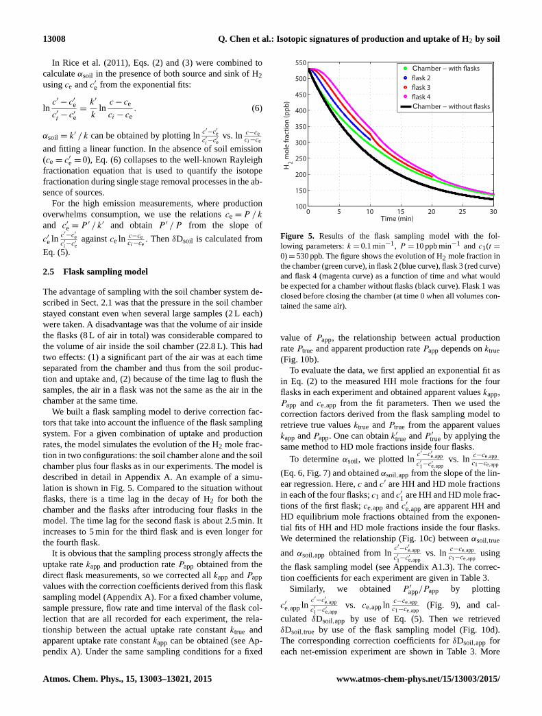
lation is shown in Fig. 5. Compared to the situation without

flasks, there is a time lag in the decay of H2 for both the

chamber and the flasks after introducing four flasks in the

model. The time lag for the second flask is about 2.5 min. It

increases to 5 min for the third flask and is even longer for

the fourth flask.

It is obvious that the sampling process strongly affects the

uptake rate kapp and production rate Papp obtained from the

direct flask measurements, so we corrected all kapp and Papp

values with the correction coefficients derived from this flask

sampling model (Appendix A). For a fixed chamber volume,

sample pressure, flow rate and time interval of the flask col-

lection that are all recorded for each experiment, the rela-

tionship between the actual uptake rate constant ktrue and

apparent uptake rate constant kapp can be obtained (see Ap-

pendix A). Under the same sampling conditions for a fixed

0 5 10 15 20 25 30100

150

200

250

300

350

400

450

500

550

Time (min)

H2 m

ole

frac

tion

(ppb

)

hamber − with �asks�ask 2�ask 3�ask 4

hamber − without �asks

C

C

Figure 5. Results of the flask sampling model with the fol-

lowing parameters: k = 0.1 min−1, P = 10 ppb min−1 and c1(t =

0)= 530 ppb. The figure shows the evolution of H2 mole fraction in

the chamber (green curve), in flask 2 (blue curve), flask 3 (red curve)

and flask 4 (magenta curve) as a function of time and what would

be expected for a chamber without flasks (black curve). Flask 1 was

closed before closing the chamber (at time 0 when all volumes con-

tained the same air).

value of Papp, the relationship between actual production

rate Ptrue and apparent production rate Papp depends on ktrue

(Fig. 10b).

To evaluate the data, we first applied an exponential fit as

in Eq. (2) to the measured HH mole fractions for the four

flasks in each experiment and obtained apparent values kapp,

Papp and ce,app from the fit parameters. Then we used the

correction factors derived from the flask sampling model to

retrieve true values ktrue and Ptrue from the apparent values

kapp and Papp. One can obtain k′true and P ′true by applying the

same method to HD mole fractions inside four flasks.

To determine αsoil, we plotted lnc′−c′e,app

c′1−c′e,app

vs. lnc−ce,app

c1−ce,app

(Eq. 6, Fig. 7) and obtained αsoil,app from the slope of the lin-

ear regression. Here, c and c′ are HH and HD mole fractions

in each of the four flasks; c1 and c′1 are HH and HD mole frac-

tions of the first flask; ce,app and c′e,app are apparent HH and

HD equilibrium mole fractions obtained from the exponen-

tial fits of HH and HD mole fractions inside the four flasks.

We determined the relationship (Fig. 10c) between αsoil,true

and αsoil,app obtained from lnc′−c′e,app

c′1−c′e,app

vs. lnc−ce,app

c1−ce,appusing

the flask sampling model (see Appendix A1.3). The correc-

tion coefficients for each experiment are given in Table 3.

Similarly, we obtained P ′app/Papp by plotting

c′e,app lnc′−c′e,app

c′1−c′e,app

vs. ce,app lnc−ce,app

c1−ce,app(Fig. 9), and cal-

culated δDsoil,app by use of Eq. (5). Then we retrieved

δDsoil,true by use of the flask sampling model (Fig. 10d).

The corresponding correction coefficients for δDsoil,app for

each net-emission experiment are shown in Table 3. More



Figure 6. Time evolution of H2, HD and δD in Cabauw (upper and middle panels) and in Speuld (lower panel) for representative experiments.

HD is calculated from H2 and δD. The H2 data are fitted with an exponential function of the form c =(c1− ce,app

)e−kappt + ce,app, where

c1 and ce,app are the H2 mole fractions initially and in equilibrium, and kapp is the apparent soil uptake rate constant for H2. A similar

exponential function is applied to the HD data. Error estimates for H2, HD and δD are shown. The connecting lines for δD data are included

to guide the eye.

information about the retrievals of αsoil,true and δDsoil,true

can be found in Appendix A.

Overall, the sampling effect on δDsoil is small (less than

22 ‰). This means that the flask sampling system strongly

affects the temporal evolution of HH and HD individually

(Fig. 5), and the uptake and production rates derived from

flask measurements, but the effects on the computed isotopic

signature of the source and sink are relatively small. More de-

tails and discussion of the flask sampling model corrections

are provided in Appendix A.

3 Results

3.1 Temporal evolution of H2, HD and δD

Figure 6 shows examples for the temporal evolution of H2,

HD and δD in Cabauw and Speuld, with error estimates in-



−8 −6 −4 −2 0−8

−6

−4

−2

0

ln[(c−ce,app

)/(c1

−ce,app

)]

ln[(c

’ −c’ e,

app)/

(c’ 1−c

’ e,ap

p)]

SPUCBWOverall �t

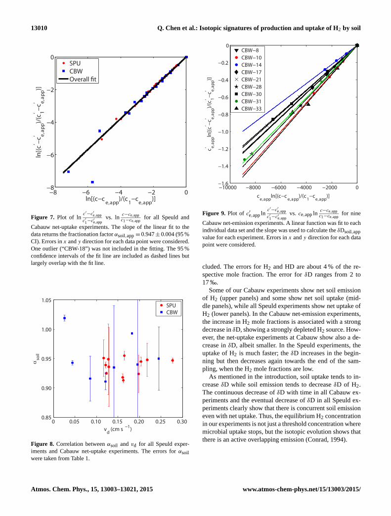
Figure 7. Plot of lnc′−c′e,app

c′1−c′e,app

vs. lnc−ce,app

c1−ce,appfor all Speuld and

Cabauw net-uptake experiments. The slope of the linear fit to the

data returns the fractionation factor αsoil,app = 0.947± 0.004 (95 %

CI). Errors in x and y direction for each data point were considered.

One outlier (“CBW-18”) was not included in the fitting. The 95 %

confidence intervals of the fit line are included as dashed lines but

largely overlap with the fit line.

0 0.05 0.10 0.15 0.20 0.25 0.300.85

0.90

0.95

1.00

1.05

vd

(cm s −1)

αso

il

SPUCBW

Figure 8. Correlation between αsoil and vd for all Speuld exper-

iments and Cabauw net-uptake experiments. The errors for αsoil

were taken from Table 1.

−10000 −8000 −6000 −4000 −2000 0−1.6

−1.4

−1.2

−1.0

−0.8

−0.6

−0.4

−0.2

0

ce,app

ln[(c−ce,app

)/(c1

−ce,app

)]

c’ e,ap

pln[(c

’ −c’ e,

app)/

(c’ 1−c

’ e,ap

p)]

CBW−8CBW−10CBW−14CBW−17CBW−21CBW−28CBW−30CBW−31CBW−33

Figure 9. Plot of c′e,app lnc′−c′e,app

c′1−c′e,app


c1−ce,appfor nine

Cabauw net-emission experiments. A linear function was fit to each

individual data set and the slope was used to calculate the δDsoil,app

value for each experiment. Errors in x and y direction for each data

point were considered.

cluded. The errors for H2 and HD are about 4 % of the re-

spective mole fraction. The error for δD ranges from 2 to

17 ‰.

Some of our Cabauw experiments show net soil emission

of H2 (upper panels) and some show net soil uptake (mid-

dle panels), while all Speuld experiments show net uptake of

H2 (lower panels). In the Cabauw net-emission experiments,

the increase in H2 mole fractions is associated with a strong

decrease in δD, showing a strongly depleted H2 source. How-

ever, the net-uptake experiments at Cabauw show also a de-

crease in δD, albeit smaller. In the Speuld experiments, the

uptake of H2 is much faster; the δD increases in the begin-

ning but then decreases again towards the end of the sam-

pling, when the H2 mole fractions are low.

As mentioned in the introduction, soil uptake tends to in-

crease δD while soil emission tends to decrease δD of H2.

The continuous decrease of δD with time in all Cabauw ex-

periments and the eventual decrease of δD in all Speuld ex-

periments clearly show that there is concurrent soil emission

even with net uptake. Thus, the equilibrium H2 concentration

in our experiments is not just a threshold concentration where

microbial uptake stops, but the isotopic evolution shows that

there is an active overlapping emission (Conrad, 1994).



Table 1. The deposition velocity (vd), fractionation factor (αsoil) as well as its error estimate and soil cover information for each Speuld

experiment (a) and Cabauw net-uptake experiment (b). The SD represents standard deviation and SE represents standard error. The errors of

αsoil represent the 95 % confidence interval (CI) for αsoil,app obtained from lnc′−c′e,app

c′1−c′e,app

vs. lnc−ce,app

c1−ce,app.

(a) Fn (nmol m−2 s−1) vd (cm s−1) αsoil Error αsoil Soil cover

SPU-1 −30.1 0.20 0.924 0.032 D. fir, moss

SPU-2 −35.3 0.22 0.948 0.028 D. fir, needles

SPU-3 −37.7 0.20 0.945 0.008 D. fir, moss

SPU-4 −26.1 0.16 0.913 0.004 D. fir, moss

SPU-5 −24.9 0.16 0.918 0.006 D. fir, moss

SPU-6 −13.2 0.12 0.951 0.031 D. fir, moss

SPU-7 −19.6 0.12 0.939 0.005 beech, leaves

SPU-8 −28.4 0.16 0.955 0.008 same subsite as SPU-7, leaves removed

SPU-9 −20.4 0.12 0.925 0.002 beech, leaves

SPU-10 −22.3 0.13 0.949 0.060 spruce, moss

SPU-11 −19.4 0.13 0.936 0.068 spruce, needles

SPU-12 −40.5 0.28 0.947 0.004 same subsite as SPU-11, needles removed

MEAN −26.5 0.17 0.937 – –

SD 8.2 0.05 0.014 – –

SE 2.4 0.01 0.004 – –

(b) Fn vd αsoil Error αsoil Soil cover

(nmol m−2 s−1) (cm s−1)

CBW-5 −6.6 0.04 0.943 0.004 few clover, grass

CBW-7 −3.1 0.03 1.019 0.005 few clover, grass

CBW-16 −22.9 0.18 0.993 0.001 bare soil, few grass

CBW-18 −39.3 0.24 0.950 0.054 grass

CBW-19 −7.4 0.14 0.935 0.105 grass

CBW-20 −14.9 0.20 0.940 0.260 bare soil

CBW-25 −8.0 0.12 0.911 0.014 clover, grass

CBW-26 −6.1 0.09 0.916 0.038 grass

MEAN −13.6 0.13 0.951 – –

SD 12.2 0.08 0.037 – –

SE 4.3 0.03 0.013 – –

3.2 Emission and uptake strength of H2

The production rate P = Ptrue and uptake rate constant

k = ktrue were obtained by applying exponential fits to the

temporal evolution of H2 and applying the corrections de-

rived from the flask sampling model (Appendix A) to the

Papp and kapp obtained from the exponential fits (Fig. 6). The

deposition velocity (vd), production flux (Fp), initial uptake

flux (Fu) and net flux at the beginning of the experiment (Fn)

were then calculated as follows:

vd = kh, (7)

Fp =Ph

VM

, (8)

Fu =kc1h

VM

, (9)

Fn = Fp−Fu, (10)

where h, VM and c1 are the chamber height, standard molar

volume (= 22.4 L mol−1) and H2 mole fraction of the first

flask, respectively. We note that with our method we derive

vd as deposition velocity for the gross uptake, unlike most

of the results reported in the literature that just measured net

uptake.

The strongest soil uptake occurs in the Speuld experi-

ments (Table 1a), with a mean vd of (0.17± 0.02) (2 SE,

n= 12) cm s−1 (SE represents standard error). On average,

the Cabauw experiments show weaker soil uptake, with

a mean vd of (0.13± 0.06) (2 SE, n= 8) cm s−1 for the

net-uptake experiments (Table 1b) and (0.06± 0.03) (2 SE,

n= 9) cm s−1 for the net-emission experiments (Table 2).

In terms of the net H2 flux Fn, this is (−26.5± 4.8) (2 SE,

n= 12) nmol m−2 s−1 for Speuld experiments (Table 1a),

(−13.6± 8.6) (2 SE, n= 8) nmol m−2 s−1 for Cabauw net-

uptake experiments (Table 1b) and (49.5± 29.8) (2 SE,

n= 9) nmol m−2 s−1 for Cabauw net-emission experiments



0 0.05 0.10 0.15 0.20 0.25 0.301.40

1.45

1.50

1.55

1.60

1.65

kapp

(min −1)

k true/k

app

Ptrue

=50 ppb min −1

Ptrue

=200 ppb min −1

Ptrue

=650 ppb min −1

0 50 100 150 200 250 300 350 400 4501.40

1.45

1.50

1.55

1.60

Papp

(ppb min −1)

Ptru

e/Pap

p

ktrue

=0.05 min −1

ktrue

=0.25 min −1

ktrue

=0.45 min −1

0.90 0.92 0.94 0.96 0.98 1.000.98

0.99

1.00

αsoil,app

αso

il,tr

ue/α

soil,

app

(δDsoil,true

+1)=0.25

(δDsoil,true

+1)=0.45

(δDsoil,true

+1)=0.65

0.25 0.3 0.35 0.4 0.45 0.5 0.55 0.6 0.650.99

1.00

1.01

1.02

1.03

1.04

1.05

(δDapp

+1)

(δD

true+1

)/(δ

Dap

p+1)

α

soil,true=0.90

αsoil,true

=0.95

αsoil,true

=1.00

(a) (b)

(d)(c)

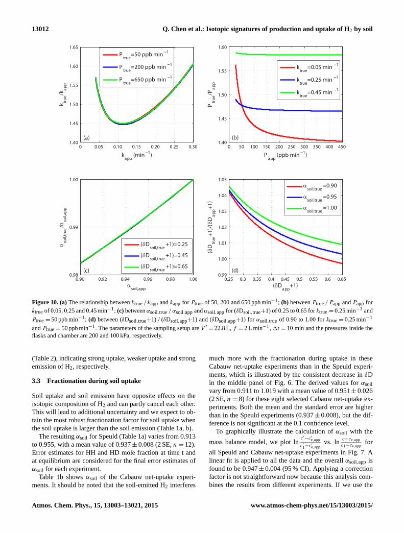
Figure 10. (a) The relationship between ktrue / kapp and kapp for Ptrue of 50, 200 and 650 ppb min−1; (b) between Ptrue / Papp and Papp for

ktrue of 0.05, 0.25 and 0.45 min−1; (c) between αsoil,true / αsoil,app and αsoil,app for (δDsoil,true+1) of 0.25 to 0.65 for ktrue = 0.25 min−1 and

Ptrue = 50 ppb min−1; (d) between (δDsoil,true+1) / (δDsoil,app+1) and (δDsoil,app+1) for αsoil,true of 0.90 to 1.00 for ktrue = 0.25 min−1

and Ptrue = 50 ppb min−1. The parameters of the sampling setup are V ′ = 22.8 L, f = 2 L min−1, 1t = 10 min and the pressures inside the

flasks and chamber are 200 and 100 kPa, respectively.

(Table 2), indicating strong uptake, weaker uptake and strong

emission of H2, respectively.

3.3 Fractionation during soil uptake

Soil uptake and soil emission have opposite effects on the

isotopic composition of H2 and can partly cancel each other.

This will lead to additional uncertainty and we expect to ob-

tain the most robust fractionation factor for soil uptake when

the soil uptake is larger than the soil emission (Table 1a, b).

The resulting αsoil for Speuld (Table 1a) varies from 0.913

to 0.955, with a mean value of 0.937± 0.008 (2 SE, n= 12).

Error estimates for HH and HD mole fraction at time t and

at equilibrium are considered for the final error estimates of

αsoil for each experiment.

Table 1b shows αsoil of the Cabauw net-uptake experi-

ments. It should be noted that the soil-emitted H2 interferes

much more with the fractionation during uptake in these

Cabauw net-uptake experiments than in the Speuld experi-

ments, which is illustrated by the consistent decrease in δD

in the middle panel of Fig. 6. The derived values for αsoil

vary from 0.911 to 1.019 with a mean value of 0.951± 0.026

(2 SE, n= 8) for these eight selected Cabauw net-uptake ex-

periments. Both the mean and the standard error are higher

than in the Speuld experiments (0.937± 0.008), but the dif-

ference is not significant at the 0.1 confidence level.

To graphically illustrate the calculation of αsoil with the

mass balance model, we plot lnc′−c′e,app

c′1−c′e,app

vs. lnc−ce,app

c1−ce,appfor

all Speuld and Cabauw net-uptake experiments in Fig. 7. A

linear fit is applied to all the data and the overall αsoil,app is

found to be 0.947± 0.004 (95 % CI). Applying a correction

factor is not straightforward now because this analysis com-

bines the results from different experiments. If we use the



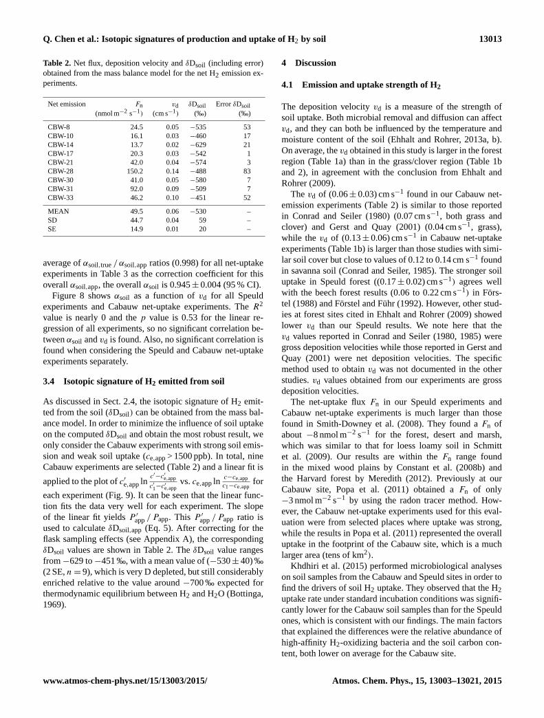
Table 2. Net flux, deposition velocity and δDsoil (including error)

obtained from the mass balance model for the net H2 emission ex-

periments.

Net emission Fn vd δDsoil Error δDsoil

(nmol m−2 s−1) (cm s−1) (‰) (‰)

CBW-8 24.5 0.05 −535 53

CBW-10 16.1 0.03 −460 17

CBW-14 13.7 0.02 −629 21

CBW-17 20.3 0.03 −542 1

CBW-21 42.0 0.04 −574 3

CBW-28 150.2 0.14 −488 83

CBW-30 41.0 0.05 −580 7

CBW-31 92.0 0.09 −509 7

CBW-33 46.2 0.10 −451 52

MEAN 49.5 0.06 −530 –

SD 44.7 0.04 59 –

SE 14.9 0.01 20 –

average of αsoil,true / αsoil,app ratios (0.998) for all net-uptake

experiments in Table 3 as the correction coefficient for this

overall αsoil,app, the overall αsoil is 0.945± 0.004 (95 % CI).

Figure 8 shows αsoil as a function of vd for all Speuld

experiments and Cabauw net-uptake experiments. The R2

value is nearly 0 and the p value is 0.53 for the linear re-

gression of all experiments, so no significant correlation be-

tween αsoil and vd is found. Also, no significant correlation is

found when considering the Speuld and Cabauw net-uptake

experiments separately.

3.4 Isotopic signature of H2 emitted from soil

As discussed in Sect. 2.4, the isotopic signature of H2 emit-

ted from the soil (δDsoil) can be obtained from the mass bal-

ance model. In order to minimize the influence of soil uptake

on the computed δDsoil and obtain the most robust result, we

only consider the Cabauw experiments with strong soil emis-

sion and weak soil uptake (ce,app > 1500 ppb). In total, nine

Cabauw experiments are selected (Table 2) and a linear fit is

applied to the plot of c′e,app lnc′−c′e,app

c′1−c′e,app


c1−ce,appfor

each experiment (Fig. 9). It can be seen that the linear func-

tion fits the data very well for each experiment. The slope

of the linear fit yields P ′app / Papp. This P ′app / Papp ratio is

used to calculate δDsoil,app (Eq. 5). After correcting for the

flask sampling effects (see Appendix A), the corresponding

δDsoil values are shown in Table 2. The δDsoil value ranges

from−629 to−451 ‰, with a mean value of (−530± 40) ‰

(2 SE, n= 9), which is very D depleted, but still considerably

enriched relative to the value around −700 ‰ expected for

thermodynamic equilibrium between H2 and H2O (Bottinga,

1969).

4 Discussion

4.1 Emission and uptake strength of H2

The deposition velocity vd is a measure of the strength of

soil uptake. Both microbial removal and diffusion can affect

vd, and they can both be influenced by the temperature and

moisture content of the soil (Ehhalt and Rohrer, 2013a, b).

On average, the vd obtained in this study is larger in the forest

region (Table 1a) than in the grass/clover region (Table 1b

and 2), in agreement with the conclusion from Ehhalt and

Rohrer (2009).

The vd of (0.06± 0.03) cm s−1 found in our Cabauw net-

emission experiments (Table 2) is similar to those reported

in Conrad and Seiler (1980) (0.07 cm s−1, both grass and

clover) and Gerst and Quay (2001) (0.04 cm s−1, grass),

while the vd of (0.13± 0.06) cm s−1 in Cabauw net-uptake

experiments (Table 1b) is larger than those studies with simi-

lar soil cover but close to values of 0.12 to 0.14 cm s−1 found

in savanna soil (Conrad and Seiler, 1985). The stronger soil

uptake in Speuld forest ((0.17± 0.02) cm s−1) agrees well

with the beech forest results (0.06 to 0.22 cm s−1) in Förs-

tel (1988) and Förstel and Führ (1992). However, other stud-

ies at forest sites cited in Ehhalt and Rohrer (2009) showed

lower vd than our Speuld results. We note here that the

vd values reported in Conrad and Seiler (1980, 1985) were

gross deposition velocities while those reported in Gerst and

Quay (2001) were net deposition velocities. The specific

method used to obtain vd was not documented in the other

studies. vd values obtained from our experiments are gross

deposition velocities.

The net-uptake flux Fn in our Speuld experiments and

Cabauw net-uptake experiments is much larger than those

found in Smith-Downey et al. (2008). They found a Fn of

about −8 nmol m−2 s−1 for the forest, desert and marsh,

which was similar to that for loess loamy soil in Schmitt

et al. (2009). Our results are within the Fn range found

in the mixed wood plains by Constant et al. (2008b) and

the Harvard forest by Meredith (2012). Previously at our

Cabauw site, Popa et al. (2011) obtained a Fn of only

−3 nmol m−2 s−1 by using the radon tracer method. How-

ever, the Cabauw net-uptake experiments used for this eval-

uation were from selected places where uptake was strong,

while the results in Popa et al. (2011) represented the overall

uptake in the footprint of the Cabauw site, which is a much

larger area (tens of km2).

Khdhiri et al. (2015) performed microbiological analyses

on soil samples from the Cabauw and Speuld sites in order to

find the drivers of soil H2 uptake. They observed that the H2

uptake rate under standard incubation conditions was signifi-

cantly lower for the Cabauw soil samples than for the Speuld

ones, which is consistent with our findings. The main factors

that explained the differences were the relative abundance of

high-affinity H2-oxidizing bacteria and the soil carbon con-

tent, both lower on average for the Cabauw site.



Table 3. Sampling information and the correction coefficients (ktrue / kapp, Ptrue / Papp, αsoil,true / αsoil,app and (δDsoil,true+1) /

(δDsoil,app+1) used for each experiment. Size S refers to small chamber and size L refers to large chamber.

Exp. Pressure Flow rate Size 1t kapp Papp ktrue / kapp Ptrue / Papp αsoil,true/αsoil,app (δDsoil,true+1)/

(kPa) (L min−1) (min) (min−1) (ppb min−1) (δDsoil,app+1)

SPU-1 200 2 S 10 0.199 4.12 1.494 1.601 0.984 –

SPU-2 200 2.2 S 5 0.206 0.67 1.589 7.472 0.998 –

SPU-3 200 3.1 S 5 0.204 3.58 1.496 2.475 0.999 –

SPU-4 200 2.8 S 5 0.160 7.51 1.526 2.136 1.004 –

SPU-5 200 2.6 S 5 0.156 4.16 1.546 2.759 1.004 –

SPU-6 160 3.2 L 5 0.232 7.61 1.184 1.446 0.999 –

SPU-7 160 3.2 S 5 0.128 5.40 1.418 2.264 1.006 –

SPU-8 160 2.5 S 5 0.172 4.23 1.438 2.381 1.001 –

SPU-9 160 2.8 S 5 0.128 4.56 1.440 2.513 1.007 –

SPU-10 180 2.7 S 5 0.128 – 1.502 / 1.005 –

SPU-11 160 2.2 S 5 0.130 – 1.490 / 1.006 –

SPU-12 180 2.3 S 5 0.272 11.30 1.529 1.720 0.994 –

CBW-5 200 2 L 10 0.086 18.24 1.204 1.248 1.001 –

CBW-7 200 1.9 L 10 0.048 11.57 1.260 1.361 0.999 –

CBW-16 210 2.1 S 10 0.183 45.21 1.498 1.505 0.999 –

CBW-18 200 2 S 10 0.240 38.07 1.532 1.527 0.986 –

CBW-19 200 2 S 10 0.145 56.69 1.457 1.463 0.991 –

CBW-20 200 2 S 10 0.196 65.81 1.491 1.494 0.988 –

CBW-25 200 2 S 10 0.122 44.85 1.449 1.460 0.994 –

CBW-26 200 2 S 10 0.088 31.05 1.452 1.475 1.002 –

CBW-8 200 2 S 10 0.044 82.92 1.542 1.438 – 1.048

CBW-10 200 2.6 L 10 0.069 111.00 1.177 1.152 – 1.010

CBW-14 200 2.5 L 10 0.035 82.53 1.251 1.166 – 1.042

CBW-17 220 2.1 L 10 0.047 117.40 1.268 1.198 – 1.024

CBW-21 220 2 L 10 0.078 232.20 1.209 1.179 – 1.008

CBW-28 175 1.8 S 10 0.146 440.90 1.412 1.402 – 1.018

CBW-30 200 2 L 10 0.090 237.70 1.202 1.180 – 1.008

CBW-31 200 2 S 10 0.098 275.10 1.451 1.422 – 1.007

CBW-33 200 2 S 10 0.107 166.50 1.449 1.430 – 1.007

The emission of H2 from the soil is large for the

Cabauw net-emission experiments, with Fn ranging from

13.7 to 150.2 nmol m−2 s−1 and a median value of

41.0 nmol m−2 s−1 (Table 2). One experiment, “CBW-28”,

shows unusually high emission, with H2 increasing to 3010

ppb within 30 min. In comparison, Conrad and Seiler (1980)

found a Fn of 23–32 nmol m−2 s−1 for a clover field. Except

for the experiments “CBW-28” and “CBW-31”, our Cabauw

net-emission experiments are close to the Fn found by them.

The variability in Fn could be attributed to different N2 fixa-

tion flux in our experiments, which could be affected by both

spatial density of N2 fixation organisms and their N2 fixation

activities. The N2 fixation activity could be regulated by vari-

ous factors including temperature, moisture, light availability

and carbon storage (Belnap, 2001), which were not measured

are therefore not discussed here.

4.2 Fractionation during soil uptake

Fractionation during soil uptake of H2 can happen during the

diffusion into the soil and due to microbial removal within

the soil. To further investigate the factors determining αsoil,

information about the soil cover is provided in Table 1a, b. It

is evident that no large differences exist between the Douglas

fir, spruce and beech sites, i.e., the variability between sites

is similar to the variability within sites. The small number

of experiments impedes examining the possible small dif-

ferences between sites. In order to investigate the diffusion

effect, we removed the soil cover in experiments “SPU-8”

and “SPU-12” at the same place of experiments “SPU-7”

and “SPU-11”. The removal of leaves (“SPU-8”) and needles

(“SPU-12”) increased αsoil by ≈ 0.014, thus towards smaller

fractionation, which indicates that diffusion contributes to

the fractionation. As vd also increases when the soil cover

is removed, faster deposition is associated with smaller frac-

tionations in these experiments, which is similar to the results

from Rice et al. (2011).

The αsoil for the Cabauw net-uptake experiments is higher

and more scattered than that for the Speuld experiments

(0.951± 0.026 vs. 0.937± 0.008). This could be caused by

the interference of D-depleted H2 from the strong soil emis-

sion in Cabauw, which may not be perfectly captured via the

mathematical models applied. As can be seen from the strong

decline of δD with time in the middle panel of Fig. 6, though

soil uptake of H2 dominates for the Cabauw net-uptake ex-

periments, soil production is still considerable. If part of the



source signature is not taken into account properly and ap-

pears in αsoil, then αsoil will be larger, because soil produc-

tion tends to decrease δD of H2. This could explain why αsoil

is even larger than 1 in “CBW-7”.

The overall αsoil (0.945) obtained by plotting lnc′−c′e,app

c′1−c′e,app

vs. lnc−ce,app

c1−ce,appand applying the average correction factor for

all the Speuld and Cabauw net-uptake experiments is similar

to the results of 0.943± 0.024 from Gerst and Quay (2001),

0.94± 0.01 from Rahn et al. (2002a), and the overall αsoil

(0.943) from Rice et al. (2011). Rice et al. (2011) suggested

that the overall αsoil is more accurate as it is less susceptible

to outliers. We argue here that the average αsoil of all indi-

vidual experiments in Speuld (0.937) and Cabauw (0.951)

is representative for a spatially averaged fractionation fac-

tor for those sites and is useful for, e.g., characterizing the

phenomenon and comparing with other fractionation results.

If all experiments are included in one fit, their weight for

determining the slopes depends on how much H2 has been

removed, so experiments with a lower ce,app have a larger

weight than experiments with a higher ce,app (i.e., experi-

ments with a higher vd have a larger weight than experi-

ments with a lower vd). The fractionation factor obtained by

fitting all data together is therefore representative for a flux

weighted average, which is the relevant number for the global

atmospheric isotope budget.

4.3 Relationship between αsoil and vd

Rice et al. (2011) proposed a significant positive correlation

between αsoil and deposition velocity vd in their soil uptake

experiments. Figure 8 shows that no significant correlation

between αsoil and vd is found when considering all Speuld

and Cabauw net-uptake experiments. The uptake rate is much

stronger in the Speuld experiments (vd ≈ 0.17 cm s−1) than

in the study of Rice et al. (2011) (vd ≈ 0.04 cm s−1), but the

αsoil is virtually identical (0.937 vs. 0.934). Therefore, when

the results from both studies are combined, the correlation re-

ported in Rice et al. (2011) between αsoil and vd disappears.

We suggest that a positive correlation between αsoil and vd

may exist for a specific site where microbial species are sim-

ilar. This was suggested from the simultaneous increase of

both αsoil and vd in two experiments (“SPU-8” and “SPU-

12”), when soil cover was removed at the same sampling lo-

cation, as mentioned in Sect. 4.2.

We conclude that there is certainly not one single correla-

tion between αsoil and vd that holds globally and the soil type

might play an important role. Measurements at more sites

may be needed to positively confirm whether local positive

correlations between αsoil and vd are common.

4.4 δD of H2 emitted from the soil

The present study is the first field study to report δD of H2

emitted from soils. The δDsoil values (−629 to −451 ‰)

shown in Table 2 are less depleted than the H2 in isotopic

equilibrium with water (≈−700 ‰). Previous observations

from environmental H2 production yielded a δD of −628 ‰

for two seawater samples (Rice et al., 2010), −778 ‰ for

a termite headspace sample and −690 ‰ for two headspace

samples from a eutrophic water pond (Rahn et al., 2002b).

Kawagucci et al. (2010) proposed that microbiological H2

consumption and production could destroy the thermal iso-

topic equilibrium between H2 and H2O in low-temperature

hydrothermal fluids. Luo et al. (1991) and Walter et al. (2012)

found fractionation factors of 0.448, 0.401 and 0.363 for H2

generated from water by different N2-fixing bacteria in the

laboratory.

In order to compare our δDsoil with the fractionation fac-

tors between H2 and H2O found by Luo et al. (1991) and

Walter et al. (2012), we converted their fractionation factors

to δD(H2) by assuming the δD(H2O) to be the same as that

of global rainwater (−37.8 ‰, Hoffmann et al., 1998). This

results in δD(H2) values of −651 to −569 ‰ for their N2-

fixing bacteria. Although the ranges are considerable, it ap-

pears that the mean δDsoil (−530 ‰) obtained in our field

study is even higher than what was found for nitrogenase-

derived H2 in laboratory experiments.

It is known that H2 produced by biogenic N2 fixation can

be largely recycled within the soil before entering the atmo-

sphere (Evans et al., 1987; Conrad and Seiler, 1979, 1980). If

this uptake process within the soil tends to increase the δD of

the remaining H2, as the soil uptake process for atmospheric

H2 does, then the H2 entering the atmosphere will be less D

depleted than pure biogenic H2. However, if the fractionation

factor of removal in the soil is similar to that determined from

the net-uptake experiments (≈ 0.94), a large fraction (fin) of

H2 needs to be removed in the soil before release to explain

the D-enriched δDsoil compared to the values reported in the

literature. The fraction fin could in principle be estimated

from the Rayleigh equation:

(1− fin)αin−1=δDsoil+ 1

δD0+ 1,

where αin is the fractionation constant of H2 within soil,

δD0 is the δD value of initial H2 produced by N2-fixers,

and δDsoil is the δD value of remaining H2 emitted from

soil that is measured in our experiments. By assuming

αin = 0.945 (overall fractionation factor as determined in our

deposition experiments), δDsoil =−530 ‰ (averaged δDsoil

of Cabauw net-emission experiments) and δD0 =−611 ‰

(averaged of δD(H2) derived from laboratory experiments

in Luo et al. (1991) and Walter et al., 2012), we would ob-

tain fin = 0.97. That is, 97 % of H2 produced by N2 fix-

ation would be removed within soil before entering atmo-

sphere. This is higher than the estimate from Conrad and

Seiler (1979), which was from 30 to 90 %. It should be noted

that the estimation of fin is very uncertain due to the lack

of information about αin and δD0. By using the lower limit

of αin (0.911) in our experiment and the upper limit of δD0



(−569 ‰) in Luo et al. (1991) and Walter et al. (2012), we

calculate a lower limit of fin to be 0.62. The upper limit of

fin is 1.00 when αin approaches 1. For these calculations we

have used a δDsoil of −530 ‰ , but it varies from −629 to

−451 ‰ in our experiments. We cannot rule out cases with

δDsoil = δD0, which yields a fin of 0.

The deuterium enrichment in the emitted H2, compared to

the value expected in isotopic equilibrium with water, could

also be caused by different fractionations induced by differ-

ent enzymes and/or a potentially enriched deuterium content

of the substrate water available for H2 production in Cabauw.

H2 is generated from the reduction of hydrogen ions (H+ or

D+) in intracellular water (Yang et al., 2012). It was found

that the isotopic composition of intracellular water can be

different from that of extracellular water due to metabolic

processing (Kreuzer-Martin et al., 2006). Due to the differ-

ences in H bonding and hydrogen ion transport, the fraction-

ation may be different for different microbe species, which

could result in different isotopic signatures of the produced

H2. Measurements of the isotopic composition of produced

H2 may be a tool to investigate such effects.

Finally, we note that if our Cabauw net-emission experi-

ments are analyzed with a simple Keeling plot approach (i.e.,

without considering uptake), the y axis intercept is −703 ‰.

We know from the temporal evolution of H2, HD and δD that

this model is not adequate and that uptake was significant in

our experiments, so a simple Keeling plot analysis can be

misleading if uptake is not considered.

5 Conclusions

This study investigated the isotope effects associated with the

production and uptake of atmospheric H2 by soil. Our aim

was to quantify the fractionation factor αsoil for H2 deposi-

tion and the isotopic signature of H2 emitted from the soil

(δDsoil) from experiments carried out at Speuld and Cabauw.

The experiments covered a wide range of conditions from

situations with very strong net H2 uptake to situations with

very strong net H2 emission. The superposition of deposi-

tion and production made the analysis with simple models

like Rayleigh plot and Keeling plot impossible. Therefore,

the mass balance model suggested by Rice et al. (2011) was

used for evaluation.

The deposition velocity vd was largest in the Speuld ex-

periments ((0.17± 0.02) cm s−1) where also the strongest

net soil uptake occurred, followed by the Cabauw net-

uptake experiments ((0.13± 0.06) cm s−1) and Cabauw net-

emission experiments ((0.06± 0.03) cm s−1). The net H2

flux Fn was (−26.5± 4.8) nmol m−2 s−1 for Speuld exper-

iments, (−13.6± 8.6) nmol m−2 s−1 for Cabauw net-uptake

experiments and (49.5± 29.8) nmol m−2 s−1 for Cabauw

net-emission experiments.

The mean fractionation factors αsoil are 0.937± 0.008 for

the Speuld forest soil experiments and 0.951± 0.026 for the

Cabauw grassland experiments, which are representative for

a spatial average and useful for comparisons with other frac-

tionation studies. The Cabauw results may be affected by the

relatively strong concomitant soil emissions. The overall αsoil

by considering all net-uptake experiments is 0.945± 0.004,

which is representative for a flux weighted average and use-

ful for global isotope budget estimates. The fractionation fac-

tors found in this work are in good agreement with previous

studies.

No significant correlation between αsoil and deposition ve-

locity vd was found while considering all of our experiments.

The vd were overall much larger in our study than those in

Rice et al. (2011) and we obtained similar values for αsoil.

This demonstrates that the positive correlation that was found

previously does not hold globally. From two of our Speuld

experiments, αsoil increased after the removal of leaves or

needles above the soil. This indicates that there may be a

fractionation associated with diffusion through the surface

layer of leaves or needles during soil uptake, but more exper-

iments are required to confirm this.

The isotopic analysis clearly showed that the net uptake

was always a superposition of a larger gross uptake and a

gross emission flux. In Cabauw, the emission strength was

very large at locations where clover was present. Using a

simple mass balance approach, the isotopic composition of

the emitted H2 was determined to be (−530± 40) ‰, which

is significantly higher than the value expected for H2O–H2

isotope equilibrium. Although limited, other published data

on H2 produced biologically via nitrogenase show also a ten-

dency to more enriched values. An additional isotope enrich-

ment in our field soil study could originate from fractionation

during the recycling of H2 within the soil before it enters the

atmosphere.



Appendix A

A1 Flask sampling model

A mathematical model is used to simulate the sampling and

to correct for the effects of the flask sampling method on the

values of uptake rate constant (k), production rate (P ), frac-

tionation factor (αsoil) and isotopic signature of H2 produced

from soil (δDsoil). We start with a pair of known (true) uptake

and production rates and simulate the evolution of the mole

fractions of H2 and HD in the flasks and chamber. From the

modeled mole fractions we calculate the apparent uptake and

production rates and derive the correction needed to obtain

the true uptake and production rates from measurement of

the apparent rates in actual experiments.

A1.1 Mathematical description of the flask sampling

model

The sampling setup is shown in Fig. 2 of the main paper.

After 10 min of flushing, the chamber and the flasks con-

tain ambient air with the prevailing H2 and HD mole frac-

tions. In the following we denote c1(t), c2(t), c3(t), c4(t)

and c0(t) the H2 mole fractions for the first, second, third

and fourth flask and the chamber, respectively. The moment

when the first flask and the chamber lid are closed is con-

sidered the starting time of the experiment (t = 0). From this

point on, only the chamber and the second, third and fourth

flask are connected, and the initial H2 mole fraction inside

them is c0(0) = c2(0)= c3(0)= c4(0)= c1. We start a simu-

lation with an input uptake rate constant (ktrue) and an input

production rate (Ptrue). The simulation of the flask sampling

is based on Eqs. (A1)–(A4) shown below.

Assuming that the air in each flask and in the chamber is

well mixed during the entire sampling process, the time evo-

lution for the second flask c2(t), third flask c3(t), fourth flask

c4(t) and the chamber c0(t) in the first 10 min after starting

the experiment can be expressed as

dc2(t)

dt=f

Vc0(t)−

f

Vc2(t), (A1)

dc3(t)

dt=f

Vc2(t)−

f

Vc3(t), (A2)

dc4(t)

dt=f

Vc3(t)−

f

Vc4(t), (A3)

dc0(t)

dt=f

V ′c4(t)−

f

V ′c0(t)+ (Ptrue− ktruec0(t)), (A4)

where V and V ′ are the air volumes of the flask and chamber,

and f is the flow rate. These differential equations are solved

using the Matlab ODE solvers at time steps of 0.01 min. The

input parameters are c0(0), Ptrue, ktrue, V , V ′ and f . For each

time step the solvers calculate the hydrogen flux into and out

of the chamber and each flask, as well as the new mole frac-

tions there.

After 10 min, the second flask is closed and now contains

air with mole fraction c2 = c2(10 min). From this point on,

only the chamber, the third and the fourth flask are con-

nected, and the time evolution of the mole fractions can be

expressed as

dc3(t)

dt=f

Vc0(t)−

f

Vc3(t), (A5)

dc4(t)

dt=f

Vc3(t)−

f

Vc4(t), (A6)

dc0(t)

dt=f

V ′c4(t)−

f

V ′c0(t)+ (Ptrue− ktruec0 (t)). (A7)

After another 10 min of sampling, the third flask is closed

c3 = c3(20 min), and only the chamber and the fourth flask

are connected. Then, the time evolution for the fourth flask

and the chamber can be expressed as

dc4(t)

dt=f

Vc0(t)−

f

Vc4(t), (A8)

dc0(t)

dt=f

V ′c4(t)−

f

V ′c0(t)+ (Ptrue− ktruec0(t)). (A9)

The H2 mole fraction inside the chamber and the fourth flask

at time t = 30 min is c0(30) and c4(30).

In the end, a set of four flasks with mole fractions c1(0),

c2(10 min), c3(20 min) and c4(30 min) is obtained. By fit-

ting this set of four data points with an exponential function

c = ae−kappt + ce,app (see Eq. 2 in the main paper), we can

obtain the apparent soil uptake rate constant (kapp) and equi-

librium concentration (ce,app) and further calculate apparent

production rate (Papp = kappce,app). These apparent rates kapp

and Papp are different from the assumed true rates ktrue and

Ptrue. The flask sampling model enables us to establish a re-

lation between kapp and Papp and ktrue and Ptrue, so that ktrue

and Ptrue can be derived from kapp and Papp in actual exper-

iments, where the true values are unknown. To accomplish

this, simulations are carried out with a wide range of values

for ktrue and Ptrue, and a corresponding data set of kapp and

Papp is generated. Similarly, we use a new set of input up-

take rate constant k′true and production rate P ′true for HD and

generate a corresponding data set of k′app and P ′app.

A1.2 The correction coefficients for k and P

Here we discuss an example of the relationship between ktrue

and kapp for the setup used in some Cabauw experiments

(V ′ = 22.8 L, f =2 L min−1 and1t = 10 min). The pressure

inside the flasks is 200 kPa and the pressure inside the cham-

ber is 100 kPa. The relationship between ktrue / kapp and kapp

is shown in Fig. 10a. The ratio ktrue / kapp varies between 1.45

to 1.61 for our kapp range of 0.04 to 0.30 min−1. This rela-

tionship does not depend on Ptrue (with Ptrue varying from 50

to 650 ppb min−1). An additional uncertainty can arise from

incorrect timing of the flask sampling, but sampling times

should be correct within few seconds, which may lead to an

additional uncertainty of below 1 %. The uncertainty of the



flow rate obtained from the rotameter due to variations in am-

bient pressure and temperature that were not recorded is less

than 4 %, and the effect on the ratio ktrue / kapp ratio is be-

low 1 %. We can retrieve ktrue by multiplying kapp with the

modeled value of ktrue / kapp for each experiment. The ratio

ktrue / kapp for each experiment is shown in Table 3. It de-

pends on experimental setup and kapp of each experiment,

with a range of 1.177 to 1.589.

After retrieving ktrue from kapp, we investigate the rela-

tionship between Ptrue / Papp and Papp for a fixed value of

ktrue (Fig. 10b). The ratio Ptrue/Papp depends slightly on Papp

and ktrue, ranging from 1.40 to 1.59 for a wide Papp range

of 30 to 450 ppb min−1 and a wide ktrue range of 0.05 to

0.45 min−1. As for the correction of k, uncertainties arising

from incorrect timing of the flask sampling and from pres-

sure and temperature variations and their effect on the flow

rate lead to additional uncertainties of Ptrue / Papp ratio be-

low 1 %, which are not considered. We can retrieve Ptrue by

multiplying Papp with Ptrue / Papp for each experiment after

having determined ktrue from kapp. The ratio Ptrue / Papp for

each experiment is shown in Table 3 and depends on the ex-

perimental setup, Papp and kapp of each experiment. It ranges

from 1.152 to 2.759 for most experiments, with an excep-

tion of 7.472 for experiment SPU-2 where a very small Papp

of 0.67 ppb min−1 is found. Although the ratio Ptrue / Papp of

experiment SPU-2 is high, Ptrue of SPU-2 is still smaller than

the rest of the experiments. Ptrue / Papp ratios for experiments

SPU-10 and SPU-11 are null because these two experiments

show a Papp of 0.

A1.3 The correction coefficients for αsoil and δDsoil

In our experiments, the uncertainties of kapp and k′app de-

rived from exponential fits to the time evolution of HH

and HD are rather large, which results in a large scatter of

αsoil,app if αsoil,app is calculated directly as k′app / kapp. Thus,

we obtained αsoil,app by plotting lnc′−c′e,app

c′1−c′e,app

vs. lnc−ce,app

c1−ce,app

(Fig. 7) for each experiment which yields a smaller scatter

for αsoil,app.

Correction coefficients to convert αsoil,app to αsoil,true

are obtained using the flask sampling model by compar-

ing αsoil,true used as input for the model run to αsoil,app

derived from the plot of lnc′−c′e,app

c′1−c′e,app

vs. lnc−ce,app

c1−ce,appof

the output values, like in the experiments. Figure 10c

shows αsoil,true / αsoil,app as a function of αsoil,app for

a wide δDsoil,true range of −750 to −250 ‰ with

the sampling setup described above (V ′ = 22.8 L,

f = 2 L min−1 and 1t = 10 min) for ktrue = 0.25 min−1

and Ptrue = 50 ppb min−1. In this case the correction

factor αsoil,true / αsoil,app varies from 0.98 to 1.00 for a

αsoil,app range of 0.90 to 1.00, and it does not depend on

δDsoil,true. Thus, after retrieving ktrue and Ptrue as described

in Sect. A1.2, we can retrieve αsoil,true from αsoil,app for

each experiment. The correction factors range from 0.984 to

1.007, depending on the experimental setup and αsoil,app of

each experiment (Table 3).

Similarly, in our experiments, the uncertainties of Papp

and P ′appderived from exponential fits of time evolution

of HH and HD are large, which results in a large scat-

ter of δDsoil,app if δDsoil,app is calculated directly from

these P ′app and Papp. We therefore obtained the ratio

P ′app / Papp by plotting c′e,app lnc′−c′e,app

c′1−c′e,app


c1−ce,app

(Fig. 9) and calculated δDsoil,app from Eq. (4). This yielded

smaller scatter for δDsoil,app. After retrieving ktrue, Ptrue

and αsoil,true as described above, we used the flask sam-

pling model again to derive correction factors by compar-

ing δDsoil,true used as model input with δDsoil,app obtained

from c′e,app lnc′−c′e,app

c′1−c′e,app


c1−ce,appof the model out-

put and to retrieve δDsoil,true from δDsoil,app for each ex-

periment. Figure 10d shows (δDsoil,true+1) / (δDsoil,app+1)

as a function of (δDsoil,app+1) for a αsoil,true range

of 0.90 to 1.00 with the sampling setup described

above (V ′ = 22.8 L, f =2 L min−1 and 1t = 10 min) for

ktrue = 0.25 min−1 and Ptrue = 50 ppb min−1. The ratio

(δDsoil,true+1) / (δDsoil,app+1) changes from 0.99 to 1.05 for

a wide (δDsoil,app+1) range of 0.25 to 0.65. It can be seen

that the (δDsoil,true+1) / (δDsoil,app+1) ratio depends slightly

on αsoil,true at a fixed (δDsoil,app+1), with a maximum differ-

ence of about 1 % for a αsoil,true range of 0.90 to 1.00. The ra-

tio (δDsoil,true+1) / (δDsoil,app+1) for each net-emission ex-

periment is shown in Table 3, ranging from 1.007 to 1.048.

The largest difference between δDsoil,true and δDsoil,app is

21 ‰ for CBW-8. The mean δDtrue and δDapp for these net-

emission experiments are −530 and −538 ‰, respectively.

In conclusion, the effect of the flask sampling process is

relatively small for αsoil and δDsoil but considerable for the

uptake rate constants k and k′ and emission rates P and P ′.

The flask sampling model allows us to derive corresponding

corrections that have been applied to correct for the bias in-

troduced by the flask sampling system.



Acknowledgements. We are grateful to C. Van der Veen, M. Bolder

and H. Snellen for their help maintaining the GC-IRMS system

and setup of the sampling. We are also grateful to Jan Kaiser

for giving valuable comments on the flask sampling model. This

work was supported by the Netherlands Organisation for Scientific

Research (NWO) as part of the NWO-ACTS Sustainable Hydrogen

(H2) project 2007/00566/ACTS, grant numbers 053.61.026 and

053.61.126.

Edited by: J. Kaiser

References

Batenburg, A. M., Walter, S., Pieterse, G., Levin, I., Schmidt, M.,

Jordan, A., Hammer, S., Yver, C., and Röckmann, T.: Temporal

and spatial variability of the stable isotopic composition of atmo-

spheric molecular hydrogen: observations at six EUROHYDROS

stations, Atmos. Chem. Phys., 11, 6985–6999, doi:10.5194/acp-

11-6985-2011, 2011.

Beljaars, A. C. M. and Bosveld, F. C.: Cabauw data

for the validation of land surface parameterization

schemes, J. Climate, 10, 1172–1193, doi:10.1175/1520-

0442(1997)010<1172:CDFTVO>2.0.CO;2, 1997.

Belnap, J.: Factors influencing nitrogen fixation and nitrogen re-

lease in biological soil crusts, Springer-Verlag, Berlin, Heidel-

berg, 241–261, 2001.

Bottinga, Y.: Calculated fractionation factors for carbon and

hydrogen isotope exchange in the system calcite-carbon

dioxide-graphite-methane-hydrogen-water vapour, Geochim.

Cosmochim. Ac., 33, 49–64, doi:10.1016/0016-7037(69)90092-

1, 1969.

Conrad, R.: Compensation concentration as critical variable for reg-

ulating the flux of trace gases between soil and atmosphere, Bio-

geochemistry, 27, 155–170, doi:10.1007/BF00000582, 1994.

Conrad, R. and Seiler W.: Field measurements of hydrogen evolu-

tion by nitrogen-fixing legumes, Soil Biol. Biochem., 11, 689–

690, doi:10.1016/0038-0717(79)90041-5, 1979.

Conrad, R. and Seiler, W.: Contribution of hydrogen production

by biological nitrogen fixation to the global hydrogen budget, J.

Geophys. Res., 85, 5493–5498, doi:10.1029/JC085iC10p05493,

1980.

Conrad, R. and Seiler, W.: Decomposition Of atmospheric hydrogen

by soil microorganisms and soil enzymes, Soil Biol. Biochem.,

13, 43–49, doi:10.1016/0038-0717(81)90101-2, 1981.

Conrad, R. and Seiler, W.: Influence of temperature, moisture, and

organic carbon on the flux of H2 and CO between soil and atmo-

sphere: field studies in subtropical regions, J. Geophys. Res., 90,

5699–5709, doi:10.1029/JD090iD03p05699, 1985.

Conrad, R., Weber, M., and Seiler, W.: Kinetics and electron trans-

port of soil hydrogenases catalyzing the oxidation of atmospheric

hydrogen, Soil Biol. Biochem., 15, 167–173, doi:10.1016/0038-

0717(83)90098-6, 1983.

Constant, P., Poissant,L., and Villemur, R.: Isolation of Strepto-

myces sp. PCB7, the first microorganism demonstrating high-

affinity uptake of tropospheric H2, ISME J., 2, 1066–1076,

doi:10.1038/ismej.2008.59, 2008a.

Constant, P., Poissant,L., and Villemur, R.: Annual hydrogen, car-

bon monoxide and carbon dioxide concentrations and surface to

air exchanges in a rural area (Québec, Canada), Atmos. Environ.,

42, 5090–5100, doi:10.1016/j.atmosenv.2008.02.021, 2008b.

Constant, P., Chowdhury, S. P., Pratscher, J., and Conrad, R.:

Streptomycetes contributing to atmospheric molecular hydro-

gen soil uptake are widespread and encode a putative high-

affinity [NiFe]-hydrogenase, Environ. Microbiol., 12, 821–829,

doi:10.1111/j.1462-2920.2009.02130.x, 2010.

Constant, P., Chowdhury, S. P., Hesse,L., and Conrad, R.: Co-

localization of atmospheric H2 oxidation activity and high affin-

ity H2-oxidizing bacteria in non-axenic soil and sterile soil

amended with Streptomyces sp. PCB7, Soil Biol. Biochem., 43,

1888–1893, doi:10.1016/j.soilbio.2011.05.009, 2011.

De Wit, J. C., Van der Straten, C. M., and Mook, W. G.: De-

termination of the absolute isotopic ratio of V-SMOW and

SLAP, Geostandard. Newslett., 4, 33–36, doi:10.1111/j.1751-

908X.1980.tb00270.x, 1980.

Ehhalt, D. H. and Rohrer, F.: The tropospheric cycle of H2:

a critical review, Tellus B, 61, 500–535, doi:10.1111/j.1600-

0889.2009.00416.x, 2009.

Ehhalt, D. H. and Rohrer, F.: The dependence of soil H2 uptake on

temperature and moisture: a reanalysis of laboratory data, Tel-

lus B, 63, 1040–1051, doi:10.1111/j.1600-0889.2011.00581.x,

2011.

Ehhalt, D. H. and Rohrer, F.: Deposition velocity of H2: a new algo-

rithm for its dependence on soil moisture and temperature, Tellus

B, 65, 19904, doi:10.3402/tellusb.v65i0.19904, 2013a.

Ehhalt, D. H. and Rohrer, F.: Dry deposition of molecular hy-

drogen in the presence of H2 production, Tellus B, 65, 20620,

doi:10.3402/tellusb.v65i0.20620, 2013b.

Evans, H. J., Harker, A. R., Papen, H., Russell, S. A., Hanus, F.

J., and Zuber, M.: Physiology, biochemistry, and genetics of the

uptake hydrogenase in rhizobia, Annu. Rev. Microbiol., 41, 335–

361, 1987.

Gerst, S. and Quay, P.: The deuterium content of atmospheric

molecular hydrogen: Method and initial measurements, J. Geo-

phys. Res., 105, 26433–26445, doi:10.1029/2000JD900387,

2000.

Gerst, S. and Quay, P.: Deuterium component of the global

molecular hydrogen cycle, J. Geophys. Res., 106, 5021–5031,

doi:10.1029/2000JD900593, 2001.

Förstel, H.: HT to HTO conversion in the soil and subsequent tri-

tium pathway: field release data and laboratory experiments, Fu-

sion Technol., 14, 1241–1246, 1988.

Förstel, H. and Führ, F.: Trockene Deposition von Tritium in den

Boden, Annual Report, Forschungszentrum Jülich, Jülich, 45–

51, 1992.

Gonfiantini, R., Stichler, W., and Rozanski, K.: Standards and in-

tercomparison materials distributed by the International Atomic

Energy Agency for stable isotope measurements, in: Reference

and intercomparison materials for stable isotopes of light ele-

ments: Proceedings of a consultants meeting held in Vienna, 1–3

December 1993, IAEA-TECDOC-825, International Atomic En-

ergy Agency, Vienna, 1993.

Guo, R. and Conrad, R.: Extraction and characterization of

soil hydrogenases oxidizing atmospheric hydrogen, Soil Biol.

Biochem., 40, 1149–1154, doi:10.1016/j.soilbio.2007.12.007,

2008.

Häring, V., Klüber, H. D., and Conrad, R.: Localization

of atmospheric H2-oxidizing soil hydrogenases in different


http://dx.doi.org/10.5194/acp-11-6985-2011


http://dx.doi.org/10.1175/1520-0442(1997)010<1172:CDFTVO>2.0.CO;2

http://dx.doi.org/10.1175/1520-0442(1997)010<1172:CDFTVO>2.0.CO;2

http://dx.doi.org/10.1016/0016-7037(69)90092-1

http://dx.doi.org/10.1016/0016-7037(69)90092-1

http://dx.doi.org/10.1007/BF00000582

http://dx.doi.org/10.1016/0038-0717(79)90041-5

http://dx.doi.org/10.1029/JC085iC10p05493

http://dx.doi.org/10.1016/0038-0717(81)90101-2

http://dx.doi.org/10.1029/JD090iD03p05699

http://dx.doi.org/10.1016/0038-0717(83)90098-6

http://dx.doi.org/10.1016/0038-0717(83)90098-6

http://dx.doi.org/10.1038/ismej.2008.59

http://dx.doi.org/10.1016/j.atmosenv.2008.02.021

http://dx.doi.org/10.1111/j.1462-2920.2009.02130.x

http://dx.doi.org/10.1016/j.soilbio.2011.05.009

http://dx.doi.org/10.1111/j.1751-908X.1980.tb00270.x

http://dx.doi.org/10.1111/j.1751-908X.1980.tb00270.x

http://dx.doi.org/10.1111/j.1600-0889.2009.00416.x

http://dx.doi.org/10.1111/j.1600-0889.2009.00416.x

http://dx.doi.org/10.1111/j.1600-0889.2011.00581.x

http://dx.doi.org/10.3402/tellusb.v65i0.19904

http://dx.doi.org/10.3402/tellusb.v65i0.20620

http://dx.doi.org/10.1029/2000JD900387

http://dx.doi.org/10.1029/2000JD900593



particle fractions of soil, Biol. Fert. Soils, 18, 109–114,

doi:10.1007/BF00336455, 1994.

Haumann, F. A., Batenburg, A. M., Pieterse, G., Gerbig, C., Krol,

M. C., and Röckmann, T.: Emission ratio and isotopic signatures

of molecular hydrogen emissions from tropical biomass burning,

Atmos. Chem. Phys., 13, 9401–9413, doi:10.5194/acp-13-9401-

2013, 2013.

Heij, G. H. and Erisman, J. W.: Acid Atmospheric Deposition and

Its Effects on Terrestrial Ecosystems in The Netherlands, Studies

in Environmental Sciences 69, ISBN 0-444-82037-X, Elsevier,

Amsterdam, 1997.

Hoffmann, G., Werner, M., and Heimann, M.: The water isotope

module of the ECHAM atmospheric general circulation model –

A study on time scales from days to several years, J. Geophys.

Res., 103, 16871–16896, doi:10.1029/98JD00423, 1998.

Jordan, A. and Steinberg, B.: Calibration of atmospheric hy-

drogen measurements, Atmos. Meas. Tech., 4, 509–521,

doi:10.5194/amt-4-509-2011, 2011.

Kawagucci, S., Toki, T., Ishibashi, J., Takai, K., Ito, M.,

Oomori, T., and Gamo, T., Isotopic variation of molecular

hydrogen in 20◦–375 ◦C hydrothermal fluids as detected by

a new analytical method, J. Geophys. Res., 115, G03021,

doi:10.1029/2009JG001203, 2010.

Khdhiri, M., Hesse,L., Popa, M. E., Quiza,L., Lalonde, I., Mered-

ith,L. K., Röckmann, T., and Constant, P.: Soil carbon content

and relative abundance of high affinity H2-oxidizing bacteria

predict atmospheric H2 soil uptake activity better than soil mi-

crobial community composition, Soil Biol. Biochem., 85, 1–9,

doi:10.1016/j.soilbio.2015.02.030, 2015.

Kreuzer-Martin, H. W., Lott, M. J., Ehleringer, J. R., and Hegg,

E.L.: Metabolic processes account for the majority of the in-

tracellular water in log-phase Escherichia coli cells as re-

vealed by hydrogen isotopes, Biochemistry, 45, 13622–13630,

doi:10.1021/bi0609164, 2006.

Luo, Y., Sternberg,L., Suda, S., Kmazawa, S., and Mitsui, A.:

Extremely low D /H ratios of photoproduced hydrogen by

cyanobacteria, Plant Cell Physiol., 32, 897–900, 1991.

Meredith,L. K.: Field measurement of the fate of atmospheric H2 in

a Forest environment: from canopy to soil, Ph.D. thesis, De-

partment of Earth, Atmospheric and Planetary Sciences, Mas-

sachusetts Institute of Technology, USA, 250 pp., 2012.

Novelli, P. C., Lang, P. M., Masarie, K. A., Hurst, D. F., Myers,

R., and Elkins, J. W.: Molecular hydrogen in the troposphere:

Global distribution and budget, J. Geophys. Res., 104, 30427–

30444, doi:10.1029/1999JD900788, 1999.

Pieterse, G., Krol, M. C., Batenburg, A. M., Steele,L. P., Krummel,

P. B., Langenfelds, R.L., and Röckmann, T.: Global modelling of

H2 mixing ratios and isotopic compositions with the TM5 model,

Atmos. Chem. Phys., 11, 7001–7026, doi:10.5194/acp-11-7001-

2011, 2011.

Pieterse, G., Krol, M. C., Batenburg, A. M., Brenninkmeijer, C. A.

M., Popa, M. E., O’Doherty, S., Grant, A., Steele,L. P., Krum-

mel, P. B., Langenfelds, R.L., Wang, H. J., Vermeulen, A. T.,

Schmidt, M., Yver, C., Jordan, A., Engel, A., Fisheraffilmark, R.

E., Lowry, D., Nisbet, E. G., Reimann, S., Vollmer, M. K., Stein-

bacher, M., Hammer, S., Forster, G., Sturges, W. T., and Röck-

mann, T.: Reassessing the variability in atmospheric H2 using

the two-way nested TM5 model, J. Geophys. Res.-Atmos., 118,

3764–3780, doi:10.1002/jgrd.50204, 2013.

Popa, M. E., Vermeulen, A. T., van den Bulk, W. C. M., Jongejan, P.

A. C., Batenburg, A. M., Zahorowski, W., and Röckmann, T.: H2

vertical profiles in the continental boundary layer: measurements

at the Cabauw tall tower in The Netherlands, Atmos. Chem.

Phys., 11, 6425–6443, doi:10.5194/acp-11-6425-2011, 2011.

Price, H., Jaeglé,L., Rice, A., Quay, P., Novelli, P. C., and Gam-

mon, R.: Global budget of molecular hydrogen and its deu-

terium content: Constraints from ground station, cruise, and

aircraft observations, J. Geophys. Res .-Atmos., 112, D22108,

doi:10.1029/2006JD008152, 2007.

Rahn, T., Eiler, J. M., Kitchen, N., Fessenden, J. E., and Rander-

son, J. T.: Concentration and δD of molecular hydrogen in boreal

forests: Ecosystem-scale systematics of atmospheric H2, Geo-

phys. Res. Lett., 29, 35-1–35-4, doi:10.1029/2002GL015118,

2002a.

Rahn, T., Kitchen, N., and Eiler, J.: D /H ratios of atmospheric H2

in urban air: results using new methods for analysis of nano-

molar H2 samples, Geochim. Cosmochim. Ac., 66, 2475–2481,

doi:10.1016/S0016-7037(02)00858-X, 2002b.

Rahn, T., Eiler, J. M., Boering, K. A., Wennberg, P. O., McCarthy,

M. C., Tyler, S., Schauffler, S., Donnelly, S., and Atlas, E.:

Extreme deuterium enrichment in stratospheric hydrogen and

the global atmospheric budget of H2, Nature, 424, 918–921,

doi:10.1038/nature01917, 2003.

Rahn, T., Randerson, J. T., and Eiler, J.: Variability of Deu-

terium Fractionation Associated With Soil Uptake of Atmo-

spheric Molecular Hydrogen, Eos Trans. AGU, 86(52), Fall

Meet. Suppl., Abstract B11A-1031, 2005.

Rhee, T. S., Mak, J., Röckmann, T., and Brenninkmeijer, C. A. M.:

Continuous-flow isotope analysis of the deuterium/hydrogen ra-

tio in atmospheric hydrogen, Rapid Commun. Mass Sp., 18, 299–

306, doi:10.1002/rcm.1309, 2004.

Rice, A., Quay, P., Stutsman, J., Gammon, R., Price, H., and

Jaeglé,L.: Meridional distribution of molecular hydrogen and its

deuterium content in the atmosphere, J. Geophys. Res., 115,

D12306, doi:10.1029/2009JD012529, 2010.

Rice, A., Dayalu, A., Quay, P., and Gammon, R.: Isotopic frac-

tionation during soil uptake of atmospheric hydrogen, Biogeo-

sciences, 8, 763–769, doi:10.5194/bg-8-763-2011, 2011.

Röckmann, T., Rhee, T. S., and Engel, A.: Heavy hydro-

gen in the stratosphere, Atmos. Chem. Phys., 3, 2015–2023,

doi:10.5194/acp-3-2015-2003, 2003a.

Röckmann, T., Kaiser, J., Brenninkmeijer, C. A. M., and Brand,

W. A.: Gas chromatography/isotope-ratio mass spectrometry

method for high-precision position-dependent 15N and 18O mea-

surements of atmospheric nitrous oxide, Rapid Commun. Mass

Sp., 17, 1897–1908, 2003b.

Röckmann, T., Álvarez, C. X. G., Walter, S., Veen, C. van der,

Wollny, A. G., Gunthe, S. S., Helas, G., Pöschl, U., Keppler, F.,

Greule, M., and Brand, W. A.: Isotopic composition of H2 from

wood burning: Dependency on combustion efficiency, moisture

content, and δD of local precipitation, J. Geophys. Res., 115,

D17308, doi:10.1029/2009JD013188, 2010.

Rothe, M., Jordan, A., and Brand, W. A.: Trace gases, δ13C

and δ18O of CO2-in-air samples: Storage in glass flasks us-

ing PCTFE seals and other effects, in: GAW report 161, 12th

WMO/IAEA meeting of experts on carbon dioxide concentration

and related tracers measurements techniques, edited by: Wor-


http://dx.doi.org/10.1007/BF00336455



http://dx.doi.org/10.1029/98JD00423

http://dx.doi.org/10.5194/amt-4-509-2011

http://dx.doi.org/10.1029/2009JG001203


http://dx.doi.org/10.1021/bi0609164

http://dx.doi.org/10.1029/1999JD900788



http://dx.doi.org/10.1002/jgrd.50204


http://dx.doi.org/10.1029/2006JD008152

http://dx.doi.org/10.1029/2002GL015118

http://dx.doi.org/10.1016/S0016-7037(02)00858-X

http://dx.doi.org/10.1038/nature01917

http://dx.doi.org/10.1002/rcm.1309

http://dx.doi.org/10.1029/2009JD012529

http://dx.doi.org/10.5194/bg-8-763-2011


http://dx.doi.org/10.1029/2009JD013188


thy, D. and Huang, L., Toronto, Canada, 15–18 September 2003,

WMO TD No. 1275, 2004.

Schmitt, S., Hanselmann, A., Wollschläger, U., Hammer, S., and

Levin, I.: Investigation of parameters controlling the soil sink of

atmospheric molecular hydrogen, Tellus B, 61, 416–423, 2009.

Schultz, M. G., Diehl, T., Brasseur, G. P., and Zittel, W.: Air pollu-

tion and climate-forcing impacts of a global hydrogen economy,

Science, 302, 624–627, doi:10.1126/science.1089527, 2003.

Smith-Downey, N. V., Randerson, J. T., and Eiler, J. M.: Tem-

perature and moisture dependence of soil H2 uptake mea-

sured in the laboratory, Geophys. Res. Lett., 33,L14813,

doi:10.1029/2006GL026749, 2006.

Smith-Downey, N. V., Randerson, J. T., and Eiler, J. M.: Molecu-

lar hydrogen uptake by soils in forest, desert, and marsh ecosys-

tems in California, J. Geophys. Res.-Biogeo., 113, G03037,

doi:10.1029/2008JG000701, 2008.

Tromp, T. K., Shia, R. L., Allen, M., Eiler, J. M., and

Yung, Y. L.: Potential environmental impact of a hydro-

gen economy on the stratosphere, Science, 300, 1740–1742,

doi:10.1126/science.1085169, 2003.

Vogel, B., Feck, T., Grooß, J. U., and Riese, M.: Impact

of a possible future global hydrogen economy on Arctic

stratospheric ozone loss, Energ. Environ. Sci., 5, 6445–6452,

doi:10.1039/c2ee03181g, 2012.

Vollmer, M. K., Walter, S., Mohn, J., Steinbacher, M., Bond, S. W.,

Röckmann, T., and Reimann, S.: Molecular hydrogen (H2) com-

bustion emissions and their isotope (D /H) signatures from do-

mestic heaters, diesel vehicle engines, waste incinerator plants,

and biomass burning, Atmos. Chem. Phys., 12, 6275–6289,

doi:10.5194/acp-12-6275-2012, 2012.

Van Ruijven, B., Lamarque, J. F., Van Vuuren, D. P., Kram, T., and

Eerens, H.: Emission scenarios for a global hydrogen economy

and the consequences for global air pollution, Global Environ.

Chang., 21, 983–994, 2011.

Walter, S., Laukenmann, S., Stams, A. J. M., Vollmer, M. K.,

Gleixner, G., and Röckmann, T.: The stable isotopic signa-

ture of biologically produced molecular hydrogen (H2), Biogeo-

sciences, 9, 4115–4123, doi:10.5194/bg-9-4115-2012, 2012.

Warwick, N. J., Bekki, S., Nisbet, E. G., and Pyle, J. A.: Im-

pact of a hydrogen economy on the stratosphere and tropo-

sphere studied in a 2-D model, Geophys. Res. Lett., 31, 2–5,

doi:10.1029/2003GL019224, 2004.

Xiao, X., Prinn, R. G., Simmonds, P. G., Steele,L. P., Novelli, P.

C., Huang, J., Langenfelds, R.L., O’Doherty, S., Krummel, P. B.,

Fraser, P. J., Porter,L. W., Weiss, R. F., Salameh, P., and Wange,

R. H. J.: Optimal estimation of the soil uptake rate of molecular

hydrogen from the Advanced Global Atmospheric Gases Exper-

iment and other measurements, J. Geophys. Res., 112, D07303,

doi:10.1029/2006JD007241, 2007.

Yang, H., Gandhi, H., Shi,L., Kreuzer, H. W., Ostrom, N. E., and

Hegg, E. L.: Using gas chromatography/isotope ratio mass spec-

trometry to determine the fractionation factor for H2 produc-

tion by hydrogenases, Rapid Commun. Mass Sp., 26, 61–68,

doi:10.1002/rcm.5298, 2012.


http://dx.doi.org/10.1126/science.1089527

http://dx.doi.org/10.1029/2006GL026749

http://dx.doi.org/10.1029/2008JG000701

http://dx.doi.org/10.1126/science.1085169

http://dx.doi.org/10.1039/c2ee03181g


http://dx.doi.org/10.5194/bg-9-4115-2012

http://dx.doi.org/10.1029/2003GL019224

http://dx.doi.org/10.1029/2006JD007241

http://dx.doi.org/10.1002/rcm.5298

isotopic signatures of production and uptake of h2 by soil

Documents