is historical cost accounting a panacea? market stress
TRANSCRIPT

THE JOURNAL OF FINANCE • VOL. LXX, NO. 6 • DECEMBER 2015
Is Historical Cost Accounting a Panacea? MarketStress, Incentive Distortions, and Gains Trading
ANDREW ELLUL, CHOTIBHAK JOTIKASTHIRA, CHRISTIAN T. LUNDBLAD,and YIHUI WANG∗
ABSTRACT
Accounting rules, through their interactions with capital regulations, affect financialinstitutions’ trading behavior. The insurance industry provides a laboratory to explorethese interactions: life insurers have greater flexibility than property and casualtyinsurers to hold speculative-grade assets at historical cost, and the degree to whichlife insurers recognize market values differs across U.S. states. During the financialcrisis, insurers facing a lesser degree of market value recognition are less likely to selldowngraded asset-backed securities. To improve their capital positions, these insurersdisproportionately resort to gains trading, selectively selling otherwise unrelatedbonds with high unrealized gains, transmitting shocks across markets.
THIS PAPER EXPLORES THE TRADING INCENTIVES of financial institutions induced bythe interaction between regulatory accounting rules and capital requirements(Heaton, Lucas, and McDonald (2010)). The theoretical literature (e.g., Allen
∗Andrew Ellul is with Indiana University, CEPR, CSEF, and ECGI, Chotibhak Jotikasthiraand Christian T. Lundblad are at the University of North Carolina at Chapel Hill, and YihuiWang is at Fordham University. We thank Ken Singleton (the Editor) and two anonymous ref-erees for many helpful suggestions. We are also grateful for comments received from Bo Becker,Utpal Bhattacharya, Dirk Black, Mike Burkart, Charles Calomiris, Mark Carey, Kathleen Han-ley, Scott Harrington, Cam Harvey, Jean Helwege, Alan Huang, Gur Huberman, Tim Jenkinson,Sreenivas Kamma, Andrew Karolyi, Mozaffar Khan, Peter Kondor, Wayne Landsman, Mark Lang,Luc Laeven, Martin le Roux, Christian Leuz, Dong Lou, Ed Maydew, Colin Meyer, Greg Niehaus,Marco Pagano, Lubos Pastor, Adriano Rampini, Richard Rosen, Chester Spatt, Dragon Tang, Dim-itri Vayanos, Vish Viswanathan, James Wahlen, Tzachi Zach; participants at the Adam SmithWorkshop in Corporate Finance (2012), American Finance Association Annual Meeting (2014),City University of Hong Kong Conference, China International Conference in Finance (2012),FIRS Annual Meeting (2012), NBER Workshop on Credit Rating Agencies (2013), Seventh NYFed/ NYU Stern Conference on Financial Intermediation (2012), SIFR Workshop on the Role of theInsurance Industry (2014), and Tel Aviv University Finance Conference (2012); and seminar par-ticipants at Chinese University of Hong Kong, Duke University, Einaudi Institute for Economicsand Finance, Imperial College London, Indiana University, International Monetary Fund, LondonBusiness School, London School of Economics, Universidade Catolica Portuguesa, University ofNorth Carolina (Accounting), University of Oxford, University of South Carolina, University ofToulouse, University of Virginia, and University of Warwick. We are especially grateful to RobertHartwig of the Insurance Information Institute for detailed discussions and Victoria Ivashina forstate-level regulator contacts. This research was conducted, in part, while Lundblad was visitingthe Einaudi Institute for Economics and Finance in Rome, Italy. The authors do not have anyconflicts of interest, as identified in the Disclosure Policy.
DOI: 10.1111/jofi.12357
2489
2490 The Journal of Finance R©
and Carletti (2008), Plantin, Sapra, and Shin (2008), and Sapra (2008)) arguesthat mark-to-market (MTM), or fair value, accounting leads to the forced sell-ing of assets by financial institutions during times of market stress, resultingin a downward liquidity and price spiral and potential contagion effects forother markets,1 whereas historical cost accounting (HCA) may avoid fire salesand contagion effects. In contrast to this view on HCA, we provide empiricalevidence showing that, when interacting with regulatory capital requirements,HCA induces incentives to “gains trade” where, in order to shore up capital,an institution selectively sells otherwise unrelated assets with high unrealizedgains.2
The role of MTM during the recent financial crisis has generated intensedebate. The accounting rules followed by financial institutions may appear tosimply be a measurement issue, which, in frictionless markets, is free of anyimpact on economic fundamentals. However, when markets are illiquid andtrading frictions high, financial assets may temporarily trade at market pricesthat are well below fundamental values (Duffie (2010)). In such an environ-ment, write-downs and impairments associated with the deterioration of assetprices will lead to an erosion of financial institutions’ capital base, potentiallyforcing the liquidation of some assets. Allen and Carletti (2008) argue that,in such an environment, HCA can help avoid fire sales. In a similar vein,Plantin, Sapra, and Shin (2008) argue that MTM generates excessive volatil-ity in prices, degrading their information content and leading to suboptimaldecisions by financial institutions.
However, HCA may also lead to inefficiencies. Financial institutions usingHCA have incentives to engage in selective asset sales aimed at the earlyrealization of earnings (Laux and Leuz (2009)). Indeed, Plantin, Sapra, andShin (2008) note that HCA is not immune to these inefficiencies in normaltimes when asset prices are high. In this paper, we focus on the implicationsof this incentive for gains trading and its impact on financial institutions’portfolios during times of market stress. We argue that it is precisely duringthese episodes that financial institutions have the greatest need to realize gainsin order to improve capital positions.
To focus ideas, consider a setting in which financial institutions are regulatedby a risk-weighted capital adequacy metric. For example, insurance regulatorsemploy the Risk-Based Capital ratio (RBC ratio)—the ratio of statutory equitycapital to required capital.3 A low RBC ratio indicates financial weakness. Now
1 This view has received support from the banking industry as well. In a letter to the SEC inSeptember 2008, the American Bankers Association was of the opinion that, among several factorsthat led to the financial crisis, “one factor that is recognized as having exacerbated these problemsis fair value accounting.”
2 Bleck and Liu (2007) theoretically examine the economic consequences of MTM and HCA. Theyshow that HCA may distort management’s incentives, and, in some cases, may induce behaviorsimilar to “gains trading” when management tries to signal good project quality to the market. Seealso Berger, Herring, and Szego (1995).
3 This ratio is similar in spirit to various capital ratios used by bank regulators. For more detailson the RBC ratio as well as the analysis that follows, please refer to Section I.

Is Historical Cost Accounting a Panacea? 2491
consider an institution that has invested heavily in asset-backed securities(ABS). During the crisis of 2007 to 2009, many ABS were severely downgradedby rating agencies, putting downward pressure on the institution’s RBC ratio.Broadly speaking, such downgrades are likely to increase the institution’s RBC(the denominator of the RBC ratio), as it is a function of each asset’s creditrating. ABS downgrades may also decrease the institution’s statutory equitycapital (the numerator of the RBC ratio) if the downgraded assets are markedto market or impaired.4 Given this pressure, the institution then faces a starkdecision: either sell the downgraded ABS to reduce the required RBC or retainthem and raise additional capital elsewhere.
Because the downgraded assets experience significant price declines, a cru-cial determinant of the institution’s decision is whether the price declines are(or will soon be) reflected in its statutory equity capital. This is where theaccounting treatment of these assets is likely to have a first-order effect ontrading and portfolio choices. If the downgraded asset is held under MTM, theprice decline would be automatically reflected in the balance sheet, and the losswould directly reduce the institution’s statutory equity capital. From a purelyaccounting perspective, the institution would be indifferent between keepingthe asset and selling it. However, from a regulatory capital perspective, sellingthe downgraded asset has an important advantage, as swapping a speculative-grade asset for either cash or an investment-grade asset immediately reducesthe required RBC and improves the RBC ratio. Taken together, selling thedowngraded asset is unambiguously beneficial if the asset is held at marketvalue.
The situation is very different if the downgraded asset is held under HCA,as the decline in value would not be recognized in the balance sheet unless theinstitution sold the asset. Selling the asset thus has two opposing effects onthe RBC ratio: (i) a positive effect from reducing the required RBC, and (ii) anegative effect from recognizing the price decline in its statutory equity capital.If the price decline were very large, as was the case for many downgraded ABSin the recent crisis, the negative effect would likely dominate and selling theasset would not be beneficial. To maintain a healthy RBC ratio, the institutionmay need to resort to other measures. It is precisely in this situation thatthe incentive for gains trading is increased: in order to shore up its capitalpositions, the institution may selectively sell those assets held under HCAwith the largest unrealized gains, as doing so these gains are realized and flowto its statutory equity capital.
In this paper, we use the insurance industry as a natural laboratory to in-vestigate the above arguments, in particular, whether financial institutionsusing HCA for troubled assets, compared to those using MTM, are less likelyto directly sell the troubled assets and more likely to gains trade. Under the
4 In Section I.A, we demonstrate that, under the NAIC model regulation, downgrades of ABSfrom investment to speculative grade reduce the RBC ratios of virtually all insurers holding theseassets. However, the precise impact depends on the severity of the downgrades and the associatedprice declines, as well as the accounting treatment used to book the downgraded assets.

2492 The Journal of Finance R©
National Association of Insurance Commissioners’ (NAIC) model regulation,property and casualty (P&C) and life insurers use the same accounting rulesfor investment-grade assets but significantly different rules for speculative-grade assets. When an asset is downgraded to speculative grade, P&C insurershave to recognize its value as the lower of book or market value. In contrast,life insurers can largely continue to hold the downgraded asset under HCA.We focus on the 2007 to 2009 crisis, during which thousands of ABS weresharply downgraded and, for some insurers, capital constraints became practi-cally binding. In this environment, the different accounting rules, interactingwith the capital adequacy rules, are likely to induce significantly different trad-ing behaviors between life and P&C insurers, particularly those that are mostexposed to ABS downgrades.
Our first empirical strategy is to contrast the behaviors of life and P&Cinsurers, exploiting the stark difference in their regulatory accounting rulesfor downgraded ABS. We refer to this strategy as the between-insurance-typeanalysis. We recognize, however, that life and P&C insurers differ along manyother dimensions and that regulatory accounting rules, while not a choicevariable at the individual insurer level, are not the only relevant factors. Dif-ferences in the business models between the two types, for example, may leadto commensurate differences in their investment strategies. To address thisproblem, we also use a second identification strategy—within-life analysis—that exploits variation within the life insurance sector in the implementationof NAIC model regulation across U.S. states (insurance regulation in the U.S.takes place at the state level). State-level insurance codes allow for differencesin the amount of discretion the local regulatory authority has to require therecognition of market information for downgraded assets; certain states allowtheir insurance commissioners to be more aggressive in requiring value recog-nition whereas other states do not. We compare trading behaviors across lifeinsurers domiciled in these two groups of states. This within-life analysis helpsrule out alternative mechanisms that may drive the results obtained from thebetween-insurance-type analysis.
We examine a panel of 1,882 life and P&C firms over the 2004 to 2010 periodfor which portfolio-security level positions and transactions data are readilyavailable through NAIC. We first find that P&C firms (booking downgradedassets under MTM) are significantly more likely than life firms (generallybooking downgraded assets under HCA) to sell their ABS holdings affected bydowngrades. Similarly, life insurers domiciled in states that impose a greaterdegree of market value recognition than strictly required by the NAIC modelregulation are more likely to sell the affected ABS, compared to life insurersdomiciled in other states.
Second, we find that insurers most impacted by ABS downgrades dispropor-tionately sell otherwise unrelated government and corporate bonds with thehighest unrealized gains. Further, among the most impacted firms, those withRBC ratios in the lowest quartile are significantly more likely than others toengage in gains trading, suggesting that insurers use gains trading in part tocounteract the negative impact of ABS downgrades on their capital positions.
Is Historical Cost Accounting a Panacea? 2493
Most importantly, gains trading is significantly more prevalent among lifeinsurers than P&C insurers. Our within-life analysis provides additional sup-portive evidence: life insurers domiciled in U.S. states that strictly implementthe NAIC model regulation, and thus are more likely to keep the downgradedABS under HCA, engage in significantly more gains trading than life insurersdomiciled in other states.
Although we believe that our within-life analysis provides a clean identifi-cation, we contend that the life versus P&C comparison provides useful com-plementary evidence given the striking contrast in accounting rules. To ensurerobustness, we directly examine plausible alternative explanations, and findthat they do not explain the differences in trading between life and P&C firms,which remain in the subsamples of life and P&C insurers that (1) are equallyand consistently profitable, (2) belong to a universal group that includes bothinsurance types, and (3) have similar liability structures as measured by fixed-income portfolio duration.
The final question we examine is whether HCA, through its interaction withcapital adequacy rules, ultimately engenders price pressure in the assets tar-geted for gains trading. To address this question, we investigate returns ofcorporate bonds and find that bonds carrying large unrealized gains in the bal-ance sheet of life insurers significantly underperform otherwise similar bondsduring the crisis, when gains trading is most widespread. These price pres-sures are even more pronounced if life insurers holding high-unrealized-gainbonds are domiciled in U.S. states that strictly follow the NAIC model regu-lation and allow these insurers full discretion not to recognize the depressedmarket value of downgraded ABS. Overall, these results show that HCA canalso create unintended consequences where contagion effects are not entirelyavoided.
Our paper is related to several strands of the literature. We contribute to thegrowing body of research that explores the trading decisions of institutionalinvestors when facing a financial shock (e.g., Anand et al. (2013), Boyson,Helwege, and Jindra (2011), Manconi, Massa, and Yasuda (2012), and Hau andLai (2013), among others). To the best of our knowledge, we are the first toempirically demonstrate the importance of the interaction between accountingand capital regulations on institutional investors’ trading decisions and thespillover effects that may result. In contrast to earlier efforts,5 we show thatgains trading, an unintended consequence of HCA, takes place during periodsof market stress and can generate significant spillover effects. Furthermore, weare the first to investigate gains trading at the security level, as opposed to theaggregate portfolio level, which allows us to better identify gains trading fromother strategic trading motives and demonstrate its potential price impact.
5 Carey (1994) finds evidence of gains trading by banks during 1979 to 1992. He finds that, atthe bank level, most banks appear to gains trade to realize earnings as they appear (snacking)or to smooth earnings over time; very few manage tax liabilities or regulatory capital. See alsoScholes, Wilson, and Wolfson (1990), Beatty, Chamberlain, and Magliolo (1995), Hirst and Hopkins(1998), Kashyap and Stein (2000), and Lee, Petroni, and Shen (2006) (some refer to gains tradingas “cherry picking.”
2494 The Journal of Finance R©
Most importantly, our results contribute to the debate on the choice ofaccounting system used in regulating financial institutions.6 The literature(mostly theoretical) suggests that, during a financial crisis, MTM may causedistressed selling and financial instability (Allen and Carletti (2008), Plantin,Sapra, and Shin (2008), and Wallison (2008)).7 Merrill et al. (2013) provideevidence consistent with this prediction, focusing on insurers’ trading in res-idential mortgage-backed securities (RMBS) following modifications in theiraccounting rules. We provide new empirical evidence that suggests the debatesurrounding financial institutions’ accounting choices may be oversimplified,as it ignores important interactions between these choices and the regulatoryframework. Specifically, our evidence supports Laux and Leuz’s (2009, 2010)conjecture that HCA is not an unambiguous panacea.
The remainder of the paper is organized as follows. In Section I, we discussthe regulatory accounting and capital adequacy rules, and we formally developour hypotheses. Section II discusses the sample construction and provides rel-evant summary statistics. Section III presents our main empirical analysis,contrasting the trading behavior of insurers facing different accounting rulesduring the wave of significant ABS downgrades. In Section IV, we investigatethe effects of gains trading on security prices. Section V concludes. We presentadditional results in an Internet Appendix.8
I. Institutional Framework and Hypothesis Development
A. RBC Ratio and Impact of ABS Downgrades under Different AccountingRules
The RBC ratio is an essential capital adequacy metric in U.S. insuranceregulation. The RBC ratio is defined as9
RBC ratio = Total adjusted capital (TAC)Risk-based capital (RBC)
,
where TAC consists primarily of capital and surplus, and RBC is the requiredcapital that reflects both business and asset risks. The NAIC model regulationrequires that the RBC ratio exceed a value of two, but earlier regulatory actionmay be taken following significant declines.10
6 Goh et al. (2015) analyze the determinants of accounting choice and the effects of fair valuedisclosure on firms’ information environment. See also Eccher, Ramesh, and Thiagarajan (1996),Petroni and Wahlen (1995), and Wyatt (1991).
7 See Veron (2008) and Bleck and Liu (2007) for an opposing view.8 The Internet Appendix is available in the online version of the article on The Journal of Finance
website.9 In banking, a key capital adequacy metric is the capital ratio, defined as the ratio of equity
capital to risk-weighted assets. This ratio must be higher than a required minimum, say 6%. Ininsurance, this required minimum and the risk weight apply directly to each asset in calculatingRBC. Thus, the RBC ratio is essentially the capital ratio divided by 6%.
10 Specifically, in certain U.S. states that use “trend tests,” a negative three-year trend in suchmetrics, coupled with an RBC ratio of three or below, may prompt a regulatory investigation.

Is Historical Cost Accounting a Panacea? 2495
To understand how ABS downgrades affect an insurer’s RBC ratio, we isolateABS from other components of TAC and RBC to rewrite the RBC ratio as
TAC∗ + ABSRBC∗ + (λABS × ABS)
,
where TAC∗ is TAC minus the book value of ABS, ABS is the book value ofABS, RBC∗ is RBC minus the required capital for ABS, and λABS is the per-centage required capital for ABS.11 From this expression, it is easy to see thatABS downgrades affect the RBC ratio through two channels. First, ABS down-grades increase the percentage required capital, λABS, which increases RBCand decreases the RBC ratio. Second, depending on the applicable accountingrule, the book value of ABS may also decline, leading to a decrease in both TACand RBC and thus having a potentially ambiguous effect on the RBC ratio.
Below, we demonstrate that, for a realistic range of parameters, as deter-mined by the RBC ratios of insurers in our sample and the NAIC capital re-quirements, downgrades of ABS from investment to speculative grade decreasethe RBC ratio under every accounting rule, that is,
TAC∗+ABS post
RBC∗+ (λ
postABS ×ABS post
) <TAC∗+ABS pre
RBC∗+ (λ
preABS×ABS pre
) , (1)
where the superscripts “pre” and “post” denote the values of a variable beforeand after the downgrades, respectively.
Case 1: MTM. The new, lower market value of downgraded ABS is imme-diately reflected on an insurer’s balance sheet, that is, ABS post < ABS pre .The numerator effect is always negative: the decline in market value decreasesTAC and in turn the RBC ratio. The denominator effect, however, is ambigu-ous (λpost
ABS×ABSpost ≥ λpre
ABS×ABS pre). If the decline in market value is very largerelative to the increase in percentage required capital, then RBC for the down-graded ABS may decrease, countering the numerator effect and pushing theRBC ratio higher. Thus, whether ABS downgrades reduce the RBC ratio de-pends on the values of the different variables in (1). To map these variables towhat we observe in our empirical setting, we rewrite (1) as
y[λ
postABS − (RBC ratio pre)−1
]> λ
preABS − (RBC ratio pre)−1
, (2)
where y = ABS post/ABS pre, which is the ratio of post-downgrade to pre-downgrade book values of the ABS. We now demonstrate that inequality(2) holds for all insurers in our sample under the NAIC model regulation,that is, under MTM, ABS downgrades decrease the RBC ratio in all pos-sible market scenarios. First, note that the right-hand side of (2) is alwaysnegative, and in fact, is less than or equal to 0.014 − 0.050 = −0.036, sincethe largest percentage required capital for investment-grade assets is 1.40%
11 In a broad sense, ABS here can be thought of as representing all downgraded assets.

2496 The Journal of Finance R©
(λ preABS ≤ 0.014)12 and the RBC ratios of our sample insurers are between two
and 20 ( 0.5 ≥ (RBC ratiopre)−1 ≥ 0.050). Second, note that the left-hand sideof (2) may be positive or negative because the percentage required capital forspeculative-grade assets, λ
postABS , can be higher or lower than 0.050 (e.g., λ
postABS
for assets rated B and CCC is 0.046 and 0.100, respectively). If the left-handside is positive, inequality (2) must hold since the right-hand side is alwaysnegative. If the left-hand side is negative, then (2) becomes
y <λ
preABS − (
RBC ratiopre)−1
λpost
ABS − (RBC ratiopre)−1 , (3)
which always holds as well, since y < 1, but λpost
ABS > λpre
ABS and λpost
ABS −(RBC ratiopre)−1< 0 together imply that the ratio on the right-hand side of(3) is greater than one.
Case 2: HCA. If the downgraded ABS remain under HCA, thenABS post = ABS pre, and because λ
postABS > λ
preABS, inequality (1) always holds: ABS
downgrades unambiguously decrease the RBC ratio.Case 3: HCA with Other-Than-Temporary-Impairment. The downgraded
ABS remain under HCA but are impaired, reflecting a new, lower marketvalue. According to the NAIC model regulation, if the decline in the mar-ket value of an asset is deemed other than temporary,13 then insurers us-ing HCA for the asset should recognize such a decline as a one-time lossthrough the so-called other-than-temporary impairment (OTTI). In this case,ABS post = ABS pre − OTTI < ABS pre , making HCA with OTTI essentiallythe same as MTM for the purpose of evaluating the immediate impact of ABSdowngrades. Therefore, as with MTM, ABS downgrades decrease the RBCratio.
B. Responses to ABS Downgrades under Different Accounting Rules
As shown above, downgrades of ABS from investment to speculative gradesdecrease the RBC ratios of insurers holding these assets. Each affected insurerhas a few options to bring its RBC ratio back to a healthy level: (i) lowerthe denominator by selling the downgraded ABS and swapping into lower-risk assets, (ii) increase the numerator by selling unrelated assets with highunrealized gains (Laux and Leuz (2009, 2010)), and (iii) increase the numeratorby raising new equity capital (Berry-Stolzle, Nini, and Wende (2014)).14 In thispaper, we focus on options (i) and (ii). We begin by examining whether option
12 Please refer to the Internet Appendix for the actual percentage required capitals under theNAIC model regulation.
13 The exact language, provided in SSAP 26 (clause 9), is as follows: “ . . . an impairment shallbe considered to have occurred if it is probable that the reporting entity will be unable to col-lect all amounts due according to the contractual terms of a debt security in effect at the dateof acquisition. . . . ”
14 Koijen and Yogo (2014a) show that some life insurers with low RBC ratios raised statutorysurplus (numerator) by selling long-term policies at prices below break-even but above the required
Is Historical Cost Accounting a Panacea? 2497
(i) is beneficial under each accounting rule. We then discuss the extent towhich option (ii) is employed as a supplementary measure. At the end of thissubsection, we summarize all arguments and develop our general hypotheses.
Selling the downgraded ABS and swapping into lower-risk, or investment-grade, assets is beneficial if doing so improves the RBC ratio, that is,
TAC∗+INVRBC∗+ (λINV×INV)
>TAC∗+ABS post
RBC∗+ (λ
postABS ×ABS post
) , (4)
where INV is the book value of the investment-grade assets bought with theproceeds from selling the downgraded ABS at their market value, and λINV isthe percentage required capital for the investment-grade assets.
Case 1: MTM. Under MTM, the decline in market value of the downgradedABS is reflected on the balance sheet, that is, INV = ABS post. Thus, froman accounting perspective, the insurer holding the downgraded ABS wouldbe indifferent between keeping and selling them. However, from a regulatorycapital perspective, selling the downgraded ABS has an advantage, as doing soimmediately reduces the required capital, that is, λINV < λ
postABS . Taken together,
inequality (4) always holds: selling the downgraded ABS is unambiguouslybeneficial.15,16
Case 2: HCA. Under HCA, the decline in market value of the downgradedABS has not yet been recognized and therefore INV < ABS post. From anaccounting perspective, selling the downgraded ABS would force recogni-tion of their new lower market value, negatively impacting TAC and hencedecreasing the RBC ratio. However, from a regulatory capital perspective,switching from speculative-grade ABS to investment-grade assets reducesRBC (λINV×INV < λ
postABS ×ABS post) and hence increases the RBC ratio. Thus,
whether selling the downgraded ABS is beneficial depends on the trade-off be-tween the negative numerator effect and the positive denominator effect. Frominequality (4), the insurer should sell if
z >(RBC Ratio post)−1 − λ
postABS
(RBC Ratio post)−1 − λINV, (5)
where z = INV/ABS post, or equivalently, the ratio of the market to book valuesof the downgraded ABS. For our sample of insurers under the NAIC modelregulation, (RBC ratiopost)−1 ≥ 0.05 and λINV ≤ 0.014; thus, the denominator
reserve. In addition, Koijen and Yogo (2014b) show that some insurers have flexibility to reducethe denominator using shadow insurance.
15 We assume that the selling insurer is a price taker, while in reality selling the downgradedassets may induce further losses (a fire-sale feedback effect). This complication may explain whyP&C firms, using MTM for speculative-grade ABS, or life firms that have recognized OTTI, do notimmediately sell all downgraded ABS.
16 In the case of MTM, selling the downgraded ABS also helps avoid a future slip in theRBC ratio should the asset price decline further at a later date (INV = ABS post > ABS post +Expected Future Losses from Price Decline). This is because the precise rule for MTM is “the lowerof book or market value,” and therefore the insurer facing MTM can only lose from price movements(unlike HCA).

2498 The Journal of Finance R©
on the right-hand side of (5) is always positive. It is clear that the larger therequired capital that can be saved (i.e., larger λ
postABS ), the lower the right-hand-
side threshold and the more likely that inequality (5) will hold.17 However,the lower the market value (i.e., the larger the losses that will be realizedfrom selling or lower z), the less likely that inequality (5) will hold. Thus, ifthe decline in market value of the downgraded ABS is very large, as was thecase for many ABS in the recent crisis, selling the downgraded ABS will notbe beneficial. In Figure IA1 of the Internet Appendix, we plot the empiricalhistograms of z in 2008 and 2009 to show that, for many (but not all) ABSpositions, selling is not beneficial.
Case 3: HCA with OTTI. Similar to Case 1 (MTM), INV = ABS post andλINV < λ
postABS , and hence inequality (4) always holds: selling the downgraded
ABS is unambiguously beneficial.Having described whether selling downgraded ABS is beneficial under each
accounting rule, we now turn to gains trading, defined as selectively sellingunrelated assets held under HCA that have the largest unrealized gains. Byselling these assets, insurers realize the gains, which flow directly to TACon a one-for-one basis and thus help improve the RBC ratio. In this sense,for insurers impacted by ABS downgrades, gains trading and directly sellingthe downgraded ABS are partial substitutes in returning to a healthy capitalposition. Therefore, all else equal, insurers that have already sold downgradedABS will have a smaller incentive to engage in gains trading than insurers thathave not. Since insurers that use HCA are less likely to benefit from sellingthe downgraded ABS, they should have a greater incentive to gains trade thanothers that use MTM.
In Appendix A, we summarize the above discussion. In Appendix B (briefversion) and the Internet Appendix (detailed version), we provide numericalexamples to demonstrate the interactions among the many moving parts thataffect an insurer’s capital position in the event of downgrades. In this example,we use real (though simplified) balance sheet data from two representativeinsurers, one life insurer and one P&C insurer, that are expected to suffer alarge and similar decline in RBC ratio given their holdings of ABS at the endof 2007.18 The example illustrates our basic algebra: selling the downgradedABS reflects the trade-off between the benefit of reducing the required capital(the denominator effect) and the cost of recognizing the large decline in marketvalue (the numerator effect). For the P&C firm using MTM (and the life firmusing HCA with OTTI), the numerator effect is zero and therefore selling thedowngraded ABS is beneficial. For the life firm using HCA, the numerator effectcan be large and trump the denominator effect; selling the downgraded ABS
17 This means that, all else being equal, the ABS that are more severely downgraded (e.g., toCCC) are more likely to be sold. In the extreme, the numerator on the right-hand side may benegative and the downgraded ABS should be sold regardless of their market value.
18 For simplicity, we assume that life insurers recognize OTTIs on either all downgraded posi-tions or none. In reality, life insurers recognize OTTIs on some positions and do not on others (withthe latter being more likely), and therefore their behavior should vary across positions.

Is Historical Cost Accounting a Panacea? 2499
would further reduce the RBC ratio, and therefore gains trading is especiallyneeded.
We summarize the general predictions of the above arguments as follows:
GENERAL HYPOTHESIS 1: Financial institutions have a larger incentive to selldowngraded positions held at MTM than otherwise similar positions held underHCA.19
GENERAL HYPOTHESIS 2: Financial institutions holding downgraded positionsunder HCA have a larger incentive than institutions holding these assets atMTM to sell unrelated assets to capture unrealized gains.
C. Empirical Identification
Broadly speaking, both life and P&C insurers hold three main asset classes:(i) government and corporate bonds, (ii) structured securities, including ABS,and (iii) common and preferred equities. For both types of insurers, the reg-ulatory accounting rules for government bonds, investment-grade corporatebonds, and investment-grade ABS are the same (HCA),20 and so are the gen-eral rules of equities (MTM). What differs between the two insurance types isthe accounting treatment for corporate bonds and ABS the moment they fallfrom investment to speculative grade.
The NAIC model regulation defines six risk classes by credit ratings, and allfixed-income securities held by insurers fall into one of these risk classes. Animportant threshold is between Class 2 (BBB) and Class 3 (BB). When a bondis downgraded from investment to speculative grade, it crosses that thresholdand the NAIC guidelines require that P&C insurers switch from HCA to MTM,that is, immediately recognize the bond’s value as the lower of book value ormarket price (or model price if no market price is available). In contrast, lifeinsurers face no such requirement; they can continue holding the downgradedbond under HCA, except in the extreme case in which the bond is considered“in or near default” (Class 6).21 Hence, our first identification strategy takesadvantage of this stark difference in accounting rules between life and P&Cinsurers for the ABS that are downgraded to Classes 3 to 5.
The implementation of NAIC model regulation takes place at the U.S. statelevel. Each state’s insurance code lays out the rules to be followed by insurersdomiciled or licensed to conduct business in that state, as well as the discretionallowed to the insurance commissioner in applying the rules. Our objective is to
19 General Hypothesis 1 is consistent with the predictions of Allen and Carletti (2008) andPlantin, Sapra, and Shin (2008).
20 It is important to draw a distinction between the accounting rules followed by insurance com-panies in producing their financial statements for investors (GAAP) and the statutory accountingprinciples (SAP) used by insurance regulators. Securities that are most likely targeted for sale in asevere downgrade event are largely classified as available for sale (AFS) under GAAP. While GAAPstates that AFS securities should be marked to market, SAP adopts a very different approach, withunrealized gains/losses not recognized in the equity capital calculation.
21 See the Internet Appendix for further details on the NAIC risk classes.

2500 The Journal of Finance R©
capture variation across states in the discretion afforded to the commissioner inrequiring market value recognition in the case of rating downgrades. Since thisvariation has long been established and insurers rarely change their states ofdomicile, we can treat it as exogenous and use it to identify, within an insurancetype, the effects of market value recognition on insurers’ trading and portfoliodecisions following downgrades of their assets. This is our second identificationstrategy.
We do not use insurers’ states of license for identification, as they are likelyendogenous. The costs of regulatory compliance are a major consideration ininsurers’ decision to expand business across states (Pottier (2011)). Althoughin practice most insurers conduct business in many states and are subjectto oversight by multiple regulatory authorities, we are likely to be on safeground by characterizing each insurer solely by its state of domicile. The biasshould be in the direction of not finding differences in behavior among insurersdomiciled in different states, as some of them share a few states of license and,by extension, regulatory oversight.
We examine state-level insurance codes to obtain information on the rulespertaining to how debt and debt-like instruments, including ABS, are bookedfor regulatory accounting purposes. We specifically search within the codes,first under “Valuation of Investments” (or a similar section, such as “Valuationof Securities”), and second under all other relevant sections, such as “Account-ing Provisions,” to understand the potential discretion the insurance commis-sioner has in applying the NAIC guidelines. We then followed up with extensivediscussions with state regulators. Our analysis reveals that state mandates canbe quite different. In some states the NAIC guidelines are strictly enforced,while in others regulators have discretion to institute rules both within andabove the guidelines.
A few examples suffice to highlight the differences across states. For example,the insurance code of Illinois (section 126.7) specifically states that:
For the purposes of this Article, the value or amount of an investment ac-quired or held, or an investment practice engaged in, under this Article, unlessotherwise specified in this Code, shall be the value at which assets of an insurerare required to be reported for statutory accounting purposes as determined inaccordance with procedures prescribed in published accounting and valuationstandards of the NAIC, . . . (Emphasis added.)
In this case, we classify Illinois as a state that strictly implements the NAICmodel regulation. In contrast, the insurance code of New York (section 1414)states that:22
(a) (1) All obligations having a fixed term and rate of interest and held by anylife insurance company or fraternal benefit society authorized to do businessin this state, if amply secured and not in default as to principal or interest,shall be valued as follows: . . . [description of HCA] . . . (3) The superintendentshall have the power to determine the eligibility of any such investments forvaluation on the basis of amortization, and may by regulation prescribe or limit
22 The code refers to HCA as “valuation on the basis of amortization” or in short “amortization.”

Is Historical Cost Accounting a Panacea? 2501
the types of securities so eligible for amortization. All obligations which in thejudgment of the superintendent are not amply secured shall not be eligiblefor amortization and shall be valued in accordance with subsection (b) [whichdescribes MTM] hereof. (Again, emphasis added).
We therefore classify New York as a state that provides the commissioner dis-cretion in applying the NAIC guidelines. In the Internet Appendix, we presentin full the applicable parts from the codes of Illinois and New York. Basedon similar information, which we systematically capture using two criteria asdiscussed in Appendix C, we classify U.S. states into those that strictly im-plement the NAIC guidelines and those that permit their commissioner somediscretion. Below, we argue that the latter (former) are likely to yield greater(lower) levels of market value recognition among life insurers, and hence werefer to them as “high MTM states” (“low MTM states”).
When a bond is downgraded from investment to speculative grade, the NAICguidelines (SSAPs 26 and 43) allow life insurers to continue holding the bondat historical cost unless the decline in market value following the downgradeis deemed other than temporary, in which case life insurers should recog-nize OTTI. This rule clearly gives life insurers full discretion in determiningwhether to recognize OTTI. From this extreme, the commissioner may either(a) strictly follow the NAIC guidelines, providing full discretion to life insurers,or (b) impose some instructions on the situations in which MTM should/mustbe used or OTTI should/must be recognized. Compared to case (a), life insurersare forced to use MTM or recognize OTTI more often in case (b). Thus, aver-aging the two possibilities, the level of market value recognition upon ratingdowngrades should be (weakly) greater among states that provide discretionto the commissioner. Moreover, since the difference across states only occursin cases in which the recognition of market value is discretionary, it does notapply to P&C insurers.
As with any interpretation of rules, it is not always unambiguously clear towhich group a state belongs. To address this issue, we conduct two robustnesschecks. In Alternative 1 we reclassify a few relatively ambiguous states into theother group, and in Alternative 2 we rank states by the realized OTTI frequencyof state-domiciled insurers during the pre-crisis period. In Appendix C, we showthat Alternative 2, though mechanical in nature, is highly correlated with theinsurance-code-based classifications.
D. Testable Hypotheses
In the context of the insurance industry, as discussed in Section I.C, GeneralHypothesis 1 can be restated as follows:
H1a (between-insurance-type): P&C insurers are more likely to sell downgradedassets than are life insurers.
H1b (within-life): Life insurers domiciled in high MTM states are more likely tosell downgraded assets than are those domiciled in low MTM states.

2502 The Journal of Finance R©
We also test the conjecture that financial institutions use gains trading to im-prove capital positions that have been adversely affected by asset downgrades:
H2a: Insurers that face a larger decline in RBC ratio as a result of asset down-grades engage in a greater degree of gains trading.
H2b: Holding the impact of downgrades constant, insurers that have a low RBCratio will engage in a greater degree of gains trading.
Finally, we test General Hypothesis 2, which can be restated as follows:
H2c (between-insurance-type): Holding the impact of downgrades constant, lifeinsurers engage in a greater degree of gains trading than P&C insurers.
H2d (within-life): Holding the impact of downgrades constant, life insurersdomiciled in low MTM states engage in a greater degree of gains trading thanlife insurers domiciled in high MTM states.
II. The Data
A. Sample Construction
We combine three sets of data in our study: information on insurance firms,ABS and their rating changes, and government/corporate bonds and their tradeprices. Our sample period is from 2004 to 2010. This period covers the financialcrisis of 2007 to 2009 and also a noncrisis period that we use for comparison.When using quarterly data, we classify the first two quarters of 2007 as thenoncrisis period because few ABS were downgraded in these quarters.
Our primary data on insurers’ transactions and positions are from the NAIC(Schedule D).23 The data provide detailed daily transactions and year-end hold-ings of invested securities, including identities of the insurers and the relevantsecurities (e.g., nine-digit CUSIP). We merge the year-end position data withtransaction data to infer quarter-end positions. Finally, the NAIC data providethe book-adjusted carrying value and fair value of each position. We employthis information to infer whether an insurer holds each security at historicalcost or fair value.
The financial information on each insurer is from Weiss Ratings, which pro-vides financial strength ratings and other annual firm characteristics, such asinvested assets, capital and surplus, and the RBC ratio.24 We eliminate smallinsurers with invested assets less than $13 million (the bottom 1%) and/or withan RBC ratio either below 2 or above 20 to avoid any bias from small or un-usual firms.25 We also delete all of AIG’s affiliated insurers and 32 others thatprovide financial insurance and guarantees for bonds, such as credit default
23 Further details on the NAIC data can be found in Ellul, Jotikasthira, and Lundblad (2011).24 In 2010, Weiss Ratings was split from the Street.com to focus on the business of rating
insurance companies.25 Small insurers do not have many trading choices. Insurers with an RBC ratio below two are
subject to supervisory intervention, whereas those with an RBC ratio above 20 are unusual andmay behave differently from the average.

Is Historical Cost Accounting a Panacea? 2503
swaps and municipal finance, as these firms were affected by the downgradesof ABS through a different channel.26 Finally, we require that an insurer holdsat least one corporate bond and one government bond because we investigategains trading primarily in these assets. Our final sample consists of 11,232firm-years, representing 503 life insurers and 1,379 P&C insurers.
Our data on ABS ratings are from S&P’s Ratings IQuery (downloaded inFebruary 2011). We extract all data in the structured credit subsector, whichcomprehensively covers initial ratings and history for all securitized issuesrated by S&P from 1991 to 2010. The database records issue and tranche iden-tity, issue amount, class, maturity, collateral type, rating, and rating date. Wefind 127,719 ABS in 13,430 issues, among which 65% are mortgage-backedsecurities, 20% are collateralized debt obligations, and 15% are asset-backedsecurities backed by consumer loans. Using nine-digit CUSIPs to merge withinsurers’ holdings, we identify 24,452 relevant ABS. Although S&P rated thelargest number of ABS among all rating agencies,27 it does not cover all ABSheld by insurers. Relying on the line numbers self-reported by insurers to iden-tify all nonagency ABS holdings, we find that S&P covers about 50% of theseholdings. We take this imperfect coverage by S&P into account in calculatingthe impact of downgrades on insurers’ RBC ratios. In most of our analyses, wenevertheless rely on the S&P sample because we need detailed information onrating downgrades and dates to identify a relevant trigger.
Data on corporate bond characteristics and prices come from Mergent FixedIncome Securities Database (FISD) and TRACE. We merge the FISD datawith the insurers’ position and transaction data to obtain characteristics, suchas issue size, of the corporate bonds being held and transacted. We identifycorporate bond downgrades using S&P’s ratings whenever available, to be con-sistent with our source of ABS ratings. When S&P’s ratings are missing, weuse the ratings from Moody’s (or Fitch if Moody’s ratings are not available). Weuse transaction prices from TRACE, which covers most transactions for bothinvestment- and speculative-grade corporate bonds since early 2005. Finally,data on government bond characteristics, such as offering date and maturitydate, are from CRSP and the CUSIP Master File.
B. Insurance Companies and Their ABS Holdings
Table I presents summary statistics on key financial variables for our samplefirms over the 2007 to 2009 crisis period. A detailed description of the variablesis in Appendix D.
From 2007 to 2009, we have complete financial information for 1,224 life firm-years and 3,637 P&C firm-years. Life insurers are generally larger than P&C
26 We identify bond insurers from Ratings IQuery, which reports financial insurance providersin securitized issues. In addition to AIG, we also exclude Ambac Assurance, MBIA Insurance,Financial Guaranty Insurance, etc.
27 According to SEC (2011), as of 2010 year-end, S&P and Moody’s ratings were outstanding fora total of 117,900 and 101,546 ABS securities, respectively.

2504 The Journal of Finance R©
Table ISummary Statistics on Insurance Companies’ Financial Variables
This table presents (pooled) descriptive statistics on important financial variables for the panel oflife insurers (Panel A) and P&C insurers (Panel B) from the end of 2007 to the end of 2009. Includedin the sample are insurers that hold at least one corporate bond issue and one government bondissue, have invested assets of at least $13 million, and have an RBC ratio between 2 and 20. Weexclude 33 bond insurers such as AMBAC, MBIA, etc. and insurers in the AIG group. Variabledescriptions are in Appendix D.
Mean 10th Pct Median 90th Pct SD
Panel A. Life firms
Number of firm-years 1,224Invested assets ($ million) 7,240 41 758 15,923 21,704Capital and surplus ($ million) 765 10 104 1,707 2,196Leverage 0.84 0.61 0.90 0.96 0.17Return on equity (ROE) 0.02 −0.22 0.05 0.24 0.28NAIC risk-based capital ratio (RBC ratio) 9.40 4.33 8.22 15.86 5.48Holding of investment-grade bonds (%) 72.41 51.78 75.69 90.45 17.53Holding of risky assets (%) 13.98 1.99 10.71 28.17 14.12
Panel B. Property and casualty firms
Number of firm-years 3,637Invested assets ($ million) 958 26 152 1,481 4,589Capital and surplus ($ million) 435 13 66 620 2,347Leverage 0.59 0.41 0.61 0.74 0.14Return on equity (ROE) 0.07 −0.04 0.08 0.19 0.13NAIC RBC ratio 9.02 4.00 7.90 15.22 5.00Holding of investment-grade bonds (%) 73.61 44.82 78.39 94.53 19.94Holding of risky assets (%) 15.93 0.00 10.77 39.21 17.19
insurers. Mean invested assets are $7.24 billion (median of $758 million) forlife firms and $958 million (median of $152 million) for P&C firms. Capital andsurplus are also larger for life firms, although, similar to banks, they operateat a much higher leverage. Return on equity, as a measure of profitability, issimilar across the two types.
The capital positions of life and P&C firms are similar. The average life andP&C firms have RBC ratios of 9.40 and 9.02, respectively.28 This similaritysuggests that life and P&C firms should have similar needs, from a capital ad-equacy standpoint, to respond to the shock to their capitalization following ABSdowngrades. Both types heavily invest in investment-grade bonds, includinggovernment and corporate bonds, which together represent 72% to 74% of in-vested assets, on average. Hence, their trading behavior in these assets shouldbe representative of their portfolio choice and important to analyze.
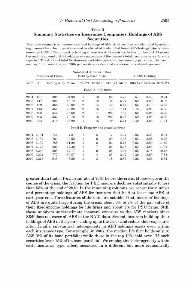
Table II reports insurers’ holdings of ABS over the period 2004 to 2010. Thefirst two columns show that the fraction of life firms holding ABS (about 85%) is
28 The required capital for business risks accounts for a relatively larger fraction of RBC forP&C firms. Therefore, although P&C firms have significantly lower leverage than life firms, theirRBC ratios are about the same.
Is Historical Cost Accounting a Panacea? 2505
Table IISummary Statistics on Insurance Companies’ Holdings of ABS
SecuritiesThis table summarizes insurers’ year-end holdings of ABS. ABS positions are identified by match-ing insurers’ bond holdings at year-end to a list of ABS identified from S&P’s Ratings IQuery usingnine-digit CUSIP. Conditional on holding at least one ABS, statistics for the number of ABS securi-ties and the amount of ABS holdings as a percentage of the insurer’s total fixed-income portfolio arereported. The ABS and total fixed-income portfolio figures are measured by par value. The mean,median, 10th percentile, and 90th percentile are calculated across insurers at each year-end.
Number of ABS SecuritiesNumber of Firms Held by Each Firm % ABS Holding
Year All Holding ABS Mean 10th Pct Median 90th Pct Mean 10th Pct Median 90th Pct
Panel A. Life firms
2004 481 391 34.99 1 10 82 4.72 0.57 3.45 9.242005 447 380 46.12 2 12 105 5.07 0.63 3.89 10.962006 429 368 60.02 2 14 146 6.45 0.65 4.79 14.232007 413 351 72.88 2 16 175 7.44 0.75 5.95 15.882008 408 342 76.69 2 17 209 7.33 0.68 6.08 15.752009 403 337 72.70 2 16 220 6.48 0.52 4.95 13.582010 384 319 68.20 1 15 198 5.41 0.40 4.26 11.61
Panel B. Property and casualty firms
2004 1,151 741 7.81 1 5 17 4.07 0.56 3.36 8.312005 1,132 764 9.52 1 6 20 4.45 0.63 3.28 8.782006 1,132 785 11.20 1 6 24 5.15 0.56 3.80 11.492007 1,173 820 12.30 1 7 26 5.48 0.63 3.83 11.572008 1,240 825 12.17 1 6 26 4.92 0.55 3.18 10.782009 1,224 777 10.87 1 4 23 3.47 0.30 2.09 7.812010 1,215 645 8.59 1 3 18 2.89 0.22 1.56 6.81
greater than that of P&C firms (about 70%) before the crisis. Moreover, over thecourse of the crisis, the fraction for P&C insurers declines substantially to lessthan 53% at the end of 2010. In the remaining columns, we report the numberand percentage holdings of ABS for insurers that hold at least one ABS ateach year-end. Three features of the data are notable. First, insurers’ holdingsof ABS are quite large during the crisis, about 6% to 7% of the par value oftheir fixed-income holdings for life firms and about 5% for P&C firms. Still,these numbers underestimate insurers’ exposure to the ABS markets sinceS&P does not cover all ABS in the NAIC data. Second, insurers build up theirholdings of ABS in the years leading up to the crisis and reduce their exposuresafter. Finally, substantial heterogeneity in ABS holdings exists even withineach insurance type. For example, in 2007, the median life firm holds only 16ABS (6% of its bond portfolio) while those in the top 10% hold over 175 suchsecurities (over 15% of its bond portfolio). We employ this heterogeneity withineach insurance type, albeit measured in a different but more economically
2506 The Journal of Finance R©
0
200
400
600
800
1,000
1,200
0
1,000
2,000
3,000
4,000
5,000
6,000
7,000
2005
Q1
2005
Q2
2005
Q3
2005
Q4
2006
Q1
2006
Q2
2006
Q3
2006
Q4
2007
Q1
2007
Q2
2007
Q3
2007
Q4
2008
Q1
2008
Q2
2008
Q3
2008
Q4
2009
Q1
2009
Q2
2009
Q3
2009
Q4
2010
Q1
2010
Q2
2010
Q3
2010
Q4
All ABS (Left scale) ABS held by insurance companies (Right scale)
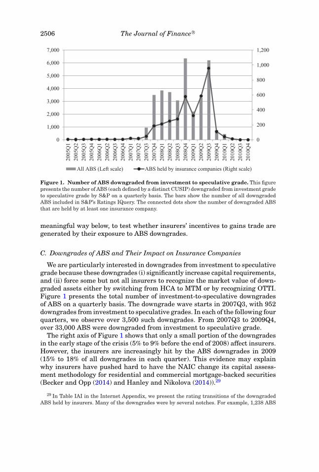
Figure 1. Number of ABS downgraded from investment to speculative grade. This figurepresents the number of ABS (each defined by a distinct CUSIP) downgraded from investment gradeto speculative grade by S&P on a quarterly basis. The bars show the number of all downgradedABS included in S&P’s Ratings IQuery. The connected dots show the number of downgraded ABSthat are held by at least one insurance company.
meaningful way below, to test whether insurers’ incentives to gains trade aregenerated by their exposure to ABS downgrades.
C. Downgrades of ABS and Their Impact on Insurance Companies
We are particularly interested in downgrades from investment to speculativegrade because these downgrades (i) significantly increase capital requirements,and (ii) force some but not all insurers to recognize the market value of down-graded assets either by switching from HCA to MTM or by recognizing OTTI.Figure 1 presents the total number of investment-to-speculative downgradesof ABS on a quarterly basis. The downgrade wave starts in 2007Q3, with 952downgrades from investment to speculative grades. In each of the following fourquarters, we observe over 3,500 such downgrades. From 2007Q3 to 2009Q4,over 33,000 ABS were downgraded from investment to speculative grade.
The right axis of Figure 1 shows that only a small portion of the downgradesin the early stage of the crisis (5% to 9% before the end of 2008) affect insurers.However, the insurers are increasingly hit by the ABS downgrades in 2009(15% to 18% of all downgrades in each quarter). This evidence may explainwhy insurers have pushed hard to have the NAIC change its capital assess-ment methodology for residential and commercial mortgage-backed securities(Becker and Opp (2014) and Hanley and Nikolova (2014)).29
29 In Table IAI in the Internet Appendix, we present the rating transitions of the downgradedABS held by insurers. Many of the downgrades were by several notches. For example, 1,238 ABS

Is Historical Cost Accounting a Panacea? 2507
What is central to our analysis is the impact of these ABS downgrades on aninsurer’s capital position, not its holdings of ABS or downgraded ABS per se.Recall that a downgrade degrades the capital position, as proxied by the RBCratio, of an insurer holding the downgraded asset in two ways: first, it increasesthe percentage capital requirement (denominator), and, second, it may force therecognition of the price decline, reducing the insurer’s statutory equity capital(numerator). Leverage amplifies these effects as they both operate throughcapital, which is only a fraction of total assets. Thus, even though life and P&Cfirms had similar portfolio allocations to ABS entering the crisis, the significantABS downgrades during the crisis impact the capital positions of life firms morethan those of P&C firms. In Table IAIII in the Internet Appendix, we reportsummary statistics on these effects, measured for each firm as the expectedchange in the RBC ratio as a result of actual ABS downgrades during the crisis(2007Q3 to 2009Q4), holding constant the insurer’s ABS positions enteringthe crisis. Hereafter we refer to this measure as “ABS exposure.” In many ofour analyses, we isolate the differential effects of accounting rules from theimpact of ABS downgrades by focusing on a subsample of 189 life and 105P&C insurers with large and similar ABS exposures. These samples represent,among insurers holding at least one downgraded ABS, the top 75% of life firmsand the top 25% of P&C firms. The cutoff exposure is approximately −0.4 onthe RBC ratio scale.
D. Accounting Treatments of Downgraded ABS by Life and P&C InsuranceCompanies
Our first identification strategy relies on the different accounting rules usedby life (HCA) and P&C (MTM) insurers for speculative-grade bonds. Exclusionrestrictions aside, we assess the relevance of this strategy by exploring thecross-sectional differences between P&C and life insurers in the use of fair, ormarket, value in booking recently downgraded ABS. Using year-end positiondata, we classify as revalued those positions for which the book and fair valuesare equal; all other positions are classified as held at HCA. Table III reportsthe revaluation frequencies for two types of downgrades: (i) from investment tospeculative grade, and (ii) from AAA to speculative grade (this case being mostsevere and unexpected).
The results in Table III show striking differences between life and P&Cinsurers, confirming the economic basis for our between-insurance-type analy-sis. For example, consider row (2), which includes all downgrades from AAA tospeculative grade over the 2005 to 2010 period. Of 1,860 ABS positions that lifeinsurers hold under HCA before the downgrades, 79% remain under HCA, 9%are revalued, and 12% are sold after the downgrades. In contrast, P&C firms
were downgraded to the BB class (for brevity, we group BB+, BB, and BB− into one class), 451of which were rated AAA before the downgrade. These dramatic shifts, which likely came as asurprise to insurers, significantly impacted the insurers’ capital positions.

2508 The Journal of Finance R©
Table IIIAccounting Treatment of Downgraded ABS
This table reports frequency statistics on insurers’ accounting treatment of downgraded ABSpreviously held at modified historical costs. Two types of downgrade are considered: (a) frominvestment to speculative grade, and (b) from AAA to speculative grade. Rows (1) and (2) includeall downgrades from 2005 to 2010, and rows (3) and (4) include only those downgrades in the fourthquarter of each year. Over the year in which the downgrade occurs, each position held at modifiedhistorical cost at the beginning of the year is reclassified into one of the following three groups: (i)kept at historical cost (HCA), (ii) kept but revalued to the year-end fair value (revalued), and (iii)sold. The percentages of these groups are reported separately for each type of downgrade and forlife and P&C insurers.
Life Firms Property & Casualty Firms
Treatment Treatmentafter Downgrade after Downgrade
Number ofPositions HCA Revalued Sold
Number ofPositions HCA Revalued Sold
Panel A. All downgrades in 2005–2010
(1) Investment tospeculative
5,161 71% 15% 14% 1,588 40% 39% 21%
(2) AAA to speculative 1,860 79% 9% 12% 851 45% 36% 20%
Panel B. Downgrades in the fourth quarter of each year
(3) Investment tospeculative
1,207 74% 14% 13% 327 20% 60% 20%
(4) AAA to speculative 514 79% 10% 11% 220 16% 63% 21%
hold 851 soon-to-be-downgraded ABS positions, of which 45% remain underHCA, 36% are revalued, and 20% are sold.
One drawback of the NAIC balance sheet data for this particular type ofanalysis is that the positions are available only at year-end. It is plausiblethat revaluations occur at different times in the year and market prices sub-sequently drift, creating a bias against finding revaluations. This may havehappened, for example, during 2009, when many of the extreme downgradestook place relatively early in the year. To address this issue, we consider asubset of downgrades that occurred in the fourth quarter, as the drift problemmay be less important for these downgrades, which are temporally closer tothe year-end measurement. As expected, the results are more striking: P&Cfirms keep only 16% of downgraded ABS under HCA, revalue 63% (six timesas much as life), and sell 21%.30
The difference in revaluation frequency between life and P&C insurers is notdue to differences in the characteristics, such as credit quality, of their ABS. InTable IAII in the Internet Appendix, we estimate several linear models for the
30 Similarly, Figure IA2 in the Internet Appendix shows that P&C firms revalue a significantlyhigher percentage of speculative-grade positions than do life firms in each year during our sampleperiod.

Is Historical Cost Accounting a Panacea? 2509
probability that an ABS position is revalued controlling for its credit quality,other distinct characteristics (e.g., issue size), and time-varying characteris-tics (e.g., maturity remaining at the end of the downgrade year). We find that,even with all these controls, P&C firms remain significantly more likely thanlife firms to revalue a downgraded position, confirming the importance of reg-ulatory accounting rules in dictating insurers’ actual accounting treatments.Taken together, this evidence supports the relevance of our first identificationstrategy and provides the economic basis for using life and P&C insurers asrepresentatives for institutions using HCA and MTM, respectively.
E. OTTI Recognition across U.S. States
Our second identification strategy relies on the fine variation in accountingpractices among the same type of insurers across domicile states. As explainedin Section I.C, we classify states as either those that strictly implement theNAIC model regulation or those that provide some level of discretion to theircommissioners. Here, we assess the economic relevance of our classificationby exploring whether the recognition of market value for accounting purposesvaries significantly across states of domicile, in line with our expectation.
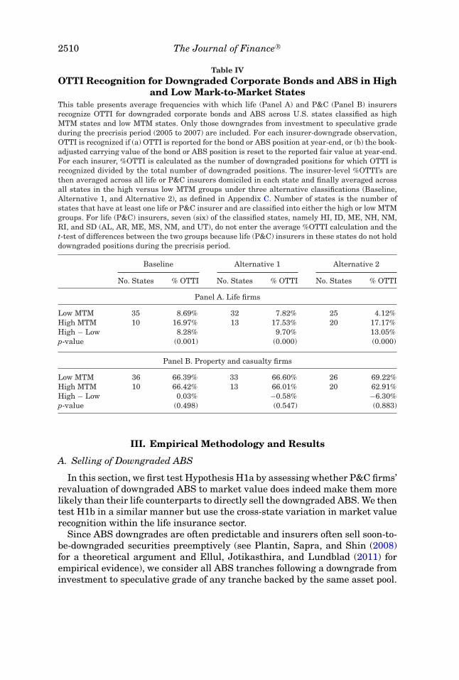
Table IV reports the average frequencies with which life (Panel A) and P&C(Panel B) insurers recognize OTTI for downgraded corporate bonds and ABS inthe precrisis period. For each insurer-downgrade observation, OTTI is consid-ered recognized if (a) OTTI is reported for the bond or ABS position at year-end,or (b) the book-adjusted carrying value of the position is reset to the reportedfair value at year-end. Thus, our definition captures both MTM and OTTI un-der HCA, reflecting the maximum degree to which each insurer recognizes thechange in market value of their downgraded holdings. For each insurer, wecalculate the OTTI frequency as the percentage of all downgraded positions forwhich OTTI is recognized. We then average the insurer-level OTTI frequenciesfor all life or P&C firms domiciled in each state and finally average across allstates in the high versus low MTM groups.
The results confirm that the precrisis level of OTTIs for life firms domiciled inhigh MTM states is larger (around 17%) than those of life firms domiciled in lowMTM states (around 4% to 9%). These differences may result from the actualexercise of regulatory discretion by the commissioners in high MTM statesand/or the concerns of life firms in these states that, if they do not properlyrecognize OTTIs, they may be penalized. In contrast, there is no difference inOTTI frequency between P&C firms in the high and low MTM states, consistentwith the notion that a departure from the NAIC guidelines only occurs incases in which the recognition of market value is discretionary. P&C insurersare required by the NAIC guidelines to use MTM. Overall, the evidence inTable IV confirms that exogenous variation in the degree of market valuerecognition does exist among life insurers domiciled in different U.S. states,thereby providing the economic basis for our within-life analysis.
2510 The Journal of Finance R©
Table IVOTTI Recognition for Downgraded Corporate Bonds and ABS in High
and Low Mark-to-Market StatesThis table presents average frequencies with which life (Panel A) and P&C (Panel B) insurersrecognize OTTI for downgraded corporate bonds and ABS across U.S. states classified as highMTM states and low MTM states. Only those downgrades from investment to speculative gradeduring the precrisis period (2005 to 2007) are included. For each insurer-downgrade observation,OTTI is recognized if (a) OTTI is reported for the bond or ABS position at year-end, or (b) the book-adjusted carrying value of the bond or ABS position is reset to the reported fair value at year-end.For each insurer, %OTTI is calculated as the number of downgraded positions for which OTTI isrecognized divided by the total number of downgraded positions. The insurer-level %OTTI’s arethen averaged across all life or P&C insurers domiciled in each state and finally averaged acrossall states in the high versus low MTM groups under three alternative classifications (Baseline,Alternative 1, and Alternative 2), as defined in Appendix C. Number of states is the number ofstates that have at least one life or P&C insurer and are classified into either the high or low MTMgroups. For life (P&C) insurers, seven (six) of the classified states, namely HI, ID, ME, NH, NM,RI, and SD (AL, AR, ME, MS, NM, and UT), do not enter the average %OTTI calculation and thet-test of differences between the two groups because life (P&C) insurers in these states do not holddowngraded positions during the precrisis period.
Baseline Alternative 1 Alternative 2
No. States % OTTI No. States % OTTI No. States % OTTI
Panel A. Life firms
Low MTM 35 8.69% 32 7.82% 25 4.12%High MTM 10 16.97% 13 17.53% 20 17.17%High − Low 8.28% 9.70% 13.05%p-value (0.001) (0.000) (0.000)
Panel B. Property and casualty firms
Low MTM 36 66.39% 33 66.60% 26 69.22%High MTM 10 66.42% 13 66.01% 20 62.91%High − Low 0.03% −0.58% −6.30%p-value (0.498) (0.547) (0.883)
III. Empirical Methodology and Results
A. Selling of Downgraded ABS
In this section, we first test Hypothesis H1a by assessing whether P&C firms’revaluation of downgraded ABS to market value does indeed make them morelikely than their life counterparts to directly sell the downgraded ABS. We thentest H1b in a similar manner but use the cross-state variation in market valuerecognition within the life insurance sector.
Since ABS downgrades are often predictable and insurers often sell soon-to-be-downgraded securities preemptively (see Plantin, Sapra, and Shin (2008)for a theoretical argument and Ellul, Jotikasthira, and Lundblad (2011) forempirical evidence), we consider all ABS tranches following a downgrade frominvestment to speculative grade of any tranche backed by the same asset pool.

Is Historical Cost Accounting a Panacea? 2511
We model the probability of selling each affected ABS by the end of the quarterin which the downgrade occurs as a linear model:
Si. j.k = κ0 + κP Pj + κV Vi, j,k + κXXi,k + κY Yj,k + κW Wk + εi, j,k, (6)
where Si. j.k is a dummy variable that equals one if insurer j sells some of itsholding in downgraded bond i by the end of event quarter k; Pj is a dummyvariable that equals one if insurer j is a P&C insurer; Vi, j,k is an dummy variablethat equals one if insurer j revalues downgraded bond i at the year-end beforeevent k; Xi,k is a vector of bond i’s static and time-varying characteristics,including the rating group dummies, immediately preceding event k; Yj,k isa vector of insurer j’s static and time-varying characteristics at the year-endprior to event k; Wk is a vector of time-specific variables for downgrade eventk; and κ ’s are the corresponding vectors of coefficients to be estimated.
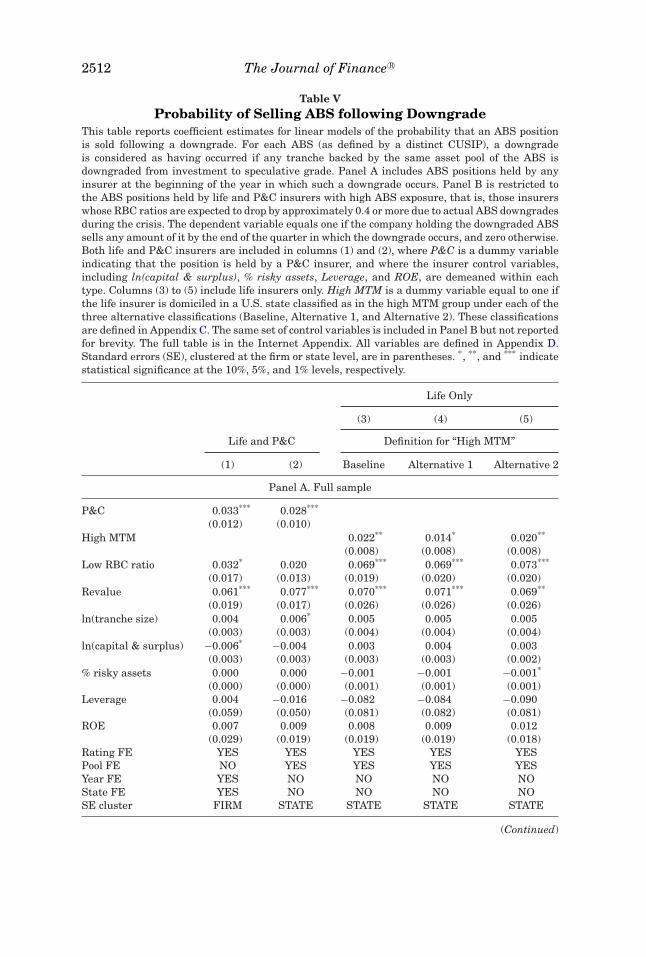
Table V reports the results. In columns (1) and (2) of Panel A, the coefficientson the P&C dummy are positive and significant. Consistent with Hypothe-sis H1a, P&C insurers, using MTM for speculative-grade ABS, have a higherpropensity to sell an ABS position affected by a downgrade than do life insur-ers, using HCA. In column (1), we include rating, state, and year dummies,thus identifying the result by comparing the selling propensities of life andP&C insurers after absorbing any variation across states, rating groups, andyear of the downgrade. In column (2), the common denominators are an ABS’srating group and asset pool. The difference in selling propensity between lifeand P&C firms is similar in both columns, at 2.8% to 3.3%, which is about halfof the unconditional selling probability of life firms.31
We include a number of control variables to capture ABS and insurer char-acteristics as well as the position’s existing accounting treatment. First, weinclude a revaluation dummy that controls for the likelihood that, regardlessof their type, insurers are more likely to sell downgraded positions that havealready been re-booked at market price, as doing so will not generate furtherlosses but will help reduce the required RBC. The significant and positive co-efficient on the revaluation dummy confirms this intuition. Second, we includeABS-level characteristics, such as liquidity. These characteristics cannot ex-plain the difference in selling propensity that we demonstrate between life andP&C firms. We also include the tranche offering amount and its initial rat-ing (before the first downgrade of the pool), which tend to be correlated withliquidity, as control variables in all columns.32
A valid concern is that our results may be driven by the fact that, due to theirlower leverage, P&C firms are generally less impacted by ABS downgrades thanare life firms. We address this concern by examining the subsample of life andP&C insurers with similar, and significant, ABS exposures. We describe theconstruction of this subsample in Section II.C. Panel B of Table V (columns (1)
31 The unconditional probability of selling downgraded ABS is 12.7% for P&C firms and 6.4%for life firms.
32 Our estimates suggest that large ABS issues are more likely to be sold, possibly due to theirsuperior liquidity.
2512 The Journal of Finance R©
Table VProbability of Selling ABS following Downgrade
This table reports coefficient estimates for linear models of the probability that an ABS positionis sold following a downgrade. For each ABS (as defined by a distinct CUSIP), a downgradeis considered as having occurred if any tranche backed by the same asset pool of the ABS isdowngraded from investment to speculative grade. Panel A includes ABS positions held by anyinsurer at the beginning of the year in which such a downgrade occurs. Panel B is restricted tothe ABS positions held by life and P&C insurers with high ABS exposure, that is, those insurerswhose RBC ratios are expected to drop by approximately 0.4 or more due to actual ABS downgradesduring the crisis. The dependent variable equals one if the company holding the downgraded ABSsells any amount of it by the end of the quarter in which the downgrade occurs, and zero otherwise.Both life and P&C insurers are included in columns (1) and (2), where P&C is a dummy variableindicating that the position is held by a P&C insurer, and where the insurer control variables,including ln(capital & surplus), % risky assets, Leverage, and ROE, are demeaned within eachtype. Columns (3) to (5) include life insurers only. High MTM is a dummy variable equal to one ifthe life insurer is domiciled in a U.S. state classified as in the high MTM group under each of thethree alternative classifications (Baseline, Alternative 1, and Alternative 2). These classificationsare defined in Appendix C. The same set of control variables is included in Panel B but not reportedfor brevity. The full table is in the Internet Appendix. All variables are defined in Appendix D.Standard errors (SE), clustered at the firm or state level, are in parentheses. *, **, and *** indicatestatistical significance at the 10%, 5%, and 1% levels, respectively.
Life Only
(3) (4) (5)
Life and P&C Definition for “High MTM”
(1) (2) Baseline Alternative 1 Alternative 2
Panel A. Full sample
P&C 0.033*** 0.028***
(0.012) (0.010)High MTM 0.022** 0.014* 0.020**
(0.008) (0.008) (0.008)Low RBC ratio 0.032* 0.020 0.069*** 0.069*** 0.073***
(0.017) (0.013) (0.019) (0.020) (0.020)Revalue 0.061*** 0.077*** 0.070*** 0.071*** 0.069**
(0.019) (0.017) (0.026) (0.026) (0.026)ln(tranche size) 0.004 0.006* 0.005 0.005 0.005
(0.003) (0.003) (0.004) (0.004) (0.004)ln(capital & surplus) −0.006* −0.004 0.003 0.004 0.003
(0.003) (0.003) (0.003) (0.003) (0.002)% risky assets 0.000 0.000 −0.001 −0.001 −0.001*
(0.000) (0.000) (0.001) (0.001) (0.001)Leverage 0.004 −0.016 −0.082 −0.084 −0.090
(0.059) (0.050) (0.081) (0.082) (0.081)ROE 0.007 0.009 0.008 0.009 0.012
(0.029) (0.019) (0.019) (0.019) (0.018)Rating FE YES YES YES YES YESPool FE NO YES YES YES YESYear FE YES NO NO NO NOState FE YES NO NO NO NOSE cluster FIRM STATE STATE STATE STATE
(Continued)
Is Historical Cost Accounting a Panacea? 2513
Table V—Continued
Life Only
(3) (4) (5)
Life and P&C Definition for “High MTM”
(1) (2) Baseline Alternative 1 Alternative 2
Panel A. Full sample
Observations 11,339 11,339 8,446 8,446 8,446R2 0.071 0.014 0.019 0.018 0.018Number of pools 2,120 2,011 2,011 2,011
Panel B. Subsample of life and P&C firms with high ABS exposure
P&C 0.040** 0.034***
(0.019) (0.010)High MTM 0.022** 0.015* 0.025***
(0.009) (0.009) (0.009)Low RBC ratio 0.060** 0.049** 0.075*** 0.075*** 0.082***
(0.028) (0.019) (0.022) (0.023) (0.023)Bond controls YES YES YES YES YESInsurer controls YES YES YES YES YESRating FE YES YES YES YES YESPool FE NO YES YES YES YESYear FE YES NO NO NO NOState FE YES NO NO NO NOSE cluster FIRM STATE STATE STATE STATEObservations 8,894 8,894 7,957 7,957 7,957R2 0.064 0.016 0.021 0.020 0.020Number of pools 2,054 1,985 1,985 1,985
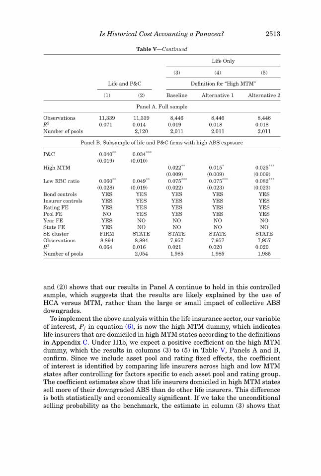
and (2)) shows that our results in Panel A continue to hold in this controlledsample, which suggests that the results are likely explained by the use ofHCA versus MTM, rather than the large or small impact of collective ABSdowngrades.
To implement the above analysis within the life insurance sector, our variableof interest, Pj in equation (6), is now the high MTM dummy, which indicateslife insurers that are domiciled in high MTM states according to the definitionsin Appendix C. Under H1b, we expect a positive coefficient on the high MTMdummy, which the results in columns (3) to (5) in Table V, Panels A and B,confirm. Since we include asset pool and rating fixed effects, the coefficientof interest is identified by comparing life insurers across high and low MTMstates after controlling for factors specific to each asset pool and rating group.The coefficient estimates show that life insurers domiciled in high MTM statessell more of their downgraded ABS than do other life insurers. This differenceis both statistically and economically significant. If we take the unconditionalselling probability as the benchmark, the estimate in column (3) shows that
2514 The Journal of Finance R©
the probability of selling downgraded ABS positions is about 34% higher thanaverage (0.022/0.064) for life insurers domiciled in high MTM states.
We next explore whether capital-constrained firms are more likely to divestdowngraded ABS, which is expected to be the case if insurers sell downgradedABS to improve their capital positions. Intuitively, insurers that start withlow RBC ratios should be pushed closer to regulatory (or other rating-related)thresholds, and thus have greater need to respond. To capture this effect, in allregressions we include a low RBC ratio dummy, which indicates insurers withRBC ratios in the lowest quartile within each type. We find that the coefficientson this dummy are positive and significant in almost all columns of Table V,Panel A (all insurers) and in all columns of Table V, Panel B (insurers withlarge ABS exposures). The economic effects, ranging from 2.0% to 8.2%, are sig-nificant given the relatively small unconditional selling probability. Moreover,as expected, these effects are stronger in the sample of insurers with large ABSexposures.
Overall, the results in Table V, obtained from both between-insurance-typeand within-life analyses, consistently demonstrate that insurers that are re-quired to use MTM (or recognize OTTI) for downgraded ABS are more likelyto sell their downgraded holdings than insurers that can continue to use HCA.This result is consistent with General Hypothesis 1, and the general predictionof the theoretical literature.
B. Gains Trading
In this section, we assess insurers’ propensity to gains trade by examiningthe extent to which an insurer’s decision to sell a bond position is motivatedby its unrealized gain. For each position, we calculate the unrealized gain asthe difference between the position’s book-adjusted carrying value and fairvalue, which is measured as a percentage of its book-adjusted carrying value.If the insurer engages in gains trades, it should be more likely to sell a bondposition with an unrealized gain than an otherwise similar position with anunrealized loss. Thus, to identify gains trading, we need assets that are both(i) held under HCA and (ii) have sufficient cross-sectional variation, wherebysome positions carry unrealized gains while others carry unrealized losses. Theformer condition essentially rules out equities. The latter condition rules outABS and structured products, as most of them carry extremely large unrealizedlosses.33 This leaves us with government and corporate bonds, which togetheraccount for over 70% of invested assets for both life and P&C insurers. Insurerscan choose any combination of these two asset classes to gains trade, dependingon the availability of unrealized gains in each.
33 In Table IAV in the Internet Appendix, we report the distribution of the percentage of unreal-ized gains (and losses) separately for life and P&C firms. Panel A corresponds to ABS, Panel B tocorporate bonds, and Panel C to government bonds. Panel A shows that over 90% of ABS positionscarry unrealized losses in 2008 (with the median as large as −30%), and over 75% still do in 2009.Panels B and C show that unrealized gains (of various magnitudes) are much more available forcorporate and government bonds.

Is Historical Cost Accounting a Panacea? 2515
B.1. Propensity to Gains Trade and ABS Exposure
We model the probability of selling a bond position as a linear model:
Si, j,q = γ0 + (γz + γzyyj,q + γzccq + γzyc yj,qcq
)zi, j,q
+ γXXi,q + γY Yj,q + γW Wq + εi, j,q, (7)
where Si, j,q is a dummy variable that equals one if insurer j sells bond i incalendar quarter q; zi, j,q is the unrealized gain percentile (ranging from zero toone) of bond i in the portfolio of insurer j at the year-end prior to quarter q; yj,qis a characteristic of insurer j that is expected to amplify or diminish the effectof zi, j,q, measured at the year-end prior to quarter q; cq is a dummy variablethat equals one if quarter q lies in the crisis period; Xi,q is a vector of static andtime-varying characteristics of bond i, including rating group dummies, at thebeginning of quarter q; Yj,q is a vector of financial and risk characteristics ofinsurer j at the year-end prior to quarter q; Wq is a vector of calendar-quarterdummies interacted with a bond-type dummy (government vs. corporate)34;and the γ ’s are the corresponding coefficients to be estimated. Depending onthe specification, we also include either domicile state fixed effects or firm fixedeffects in Yj,q.
Our coefficients of interest are the γz’s, both the main term and the interactionterms. We interpret a positive coefficient as evidence for gains trading, since itindicates that positions that carry higher unrealized gains are more likely to besold. Similarly, positive (negative) coefficients on the interaction terms indicatea larger (smaller) degree of gains trading during the crisis (cq = 1) and/or forinsurers with a certain characteristic as captured by yj,q.
We first test Hypothesis H2a. We estimate our probability model for a sampleof life and P&C insurers that are affected by ABS downgrades (i.e., the sampleof insurers in Panel A of Table V), and include in the model the interactionbetween the unrealized gain percentile and a high ABS exposure dummy. IfH2a is true, then we expect the coefficient on the interaction term to be positivefor the crisis period.
Table VI reports the results. We start by investigating the crisis period inisolation. In columns (1) and (4), the coefficients on the interaction between theunrealized gain percentile and the high ABS exposure dummy are positive andsignificant (at the 1% level for life and 10% level for P&C insurers), indicatingthat both life and P&C insurers with high ABS exposure engage in a greaterdegree of gains trading than do other insurers of the same type. These resultsare identified by comparing the degree of gains trading between firms withhigh and low ABS exposure, holding constant bond characteristics including
34 We interact calendar-quarter with bond-type dummies to identify gains trading from otheralternative forces that may drive insurers to sell mostly government or corporate bonds. This is aconcern since, during the crisis, government bonds as a group carry significantly larger unrealizedgains than corporate bonds. In robustness checks in the Internet Appendix (Tables IAVI, IAVIII,and IAXI), we separately consider corporate bonds and government bonds and show that our mainfindings hold in both samples.

2516 The Journal of Finance R©
Table VIDo Exposures to Downgraded ABS Induce Gains Trading?
This table reports coefficient estimates for linear models of the probability that an insurancecompany holding at least one downgraded ABS will sell a corporate or government bond position.The dependent variable is a dummy that equals one if the insurer holding the bond at the beginningof the quarter sells the bond during the quarter, and zero otherwise. The regressions are runseparately for life insurers (columns (1) to (3)) and P&C insurers (columns (4) to (6)). The variablesof interest are Unrealized gain pct. and its interactions with the crisis and high ABS exposuredummies. Corp (Gov) is a dummy variable equal to one for corporate bond (government bond)positions, and zero otherwise. Bond characteristics are interacted with these bond-type dummies.All variables, including fixed effects, are defined in Appendix D. Standard errors (SE), eithertwo-way clustered by insurer and calendar quarter or one-way clustered by calendar quarter,are in parentheses. *, **, and *** indicate statistical significance at the 10%, 5%, and 1% levels,respectively.
Life Property & Casualty
(1) (2) (3) (4) (5) (6)
Crisis All All Crisis All All
Main variables(1) Unrealized gain pct. −0.004 −0.023*** −0.023*** −0.003 −0.002 −0.000
(0.008) (0.007) (0.005) (0.004) (0.005) (0.004)(1) × (2) 0.021*** 0.001 0.000 0.015* −0.003 −0.009*
(0.006) (0.006) (0.003) (0.009) (0.007) (0.005)Crisis × (1) 0.022** 0.021** 0.001 −0.000
(0.010) (0.009) (0.006) (0.005)Crisis × (1) × (2) 0.020*** 0.019*** 0.017* 0.022*
(0.008) (0.005) (0.010) (0.011)Related insurer controls(2) High ABS exposure 0.000 −0.001 0.015** 0.015*
(0.005) (0.008) (0.007) (0.008)(3) Low RBC ratio 0.024*** 0.011** 0.008 0.002 0.004 0.012**
(0.007) (0.005) (0.005) (0.005) (0.005) (0.006)(4) Revalue 0.062*** 0.047*** 0.048*** 0.013* 0.014* 0.017**
(0.012) (0.010) (0.012) (0.007) (0.008) (0.007)Crisis × (2) 0.001 0.001 −0.001 −0.004
(0.007) (0.003) (0.007) (0.007)Crisis × (3) 0.009 0.007 −0.002 −0.004
(0.007) (0.005) (0.005) (0.004)Crisis × (4) 0.019 0.017 −0.009 −0.009
(0.012) (0.015) (0.014) (0.011)Bond controlsCorp × ln(bond age) −0.006*** −0.007*** −0.006*** −0.006** −0.007*** −0.005***
(0.002) (0.002) (0.001) (0.002) (0.002) (0.001)Corp × ln(maturity) −0.011*** −0.008*** −0.009*** −0.002 0.001 −0.004*
(0.002) (0.001) (0.001) (0.002) (0.002) (0.002)Corp × ln(issue size) 0.012*** 0.011*** 0.009*** 0.009*** 0.009*** 0.007***
(0.001) (0.001) (0.000) (0.001) (0.001) (0.001)Corp × Bankruptcy 0.262*** 0.274*** 0.275*** 0.179*** 0.200*** 0.200***
(0.020) (0.028) (0.028) (0.066) (0.063) (0.046)Corp × Downgrade 0.040*** 0.078*** 0.079*** 0.133*** 0.154*** 0.153***
(0.015) (0.022) (0.022) (0.030) (0.028) (0.026)
(Continued)

Is Historical Cost Accounting a Panacea? 2517
Table VI—Continued
Life Property & Casualty
(1) (2) (3) (4) (5) (6)
Crisis All All Crisis All All
Gov × ln(bond age) −0.034*** −0.033*** −0.032*** −0.032*** −0.036*** −0.035***
(0.007) (0.006) (0.004) (0.007) (0.005) (0.004)Gov × ln(maturity) −0.017*** −0.017*** −0.015*** −0.000 −0.004 −0.004**
(0.004) (0.004) (0.002) (0.004) (0.003) (0.002)Other insurer controlsln(capital & surplus) 0.001 0.001 0.009** −0.000 −0.000 0.014
(0.001) (0.001) (0.004) (0.002) (0.002) (0.012)% risky assets 0.000 0.000** 0.000 0.000* 0.000** −0.000
(0.000) (0.000) (0.000) (0.000) (0.000) (0.000)Leverage 0.026 0.017 0.063 0.016 0.003 −0.003
(0.024) (0.023) (0.042) (0.024) (0.020) (0.056)ROE 0.004 −0.002 0.005 −0.030* −0.038*** −0.023
(0.006) (0.004) (0.003) (0.017) (0.012) (0.014)Rating FE YES YES YES YES YES YESQuarter × Type FE YES YES YES YES YES YESState FE YES YES NO YES YES NOFirm FE NO NO YES NO NO YESSE cluster 1 FIRM FIRM QTR FIRM FIRM QTRSE cluster 2 QTR QTR – QTR QTR –Observations 790,559 1,854,938 1,854,938 305,876 742,777 742,777R2 (within) 0.027 0.022 0.014 0.026 0.023 0.013
credit rating, firm characteristics including domicile state, and the calendarquarter in which the trading takes place. In economic terms (and relative toan otherwise similar position held by insurers with low ABS exposure), aninterquartile increase in unrealized gain percentile increases the probabilitythat a corporate or government bond position will be sold in a quarter by 1.1%(0.021 × 0.5, or 30% from the mean of 3.7%) for life firms and 0.8% (0.015 ×0.5, or 13% from the mean of 6.1%) for P&C firms.
The coefficients on the control variables are generally intuitive. For example,in all models, the coefficients on the revalue dummy are significantly positive,suggesting that these positions may be held for trading rather than as a long-term investment. We also control for bond liquidity using bond age and issuesize, and find that the probability of being sold is higher for more liquid bonds,consistent with the notion that insurers actively try to minimize any priceimpact.35 Other significant control variables include a dummy that measureswhether the bond is downgraded to speculative grade, a dummy that captureswhether the bond issuer files for bankruptcy, and, depending on the model, theproportion of risky assets in an insurer’s portfolio (capturing the insurer’s riskappetite or capacity to bear risk) as well as the insurer’s ROE.
35 See Edwards, Harris, and Piwowar (2007), Hong and Warga (2000), and Schultz (2001).Driessen (2005) uses bond age to identify the liquidity component of credit spreads.
2518 The Journal of Finance R©
A criticism against looking at the crisis period in isolation is that certainfirms may gains trade even in normal times (Carey (1994)), in which case theresults in columns (1) and (4) of Table VI may have nothing to do with thesizeable ABS downgrades during the crisis. To address this criticism, we inves-tigate gains trading over the full sample period (2004 to 2010) and introducethe crisis dummy to compare insurers’ behavior during the crisis with theirbehavior in normal times. This specification thus has the important advantageof isolating incremental behavior during the crisis from common behavior thatmay be present in all periods. The two variables of interest are (i) the inter-action between the crisis dummy and the unrealized gain percentile, whichcaptures the incremental propensity to gains trade, and (ii) the triple inter-action between (i) and the high ABS exposure dummy, which captures theextent to which gains trading differs between insurers with high and low ABSexposure.
Column (2) of Table VI shows that life insurers are less likely to sell bondswith high unrealized gains in normal times (possibly to avoid paying taxes) butmore likely to do so during the crisis, consistent with Laux and Leuz’s (2009,2010) conjecture that financial institutions may gains trade to relieve finan-cial stress.36 More importantly, the coefficient on the triple interaction showsthat this gains trading behavior is significantly more pronounced among lifeinsurers with high ABS exposure. Column (3), which includes firm fixed effects,confirms that this result is not driven by firm-level time-invariant unobservedheterogeneity, and columns (5) and (6) show that a similar effect is also presentamong P&C firms. Together, the results in Table VI are consistent with Hypoth-esis H2a, and highlight the importance of ABS downgrades in driving gainstrading among insurance firms.
B.2. Propensity to Gains Trade and Capital Positions
We now test Hypothesis H2b, which posits that insurers gains trade to man-age their RBC ratio (as opposed to net income, for example). In this test, weuse the subsample of insurers that we identify as having high ABS exposure,rather than the entire sample of affected insurers as in Table VI. Doing soallows us to focus on the most relevant insurers and to hold relatively constantthe impact of ABS downgrades without overly complicating the model withtriple or quadruple interaction terms.
Table VII reports the results. We first examine whether we have suffi-cient power to identify gains trading among this subset of insurers with highABS exposure. Focusing on the first and fourth rows, columns (1) and (2) ofTable VII show that we have sufficient power for life firms; columns (4) to (6)show that we also have sufficient power for P&C firms, albeit to a lesser extent.In all specifications, we include the same set of controls as in Table VI. Tak-ing the model in columns (2) and (5), which includes firm fixed effects, as our
36 Our results also imply that reported income that includes realized gains and losses may notbe informative about insurers’ financial performance, consistent with the findings of Nissim (2012).
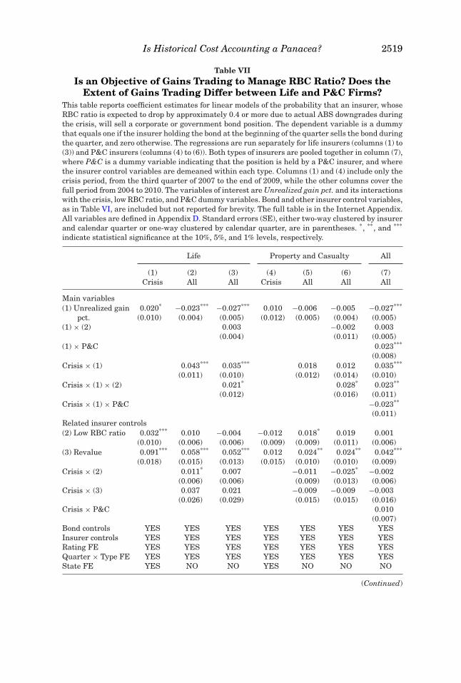
Is Historical Cost Accounting a Panacea? 2519
Table VIIIs an Objective of Gains Trading to Manage RBC Ratio? Does the
Extent of Gains Trading Differ between Life and P&C Firms?This table reports coefficient estimates for linear models of the probability that an insurer, whoseRBC ratio is expected to drop by approximately 0.4 or more due to actual ABS downgrades duringthe crisis, will sell a corporate or government bond position. The dependent variable is a dummythat equals one if the insurer holding the bond at the beginning of the quarter sells the bond duringthe quarter, and zero otherwise. The regressions are run separately for life insurers (columns (1) to(3)) and P&C insurers (columns (4) to (6)). Both types of insurers are pooled together in column (7),where P&C is a dummy variable indicating that the position is held by a P&C insurer, and wherethe insurer control variables are demeaned within each type. Columns (1) and (4) include only thecrisis period, from the third quarter of 2007 to the end of 2009, while the other columns cover thefull period from 2004 to 2010. The variables of interest are Unrealized gain pct. and its interactionswith the crisis, low RBC ratio, and P&C dummy variables. Bond and other insurer control variables,as in Table VI, are included but not reported for brevity. The full table is in the Internet Appendix.All variables are defined in Appendix D. Standard errors (SE), either two-way clustered by insurerand calendar quarter or one-way clustered by calendar quarter, are in parentheses. *, **, and ***
indicate statistical significance at the 10%, 5%, and 1% levels, respectively.
Life Property and Casualty All
(1) (2) (3) (4) (5) (6) (7)Crisis All All Crisis All All All
Main variables(1) Unrealized gain 0.020* −0.023*** −0.027*** 0.010 −0.006 −0.005 −0.027***
pct. (0.010) (0.004) (0.005) (0.012) (0.005) (0.004) (0.005)(1) × (2) 0.003 −0.002 0.003
(0.004) (0.011) (0.005)(1) × P&C 0.023***
(0.008)Crisis × (1) 0.043*** 0.035*** 0.018 0.012 0.035***
(0.011) (0.010) (0.012) (0.014) (0.010)Crisis × (1) × (2) 0.021* 0.028* 0.023**
(0.012) (0.016) (0.011)Crisis × (1) × P&C −0.023**
(0.011)Related insurer controls(2) Low RBC ratio 0.032*** 0.010 −0.004 −0.012 0.018* 0.019 0.001
(0.010) (0.006) (0.006) (0.009) (0.009) (0.011) (0.006)(3) Revalue 0.091*** 0.058*** 0.052*** 0.012 0.024** 0.024** 0.042***
(0.018) (0.015) (0.013) (0.015) (0.010) (0.010) (0.009)Crisis × (2) 0.011* 0.007 −0.011 −0.025* −0.002
(0.006) (0.006) (0.009) (0.013) (0.006)Crisis × (3) 0.037 0.021 −0.009 −0.009 −0.003
(0.026) (0.029) (0.015) (0.015) (0.016)Crisis × P&C 0.010
(0.007)Bond controls YES YES YES YES YES YES YESInsurer controls YES YES YES YES YES YES YESRating FE YES YES YES YES YES YES YESQuarter × Type FE YES YES YES YES YES YES YESState FE YES NO NO YES NO NO NO
(Continued)

2520 The Journal of Finance R©
Table VII—Continued
Life Property and Casualty All
(1) (2) (3) (4) (5) (6) (7)Crisis All All Crisis All All All
Main variablesFirm FE NO YES YES NO YES YES YESSE cluster 1 FIRM QTR QTR FIRM QTR QTR QTRSE cluster 2 QTR – – QTR – – –Observations 647,893 1,512,622 1,512,622 62,655 151,038 151,038 1,663,660R2 (within) 0.028 0.015 0.015 0.046 0.015 0.015 0.013
starting point, in columns (3) and (6) we add the interaction between the un-realized gain percentile and low RBC ratio. We also add the triple interactionwith the crisis dummy to identify the extent to which the differential propen-sity to gains trade between insurers with healthy and low RBC ratios increasesduring the crisis. If Hypothesis H2b holds, then we expect the coefficient onthis triple interaction to be positive, which turns out to be the case for both lifeand P&C firms. In normal times, insurers with a low RBC ratio do not behavedifferently from others. During the crisis, however, they engage in a higherdegree of gains trading. Take life insurers, for example. Among those with ahealthy RBC ratio (taking their behavior in normal times as a benchmark), aninterquartile increase in the unrealized gain percentile increases the probabil-ity that a corporate or government bond position will be sold in a quarter by1.8% (0.035 × 0.5) during the crisis. The same effect would be 2.8% (0.056 ×0.5), significantly higher, if the position were instead held by life firms with alow RBC ratio.
B.3. Life versus P&C Insurance Companies
We now turn to the most important tests of our paper: do financial institutionsthat use MTM for downgraded assets engage in less gains trading than othersthat use HCA? In this subsection, we use the distinction between P&C and lifeinsurers as a proxy for institutions that use MTM versus those that use HCA,respectively. In the next subsection, we instead use the variation in degreesof market value recognition across life insurers domiciled in high versus lowMTM states.
Hypothesis H2c states that on average life firms gains trade more thanP&C firms. This is because the latter have already sold a larger number ofdowngraded ABS positions, and doing so alleviates the need to employ gainstrading. The results in Table VI and the first six columns of Table VII providesuggestive evidence. First, in Table VI, the effect of an interquartile increasein the unrealized gain percentile on the probability that a bond position willbe sold during the crisis is stronger for life firms (1.1%, or 30% increase fromthe mean of 3.7%) than for P&C firms (0.8%, or 13% increase from the mean of

Is Historical Cost Accounting a Panacea? 2521
6.1%). Second, while gains trading is widespread among life firms with largeABS exposures (columns (1) to (3) of Table VII), only P&C firms with large ABSexposures plus a low RBC ratio exhibit a significant degree of gains trading(columns (4) to (6) of Table VII). This select group consists of only 28 out of the105 P&C firms with large ABS exposures (and over 1,000 P&C firms in our fullsample).
In column (7) of Table VII, we formally test the difference in gains tradingbetween life and P&C insurers controlling for all other effects, including thedirect effects of ABS exposures and RBC ratios, which we have considered sofar. We include both insurance types in the estimation but introduce a P&Cdummy to distinguish the degree of gains trading between the two types. Ourcoefficient of interest, in the sixth row, is that on the triple interaction amongthe crisis dummy, P&C dummy, and unrealized gain percentile. The estimate isnegative and significant, consistent with Hypothesis H2c. In economic terms,the effect of an interquartile increase in the unrealized gain percentile on theprobability of being sold during the crisis is about 1.2% smaller (−0.023×0.5)for a bond position held by P&C firms than an otherwise similar position held bylife firms. This is highly significant given the unconditional selling probabilitiesof 4.2% and 8.0% for life and P&C firms, respectively, with large ABS exposures.Taken together, the results in Table VI and especially in Table VII provide clearevidence that P&C firms, using MTM for downgraded ABS, engage in less gainstrading than life firms, using HCA.
B.4. Life Insurance Companies in High Versus Low MTM States
We now investigate gains trading behavior within the life insurance sector,exploiting the variation in the implementation of NAIC model regulation acrossU.S. states. Hypothesis H2d predicts that life insurers domiciled in high MTMstates have a lower propensity to engage in gains trading relative to life insur-ers domiciled in low MTM states. We test this hypothesis using the sample oflife insurers with large ABS exposures.
Table VIII reports the results. In columns (1) to (3), we look at the crisis periodin isolation. The variable of interest is the interaction between the high MTMdummy and the unrealized gain percentile (the second row), which capturesthe difference in gains trading propensity, if any, between life insurers in highand low MTM states. In columns (4) to (6), we employ the full sample period,taking normal times as a benchmark. In these specifications, the variable ofinterest is the triple interaction between the crisis dummy, high MTM dummy,and unrealized gain percentile (the fourth row).
All columns of Table VIII point to the same conclusion: while life insurersgenerally tend to gains trade during the crisis, those domiciled in high MTMstates have a lower propensity to do so as compared to life insurers domiciled inlow MTM states. These results are robust across all alternative classificationsof U.S. states as described in Appendix C. Take the estimates in column (4),for example. The positive and significant coefficient of 0.051 in the third rowshows that gains trading is prevalent in this sample of life insurers (which we

2522 The Journal of Finance R©
Table VIIIDoes the Extent of Gains Trading Differ for Life Firms
in Different U.S. States?This table reports coefficient estimates for linear models of the probability that a life insurer,domiciled in different U.S. states, sell a corporate or government bond position. The sample includeslife insurers whose RBC ratios are expected to drop by approximately 0.4 or more due to actualABS downgrades during the crisis. The dependent variable is a dummy that equals one if the lifeinsurer holding the bond at the beginning of the quarter sells the bond during the quarter, andzero otherwise. The variables of interest are Unrealized gain pct. and its interactions with thecrisis and high MTM dummies. High MTM is a dummy indicating that life insurers are domiciledin high MTM states under each alternative definition, as defined in Appendix C. Bond and otherinsurer control variables, as in Table VI, are included in all models but not reported for brevity.The full table is in the Internet Appendix. All variables are defined in Appendix D. Standard errors(SE), either two-way clustered by insurer and calendar quarter or one-way clustered by calendarquarter, are in parentheses. *, **, and *** indicate statistical significance at the 10%, 5%, and 1%levels, respectively.
Crisis All
(1) (2) (3) (4) (5) (6)
Baseline Alt. 1 Alt. 2 Baseline Alt. 1 Alt. 2
Main variables(1) Unrealized gain 0.026** 0.028** 0.022* −0.023*** −0.023*** −0.025***
pct. (0.012) (0.013) (0.012) (0.005) (0.005) (0.005)(1) × High MTM −0.017** −0.017** −0.012** −0.001 −0.000 0.004
(0.007) (0.008) (0.006) (0.004) (0.004) (0.003)Crisis × (1) 0.051*** 0.052*** 0.048***
(0.013) (0.013) (0.012)Crisis × (1) × −0.018** −0.018** −0.017***
High MTM (0.007) (0.007) (0.005)
Related insurer controls(2) Low RBC ratio 0.032*** 0.032*** 0.029*** 0.010 0.010 0.010
(0.010) (0.010) (0.011) (0.006) (0.006) (0.006)(3) Revalue 0.091*** 0.091*** 0.091*** 0.059*** 0.059*** 0.059***
(0.018) (0.018) (0.020) (0.015) (0.015) (0.014)Crisis × (2) 0.012** 0.013** 0.008
(0.006) (0.006) (0.005)Crisis × (3) 0.036 0.036 0.037
(0.026) (0.026) (0.026)Crisis × 0.016*** 0.016*** 0.010**
High MTM (0.005) (0.005) (0.005)Bond controls YES YES YES YES YES YESInsurer controls YES YES YES YES YES YESRating FE YES YES YES YES YES YESQuarter × Type FE YES YES YES YES YES YESState FE YES YES YES NO NO NOFirm FE NO NO NO YES YES YESSE cluster 1 FIRM FIRM FIRM QTR QTR QTRSE cluster 2 QTR QTR QTR – – –Observations 647,893 647,893 647,893 1,512,622 1,512,524 1,512,524R2 (within) 0.028 0.028 0.028 0.015 0.015 0.014

Is Historical Cost Accounting a Panacea? 2523
show earlier in Table VII). However, the negative and significant coefficienton the triple interaction term in the fourth row indicates that life insurersin high MTM states gains trade to a lesser degree than others. In economicterms, the effect of an interquartile increase in the unrealized gain percentileon the probability of being sold during the crisis is about 0.9% smaller (−0.018× 0.5) for a bond position held by life insurers in high MTM states than anotherwise similar position held by other life insurers. This is significant giventhat the corresponding unconditional probability is only about 4.2%. Overall,these results are consistent with Hypothesis H2d.
Taken together, the tests of Hypotheses H2c and H2d provide support forGeneral Hypothesis 2. Financial institutions holding downgraded assets underHCA have a larger incentive to gains trade than other institutions holdingdowngraded assets under MTM.
C. Robustness Checks
While our results as a whole consistently show a significant impact of regula-tory accounting rules on insurers’ trading behaviors, alternative explanationsmay drive the different individual results, particularly those obtained from thecomparison between life and P&C insurers. To address this concern, we firstexamine three alternative explanations for why life firms are less likely to selldowngraded ABS but more likely to gains trade than P&C firms: (i) differencesin asset management expertise (e.g., life firms can better manage complex andilliquid assets), (ii) differences in liability or payout structures (e.g., life firmshave longer and less uncertain liabilities), and (iii) differences in tax circum-stances (e.g., life firms suffer losses during the crisis but P&C firms do not). InTable IAXIII in the Internet Appendix, we hold each of these factors roughlyconstant in a subsample of life and P&C firms and investigate the propensitiesto sell ABS (Panel A, similar to Table V) and to gains trade (Panel B, similarto column (9) of Table VII) in this subsample.37 We find that the differences intrading behavior between life and P&C insurers remain largely the same asin our baseline analyses, suggesting that these alternative explanations do notdrive our results.38
Next, we examine whether the long-term nature of life insurers’ liabilitiespermits them to hold illiquid and risky assets such as ABS when the restof the market is selling them. In Table IAXIV in the Internet Appendix, wetest this prediction by exploring characteristics of life and P&C firms’ in-vestments in (unaffiliated) common stocks (Panel A) and government bonds
37 We thank an anonymous referee for suggesting these robustness checks. For example, we holdasset management expertise constant by investigating the subsample of life and P&C insurersthat belong to a universal group with both types under the same umbrella. See the description ofTable IAXIII in the Internet Appendix for more details.
38 We concede that using life and P&C firms with similar ABS exposures does not fully addressthe concern that life firms have higher leverage than P&C firms and hence may respond differentlyto the downgrades (even if they are equally affected). Our within-life analyses, however, are freefrom this concern.

2524 The Journal of Finance R©
(Panel B).39 Life and P&C firms use the same accounting rules for each ofthese assets, so, if differences in illiquidity and risk-bearing capacities ratherthan differences in accounting rules drive our results, we should observe dif-ferences in liquidity and risk of the stock and government bond investmentsthat show up during the crisis. We do not find evidence consistent with thisprediction.
Finally, although our within-life identification is relatively free from endo-geneity concerns, one may still argue that the discretion provided to state insur-ance commissioners is correlated with the sophistication in asset managementof state-domiciled insurers and that it is the asset management sophisticationthat drives our results. We address this concern in two ways. First, we simplynote that states that are “financial centers” show up in both the high MTMgroup (e.g., CA, DE, and NY) and the low MTM group (e.g., CT, IL, and MA), inwhich case asset management sophistication is not likely to explain differencesin trading behavior between the two groups. Second, in Table IAXVII in theInternet Appendix, we repeat our ABS selling and gains trading analyses onthe subsamples of large insurers and public insurers, which arguably are moresophisticated groups. Our results continue to hold.
IV. Price Distortions
The literature convincingly demonstrates that fire sales of downgraded as-sets can generate significant price distortions (Ellul, Jotikasthira, and Lund-blad (2011) and Merrill et al. (2013), for example). In this section, we examinethis relation for bonds that are targeted for gains trading. Our goal is to shedlight on the debate on whether HCA helps to completely avoid market distor-tions and spillover effects during a financial crisis.40
We focus on corporate bonds since government bonds are highly liquid andthus unlikely to suffer price pressure from selective selling. Our identificationrelies on the cross-section of similar corporate bonds subject to different degreesof gains trading. If a large number of insurers conduct gains trading using thesame bonds in an illiquid market, these bonds are likely to suffer significant
39 We use beta and the Amihud ratio to measure the systematic risk and illiquidity of commonstocks. We use the fraction of Treasury notes/bonds in the total government bond portfolio tomeasure the illiquidity of government bonds. We acknowledge that the choice between Treasuryand other government bonds may be driven by other considerations, such as the reaching-for-yieldhypothesis of Becker and Ivashina (2013).
40 In Figure IA3 in the Internet Appendix, we show that HCA is also associated with an over-statement of the reported RBC ratio during the crisis, as market values are substantially lowerthan book values for many assets. Huizinga and Laeven (2012) find similar results for banks. InTable IAXV, we show that the portfolio allocations to ABS evolve very differently between life andP&C insurers, as well as between life insurers domiciled in high and low MTM states. Thus, thetrading behaviors induced by different regulatory accounting rules also have portfolio and riskimplications. See Ellul et al. (2014) for a similar analysis for the precrisis period.
Is Historical Cost Accounting a Panacea? 2525
price pressure.41 To test this prediction, we estimate the following model ofquarterly bond returns:
Ri,q = β0 + (βz + βzccq
)zi,q + βXXi,q + βW Wq + εi,q, (8)
where Ri,q is the return of bond i in quarter q; zi,q is the gains-trading sellingpressure from a particular group of insurers that hold bond i at the beginningof quarter q; cq is a dummy variable that equals one if quarter q lies in thecrisis period; Xi,q is a vector of static and time-varying characteristics of bondi in quarter q; Wq is a vector of time-specific variables for quarter q; and theβ ’s are the corresponding vectors of coefficients to be estimated.
Using transaction prices from TRACE, we calculate the quarterly returnof a bond as the logged change in price from the last day of the previousquarter to the last day of the current quarter.42 If a bond trades more thanonce in a day, we use the size-weighted average trade price on the last day of aquarter.43 Our variable of interest is zi,q, which we calculate as the standardizedvalue-weighted average unrealized gain percentile across all relevant insurersholding bond i. Let Holdingi,j,q denote the par value of bond i held by insurerj at the beginning of quarter q. Then the value-weighted average unrealizedgain percentile is calculated as
[∑j (Holdingi, j,q× Unrealized Gain Pct.i, j,q)∑
j Holdingi, j,q
]×
[∑j Holdingi, j,q
Issue Sizei,q
],
where the sum is over all insurers j in the high or low MTM groups. We nextstandardize the average unrealized gain percentile by subtracting its samplemean and dividing the result by its sample standard deviation. Our objectivefor the standardization is to ensure that the sample variation is roughly thesame across the high and low MTM groups, so that the coefficients on sellingpressure from the two groups can be directly compared.
We distinguish the effect of gains trading from other effects of unrealizedgains by interacting zi,q with the crisis indicator cq, since gains-trading sellingpressure should only operate during the crisis, when insurers are hit by theABS downgrades. If gains trading creates price pressure, then βzc should be
41 Schultz (2001) estimates that insurers collectively hold about 33% to 40% of investment-gradecorporate bonds.
42 This return measure is far from perfect. First, corporate bonds do not trade every day, so thelast day on which we observe trades for each bond is often a few days before quarter-end. For thebonds in our data that do pass our screen, however, approximately 90% of the last trading daysfall in the last month of the quarter. Second, the holding period over which we measure the bondreturn may be greater than one quarter. This problem affects less than 5% of the observations. Weaddress these two problems, which result in irregular holding periods, by measuring the values of(some) control variables over the same period in which the bond return is measured.
43 Trade prices tend to be more accurate for larger trades. See Bao, Pan, and Wang (2011),Feldhutter (2012), and Jotikasthira (2008) for evidence that prices vary significantly across trans-actions, even on the same day.

2526 The Journal of Finance R©
negative.44 We include standard controls for fundamental movements in thebond price, in particular, maturity-matched Treasury and rating- and maturity-matched credit spread returns, and other bond characteristics, such as issuesize. We use the interpolated constant-maturity Treasury bond from the Fedto calculate the Treasury return. The spread return is given as the corporatebond index return minus the Treasury return, where we use the rating- andmaturity-matched Bank of America–Merrill Lynch bond index as our primarysource. We estimate model (8) by OLS, and cluster standard errors by bondissuer-calendar quarter.
Table IX reports the results. In columns (1) to (3), we conduct between-insurance-type analysis. For each bond, we calculate the standardized averageunrealized gain percentile separately for life insurers’ positions and P&C in-surers’ positions. We consider life (P&C) insurers as low (high) MTM insurers.The first two columns present clear evidence that the corporate bonds dispro-portionately targeted for gains trading statistically and economically under-perform otherwise similar bonds during the crisis. These effects are absent innormal times, consistent with the notion that gains trading is used to raisestatutory equity capital during times of stress. A one-standard-deviation in-crease in low MTM insurers’ or life firms’ average unrealized gain percentiledecreases quarterly return of bonds by 0.63%, which is highly significant giventhat the interquartile range of the abnormal return is about 4.56% during the2007 to 2009 crisis. The corresponding effect is 0.19% for high MTM insur-ers’ or P&C firms’ average unrealized gain percentile. In column (3), we findthat the pressure from life firms is significantly stronger than that from P&Cfirms—indeed, the latter largely disappears when both are included. This re-sult is consistent with our finding that gains trading is widespread among lifebut limited among P&C insurers.45
In columns (4) to (6), we conduct within-life analysis and obtain similarresults. Here, we calculate the standardized average unrealized gain percentileseparately across positions of life firms domiciled in high MTM states and thosedomiciled in low MTM states. Columns (4) and (5) show that, for both groups,their gains trading generates a significant price impact during the crisis. Incolumn (6), we find that the pressure from life firms domiciled in high MTMstates trumps, again suggesting that the lower the degree of market valuerecognition for downgraded ABS, the more widespread is gains trading and thelarger its price impact. To put these results in perspective: the price pressure isgenerated by gains trading, which originates, in part, from insurers’ exposures
44 This is because the bond return and selling pressure are contemporaneous. We find someevidence that the underperformance persists for five to six quarters, since the ABS downgradesspread through the crisis and the pressure often remains for the same bonds. The underperformingbonds eventually outperform once the pressure subsides, creating a V-shape price pattern similarto that of downgraded corporate bonds demonstrated by Ellul, Jotikasthira, and Lundblad (2011).
45 On average, life (P&C) insurers buy about 4% (3%) of the same bonds back within threemonths after selling. This number increases to about 30% (20%) if we consider substitute bondswith the same credit rating (e.g., A) and with a maturity within ±1 year of the bond sold. Thisappears rather like a wash sale, but for the sole purpose of realizing an accounting gain.

Is Historical Cost Accounting a Panacea? 2527
Table IXImpact of Gains Trading on Corporate Bond Returns
This table reports OLS coefficient estimates for regressions of quarterly corporate bond returnson gains-trading selling pressure from insurers in either the low MTM group or the high MTMgroup. For each bond i in quarter q, unstandardized low (high) MTM unrealized gain percentile
is calculated as [∑
j (Holdingi, j,q× Unrealized gain pct.i, j,q )∑j Holdingi, j,q
] × [∑
j Holdingi, j,qIssue sizei,q
], where the sum is over all
insurer j’s with high ABS exposure and in the low (high) MTM group. Low (high) MTM unrealizedgain pct. is then obtained by subtracting the unstandardized low (high) MTM unrealized gainpercentile by its sample mean and dividing the result by its sample standard deviation. In columns(1) to (3), life (P&C) insurers are low (high) MTM insurers. In columns (4) to (6), life insurersdomiciled in high (low) MTM states according to the baseline definition in Appendix C are high(low) MTM insurers. To be included, a bond must be held by at least one low MTM and onehigh MTM insurer at the beginning of the quarter. Corporate bond returns are winsorized at the2.5% and 97.5% levels. Treasury return is the logged return of the maturity-matched Treasurybond, proxied by the interpolated constant maturity Treasury bond from the Fed. Spread return isthe logged return of the maturity- and rating-matched corporate bond index minus the Treasuryreturn. The corporate bond index return is calculated using the Bank of America–Merrill Lynchbond index, adjusted for the duration difference between the index and each individual bond.Bond controls, including ln(bond age), ln(issue size), ln(maturity), and downgrade and bankruptcydummies, are included in all models but not reported for brevity. The full table is in the InternetAppendix. All other variables are defined in Appendix D. Standard errors, two-way clustered bybond issuer and calendar quarter, are in parentheses. *, **, and *** indicate statistical significanceat the 10%, 5%, and 1% levels, respectively.
All: Life (Low MTM) Life Only: Low MTM Statesvs. P&C (High MTM) vs. High MTM States
(1) (2) (3) (4) (5) (6)
(1) Low MTM 0.131 0.131 0.090 0.099unrealized gain pct. (0.130) (0.126) (0.108) (0.084)Crisis × (1) −0.634** −0.620*** −0.544*** −0.414***
(0.247) (0.239) (0.202) (0.160)(2) High MTM 0.033 −0.007 0.080 −0.012unrealized gain pct. (0.053) (0.037) (0.106) (0.067)Crisis × (2) −0.193* −0.065 −0.506*** −0.142
(0.104) (0.066) (0.191) (0.089)Treasury return 0.717*** 0.725*** 0.717*** 0.648*** 0.648*** 0.648***
(0.048) (0.047) (0.048) (0.057) (0.057) (0.057)Spread return 0.691*** 0.699*** 0.692*** 0.611*** 0.612*** 0.611***
(0.061) (0.059) (0.061) (0.059) (0.059) (0.059)Bond controls YES YES YES YES YES YESRating FE YES YES YES YES YES YESQuarter FE YES YES YES YES YES YESWald test: (1) = (2) 1.73 1.19Wald test: Crisis × (1) = Crisis × (2) 7.23*** 3.08*
Observations 51,345 51,345 51,345 86,153 86,153 86,153R2 0.410 0.408 0.410 0.380 0.380 0.380
to downgraded ABS held under HCA. Our evidence therefore demonstratesspillover effects from downgraded ABS to otherwise unrelated corporate bondsthrough the interaction between HCA and regulatory capital requirements.
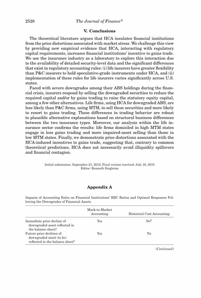
2528 The Journal of Finance R©
V. Conclusions
The theoretical literature argues that HCA insulates financial institutionsfrom the price distortions associated with market stress. We challenge this viewby providing new empirical evidence that HCA, interacting with regulatorycapital requirements, increases financial institutions’ incentive to gains trade.We use the insurance industry as a laboratory to explore this interaction dueto the availability of detailed security-level data and the significant differencesthat exist in regulatory accounting rules: (i) life insurers have greater flexibilitythan P&C insurers to hold speculative-grade instruments under HCA, and (ii)implementation of these rules for life insurers varies significantly across U.S.states.
Faced with severe downgrades among their ABS holdings during the finan-cial crisis, insurers respond by selling the downgraded securities to reduce therequired capital and/or by gains trading to raise the statutory equity capital,among a few other alternatives. Life firms, using HCA for downgraded ABS, areless likely than P&C firms, using MTM, to sell these securities and more likelyto resort to gains trading. These differences in trading behavior are robustto plausible alternative explanations based on structural business differencesbetween the two insurance types. Moreover, our analysis within the life in-surance sector confirms the results: life firms domiciled in high MTM statesengage in less gains trading and more impaired-asset selling than those inlow MTM states. Finally, we demonstrate price distortions associated with theHCA-induced incentives to gains trade, suggesting that, contrary to commontheoretical predictions, HCA does not necessarily avoid illiquidity spilloversand financial contagion.
Initial submission: September 21, 2012; Final version received: July 16, 2015Editor: Kenneth Singleton
Appendix A
Impacts of Accounting Rules on Financial Institutions’ RBC Ratios and Optimal Responses Fol-lowing the Downgrades of Financial Assets
Mark-to-MarketAccounting Historical Cost Accounting
Immediate price decline ofdowngraded asset reflected inthe balance sheet?
Yes Nob
Future price declines ofdowngraded asset (to be)reflected in the balance sheet?
Yes No
(Continued)
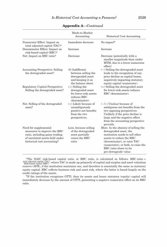
Is Historical Cost Accounting a Panacea? 2529
Appendix A—Continued
Mark-to-MarketAccounting Historical Cost Accounting
Numerator Effect: Impact ontotal adjusted capital (TAC)a
Immediate decrease No impactb
Denominator Effect: Impact onrisk-based capital (RBC)a
Increase Increase
Net: Impact on RBC ratioa Decrease Decrease (potentially with asmaller magnitude than underMTM, due to a lower numeratoreffect)
Accounting Perspective: Sellingthe downgraded asset?
(0) Indifferentbetween selling thedowngraded assetand keeping it onthe balance sheet.
(−) Selling the downgraded assetleads to the recognition of anyprice decline as capital losses,negatively impacting statutoryequity capital (numerator).
Regulatory Capital Perspective:Selling the downgraded asset?
(+) Selling thedowngraded assetfor lower-risk assetsreduces RBC(denominator).
(+) Selling the downgraded assetfor lower-risk assets reducesRBC (denominator).
Net: Selling of the downgradedasset?
(+) Likely because ofunambiguouslypositive net benefitsfrom the twoperspectives.
(−/+) Unclear because ofambiguous net benefits from thetwo opposing perspectives.Unlikely if the price decline islarge and the negative effectfrom the accounting perspectiveprevails.
Need for supplementalmeasures to improve the RBCratio, including gains tradingof unrelated assets held underhistorical cost accounting?
Less, because sellingof the downgradedasset partiallyraises the RBCratio.
More. In the absence of selling thedowngraded asset, theinstitution needs to sell otherassets to reduce the RBC(denominator), or raise TAC(numerator), or both, to raise theRBC ratio closer to itspre-downgrade value.
aThe NAIC risk-based capital ratio, or RBC ratio, is calculated as follows: RBC ratio =total adjusted capital (TAC)
Risk-based capital (RBC) ,where TAC is made up primarily of capital and surplus and asset valuationreserve (AVR), if the institution maintains one, and therefore is essentially the same as statutoryequity capital. RBC reflects business risk and asset risk, where the latter is based largely on thecredit ratings of the assets.
bIf the institution recognizes OTTI, then its assets and hence statutory (equity) capital willimmediately decrease by the amount of OTTI, generating a negative numerator effect on its RBCratio.

2530 The Journal of Finance R©
Appendix BNumerical Examples
We use the positions of Mid Century Insurance (company code = 21687) at the end of 2007 asthe pre-downgrade positions in Case 1, and the positions of Metropolitan Tower Life Insurance(company code = 97136) at the end of 2007 as the pre-downgrade positions in Cases 2 and3. We assume that the original ABS positions are in NAIC Class 1 and that half of thesepositions are later downgraded to Class 4. We also assume that if the insurer sells the downgradedABS, it replaces them with Class 1 bonds. The RBC ratio in each scenario is calculated according to:
RBC ratio = Total adjusted capital (TAC)Risk-based capital (RBC) = TAC∗+ABS
RBC∗+(λ×ABS) ,
where TAC∗ is the total adjusted capital, excluding the book value of ABS; ABS is the book valueof ABS; RBC∗ is the risk-based capital, excluding the portion required for holding ABS; and λ
is the percentage required capital for holding ABS (or new assets that replace the downgradedABS). For simplicity, the above formula and the following numerical examples ignore the sizefactor and covariance discount in the calculation of RBC and thus the results here are only anapproximation. Please refer to the Internet Appendix for more precise and detailed calculations,as well as the full list of assumptions.
Post-DowngradePre-Downgrade Not Sell Sell
Case 1: P&C Insurer, MTM(1) ABS 446.44 290.19 290.19(1.1) Expected impact from further price declinea 0.00 −50.09 0.00(2) TAC∗ 277.91 277.91 277.91(3) TAC = (1) + (1.1) + (2) 724.36 518.01 568.1(4) λ × ABS 1.82 17.71 1.18(4.1) Expected impact from further price decline 0.00 −3.06 0.00(5) RBC∗ 194.65 194.65 194.65(6) RBC = (4) + (4.1) + (5) 196.47 209.3 195.83RBC ratio = (3)/(6) 3.69 2.47 2.90Case 2: Life Insurer, HCA(1) ABS 766.88 766.88 498.47(2) TAC∗ 430.15 430.15 430.15(3) TAC = (1) + (2) 1,197.03 1,197.03 928.63(4) λ × ABS 3.07 76.69 1.99(5) RBC∗ 281.15 281.15 281.15(6) RBC = (4) + (5) 284.22 357.84 283.15
RBC ratio = (3)/(6) 4.21 3.35 3.28Case 3: Life Insurer, HCA with OTTI(1) ABS 766.88 498.47 498.47(2) T AC∗ 430.15 430.15 430.15(3) TAC = (1) + (2) 1,197.03 928.63 928.63(4) λ × ABS 3.07 49.85 1.99(5) RBC∗ 281.15 281.15 281.15(6) RBC = (4) + (5) 284.22 331 283.15RBC ratio = (3)/(6) 4.21 2.81 3.28
aThe precise rule for MTM is “the lower of book or market value.” The insurer can only lose from aprice decline but not gain from a price increase. We therefore value the expected impact of a pricedecline as a short position in a one-year at-the-money put option on B-rated ABS.

Is Historical Cost Accounting a Panacea? 2531
Appendix CClassifications of U.S. States into High and Low Mark-to-Market
GroupsThe following table lists the value of the high MTM dummy for different U.S. states, and relevantcriteria and statistics, under three classification schemes.
� The Baseline and Alternative 1 classifications are based on the insurance codes for each state.We begin by searching the insurance code to see whether the state meets Criterion A andassign the value of one if it does and zero otherwise. Criterion A: the state’s code explicitlystates or uses clear language to suggest that the Insurance Commissioner (or InsuranceDivision) has full discretion in determining the method of calculating (fixed income) assetvalues. If the state meets Criterion A, we then search the code to see whether the state alsomeets Criterion B and assign the value of one if it does and zero otherwise. (If the state doesnot meet Criterion A, we assign a value of “N/A” to Criterion B.) Criterion B: the state’s codedoes not explicitly state that the rules used by the Insurance Commissioner (or InsuranceDivision) shall not be inconsistent with the method approved by the NAIC (as set forth inthe latest edition of its publication “Valuation of Securities”). To be classified as a high MTMstate (dummy = 1) under the Baseline classification, the state has to meet both criteria. TheAlternative 1 classification expands the Baseline classification to include three additionalstates whose insurance codes, based on our reading, are ambiguous on Criterion B.
� The Alternative 2 classification is based on realized average frequencies with which life insur-ers in the state recognize OTTI for downgraded corporate bonds and ABS. Only downgradesfrom investment to speculative grade during the precrisis period (2005 to 2007) are included.For each insurer-downgrade observation, OTTI is recognized if (a) OTTI is reported for thebond or ABS position at year-end, or (b) the book-adjusted carrying value of the position isreset to the reported fair value at year-end. For each insurer, %OTTI is calculated as thenumber of downgraded positions for which OTTI is recognized divided by the total number ofdowngraded positions. The insurer-level %OTTIs are then averaged across all life insurersdomiciled in the state. States with the average %OTTI above the median are considered highMTM states (dummy = 1). Seven states in the following table, namely, HI, ID, ME, NH, NM,RI, and SD, do not have valid average %OTTI because life insurers in these states do nothold downgraded positions during the precrisis period. We do not treat these seven states ashigh MTM states in our analyses.
Classification Based on Classification Based onReading of State Insurance Code Pre-Crisis OTTI Frequency
State Baseline Alternative 1 Criterion A Criterion B Alternative 2 % OTTI
AL 0 0 1 0 1 12.44%AR 0 0 0 N/A 1 14.74%CO 0 0 0 N/A 1 21.51%CT 0 0 0 N/A 0 4.62%DC 0 0 0 N/A 1 15.38%FL 0 0 1 0 0 5.56%HI 0 0 1 0 0 –IA 0 0 1 0 0 10.47%IL 0 0 0 N/A 0 7.43%KS 0 0 0 N/A 0 5.71%KY 0 0 1 0 0 0.00%LA 0 0 0 N/A 1 27.73%MA 0 0 0 N/A 1 19.29%
(Continued)

2532 The Journal of Finance R©
Appendix C—Continued
Classification Based on Classification Based onReading of State Insurance Code Pre-Crisis OTTI Frequency
State Baseline Alternative 1 Criterion A Criterion B Alternative 2 % OTTI
MD 0 0 0 N/A 0 0.60%ME 0 0 0 N/A 0 –MN 0 0 0 N/A 0 9.63%MO 0 0 0 N/A 0 3.92%MS 0 0 0 N/A 0 0.00%NC 0 0 0 N/A 0 4.17%ND 0 0 0 N/A 0 0.00%NE 0 0 1 0 0 9.77%NH 0 0 0 N/A 0 –NJ 0 0 0 N/A 1 10.94%NM 0 0 0 N/A 0 –OK 0 0 1 0 0 3.33%OR 0 0 1 0 0 1.47%PA 0 0 0 N/A 0 5.81%RI 0 0 1 N/A 0 –SD 0 0 1 0 0 –TN 0 0 1 0 0 3.47%UT 0 0 0 N/A 1 10.99%VA 0 0 0 N/A 0 2.23%VT 0 0 1 0 0 0.00%ID 0 1 1 0/?a 0 –WA 0 1 1 0/?b 1 16.25%OH 0 1 1 0/?c 1 24.41%AZ 1 1 1 1 1 19.37%CA 1 1 1 1 1 25.00%DE 1 1 1 1 1 21.68%GA 1 1 1 1 1 14.29%IN 1 1 1 1 1 11.23%MI 1 1 1 1 1 23.05%NY 1 1 1 1 1 11.41%SC 1 1 1 1 1 20.00%TX 1 1 1 1 1 12.22%WI 1 1 1 1 1 11.42%
a“The director may adopt rules establishing standards and limitations for investments by insur-ers that are not otherwise specifically permitted or prohibited in this chapter. In the absence of arule prohibiting such, all assets shall be valued according to rules promulgated by the NationalAssociation of Insurance Commissioners (NAIC), NAIC’s valuation of securities office or by NAIC’sfinancial condition subcommittee.”
b“All bonds or other evidences of debt having a fixed term and rate held by any insurer may, ifamply secured and not in default as to principal or interest, be valued as follows . . . [description ofHCA] . . . or in lieu of such method, according to such accepted method of valuation as is approvedby the commissioner. . . . [Further conditions] The commissioner shall have full discretion indetermining the method of calculating values according to the rules set forth in this section, andnot inconsistent with any such methods then currently formulated or approved by the NationalAssociation of Insurance Commissioners.”
c“The Insurance Commissioner shall adopt rules in accordance with the Code to establish stan-dards for the determination and calculation of values, for purposes of use in statutory financialstatements submitted to the department of insurance, for those investments for which the NationalAssociation of Insurance Commissioners has not published valuation standards.”
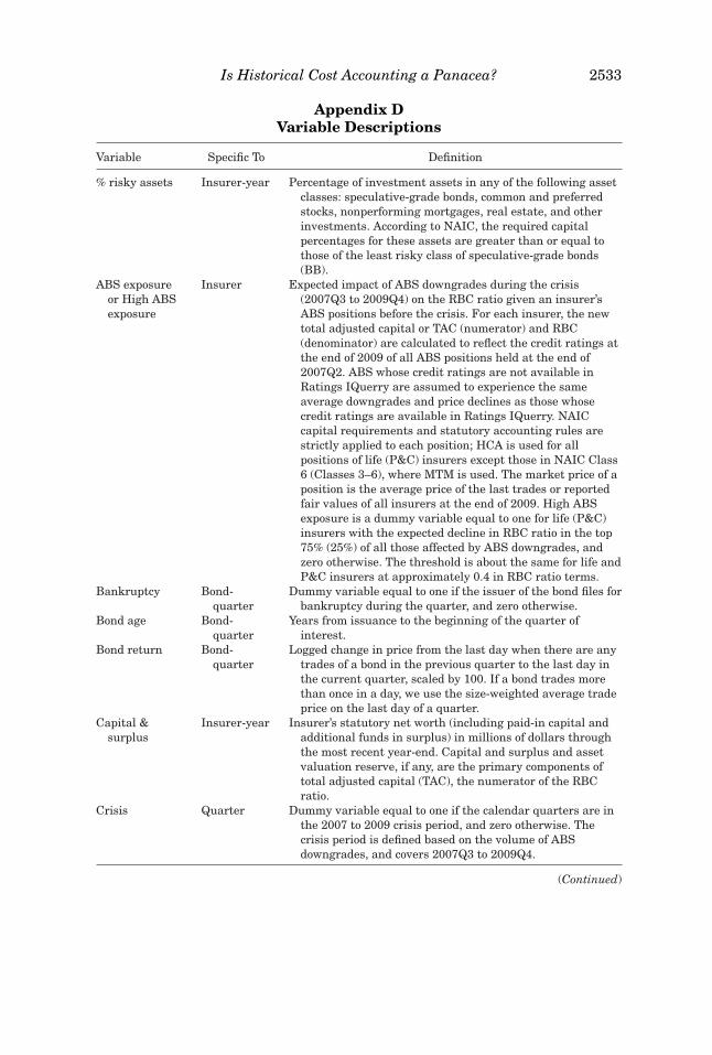
Is Historical Cost Accounting a Panacea? 2533
Appendix DVariable Descriptions
Variable Specific To Definition
% risky assets Insurer-year Percentage of investment assets in any of the following assetclasses: speculative-grade bonds, common and preferredstocks, nonperforming mortgages, real estate, and otherinvestments. According to NAIC, the required capitalpercentages for these assets are greater than or equal tothose of the least risky class of speculative-grade bonds(BB).
ABS exposureor High ABSexposure
Insurer Expected impact of ABS downgrades during the crisis(2007Q3 to 2009Q4) on the RBC ratio given an insurer’sABS positions before the crisis. For each insurer, the newtotal adjusted capital or TAC (numerator) and RBC(denominator) are calculated to reflect the credit ratings atthe end of 2009 of all ABS positions held at the end of2007Q2. ABS whose credit ratings are not available inRatings IQuerry are assumed to experience the sameaverage downgrades and price declines as those whosecredit ratings are available in Ratings IQuerry. NAICcapital requirements and statutory accounting rules arestrictly applied to each position; HCA is used for allpositions of life (P&C) insurers except those in NAIC Class6 (Classes 3–6), where MTM is used. The market price of aposition is the average price of the last trades or reportedfair values of all insurers at the end of 2009. High ABSexposure is a dummy variable equal to one for life (P&C)insurers with the expected decline in RBC ratio in the top75% (25%) of all those affected by ABS downgrades, andzero otherwise. The threshold is about the same for life andP&C insurers at approximately 0.4 in RBC ratio terms.
Bankruptcy Bond-quarter
Dummy variable equal to one if the issuer of the bond files forbankruptcy during the quarter, and zero otherwise.
Bond age Bond-quarter
Years from issuance to the beginning of the quarter ofinterest.
Bond return Bond-quarter
Logged change in price from the last day when there are anytrades of a bond in the previous quarter to the last day inthe current quarter, scaled by 100. If a bond trades morethan once in a day, we use the size-weighted average tradeprice on the last day of a quarter.
Capital &surplus
Insurer-year Insurer’s statutory net worth (including paid-in capital andadditional funds in surplus) in millions of dollars throughthe most recent year-end. Capital and surplus and assetvaluation reserve, if any, are the primary components oftotal adjusted capital (TAC), the numerator of the RBCratio.
Crisis Quarter Dummy variable equal to one if the calendar quarters are inthe 2007 to 2009 crisis period, and zero otherwise. Thecrisis period is defined based on the volume of ABSdowngrades, and covers 2007Q3 to 2009Q4.
(Continued)
2534 The Journal of Finance R©
Appendix D—Continued
Variable Specific To Definition
Downgrade Bond-quarter
Dummy variable equal to one if the bond is downgraded frominvestment to speculative grades during the quarter, andzero otherwise. S&P ratings are used wherever available.Moody’s ratings are used when S&P ratings areunavailable.
Firm FE Insurer Set of dummy variables for insurance companies to which theobservations belong.
High mark-to-market(MTM)
Insurer Dummy variable equal to one if the life insurer is domiciledin a U.S. state in the high MTM group under each of thethree alternative classifications in Appendix C, and zerootherwise.
High MTM andlow MTMunrealizedgainpercentile
Bond-quarter
Value-weighted average unrealized gain percentile across allqualified insurers’ positions in the bond, scaled by thefraction of bond issue size held by qualified insurers andthen standardized by subtracting the sample mean anddividing by the sample standard deviation. For high (low)MTM unrealized gain percentile, qualified insurers musthave positions in the bond at the beginning of the quarter,have high ABS exposure, that is, their RBC ratios areexpected to drop by approximately 0.4 or more due to actualABS downgrades during the crisis, and belong to the high(low) MTM group. In the between-insurance-type analysis,high (low) MTM insurers refer to P&C (life) insurers. In thewithin-life analysis, high (low) MTM insurers refer to lifeinsurers domiciled in high (low) MTM states.
Issue size Bond Offering amount of the bond, measured in million dollars.Leverage Insurer-year Debt as a percentage of total assets, all measured at book
values.Low RBC ratio Insurer-year Dummy variable equal to one if the insurer’s year-end RBC
ratio is in the bottom quartile among all insurers of thesame type, and zero otherwise.
Maturity Bond-quarter
Maturity of the bond at the beginning of quarter of interest,measured in years.
NAICrisk-basedcapital ratio(RBC ratio)
Insurer-year Ratio of total adjusted capital (TAC), made up primarily ofcapital and surplus and applicable valuation reserves, toNAIC risk-based capital (RBC). RBC is the minimumamount of capital that the insurance company mustmaintain based on the inherent risks in its operations. RBCis calculated based on the NAIC’s formula, which reflectsits assessment of risks of different asset classes andbusinesses. For example, a company with a RBC ratio of1.0 has capital equal to its RBC. Insurance companies withhigher RBC ratios are considered better capitalized.Insurance companies with a RBC ratio below two aresubject to supervisory intervention. The level ofsupervisory action depends on the level of the RBC ratio.Low RBC ratio dummy equals one for RBC ratios below theannual median, and zero otherwise.
(Continued)

Is Historical Cost Accounting a Panacea? 2535
Appendix D—Continued
Variable Specific To Definition
P&C Insurer Dummy variable equal to one if the insurer is a P&C firm,and zero otherwise.
Pool FE Bond Set of dummy variables for ABS tranches issued on the sameasset pool.
Quarter,Quarter ×Type, andYear FE
Quarter,Quarter-Bond type,or Year
Set of dummy variables for calendar quarters in which theobservations fall. Set of dummy variables for calendarquarters in which the observations fall, by bond type(corporate or government bonds). Set of dummy variablesfor years in which the observations fall.
Rating FE Bond-quarter
Set of dummy variables for credit rating groups, defined bythe NAIC’s RBC requirement. The groups are, in order ofcredit quality, A and above, BBB, BB, and B and below.S&P ratings are used wherever available; otherwise,Moody’s ratings are used.
Revalue Position-year
Dummy variable equal to one if the position’s book value isequal to its reported fair or market value, and zerootherwise.
ROE Insurer-year Return on equity, measured as net income divided by bookvalue of equity at the beginning of the year.
State FE Insurer-year Set of dummy variables for insurers’ domicile states.Tranche size ABS Offering amount of the ABS tranche, measured in thousand
dollars.Unrealized gain
pct.Position-
yearPercentile rank, ranging from zero to one, of the position’s
dollar unrealized gain within the insurer’s portfolio at theprevious year-end. A position’s dollar unrealized gain is thedifference between the insurer’s reported fair value andbook-adjusted carrying value of the position at the previousyear-end, measured as a percentage of book value.
REFERENCES
Allen, Franklin, and Elena Carletti, 2008, Mark-to-market accounting and cash-in-the-marketpricing, Journal of Accounting and Economics 45, 358–378.
Anand, Amber, Paul J. Irvine, Andy Puckett, and Kumar Venkataraman, 2013, Institutional trad-ing and stock resiliency: Evidence from the 2007–2009 financial crisis, Journal of FinancialEconomics 108, 773–797.
Bao, Jack, Jun Pan, and Jiang Wang, 2011, The illiquidity of corporate bonds, Journal of Finance66, 911–946.
Beatty, Anne, Sandra L. Chamberlain, and Joseph Magliolo, 1995, Managing financial reportsof commercial banks: The influence of taxes, regulatory capital and earnings, Journal ofAccounting Research 33, 231–261.
Becker, Bo, and Victoria Ivashina, 2013, Reaching for yield in the bond market, Journal of Finance70, 1863–1902.
Becker, Bo, and Marcus Opp, 2014, Regulatory reform and risk taking, Working paper, StockholmSchool of Economics.
Berger, Allen N., Richard J. Herring, and Giorgio P. Szego, 1995, The role of capital in financialinstitutions, Journal of Banking and Finance 19, 393–430.
Berry-Stolzle, Thomas R., Gregory P. Nini, and Sabine Wende, 2014, External financing in thelife insurance industry: Evidence from the financial crisis, Journal of Risk and Insurance 81,529–562.
2536 The Journal of Finance R©
Bleck, Alexander, and Xuewen Liu, 2007, Market transparency and the accounting regimes, Jour-nal of Accounting Research 45, 229–256.
Boyson, Nicole, Jean Helwege, and Jan Jindra, 2011, Crises, liquidity shocks, and fire sales atfinancial institutions, Working paper, University of South Carolina.
Carey, Mark, 1994, Snacking and smoothing: Gains trading of investment account securities bycommercial banks, Working paper, Board of Governors of the Federal Reserve System.
Driessen, Joost, 2005, Is default event risk priced in corporate bonds? Review of Financial Studies18, 165–195.
Duffie, Darrell, 2010, Presidential address: Asset price dynamics with slow-moving capital, Journalof Finance 65, 1237–1267.
Eccher, Eccher A., K. Ramesh, and S. Ramu Thiagarajan, 1996, Fair value disclosures by bankholding companies, Journal of Accounting and Economics 22, 79–117.
Edwards, Amy, Lawrence Harris, and Michael Piwowar, 2007, Corporate bond market transactioncosts and transparency, Journal of Finance 62, 1421–1451.
Ellul, Andrew, Chotibhak Jotikasthira, and Christian T. Lundblad, 2011, Regulatory pressure andfire sales in the corporate bond market, Journal of Financial Economics 101, 596–620.
Ellul, Andrew, Chotibhak Jotikasthira, Christian T. Lundblad, and Yihui Wang, 2014, Mark-to-market accounting and systemic risk: Evidence from the insurance industry, Economic Policy29, 297–341.
Feldhutter, Peter, 2012, The same bond at different prices: Identifying search frictions and sellingpressures, Review of Financial Studies 25, 1155–1206.
Goh, Beng W., Dan Li, Jeffrey Ng, and Kevin O. Yong, 2015, Market pricing of banks’ fair valueassets reported under SFAS 157 during the 2008 economic crisis, Journal of Accounting andPublic Policy 34, 129–145.
Hanley, K. Weiss, and Stanislava Nikolova, 2014, The removal of credit ratings from capitalregulation: Implications for systemic risk, Working paper, University of Maryland.
Hau, Harald, and Sandy Lai, 2013, The role of equity funds in the financial crisis propagation,Working paper, University of Hong Kong.
Heaton, John, Deborah Lucas, and Robert McDonald, 2010, Is mark-to-market accounting desta-bilizing? Analysis and implications for policy, Journal of Monetary Economics 57, 64–75.
Hirst, D. Eric, and Patrick E. Hopkins, 1998, Comprehensive income reporting and analysts’valuation judgments, Journal of Accounting Research 36 (Supplement), 47–75.
Hong, Gwangheon, and Arthur Warga, 2000, An empirical study of bond market transactions,Financial Analysts Journal 56, 32–46.
Huizinga, Harry, and Luc Laeven, 2012, Bank valuation and accounting discretion during a finan-cial crisis, Journal of Financial Economics 106, 614–634.
Jotikasthira, Chotibhak, 2008, Does search friction really matter? Evidence from the corporatebond market, Working paper, University of North Carolina at Chapel Hill.
Kashyap, Anil K., and Jeremy C. Stein, 2000, What do a million observations on banks say aboutthe transmission of monetary policy? American Economic Review 90, 407–428.
Koijen, Ralph S. J., and Motohiro Yogo, 2014a, The cost of financial frictions for life insurers,American Economic Review 105, 445–475.
Koijen, Ralph S. J., and Motohiro Yogo, 2014b, Shadow insurance, Working paper, London BusinessSchool.
Laux, Christian, and Christian Leuz, 2009, The crisis of fair-value accounting: Making sense ofthe recent debate, Accounting, Organizations and Society 34, 826–834.
Laux, Christian, and Christian Leuz, 2010, Did fair-value accounting contribute to the financialcrisis? Journal of Economic Perspectives 24, 93–118.
Lee, Yen-Jung, Kathy R. Petroni, and Min Shen, 2006, Cherry picking, disclosure quality, andcomprehensive income reporting choices: The case of property-liability insurers, ContemporaryAccounting Research 23, 655–692.
Manconi, Alberto, Massimo Massa, and Ayako Yasuda, 2012, The role of institutional investors inpropagating the crisis of 2007–2008, Journal of Financial Economics 104, 491–518.
Is Historical Cost Accounting a Panacea? 2537
Merrill, Craig B., Taylor D. Nadauld, Rene M. Stulz, and Shane M. Sherlund, 2013, Did capital re-quirement and fair value accounting spark fire sales in distressed mortgage-backed securities?Working paper, Ohio State University.
Nissim, Doron, 2012, Relative valuation of U.S. insurance companies, Review of Accounting Studies18, 324–359.
Petroni, Kathy R., and James M. Wahlen, 1995, Fair values of equity and debt securities and shareprices of property-liability insurers, Journal of Risk and Insurance 62, 719–737.
Plantin, Guillaume, Haresh Sapra, and Hyun S. Shin, 2008, Marking-to-market: Panacea or Pan-dora’s box? Journal of Accounting Research 46, 435–460.
Pottier, Steven W., 2011, Life insurer efficiency and state regulation: Evidence of optimal firmbehavior, Journal of Regulatory Economics 39, 169–193.
Sapra, Haresh, 2008, Do accounting measurement regimes matter? A discussion of mark-to-marketaccounting and liquidity pricing, Journal of Accounting and Economics 45, 379–387.
Scholes, Myron S., G. Peter Wilson, and Mark A. Wolfson, 1990, Tax planning, regulatory capitalplanning, and financial reporting strategy for commercial banks, Review of Financial Studies3, 625–650.
Schultz, Paul, 2001, Corporate bond trading costs: A peek behind the curtain, Journal of Finance56, 677–698.
U.S. Securities and Exchange Commission (SEC), 2011, 2011 Summary Report of CommissionStaff’s Examinations of Each Nationally Recognized Statistical Rating Organization.
Veron, Nicolas, 2008, Fair value accounting is the wrong scapegoat for this crisis, European Ac-counting Review 5, 63–69.
Wallison, Peter J., 2008, Fair value accounting: A critique, Financial Services Outlook, AmericanEnterprise Institute for Public Policy Research.
Wyatt, Arthur, 1991, The SEC says: Mark to market! Accounting Horizons 5, 80–84.
Supporting Information
Additional Supporting Information may be found in the online version of thisarticle at the publisher’s website:
Appendix S1: Internet Appendix.

2538 The Journal of Finance R©