iquefaction remediation of sand with an existing oil …

LIQUEFACTION REMEDIATION OF SAND WITH AN EXISTING OIL TANK BY CHEMICAL GROUTING

J. Takemurai1), S. Imamura2) and T. Hirano3)

1) Associate Professor, Department of Civil Engineering, Tokyo Institute of Technology, Japan 2) Senior Researcher, Nishimatsu Technical Research Center, Nishimatsu Construction Co., Ltd, Kanagawa, Japan

3) Engineer, Nishimatsu Construction Co., Ltd, Kanagawa, Japan [email protected]/ [email protected],

Abstract: In this study, a series of dynamic centrifuge model tests was performed to investigate the efficiency of chemical grouting as a countermeasure against liquefaction of sand deposits with an oil tank on the ground surface. Conditions mainly investigated in the tests were the grouting depth ratio to the depth of liquefiable layer and the stiffness of improved portion. The test results indicated that the grouting into the sand beneath the tank by chemical grouting was effective in reducing the maximum settlement and differential settlement of the tank and the maximum settlement decreased almost linearly with the depth of the grouting. Some differences were observed in the ground acceleration and settlement between 2D plane strain models and 3D models with a circular tank, which clearly showed the 3D effects in the behavior of the tank under seismic loading. .

1. INTRODUCTION

Settlements and differential settlements of oil storage tanks caused by the liquefaction of sand deposits and the sloshing of liquid in oil storage tanks during earthquakes are of major concern in the seismic design of such structures. In Japan, since the 1995 Hyogoken Nanbu earthquake, originally the 1964 Niigata earthquake and the 1978 Miyagiken-oki earthquake (Ishihara at al., 1980), it has become an urgent matter for geotechnical engineers to implement proper countermeasures for existing oil storage tanks. Application of remedial measures against liquefaction of sand on which oil storage tanks have already existed is extremely important in Japan, because the majority of existing tanks were constructed before early 1970’s when the soil liquefaction was first considered in the design of tank foundation.

Countermeasures commonly used, such as vibration method, gravel drains, sheet pile walls, are very difficult to apply due to various restriction, e.g., working space, vibration problems. Chemical grouting is one of feasible countermeasures overcoming these restrictions, making it possible to improve the soil underneath the tank with arbitrary shape in a narrow working space. However, the rational method to obtain an economical area of chemical grouting has not been established yet.

In this study, using 2D and 3D models, a series of dynamic centrifuge model tests was performed to investigate efficiency of chemical grouting as a countermeasure against the liquefaction of sand deposits with oil tanks on the ground surface. Conditions investigated in the tests were grouting depth ratio to the depth of liquefiable layer, the stiffness of improved portion and the situation where the central portion beneath the tank was remained ungrouted.

mailto:[email protected]

2. CENTRIFUGE MODEL TESTS 2.1 Model Preparation

The test set up for the dynamic centrifuge model is shown in Figure 1. A large laminar box, with the inner dimensions of 300mm in height, 400mm in width and 650mm in length (Imamura et al., 2002) was used. Two types of model tanks were employed in the tests in order to verify a difference between 2D and 3D models. One was circular tank for 3D condition and the other rectangular one for 2D condition. Both model tanks were essentially made of aluminum plate (1mm thickness) with the base of rubber membrane. This rubber membrane (0.5mm thickness) was used to model flexible base of oil storage tank. The circular model tank was 45mm in height and 140mm in diameter. On the other hand, the rectangular model tank has the same height, a width of 140mm and length of 400mm. The material properties of fine silica sand No.8 used in the tests are summarized in Table 1.

200mm thick model sand layer with unit weigh of 15.2kN/m3 (Dr=50%) was prepared by pouring. After being flattened the surface by applying vacuum, zircon sand was laid on the surface to obtain surcharge layer of 10mm thickness, which gives a surcharge pressure of 10kPa at the centrifugal acceleration of 50g. The model tank was then placed and lead shots were put into the model tank, which could create the tank pressure of 100kPa to the surface at 50g. The active silica was used as chemical grouting material. The solution of active silica has low viscosity giving high hydraulic conductivity before becoming gel which is stable when submerged. For the preparation of grouted sand, the same silica sand with the same relative density as model ground was pored in a box. The solution of active silica was then injected from the bottom of the box. After curing about one month, the improved sand block was removed from the box and trimmed to predetermined shape. The diameter (for 3D) or width (for 2D) of the trimmed sand block is fixed B=160mm, which is 20mm larger than that of the tank model, while the depth of the improvement (H’ ) was varied from 0 to the depth of the sand layer (H=200mm) as described below. The trimmed sand was placed on the sand at the center of the laminar box during the preparation of sand layer, once the sand reached to the predetermined thickness. Finally, the model was aerated with carbon dioxide gas, and then was saturated with the deaerated water.

Figure 1 Test set up and location of sensors.

Model Tank（diameter : 140, surcharge pressure : 100kPa）

650

210

255

Zircon sand （10kPa）

：L.V.D.T ：Accelerometer ：P.W.P

10

20

20

80

80

127.597.530

A1

A3

A7

A11

A4

A8

A12

P2

P6

P10

P3

P7

P11

A2

A5

A10

(Unit : mm)

A16

200

P1

P5

P9

28 63.528

Improved area (φ160)

Silica sand No.8 , Dr= 50%

Specific gravity, ρs 2.65

Maximum void ratio, e max 1.333

Minimum void ratio, e min 0.703

Coefficient of uniformity, Uc 2.927

Average grain size, D50 (mm) 0.1

Permeability, k (m/sec) 2.0×10-5

Table 1 Material properties of fine silica sand No.8.

Specific gravity, ρs 2.65

Maximum void ratio, e max 1.333

Minimum void ratio, e min 0.703

Coefficient of uniformity, Uc 2.927

Average grain size, D50 (mm) 0.1

Permeability, k (m/sec) 2.0×10-5

Table 1 Material properties of fine silica sand No.8.

Table 2 Test conditions

Dim CodeImproved

areaImproved

depthH' (mm)

Improvedratio

（H'/H）

Silica sandlayer

Dr (%)

qu

(kPa)E50

(MPa)

IA1 No improve － 0 52.3 －－

IA21IA22

All depth tobearing stratum

200 1 43.452.0

12075

4.381.90

IA31IA32

Three quaters 1500.75

51.952.7

121121

3.703.70

IA4Three quaters

withoutcentral part

150 0.75 52.3 142 3.43

IA51IA52

Half100 0.5

52.552.6

142223

3.4311.8

IB1 No improve － 0 48.9 －－

IB2 All 200 1 50.9 120 4.09IB3 Three quaters 150 0.75 50.9 121 4.81IB4 Half 100 0.5 51.5 142 7.06

3D

2D

Table 2 Test conditions

Dim CodeImproved

areaImproved

depthH' (mm)

Improvedratio

（H'/H）

Silica sandlayer

Dr (%)

qu

(kPa)E50

(MPa)


IA21IA22


200 1 43.452.0

12075

4.381.90

IA31IA32


51.952.7

121121

3.703.70

IA4Three quaters

withoutcentral part

150 0.75 52.3 142 3.43

IA51IA52

Half100 0.5

52.552.6

142223

3.4311.8



3D

2D

Dim CodeImproved

areaImproved

depthH' (mm)

Improvedratio

（H'/H）

Silica sandlayer

Dr (%)

qu

(kPa)E50

(MPa)


IA21IA22


200 1 43.452.0

12075

4.381.90

IA31IA32


51.952.7

121121

3.703.70

IA4Three quaters

withoutcentral part

150 0.75 52.3 142 3.43

IA51IA52

Half100 0.5

52.552.6

142223

3.4311.8



3D

2D

Dim CodeImproved

areaImproved

depthH' (mm)

Improvedratio

（H'/H）

Silica sandlayer

Dr (%)

qu

(kPa)E50

(MPa)


IA21IA22


200 1 43.452.0

12075

4.381.90

IA31IA32


51.952.7

121121

3.703.70

IA4Three quaters

withoutcentral part

150 0.75 52.3 142 3.43

IA51IA52

Half100 0.5

52.552.6

142223

3.4311.8



3D

2D

Figure 2 Configuration of improvement portion.(Unit: mm)

150 10

0

150

40 40φ 80

A2

A5

2020

P9

A13A2

A5

A2

A5

A10

P1

P5

P9A10

A13 P5

A10 P9

100

50

3020

4040

6020

IA31,32 IA4 IA51,52

Improved area(φ 160)


A2

A5

A10

P1

P5

P9


A2

A5

A10

IA1 IA21,22

200

10


Figure 2 Configuration of improvement portion.(Unit: mm)

150 10

0

150

40 40φ 80

A2

A5

2020

P9

A13A2

A5

A2

A5

A10

P1

P5

P9A10

A13 P5

A10 P9

100

50

3020

4040

6020

IA31,32 IA4 IA51,52



A2

A5

A10

P1

P5

P9


A2

A5

A10

IA1 IA21,22

200

10


(Unit: mm)

150 10

0

150

40 40φ 80

A2

A5

2020

P9

A13A2

A5

A2

A5

A10

P1

P5

P9A10

A13 P5

A10 P9

100

50

3020

4040

6020

IA31,32 IA4 IA51,52



A2

A5

A10

P1

P5

P9


A2

A5

A10

IA1 IA21,22

200

10


(Unit: mm)

150 10

0

150

40 40φ 80

A2

A5

2020

P9

A13A2

A5

A2

A5

A10

P1

P5

P9A10

A13 P5

A10 P9

100

50

3020

4040

6020

IA31,32 IA4 IA51,52



A2

A5

A10

P1

P5

P9


A2

A5

A10

IA1 IA21,22

200

10


0

0.2

0.4

0.6

0.8

1

0.1 1 10 100 1000

No.8 silica sand(Dr=50%)

qu=100kPa

qu=50kPa

qu=200kPa

Cyc

lic d

evia

tor s

tress

ratio

, σd/2

σ’c

Number of cycles Nc

DA=5%σ’c=98kPa

0

0.2

0.4

0.6

0.8

1

0.1 1 10 100 1000


qu=100kPa

qu=50kPa

qu=200kPa

Cyc

lic d

evia

tor s

tress

ratio

, σd/2

σ’c

Number of cycles Nc

DA=5%σ’c=98kPa

Figure 3 increase of liquefaction resistance by chemical grouting.

0

0.2

0.4

0.6

0.8

1

0.1 1 10 100 1000


qu=100kPa

qu=50kPa

qu=200kPa

Cyc

lic d

evia

tor s

tress

ratio

, σd/2

σ’c

Number of cycles Nc

DA=5%σ’c=98kPa

0

0.2

0.4

0.6

0.8

1

0.1 1 10 100 1000


qu=100kPa

qu=50kPa

qu=200kPa

Cyc

lic d

evia

tor s

tress

ratio

, σd/2

σ’c

Number of cycles Nc

DA=5%σ’c=98kPa

Figure 3 increase of liquefaction resistance by chemical grouting.

Figure 4 G/G0 - γ relation of grouted sand.

0

0.2

0.4

0.6

0.8

1

10-5 10-4 10-3 10-2 10-1

qu = 50 kPa(G0 = 33.7MPa)

qu = 100 kPa(G0 = 33.2MPa)

qu = 200 kPa(G0 = 32.9MPa)

Shear strain, γ

G/G 0

Improved soil

σc'=98.1kPa

Figure 4 G/G0 - γ relation of grouted sand.

0

0.2

0.4

0.6

0.8

1

10-5 10-4 10-3 10-2 10-1

qu = 50 kPa(G0 = 33.7MPa)

qu = 100 kPa(G0 = 33.2MPa)

qu = 200 kPa(G0 = 32.9MPa)

Shear strain, γ

G/G 0

Improved soil

σc'=98.1kPa

0

0.2

0.4

0.6

0.8

1

10-5 10-4 10-3 10-2 10-1

qu = 50 kPa(G0 = 33.7MPa)

qu = 100 kPa(G0 = 33.2MPa)

qu = 200 kPa(G0 = 32.9MPa)

Shear strain, γ

G/G 0

Improved soil

σc'=98.1kPa

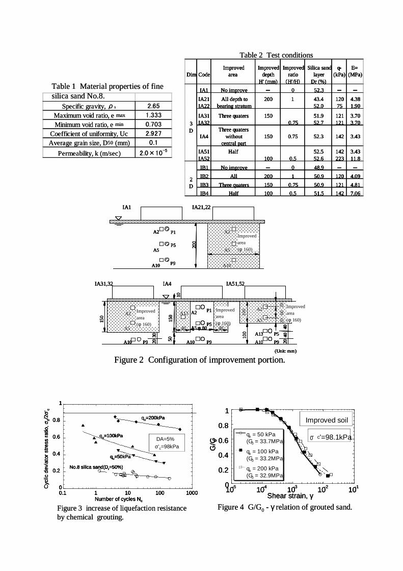
2.2 Test conditions and test procedures Test conditions are summarized in Table 2, and the configurations of improvement portion are

illustrated in Figure 2. 12 centrifuge model tests were conducted. Beside the 2D and 3D conditions, improvement depth (H’) is the main parameter. Four different improvement depth tested were H’/H=0, 1/2, 3/4 and 1. Whole portion underneath the tank to the improvement depth were improved, except IA4 where central portion of three quarters improvement were remained ungrouted.

Unconfined compression strengths of the improved sand were about 120kPa for almost all the cases except of IA22 and IA52, which had about 60% (75kPa) and 160% (223kPa) strengths of the others. Figures 3 and 4 show the results of undrained cyclic triaxial test and the normalized secant shear modulus (G/G0) - shear strain (γ) relation of the grouted sand with various unconfined compression strength respectively. From these two figures it can be confimred that liquefaction resistance of losse sand can be improved by the chmical grouting but not for the small strain stifness.

Centrifuge acceleration employed was 50 g, under which the corresponding prototype is equivalent to a 7m diameter oil tank on 10m depth sand deposit. All tests were carried out by the dynamic geotechnical centrifuge (effective radius: 3.80m, maximum payload: 19.2MN-m/sec2) of Nishimatsu Construction Co., Ltd (Imamura et al., 1998). Input wave for the tests is shown in Figure 5. A sinusoidal wave with acceleration amplitude of 12.5g, frequency of 100Hz (20cycles) was applied to the model for duration of 0.2sec. This input motion is the horizontal acceleration of 250gal, frequency of 2Hz and duration of 10 sec in the prototype scale. Locations of various probes installed in the model are shown in Figure 1 and 2. On measurements, particular attentions were paid to the settlements of ground under the tank base, dynamic responses of the oil tank and excess pore water pressures underneath the soil improvement. Details of the tests are given by Imamura et al. (2004).

3 TEST RESULTS AND DISCUSSIONS 3.1 Variation of observed accelerations with depth in the model

Ratios of observed acceleration amplitude at the tank (A1) and the ground under the tank (A2, A5, A10) to that of the input motion for both 2D and 3D models are shown together with those of surrounding ground (A4, A8, A12) in Figure 6. In all the cases, the ratios are smaller for the shallower depth. As can be seen, there exists a considerable difference between 2D and 3D models. In 3D models, the improvement condition appears to have some influence on the variation of the ratio with the depth. The variations of the ratio in IA4 and IA51 coincide with that in IA1 except of the tank. The variation in IA21 (H’/H=1) was similar to that in IA31 (H’/H=3/4). In general the larger the improvement depth, the smaller the attenuation of the motion. On the other hand, in 2D models all the ratios in the ground with improvement are smaller than those of the case without improving and the difference in the variation of the ratio for different improvement depth is not so clear compared to the 3D models. The variation in the surrounding ground is closer to that under the tank for 2D models than 3D models. This may imply that the end wall effect is more significant in 2D model than 3D

-15

-10

-5

0

5

10

15

0 0.05 0.1 0.15 0.2 0.25

Input wave

Time, (sec)

Acceleration, (g)

Figure 5 Horizontal input motion.

-15

-10

-5

0

5

10

15

0 0.05 0.1 0.15 0.2 0.25

Input wave

Time, (sec)

Acceleration, (g)

Figure 5 Horizontal input motion.

model, because the soil in the surrounding ground is confined by the end wall and the improved soil in 2D model.

In the cases where relatively high ratio was observed below the tank, the ratio of the tank was smaller than that below. As a result, the ratios of the tank are almost the same for all improvement cases. The ratios of the tank under the improved soil are about 40 and 50 % for 2D and 3D models respectively. In the tests the improvement of sand under the tank by chemical grouting did not cause amplification of shaking motion of the tank. 3.2 Settlement under the tank

Figures 7 show the settlements at the center of the tank during shaking. The tank settled with shaking time, but no settlement occurred after shaking except of IA1 which showing small settlement after the shaking. In cases of a half depth improvement in 3D series, settlement rates increased in the middle of shaking time, while for the other cases the settlement rates decreased gradually with time. Maximum settlements normalized by tank diameter (Smax/D) are plotted against soil improvement ratio (V’/V) in Figure 8, where V’ is the volume of the improvement sand, V is that of the cases with entire depth improvement. In Figure 9 improvement efficiency defined by Smax /Smax (NO) are plotted against improvement ratio, where Smax (NO) is the maximum settlement of the case without improvement (IB1 and IA1 for 2D and 3D cases respectively). Tank settlement is effectively reduced by grouting underneath the tank. In 3D series, the tank settlement decrease almost linearly with the improvement ratio for the case with similar strength of grouted sand. In Figures 8 and 9, the results with different strength of the grouted sand (IA22 and IA52) are also plotted. From the figures it can be also confirmed that the strength or stiffness of the grouted sand is also very important for reducing the tank settlement. The higher the strength, the smaller that settlement.

As the stiffness of the active silica gel is not so high, the gradual grouting into sand does not change the stress distribution of the ground underneath the tank. However, once the surrounding ground liquefies, the shear stresses on the vertical surface on the grouted sand diminish, resulting in the concentration of vertical stress on the grouted sand as shown in Figures 10. The concentration of the stress yields the vertical compression of grouted sand. Hence, the stiffness of the sand becomes one of dominant factor of the settlement of grouted sand underneath the tank. IA21 and IA22 were both the entire depth improvement cases, but the settlement in the latter was more than the double of that in the former. This difference can be reasonably explained by smaller E50 in IA22 than IA21 (see Table 2).

0

50

100

150

2000 20 40 60 80 100 120

IB1IB2IB3IB4

Surroundingground

Acceleration amplitude ratio, (%)

2D Model

0

50

100

150

2000 20 40 60 80 100 120

IA1IA21IA31IA41IA51Surroundingground


3D Model

Dep

th (m

m)

Dep

th (m

m)

0

50

100

150

2000 20 40 60 80 100 120

IB1IB2

0

50

100

150

2000 20 40 60 80 100 120

IB1IB2IB3IB4

Surroundingground


2D Model

0

50

100

150

2000 20 40 60 80 100 120



3D Model

Dep

th (m

m)

Dep

th (m

m)

Figure 6 Variation of acceleration amplitude with depth.

0

50

100

150

2000 20 40 60 80 100 120

IB1IB2IB3IB4

Surroundingground


2D Model

0

50

100

150

2000 20 40 60 80 100 120



3D Model

Dep

th (m

m)

Dep

th (m

m)

0

50

100

150

2000 20 40 60 80 100 120

IB1IB2

0

50

100

150

2000 20 40 60 80 100 120

IB1IB2IB3IB4

Surroundingground


2D Model

0

50

100

150

2000 20 40 60 80 100 120



3D Model

Dep

th (m

m)

Dep

th (m

m)

Figure 6 Variation of acceleration amplitude with depth.

0

0.02

0.04

0.06

0.08

0.1

0 0.25 0.5 0.75 1Soil improvement ratio（V'/V）

IA1

IA52(223kPa)

IA51 IA4IA22(75kPa)

IA21

2D

3D

Nor

mal

ized

max

imum

set

tlem

ent :

Sm

ax/D

0

0.02

0.04

0.06

0.08

0.1


IA1

IA52(223kPa)

IA51 IA4IA22(75kPa)

IA21

2D

3D

2D

3D

Nor

mal

ized

max

imum

set

tlem

ent :

Sm

ax/D

Figure 8 Relationship between soil improvement ratio and normalized maximum settlements

0

0.02

0.04

0.06

0.08

0.1


IA1

IA52(223kPa)

IA51 IA4IA22(75kPa)

IA21

2D

3D

Nor

mal

ized

max

imum

set

tlem

ent :

Sm

ax/D

0

0.02

0.04

0.06

0.08

0.1


IA1

IA52(223kPa)

IA51 IA4IA22(75kPa)

IA21

2D

3D

2D

3D

Nor

mal

ized

max

imum

set

tlem

ent :

Sm

ax/D

Figure 8 Relationship between soil improvement ratio and normalized maximum settlements

IA1, IB1

0

0.25

0.5

0.75

1

0 0.25 0.5 0.75 1

IA22(75kPa)

IA52(223kPa)

Soil improvement ratio（V'/V）

IA21

IA4

IA51

IA31

IA32

IB4

IB2IB3

2D3D

S max

/Sm

ax(N

O)

IA1, IB1

0

0.25

0.5

0.75

1

0 0.25 0.5 0.75 1

IA22(75kPa)

IA52(223kPa)


IA21

IA4

IA51

IA31

IA32

IB4

IB2IB3

2D3D

0

0.25

0.5

0.75

1

0 0.25 0.5 0.75 1

IA22(75kPa)

IA52(223kPa)


IA21

IA4

IA51

IA31

IA32

IB4

IB2IB3

2D3D2D3D

S max

/Sm

ax(N

O)

Figure 9 Correlation between soil improvement ratio and improvement efficiency (Smax /Smax (NO)).

IA1, IB1

0

0.25

0.5

0.75

1

0 0.25 0.5 0.75 1

IA22(75kPa)

IA52(223kPa)


IA21

IA4

IA51

IA31

IA32

IB4

IB2IB3

2D3D

S max

/Sm

ax(N

O)

IA1, IB1

0

0.25

0.5

0.75

1

0 0.25 0.5 0.75 1

IA22(75kPa)

IA52(223kPa)


IA21

IA4

IA51

IA31

IA32

IB4

IB2IB3

2D3D

0

0.25

0.5

0.75

1

0 0.25 0.5 0.75 1

IA22(75kPa)

IA52(223kPa)


IA21

IA4

IA51

IA31

IA32

IB4

IB2IB3

2D3D2D3D

S max

/Sm

ax(N

O)

Figure 9 Correlation between soil improvement ratio and improvement efficiency (Smax /Smax (NO)).

Figure 10 Change of stresses in the grouted sand underneath tank due to liquefaction of the .surrounding ground

Before grouting

Stress distribution in the ground

No change in the stress distribution

Shear stress

After grouting

Grouted soil

Liquefaction In ground

Concentration of stress under the tankyields compression of grouted soil

LiquefactionLiquefaction

Reduction of shear stress

Before grouting


Before grouting



Shear stress

After grouting

Grouted soil


Shear stress

After grouting

Grouted soil









Figure 10 Change of stresses in the grouted sand underneath tank due to liquefaction of the .surrounding ground

Before grouting



Shear stress

After grouting

Grouted soil





Before grouting


Before grouting



Shear stress

After grouting

Grouted soil


Shear stress

After grouting

Grouted soil









0

2

4

6

8

100 0.1 0.2 0.3 0.4 0.5

IB1

IB4

IB3 IB2

(a) 2D seriesAt the center of the tank

Time (sec)

Settl

emen

t S

(mm

)0

2

4

6

8

100 0.1 0.2 0.3 0.4 0.5

IB1

IB4

IB3 IB2


Time (sec)

Settl

emen

t S

(mm

)0

2

4

6

8

100 0.1 0.2 0.3 0.4 0.5

IB1

IB4

IB3 IB2


Time (sec)

Settl

emen

t S

(mm

)0

2

4

6

8

100 0.1 0.2 0.3 0.4 0.5

Time (sec)

Set

tlem

ent

S (

mm

)

(b) 3D SeriesAt the center of the tank

IA1

IA4IA51

IA31

IA21

IA520

2

4

6

8

100 0.1 0.2 0.3 0.4 0.5

Time (sec)

Set

tlem

ent

S (

mm

)


IA1

IA4IA51

IA31

IA21

IA52

Figure 7 Settlement at the center of the tank during shaking.

0

2

4

6

8

100 0.1 0.2 0.3 0.4 0.5

IB1

IB4

IB3 IB2


Time (sec)

Settl

emen

t S

(mm

)0

2

4

6

8

100 0.1 0.2 0.3 0.4 0.5

IB1

IB4

IB3 IB2


Time (sec)

Settl

emen

t S

(mm

)0

2

4

6

8

100 0.1 0.2 0.3 0.4 0.5

IB1

IB4

IB3 IB2


Time (sec)

Settl

emen

t S

(mm

)0

2

4

6

8

100 0.1 0.2 0.3 0.4 0.5

Time (sec)

Set

tlem

ent

S (

mm

)


IA1

IA4IA51

IA31

IA21

IA520

2

4

6

8

100 0.1 0.2 0.3 0.4 0.5

Time (sec)

Set

tlem

ent

S (

mm

)


IA1

IA4IA51

IA31

IA21

IA52


0

2

4

6

8

100 0.1 0.2 0.3 0.4 0.5

Time (sec)

Set

tlem

ent

S (

mm

)


IA1

IA4IA51

IA31

IA21

IA520

2

4

6

8

100 0.1 0.2 0.3 0.4 0.5

Time (sec)

Set

tlem

ent

S (

mm

)


IA1

IA4IA51

IA31

IA21

IA52


Three dimensional effect on the tank settlement can be also seen in Figures 8 and 9. The larger settlement and less improvement efficiency were obtained in 3D models than 2D models especially in the cases of a half and three quarters improvements.

Settlement profiles under the tank caused by the shaking are shown in Figures 11. In the case with three quarters depth improvement having no improved portion at the center (IA4), the settlement similar to that of IA21, IA31, about 2mm, took place on the improved portion, but the settlement at the central non-improved portion was about 4mm (60% of IA1). Two main causes of the tank settlement can be considered, one is the volume compression and the other the lateral movement of the soil beneath the tank (Kimura et al. 1995). From the fact explained above, the larger settlement at the central portion can be attributed to the volume compression of non-improved sand within the improved sand. In this test, the base of tank was modelled by rubber membrane to create perfectly flexible condition to avoid the complicated interaction between the tank and soil. However, the settlement at the central portion might be overestimated due to this modelling of tank base compared to the actual tacks with thin steel base plate.

Maximum differential settlements normalized by the tank diameter (δSmax /D) are plotted against the improvement ratio in Figure 12. δSmax /D decreases as the improvement ratio increases, which clearly reveals the efficiency of the improvement. The differential settlement in 3D model is larger than that in 2D, especially for the cases with small improvement ratio. This may be attributed to the high freedom of displacement for 3D condition compared to 2D and the difference of the end wall

0

2

4

6

8

10IB1 IB2 IB3 IB4

-70 -35 0 35 70Position, x, (mm)

2D Model

H’/H=1

H’/H=3/4

H’/H=1/2

H’/H=1

H’/H=3/4

H’/H=1/2

without imp.without imp.

Set

tlem

ent S

(mm

)

0

2

4

6

8

10

IA-1IA-21

IA-31IA-4

IA-51

-70 -35 0 35 70

qu=120～140kPa

Position, x, (mm)

3-D ModelSet

tlem

ent S

(mm

)

qu=120～140kPa0

2

4

6

8

10IB1 IB2 IB3 IB4

-70 -35 0 350

2

4

6

8

10IB1 IB2 IB3 IB4

-70 -35 0 35 70Position, x, (mm)

2D Model

H’/H=1

H’/H=3/4

H’/H=1/2

H’/H=1

H’/H=3/4

H’/H=1/2


Set

tlem

ent S

(mm

)

0

2

4

6

8

10

0

2

4

6

8

10

IA-1IA-21

IA-31IA-4

IA-51

-70 -35 0 35 70

qu=120～140kPaqu=120～140kPa

Position, x, (mm)

3-D ModelSet

tlem

ent S

(mm

)

qu=120～140kPaqu=120～140kPa

Figure 11Settlement profiles under the tank.

0

2

4

6

8

10IB1 IB2 IB3 IB4

-70 -35 0 35 70Position, x, (mm)

2D Model

H’/H=1

H’/H=3/4

H’/H=1/2

H’/H=1

H’/H=3/4

H’/H=1/2


Set

tlem

ent S

(mm

)

0

2

4

6

8

10

IA-1IA-21

IA-31IA-4

IA-51

-70 -35 0 35 70

qu=120～140kPa

Position, x, (mm)

3-D ModelSet

tlem

ent S

(mm

)

qu=120～140kPa0

2

4

6

8

10IB1 IB2 IB3 IB4

-70 -35 0 350

2

4

6

8

10IB1 IB2 IB3 IB4

-70 -35 0 35 70Position, x, (mm)

2D Model

H’/H=1

H’/H=3/4

H’/H=1/2

H’/H=1

H’/H=3/4

H’/H=1/2


Set

tlem

ent S

(mm

)

0

2

4

6

8

10

0

2

4

6

8

10

IA-1IA-21

IA-31IA-4

IA-51

-70 -35 0 35 70

qu=120～140kPaqu=120～140kPa

Position, x, (mm)

3-D ModelSet

tlem

ent S

(mm

)

qu=120～140kPaqu=120～140kPa

Figure 11Settlement profiles under the tank.

0

0.005

0.01

0.015

0.02

2D3D


IA22(75kPa)

IA52(223kPa)

IA1

IA21

IA4

IA51IA31

IA32

Nor

mal

ized

max

imum

diff

eren

tial

settl

emen

t :δS

max

/D

0

0.005

0.01

0.015

0.02

2D3D


IA22(75kPa)

IA52(223kPa)

IA1

IA21

IA4

IA51IA31

IA32

Nor

mal

ized

max

imum

diff

eren

tial

settl

emen

t :δS

max

/D

Figure 12 Relationship between and normalized maximum differential settlements.

0

0.005

0.01

0.015

0.02

2D3D


IA22(75kPa)

IA52(223kPa)

IA1

IA21

IA4

IA51IA31

IA32

Nor

mal

ized

max

imum

diff

eren

tial

settl

emen

t :δS

max

/D

0

0.005

0.01

0.015

0.02

2D3D


IA22(75kPa)

IA52(223kPa)

IA1

IA21

IA4

IA51IA31

IA32

Nor

mal

ized

max

imum

diff

eren

tial

settl

emen

t :δS

max

/D

Figure 12 Relationship between and normalized maximum differential settlements.

effects as discussed before. These comparisons between 2D and 3D models confirm the importance of 3D effects in both physical modelling and numerical modelling on the seismic performance of the tank.

From the observation about the settlements under the tank, it can be concluded that the suppression of vertical and lateral displacements in the area directly beneath the tank by chemical grouting is effective in reducing the settlement and differential settlement of the tank base. In order to establish more rational way for reducing the improvement volume, it is necessary to conduct further tests where the base plate of the tank is properly modeled. 4. CONCLUSIONS

From dynamic centrifuge model tests on efficiency of chemical grouting as a countermeasure against the liquefaction of sand deposits with oil tanks, the following conclusions were drawn. 1. The suppression of vertical and lateral deformation of the area directly beneath the tank by chemical

grouting is effective in reducing both settlement and differential settlements of the tank caused. If the grouted sand has the same stiffness, the maximum and differential settlements decrease almost linearly with the improvement depth.

2. From 2D models qualitatively similar results to 3D models were obtained on the effect of the improvement. However, the maximum and differential settlements were smaller in the 2D models than the 3D models. This may be attributed to the high freedom of displacement for 3D condition compared to 2D and the difference of the end wall effects, which indicating the importance of 3D effects in both physical modelling and numerical modelling on the seismic performance of the tank.

3. If the soil under the central portion of the tank are remained non-improved in order to reduce the volume of the improvement, some differential settlement may take place between improved and non-improved portion. However, the liquefaction of the non-improved sand confined by the surrounding improved sand was effectively prevented. The observed differential settlement in the test might be overestimated due to this modeling of tank base compared to the actual tacks with thin steel base plate.

4. In order to establish more rational way for reducing the improvement volume, it is necessary to conduct further tests where the base plate of the tank is properly modeled.

References: Imamura, S., Hagiwara, T. and Nomoto, T. (1998), “Nishimatsu dynamic geotechnical centrifuge”, Proc. of Centrifuge 98,

25-30. Imamura, S. & Fujii, N. (2002), Observed dynamic characteristics of liquefying sand in a centrifuge, Proc. of Physical

Modeling in Geotechnics, 195-200. Imamura, S, Hirano, T., T. Hagiwara, Takahashi, A. and Takemura, J. (2004), “Centrifuge model tests of exixting oil tanks

on liquefiable loose sand improved by chmical grouting”, Proceeding of JSCE, Geotechnical Division, (to appear). Ishihara, S., Kawase, Y. and Nakajima, M. (1980), “Liquefaction characteristics of sand deposits at an oil tank site during

the 1978 Miyagiken-oki Earthquake, Soils and founda-tions, Vol.20, No.2, pp. 97-111. Kimura, T., Takemura, J., Hiro-oka, A, Okamura, M. and Matsuda, M. ( 1995), “Countermeasures against liquefaction of

sand deposits with structures”, Proc of Earthquake Geo-technical Engineering (edited by Ishihara), IS-Tokyo 95, 1203-1224.

iquefaction remediation of sand with an existing oil …

Documents