ion energization in ganymede’s magnetosphere: using...

Ion energization in Ganymede’s magnetosphere: Using multifluid

simulations to interpret ion energy spectrograms

C. Paty,1 W. Paterson,2 and R. Winglee3

Received 1 October 2007; revised 6 December 2007; accepted 12 February 2008; published 11 June 2008.

[1] We investigate the ion population and energy distribution within Ganymede’smagnetosphere by examining Ganymede’s ionospheric outflow as a source of heavy (O+)and light (H+) ions and the Jovian magnetospheric plasma as an external source ofheavy ions. We develop a method for examining the energy distributions of each ionspecies in a three-dimensional multifluid simulation in a way directly comparable to theobservations of the Plasma Experiment on the Galileo spacecraft. This is used to providenew insight to the existing controversy over the composition of Ganymede’s observedionospheric outflow, and enables further examination of the energetic signatures of the ionpopulation trapped within Ganymede’s magnetosphere. The model-predicted ionosphericoutflow is consistent with the in situ ion energy spectrograms observed by the GalileoPlasma Experiment at closest approach, and requires that both ionospheric H+ and O+ arepresent in the population of ions exiting Ganymede’s ionosphere over the polar cap. Theoutward flux of ionospheric ions was calculated to be ~1026 ions/cm2/s, which is inagreement with independently calculated sputtering rates of Ganymede’s icy surface. Themodeled spectrograms define characteristic energy signatures and populations forvarious regions of Ganymede’s magnetosphere, which illustrate the major sources of ionstrapped within the magnetosphere are Ganymede’s ionospheric O+ and H+. The fact thatvery little plasma was observed inside Ganymede’s magnetosphere during the G8 flyby isattributed to the region being shadowed from the sun for ~60 h, which may indicatethe importance of photoionization for sustaining Ganymede’s ionospheric plasma source.

Citation: Paty, C., W. Paterson, and R. Winglee (2008), Ion energization in Ganymede’s magnetosphere: Using multifluid

simulations to interpret ion energy spectrograms, J. Geophys. Res., 113, A06211, doi:10.1029/2007JA012848.

1. Introduction

[2] In order to understand the plasma population andenergy distribution in Ganymede’s magnetosphere it isimportant and necessary to account for the various sourcesof plasma into the system. Previously, researchers have usedresistive magnetohydrodynamic (MHD) simulations tostudy Ganymede’s magnetosphere [Stone and Armstrong,2001; Kopp and Ip, 2002; Ip and Kopp, 2002]. However,those studies focused on the effects of variations in theincident Jovian magnetic field orientation on Ganymede’smagnetic morphology and did not incorporate the variousion sources responsible for the observed plasma dynamicperturbations to the magnetic field [cf. Kivelson et al.,1998]. Multifluid simulations enable us to track multipleion species from different sources as they propagate throughthe simulation space and interact with electric and magnetic

fields. Comparative studies between 3D multifluid simula-tions and Galileo magnetometer data were performed inorder to develop a quantitative model of the currents andfields within Ganymede’s magnetosphere [Paty andWinglee,2004, 2006]. The multifluid model demonstrated goodagreement with the Galileo magnetometer observations ofthe strength and structure of Ganymede’s magnetosphere foreach of the six flybys.[3] The plasma population of Ganymede’s near space

environment has been a source of much debate. The PlasmaExperiment on the Galileo spacecraft was designed toobserve the low energy plasma population, ranging fromas low as ~1 eV up to ~50 keV; a complimentary andslightly overlapping range when compared to the EnergeticParticle Detector (EPD). It had the capacity to measure thetemperature, density and bulk motion of the low energy ionsand electrons. The Plasma Experiment not only character-ized the low energy plasma of the Jovian magnetosphere,but was pivotal in observing the polar ionospheric outflowat Ganymede [Frank et al., 1997]. However, the composi-tion of the outflowing ion population can not be directly oruniquely inferred from the observed ion energy spectro-grams. Frank et al. [1997] interpreted the cold population ofions flowing out of the polar cap as H+. Vasyliunas andEviatar [2000] developed a different interpretation wherethey determined the composition of the cold outflow could

JOURNAL OF GEOPHYSICAL RESEARCH, VOL. 113, A06211, doi:10.1029/2007JA012848, 2008

1Space Science and Engineering Division, Southwest Research Institute,San Antonio, Texas, USA.

2Center for Atmospheric Sciences, Hampton University, Hampton,Virginia, USA.

3Department of Earth and Space Sciences, University of Washington,Seattle, Washington, USA.

Copyright 2008 by the American Geophysical Union.0148-0227/08/2007JA012848

A06211 1 of 10

be O+. An O+ outflow was somewhat more consistent withthe atmospheric models of Eviatar et al. [2001] but did notexplain the observed Lyman alpha airglow emissions indi-cating a hydrogen exosphere [Barth et al., 1997].[4] This study looks to further our understanding of how

Ganymede’s magnetosphere interacts with the Jovian mag-netosphere through the use of multifluid simulations whichcan describe and account for the Galileo Plasma Experimentobservations. Three dimensional multifluid simulations ofGanymede’s magnetosphere were performed, and a methodfor direct comparison between the modeled ion energyenvironment and the ion energy distributions observed bythe Galileo spacecraft was developed. Ion species sourcedfrom the Jovian magnetosphere and from Ganymede’sionosphere were tracked in order to calculate their fluxesinto and out of the system and to determine their relativeimportance to the composition and energy budget of Gany-mede’s magnetosphere. This enabled further interpretationof the observed ion energy spectrograms and gave newinsight to the ionospheric outflow debate.

2. Methods

2.1. The Multifluid Model and Boundary Conditions

[5] A 3D multifluid model was used to examine themagneto-plasma interactions of Jupiter and Ganymede’smagnetospheres local to Ganymede. Multifluid simulationsexplicitly track the various ion species, which enablesexamination of differential heating and acceleration of eachion species. They also allow us to determine which ionsources make up the population of a given region of thesimulation. The multifluid treatment, explained at length forthe context of Ganymede magnetospheric simulations byPaty and Winglee [2006], keeps track of the different ionspecies as separate fluids for which the ion gyromotion isnot averaged out. This model uses a high resolution nestedgrid, which makes it possible to resolve the acceleration anddrift motion associated with the ion gyromotion. The inner-most box has a resolution of 0.45 RG or about 120 km, andextends from approximately �3 to 3 RG in x, �2 to 2 RG iny and �2 to 2 RG in z. The simulation has a grid spacingthat increases by a factor of two between consecutive boxes,with the largest simulation volume of dimension 48 RG in xand 32 RG in y and z. A Cartesian coordinate system isused, where x is defined to be in the flow direction of theJupiter’s corotational velocity at Ganymede, y points inthe Ganymede-to-Jupiter look direction, and z is along therotational axis of Ganymede (GPHIO coordinates). A de-tailed comparison of the multifluid model to hybrid simu-lations found that the ion drift motion due to explicitlymodeled gyromotion in the hybrid case was comparable tothe ion drift motion in the multifluid treatment [Harnett et al.,2005].[6] The ions that populate Ganymede’s magnetosphere

come from two sources: the incident Jovian magnetospheric

plasma (JMP) and Ganymede’s ionosphere. The boundaryconditions used in the model for these parameters aredescribed in detail by Paty and Winglee [2006]. In brief,the JMP is composed of plasma from the Io plasma torus,Jupiter’s ionosphere, and to a much lesser extent the solarwind. We chose to model the major constituents of the JMP(mostly O+ and a few percent H+) as determined byupstream observations [Frank et al., 1997; Neubauer,1998]. The Jovian magnetic field strength and orientationand the JMP Mach numbers for the three flyby encounters(G2, G7, and G8) studied in the paper were determinedfrom unperturbed spacecraft observations before and afterthe encounter [Neubauer, 1998; Kivelson et al., 2002] andare listed in Table 1.[7] Ganymede’s ionosphere base was set with a density of

5200 ions/cm3, with a 4:1 ratio of O+ to H+ ions, and a scaleheight of 125 km based on the chemical models of Eviatar etal. [2001], sputtering rates of Ip et al. [1997] andParanicas etal. [1999], and sputtering products of Herring-Captain et al.[2005]. The ionospheric ions at the inner boundary wereprescribed temperatures that ranged smoothly from 6.0 to0.1 eV for the equatorial to polar regions, respectively. Theionospheric density at the inner boundary was held constanton the assumption of a constant source of ionosphericmaterial [Ip et al., 1997; Paranicas et al., 1999], and thebase of the ionosphere was given a resistivity of 3800 Wm toaccount for collisions. Everywhere else in the simulation theresistivity was set to zero, corresponding to the collisionlessplasma environment at Ganymede. In this model we use threeion fluids: the ionospheric O+, which is tracked separatelyfrom the JMP O+, and an H+ fluid that combines the iono-spheric H+ and the few percent JMP H+. The H+ fluid will bereferred to as ionospheric H+ for simplicity as it onlyrepresents a few percent of the JMP.

2.2. Generating Synthetic Ion Energy Spectrograms

[8] In order to determine the energy distributions for eachion species in the simulation for this comparison, thedensity, temperature, and velocity for each ion specieswas sampled along the coordinates of a given Galileo flyby.Assuming a Maxwellian distribution for the ions, a proba-bility distribution was determined over an energy (E) rangeof 10 eV to 105 eV (100 keV) to correspond to thesensitivity range of the Plasma Experiment such that

Pi E; xð Þ ¼ e� V E;mið Þ�Vi xð Þð Þ2= 2VTi xð Þ2ð Þð Þ

VTi xð Þ3 2�ð Þ3=2: ð1Þ

Here x corresponds to positions along the spacecrafttrajectory, VTi is the ion thermal velocity at each location(x) along the trajectory, and Vi is the magnitude of the ionvelocity at each location. V is the velocity that correspondsto the energy in the range being integrated over and themass of each ion species (mi) such that

V E;mið Þ ¼ffiffiffiffiffiffi2E

mi

r: ð2Þ

To obtain the flux of particles per electron volt (Ni), whichis in units of ions/s/eV/cm2, the probability distribution wasmultiplied by the number density for each ion and the

Table 1. Upstream Magnetic Field Observations Near Ganymede

Flyby Bx, nT By, nT Bz, nT MVA MVS

Location Relativeto Plasma Sheet

G2 17.0 �72.9 �84.7 0.50 1.8 aboveG7 �3.00 83.7 �75.6 0.50 1.8 belowG8 �11.0 11.0 �77.6 1.00 1.8 inside

A06211 PATY ET AL.: ION ENERGIZATION AT GANYMEDE

2 of 10

A06211

square of the velocity V, and divided by the ion mass. Thisexpression

Ni E; xð Þ ¼ ni xð ÞV E;mið Þ2

mi

� Pi E; xð Þ

¼ 1

2pð Þ3=21

miVTi xð Þ2ni xð ÞV E;mið Þ2

VTi xð Þ

� e� V E;mið Þ�Vi xð Þð Þ2= 2VTi xð Þ2ð Þð Þ ð3Þ

can then be summed over all the ion species to obtain anenergy spectrogram that is directly comparable to theobservation of the Galileo Plasma Experiment, or it can beplotted separately to examine the contribution of each ionspecies to the net energy distribution.

3. Results

3.1. Tracking Ion Sources

[9] In tracking the motion of these ion species as thesystem evolves toward steady state, the model demonstratedthat Ganymede’s magnetic field provides shielding frommost of the bulk flow of the JMP. This leads to Ganymede’smagnetosphere being primarily populated by Ganymede’sionospheric constituents. Figure 1 details the density distri-bution for each of the three modeled ion species throughoutthe system. In Figure 1 the first row illustrates the mor-phology of the magnetic field at Ganymede as it encountersthe Jovian plasma in Jupiter’s magnetospheric lobe as wellas the density of each of the three modeled ion species in thex-z and x-y planes. Note that the color bar is consistent forall of the plots. At equatorial latitudes the bulk flow of theJMP is almost completely excluded from Ganymede’smagnetosphere. Some of the bulk flow of the JMP on theflow facing side can gain access to Ganymede’s ionosphereand surface through the cusps [Paty and Winglee, 2004].Ganymede’s ionospheric H+ and O+ dominate the compo-sition of Ganymede’s magnetosphere, though the iono-spheric O+ is higher in density than the ionospheric H+.Note that this O+ dominance is a reflection of the 4:1 ratioof O+ to H+ at the ionospheric boundary.[10] The second row in Figure 1 shows the ion density for

each species, as well as the flow velocities projected in the x-zplane. The arrows show the direction of the flow and the sizeof the arrows scale relative to the magnitude of the velocityfor each species. The deflection of the JMP in the upstreamregion where it approaches Ganymede’s magnetopause isclearly illustrated. The convection of JMP over the poles anddown tail can be seen along with the flow of the ionosphericH+ andO+ ions out of the poles being convected down tail. Asthe magnetic fields in the tail reconnect, the ion flow isredirected along closed field lines back toward Ganymede. Itis through this process that the JMP gains access to Gany-mede’s magnetotail and a fraction of the polar ionosphericoutflow of O+ and H+ ions is trapped into populatingGanymede’s magnetosphere. The H+ ion velocities trackclosely with the boundary between open and closed fieldlines leading to the tail reconnection region, while the heavyspecies flow down-tail and are redirected near the equatorialplane. This phenomenonwas also noted by Shay and Swisdak[2004] when modeling the effects of the presence of heavyions on reconnection.

[11] In row three the view is shifted to look down uponthe equatorial plane and show the density and flow for eachmodeled ion species. Again the deflection of the upstreamJMP is noticeable as the vectors indicate the motion of theflow around Ganymede’s magnetosphere. Ganymede’s flowfacing magnetosphere shields out the bulk JMP flow in theequatorial plane. In the magnetotail region the JMP gainsaccess through reconnection and the flow of JMP appearsquite asymmetric. Down-tail flows of JMP on the anti-Jupiter flank of the magnetotail are shown directly next todistinct inward moving flows. The inward transport of JMPtapers in magnitude as you move across the magnetotail inthe y-direction as well as in the negative x direction wherethe JMP stops short of convecting completely into the innermagnetosphere from down-tail. Asymmetries in the equa-torial magnetotail are visible in the ionospheric H+ and O+

as well, and are due to the ion cyclotron motion and finiteLarmor radius effects. The mass difference between theionospheric H+ and O+ makes the O+ Larmor radius a factorof 16 larger than that of H+, and is responsible for thedifferences in flow and density asymmetries in the equato-rial flow figures. For example, the heavy ionospheric ions inthe tail are deflected in the negative y-direction, an effectquite noticeable in the O+ but not significant in the H+

ionospheric ions. Such flow and density asymmetries be-tween heavy and light ions have been shown in hybridmodels for other moons [Simon et al., 2007] but would notbe present in an ideal MHD model where the ion cyclotronmotion is averaged out and the ions and electrons arecollapsed into a single fluid.

3.2. Interpreting Ionospheric Outflow

[12] In order to better understand the flow of ionosphericions away from Ganymede, the net flux of each ion specieswas determined. The flux of the ionospheric H+ and O+ ionswas calculated at a distance of 24 RG in order to determinethe amount of ionospheric ions lost from the system andpicked up by the Jovian magnetosphere. This ensured thatthe flux was determined further down the magnetotail thanthe location of reconnection (which occurs at ~7 RG, ± 2 RG

as upstream conditions vary), and that the ions flowing outof the system would not become trapped on newly closedfield lines and be redirected back toward Ganymede. At24 RG it was calculated that Ganymedewas losing on average4 � 1026 ions/s of ionospheric O+ and 1 � 1026 ions/s ofionospheric H+. The 4:1 ratio in the fluxes of O+ andH+ beingdirectly linked to the choice of the ionospheric composition atthe inner boundary.[13] The flux of ionospheric H+ and O+ was also deter-

mined near the surface of Ganymede, at a distance of 3 RG.The factor of ~4 difference between the rate of O+ and H+

ions flowing out of Ganymede’s ionosphere was stillpresent, however some of the outflow at this distance wouldbecome trapped in Ganymede’s magnetosphere. The differ-ence in outflow rates is evident when examining the ionpopulation of Ganymede’s magnetosphere in the first row ofFigure 1. Here the ionospheric O+ density is shown to be thedominant species in Ganymede’s magnetosphere by a factorof 2 to 8, with the highest density ratios occurring alongclosed field lines. Since the ionospheric outflow suppliesGanymede’s magnetosphere with plasma, the difference in


3 of 10

A06211

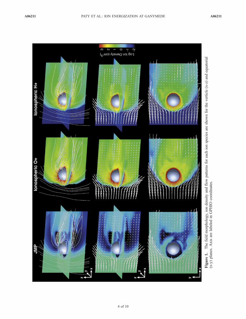
Figure

1.

Thefieldmorphology,iondensity

andflowpatternsforeach

ionspeciesareshownfortheverticle(x-z)andequatorial

(x-y)planes.Axisarelabeled

inGPHIO

coordinates.


4 of 10

A06211

the outflow rates of O+ and H+ is represented in the iondensity distribution.[14] While the net ionospheric loss was calculated to be

on average 1 � 1026 and 4 � 1026 ions/s of H+ and O+ ionsrespectively, these values were variable depending on thelocation of Ganymede with respect to the Jovian plasmasheet. In the Jovian plasma sheet, where the magnetic fieldstrength is weaker, we see a drop in the ionospheric outflowby a factor of 2 relative to when Ganymede resides outsidethe Jovian plasma sheet. The average ionospheric outflowrate from the simulations can be compared to the sputteringrate independently determined from observations made bythe Energetic Particle Detector and Plasma Experiment onGalileo. Paranicas et al. [1999] determined that the sputter-

ing rate should be ~2 � 1026 water molecules/s in agree-ment with calculations by Ip et al. [1997]. Hence themultifluid simulations produce ionospheric outflows thatare consistent with the sputtering rate assumed to supply thebase of the ionosphere in the model.[15] JMP ions lost to Ganymede were also calculated for

the simulation, with ~2 � 1026 ions/s passing into theionosphere. This value varies by nearly an order of magni-tude depending on where Ganymede is located relative tothe Jovian plasma sheet, with fluxes as small as 5 � 1025 inthe lobe. The JMP density is higher and its gyroradius largerin the Jovian plasma sheet relative to in the lobes; thesecharacteristics are responsible for the higher fluxes of JMPto Ganymede’s surface while its orbit resides in the plasmasheet. This bulk flux into Ganymede is important for itdrives processes like sputtering, excitation of aurora andairglow. We do not expect this number to be exactlybalanced by the net ionospheric loss rate, since not allsputtering products are lost or even populate the ionosphere.A fraction of sputtering related products recombines andprecipitates back to the surface as a water frost layer. Inaddition, processes like sputtering and aurora can be drivenby electron precipitation and the precipitation of the ener-getic tails of the ion distributions not incorporated in theabove flux calculation. Keep in mind that ions and electronsthat pass into the ionosphere are lost to the simulation; thephysics and chemistry associated with generating aurora,dissociation, ion-neutral interactions, and surface sputteringare not yet included in the formulation driving the simulation.

3.3. Energy Distribution in Ganymede’sMagnetosphere

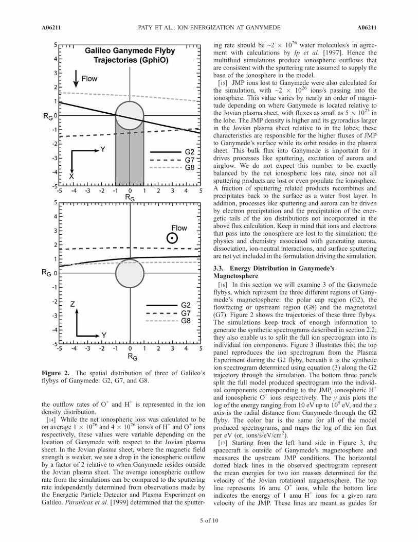
[16] In this section we will examine 3 of the Ganymedeflybys, which represent the three different regions of Gany-mede’s magnetosphere: the polar cap region (G2), theflowfacing or upstream region (G8) and the magnetotail(G7). Figure 2 shows the trajectories of these three flybys.The simulations keep track of enough information togenerate the synthetic spectrograms described in section 2.2;they also enable us to split the full ion spectrogram into itsindividual ion components. Figure 3 illustrates this; the toppanel reproduces the ion spectrogram from the PlasmaExperiment during the G2 flyby, beneath it is the syntheticion spectrogram determined using equation (3) along the G2trajectory through the simulation. The bottom three panelssplit the full model produced spectrogram into the individ-ual components corresponding to the JMP, ionospheric H+

and ionospheric O+ ions respectively. The y axis plots thelog of the energy ranging from 10 eV up to 105 eV, and the xaxis is the radial distance from Ganymede through the G2flyby. The color bar is the same for all of the modelproduced spectrograms, and maps the log of the ion fluxper eV (or, ions/s/eV/cm2).[17] Starting from the left hand side in Figure 3, the

spacecraft is outside of Ganymede’s magnetosphere andmeasures the upstream JMP conditions. The horizontaldotted black lines in the observed spectrogram representthe mean energies for two ion masses determined for thevelocity of the Jovian rotational magnetosphere. The topline represents 16 amu O+ ions, while the bottom lineindicates the energy of 1 amu H+ ions for a given ramvelocity of the JMP. These lines are meant as guides for

Figure 2. The spatial distribution of three of Galileo’sflybys of Ganymede: G2, G7, and G8.


5 of 10

A06211

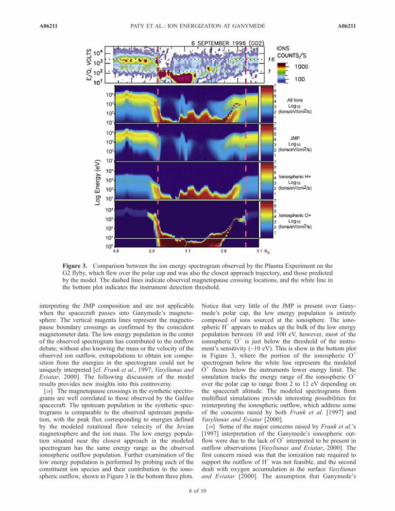
interpreting the JMP composition and are not applicablewhen the spacecraft passes into Ganymede’s magneto-sphere. The vertical magenta lines represent the magneto-pause boundary crossings as confirmed by the coincidentmagnetometer data. The low energy population in the centerof the observed spectrogram has contributed to the outflowdebate; without also knowing the mass or the velocity of theobserved ion outflow, extrapolations to obtain ion compo-sition from the energies in the spectrogram could not beuniquely interpreted [cf. Frank et al., 1997; Vasyliunas andEviatar, 2000]. The following discussion of the modelresults provides new insights into this controversy.[18] The magnetopause crossings in the synthetic spectro-

grams are well correlated to those observed by the Galileospacecraft. The upstream population in the synthetic spec-trograms is comparable to the observed upstream popula-tion, with the peak flux corresponding to energies definedby the modeled rotational flow velocity of the Jovianmagnetosphere and the ion mass. The low energy popula-tion situated near the closest approach in the modeledspectrogram has the same energy range as the observedionospheric outflow population. Further examination of thelow energy population is performed by probing each of theconstituent ion species and their contribution to the iono-spheric outflow, shown in Figure 3 in the bottom three plots.

Notice that very little of the JMP is present over Gany-mede’s polar cap, the low energy population is entirelycomposed of ions sourced at the ionosphere. The iono-spheric H+ appears to makes up the bulk of the low energypopulation between 10 and 100 eV, however, most of theionospheric O+ is just below the threshold of the instru-ment’s sensitivity (~10 eV). This is show in the bottom plotin Figure 3, where the portion of the ionospheric O+

spectrogram below the white line represents the modeledO+ fluxes below the instruments lower energy limit. Thesimulation tracks the energy range of the ionospheric O+

over the polar cap to range from 2 to 12 eV depending onthe spacecraft altitude. The modeled spectrograms frommultifluid simulations provide interesting possibilities forreinterpreting the ionospheric outflow, which address someof the concerns raised by both Frank et al. [1997] andVasyliunas and Eviatar [2000].[19] Some of the major concerns raised by Frank et al.’s

[1997] interpretation of the Ganymede’s ionospheric out-flow were due to the lack of O+ interpreted to be present inoutflow observations [Vasyliunas and Eviatar, 2000]. Thefirst concern raised was that the ionization rate required tosupport the outflow of H+ was not feasible, and the seconddealt with oxygen accumulation at the surface Vasyliunasand Eviatar [2000]. The assumption that Ganymede’s

Figure 3. Comparison between the ion energy spectrogram observed by the Plasma Experiment on theG2 flyby, which flew over the polar cap and was also the closest approach trajectory, and those predictedby the model. The dashed lines indicate observed magnetopause crossing locations, and the white line inthe bottom plot indicates the instrument detection threshold.


6 of 10

A06211

ionosphere is composed almost entirely of O+ and O2+ ions

comes from the hypothesis that sputtering of surface ice anddissociation of water group molecules imparts enoughenergy on neutral H and H2 that it escapes before becomingionized [Eviatar et al., 2001], hence the concern over Franket al.’s [1997] identification of the outflow as H+. However,recent laboratory studies have demonstrated that surfacesputtering may produce more H+ and H2

+ than initiallythought [Herring-Captain et al., 2005], especially at thelow temperatures present on Ganymede’s surface. Thesecond concern stated that if the outflow consisted of H+

ions it would leave behind an accumulation of meters ofoxygen on the surface, a feature not found in any surfacespectral analysis. Vasyliunas and Eviatar [2000] argue thatto solve both of these concerns the outflow populationshould be reinterpreted as a low energy population of O+,moving at a quarter of the speed noted for the H+ interpre-tation. This would keep with the observed energy range ofthe outflow population, solve the H+ ionization rate issueand make sure that meters of oxygen were not left accu-mulating on Ganymede’s surface.[20] However, the idea that O+ could be flowing out of

Ganymede’s polar ionosphere at energies just below thethreshold of the Plasma Experiment was not considered.

The model predicts that O+ ions are accelerated to energiesof 3 to 12 eV over the polar cap (at G2 flyby altitudes),energies just at or below the detection threshold of thePlasma Experiment. H+ ions from the ionosphere reachenergies of 10 to 100 eV at the same altitudes and underthe same model conditions. With this in mind, an alternateinterpretation of the Plasma Experiment observation ispresented. The ionosphere over Ganymede’s polar cap,assumed to be composed of mostly O+ ions and some H+

ions, produces an ionospheric outflow of H+ and lowerenergy O+. The number fluxes of these species werecalculated in the previous section, and it was determinedthat their relative abundance in the ionosphere was propor-tional to their relative outflow rates. While it appearsnecessary to have a measurable H+ component in Gany-mede’s ionosphere to account for the ion energies observedby the Plasma Experiment, the ratio of H+ relative to O+ isnot well constrained. More research is currently underwayto determine to relative abundance of H+ in Ganymede’sionosphere resultant from direct ionization from energeticparticle interactions with the icy surface. However, regard-less of the exact composition, the presence of a strong O+

ionospheric population is generally agreed upon [Eviatar etal., 2001; Cooper et al., 2001] and the outflow of iono-

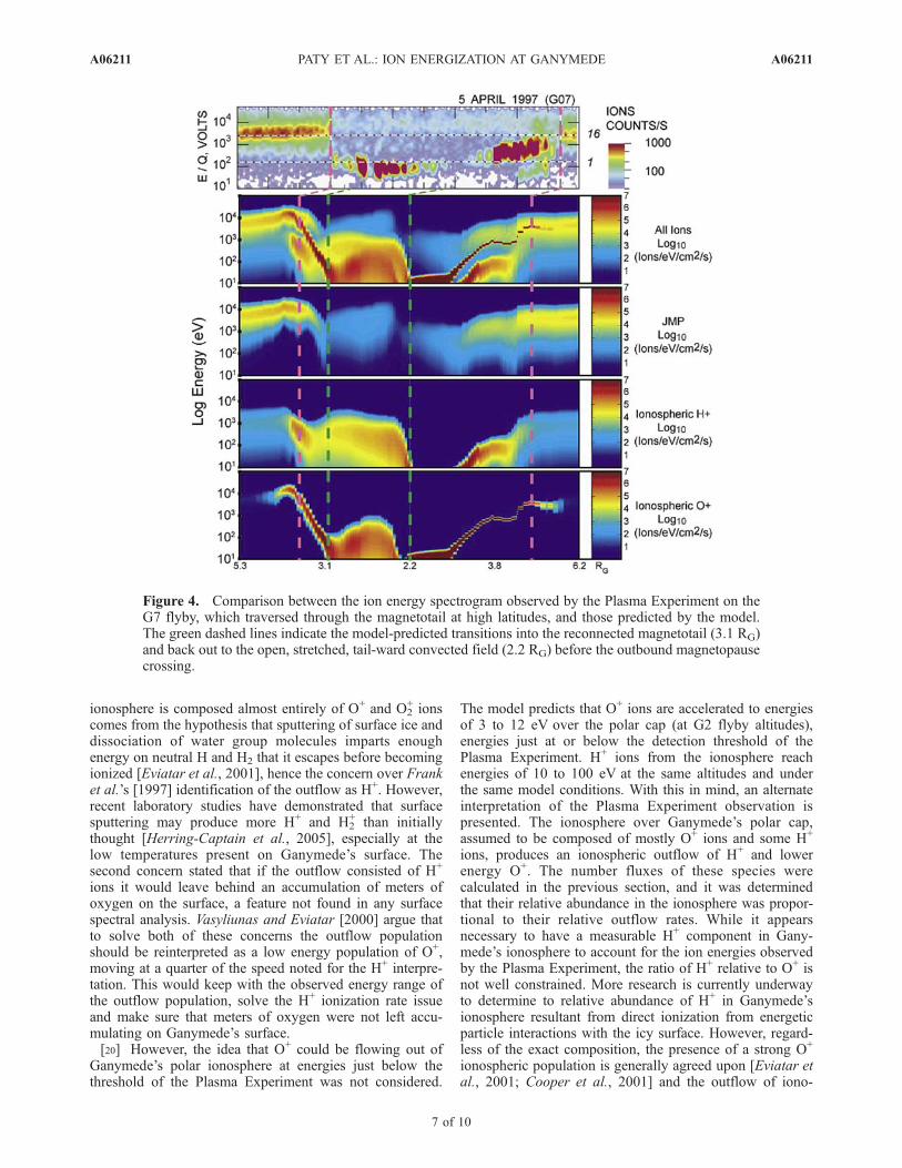
Figure 4. Comparison between the ion energy spectrogram observed by the Plasma Experiment on theG7 flyby, which traversed through the magnetotail at high latitudes, and those predicted by the model.The green dashed lines indicate the model-predicted transitions into the reconnected magnetotail (3.1 RG)and back out to the open, stretched, tail-ward convected field (2.2 RG) before the outbound magnetopausecrossing.


7 of 10

A06211

spheric O+ helps in addressing the issue of oxygen buildingup on Ganymede’s surface. H+ may be escaping in theobservable range of 10 to 100 eV, but O+ is also obtainingenergies corresponding to velocities greater than escape

velocity of 2.74 km/s, where vescape =ffiffiffiffiffiffiffiffiffiffi2GMG

RG

q. Hence

oxygen is likely not building up on Ganymede’s surface;it is escaping at energies just below the detection range ofthe Plasma Experiment.[21] Another way to test the accuracy of the modeling is

to undertake a comparative study with the data from otherflybys. Figure 4 compares the observed ion energies fromthe G7 (magnetotail) flyby to those derived from the modelalong the same trajectory, while Figure 5 compares theobservations and model predictions from the flow facingmagnetosphere flyby (G8) (cf. Figure 2 for flyby locations).It is first evident when comparing the G7 (Figure 4) and G8(Figure 5) Plasma Experiment observations that the ionenergy distributions are significantly different in the mag-netotail versus on the flow facing side. The ions in Gany-mede’s magnetotail (Figure 4) are observed to have muchhigher energies than the trapped ions in the flow facingmagnetosphere. In the G7 flyby, the spacecraft crosses themagnetopause boundary at approximately 3.1 RG, indicatedby the dashed magenta line in Figure 4. The ion energydistribution changes significantly after the crossing; the bulkenergy at the peak flux drops to ~100 eV. There is a shortdropout in the flux near closest approach, after which the

ions increase in energy as the spacecraft approaches theoutbound magnetopause crossing. A second population isnoticeable at lower energies during the outbound portion ofthe flyby, before the spacecraft passes back into the Jovianmagnetosphere.[22] The structure in the energy distribution in Gany-

mede’s tail is mostly predicted by the simulation and shownin the bottom panels of Figure 4. The duration the spacecraftspends within the magnetotail is well predicted by themodel, as is the general morphology of the energy distri-bution within the magnetopause crossings. Both the ob-served spectrogram and the modeled spectrogram inFigure 4 show a relatively small flux of keV ions insideGanymede’s magnetosphere. This diffuse population is atenergies near those of the incident JMP, and by separatingout the ion species (bottom three panels of Figure 4) themodel indicates that the composition is in fact sourced fromthe JMP. This diffuse population is present in all threeflybys presented here, but was most noticeable in theGalileo data in the high latitude wake flyby (G7). In theoutbound portion of the flyby two ion populations areclearly visible; the ratio of their mean energies correspondsapproximately to a factor of 16 difference in mass indicatingthat they are moving at the same velocity. Again, decom-posing the modeled spectrogram into the constituent ionspecies, it becomes apparent that both populations aresourced from Ganymede’s ionosphere.

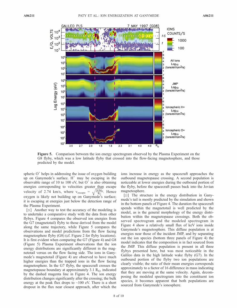
Figure 5. Comparison between the ion energy spectrogram observed by the Plasma Experiment on theG8 flyby, which was a low latitude flyby that crossed into the flow-facing magnetosphere, and thosepredicted by the model.


8 of 10

A06211

[23] The main noticeable difference between the observedand the model predicted spectrograms is that the predictedspectrogram shows the spacecraft passing into the closedfield region of Ganymede’s magnetotail between 3.1 and 2.2RG, the area between the dashed green lines in Figure 4. Theclosed field line interpretation for this region of the modelcomes from combining 3-dimensional renderings (similar tothose in Figure 1, but for the G7 flyby conditions) and thesynthetic spectrogram technique. The descending energyregion directly after the magnetopause crossing in themodeled G7 flyby can be interpreted as the spacecraftencountering Ganymede’s open field lines which arestretching tail-ward. The spacecraft then passes into thereconnected magnetotail (at the first green dashed line inFigure 4), where the ions have been heated as illustrated bythe broadened energy distributions between the greendashed lines. The observed spectrogram does not appearto show the spacecraft passing into the closed field lineregion. This is confirmed by further examination of theplasma data. During the G7 encounter the flow of ions wasuniformly tailward, an observation confirmed by the factthat the cold ions in the spectrogram only appear in sensorsP6 and P7 (the spectrograms presented in the paper averageover all of the sensor look directions). This uniform tailwardflow is inconsistent with the spacecraft flying throughclosed field lines in the tail.[24] The discrepancy between the observed and modeled

spectrograms is due to the fact that the size and shape of themagnetotail is highly susceptible to the upstreamflow con-ditions of Jupiter’s rotating magnetosphere which variesthroughout the flyby as Jupiter’s plasma sheet wobbles overGanymede’s orbital location [cf. Kivelson et al., 2002]. Thesimulation is run to a quasi-steady state with the upstreamconditions held constant, which could account for the slightdiscrepancy between the morphology of the modeled andthe observed magnetotail. By shifting the spacecraft loca-tion 1 grid space in the +Z direction in the simulation, wefind that it does not encounter the closed field line region.One grid space is equivalent to 0.045 RG, which demon-strates how slight the difference is between the modeled andobserved morphology of Ganymede’s magnetosphere. Also,mapping the spacecraft trajectory onto Cartesian grid hasinherent uncertainty since modeled quantities are explicitlycalculated on the grid point, hence a difference on of 1 gridspace in mapping the trajectory is reasonable within theuncertainty of this method.[25] The energy distribution observed on the flow facing

part of Ganymede’s magnetosphere was much different thanthat observed in the magnetotail (or wake) region. Figure 5compares the G8 Plasma Experiment observation, whichoccurred on the upstream side of Ganymede at low lat-itudes, to model predicted energy spectrograms in the samemanner as Figures 4 and 5. The spacecraft observedenhancements in the ion counts per second around thekeV energy range directly after crossing into Ganymede’smagnetosphere and just before exiting, likely the result ofmoving through Ganymede’s magnetosheath. The centralregion of the spectrogram, which corresponds to the space-crafts closest approach to Ganymede and is located wellwithin Ganymede’s magnetosphere, shows almost no ioncounts in the >100 eV energy range. There appears to besome flux in the range of 10 to 100 eV near closest

approach (~1.6 RG), however that borders on the lowerlimit of the instruments sensitivity.[26] In themodeled spectrogram (second panel in Figure 5),

there is a significant ion signature between the magnetopausecrossings. In the bottom three panels it is shown that themodeled signature at closest approach is representative ofionospheric H+ and O+ ions trapped along closed field linesin Ganymede’s magnetosphere. The energy of the iono-spheric O+ in this region is at higher energies than theionospheric H+, and the ratio of energies implies that theyhave similar velocities. The lack of ions near closest ap-proach in the observation is not reproduced in the simula-tion. While the model predicts the location, energies anddensities of multiple ion species, it does not take into accountthe chemistry corresponding to photoionization and recom-bination in Ganymede’s ionosphere. At the time of the G8flyby, the upstream hemisphere had been shadowed from thesun for ~40 h, hence much of its ionosphere would haverecombined causing the dropout of ions observed at closestapproach. The model did not incorporate such ionosphericasymmetries as it had not been reported in the literature orexisting ionospheric models for Ganymede. The modelshould accurately depict the ion energy distribution at lowlatitudes in a sunlit upstream magnetosphere, however nosuch flyby exists in the six performed by Galileo forcomparison. The observation combined with the modelprediction raises new questions regarding the importanceof photoionization for Ganymede’s atmosphere and iono-sphere, the effects of which may also be noticeable in the G2flyby (cf. Figure 3, top panel). The ion signature measure-ments after closest approach during the G2 flyby aresubstantially weaker than those from the inbound portionof the flyby. The weaker particle fluxes correspond to theGalileo spacecraft crossing the terminator into the shadednight-side region in the outbound portion of the flyby, wherephotoionization would not contribute to the ionosphericdensity.

4. Conclusions

[27] This paper addressed the ion population, ionosphericoutflow and ion energy distributions within Ganymede’smagnetosphere. In order to understand the plasma popula-tion and distribution within Ganymede’s magnetosphere, itwas important to account for the various sources of plasmainto the system. While Ganymede’s magnetosphere is smallin size and strength relative to the magnetic field of therotating Jovian magnetosphere, it still provides enoughshielding to exclude much of the JMP at low latitudes(<45�). The JMP gains access through two processes: someprecipitates through Ganymede’s cusps and some convectsdown tail and becomes trapped along reconnected fieldlines. Ganymede’s magnetospheric plasma is composed ofmostly ionospheric O+ and H+ ions. These ions originate inthe ionosphere, flow out at the polar cap regions, areconvected down tail and a fraction of the outflow iseventually trapped on reconnected field lines. The escapingflux rate of the ionospheric O+ and H+ was calculated to beon the order of 1026 ions/s for the simulation, which is wellcorrelated to the independently determined sputtering ratefor the surface of Ganymede that actively supplies the


9 of 10

A06211

atmosphere and ionosphere [Ip et al., 1997; Paranicas etal., 1999].[28] While examining the density distribution and flow of

ions was useful for understanding how various ion speciespopulate different regions of Ganymede’s near space envi-ronment, it was not directly comparable to observationaldata. A method for comparing the model to the observationsof the Plasma Experiment was developed and was used inconjunction with ion energy spectrograms from 3 represen-tative Galileo flybys: the polar cap flyby (G2), one of thewake flybys (G7), and one of the upstream flybys (G8).This provided a means for reinterpreting the ionosphericoutflow observed on the G2 flyby. The energy character-istics of the modeled spectrogram are shown to be consis-tent with the observed energy distributions. The modelrequired that both ionospheric H+ and O+ were flowingout of the polar cap region, with O+ occasionally below thedetection threshold of the Plasma Experiment.[29] The predicted energy spectrograms were also well

correlated to the observed ion spectrograms from the wakeand upstream flybys, and enabled the identification of ionspecies and representative energy signatures for differentregions of Ganymede’s magnetosphere. For example, themodeled energy signature along the open convected fieldlines was consistent with the energies and populationsobserved during the wake flyby (G7). The model alsopredicted a population of heated ionospheric H+ and O+

along newly reconnected field lines in the magnetotail.While the spacecraft closely missed passing through closedfield lines during the G7 encounter, the predicted signaturewas useful in illustrating the process of how ionosphericplasma is heated and fills Ganymede’s magnetosphere.Model-produced spectrograms were shown to be usefulfor interpreting various ion sources and populations in thePlasma Experiment observations as well as suggestive ofimportant physical processes (such as photoionization)which have been to date neglected in magnetospheric andatmospheric models of Ganymede.

[30] Acknowledgments. The authors wish to acknowledge the sup-port of NASA grant NNG06GF90G ‘‘Investigation of the Plasma Environ-ment and Magnetosphere of Ganymede.’’[31] Wolfgang Baumjohann thanks Erika Harnett and another reviewer

for their assistance in evaluating this paper.

ReferencesBarth, C. A., et al. (1997), Galileo ultraviolet spectrometer observations ofatomic hydrogen in the atmosphere of Ganymede, Geophys. Res. Lett.,24(17), 2147–2150.

Cooper, J. F., et al. (2001), Energetic ion and electron irradiation of the icyGalilean satellites, Icarus, 149, 133.

Eviatar, A., et al. (2001), The ionosphere of Ganymede, Planet. Space Sci.,49, 327–336.

Frank, L. A., et al. (1997), Outflow of hydrogen ions from Ganymede,Geophys. Res. Lett., 24(17), 2151–2154.

Harnett, E. M., et al. (2005), Three-dimensional multi-fluid simulations ofPluto’s magnetosphere: A comparison to 3D hybrid simulations, Geo-phys. Res. Lett., 32, L19104, doi:10.1029/2005GL023178.

Herring-Captain, J., et al. (2005), Low-energy (5-250 eV) electron-stimu-lated desorption of H+, H2

+, and H+ (H2O)n from low-temperature waterice surfaces, Phys. Rev. B, 72, 1–10, doi:10.1103PhysRevB.72.035431.

Ip, W.-H., and A. Kopp (2002), Resistive MHD simulations of Ganymede’smagnetosphere: 2. Birkeland currents and particle energetics, J. Geophys.Res., 107(A12), 1491, doi:10.1029/2001JA005072.

Ip, W.-H., et al. (1997), Energetic ion sputtering effects at Ganymede,Geophys. Res. Lett., 24(21), 2631–2634.

Kivelson, M. G., et al. (1998), Ganymede’s magnetosphere: Magnetometeroverview, J. Geophys. Res., 103(E9), 19,963–19,972.

Kivelson, M. G., et al. (2002), The permanent and inductive magneticmoments of Ganymede, Icarus, 157, 507–522.

Kopp, A., and W.-H. Ip (2002), Resistive MHD simulations of Ganymede’smagnetosphere: 1. Time variabilities of the magnetic field topology,J. Geophys. Res., 107(A12), 1490, doi:10.1029/2001JA005071.

Neubauer, F. M. (1998), The sub-Alfven is interaction of the Galileansatellites with the Jovian magnetosphere, J. Geophys. Res., 103(9),19,843–19,866.

Paranicas, C., et al. (1999), Energetic particle observations near Ganymede,J. Geophys. Res., 104(A8), 17,459–17,469.

Paty, C., and R. Winglee (2004), Multi-fluid simulations of Ganymede’smagnetosphere, Geophys. Res. Lett., 31, L24806, doi:10.1029/2004GL021220.

Paty, C., and R. Winglee (2006), The role of ion cyclotron motion atGanymede: Magnetic field morphology and magnetospheric dynamics,Geophys. Res. Lett., 33, L10106, doi:10.1029/2005GL025273.

Shay, M. A., and M. Swisdak (2004), Three-species collisionless reconnec-tion: Effect of O+ on magnetotail reconnection, Phys. Rev. Lett., 93, 1–4,doi:10.1103/PhysRevLett.93.175001.

Simon, S., et al. (2007), Three-dimensional multispecies hybrid simulationof Titan’s highly variable plasma environment, Ann. Geophys., 25, 117–144.

Stone, S. M., and T. P. Armstrong (2001), Three-dimensional magnetopauseand tail current model of the magnetosphere of Ganymede, J. Geophys.Res., 106(10), 21,263–21,275.

Vasyliunas, V., and A. Eviatar (2000), The outflow of ions from Ganymede:A reinterpretation, Geophys. Res. Lett., 27(9), 1347–1350.

��W. Paterson, Center for Atmospheric Sciences, Hampton University,

Hampton, VA 23668, USA.C. Paty, Space Science and Engineering Division, Southwest Research

Institute, P.O. Drawer 28510, San Antonio, TX 78228-0510, USA.([email protected])R. Winglee, Department of Earth and Space Sciences, University of

Washington, Box 351310, Seattle, WA 98195-1310, USA.


10 of 10

A06211

ion energization in ganymede’s magnetosphere: using...

Documents