investigations on joule heating applications by
TRANSCRIPT

Band 43schrIftenreIhe des InstItuts für angewandte MaterIalIen
Manuel Feuchter
InvestIgatIons on Joule heatIng applIcatIons By MultIphysIcal contInuuM sIMulatIons In nanoscale systeMs
43
M. F
euc
hte
rIn
vest
igat
ion
s o
n J
ou
le h
eati
ng
ap
plic
atio
ns
in n
ano
scal
e sy
stem
s


Manuel Feuchter
Investigations on Joule heating applications by multiphysical continuum simulations in nanoscale systems

Eine Übersicht aller bisher in dieser Schriftenreihe erschienenen Bände finden Sie am Ende des Buches.
Schriftenreihedes Instituts für Angewandte MaterialienBand 43
Karlsruher Institut für Technologie (KIT)Institut für Angewandte Materialien (IAM)

Investigations on Joule heating applications by multiphysical continuum simulations in nanoscale systems
by Manuel Feuchter

Dissertation, Karlsruher Institut für Technologie (KIT)Fakultät für MaschinenbauTag der mündlichen Prüfung: 08.07.2014
This document – excluding the cover – is licensed under the Creative Commons Attribution-Share Alike 3.0 DE License
(CC BY-SA 3.0 DE): http://creativecommons.org/licenses/by-sa/3.0/de/
The cover page is licensed under the Creative Commons Attribution-No Derivatives 3.0 DE License (CC BY-ND 3.0 DE):
http://creativecommons.org/licenses/by-nd/3.0/de/
Impressum
Karlsruher Institut für Technologie (KIT) KIT Scientific Publishing Straße am Forum 2 D-76131 Karlsruhe
KIT Scientific Publishing is a registered trademark of Karlsruhe Institute of Technology. Reprint using the book cover is not allowed.
www.ksp.kit.edu
Print on Demand 2014
ISSN 2192-9963ISBN 978-3-7315-0261-6DOI 10.5445/KSP/1000042982


Investigations on Joule heating applications
by multiphysical continuum simulations
in nanoscale systems
Zur Erlangung des akademischen Grades
Doktor der Ingenieurwissenschaften
der Fakultat fur Maschinenbau
Karlsruher Institut fur Technologie (KIT)
genehmigte
DISSERTATION
von
Dipl.–Ing. Manuel Klaus Ludwig Feuchter
geboren am 20.11.1983
in Wertheim
Tag der mundlichen Prufung: 08.07.2014
Hauptreferent: Prof. Dr.–Ing. M. Kamlah
Korreferent: Prof. Dr. rer. nat. C. Jooss
Korreferent: Prof. Dr. rer. nat. O. Kraft


‘No subject has more extensive relations withthe progress of industry and the natural sciences;
for the action of heat is always present,it influences the processes of the arts,
and occurs in all the phenomena of the universe.’–
Jean Baptiste Joseph Fourier [cf. 118, p. 241]


Abstract
A requirement for future thermoelectric applications are poor heatconducting materials. Nowadays, several nanoscale approaches areused to decrease the thermal conductivity of this material class. Apromising approach applies thin multilayer structures, composedof known materials. Here, the nanoscale stacking affects the heatconduction and provokes new emergent thermal properties; However,the heat conduction through these materials is not well understood yet.Therefore, a reliable measurement technique is required to measureand understand the heat propagation through these materials. Inthis work, the so-called 3ω-method is focused upon to investigatethin strontium titanate (STO) and praseodymium calcium manganite(PCMO) layer materials. Previously unexamined macroscopicinfluence factors within a 3ω-measurement are considered in thisthesis by Finite Element simulations. Thus, this work furthers theoverall understanding of a 3ω-measurement, and allows precisethermal conductivity determinations. Moreover, new measuringconfigurations are developed to determine isotropic and anisotropicthermal conductivities of samples from the micro- to nanoscale. Sinceno analytic solutions are available for these configurations, a newevaluation methodology is presented to determine emergent thermalconductivities by Finite Element simulations and Neural Networks.
v


Kurzfassung
Zukunftige thermoelektrische Anwendungen erfordern thermischschlecht leitende Materialien. Hierfur werden heutzutageverschiedene Ansatze verfolgt um die Warmeleitfahigkeitszahldieser Materialklasse zu verringern. Ein vielversprechender Ansatzverwendet dunne Vielschichtstrukturen die sich aus bekanntenMaterialien zusammen setzen. Hier wird durch nanoskaligesSchichten die Warmeleitung beeinflußt und es werden neuethermische Eigenschaften hervorgerufen. Jedoch ist die Warmeleitungdurch solch ein Material bis heute noch nicht bis ins Detail verstanden.Zu diesem Zweck bedarf es einer verlaßlichen Messmethode, umdie Warmeausbreitung durch solch ein Material messen und somitverstehen zu konnen. Diese Arbeit konzentriert sich auf die sogenannte 3ω-Methode zur Erforschung dunner Strontium Titanat(STO) und Praseodym Calcium Manganit (PCMO) Schichtmaterialien.Bisher unbeachtete makroskopische Einflußfaktoren, die wahrendeiner 3ω-Messung auftreten, werden in dieser Arbeit durch FiniteElement Simulationen berucksichtigt. Dadurch tragt dieses Werkzum Gesamtverstandnis einer 3ω-Messung bei und erlaubt eineprazise Bestimmung der Warmeleitfahigkeitszahl. Daruber hinauswerden neue Messkonfigurationen zur Bestimmung der isotropenals auch anisotropen Warmeleitfahigkeitszahl fur mikro- bisnanoskalige Proben entwickelt. Da fur diese Messkonfigurationenkeine analytischen Losungen verfugbar sind, wird eine neue Methodikzur Auswertung und Bestimmung der Warmeleitfahigkeitszahlvorgestellt, die Finite Element Simulationen und Neuronale Netzekombiniert.
vii


Contents
Nomenclature xiii
1 Introduction 1
1.1 Thermoelectricity and material selection . . . . . . . . . 8
1.2 Heat conduction in solids . . . . . . . . . . . . . . . . . 16
2 The 3ω-method 21
2.1 Concept, measurement principle and geometryconfigurations . . . . . . . . . . . . . . . . . . . . . . . . 21
2.2 Top down geometry . . . . . . . . . . . . . . . . . . . . 26
2.2.1 Heat source on bulk materials . . . . . . . . . . . 26
2.2.2 Heat source on layer-substrate materials . . . . 35
2.3 Bottom electrode geometry . . . . . . . . . . . . . . . . 40
2.3.1 Heat source between bulk-like materials . . . . 40
2.3.2 Heater substrate platform . . . . . . . . . . . . . 42
3 Finite Element Model 45
3.1 Governing equations . . . . . . . . . . . . . . . . . . . . 46
3.1.1 Temperature field . . . . . . . . . . . . . . . . . . 46
3.1.2 Electromagnetic field . . . . . . . . . . . . . . . . 52
3.1.3 Mechanical field . . . . . . . . . . . . . . . . . . 59
3.2 Transient analysis . . . . . . . . . . . . . . . . . . . . . . 63
3.3 Eigenfrequency analysis . . . . . . . . . . . . . . . . . . 65
3.4 Mesh-block building system . . . . . . . . . . . . . . . . 67
ix

4 Investigation of varying structures and multiphysicalcouplings 694.1 Top down geometry . . . . . . . . . . . . . . . . . . . . 69
4.1.1 Heat source on bulk materials . . . . . . . . . . . 694.1.1.1 Validation of Finite Element Model . . 694.1.1.2 Real substrate size . . . . . . . . . . . . 714.1.1.3 Geometrical variations of the heater
and its material properties . . . . . . . 734.1.1.4 General temperature distribution for a
heater substrate system . . . . . . . . . 764.1.1.5 Temperature dependent resistivity of
the heater . . . . . . . . . . . . . . . . . 784.1.1.6 Three-dimensional heat conduction in
the substrate . . . . . . . . . . . . . . . 804.1.1.7 Radiation at the heater’s surface . . . . 844.1.1.8 Surface roughness . . . . . . . . . . . . 864.1.1.9 Skin effect in the heater . . . . . . . . . 884.1.1.10 Thermal expansion and stresses . . . . 904.1.1.11 Eigenfrequency analysis . . . . . . . . 94
4.1.2 Heat source on layer-substrate materials . . . . 964.1.2.1 Monolayer configurations . . . . . . . 974.1.2.2 Multilayer configurations . . . . . . . . 104
4.2 Bottom electrode geometry . . . . . . . . . . . . . . . . 1074.2.1 Bulk-like materials . . . . . . . . . . . . . . . . . 1074.2.2 Thin layers . . . . . . . . . . . . . . . . . . . . . . 1114.2.3 Application of heat sink . . . . . . . . . . . . . . 1144.2.4 Patterned multilayer structures . . . . . . . . . . 119
4.3 Membrane structures . . . . . . . . . . . . . . . . . . . . 1214.3.1 Two-dimensional models . . . . . . . . . . . . . 122
x
4.3.2 Three-dimensional 6-pad heater structure . . . . 1274.4 Pillar and pad structure . . . . . . . . . . . . . . . . . . 138
5 Methodology to determine the isotropic and anisotropicthermal conductivity 1555.1 General methodology . . . . . . . . . . . . . . . . . . . . 1555.2 Neural Network and Inverse Problem . . . . . . . . . . 157
6 Application examples 1636.1 STO layer on an STO substrate . . . . . . . . . . . . . . 1636.2 Bottom electrode geometry . . . . . . . . . . . . . . . . 168
7 Summary 175
A Detailed information on formula 181A.1 Modulated voltage . . . . . . . . . . . . . . . . . . . . . . 181A.2 Information about the approximate solution . . . . . . . 182A.3 Definition of the skin depth and derivation of decoupled
equations for the magnetic and electric field intensity . 185A.4 Derivation for the complex Helmholtz-Equation . . . . . 188
B Material properties and constants 189
C Technical drawing of the 6-pad heater structure 191
Publications 193
References 197
Acknowledgment - Danksagung 221
xi
.

Nomenclature
Greek Symbols
α linear temperature coefficient [ 1/K ]
β linear thermal expansion coefficient [ 1/K ]
ΩH area of the heater
Ωlay/m area of the layer or material
Ωs area of the substrate
σs stress tensor
Υ amplitude of motion
ε infinitesimal strain tensor
εT thermal strain
χ,$,ψ, φ complex terms of Borca-Tasciuc’s solution
∆R electric resistance oscillation [ Ω ]
∆TBH temperature amplitude due to Borca-Tasciuc
including heater properties [ K ]
∆TBh temperature amplitude due to Borca-Tasciuc
without heater properties [ K ]
∆TCh temperature amplitude due to Cahill [ K ]
∆TClay temperature amplitude due to layer [ K ]
∆T general temperature oscillation [ K ]
∆T temperature amplitude in the heater/material [ K ]
ε permittivity [ As/Vm ]
ε0 vacuum constant permittivity [ As/Vm ]
εr relative permittivity of specific material [ − ]
η Neural Network gradient scaling parameter
xiii

Γ boundary for the partial differential equation
γ Euler-Maschoneri constant [ − ]
ΓH1−4 boundary for the magnetic field
ΓInt interface boundary
κeff effective thermal conductivity [ W/mK ]
κ thermal conductivity [ W/mK ]
κe thermal conductivity due to electrons [ W/mK ]
κH thermal conductivity of the heater [ W/mK ]
κk, κk+1 thermal conductivitiesof two contacting materials [ W/mK ]
κlay thermal conductivity of the layer [ W/mK ]
κmcrs cross-plane thermal conductivityof the investigated material [ W/mK ]
κmin in-plane thermal conductivityof the investigated material [ W/mK ]
κm thermal conductivity of the investigated material [ W/mK ]
κph thermal conductivity due to phonons [ W/mK ]
κs thermal conductivity of the substrate [ W/mK ]
E(W) Neural Network regulation term
G(W) Neural Network error term
Q Neural Network activation function
WT+1 Neural Network iterative synaptic weight
WT Neural Network actual synaptic weight
Wij Neural Network synaptic weights
Xj Neural Network input vector
Yj Neural Network output vector
µ permeability [ Vs/Am ]
µ0 vacuum constant permeability [ Vs/Am ]
xiv

µr relative permeability of specific material [ − ]
ν Poisson’s ratio [ − ]
Ω area of the partial differential equation
ω angular frequency of the current [ 1/s ]
Π Peltier coefficient [ W/A ]
ρ mass density [ kg/m3 ]
ρe electric charge density [ C/m2 ]
ρm mass density of the investigated material [ kg/m3 ]
σ mechanical stress [ N/m2 ]
σb Boltzmann constant [ J/K ]
σec electrical conductivity [ 1/Ωm ]
τ mechanical shear stress [ N/m2 ]
Θ correction value due to boundary mismatch [ − ]
θ angular of rotation [ ]
ϕ contact potential
%0 specific electric resistivity [ Ωm ]
%0(T) temperature dependent specific electric resistivity [ Ωm ]
ς phase shift [ ]
℘e electric charge density, complex quantity
Latin Symbols
1/q thermal penetration depth [ m ]
f volume force
Ajinitmagnetic vector potential, initial complex quantity
Aj magnetic vector potential, complex quantity [ Vs/m ]
B magnetic flux density, complex quantity
D electric flux density, complex quantity
xv
E electric field intensity, complex quantity
H magnetic field intensity, complex quantity
Hmat magnetic field intensity in a certain material
J electric current density, complex quantity
F Fourier cosine transform
B magnetic flux density [ Vs/m2 ]
C elasticity tensor
D electric flux density [ As/m2 ]
E electric field intensity [ V/m ]
H magnetic field intensity [ A/m ]
j electric current density [ A/m2 ]
u mechanical displacement vector
A cross-sectional area of the heater [ m2 ]
a height of the heater [ m ]
Ap circular surface area of the pillar [ m2 ]
b half heater width [ m ]
beff effective half heater width [ m ]
cpmspecific heat capacityof the investigated material [ J/kgK ]
cp specific heat capacity [ J/kgK ]
durp pulse duration [ s ]
dT/dR specific temperature to resistance behavior [ K/Ω ]
dlay thickness of the layer [ m ]
dPCMO thickness of pillar PCMO layer [ m ]
Ds thermal diffusivity of the substrate [ m2/s ]
ds thickness of the substrate [ m ]
e surface emissivity [ − ]
fdp regime length [ s ]
xvi

fc frequency of the current [ Hz ]
fp pulse repetition rate [ s ]
G shear modulus [ N/m2 ]
htc heat transfer coefficient [ W/m2K ]
i complex number [ − ]
I0 peak current [ A ]
IB0 modified Bessel function of first kind and zero order
j0 peak current density [ A/m2 ]
KB0 modified Bessel function of second kind and zero order
L length of the heater [ m ]
Lh(z) length of the heater in z-direction [ m ]
n normal to the cross-sectional cut
P released power [ W ]
p source term [ W/m3 ]
P0 applied power amplitude [ W ]
P0/L power per length [ W/m ]
Q amount of heat [ W ]
q heat flux [ W/m2 ]
R(T) measured electric resistance of the PCMO pillar [ Ω ]
R electric resistance [ Ω ]
r distance form line source [ m ]
R0 average electric resistance [ Ω ]
rp radius of the pillar [ m ]
sdp step size [ s ]
t time [ s ]
T0 ambient temperature [ K ]
Tav average temperature rise [ K ]
Tco constant temperature rise [ K ]
xvii

TH temperature in the heater [ K ]
Tinit initial temperature [ K ]
Tk,Tk+1 temperaturesof two contacting materials [ K ]
Tmeanmax maximum mean temperature in the heater [ K ]
Tmeanmin minimum mean temperature in the heater [ K ]
Tmean(t) time dependent mean temperature in the heater [ K ]
Tm temperature in the investigated material [ K ]
Ts temperature in the substrate [ K ]
U voltage
U3ω third harmonic voltage [ V ]
ux,y,z mechanical displacement in the respective spatialdirection [ m ]
x, y, z spatial coordinates [ m ]
Eσ Young’s modulus [ N/m2 ]
f arbitrary function
k complex quantity of Helmholtz-equation
S surface area [ m2 ]
I electric current [ A ]
S Seebeck coefficient [ µV/K ]
T temperature [ K ]
ZT figure of merit for thermoelectrics [ − ]
Miscellaneous
FES Finite Element Simulation
SEM scanning electron microscopy
SIN Si3N4
xviii

BC boundary condition
PCMO Pr1−xCaxMnO3
RRAM resistive random access memory
STO SrTiO3
YSZ compound of ZrO2 and Y2O3
PMMA Polymethyl Methacrylate C5H8O2
Operators
∇ · divergence
∇× rotation
∇ gradient
xix


1 Introduction
MotivationBy the year 2035, the global energy demand will have increased byone-third of today’s consumption [75]. Although it is controversiallydiscussed from when on primary used energy resources will runshort, it is fact that costs for energy sources increased significantlyin the recent years and probably will in future [143]. To overcomethis dilemma, new technologies for energy production are necessary,accompanied by efficiently using energy resources. In many cases, heatengines are used to convert primary energy sources1 into mechanic andelectric energy. However, a tremendous amount of energy is lost bywaste heat [cf. 158]. Here, thermoelectric generators can contributeto increase the overall efficiency by turning waste heat into electricity.A typical application example are conventionally driven cars Fig.1(a).Hot exhaust gases pass off into the environment without any use. Here,the car’s overall efficiency could benefit from waste heat recovery.However, besides the enhancement of existing heat engines,thermoelectric generators can be used also at smaller scales in minidevices for energy harvesting. Conceivable applications are embeddedelectronic devices into human clothing such as sensors, mobile phonesor media players Fig.1(b). Application areas that don’t effect dailylife of general public are special stand-alone energy systems. Facingthe challenge of constant energy support over several years, somesatellites Fig.1(c) use radioisotope thermoelectric generators since theearly 1960s [129]. This kind of generator is also used in the famousself-sustaining space rover Curiosity on Mars Fig.1(d).
1e.g. oil, coal and gas
1

1 Introduction
Based on the working principle, thermoelectric converters can also beused to cool devices. In recent years, a trend towards electro mobilityemerged. The desired operating distance and the apparent mass ofthe vehicle requires high performance batteries. These batteries emita significant amount of heat in comparison to small electronic deviceswhen discharged. Here, a cooling regulation might be needed whilethe car is operated Fig.1(e). Less spectacular, but prevalent are portablerefrigerators.
(a) (b)
(c) (d)
(e)
Figure 1: Examples for thermoelectric generators: (a) application at an exhaust [65]; (b)mini devices [153]; (c) stand-alone satellites [135]; (d) self-sustaining space rovers[119]; (e) battery cooling [55].
2

1 Introduction
However, the yield of energy conversion in these materials is stillquite low today [cf. 122, 158]. Moreover, the materials with the highestthermoelectric efficiency are in most cases not environmentallyfriendly and relatively expensive [98]. These facts limit thethermoelectric energy conversion to niche applications. Therefore, itis desirable to develop new, environmentally friendly materials witha good cost-benefit ratio to open up this technology for general publicapplications. This can be achieved either by cheap and abundantmaterials or by attaining higher efficiency.Although, thermoelectric materials have been in use for decades forenergy conversion, their efficiency has remained at the same levelfor almost half a century. This was due to a lack of physical insightsand new materials. Finally, a new conceptual approach arised in1993. Hicks and Dresselhaus [70] reported on quantum size effectson the thermoelectric efficiency. Since then, nanostructuring2 hasbeen applied on nanowires [72], phononic nanomesh structures [168],quantum-dot systems [25], nanograined bulk materials [131] andmultilayer structures [157] to enhance the thermoelectric efficiency[cf. 122].Together with material physicist groups around Blochl3, Jooss4 andVolkert5, we are bound into a priority program of the German researchassociation (DFG SPP 1386). This program was founded to enhancethermoelectric efficiency for power generation from heat throughnanostructured materials. As part of this program, we focus onnanoscale structured multilayer and superlattice systems.
2Further information about nanoscale thermoelectrics is given by Pichanusakorn [129].3Institute of Theoretical Physics, Clausthal University of Technology4Institute of Materials Physics, University of Gottingen5Institute of Materials Physics, University of Gottingen
3

1 Introduction
The high potential for multilayer thermoelectric materials has beenshown by Venkatasubramanian et al. [156] in 2000. Theyincreased the thermoelectric efficiency significantly by suppressingthe thermal conductivity perpendicular to the layered materials.6
Multilayers are amorphous or polycrystalline layered materials. Incontrast, in superlattice systems each layer is single crystalline[31]. However, both consist of two different materials, whichalternate in a stack. The thickness of each layer material is onthe nanometer scale. For such systems the thermal conductivityof the stack cannot simply be predicted from each layer material,because here the transport of thermal energy depends on the phononpropagation across the interfaces and along surfaces at variouswavelengths. Hence, the whole package represents a material withnew resultant thermal conductivity. Consequently, Fourier’s law ofheat conduction [cf. Eq.1.7] would be represented with an effectivethermal conductivity κeff.However, to design highly efficient layered thermoelectric materials, itis necessary to understand the influence of specific and intrinsic sampleproperties onto the anisotropic thermal transport of each layer materialand the stack. Therefore, a reliable measurement technique is requiredto determine the cross-plane and in-plane thermal conductivity ofnanoscale samples.
6Although the absolute values are discussed controversially in literature, it indicates atremendous decrease of the thermal conductivity.
4

1 Introduction
Figure 2: Exemplary collection of thermal conductivity values of different solid materialsat room temperature [cf. 71, 106].
Objectives of this workIn this work, we mainly focus on the 3ω-method to determinethe thermal conductivities of the investigated materials. Whileseveral techniques exist to determine the thermal conductivityof solids, thin films or multilayers, the 3ω-method is one of themost well-established due to its high accuracy [78, 126]. Thismethod is especially convenient for poor heat conductors [28],such as thermoelectric materials. In this work, we distinguish thethermal conductivity of the materials to be either poorly-conductive,moderately-conductive or highly-conductive. Since thermoelectricmaterials are applied with direct currents and relative constanttemperature gradients, these terms refer only to the materials thermalconductivity throughout this work. In Fig.2, an overview is given forthe thermal conductivity of different solid materials.
5

1 Introduction
However, there is still a demand to further the overall understandingof macroscopic influence factors within a 3ω-measurement in orderto determine accurate thermal conductivities. Moreover, no analyticsolutions are available for complex measuring configurations, whichcould allow to measure the anisotropic thermal conductivity inpoorly-conductive materials.Therefore, the objectives of this work are: Examine macroscopicinfluence factors within a 3ω-measurement, develop new geometryconfigurations to measure the cross-plane and in-plane thermalconductivity, and establish a new methodology, combiningexperiments and simulations, to identify the isotropic and anisotropicthermal conductivity of materials with nanoscale thickness, such aslayered films and pillar geometries.
6

1 Introduction
Outline of the present workIn the following introduction chapter, the fundamentals ofthermoelectricity are introduced and the materials of major interest arepresented. Subsequently, the notion of macroscopic heat conductionin a continuum is derived. Chapter 2 covers the concept and workingprinciple of the 3ω-method. Different analytic solutions of variousgeometry configurations are compared, the limits are examinedand discussed. In chapter 3, the principles of the Finite ElementModel are presented including the governing equations, the transientanalysis and information about the meshes. In chapter 4, differentgeometry structures are investigated. First, different macroscopicinfluence factors are studied for heat sources on top of bulkmaterial configurations and the relevance for a 3ω-measurement isexamined. Second, classic monolayer and multilayer configurationsare considered. Third, bottom electrode geometries are investigatedfor bulk-like to thin layer materials. Fourth, two-dimensionaland three-dimensional membrane structures are studied. At last,pillar structures are investigated for current induced pulse heatingapplications. In chapter 5, a new methodology is presented todetermine the anisotropic thermal conductivity with Finite Elementsimulations and Neural Networks. Chapter 6.1 contains twoapplication examples for the thermal conductivity determination withthe new presented method. Finally, this work is summarized inchapter 7.
7

1 Introduction
1.1 Thermoelectricity and material selection
ThermoelectricityIn general, three distinct thermoelectric effects exist. The firstthermoelectric effect was discovered by Thomas Johann Seebeck in1820-1821, however he dated his memorandum 1822-1823 [142]. The‘Seebeck-effect’ induces a voltage when two electrically conductingmaterials in a circuit (thermocouple) have different temperatures(T1,T2) at their junctions [Fig.3].
Figure 3: ’Seebeck-effect’: Induced voltage in a thermocouple [cf. 10, 137].
The thermo voltage ∆V between the material junctions is defined as thedifference of the contact potentials ϕ1/2 [10] or the Seebeck coefficientS times the temperature difference [74, p. 100]
∆V = ϕ1 − ϕ2 = S · (T1 − T2) . (1.1)
Shortly afterwards, Jean Charles Athanase Peltier (1834) discovered thereversion of the ‘Seebeck-effect’. Applying a direct current througha thermocouple, consisting of two different materials, leads oneintersection to heat up and the other one to cool down [Fig.4] [74,p. 100].7
7The heat produced by the ‘Peltier-effect’ at the up heating intersection surpasses by far
8

1 Introduction
Figure 4: ’Peltier-effect’: Electric current flow in a thermocouple [cf. 74].
The amount of heat per unit time Q, which is absorbed at oneintersection and liberated at the other intersection is defined as [138]
Q = Π · I . (1.2)
Here, Π is the Peltier coefficient and I is the electric current. The‘Peltier-effect’ is reversible and describes the change in heat content atan intersection between two different materials. The change in heatcontent results from the flow of electric current across it [137]. Thedirection of the current flow determines whether the intersection heatsup or cools down.8 A connection between the Seebeck coefficient andthe Peltier coefficient is given [137] via the temperature by
Π = T · S . (1.3)
Approximately two decades after the ‘Peltier-effect’ was discovered,William Thomson (1848-1854) observed an additional thermal effectdue to the electric current [52]. The ‘Thomson-effect’ describes thefact that heat is either liberated or absorbed within the leg of athermocouple if an electric current flows through, while a temperaturegradient exists.
the heat produced by the ‘Joule-effect’ in the material [63, p. 349].8Joule heating takes place in every electrical conductor when an electrical current flowsthrough it and does not require the existence of two different materials. Furthermore,Joule heating is independent of the current’s direction.
9

1 Introduction
(a) (b)
(c) (d)
Figure 5: Working principle of a thermocouple for (a) electric energy generation and (b)cooling application. Fig. (c) shows the arrangement of multiple thermocouplesin a module [cf. 145] and Fig. (d) shows a fabricated thermoelectric module [150].
10

1 Introduction
In thermoelectric converters, the thermocouple is rearranged to obtainlarger intersections between material A and B [Fig.5(a) and 5(b)].Thus, the intersections are better exposed for thermal contacts. Athermocouple can be used in two ways. First, applying an externalheat input induces a thermo voltage by the ‘Seebeck-effect’. Thus wasteheat can be transferred to electric energy. Second, applying an electriccurrent results in cooling of one side of the thermocouple (absorptionof heat) and heating up the other side of the thermocouple (heatrejection). Hence, electric energy can be used by the ‘Peltier-effect’ forcooling applications. Since both conversions involve a temperaturegradient, the ‘Thomson-effect’ occurs for both applications of thethermoelectric converter, energy harvesting by the ‘Seebeck-effect’and cooling application by the ‘Peltier-effect’. However, for energyconversion in thermoelectric generators, the ‘Thomson-effect’ is not ofprimary importance [137].A key property of the converting modules is the material’s efficiency,described by the ‘figure of merit for thermoelectrics’ (ZT):
ZT =σec · S2
κ·T ; κ = κe + κph . (1.4)
Here, σec is the electrical conductivity, S the Seebeck coefficient, T thetemperature and κ the thermal conductivity. The thermal conductivityis composed of a part due to electrons κe and a part due to phononsκph [145]. Since every thermoelectric material has a peak performanceat a certain temperature [cf. 145], the temperature is included in the‘figure of merit’ [137]. In general, this peak performance is in therange of 370 − 1270 K [cf. 145]. Nowadays, industrial applications usethermoelectric materials of which the maximum ZT ≈ 1 [158].
11

1 Introduction
Figure 6: Replacement of bulk-like material by multilayer structures.
Material selectionConsequently, the choice of materials is essential for efficientthermoelectric converters. The conflicting terms of the ‘figure ofmerit’ need to be optimized in order to increase the ZT value [cf. 145].However, the distinct terms of the ‘figure of merit’ are connected witheach other since all quantities depend on electron properties. Here,the new conceptual approach of Hicks and Dresselhaus [70] couldallow the reduction of the phononic part of the thermal conductivityκph by structuring at the nanoscale and thus decrease the overallthermal conductivity. Normally, each leg of a thermocouple consists ofbulk-like materials. These could be replaced by multilayer structures[cf. Fig.6]. For the development of sustainable thermoelectrics, wefocus on environmentally friendly oxide materials. The two followingmaterials are of major interest in this work.9
The first material we focus on is the perovskite oxide materialstrontium titanate SrTiO3 = STO. It consists of strontium, titaniumand oxygen. While STO has a cubic crystal structure above105 K [cf. Fig.7(a)], a structural phase transformation towards a
9Detailed material properties are given in App.B.
12

1 Introduction
Sr
Ti
O
(a)
Sr
Ti
O
a
b(b)
Figure 7: STO crystal structure (a) above 105 K and (b) below 105 K [cf. 107].
tetragonal centrosymmetry takes place below this temperature [cf.Fig.7(b)] [88, 107, 170]. The thermal conductivity of STO is around10 W/mK, which we consider as moderately-conductive. However,mechanical strain can decrease the thermal conductivity by 50% [164].Furthermore, a high potential for the Seebeck coefficient S in STO(so that ZT > 2) [125] and a high melting point (≈ 2350 K) [95] makethis material a promising thermoelectric.The second material we focus on is the perovskite materialpraseodymium calcium manganite Pr1−xCaxMnO3 = PCMO. Itconsists of praseodymium, calcium, manganese and oxygen. A unitcell of this material is shown in Fig.8. Considering the oxygens of thenext unit cell, an MnO6 octaeder can be recognized. This octaeder istilted and distorted between different unit cells [cf. 48, 53, 54, 85, 155].In this work, PCMO is investigated for two different applications.First, PCMO is interesting for thermoelectrics because it exhibits a lowthermal conductivity of around 1.5 W/mK and an electron-phononcoupling [85]. Here, the electron-phonon coupling originates inpolarons. A polaron is regarded as a charge carrier, releasinglattice vibrations (phonons) by moving through the crystal structure.This electron-phonon coupling turns this material into a desirablethermoelectric to understand phonon movement and interaction.
13
1 Introduction
Pr/Ca
Mn
O
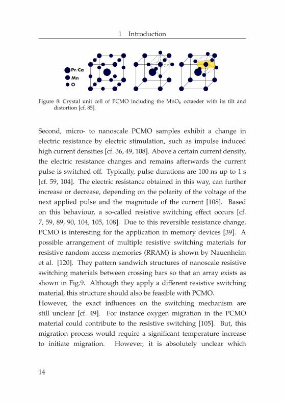
Figure 8: Crystal unit cell of PCMO including the MnO6 octaeder with its tilt anddistortion [cf. 85].
Second, micro- to nanoscale PCMO samples exhibit a change inelectric resistance by electric stimulation, such as impulse inducedhigh current densities [cf. 36, 49, 108]. Above a certain current density,the electric resistance changes and remains afterwards the currentpulse is switched off. Typically, pulse durations are 100 ns up to 1 s[cf. 59, 104]. The electric resistance obtained in this way, can furtherincrease or decrease, depending on the polarity of the voltage of thenext applied pulse and the magnitude of the current [108]. Basedon this behaviour, a so-called resistive switching effect occurs [cf.7, 59, 89, 90, 104, 105, 108]. Due to this reversible resistance change,PCMO is interesting for the application in memory devices [39]. Apossible arrangement of multiple resistive switching materials forresistive random access memories (RRAM) is shown by Nauenheimet al. [120]. They pattern sandwich structures of nanoscale resistiveswitching materials between crossing bars so that an array exists asshown in Fig.9. Although they apply a different resistive switchingmaterial, this structure should also be feasible with PCMO.However, the exact influences on the switching mechanism arestill unclear [cf. 49]. For instance oxygen migration in the PCMOmaterial could contribute to the resistive switching [105]. But, thismigration process would require a significant temperature increaseto initiate migration. However, it is absolutely unclear which
14

1 Introduction
Figure 9: Example for an arrangement of multiple resistive switching materials forresistive random access memories [cf. 120]. The grey bars are the top andbottom contacts for the electric current and the blue blocks represent the resistiveswitching material.
temperatures occur for such high current densities and whether theoccurring temperatures have significant influence on the temperaturedependent resistivity or not. Thus here, Joule heating could contributesignificantly to a thermally assisted switching [cf. 105]. Since it isexceedingly difficult to measure the temperature inside a small scalePCMO material experimentally, the influence of Joule heating on theelectric resistance is studied in this work numerically. In contrastto thin film investigations for thermoelectrics, micro- to nanoscalecylindrical PCMO samples (pillars) are investigated.
15

1 Introduction
1.2 Heat conduction in solids
In general, propagation of heat takes place by three different types ofheat transfer, as shown in Fig.10.
Figure 10: Different types of heat transfer: (a) heat conduction, (b) convection and (c)radiation.
Convection describes heat transfer between two media which are atdifferent temperatures. Here, at least one medium is a flowing fluid.Radiation is heat transfer by electromagnetic waves. In comparisonto convection, radiation does not need an additional medium to beinvolved [21, p. 4]. Thus, radiation can also take place in vacuum.Conduction describes heat transfer through electron and phononmovements and interactions within a body itself [cf. 145, 151].Conduction takes place when a temperature gradient exists in amaterial between two different points along an axis as shown in Fig.11.
Figure 11: Change of temperature.
According to Carslaw and Jaeger [35, p. 7], the flow of heat, per unittime and area, in the direction of x, is defined as heat flux
qx = −κ∂T∂x, (1.5)
16
1 Introduction
where κ is the thermal conductivity of the material and T thetemperature. For an isotropic solid, the fluxes in three dimensionsare defined as
qx = −κ∂T∂x, qy = −κ
∂T∂y
, qz = −κ∂T∂z. (1.6)
Using the gradient operator ∇ and combining the spatial fluxes to thevector identity ~q, Fourier’s law of heat conduction writes as
~q = −κ∇T . (1.7)
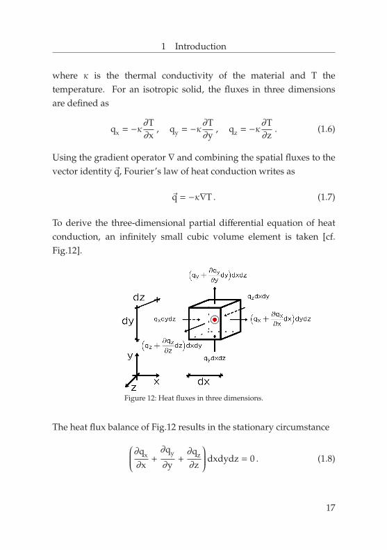
To derive the three-dimensional partial differential equation of heatconduction, an infinitely small cubic volume element is taken [cf.Fig.12].
Figure 12: Heat fluxes in three dimensions.
The heat flux balance of Fig.12 results in the stationary circumstance∂qx
∂x+∂qy
∂y+∂qz
∂z
dxdydz = 0 . (1.8)
17

1 Introduction
Time dependent temperature changes are taken into account by themass density ρ and the specific heat capacity cp through the termρcp
∂T∂t dxdydz [35, p. 9]. Thus, Eq. 1.8 becomes∂qx
∂x+∂qy
∂y+∂qz
∂z
+ ρcp∂T∂t
= 0 . (1.9)
If heat is generated in the volume, a source term p(x,y,z,t) has to beadded to the right hand side [35, p. 10] so that Eq. 1.9 develops to∂qx
∂x+∂qy
∂y+∂qz
∂z
+ ρcp∂T∂t
= p(x,y,z,t) . (1.10)
Substitution of the heat flux terms by the identities defined in Eq.1.6,the partial differential equation of heat conduction for isotropic solidsbecomes
−
(∂∂xκ∂T∂x
+∂∂yκ∂T∂y
+∂∂zκ∂T∂z
)+ ρcp
∂T∂t
= p(x,y,z,t) . (1.11)
If κ is constant, rearranging of Eq.1.11 gives
∂2T∂x2 +
∂2T∂y2 +
∂2T∂z2 −
1D∂T∂t
+p(x,y,z,t)
κ= 0 (1.12)
and points out the thermal diffusivity
D =κρcp
. (1.13)
18
1 Introduction
In case the temperature does not vary with time, Eq.1.11 simplifies tothe steady state formulation
−
(∂∂xκ∂T∂x
+∂∂yκ∂T∂y
+∂∂zκ∂T∂z
)= p(x,y,z) (1.14)
in which time-dependent parts do not exist. The previously discussedequations are valid for isotropic thermal conductions. However,naturally or artificially created materials can exhibit an anisotropy ofthermal conductivity in different spatial directions. The correspondingheat conduction equations are discussed in Sec.3.1.1. Furthermore, ithas to be mentioned that in general the thermal conductivity of onematerial is not constant but varies with temperature [cf. 35]. However,we neglect this effect in this work.
19

2 The 3ω-method
2.1 Concept, measurement principle and geometryconfigurations
ConceptThe 3ω-method is an alternating current (ac) technique to measure thethermal conductivity of micro- to nanoscale samples. This methodfinds its origin in the early 20th century. According to literature [133],Corbino [44] discovered a third harmonic component in the voltagesignal. Since then, various authors have exploited alternating currenttechniques to determine thermal properties of samples.10 For example,Birge et al. [16, 17] used 3ω-detection to measure the specific heatof super cooled liquids, such as glycerol and propylene glycol, nearthe glass transition phase in the 1980s. Approximately one decadelater, Cahill [28, 34] derived the analytic solution of the temperatureamplitude for a heater substrate system where the heater has a finitewidth. Contemporary literature dealing with the 3ω-method refersmostly to Cahill’s prominent work.
Measurement principleThe classical 3ω-method [28] uses a thin electrically conductingmetal strip deposited on the sample surface to measure the thermalconductivity. The metal strip functions as both the heater and thethermometer. An alternating current
I = I0 cos(ωt) (2.1)
10Dames et al. [47] compare different harmonic detections (1ω, 2ω, 3ω signals).
21

2 The 3ω-method
is applied onto the heater. Here, I0 is the peak current, ω is the angularfrequency and t is the time. A classical heater substrate structure isshown in Fig.13. The current is applied at the outer pads of the heater.
substr
ate
heate
r
I
Figure 13: Application of the alternating current at the outer pads.
Passing an alternating electric current through a metal strip with anelectric resistance R releases power P as heat, known as Joule heating.The released power writes as
P = R · I2 = R · I20 · cos2(ωt)
= R · I20 ·
12· (1 + cos(2ωt)) . (2.2)
The released power is shown in Fig.14.
Figure 14: Time dependent released power.
Here, P0 = R · I20 · 1/2 is the applied power amplitude. The time-average
mean component of the dissipated power produces a constanttemperature gradient with respect to the ambient temperature (T0 +
Tco), while the alternating component releases diffusive thermal waveswhich propagate into the sample. Hence, the general temperature rise
22

2 The 3ω-method
of the heater and the surrounding material is composed of an averagepart Tav and alternating part ∆T due to a constant and an alternatingpower input, respectively. The general temperature behavior is shownin Fig.15.
Figure 15: General temperature behavior.
Considering a possible phase shift ς, the temperature rise writes to
T = Tav + ∆T cos(2ωt + ς) . (2.3)
Thus, a sufficient time must be given in the measurement until thesystem reaches a ‘swung-in state’. The general temperature profileand the phase shift in the heater depend on the thermal conductivityand thermal mass of the sample material. Due to its temperaturedependence, the resistance of the metal strip R oscillates additionallyto an average resistance Rav at the modulated frequency 2ω with ∆Rso that
R = Rav + ∆R cos(2ωt + ς) . (2.4)
The inner pads of the metal strip are used to measure a voltage acrossthe heater [Fig.16].Substitution of Eq.2.1 and Eq.2.4 into Ohm’s law leads to a voltagesignal U,
U = I ·R = I0Rav cos(ωt) +I0∆R
2(cos(3ωt + ς) + cos(ωt + ς)) , (2.5)
23

2 The 3ω-method
substr
ate
heate
r
V
Figure 16: Measurement of the modulated voltage at the inner pads.
containing information at ω and 3ω.11 Relating the voltage signalto the desired thermal conductivity of the sample, a connection overthe temperature amplitude is required. In case of the 3ω-method, itis assumed that the resistance oscillation is linearly connected to thetemperature amplitude. This circumstance is shown in Fig.17
Figure 17: Temperature dependent resistance behavior.
and writes to
∆R =dRdT·∆T . (2.6)
Here, dT/dR is the specific temperature to resistance behavior ofthe heater. Rearranging Eq.2.6 and including the third harmoniccomponent of the voltage U3ω = I0∆R/2 and the peak voltageamplitude U1ω = I0Rav of the voltage at frequency ω , the temperature
11Find detailed and further information in App.A.1.
24

2 The 3ω-method
amplitude of the heater is given as [29]
∆T =dTdR·∆R = 2
dTdR·
U3ω
I0= 2
dTdR
Rav
U1ωU3ω . (2.7)
This relation connects the voltage measured in experiments to theanalytically described temperature amplitude. This connection isnecessary to identify the sample’s thermal conductivity.
Geometry configurationsThe third-harmonic detection is used in a wide range of applicationstoday. Although the working principle is consistent for eachapproach, different geometry configurations have different analyticaldescriptions for the temperature amplitude ∆T. One-dimensional likestructures, which are mainly free from mechanical supports, suchas standing nanopillars [148] or suspended nanowires/microwires[14, 110, 165] are studied or used to determine the thermal propertiesof surrounding matter such as gas [169] or fluids [87]. Moreover,different groups investigated heater substrate platform structures[cf. Sec.2.3] to determine the thermal conductivity of electricallynon-conducting [38, 117] and electrically conducting liquids [40]. Inthis work, heater substrate platform structures are further investigatedfor their potential to study bulk-like materials, patterned multilayerstructures, and thin films. Also, membrane structures are nowadaysused to determine the thermal conductivity of thin films. The groupof F. Volklein [159] has been applying membrane structures, made byMicro Electro Mechanical Systems (MEMS-structures), since the 1990s.Various groups are still investigating thermal properties with MEMSwhere other geometry structures are inappropriate to determine thethermal conductivity of the sample [cf. 58, 79, 82, 146].
25

2 The 3ω-method
Especially the in-plane thermal conductivity is emphasized bymembrane MEMS geometries. However, utilizing MEMS, requireseither restrictive assumptions, or a three-dimensional analysis for theheat flow. These assumptions concern radiation, heat flow along theheater into the contact pads, and the heat spread in the membrane itself[cf. 77]. To overcome the restrictive assumptions, three-dimensionalFinite Element simulations are performed in this work to take intoaccount several aspects of the heat flow. Furthermore, specialgeometry configurations of the heater structure are presented todetermine the cross- and in-plane thermal conductivity.
2.2 Top down geometry
2.2.1 Heat source on bulk materials
The origin for the theoretical analysis of the 3ω-method can be foundin the fundamental textbook of Carslaw and Jaeger [35]. They solvedthe partial differential equation of heat conduction [cf. Eq.1.11] in thefield Ω with a point source boundary condition Γ on a semi-infinite halfspace in two-dimensions [cf. Fig.18(a)]. In the case of the 3ω-method,the applied heat is given as power per length (P0/L) generated at thefrequency 2ω = 2 · 2 ·π · fc. Here, P0 is the amplitude of the appliedpower and considered to be constant. With the assumption that theheater length goes to infinity Lh(z)→ ∞, the substrate is semi-infiniteds → ∞, and the heat input is a point source, the temperatureoscillation at a distance r from the line source of heat reads as [35,p. 193]
∆T(r) =P0
LπκKB
0 (qr) . (2.8)
26

2 The 3ω-method
(a) (b)
(c)
Figure 18: Heat source on bulk materials: (a) Considered system for Carslaw and Jaeger[35]; (b) system for Cahill [28]; (c) system for Borca-Tasciuc et al. [22].
Here, i is the complex number, r =(x2 + y2
) 12 is the distance from the
line, κ the thermal conductivity of the semi-infinite material, KB0 the
modified Bessel function of second kind and zero order, and 1/q is thethermal penetration depth, defined as
1q
=( D
i2ω
) 12
. (2.9)
The thermal penetration depth describes the characteristic decay of thetemperature amplitude in the material, and thus how deep significanttemperature effects propagate into a medium during one cycle ofheating [cf. 13, p. 314]. Hence, the ratio between the temperatureamplitude at the surface and the temperature amplitude below thisdepth tends to zero. Consequently, possible changes of materialproperties below this depth (e.g. different layers of material) have
27

2 The 3ω-method
no retroactive influence on the temperature amplitude at the surface.Since the 3ω-method uses a thin metal strip, the heat source has a finitewidth [cf. Fig.18(b)]. To obtain the temperature amplitude over theheater width, it is convenient [28] to use the Fourier cosine transformof the temperature oscillation Eq.2.8 and the heater width itself. Themeasurement of the temperature takes place in the heater itself, thusat the surface of the sample. Therefore, y is set to zero so that only thex-coordinate remains in Eq.2.8 [28].The Fourier cosine transform is defined as [11, p. 3]
F (k) =
√2π
∫∞
0f(x) · cos(kx)dx . (2.10)
Based on this definition, the Fourier cosine transform of Eq.2.8 is givenas [11, p. 49]
Fp =
√2π·
P0
Lπκ·
14·
1√(k2 + q2)
· 2π =
√2π·
P0
L2κ·
1√(k2 + q2)
.
(2.11)
Assuming heat enters the substrate evenly over the heater width, theheater width can be regarded as a rectangular function
h =
1b , 0 ≤ x ≤ b
0, x > b(2.12)
with respect to the symmetry at x = 0, shown in Fig.19 [cf. 27, 111].Here, b is the half heater width.
28

2 The 3ω-method
Figure 19: Rectangular function for the heater width.
Using Eq.2.10, the Fourier cosine transform of this rectangular functionwrites to
Fb(k) =
√2π
∫ b
0
1b· cos(kx)dx =
√2π·
sin(kb)kb
. (2.13)
In Fourier space, convolution [26, p. 24] of Eq.2.11 and Eq.2.13 resultsin
Fc(k) = Fp(k) · Fb(k) =2π·
P0
L2κ·
sin(kb)
kb ·√
(k2 + q2). (2.14)
The inverse Fourier cosine transform of the convoluted temperatureoscillation writes to
∆Th(x) =
∫∞
0Fc(k) · cos(kx)dk
=P0
Lπκ·
∫∞
0
sin(kb) · cos(kx)
kb ·√
(k2 + q2)dk . (2.15)
The latter equation describes the local temperature amplitude fromthe center of the heater towards its side. However, since the measuredtemperature amplitude is a mean value over the heater width, it isappropriate to average the temperature amplitude through integration
29

2 The 3ω-method
0.00
0.20
0.40
0.60
0.80
1.00
100 101 102 103 104 105 106
∆T
[K]
Frequency fc [Hz]
Solution ofSolution ofSolution of
(a)Eq.2.17Eq.2.18Eq.2.21
0.00
0.04
0.08
0.12
0.16
0.20
100 101 102 103 104 105 106
∆T
[K]
Frequency fc [Hz]
Solution ofSolution ofSolution of
(b)Eq.2.17Eq.2.18Eq.2.21
Figure 20: Cahill’s solution of Eq.2.17, Eq.2.18 and Eq.2.21 for a heat source on bulk-likematerials with P0/L = 5 W/m and 2b = 10 µm for the substrate materials (a) STOand (b) MgO.
so that
12b
∫ b
−b∆Th(x)dx =
P0
Lπκ·
12b·
2k
∫∞
0
sin(kb) · sin(kb)
kb ·√
(k2 + q2)dk . (2.16)
This is the proposed solution of Cahill [28] for the temperatureamplitude measured by the heater
∆TCh =
P0
Lπκs
∫∞
0
sin2(kb)
(kb)2√
k2 + q2dk . (2.17)
Here, κs is the thermal conductivity of the substrate. The subscriptsh and s indicate heater and substrate respectively. The height andthermal properties of the heater are neglected and no thermal resistancebetween the heater and the substrate is taken into account.Moreover, Cahill [28] proposed an approximate solution for the casethat the thermal penetration depth is large in comparison to the halfheater width (q−1
b → bq 1).
30

2 The 3ω-method
First, he sets the limits of the integral from 0 to 1/b so that
∆TCh =
P0
Lπκs
∫ 1/b
0
sin2(kb)
(kb)2√
k2 + q2dk . (2.18)
Second, he assumes that
sin2(kb)(kb)2 = 1 . (2.19)
Underlying these assumptions, Cahill simplifies the general solutionof Eq.2.17 to
∆TCh =
P0
Lπκs
∫ 1/b
0
1√k2 + q2
dk (2.20)
=P0
Lπκs
[−
12
ln(ω) −12
ln(
ib2
D
)+ const
]. (2.21)
This linearized description contains a frequency dependentreal part Re(∆TC
h ) = [−1/2 · ln(ω) + const] and an imaginary partIm(∆TC
h ) = [−1/2 · ln(ib2/D
)].12 The frequency dependent temperature
amplitude Re(∆TCh ) is shown in Fig.20 for the solution of Eq.2.17,
Eq.2.18 and Eq.2.21.13 First, the low frequency regime is considered.While the solutions exhibit different axis intercepts, the slope of the∆T -lines are the same so that these lines are parallel. However,Eq.2.21 shows how the thermal conductivity of an isotropic substratecan be determined from the slope of the real part Re(∆TC
h ) of thecomplex temperature amplitude versus the logarithm of the frequency.12Find App.A.3 for detailed information on the derivation and the constant.13In this work, we only plot the real part of the temperature amplitude Re(∆T) and
reduce the labelling of the axis to ∆T.
31

2 The 3ω-method
0.0000
0.0002
0.0004
0.0006
0.0008
0.0010
100 101 102 103 104 105
Thermalpen
etrationdep
th[m
]
Frequency fc [Hz]
MgOSTO
(a)
0
1
2
3
4
5
6
100 101 102 103 104 105
bq[-]
Frequency fc [Hz]
MgOSTO
(b)
Figure 21: (a) Thermal penetration depth q−1 and (b) restriction bq 1 for two differentmaterials.
Given by the linear behavior in the low frequency regime, such as inFig.:20(a) and Fig.:20(b), the thermal conductivity of the substrate canbe extracted by
κs = −P0
Lπ2·
1d
d ln(ω) Re(∆TCh )
= −P0
Lπ2d ln(ω)
d Re(∆TCh )
(2.22)
from the slope. Hence, the different axis intercepts do not matter ifthe thermal conductivity is determined in this way. From a physicalperspective, the linearized solution of Eq.2.21 is only valid forfrequencies where the temperature amplitudes are greater than zeroso that ∆T > 0. Amplitudes equal or smaller than zero can not occur.Second, the high frequency regime is considered. Here, the solutionsexhibit a different curve progression. This difference occurs, becauseat higher frequencies, the thermal penetration depth is on the order ofthe half heater width [cf. Fig.21(a)]. In this case bq 1 is not fulfilled[cf. Fig.21(b)].
32

2 The 3ω-method
Despite the small thickness of the metal strip, the heat source stillhas a finite height. Since a heat source with a finite height andwidth represents a cross-section of a material, it is of interest to takeinto account its material properties for a more realistic description.Borca-Tasciuc et al. [22] considered this circumstance so that thetemperature amplitude over the heater width at the surface of thesample writes to
∆TBH =
∆TBh
1 + (ρHcpH)ai2ω∆TB
h2b LP0
, (2.23)
where
∆TBh =
-P0
Lπκcrs1
∫∞
0
1χ
sin2(kb)
k2b2 dk . (2.24)
Here, a is the height of the heater, ρHcpHis the thermal mass of
the heater and κcrs1 is the cross-plane thermal conductivity of thematerial below the heat source. ∆TB
h is Borca-Tasciuc’s solution ofthe temperature amplitude without material properties of the heater.The complex term χ contains information about the materials belowthe metal strip, like the incorporated finite substrate thickness [cf.Fig.18(c)]. For a semi-infinite isotropic substrate this solution is equalto Cahill’s solution of Eq.2.17. However, this term is discussed indetail in Sec.2.2.2. It has to be noted, that the thermal conductivityof the metal strip is still neglected. Also a thermal contact resistancebetween the heater and the investigated material can be regarded inEq.2.23, but this influence factor is not considered in this work.A comparison of Cahill’s and Borca-Tasciuc’s solutions in Fig.22indicates the differences in the inset for various frequency regimes.
33

2 The 3ω-method
0.00
0.20
0.40
0.60
0.80
1.00
100 101 102 103 104 105 106
∆T
[K]
Frequency fc [Hz]
0.000
0.005
0.010
100 105
diff
.
Solution ofSolution ofSolution of
Eq.2.17Eq.2.23Eq.2.23, ds
Figure 22: Comparison of Cahill’s solution of Eq.2.17 and Borca-Tasciuc’s solutions ofEq.2.23 with an infinite and finite substrate. ds indicates the considered substratethickness of 1 mm for an STO substrate. The inset contains the detailed differencebetween the solutions of Eq.2.23 with respect to Eq.2.17. The height of theplatinum heater is a = 100 nm.
Eq.2.23 can be solved with respect to an infinite and finite substratethickness. The solution of Eq.2.23 for a substrate with finite thicknessand adiabatic boundary condition differs slightly in the low frequencyregime from the solution for an infinite substrate [cf. Fig.22]. Here,the boundary of the substrate interacts with the thermal penetrationdepth. On the contrary, the thermal penetration depth is small forhigh frequencies. Thus, the solution for an infinite and finite substratethickness is coincident in the high frequency regime in the inset ofFig.22. However, in the high frequency regime, the influence of thematerial properties of the heater become pronounced. This is dueto the small thermal penetration depth, being on the order of theheaters width. Traditionally, 3ω-measurements are performed in afrequency regime between 1 Hz and 10 kHz [cf. 28], and the thermalconductivity of the heater and substrate are on the same order ofmagnitude. Usually, the thermal properties of the heater can beneglected within these boundaries [cf. 152]. However, the limitationof this assumption is discussed more in detail in Sec.2.2.2.
34
2 The 3ω-method
2.2.2 Heat source on layer-substrate materials
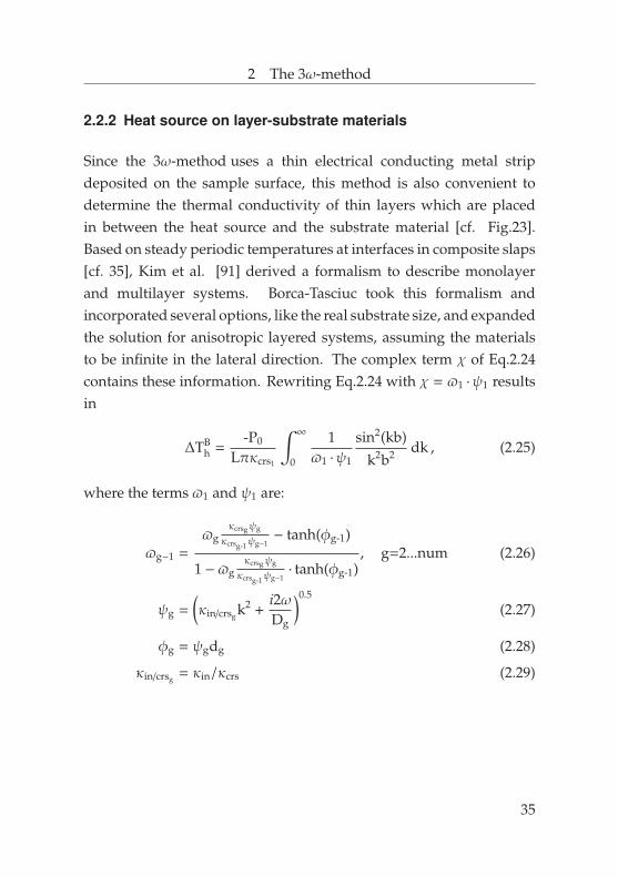
Since the 3ω-method uses a thin electrical conducting metal stripdeposited on the sample surface, this method is also convenient todetermine the thermal conductivity of thin layers which are placedin between the heat source and the substrate material [cf. Fig.23].Based on steady periodic temperatures at interfaces in composite slaps[cf. 35], Kim et al. [91] derived a formalism to describe monolayerand multilayer systems. Borca-Tasciuc took this formalism andincorporated several options, like the real substrate size, and expandedthe solution for anisotropic layered systems, assuming the materialsto be infinite in the lateral direction. The complex term χ of Eq.2.24contains these information. Rewriting Eq.2.24 with χ = $1 ·ψ1 resultsin
∆TBh =
-P0
Lπκcrs1
∫∞
0
1$1 ·ψ1
sin2(kb)
k2b2 dk , (2.25)
where the terms $1 and ψ1 are:
$g−1 =$g
κcrsgψg
κcrsg-1ψg−1− tanh(φg-1)
1 − $gκcrsgψg
κcrsg-1ψg−1· tanh(φg-1)
, g=2...num (2.26)
ψg =(κin/crsg k2 +
i2ωDg
)0.5
(2.27)
φg = ψgdg (2.28)
κin/crsg = κin/κcrs (2.29)
35

2 The 3ω-method
dlayΩ
Γ
2b
substrate
(a)
dlay
Ω
Γ
2b
substrate
(b)
Figure 23: Heat source on layer-substrate materials: Schematic heat spread for (a) broadheaters on thin layers and for (b) narrow heaters on thick layers.
Here, num is the total number of layers (including the substrate) forthe corresponding subscript g. The subscript g belongs to the gth layer,starting from top, down to the substrate. The subscript crs indicatesthe cross-plane value of the corresponding quantity. The materialproperties of each layer are given by the thickness dg and the respectivethermal diffusivity Dg. The effect of anisotropic thermal conductionis taken into account by κin/crs, the ratio of in-plane to cross-planethermal conductivity. For a semi-infinite substrate $num = −1 whilefor a finite thickness, $num = −tanh(ψnumdnum) for an adiabatic and$num = −1/tanh(ψnumdnum) for an isothermal boundary condition[22].14 However, the solution of Borca-Tasciuc is rather inconvenientto determine the thermal conductivity of an investigated material,since this convoluted solution is very processor-intensive, especiallyfor anisotropic multilayer structures. But treating the investigatedstructures with some assumptions for the heat flow, Lee and Cahill [99]proposed an elegant solution to determine the thermal conductivitiesof thin poorly-conductive dielectric layers.15
14The solutions of Borca-Tasciuc are useful to understand complete system behaviors,but depending on the numbers of layers and other conditions, computation costs canbe high.
15Also previously, numerous studies were published by Cahill’s group, dealing with thedetermination of thin layer thermal conductivities, such as [32],[30] and [100].
36

2 The 3ω-method
Figure 24: General system behaviour for the offset model.
The so-called offset model [99] regards a poorly-conductive layer asa one-dimensional thermal resistor, so that the cross-plane thermalconductivity can be determined. This model assumes the half heaterwidth to be much greater than the thickness of the layer and the thermalconductivity of the substrate to be much greater than the thermalconductivity of the layer:
b dlay
κs κlay
offset model (2.30)
Given these circumstances, a parallel shift along the temperatureamplitude axis arises in the low frequency regime onto the solution ofa heater substrate system [cf. Fig.24]. Here, the low frequency regimecorresponds to the restriction bq 1, given in Sec.2.2.1. The overallmeasured temperature amplitude in the heater ∆TC
hls is now composedof the temperature amplitude by the substrate ∆TC
h of Eq.2.17 and anadditional temperature amplitude of the thin layer ∆TC
lay. This seriesconnection writes to
∆TChls = ∆TC
lay + ∆TCh . (2.31)
37
2 The 3ω-method
With this temperature amplitude offset, the thermal conductivity ofthe investigated layer can be determined by
∆TClay =
P0
Lκlay
dlay
2b. (2.32)
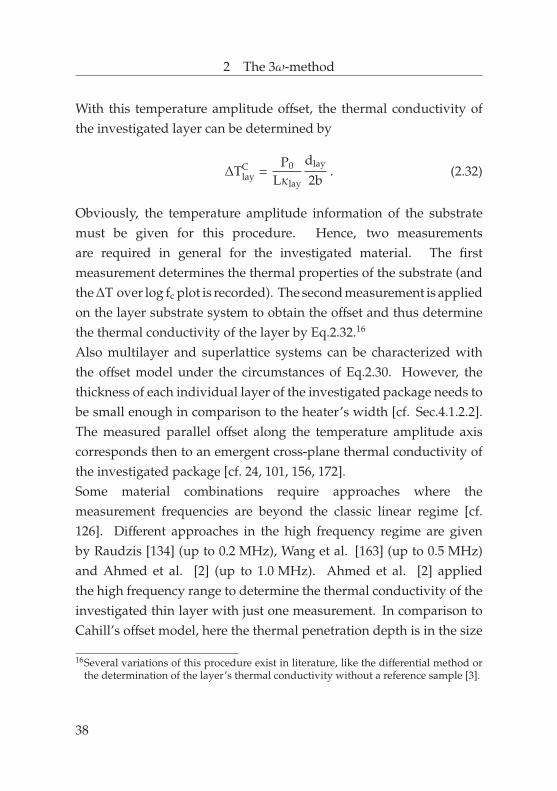
Obviously, the temperature amplitude information of the substratemust be given for this procedure. Hence, two measurementsare required in general for the investigated material. The firstmeasurement determines the thermal properties of the substrate (andthe ∆T over log fc plot is recorded). The second measurement is appliedon the layer substrate system to obtain the offset and thus determinethe thermal conductivity of the layer by Eq.2.32.16
Also multilayer and superlattice systems can be characterized withthe offset model under the circumstances of Eq.2.30. However, thethickness of each individual layer of the investigated package needs tobe small enough in comparison to the heater’s width [cf. Sec.4.1.2.2].The measured parallel offset along the temperature amplitude axiscorresponds then to an emergent cross-plane thermal conductivity ofthe investigated package [cf. 24, 101, 156, 172].Some material combinations require approaches where themeasurement frequencies are beyond the classic linear regime [cf.126]. Different approaches in the high frequency regime are givenby Raudzis [134] (up to 0.2 MHz), Wang et al. [163] (up to 0.5 MHz)and Ahmed et al. [2] (up to 1.0 MHz). Ahmed et al. [2] appliedthe high frequency range to determine the thermal conductivity of theinvestigated thin layer with just one measurement. In comparison toCahill’s offset model, here the thermal penetration depth is in the size
16Several variations of this procedure exist in literature, like the differential method orthe determination of the layer’s thermal conductivity without a reference sample [3].
38

2 The 3ω-method
of the layer’s thickness. A fit is subsequently used to determine thethermal conductivity of the thin layer by the characteristic transitionzone in the ∆T plot [cf. Sec.4.1.2]. This approach demonstratesthe upper limit of feasible frequencies, but would also require theconsideration of the thermal properties of the heater [cf. Sec.4.1.2].Although the offset model is applied on geometrical systems, wherethe half heater width is much greater than the thickness of the layer, theslight in-plane heat spread affects the temperature amplitude even forpoorly-conductive layers. This in-plane heat spread needs to be takeninto account in order to determine accurate thermal conductivities [cf.Fig.23]. Cahill and Lee [33] introduced a correction value in terms ofan effective heater width, so that
2beff = 2b + 0.88 ·dlay . (2.33)
This corrected offset model is compared in Sec.4.1.2 with the solutionof Borca-Tasciuc and the Finite Element simulations of this work.In general, a reduction of the heater’s width 2b towards the dimensionof the layer’s thickness dlay increases the influence of the in-planeheat spread. Moreover, the influence on the temperature amplitudealso increases for moderately- and highly-conductive layer materials.Thus, the in-plane thermal conductivity can be determined in general.Therefore, two measurements are required to distinguish between thecross- and in-plane thermal conductivity. The cross-plane thermalconductivity measurement applies a broad heater while the in-planemeasurement applies a narrow heater [cf. Fig.:23].This approach is used by Borca-Tasciuc et al. [22] to determine thethermal conductivity of 60 µm thick nanochanneled aluminum.
39

2 The 3ω-method
Also, multilayer and superlattice structures with a total thicknessof 1 − 2 µm are investigated by several groups [cf. 22, 23, 152]. Inthese references, either a tremendous thickness, or moderately- andhighly-conductive layer materials are investigated. But as mentionedin Sec.1, poorly-conductive layer materials are a prerequisite for futurethermoelectrics.However, in this work, the individual thickness of the investigatedmaterials is on the order of 0.1 − 0.5 µm and hence up to ten timessmaller. Here, the latter approach is no longer suitable, sincevariations in ∆T are smaller than the measurement accuracies forclassic measuring configurations. Given these circumstances, thereis still a necessity to develop new measuring configurations forthe cross- and in-plane thermal conductivity determination of thinpoorly-conductive nanoscale materials.
2.3 Bottom electrode geometry
2.3.1 Heat source between bulk-like materials
In contrast to top down geometries, inverse 3ω-method systems havethe heater in between two materials, a so-called bottom electrodegeometry. Moon et al. [117] used an inverse application of the3ω-method to measure the dynamic specific heat and the thermalconductivity of liquids. Based on the one-dimensional heat diffusion,the solution of the temperature amplitude with material on theopposite side of a planar heater is derived under the assumption ofsemi-infinite materials [cf. Fig.25(a)].
40

2 The 3ω-method
(a) (b)
(c)
Figure 25: Heat source between bulk-like materials: (a) Considered system for Moon etal. [117]; (b) system for Chen et al. [38]; (c) system for Choi et al. [40].
In this case, the extracted thermal conductivity is a sum of the thermalconductivities of the two materials
κs + κm = −P0
Lπ2d ln(ω)
d Re(∆TCh ), (2.34)
where, the subscript m indicates the material to be investigated [117].However, since a real heater has a finite height, this solution is notexact because the ambient material on top encloses the heater [cf.Fig.25(b)]. A so-called boundary mismatch [38] exists due to a heatflow across the side walls of the heater into the liquid. Chen et al. [38],designed a 3ω-method technique to measure the thermal conductivityof liquids and solids, introducing an empirical correction value Θ dueto the boundary mismatch to reduce the error for the extracted thermalconductivity.
41

2 The 3ω-method
Thus, Eq.2.34 rewrites to
κs + Θ ·κm = −P0
Lπ2d ln(ω)
d Re(∆TCh ). (2.35)
Choi et al. [40] proposed a bottom electrode application for the3ω-method to measure electrically conducting liquids. For this, a thindielectric layer is deposited on top of the heater to prevent electricalleakage [cf. Fig.25(c)]. Here, the measurements are carried out at lowfrequencies to ensure the thermal wave penetrates into the liquid.17
Both, the contour shape of the covering layer and its thermal propertiesare neglected.
2.3.2 Heater substrate platform
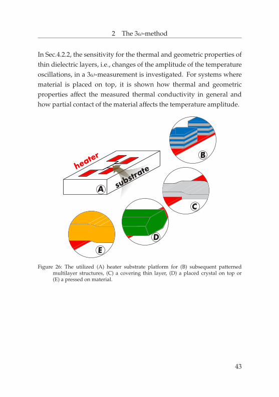
In contrast to top down approaches, where the heat source is alwaysabove the investigated material, thin layers on top of the heat sourceare of special interest in this work. In this thesis, the potential fora new heater substrate platform is investigated for nanostructuredmaterials.18 By always using the same heater substrate platformas sample holder, an optimum reproducibility of the investigatedmaterials could be achieved. The platform, shown in Fig.26(A), couldbe utilized to study subsequently patterned multilayer structures (B),covering thin layers (C) or materials placed on top. In this work,placing implies any method to establish thermal contact to the heatersuch as gluing, pressing, or bonding for materials which cannot bedeposited. Examples are brittle crystals (D) or bulk-like materials (E).
17Similar applications are done for nano- and subnanoliter fluids [124, 127].18Utilizing a heater substrate platform for nanostructured materials was the idea of the
joint project and especially the group around Jooss.
42
2 The 3ω-method
In Sec.4.2.2, the sensitivity for the thermal and geometric properties ofthin dielectric layers, i.e., changes of the amplitude of the temperatureoscillations, in a 3ω-measurement is investigated. For systems wherematerial is placed on top, it is shown how thermal and geometricproperties affect the measured thermal conductivity in general andhow partial contact of the material affects the temperature amplitude.
substra
te
A
B
C
D
E
heate
r
Figure 26: The utilized (A) heater substrate platform for (B) subsequent patternedmultilayer structures, (C) a covering thin layer, (D) a placed crystal on top or(E) a pressed on material.
43


3 Finite Element Model
Finite Element modeling has two decisive advantages for thethermal conductivity determination of nanoscale materials. First,multiphysical coupling of several macroscopic influence factors allowsstudying derivations from analytical descriptions and hence lead tohigh precision analysis. Accordingly, the overall understanding of the3ω-method can be furthered. Second, new measuring configurationscan be developed where no analytic solutions are available and thusopen new possibilities for nanostructured materials.In general, the partial differential equation of heat conduction has tobe solved. Since the 3ω-measurement takes place in a steady stateoscillation level, where the temperature amplitude ∆T oscillates upona constant temperature gradient [cf. Sec.2.1], one could just performa harmonic analysis. However, this work applies a combination ofsteady-state and a time-dependent analysis. By this combination, alsothe absolute measuring temperatures can be evaluated besides thedetermination of the temperature amplitudes.In this work, COMSOL MultiphysicsR© is used for Finite Elementanalysis. The interior mathematics interface for partial differentialequations is applied to implement the required macroscopicconditions. Therefore, the governing equations are deduced in thefollowing sections to the form of their partial differential equationexistence.19
19An introduction for the governing equations of the temperature field is also given byWang et al. [161].
45

3 Finite Element Model
3.1 Governing equations
3.1.1 Temperature field
We distinguish between three different general areas. The area of thesubstrate, the heater and the investigated material [Fig.27]. If possible,the system simplified through axis of symmetry.
dlay/m
2b
ds
dlay/ma
bsys
Γ
Γ
Γ
Γ
Ω
ΩΩH lay/m
lay/m
Ωs
4
3
2
1x
y
z
Figure 27: System definition of areas and boundaries.
46

3 Finite Element Model
The substrate is considered to be isotropic and without any sourceterms for heat dissipation, so that the partial differential equation canbe expressed as
Ωs :∂2Ts
∂x2 +∂2Ts
∂y2 +∂2Ts
∂z2 −1
Ds
∂Ts
∂t= 0 . (3.1)
Here Ds is the diffusivity of the substrate. Also the heater is assumedto be isotropic so that
ΩH :∂2TH
∂x2 +∂2TH
∂y2 +∂2TH
∂z2 −1
DH
∂TH
∂t+
pκH
= 0 . (3.2)
Here, κH is the thermal conductivity of the heater. We take into accounta linear temperature coefficient α so that the heat source term p ofEq.:3.2 reads as
p = %0 · (1 + α · (T − T0)) · j20 ·12· (1 + cos(2ωt)) . (3.3)
Here, T0 is the ambient temperature and j0 is the peak currentdensity. Since the 3ω-method applies a power per unit length W/1min z-direction, but is not specific about the heater’s properties, thecorresponding current density must be calculated. We calculate thepeak current with the specific electric resistivity %0 at room temperatureby
P0
L=%0
A· I2
0 → I0 =
√P0%0 ·L
A
, (3.4)
where L is the length of the heater and A is the cross-sectional area ofthe heater.
47
3 Finite Element Model
The peak current density of Eq.3.3 is now calculated by
j0 =I0
A. (3.5)
The thermal conductivity coefficients of a three-dimensionalanisotropic solid are components of a second-order tensor [cf. 35].In this work, we distinguish between pure in-plane and cross-planethermal conduction since we focus on thin layered materials. Hence,the governing equation of the anisotropic investigated material is
Ωlay/m : κmin
∂2Tm
∂x2 + κmcrs
∂2Tm
∂y2 + κmin
∂2Tm
∂z2 − ρmcpm
∂Tm
∂t= 0 .
(3.6)
Here κmin and κmcrs represent the in-plane and cross-plane thermalconductivities respectively. Tm is the temperature and ρmcpm
is thethermal mass of the investigated material. In case of two-dimensionalsimulations, the derivatives in z-direction do not exist so that ∂
∂z = 0.For all areas, the intended measuring temperature represents the initialcondition for the temperature
Ω : T(t = 0) = Tinit , (3.7)
where, Tinit is the initial temperature and T(t = 0) is the intendedmeasuring temperature at time zero.Since the investigation of various geometric structures in Sec.4 requiresdifferent boundary conditions (BC), these conditions are given in eachsection respectively.
48

3 Finite Element Model
However, we assume for every investigation ideal thermal contactbetween all materials [cf. 91] so that
Tk = Tk+1 . (3.8)
Thus, the interface boundary conditions for the heat flux write to
ΓInt : κk∂Tk
∂n= κk+1
∂Tk+1
∂n. (3.9)
Here, the subscript k and k+1 indicate two contacting materials.However, it has to be mentioned, that interface effects can influencethe heat transfer significantly under special circumstances [31].The occurring temperature amplitude is determined by
∆T = Tmeanmax − Tmeanmin . (3.10)
Here, Tmeanmax and Tmeanmin are the maximum and minimum meantemperature within one cycle of heating.20 The time dependent meantemperature in the heater depends on the spatial dimensions of theinvestigation. In the following we distinguish between three differentcases.First, for the validation of the Finite Element solution, a heat flux BCis used and thus the time dependent mean temperature is determinedover the heater width b by
Tmean(t) =1b·
∫ b
0T(t)dx . (3.11)
20In the following work, we distinguish between the term mean and average in themanner, that mean refers to a spatial coincident and average to a time dependentcoincident.
49

3 Finite Element Model
Second, the time dependent mean temperature for a heater with heighta and width b is determined by
Tmean(t) =1
a · b·
∫ a
0
∫ b
0T(t)dxdy . (3.12)
Third, in case of a three-dimensional investigation, the time dependentmean temperature is determined by
Tmean(t) =1
a · 2b ·L·
∫ L
0
∫ a
0
∫ 2b
0T(t)dxdydz . (3.13)
In contrast to a 3ω-measurement, the PCMO pillar studies exhibit arotation symmetry since the sample is basically a cylinder. The systemand the coordinate system definition is shown in Fig.28.
(a) (b)
Figure 28: PCMO pillar: 28(a) System and axis definition and 28(b) reduction to cylindercoordinates.
Consequently, the partial differential equations of each material can betransferred to cylindrical coordinates with respect to cosine and sinusfunctions. Here, we consider every material to be isotropic.
50

3 Finite Element Model
Hence, the respective partial differential equations for the substrate,layer and heating PCMO material become [cf. 35, 132]:
Ωs :
∂2Ts
∂r2 +1r∂Ts
∂r+
1r2
∂2Ts
∂θ2 +∂2Ts
∂z2 −1
Ds
∂Ts
∂t= 0 (3.14)
Ωlay/m :
∂2Tlay/m
∂r2 +1r∂Tlay/m
∂r+
1r2
∂2Tlay/m
∂θ2 +∂2Tlay/m
∂z2 −1
Dlay/m
∂Tlay/m
∂t= 0
(3.15)
ΩH :
∂2TH
∂r2 +1r∂TH
∂r+
1r2
∂2TH
∂θ2 +∂2TH
∂z2 −1
DH
∂TH
∂t+
pκH
= 0 (3.16)
In this work, these pillar configurations are studied up to severalhundred Kelvin. Here, a linear temperature coefficient is not sufficientto study the temperature development accurately. Therefore, thiswork applies a non-linear temperature dependent specific electricresistivity which was measured in experiments. The dissipated poweris discussed in Sec.4.4 together with the electric resistance behavior.Like for the 3ω-method simulations, we assume here also ideal thermalcontact between all materials. The boundary conditions for the outerboundaries are given in Sec.4.4. The mean temperature of the heatingPCMO material is determined by
Tmean(t) =1
πr2p ·dPCMO
·
∫ dPCMO
0
∫ rp
02πr ·T(t)drdz . (3.17)
Here, dPCMO is the thickness of the PCMO heating material. Theresulting temperature amplitude is again determined by Eq.3.10.
51
3 Finite Element Model
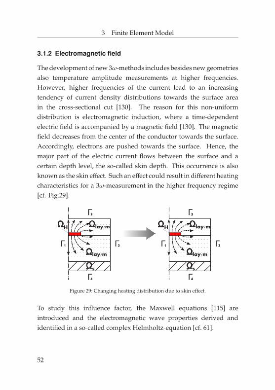
3.1.2 Electromagnetic field
The development of new 3ω-methods includes besides new geometriesalso temperature amplitude measurements at higher frequencies.However, higher frequencies of the current lead to an increasingtendency of current density distributions towards the surface areain the cross-sectional cut [130]. The reason for this non-uniformdistribution is electromagnetic induction, where a time-dependentelectric field is accompanied by a magnetic field [130]. The magneticfield decreases from the center of the conductor towards the surface.Accordingly, electrons are pushed towards the surface. Hence, themajor part of the electric current flows between the surface and acertain depth level, the so-called skin depth. This occurrence is alsoknown as the skin effect. Such an effect could result in different heatingcharacteristics for a 3ω-measurement in the higher frequency regime[cf. Fig.29].
Γ
Γ
Γ
Γ
Ω
ΩΩH lay/m
lay/m
Ωs
4
3
2
1Γ
Γ
Γ
Γ
Ω
ΩΩH lay/m
lay/m
Ωs
4
3
2
1
Figure 29: Changing heating distribution due to skin effect.
To study this influence factor, the Maxwell equations [115] areintroduced and the electromagnetic wave properties derived andidentified in a so-called complex Helmholtz-equation [cf. 61].
52
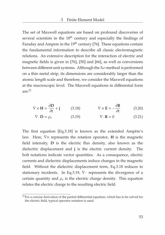
3 Finite Element Model
The set of Maxwell equations are based on profound discoveries ofseveral scientists in the 18th century and especially the findings ofFaraday and Ampere in the 19th century [76]. These equations containthe fundamental information to describe all classic electromagneticrelations. An extensive description for the interaction of electric andmagnetic fields is given in [76], [50] and [66], as well as conversionsbetween different unit systems. Although the 3ω-method is performedon a thin metal strip, its dimensions are considerably larger than theatomic length scale and therefore, we consider the Maxwell equationsat the macroscopic level. The Maxwell equations in differential formare:21
∇ ×H =∂D∂t
+ j (3.18)
∇ ·D = ρe (3.19)
∇ × E = −∂B∂t
(3.20)
∇ ·B = 0 (3.21)
The first equation [Eq.3.18] is known as the extended Ampere’slaw. Here, ∇× represents the rotation operator, H is the magneticfield intensity, D is the electric flux density, also known as thedielectric displacement and j is the electric current density. Thebolt notations indicate vector quantities. As a consequence, electriccurrents and dielectric displacements induce changes in the magneticfield. Without the dielectric displacement term, Eq.3.18 reduces tostationary incidents. In Eq.3.19, ∇ · represents the divergence of acertain quantity and ρe is the electric charge density. This equationrelates the electric charge to the resulting electric field.
21For a concise derivation of the partial differential equation, which has to be solved forthe electric field, typical operator notation is used.
53

3 Finite Element Model
Eq.3.20 is the Faraday’s law of induction. Here, E is the electric fieldintensity and B is the magnetic flux density. This equation statesthat a time dependent magnetic flux density changes the electric field.Eq.3.21 states that the magnetic flux density is solenoidal, so that nomagnetic monopoles exist.The current continuity equation can be obtained by taking thedivergence of the extended Ampere’s law [Eq.3.18] and subsitutingEq.3.19. Thus, the continuity equation writes to:
∇ ·
(∂D∂t
+ j)
= ∇ · (∇ ×H) ≡ 0 →∂ρe
∂t+ ∇ · j = 0 (3.22)
Since a 3ω-measurement takes place at a steady state oscillation level,it is quite convenient to transform the Maxwell equations, underassumptions of time harmonic fields and linear material relations,into their complex form. Assuming that no phase shift exists, thetime dependence cos(ωt) can be expressed with a complex exponentialfunction22 to
cos(ωt) =12
(eiωt + e−iωt) . (3.23)
It is common to replace the whole cosine just with eiωt [130, p. 368].While the first time derivative of the exponential function eiωt is iωeiωt,the time derivatives in the Maxwell equations are just represented bythe prefactor iω. Consequently, time does not appear explicitly. Thedetailed transformation behavior for this is shown in [130, p. 368].
22cos(z) = 12 (eiz + e−iz)
54

3 Finite Element Model
Hence, the Maxwell equations in complex form are:
∇ ×H = iωD + J (3.24)
∇ ·D = ℘e (3.25)
∇ × E = −iωB (3.26)
∇ ·B = 0 (3.27)
The blackboard bold typing in Eq.3.18-3.21 indicates the complexquantities. The corresponding current continuity equation writes to
−iω℘e + ∇ · J = 0 . (3.28)
To connect the Maxwell equations to matter, constitutive relations arenecessary. The general relations for linear material behaviour write to
D = εE , (3.29) B = µH , (3.30) J = σecE . (3.31)
Here, ε is the permittivity, µ is the permeability and σec is the electricalconductivity. For a linear and isotropic material, the permittivity ε andthe permeability µ are scalar and constant. Both consist of a vacuumconstant and a relative part due to the specific material. Thus, thepermittivity is ε = ε0εr and the permeability is µ = µ0µr [66, p. 180, p.275].In this work, an approach with the so-called magnetic vector potentialAj is used to determine the influence of the skin effect [cf. 5, 18–20, 103,130, 139]. This approach applies the magnetic vector potential as anauxiliary quantity to represent field variables.23 According to literature[19], the advantage of this potential is to reduce the overall degrees of
23The derivation and details of this quantity is given in [57, p. 14-1].
55

3 Finite Element Model
freedom and thus save computing costs. Already in the 1980 − 1990th,this approach was frequently encountered to solve electromagneticproblems [cf. 19, 103]. The magnetic vector potentialAj [66, p. 416] isintroduced to the magnetic flux density so that
B = ∇ ×Aj . (3.32)
With this definition of the magnetic flux density, Eq.3.26 rewrites to
E = −iωAj . (3.33)
The definition of the magnetic vector potential arises with a certainfreedom for the potential. Here, it is possible to add a gradient of ascalar function to the magnetic vector potential [76, p. 140], such as
Aj → A′
j = Aj + ∇ f , (3.34)
without changing the magnetic field density since
∇ × (∇ f ) = 0 . (3.35)
Furthermore, a transversal gauge transformation is given by
∇ ·Aj = 0 , (3.36)
which is the so-called Coulomb gauge transformation. The physicalstatement of Eq.3.36 is that the magnetic vector potential, and thus thefields, are perpendicular to the direction of propagation [50, p. 174].Now, the magnetic vector potential complies with the wave equationsand thus, the extended Ampere’s law and Faraday’s law can now be
56

3 Finite Element Model
rearranged into a form where the magnetic and electric field intensityare completely decoupled [cf. 76].24 However, both forms containinformation about the electromagnetic wave and thus the skin depth.25
We use a form of the extended Ampere’s law [Eq.3.24] which can berewritten to
(iωσec − ω2ε) ·Aj + ∇ × µ−1
∇ ×Aj = 0 , (3.37)
where just the magnetic vector potential is the degree of freedom.26
Essentially, Eq.3.37 can be rearranged and compared to a so-calledcomplex Helmholtz-equation27 for waves [cf. 61] in which the complexquantity k is identified by
−∇ · (µ−1∇Aj)+k2Aj = 0 (3.38)
k =√
iωσec − ω2ε . (3.39)
According to literature [130, p. 374], terms of higher order can beneglected for σec ωε. Since this work utilizes only platinum heatersand the maximum intended frequencies are below 1 MHz, the termω2ε
can be disregarded. To disband the concise writing with the operatorsabove, the partial differential equation which has to be solved forthe current density distribution in the area of the heater is presented.Under consideration of several operator rules28, Eq.3.38 becomes
ΩH : −µ−1(∂2Aj
∂x2 +∂2Aj
∂y2
)+k2Aj = 0 . (3.40)
24Find App.A.3 for detailed information about the decoupled equations.25Find App.A.3 for information about the skin depth.26Find App.A.4 for the detailed derivation.27Detailed information about the complex Helmholtz-equation can be found in [76].28∇
2 f = ∇ · (∇ f ) = ∆ f
57

3 Finite Element Model
The initial condition for the magnetic vector potential is
ΩH : Ajinit= 0 . (3.41)
To derive the boundary conditions, it is important to recall Eq.3.18.Just the area of the heater is considered and no interaction between thedifferent materials is taken into account. Thus, the continuity for themagnetic field [cf. 66], simplifies from
n × (Hmat1 −Hmat2 ) = J to n × (H) = J , (3.42)
where n is the normal to the cross-sectional cut in direction of thecurrent flow [cf. Fig.30]. In Eq.3.42, J is the current density passingthrough the Amperian loop (
∮CH ·dl =
∫U J ·dU) and thus can also
be seen as a surface current density, perpendicular to the magneticfield intensity. This kind of approach is also used by other authorslike Jakubiuk and Zimny [83] and Gasiorski [61]. The notation for theheater’s boundaries are:
Figure 30: Boundary definitions for the magnetic field intensity and the electric currentdensity.
For the contour of the heater, the equivalent of the peak current isapplied [cf. 130] so that
ΓH2−4 : µ−1
(∂Aj
∂x+∂Aj
∂y
)= −
I0
U. (3.43)
58
3 Finite Element Model
Here, U = a + 2 · b is the contour of the half heater width. No currentis applied for the axis of symmetry, so that
ΓH1 : µ−1(∂Aj
∂x+∂Aj
∂y
)= 0 . (3.44)
Since the current density distribution obtained in this way dependson the frequency and the temperature dependent specific electricresistivity, the current density distribution has to be calculatedcontinuously for every time step. The current density in Eq.3.3 isnow represented by the effective current density
jeff =1
%0 · (1 + α · (T − T0))· (−iωAj) . (3.45)
3.1.3 Mechanical field
The mechanical system behavior is of interest, especially for thincovering layers, or membrane structures. The eventual exceedingof critical stresses in thin films and in particular the deformation ofmembrane structures can be examined. This allows besides otherdetermining effects, the investigation of the maximum applicablepower per length to limit certain deflections. To derive the partialdifferential equation, which has to be solved for the mechanical field, asmall cut out of a bigger body is considered.29 For this mechanicalsubarea equilibrium exists if the volume and surface forces are inbalance.
29Detailed derivation of stress vectors, stress tensor, deformation relations andconstitutive relations is given in [67] and [68].
59

3 Finite Element Model
With respect to Cauchy’s formula, the condition for mechanicalequilibrium [68, p. 11] writes to
∇ ·σs + f = 0 , (3.46)
where σs is the stress tensor, f represents volume forces and ∇ · isagain the divergence operator.30 Based on the moment equilibrium,the stress tensor σs is symmetric [68, p. 7]. σs is a tensor of secondorder and f and 0 are three-dimensional vectors.Essentially, thin films must not crack to determine proper thermalconductivity values. Otherwise, the heat conduction could be in anunpredictable path and thus different local thermal properties couldinfluence the measurement. Consequently, just small stresses anddeformations are aspired and considered in this work. With thisregard and the displacement description of Lagrange, the symmetricinfinitesimal strain tensor ε becomes [68, p. 13]
ε =12
(∇u + ∇uT
), (3.47)
where ∇ is the gradient and u is the mechanical displacement withrespect to the spatial direction. Due to symmetry, the strain relationsfrom Eq.3.47 result in:
εxx =∂ux
∂x= uxx εyy =
∂uy
∂y= uyy
εzz =∂uz
∂z= uzz
(3.48)
εxy =12
(∂ux
∂y+∂uy
∂x
)εxz =
12
(∂ux
∂z+∂uz
∂x
)εyz =
12
(∂uy
∂z+∂uz
∂y
)(3.49)
30Forces of inertia are neglected here.
60

3 Finite Element Model
Furthermore, linear elastic material behavior is assumed. Thelinear stress strain regime is described by Hooke’s law. For theone-dimensional case, Hook’s law writes to σs = Eε. A generalizationof this law
σs = C : ε , (3.50)
involves the so-called elasticity tensor C [68, p. 15],[93]. This tensorrepresents the elastic properties of the material. In case of isotropicmaterials, the elasticity tensor is defined by two independent materialconstants, the so-called Lame constants. These constants connectthe different material properties, like the Young’s modulus Eσ, thePoisson’s ratio ν and the shear modulus G = Eσ/(2 · (1 + ν)).In general, we assume the 3ω-measurement systems are initially stressfree. However, thermal expansions are given fundamentally by theworking principal of the 3ω-method. Given a mechanical isotropicmaterial, we assume the thermal strains to be proportional to thetemperature differences and equal in all spatial directions. Theconnection between the strain εT and the temperature difference (T−T0)is given with the linear thermal expansion coefficient to εT = β · (T−T0).Here, εT represents a tensor of second order for the thermal expansioncoefficient of which just the trace is occupied. Taking into accountthe thermal expansions, Eq.3.50 can be rewritten in form of theDuhamel-Neumann’s law [68, p. 17] to
σs = C : (ε − εT) . (3.51)
Although this work considers only the interaction of temperatureleading to expansions, it has to be at least mentioned, that mechanicalexpansion causes in reality also an entry in the source term of the heatconduction equation [cf. 86, 113].
61

3 Finite Element Model
In general, we assume the sample to be load free for a 3ω-measurement,so that Eq.3.46 changes to
∇ ·σs = 0 . (3.52)
Basically this mechanical equilibrium has to be solved with theexpanded constitutive relation of Eq.3.51. Depending on the spatialdirections of the problem, two or three partial differential equationshave to be solved in the time domain. These partial differentialequations are for each material [cf. 8]:
Ω :
∂∂x
[2Guxx +
2Gν(1 − 2ν)
(uxx + uyy
+ uzz
)−
Eσ1 − 2ν
β(T − T0)]
+∂∂y
[G · (uxy + uyx
)]
+∂∂z
[G · (uxz + uzx )
]= 0 (3.53)
∂∂y
[2Guyy
+2Gν
(1 − 2ν)
(uxx + uyy
+ uzz
)−
Eσ1 − 2ν
β(T − T0)]
+∂∂x
[G · (uyx
+ uxy )]
+∂∂z
[G · (uyz
+ uzy )]
= 0 (3.54)
∂∂z
[2Guyy
+2Gν
(1 − 2ν)
(uxx + uyy
+ uzz
)−
Eσ1 − 2ν
β(T − T0)]
+∂∂x
[G · (uzx + uxz )
]+∂∂y
[G · (uzy + uyz
)]
= 0 (3.55)
For all areas, the initial condition represents a displacement free stateso that
Ω : ux = 0 ,uy = 0 ,uz = 0 . (3.56)
62

3 Finite Element Model
The corresponding boundary condition for the axis of symmetry is
Γ1 : ux = 0 . (3.57)
On the contrary, we assume the substrate to be fully clamped to themount so that
Γ4 : ux = 0 ,uy = 0 ,uz = 0 . (3.58)
All other outer boundaries are free to move in the spatial directions.Afterwards, the mechanical field is calculated with the given partialdifferential equations, critical stresses and deformations can beevaluated.
3.2 Transient analysis
In this work, the time dependent process of a 3ω-measurement istreated by transient analysis. A segmentation is chosen for differenttime regimes, since the temperature amplitude is determined in asteady state oscillation level where the system reached a saturatedaverage temperature. Fig.31 shows the different regimes. InRegime 1, a steady state calculation is applied with a time averagemean component of the dissipated power. Thus, we skip the timeregime but lift the system from ambient to measuring temperature.Regime 2 proceeds with a transient calculation for a certain numberof temperature oscillations with low-time resolution. Thereby,fluctuations of temperature in the whole system are induced torepresent a realistic measuring condition. In Regime 3, a transientcalculation with a high-time resolution is used to determine accuratelythe temperature amplitude ∆T.
63
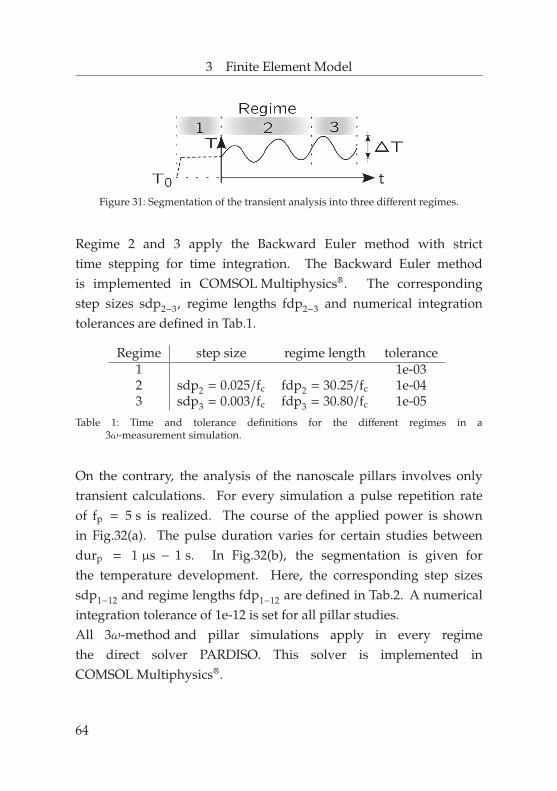
3 Finite Element Model
Figure 31: Segmentation of the transient analysis into three different regimes.
Regime 2 and 3 apply the Backward Euler method with stricttime stepping for time integration. The Backward Euler methodis implemented in COMSOL MultiphysicsR©. The correspondingstep sizes sdp2−3, regime lengths fdp2−3 and numerical integrationtolerances are defined in Tab.1.
Regime step size regime length tolerance1 1e-032 sdp2 = 0.025/fc fdp2 = 30.25/fc 1e-043 sdp3 = 0.003/fc fdp3 = 30.80/fc 1e-05
Table 1: Time and tolerance definitions for the different regimes in a3ω-measurement simulation.
On the contrary, the analysis of the nanoscale pillars involves onlytransient calculations. For every simulation a pulse repetition rateof fp = 5 s is realized. The course of the applied power is shownin Fig.32(a). The pulse duration varies for certain studies betweendurp = 1 µs − 1 s. In Fig.32(b), the segmentation is given forthe temperature development. Here, the corresponding step sizessdp1−12 and regime lengths fdp1−12 are defined in Tab.2. A numericalintegration tolerance of 1e-12 is set for all pillar studies.All 3ω-method and pillar simulations apply in every regimethe direct solver PARDISO. This solver is implemented inCOMSOL MultiphysicsR©.
64
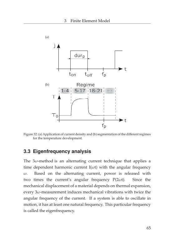
3 Finite Element Model
(a)
(b)
Figure 32: (a) Application of current density and (b) segmentation of the different regimesfor the temperature development.
3.3 Eigenfrequency analysis
The 3ω-method is an alternating current technique that applies atime dependent harmonic current I(ωt) with the angular frequencyω. Based on the alternating current, power is released withtwo times the current’s angular frequency P(2ωt). Since themechanical displacement of a material depends on thermal expansion,every 3ω-measurement induces mechanical vibrations with twice theangular frequency of the current. If a system is able to oscillate inmotion, it has at least one natural frequency. This particular frequencyis called the eigenfrequency.
65

3 Finite Element Model
Regime step size regime length1 sdp1 = 1e-03 fdp1 = 3e-032 sdp2 = 1.4e-06 fdp2 = 3.0014e-033 sdp3 = 2e-08 fdp3 = 3.00148e-034 sdp4 = 1e-09 fdp4 = 3.0015e-035 sdp5 = 1e-13 fdp5 = 3.001500001e-036 sdp6 = 1e-12 fdp6 = 3.00150001e-037 sdp7 = 1e-11 fdp7 = 3.0015001e-038 sdp8 = 1e-10 fdp8 = 3.001501e-039 sdp9 = 1e-09 fdp9 = 3.00151e-03
10 sdp10 = 1e-08 fdp10 = 3.0018e-0311 sdp11 = 1e-07 fdp11 = 3.003e-0312 sdp12 = 1e-06 fdp12 = 3.01e-0313 sdp13 = 1e-05 fdp13 = 3.5e-0314 sdp14 = 1e-04 fdp14 = 5.0e-0315 sdp15 = 1e-03 fdp15 = 1.0e-0216 sdp16 = 1e-02 fdp16 = 1.0e-0117 sdp17 = 1e-01 fdp17 = 1.0e+0018 sdp18 = 1e-02 fdp18 = 1.1e+0019 sdp19 = 1e-01 fdp19 = 1.5e+0020 sdp20 = 5e-01 fdp20 = 2.0e+0021 sdp21 = 1e+00 fdp21 = 5.0e+00
Table 2: Time definitions for the different regimes at nano/micro pillar studies.
The corresponding shape of motion is called the eigenmode [cf. 60, p.124]. However, if the excitation frequency equals the eigenfrequency ofthe used samples, a resonance catastrophe could occur. In resonance,a system exhibits especially for the case of small damping largeamplitudes in vibration. As result, mechanical displacements withlarge amplitude could occur which damage the small scale samples.To study the eigenfrequencies, the partial differential equation ofmotion of structural mechanics has to be solved.
66

3 Finite Element Model
In this work, damping is neglected so that
∇ ·σs + f = ρu , (3.59)
has to be solved [68, p. 11]. Here, double overdots denote the secondderivative with respect to time. Moreover, we assume the force vectorf to be zero to solve the problem of natural frequencies [cf. 128]. Toobtain the eigenfrequencies, we seek a solution in the harmonic formof
u = Υ · sin(ωt) , (3.60)
where Υ is the amplitude of motion [128, p. 12].It has to be mentioned, that the geometry and the boundary conditionscan have significant influence on the obtained eigenfrequencies. Therespective boundary conditions and geometric dimensions are givenfor each studied system in the respective section.
3.4 Mesh-block building system
Finite Element simulations always involve the challenge to find thebalance between accuracy and degrees of freedom. This concernsbesides careful considerations about the transient analysis also theFinite Element mesh. It is necessary to adopt the element size, elementshape and shape-functions for certain macroscopic and geometricalproblems. In this work, quad elements with linear shape functionsare used. However, in order to achieve high precision analysis, thiswork applies special geometry configurations to obtain a pre-definedmesh.31 Upon the geometry lines a mapped meshing method isapplied.
31The special geometry configurations are generated with Altair HyperWorksR©.
67
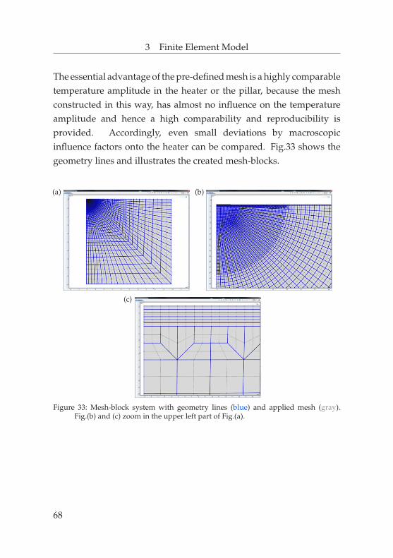
3 Finite Element Model
The essential advantage of the pre-defined mesh is a highly comparabletemperature amplitude in the heater or the pillar, because the meshconstructed in this way, has almost no influence on the temperatureamplitude and hence a high comparability and reproducibility isprovided. Accordingly, even small deviations by macroscopicinfluence factors onto the heater can be compared. Fig.33 shows thegeometry lines and illustrates the created mesh-blocks.
(a) (b)
(c)
Figure 33: Mesh-block system with geometry lines (blue) and applied mesh (gray).Fig.(b) and (c) zoom in the upper left part of Fig.(a).
68

4 Investigation of varying structures and
multiphysical couplings
4.1 Top down geometry
4.1.1 Heat source on bulk materials
This section examines several influence factors on a3ω-measurement for heat sources on bulk materials. First, avalidation of the used Finite Element Model is given for a quasisemi-infinite half space [cf. Fig.34(a)]. Afterwards, the substrate isreduced to realistic dimensions and various heat transfer conditionsfor the mount are studied [cf. Fig.34(b)]. Subsequently, we investigatestep by step the spatial extent of the heater and take into accountits material properties [cf. Fig.34(c)], the temperature dependentresistivity, three-dimensional heat conduction in the substrate,radiation, occurring surface roughness, the skin effect, and thermalexpansions and stresses. The following sections deal with the oxidesubstrate materials MgO, STO and YSZ.32
4.1.1.1 Validation of Finite Element ModelFirst of all, the solution of the Finite Element Model for the temperatureamplitude has to be validated by the fundamental solution of Eq.2.17from Cahill. To check the Finite Element Model by the semi-infinitehalf space solution of Cahill, a quasi semi-infinite half space with atremendous size of ds = 0.5 m is modeled.
32Find App.B for further information.
69

4 Investigation of varying structures and multiphysical couplings
h
Ωs
Γ
Γ1
Γ2
Γ3
Γ4
(a)
Γ
h
Ωs
4
Γ
Γ1 Γ3
Γ2
(b)
Γ
Ωs
4
Γ1 Γ3
Γ2ΩH
(c)
Figure 34: Considered systems for the Finite Element simulations: (a) Quasi semi-infinitehalf space; (b) real substrate size with heat transfer coefficient; (c) spatial heaterwith material properties.
The boundaries [cf. Fig.34(a)] Γ1−3 are adiabatic
Γ1−3 : κs/h∂Ts/h
∂n= 0 , (4.1)
while Γ4 is isothermal
Γ4 : T0 = 300 K . (4.2)
Here the released power per length is applied as heat flux boundarycondition (heat flux BC) at Γh for 0 ≤ x ≤ b so that
Γh : p =P0
2b·
12· (1 + cos(2ωt)) . (4.3)
The solution of Eq.2.17 and the Finite Element solution are comparedin Fig.35(a). Evidently, the solutions are almost congruent in the lowfrequency regime. For increasing frequency, there is a slight tendencyfor the Finite Element Model to obtain a greater temperature amplitudetowards the high frequency regime.
70

4 Investigation of varying structures and multiphysical couplings
0.00
0.05
0.10
0.15
0.20
100 101 102 103 104 105 106
∆T
[K]
Frequency fc [Hz]
Solution ofFES, quasi semi-infinite subs
(a)Eq.2.17
0.1789
0.1794
0.1799
0.1804
100
∆T
[K]
0.0845
0.0850
0.0855
103
Frequency fc [Hz]
0.0272
0.0274
0.0276
105
Mesh
1234567
(b)
Figure 35: (a) Validation of Finite Element solution (FES) and (b) a corresponding meshstudy. The degrees of freedom for Mesh 1 − 7 are 1281, 2923, 4106, 13454, 28581,49577 and 76310 respectively. The validation is calculated with Mesh 4. Thesystem properties are: P0/L = 5 W/m, 2b = 10 µm and MgO substrate.
Fig.35(b) shows a mesh study for several applied mesh-block systems.Mesh 4 is chosen as a reasonable compromise between the accuracyand the degrees of freedom because then, the Finite Element solutionyields an accuracy on the 4th decimal place. To guarantee this accuracy,an integration tolerance of 1e-05 is realized in COMSOL MultiphysicsR©.Consequently, it is now possible to compare temperature amplitudeswith this numerical precision.
4.1.1.2 Real substrate sizeSince a real substrate has a finite thickness [cf. Fig.34(b)], the heat flowfrom the substrate to the mount needs to be considered. Here, thisheat transfer is taken into account with a heat transfer coefficient (htc)so that
Γ4 : κs∂Ts
∂n− htc · (Ts − T0) = 0 . (4.4)
71

4 Investigation of varying structures and multiphysical couplings
The htc is defined as
htc =qn/S
Ts − T0, (4.5)
where qn/S indicates the flux per surface area. The boundaries Γ1−3
are adiabatic. First, an moderately-conductive substrate material isconsidered to study the influence of thermal contact to the mount atboundary Γ4. Fig.36(a) shows that a varying heat transfer coefficientcan have a significant influence on the temperature amplitude. Forinstance, even though the thermal penetration depth in STO is threetimes smaller than the substrate’s thickness, there is obviously aninfluence on ∆T at fc = 1 Hz with a corresponding q−1 = 0.0003 m[cf. Fig.21(a)]. However, the measured temperature amplitude isless affected for higher frequencies.33 This circumstance is given bythe fact, that the temperature amplitude does not vary for increasinghtc above frequencies of fc = 10 Hz. Thus, we propose to performmeasurements at frequencies above fc = 10 Hz.34
Furthermore, in Fig.36(a) and 36(b), the mean average temperaturesover the heater’s width are indicated for several htc for two differentsubstrates. For small htc values, thus poor thermal contact, themean average temperatures are tremendously higher than for largehtc values. Hence, sufficiently good thermal contact must be givento the substrate mount to avoid high system temperatures.Given the htc and frequency restriction, the solution of the temperatureamplitude for a quasi semi-infinite substrate and the real substrate sizeare almost coincident [cf. Fig.37].
33This result is consistent with Borca-Tasciuc’s solution for finite substrate thickness [cf.Sec.2.2.1].
34Also Zong et al. [173] propose to measure at least from 10 Hz but with respect to theheat spread in the heater’s length dimension [cf. Sec.4.1.1.6].
72

4 Investigation of varying structures and multiphysical couplings
0.50
0.55
0.60
0.65
0.70
0.75
0.80
0.85
0.90
100 101 102 103 104 105 106 107 108
∆T
[K]
Heat transfer coefficient [W/m2K]
1550 K
425 K
313 K
301.7 K
300.63 K 300.51 K
1 Hz1.5 Hz
2 Hz10 Hz
100 Hz
(a)
2.00
2.50
3.00
3.50
4.00
4.50
100 101 102 103 104 105 106 107 108
∆T
[K]
Heat transfer coefficient [W/m2K]
1553 K
428 K
315.3 K
304.1 K
303.0 K
302.9 K
1 Hz10 Hz
100 Hz
(b)
Figure 36: Influence of thermal contact to the mount for a (a) STO and (b) YSZ substratematerial. The dimension of the substrate is ds = 1 mm in height and 2 mm inwidth. Indicated are in addition the mean average temperatures over the heatsource width in time. The system properties are: P0/L = 5 W/m, 2b = 10 µm andthe ambient temperature is 300 K.
4.1.1.3 Geometrical variations of the heater and its materialpropertiesLike the substrate, a real heat source has a finite thickness [cf. Fiq.34(c)].Typically, a platinum (Pt) heater with thickness arround a = 100 nm isapplied. Including the spatial dimensions is of course accompanied byconsidering its thermal properties. Instead of a boundary condition,the heat is now released through the cross-sectional cut of the heater’sarea ΩH by Eq.3.3. The heat input for the heat flux BC model isevenly distributed over the heater width. However, actually theincoming heat can rearrange over the heater’s width and height. Thiscircumstance is taken into account in this section. Here, we set αin Eq.3.3 to zero, to develop step by step the different macroscopicinfluence factors.In Fig.38(a) and 38(b), a comparison between the BC model andthe more realistic heater is given for a highly-conductive andpoorly-conductive substrate material respectively. While the ∆T -linesare for a highly-conductive substrate material almost coincident, the
73
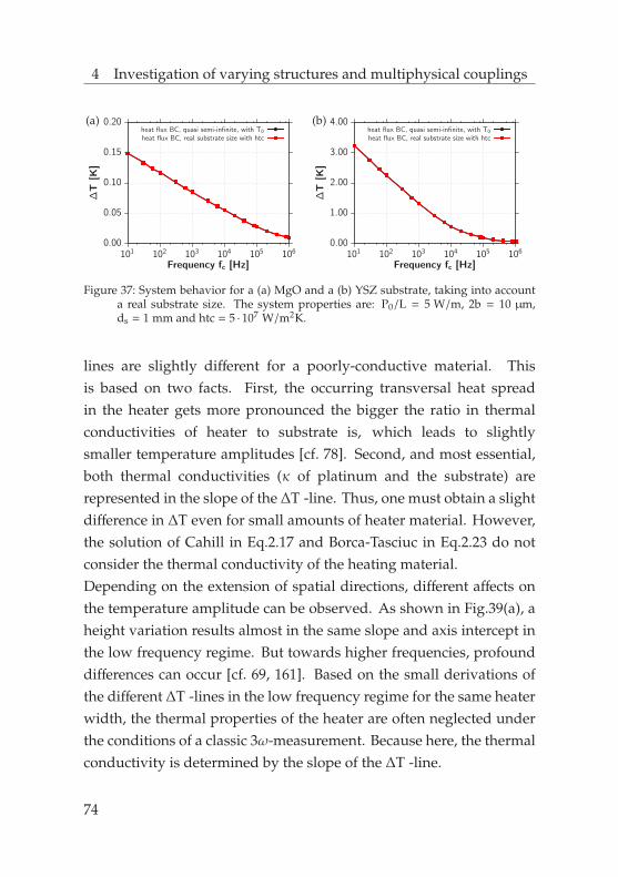
4 Investigation of varying structures and multiphysical couplings
0.00
0.05
0.10
0.15
0.20
101 102 103 104 105 106
∆T
[K]
Frequency fc [Hz]
heat flux BC, quasi semi-infinite, with T0
heat flux BC, real substrate size with htc
(a)
0.00
1.00
2.00
3.00
4.00
101 102 103 104 105 106
∆T
[K]
Frequency fc [Hz]
heat flux BC, quasi semi-infinite, with T0
heat flux BC, real substrate size with htc
(b)
Figure 37: System behavior for a (a) MgO and a (b) YSZ substrate, taking into accounta real substrate size. The system properties are: P0/L = 5 W/m, 2b = 10 µm,ds = 1 mm and htc = 5 · 107 W/m2K.
lines are slightly different for a poorly-conductive material. Thisis based on two facts. First, the occurring transversal heat spreadin the heater gets more pronounced the bigger the ratio in thermalconductivities of heater to substrate is, which leads to slightlysmaller temperature amplitudes [cf. 78]. Second, and most essential,both thermal conductivities (κ of platinum and the substrate) arerepresented in the slope of the ∆T -line. Thus, one must obtain a slightdifference in ∆T even for small amounts of heater material. However,the solution of Cahill in Eq.2.17 and Borca-Tasciuc in Eq.2.23 do notconsider the thermal conductivity of the heating material.Depending on the extension of spatial directions, different affects onthe temperature amplitude can be observed. As shown in Fig.39(a), aheight variation results almost in the same slope and axis intercept inthe low frequency regime. But towards higher frequencies, profounddifferences can occur [cf. 69, 161]. Based on the small derivations ofthe different ∆T -lines in the low frequency regime for the same heaterwidth, the thermal properties of the heater are often neglected underthe conditions of a classic 3ω-measurement. Because here, the thermalconductivity is determined by the slope of the ∆T -line.
74

4 Investigation of varying structures and multiphysical couplings
0.00
0.05
0.10
0.15
0.20
101 102 103 104 105 106
∆T
[K]
Frequency fc [Hz]
heat flux BC, real substrate size with htcspatial heater, real substrate size with htc
(a)
0.00
1.00
2.00
3.00
4.00
101 102 103 104 105 106
∆T
[K]
Frequency fc [Hz]
heat flux BC, real substrate size with htcspatial heater, real substrate size with htc
(b)
Figure 38: Influence of spatial heater and its material properties for a (a) MgO and (b)YSZ substrate. The system properties are: P/L = 5 W/m, 2b = 10 µm, a = 100 nm,ds = 1 mm and htc = 5 · 107 W/m2K.
0.00
0.20
0.40
0.60
0.80
101 102 103 104 105 106
∆T
[K]
Frequency fc [Hz]
a = 10 nma = 100 nm
a = 1000 nma = 2b = 10000 nm
(a)
0.00
0.20
0.40
0.60
0.80
101 102 103 104 105 106
∆T
[K]
Frequency fc [Hz]
2b = 5 µm2b = 10 µm2b = 20 µm2b = 50 µm
(b)
Figure 39: Influence of the heater (a) height and (b) width on the temperature amplitude.The system properties are: P/L = 5 W/m, Pt heater, 2b = 10 µm, a = 100 nm, STOsubstrate, ds = 1 mm and htc = 5 · 107 W/m2K.
A classic 3ω-measurement applies frequencies up to fc = 1000 Hz,moderately- to highly-conductive substrate materials and a smallheater thickness.On the contrary, a width variation results always in the same slope butdifferent axis intercepts in the low frequency regime [cf. Fig.39(b)].However, evidentially, high-precision analysis beyond the classicmeasuring configurations requires to take the heater properties intoaccount. This argument is even further supported in Sec.4.1.2.
75

4 Investigation of varying structures and multiphysical couplings
4.1.1.4 General temperature distribution for a heater substratesystemIn this section, the temperature distribution is examined in general.Therefore, time points are defined within one temperature cycle in thesteady state oscillation level in Fig.40.
Figure 40: Various time points within one temperature cycle.
First, the maximum and minimum temperatures within a temperatureamplitude are considered. The boundary conditions are the same thanin the previous section and the source term is given by Eq.3.3.Fig.41 shows the current temperature at the time points 2 and 4 .Here, the maximum and minimum temperatures at fc = 10 Hz arein each case higher and lower than for fc = 1 MHz. The lowest meantemperature remains at a higher level for fc = 1 MHz, while the systemcools down almost to ambient temperature for fc = 10 Hz. Drawing ahorizontal cut between the heater and the substrate along the heater’swidth and a vertical cut along the axis of symmetry, Fig.42 showsthe actual temperatures for the time points 1 − 5 . The horizontalcut in Fig.42(a) and 42(b) exhibits that the maximum temperature isalways below the center of the heater. This does not depend on thecurrent’s frequency. It illustrates furthermore, the higher minimumnmean average temperature at fc = 1 MHz. While the vertical cut inFig.42(c) shows clearly decreasing temperature trends for each timepoint without an overlap, the temperature lines in Fig.42(d) cross each
76

4 Investigation of varying structures and multiphysical couplings
(a) (b)
(c) (d)
Figure 41: Visualization of (a)(b) the maximum and (c)(d) minimum temperatures withina temperature cycle for fc = 10 Hz on the left and fc = 1 MHz on the right side.The system properties are: P0/L = 5 W/m, Pt heater, 2b = 10 µm, a = 100 nm,MgO substrate, ds = 1 mm and htc = 5 · 107 W/m2K.
other at a certain vertical depth. The crossing takes place at the thermalpenetration depth q−1, indicated by the black vertical line.
77

4 Investigation of varying structures and multiphysical couplings
300.000
300.050
300.100
300.150
300.200
300.250
−1 · 10−6 1 · 10−6 3 · 10−6 5 · 10−6
T[K
]
horizontal distance [m]
Time Point 12345
(a)
300.000
300.050
300.100
300.150
300.200
300.250
−1 · 10−6 1 · 10−6 3 · 10−6 5 · 10−6
T[K
]
horizontal distance [m]
Time Point 12345
(b)
300.000
300.050
300.100
300.150
300.200
300.250
−1 · 10−6 1 · 10−6 3 · 10−6 5 · 10−6
T[K
]
vertical depth [m]
Time Point 12345
(c)
300.075
300.080
300.085
300.090
300.095
300.100
−1 · 10−6 1 · 10−6 3 · 10−6 5 · 10−6
T[K
]
vertical depth [m]
q−1
Time Point 12345
(d)
Figure 42: Temperature distribution along a (a),(b) horizontal and (c),(d) vertical cut.The system properties are: P0/L = 5 W/m, Pt heater, 2b = 10 µm, a = 100 nm,MgO substrate, ds = 1 mm, htc = 5 · 107 W/m2K and fc = 10 Hz in (a),(c) andfc = 1 MHz in (b),(d).
4.1.1.5 Temperature dependent resistivity of the heaterThe analytic descriptions for the temperature amplitude by Cahill [28]and Borca-Tasciuc et al. [22] assume a constant power per length.However, since the electric resistivity is coupled with temperature,the dissipated power changes even within a temperature cycle. Thiscircumstance is incorporated with the linear temperature coefficient αinto Eq.3.3. The BC’s are like in the previous section.A comparison between a fix and a temperature dependent resistivityis shown in Fig.43. In general two factors change the temperatureamplitude.
78

4 Investigation of varying structures and multiphysical couplings
0.00
0.05
0.10
0.15
0.20
101 102 103 104 105 106
∆T
[K]
Frequency fc [Hz]
−1 · 10−4
−5 · 10−5
0 · 100
101 106∆
Tfi
x−∆
T
fix resistivitytemp dependent resistivity
(a)
0.00
1.00
2.00
3.00
4.00
101 102 103 104 105 106
∆T
[K]
Frequency fc [Hz]
−4 · 10−2
−2 · 10−2
0 · 100
101 106
∆T
fix−∆
T
fix resistivitytemp dependent resistivity
(b)
0.00
0.10
0.20
0.30
0.40
0.50
0.60
0.70
0.80
101 102 103 104 105 106
∆T
[K]
Frequency fc [Hz]
−2 · 10−3
−1 · 10−3
0 · 100
101 106
∆T
fix−∆
T
fix resistivitytemp dependent resistivity
(c)
0.00
2.00
4.00
6.00
8.00
101 102 103 104 105 106
∆T
[K]
Frequency fc [Hz]
−2 · 10−1
−1 · 10−1
0 · 100
101 106
∆T
fix−∆
T
fix resistivitytemp dependent resistivity
(d)
Figure 43: Influence of the temperature dependent electrical resistivity in the heater for a(a),(c) MgO and (b),(d) YSZ substrate. The system properties are: Pt heater, 2b =10 µm, a = 100 nm, ds = 1 mm, htc = 5 · 107 W/m2K and P/L = 5 W/m in (a),(b)and P/L = 20 W/m in (c),(d). The insets contain the difference in ∆T between a fix(∆T fix) and a temperature dependent resistivity (∆T ).
First, a poorly-conductive material leads to a higher ∆T than ahighly-conductive material [cf. Fig.43(b) and 43(a)]. Thus, thedifference is greater for poorly-conductive substrate materials. Second,a higher P/L increases the difference even more [cf. Fig.43(a) and43(c)]. The biggest difference is consequently given in Fig.43(d), wherethe models differ on the first digit after decimal place. However, it hasto be mentioned, that this represents the maximum in variation, sinceusually a 3ω-measurement takes place at lower P/L and especially fora ∆T around 1 K.
79

4 Investigation of varying structures and multiphysical couplings
4.1.1.6 Three-dimensional heat conduction in the substrateThe analytic descriptions for the temperature amplitude by Cahill [28]and Borca-Tasciuc et al. [22] consider a two-dimensional model. Tobe valid, the length of the heater must be much longer than its width,so that L 2b. However, even though this restriction is fulfilled,there is always heat conduction along the heater’s length dimension[cf. Fig.44].
x
y
z
Figure 44: Considered system for the Finite Element simulation for three-dimensionalheat conduction into the substrate.
In this section, every outer boundary is adiabatic except the substratemount, where a htc is considered. The dissipated power is givenby Eq.3.3. The resulting temperature amplitude in the heater isdetermined by Eq.3.13.Fig.45 shows the three-dimensional temperature distribution for thetime points 2 and 4 [cf. Fig.40]. Like in Sec.4.1.1.4, the maximumand minimum temperatures are for fc = 10 Hz always higher and lowerthan for fc = 1 MHz. Therefore, compare Fig.45(a) and 45(c) versusFig.45(b) and 45(d). Moreover, one can notice for both frequencies andtime points a temperature drop along the heater towards the outer end.This circumstance is illustrated in Fig.46. Here, the spatial dependenceof the temperature amplitude δT is plotted with the correspondingmaximum and minimum temperature in the inset.
80

4 Investigation of varying structures and multiphysical couplings
The cut is set along the z-axis below the center of the heater towardsthe outer edge of the substrate (z = 1 mm and L/2 = 0.5 mm). Acomparison of a highly-, moderately- and poorly-conductive substratematerial is given for fc = 10 Hz in Fig.46(a), 46(b) and 46(c). Indicatedby the green rectangle, the spatial temperature amplitude decreasestowards the heater’s end significantly earlier for highly-conductivethan for poorly-conductive materials. On the contrary, a frequencyincrease keeps the spatial temperature amplitude over a longerdistance constant. For this, compare Fig.46(b) versus 46(d).A comparison between the two-dimensional models of Cahill ofEq.2.17 and Borca-Tasciuc of Eq.2.23 and a two- and three-dimensionalFinite Element solution is given in Tab.3 for three different frequencies.
Solution Cahill Borca-Tasciuc FE-2D FE-3D∆T Eq.2.17 Eq.2.23
10 Hz 0.68859 K 0.68856 K 0.69507 K 0.67404 K100 Hz 0.51094 K 0.51085 K 0.52034 K 0.51360 K1 MHz 0.01861 K 0.01453 K 0.02265 K 0.02267 K
Table 3: Comparison of different solutions for a heater substrate system. The systemproperties are: P/L = 5 W/m, Pt heater, 2b = 10 µm, a = 100 nm, L/2 = 0.5 mm,STO substrate, ds = 1 mm and htc = 5 · 107 W/m2K.
According to Sec.4.1.1.1, the Finite Element solution is slightly abovethe analytic descriptions for two dimensions. However, a comparisonof the two- and three-dimensional Finite Element solution resultsin a smaller ∆T for the three-dimensional analysis than for thetwo-dimensional case. This is due to a heat flow along the z-directionin the heater and the substrate. Since the heater has not the length ofthe substrate’s width, the heater has its coolest cross-sectional cut atthe end of its length. This circumstance is illustrated in Fig.45 and 46.
81
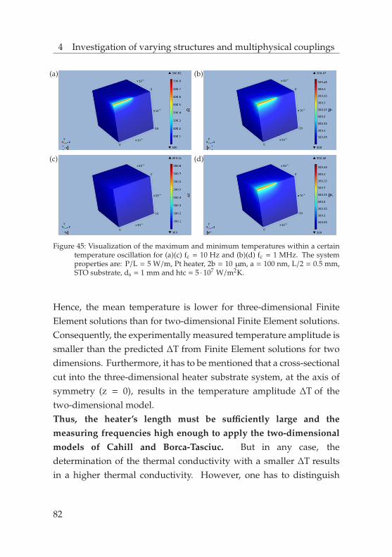
4 Investigation of varying structures and multiphysical couplings
(a) (b)
(c) (d)
Figure 45: Visualization of the maximum and minimum temperatures within a certaintemperature oscillation for (a)(c) fc = 10 Hz and (b)(d) fc = 1 MHz. The systemproperties are: P/L = 5 W/m, Pt heater, 2b = 10 µm, a = 100 nm, L/2 = 0.5 mm,STO substrate, ds = 1 mm and htc = 5 · 107 W/m2K.
Hence, the mean temperature is lower for three-dimensional FiniteElement solutions than for two-dimensional Finite Element solutions.Consequently, the experimentally measured temperature amplitude issmaller than the predicted ∆T from Finite Element solutions for twodimensions. Furthermore, it has to be mentioned that a cross-sectionalcut into the three-dimensional heater substrate system, at the axis ofsymmetry (z = 0), results in the temperature amplitude ∆T of thetwo-dimensional model.Thus, the heater’s length must be sufficiently large and themeasuring frequencies high enough to apply the two-dimensionalmodels of Cahill and Borca-Tasciuc. But in any case, thedetermination of the thermal conductivity with a smaller ∆T resultsin a higher thermal conductivity. However, one has to distinguish
82

4 Investigation of varying structures and multiphysical couplings
-0.04-0.020.000.020.040.060.080.100.120.140.160.18
0 0.0002 0.0004 0.0006 0.0008 0.001
δT[K
]
Length [m]
300.0
300.1
300.2
0 0.001
T[K
]Spatial temperature amplitude
(a)
fc = 10 Hz
-0.20-0.100.000.100.200.300.400.500.600.700.800.90
0 0.0002 0.0004 0.0006 0.0008 0.001
δT[K
]
Length [m]
300.0
300.5
301.0
0 0.001
T[K
]
Spatial temperature amplitude(b)
fc = 10 Hz
-1.00
0.00
1.00
2.00
3.00
4.00
0 0.0002 0.0004 0.0006 0.0008 0.001
δT[K
]
Length [m]
300.0
302.5
305.0
0 0.001
T[K
]
Spatial temperature amplitude(c)
fc = 10 Hz
-0.01
0.00
0.01
0.02
0.03
0 0.0002 0.0004 0.0006 0.0008 0.001
δT[K
]
Length [m]
300.0
300.2
300.5
0 0.001
T[K
]
Spatial temperature amplitude(d)
fc = 1 MHz
Figure 46: Influence of the heater’s length on the spatial temperature amplitude δT alongthe z-axis for a (a) MgO, (b),(d) STO and (c) YSZ substrate. The system propertiesare: Pt heater, 2b = 10 µm, a = 100 nm, ds = 1 mm and htc = 5 · 107 W/m2K. Theinsets contain the maximum and minimum temperature along the z-axis.
between a 2-pad and a 4-pad measurement. The simulated case wouldrepresent a 2-pad measurement since the temperature amplitude in theheater is determined over the same length then the structure is heated.Thus also at the edges, where the temperature amplitude decreases[cf. 12]. In comparison, a 4-pad measurement takes the voltage withina defined length of a longer heater structure. Hence, this effect isminimized. Although, the influence of the three-dimensional heatflow is shown by Jacquot et al. [78], this study is necessary within thiswork to understand the general heat flow required to develop a heatersubstrate platform and three-dimensional membrane systems.
83

4 Investigation of varying structures and multiphysical couplings
4.1.1.7 Radiation at the heater’s surfaceThe previous sections consider exclusively heat transfer by heatconduction. However, while heat transfer by convection is avoidedby performing a 3ω-measurement in vacuum, heat loss by radiation isalways existent [cf. Sec.1.2]. Although Cahill [28] already examinedthe influence of radiation, the effect on the temperature amplitudeis also included in this work. Thus we can study the influence ofradiation for the material combinations which we use in this work,and the effect of radiation can be compared quantitatively to the otherinfluence factors.In general, heat loss by radiation is affected by four different factors.First, a broad heater, compared to a narrow heater, offers a greatersurface for radiation to take place. Second, the more heat is conductedthrough the substrate, the less is going to be radiated. Thus, thethermal properties of the substrate limit indirectly the radiation losses.Third, heat loss by radiation is non-linear and changes with σbe(T4
−T40)
[cf. 35]. Hence, the ambient temperature T0 has crucial impact ontothe radiation losses. Here, σb is the Bolzmann constant and e isthe emissivity of the materials surface.35 To study the influence ofradiation loss on the temperature amplitude, we consider a linearizedapproximation at the outermost boundary [cf. Fig.34(c)] so that
Γ2 : κs/H∂Ts/H
∂n− σbeT3
0 · (Ts/H − T0) = 0 . (4.6)
This linearized approximation is just appropriate for small temperaturechanges [35, p. 18], like it is in a 3ω-measurement. Fourth, theapplied power per length defines basically the occurring temperatures.
35Find App.B. for detailed information about the Bolzmann constant and the emissivity.
84

4 Investigation of varying structures and multiphysical couplings
0.00
0.10
0.20
0.30
0.40
0.50
0.60
0.70
0.80
101 102 103 104 105 106
∆T
[K]
Frequency fc [Hz]
−1 · 10−4
0 · 1001 · 10−4
101 106∆T
ra−∆T
without radiationwith radiation, worst case e = 1
(a)
0.00
0.50
1.00
1.50
2.00
2.50
3.00
3.50
101 102 103 104 105 106
∆T
[K]
Frequency fc [Hz]
−1 · 10−2
0 · 1001 · 10−2
101 106
∆T
ra−∆T
without radiationwith radiation, worst case e = 1
(b)
0.00
0.10
0.20
0.30
0.40
0.50
0.60
0.70
0.80
101 102 103 104 105 106
∆T
[K]
Frequency fc [Hz]
−2 · 10−4
0 · 1002 · 10−4
101 106
∆T
ra−∆T
without radiationwith radiation, worst case e = 1
(c)
0.00
0.50
1.00
1.50
2.00
2.50
3.00
3.50
101 102 103 104 105 106
∆T
[K]
Frequency fc [Hz]
−5 · 10−4
0 · 1005 · 10−4
101 106
∆T
ra−∆T
without radiationwith radiation, worst case e = 1
(d)
Figure 47: Influence of heat loss by radiation at the heater’s boundaries for an ambienttemperature of (a),(b) 300 K and (c),(d) 1300 K. The system properties are: Ptheater, 2b = 10 µm, a = 100 nm, STO substrate, ds = 1 mm, htc = 5 · 107 W/m2Kand the emissivity is assumed to be e = 1. The applied power is P/L = 5 W/m in(a),(c) and P/L = 20 W/m in (b),(d). The insets contain the ∆T ra − ∆T differencebetween a system taking into account radiation (∆T ra) and without (∆T ).
Consequently, this interacts with the non-linear changes of T4.Boundary Γ1 and Γ3 are adiabatic and Γ4 considers the substrate mount,where a htc is taken into account [cf. Fig.34(c)]. The dissipated poweris given by Eq.3.3. Since the heater’s width and the substrate materialare quasi-fixed system quantities, the influence of ambient temperatureand applied power per length are studied in Fig.47. To maximize theinfluence of radiation, the emissivity is set to e = 1.
85

4 Investigation of varying structures and multiphysical couplings
While the difference in temperature amplitude (∆T ra − ∆T ) is almostnonexistent for room temperature [cf. Fig.47(a) and 47(b)], there isa slight difference for high temperatures [cf. Fig.47(c) and 47(d)].However, even for a high power per length and high temperature,the difference in temperature amplitude is first observed at the 4th
decimal place. Consequently, heat loss by radiation can be neglectedfor classic measuring configurations.
4.1.1.8 Surface roughnessAlso Half-Heusler alloys are nowadays subject of research forthermoelectrics. While the surface of STO, PCMO and MgO is ratherflat, special Half-Heusler materials develop a surface roughness onthe order of several nanometers [cf. 80, 81]. If the heater has thesurface’s shape, different heater width could occur. Fig.48 illustratesthese circumstances.
Γ
Ωs
4
Γ1 Γ3
Γ2ΩH
(a)
Γ
Ωs
4
Γ1 Γ3
Γ2ΩH
beff
(b)
Figure 48: Considered systems for the Finite Element simulation with (a) surfaceroughness and (b) an effective heater width.
Here, we investigate the influence of surface roughness for a peakheight of 20 nm on a 200 nm base. The boundaries Γ1−3 are adiabaticand Γ4 takes into account a htc. The dissipated power is given byEq.3.3. We study the difference between three different shapes of theheater.
86

4 Investigation of varying structures and multiphysical couplings
0.00
0.05
0.10
0.15
0.20
101 102 103 104 105 106
∆T
[K]
Frequency fc [Hz]
−1 · 10−4
0 · 1001 · 10−4
101 106
∆T−∆T
mod
smooth surfacesurface roughness
roughness with effective width
Figure 49: Influence of surface roughness on the cross-sectional cut of the heater. Awaved surface of 20 nm peaks on a 200 nm base is realized. The system propertiesare: Pt heater, 2b = 10 µm, a = 100 nm, MgO substrate, ds = 1 mm and htc =5 · 107 W/m2K. The insets contain the difference between a flat heater (∆T ) and asystem taking into account modifications of the heater due to a surface roughness(∆T mod).
The first shape is a rectangle with a smooth surface. The second shapehas the same heater width than the rectangle with the smooth surfacebut exhibits a surface roughness. The third shape considers the samepath length of the heater than the first shape, however exhibits a surfaceroughness too.A comparison between these models is given in Fig.49. Here,the inset shows a difference of the solutions (∆T − ∆T mod) on 4th
decimal place. Thus, a 3ω-measurement is almost unaffected bysuch small variations of the heater geometry. However, it has to bementioned that the present Finite Element simulations neglect interfaceresistances. But, if the heater is not perfectly connected to the materialbelow, interface resistances could become crucial.
87
4 Investigation of varying structures and multiphysical couplings
4.1.1.9 Skin effect in the heaterSince the 3ω-method is an alternating current technique, the currentdensity distribution has a tendency towards the boundary of thecross-sectional cut of the heater [cf. Sec.3.1.2]. Apart from materialparameters, this tendency depends on the frequency of the currentfc. In general, the characteristic skin depth can be calculatedwith Eq.A.324. Applying this formula results in a skin depth ofδskin = 0.1638 m and δskin = 0.0001638 m for fc = 10 Hz and fc = 1 MHzrespectively. Obviously, this spatial distance exceeds the heater’swidth 2b = 10 µm and height a = 100 nm by far, and thus almostno difference should occur in current density distribution along theheater’s spatial dimension. However, since we focus even on thesmallest changes in temperature amplitude, this effect is studied hereto examine the influence on ∆T .The boundaries Γ1−3 are adiabatic and Γ4 takes into account a htc. Thedissipated power is given by Eq.3.3. However, in this equation, thecurrent density is represented by the effective current density jeff ofEq.3.45.The new occurring current density distribution is shown in Fig.50 fortwo different heater widths and three different frequencies. While thereis almost no gradient observable for the heater width of 2b = 10 µmat fc = 10 kHz in Fig.50(a), the distribution changes slightly towardsthe outer edge of the heater for fc = 1 MHz in Fig.50(c) and 50(e). Onthe contrary, a heater width of 2b = 50 µm also comprises a differentdistribution at fc = 10 kHz [cf. Fig.50(b)]. Apparently, the distributiondoes not vary in the heater’s height for both given configurations[cf. 83]. Even if a tremendous heater with the dimensions of a =
2b = 50 µm would be applied for measurements, almost no gradientis observable in the density distribution at fc = 10 Hz [cf. Fig.51(a)].
88

4 Investigation of varying structures and multiphysical couplings
(a) (b)
(c) (d)
(e) (f)
Figure 50: Visualization of the current distribution for a heater width of 2b = 10 µm(a),(c),(e) and 2b = 50 µm (b),(d),(f) for 10 kHz, 100 kHz and 1 MHz respectively.The system properties are: P/L = 5 W/m, Pt heater, a = 100 nm, STO substrate,ds = 1 mm and htc = 5 · 107 W/m2K.
(a) (b)
Figure 51: Visualization of the current distribution in a squared heater for (a) 10 Hz and(b) 1 MHz. The system properties are: P/L = 5 W/m, Pt heater, dimensions ofa = 2b = 50 µm, STO substrate, ds = 1 mm and htc = 5 · 107 W/m2K.
On the contrary, at fc = 1 MHz, a gradient would occur in the directionof height and width [cf. Fig.51(b)] [cf. 64]. However, it has to bementioned that these heater dimensions are unlikely to be used for a3ω-measurement.
89

4 Investigation of varying structures and multiphysical couplings
0.00
0.05
0.10
0.15
0.20
0.25
0.30
0.35
0.40
104 105 106
∆T
[K]
Frequency fc [Hz]
0 · 100
5 · 10−3
1 · 10−2
104 106
∆T−∆T
sk
without skin effectwith skin effect
(a)
0.00
0.03
0.05
0.08
0.10
104 105 106
∆T
[K]
Frequency fc [Hz]
0 · 100
5 · 10−3
1 · 10−2
104 106
∆T−∆T
sk
without skin effectwith skin effect
(b)
Figure 52: Influence of the skin effect for a (a) narrow and a (b) broad heater. The systemproperties are: P/L = 5 W/m, Pt heater, a = 100 nm, STO substrate, ds = 1 mmand htc = 5 · 107 W/m2K. The insets contain the ∆T − ∆T sk difference betweena system with an equally distributed current density and a system taking intoaccount the skin effect in the heater.
The influence on the temperature amplitude is shown in Fig.52. Thedifference between a changed heating due to the skin effect and theassumption of equal distributed current density is shown in the insetfor a heater width of 2b = 10 µm in Fig.52(a) and for 2b = 50 µm inFig.52(b). Even though a different density distribution exists towardshigher frequencies, the effect of the changed heating is negligible inthe high frequency regime.
4.1.1.10 Thermal expansion and stressesThe measurement principle of the 3ω-method is based on heatproduction in the heater and dissipation into the investigated material.Analytic descriptions of Cahill and Borca-Tasciuc consider exclusivelyfixed geometries. However, a temperature change in a material isoften coupled with a mechanical deformation. Depending on thethermal expansion coefficients of the respective materials, the spatialdimension of the heater is subject to change.36
36Although we assume small deformations [cf. Sec.3.1.3], the influence of mechanicalexpansion on the temperature amplitude is investigated here.
90

4 Investigation of varying structures and multiphysical couplings
Hence, the power input is given through a continuously changingcross-sectional cut of the heater and thus, the current density variesthroughout a temperature cycle. To take into account the mechanicaldisplacement, the current density is calculated for every time step by
j =I0
(a + uy(a)) · (b + ux(b)), (4.7)
where, uy(a) and ux(b) are the mechanical displacements in height andwidth at the outer edge of the heater. Hence, the heat source term ofEq.3.3 writes now as
p = %0 · (1 + α · (T − T0)) ·( I0
(a + uy(a)) · (b + ux(b))
)2·
12· (1 + cos(2ωt)) .
(4.8)
This time-varying process is taken into account for two representativesubstrate materials (STO and YSZ) in Fig.53(a) and 53(b) respectively.The thermal conditions are the same as in the previous section.The conditions of the mechanical field are given in Sec.3.1.3. Sincethe thermal expansion coefficient (1/ K) depends on the relativelychanging temperature, this effect can be maximized always byapplying a higher power per length. Assuming the materials are inperfect mechanical contact, the difference in ∆T is at its maximum onlyat the 3rd decimal place for low frequencies. This difference levels off
for higher frequencies. For the previously given study, the mechanicalbehavior is visualized in Fig.54 for the maximum temperature at timepoint 2 in Fig.40. According to the thermal and mechanical boundaryconditions of Sec.3, the maximum displacements in x-direction areat the upper right edge of the cross-sectional cut of the system [cf.Fig.54(a)].
91
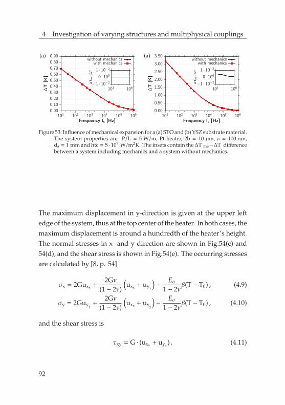
4 Investigation of varying structures and multiphysical couplings
0.00
0.10
0.20
0.30
0.40
0.50
0.60
0.70
0.80
0.90
101 102 103 104 105 106
∆T
[K]
Frequency fc [Hz]
−1 · 10−2
0 · 1001 · 10−2
101 106∆T
me−∆T
without mechanicswith mechanics
(a)
0.00
0.50
1.00
1.50
2.00
2.50
3.00
3.50
101 102 103 104 105 106
∆T
[K]
Frequency fc [Hz]
−1 · 10−2
0 · 1001 · 10−2
101 106
∆T
me−∆T
without mechanicswith mechanics
(a)
Figure 53: Influence of mechanical expansion for a (a) STO and (b) YSZ substrate material.The system properties are: P/L = 5 W/m, Pt heater, 2b = 10 µm, a = 100 nm,ds = 1 mm and htc = 5 · 107 W/m2K. The insets contain the ∆T me−∆T differencebetween a system including mechanics and a system without mechanics.
The maximum displacement in y-direction is given at the upper leftedge of the system, thus at the top center of the heater. In both cases, themaximum displacement is around a hundredth of the heater’s height.The normal stresses in x- and y-direction are shown in Fig.54(c) and54(d), and the shear stress is shown in Fig.54(e). The occurring stressesare calculated by [8, p. 54]
σx = 2Guxx +2Gν
(1 − 2ν)
(uxx + uyy
)−
Eσ1 − 2ν
β(T − T0) , (4.9)
σy = 2Guyy+
2Gν(1 − 2ν)
(uxx + uyy
)−
Eσ1 − 2ν
β(T − T0) , (4.10)
and the shear stress is
τxy = G · (uxy + uyx) . (4.11)
92

4 Investigation of varying structures and multiphysical couplings
(a) (b)
(c) (d)
(e) (f)
Figure 54: Visualization of the mechanical displacements and resulting stresses forthe maximum temperature within a certain oscillation [cf. Fig.40]. (a) is thedisplacement in x-direction, (b) is the displacement in y-direction, (c) is the stressin x-direction, (d) is the stress in y-direction and (e) is the shear stress in thex-y-plane. For the time point with maximum temperature, the distribution isillustrated in (f). The system properties are: fc = 10 Hz, P/L = 5 W/m, Pt heater,2b = 10 µm, a = 100 nm, STO substrate, ds = 1 mm and htc = 5 · 107 W/m2K.
For each, the maximum stress occurs again at the center of theheater. The absolute stress values are < 3 N/m2 which is severalorders of magnitude below critical stresses [cf. 6]. The correspondingtemperature distribution is shown in Fig.54(f).
93

4 Investigation of varying structures and multiphysical couplings
4.1.1.11 Eigenfrequency analysisIn this section, the eigenfrequencies are examined. Here, we consideronly heater substrate configurations where a spatial platinum heateris placed on top the respective substrates. The platinum heater hasa width of 10 µm and a height of 100 nm. Corresponding to theprevious sections, the oxide substrate materials MgO, STO and YSZ arestudied for a thickness of 1 mm. The system configuraion is shown inFig.34(c). While the boundaries Γ2−Γ4 are fully free to move, we set themechanical displacement only for the axis of symmetry in x-directionto zero so that
Γ1 : ux = 0 . (4.12)
First, the MgO substrate is considered. This substrate exhibits the firsteigenfrequency at ω = 1.56 MHz. However, this frequency must becompared to the thermal excitation and not to the excitation of theapplied electric current. In a 3ω-measurement, the thermal excitationequals the heating frequency 2ω. Hence, the obtained eigenfrequencyis already reached for ω/2. Thus, the first critical frequency for theMgO substrate is 0.780 MHz. The corresponding eigenform describesa flapping of the substrate symmetric to boundary Γ1. This eigenformis shown in Fig.55. Due to the boundary conditions, this is the firsteigenform for every substrate material. The STO substrate exhibitsthe first eigenfrequency at ω = 1.21 MHz and thus the first criticalfrequency for the STO substrate is 0.605 MHz. The YSZ substrateexhibits the first eigenfrequency at ω = 1.02 MHz and thus the firstcritical frequency for the YSZ substrate is 0.510 MHz. However,in a 3ω-measurement the substrate is always placed on a mount atboundary Γ4 and hence this boundary can not move as freely as weassumed it.
94

4 Investigation of varying structures and multiphysical couplings
Figure 55: Visualization of the eigenmode at the first eigenfrequency ω = 1.56 MHz foran MgO substrate.
In any case, the given eigenfrequencies indicate that for thesesubstrates, 3ω-measurements can be performed up to 0.5 MHzwithout a resonance catastrophe.
95

4 Investigation of varying structures and multiphysical couplings
4.1.2 Heat source on layer-substrate materials
This section examines the general system behavior for a heatsource on layer-substrate materials. First, monolayer configurationsare studied [cf. Fig.56(a)] and the solutions for the temperatureamplitude are compared to the descriptions of Lee and Cahill[99] and Borca-Tasciuc et al. [22]. The potential for anisotropicthermal conductivity determination is examined for highly-conductiveand poorly-conductive substrate materials. Afterwards, multilayerconfigurations are studied [cf. Fig.56(b) and 56(c)] for the generalsystem behavior and the influence of different layer thickness andsequence on the temperature amplitude.
Ωs
ΩH
Ωlay
dlay
(a)
Ωs
ΩH
Ωlay dlay2
dlay1
(b)
Ωs
ΩH
dlay2
dlay1
... Ωlay
(c)
Figure 56: Considered layered systems for the Finite Element simulations: (a) Heatsource on one layer; (b) on two layers; (c) on a multilayer stack.
96
4 Investigation of varying structures and multiphysical couplings
In this section, only temperature fields are considered. The boundariesΓ1−3 are adiabatic and Γ4 takes into account a htc [cf. Fig.27]. The powerinput is given by Eq.3.3.
4.1.2.1 Monolayer configurationsIn general, one must distinguish between two different layersubstrate configurations. On one hand, there can be a relativelypoorly-conductive layer material on top of a highly-conductivesubstrate material and on the other hand, the opposite configuration.First, the classic configuration with a relatively poorly-conductive layermaterial is considered. Here, the 3ω-method is especially convenientto determine the cross-plane thermal conductivity. However, eventhough a 3ω-measurement is performed within the boundaries of theoffset model [cf. Eq.2.30], the temperature amplitude is affected bythe in-plane heat spread. Therefore, Cahill and Lee [33] proposed acorrection value to take this fact into account and revised the offsetmodel. Conversely, the solution of Borca-Tasciuc et al. [22] takes thisfact analytically into account. Moreover, this solution accounts forthermal properties of the heater to describe the system behavior moreprecisely in the high frequency regime.A comparison between the solutions of the different models is givenin Fig.57(a). First, the low frequency regime is considered until afrequency of fc = 10 kHz. Up to this frequency, the offset model ofEq.2.31 is valid in general. In this regime, the corrected offset modelof Cahill [Eq.2.31 including Eq.2.33], the solutions of Borca-Tasciuc[Eq.2.24 and Eq.2.23], and the Finite Element solution are almostcoincident. Only the original offset model of Cahill [Eq.2.31], withoutthe effective heater width differs slightly.
97

4 Investigation of varying structures and multiphysical couplings
0.00
0.05
0.10
0.15
0.20
0.25
0.30
0.35
0.40
101 102 103 104 105 106 107 108
∆T
[K]
Frequency fc [Hz]
0.200.230.250.28
101 102
Solution ofSolution ofSolution ofSolution ofFES including all mat. prop.
(a)Eq.2.31Eq.2.31+Eq.2.33Eq.2.24Eq.2.23
(b)
Figure 57: (a) Influence of in-plane heat spread and of heater properties in the highfrequency regime. (b) The corresponding temperature distribution illustrates theprofound temperature drop below the heater at fc = 10 Hz. The system propertiesare: P/L = 5 W/m, Pt heater, 2b = 10 µm, a = 100 nm, PCMO layer, dlay =
400 nm, isotropic layer, MgO substrate, ds = 1 mm and htc = 5 · 107 W/m2K.
Since the slight in-plane heat spread generally lowers the temperatureamplitude, this ∆T-line is slightly above the other four solutions. Theinset contains a scope of the temperature amplitude solutions between10 Hz and 100 Hz. Here the analytic solutions agree even betterwith the Finite Element solution than for the substrate validation inSec.4.1.1.1.On the contrary, a comparison in the high frequency regime revealssignificant differences. Since the offset model treats the layer as aone-dimensional resistor and thus does not include the frequencydependence of the layer into the solution, the offset model solutionsmust tend to a remaining temperature amplitude even for an infinitefc [cf. Fig.24]. In contrast, the solutions of Borca-Tasciuc of Eq.2.24 andEq.2.23 decrease significantly towards fc = 100 MHz. The solution ofEq.2.24, without the heater properties, remains for higher frequencies,at considerably larger temperature amplitudes than the solution ofEq.2.23 and the Finite Element solution. The significant decrease of∆T at fc = 10 MHz is due to the thermal penetration depth.
98

4 Investigation of varying structures and multiphysical couplings
0.00
0.05
0.10
0.15
0.20
0.25
0.30
0.35
101 102 103 104 105 106
∆T
[K]
Frequency fc [Hz]
unit=[J/kgK] cp = 48cp = 480cp = 4800
(a)
0.00
0.05
0.10
0.15
0.20
101 102 103 104 105 106
∆T
[K]
Frequency fc [Hz]
unit=[J/kgK] cp = 54.4cp = 544cp = 5440
(b)
Figure 58: Influence of a thermal mass variation on the temperature amplitude for an(a) PCMO layer and an (b) STO layer. The system properties are: P/L = 5 W/m,Pt heater, a = 100 nm, 2b = 10 µm, dlay = 400 nm, MgO substrate, ds = 1 mm,htc = 5 · 107 W/m2K.
Here, the penetration depth is on the order of the layer’s thickness.However, if the thermal mass (ρ · cp) of the heater is consideredadditionally in Borca-Tasciuc’s solution [Eq.2.23], the ∆T -linedecreases already at frequencies around fc = 300 kHz. This is due tothe thermal wave, which interacts now significantly with the thermalproperties of the layer and the heater. The Finite Element solutionconsiders in contrast to the analytic descriptions all material propertiesof the heater. Since only the solution of Eq.2.23 takes into accountthermal porperties of the heater, this ∆T -line is the closest to theFinite Element solution. Although the solutions of Borca-Tasciuccan be seen as bounds from above and below, the Finite ElementModel helps to understand the ∆T evolution in the high frequencyregime. Furthermore, it demonstrates the necessity of Finite Elementsimulations in terms of high precision analysis for new measuringmethods. Moreover, this result supports the assumption of neglectingthe thermal properties of the heater in the low frequency regime forclassic layer substrate geometries and configurations.
99

4 Investigation of varying structures and multiphysical couplings
On the contrary, the question arises how a thermal mass variation ofthe layer material takes an influence on the temperature amplitude. Tostudy the influence on ∆T, the original thermal mass of an PCMO andSTO layer is varied by a factor of ten. Hence three different cases arisefor both materials. The resulting temperature amplitudes are shown inFig.58. Evidently, the thermal mass of the layer material influencesthe temperature amplitude exclusively for higher frequencies.The actual temperature distribution for the 400 nm thick PCMO layeron top the MgO substrate is shown in Fig.57(b) for the time point 2 inFig.40. Even though a slight in-plane heat spread is present in the layer,a strong pronounced vertical temperature drop below the heater exists.Based on this temperature distribution, the offset model is justified.On one hand, the in-plane heat spread is undesired for the cross-planethermal conductivity determination. One the other hand, the in-planeheat spread can be used to determine the in-plane thermal conductivity.As mentioned in Sec.2.2.2, some groups applied narrow heaters todetermine the in-plane thermal conductivity for relatively thick andhighly-conductive materials by this in-plane heat spread. However,the materials investigated in this work are thin and poorly-conductive.The sensitivity on the temperature amplitude is shown in Fig.59 fortremendous varying cross- and in-plane thermal conductivities. In thiswork, sensitivity is defined as significant derivation from the isotropiccase of the ∆T -line. This includes different slopes and changingaxis-intercepts at various frequencies. Numerically, changes can beobserved easily, but the value changes in the temperature amplitudemust significantly exceed the measurement error in experiments. Themeasurement error of the experimental setup, used by our projectpartners, is determined to be around 5% [cf. 164].
100

4 Investigation of varying structures and multiphysical couplings
0.000.050.100.150.200.250.300.350.400.450.50
101 102 103 104 105 106
∆T
[K]
Frequency fc [Hz]
unit=[W/mK] κin = 0.158 κcrs = 1.58κin = 15.8 κcrs = 1.58κin = 1.58 κcrs = 1.58κin = 1.58 κcrs = 15.8
(a)
0.00
0.05
0.10
0.15
0.20
0.25
0.30
0.35
101 102 103 104 105 106
∆T
[K]
Frequency fc [Hz]
unit=[W/mK] κin = 0.158 κcrs = 1.58κin = 15.8 κcrs = 1.58κin = 1.58 κcrs = 1.58κin = 1.58 κcrs = 15.8
(b)
0.00
0.05
0.10
0.15
0.20
101 102 103 104 105 106
∆T
[K]
Frequency fc [Hz]
unit=[W/mK]κin = 0.158 κcrs = 1.58κin = 15.8 κcrs = 1.58κin = 1.58 κcrs = 1.58κin = 1.58 κcrs = 15.8
(c)
0.00
0.05
0.10
0.15
0.20
0.25
101 102 103 104 105 106
∆T
[K]
Frequency fc [Hz]
unit=[W/mK] κin = 1.0305 κcrs = 10.305κin = 103.05 κcrs = 10.305κin = 10.305 κcrs = 10.305κin = 10.305 κcrs = 103.05
(d)
Figure 59: Sensitivity for the anisotropic thermal transport. Changes in ∆T for a PCMOlayer including a (a) narrow 2b = 5 µm, (b) intermediate 2b = 10 µm and (c)broad 2b = 50 µm heater width. Changes in ∆T for a STO layer including an(d) intermediate heater width for 2b = 10 µm. The system properties are: P/L =5 W/m, Pt heater, a = 100 nm, dlay = 400 nm, MgO substrate, ds = 1 mm, htc =
5 · 107 W/m2K.
In Fig.59(a),59(b) and 59(c), different heater widths are applied onto athin poorly-conductive PCMO layer. To investigate the sensitivity forthe anisotropic thermal conductivities, the isotropic case is varied bya factor of ten. Hence five different cases arise. The case of extremelypoorly-conductive cross-plane thermal conductivity is neglected inFig.59.
101

4 Investigation of varying structures and multiphysical couplings
Except for moderately- and highly-conductive cross-plane thermalconductivities, only small differences occur in the ∆T -lines for anarrow, ‘normal’ and broad heater width [cf. Fig.59(a), 59(b) and59(c)]. Also the anisotropic variation of an moderately-conductive STOlayer results only in small differences in the ∆T -lines [cf. Fig.59(d)].Moreover, here the absolute values of the temperature amplitudes arealready small and the occurring differences in the ∆T -lines comparedto the tremendous variations of the thermal conductivities are evensmaller.For classic systems with a highly-conductive substrate, one candistinguish clearly between the influence of thermal conductivity andthermal mass of the layer on the temperature amplitude. Because here,a variation of the anisotropic thermal conductivity results in a constantslope until the thermal penetration depth is on the order of the layer.Moreover, since the slope is the same, but the axis intercept changes,the offset model can be applied in general, if the variations in ∆T aregreater than the measurement accuracies. The ratio of the isotropicthermal conductivity of layer to substrate are for the PCMO-MgOsystem κlay/κs ≈ 0.03 and for the STO-MgO system κlay/κs ≈ 0.18. If aPCMO layer would be applied onto a STO substrate, the ratio wouldbe κlay/κs ≈ 0.15. In this case, the offset model could also be used todetermine the cross-plane thermal conductivity.The opposite layer substrate configuration, with a poorly-conductivesubstrate, results in a completely different system behavior. Becausehere, a comprehensive influence of the thermal conductivity andthermal mass, thus the thermal diffusivity, is present over the wholefrequency regime. For these systems, the slope and axis interceptchange continuously. Here, a classic linear regime does not exist.This system behavior is shown in Fig.60(a) for an STO layer and inFig.60(b) for an PCMO layer for various layer thicknesses.
102

4 Investigation of varying structures and multiphysical couplings
0.00
0.50
1.00
1.50
2.00
2.50
3.00
3.50
101 102 103 104 105 106
∆T
[K]
Frequency fc [Hz]
dlay=100nmdlay=400nm
dlay=1000nm
(a)
0.00
0.50
1.00
1.50
2.00
2.50
3.00
3.50
101 102 103 104 105 106
∆T
[K]
Frequency fc [Hz]
dlay=100nmdlay=400nm
dlay=1000nm
(b)
Figure 60: Non-offest system behaviour for a (a) STO and (b) PCMO layer at variousheights. The system properties are: P/L = 5 W/m, Pt heater, a = 100 nm, 2b =10 µm, YSZ substrate, ds = 1 mm, htc = 5 · 107 W/m2K.
Hence, there is also no clearly defined offset or downshift dueto the STO and PCMO layer in the ∆T -line. As consequence,the cross-plane thermal conductivity cannot be determined bythe solution of Cahill and Lee [33] under these circumstances.However, since we are especially interested in the anisotropic thermalconductivity, the poorly-conductive substrate is further investigated.The sensitivity for the anisotropic thermal conduction is shownin Fig.61. Although we investigate tremendous variations in theanisotropic thermal conductivity, just two cases vary significantlyfrom the isotropic case. The highly-conductive in-plane case forSTO [Fig.61(a)] and the poorly-conductive cross-plane case for PCMO[cf. Fig.61(b)]. Even though the influence on the temperatureamplitude of the in-plane thermal conductivity can be increasedby a narrow heater, the YSZ substrate is also rather insensitivefor poorly-conductive in-plane thermal conductivities. Moreover,the application of poorly-conductive substrates would require alsomeasurements with a highly-conductive substrate to determine alsothe cross-plane thermal conductivity first.
103

4 Investigation of varying structures and multiphysical couplings
0.00
0.50
1.00
1.50
2.00
2.50
3.00
3.50
101 102 103 104 105 106
∆T
[K]
Frequency fc [Hz]
unit=[W/mK] κin = 1.0305 κcrs = 10.305κin = 103.05 κcrs = 10.305κin = 10.305 κcrs = 1.0305κin = 10.305 κcrs = 10.305κin = 10.305 κcrs = 103.05
(a)
0.00
1.00
2.00
3.00
4.00
5.00
101 102 103 104 105 106
∆T
[K]
Frequency fc [Hz]
unit=[W/mK] κin = 0.158 κcrs = 1.58κin = 15.8 κcrs = 1.58κin = 1.58 κcrs = 0.158κin = 1.58 κcrs = 1.58κin = 1.58 κcrs = 15.8
(b)
Figure 61: Sensitivity for the anisotropic thermal conduction for a (a) STO and (b) PCMOlayer. The system properties are: P/L = 5 W/m, Pt heater, a = 100 nm, 2b =10 µm, dlay = 400 nm, YSZ substrate, ds = 1 mm, htc = 5 · 107 W/m2K.
By this process, several unknown conditions are introduced by eachmeasurement so that the determination of the thermal conductivityis adversely affected. Consequently, this work aspires to determinethe in-plane and cross-plane thermal conductivity within onemeasurement for even thinner layers. Therefore, new measurementconfigurations are still necessary. For this reason, this work focusesalso on the bottom electrode and membrane geometries in sectionSec.4.2 and Sec.4.3, respectively.
4.1.2.2 Multilayer configurations
Multilayer systems are configurations with at least two individuallayers. The term multilayer is not specific about the layer’s thickness.However, new thermoelectric material properties are expected atlength scales around several nanometers for each layer thickness. Here,especially a new emergent thermal conductivity arises. But since thejoint project is also interested in layer thicknesses up to several hundrednanometers, the influence of layer thickness and stacking sequence isinvestigated here.
104
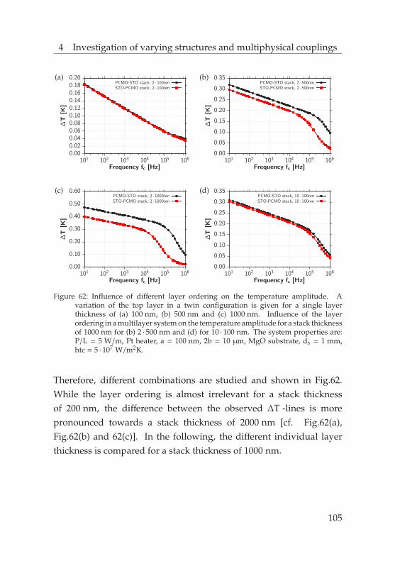
4 Investigation of varying structures and multiphysical couplings
0.000.020.040.060.080.100.120.140.160.180.20
101 102 103 104 105 106
∆T
[K]
Frequency fc [Hz]
PCMO-STO stack, 2 · 100nmSTO-PCMO stack, 2 · 100nm
(a)
0.00
0.05
0.10
0.15
0.20
0.25
0.30
0.35
101 102 103 104 105 106
∆T
[K]
Frequency fc [Hz]
PCMO-STO stack, 2 · 500nmSTO-PCMO stack, 2 · 500nm
(b)
0.00
0.10
0.20
0.30
0.40
0.50
0.60
101 102 103 104 105 106
∆T
[K]
Frequency fc [Hz]
PCMO-STO stack, 2 · 1000nmSTO-PCMO stack, 2 · 1000nm
(c)
0.00
0.05
0.10
0.15
0.20
0.25
0.30
0.35
101 102 103 104 105 106
∆T
[K]
Frequency fc [Hz]
PCMO-STO stack, 10 · 100nmSTO-PCMO stack, 10 · 100nm
(d)
Figure 62: Influence of different layer ordering on the temperature amplitude. Avariation of the top layer in a twin configuration is given for a single layerthickness of (a) 100 nm, (b) 500 nm and (c) 1000 nm. Influence of the layerordering in a multilayer system on the temperature amplitude for a stack thicknessof 1000 nm for (b) 2 · 500 nm and (d) for 10 · 100 nm. The system properties are:P/L = 5 W/m, Pt heater, a = 100 nm, 2b = 10 µm, MgO substrate, ds = 1 mm,htc = 5 · 107 W/m2K.
Therefore, different combinations are studied and shown in Fig.62.While the layer ordering is almost irrelevant for a stack thicknessof 200 nm, the difference between the observed ∆T -lines is morepronounced towards a stack thickness of 2000 nm [cf. Fig.62(a),Fig.62(b) and 62(c)]. In the following, the different individual layerthickness is compared for a stack thickness of 1000 nm.
105

4 Investigation of varying structures and multiphysical couplings
While an individual layer thickness of dlay = 500 nm results in twoclearly distinct ∆T -lines, the ∆T -lines are close to each other foran individual layer thickness of dlay = 100 nm [cf. Fig.62(b) andFig.62(d)]. Thus, the individual layer thickness should be as thinas possible to apply the offset model of Cahill. The reason for thissystem behavior is the in-plane heat spread in the layer below theheater. Shin et al. [144] also observed this upper layer influence.Without the in-plane heat spread, the ∆T -lines would be coincidentuntil the thermal penetration depth is on the order of the stackthickness. In this case, the cross-plane thermal conductivity couldbe determined with the offset model without an influence of thelayer ordering. However, a transition between an individual layerinfluence and a new representative material affects the temperatureamplitude measurements differently. This transition depends besideseach respective layer thickness also on the heater’s width and themeasuring frequency. But, it can be concluded from Fig.62(d), thatthe in-plane heat spread from the upper layer can be neglected fora poorly-conductive stack with a total thickness of dlaytot
≤ (2b)/10and an individual layer thickness of dlay < 100 nm.Thus, it is rather inappropriate to model each layer under thesecircumstances. Here, a new representative layer package canbe regarded for the Finite Element simulations to represent thestack. Consequently, anisotropic thermal conductivity variations ofa multilayer package are comparable with the monolayer studies ofSec.4.1.2.1.
106

4 Investigation of varying structures and multiphysical couplings
4.2 Bottom electrode geometry
A possible new geometry for the 3ω-method is the bottom electrodegeometry with the so-called heater substrate platform [cf. Fig.26].37
A main advantage would be the improved reproducibility ofthe corresponding measurements, as there are equal heat transferconditions to the substrate for each investigated material to becharacterized. Before a heater substrate platform can be appliedfor nanostructured samples, one must understand the whole systembehavior. Thus, the following section examines the general ∆T -linebehavior for bulk-like materials first. Subsequently, full covering thinfilms are studied. Afterwards patterned multilayers are consideredand compared to the classic geometry configuration.Every subsequent section on the bottom electrode considers the samethermal boundary conditions. Except the substrate mount, every outerboundary is considered to be adiabatic. The substrate mount takesinto account a htc to develop a realistic system behavior. The liberatedpower is given by Eq.3.3.
4.2.1 Bulk-like materials
In this section, three different geometry configurations areinvestigated. First, only thermal contact is given over the boundariesof the heater [cf. Fig.63(a)]. This geometry represents an ideal caseto study the influence of either thermal conductivity or thermal massvariations on the temperature amplitude. The next step considers amore realistic case. Here, the placed material above the heater substrateplatform also has spatial contact next to the heater [cf. Fig.63(b)].
37The bottom electrode concept is the basic idea of Ch. Jooss, Institute of MaterialsPhysics, University of Gottingen.
107
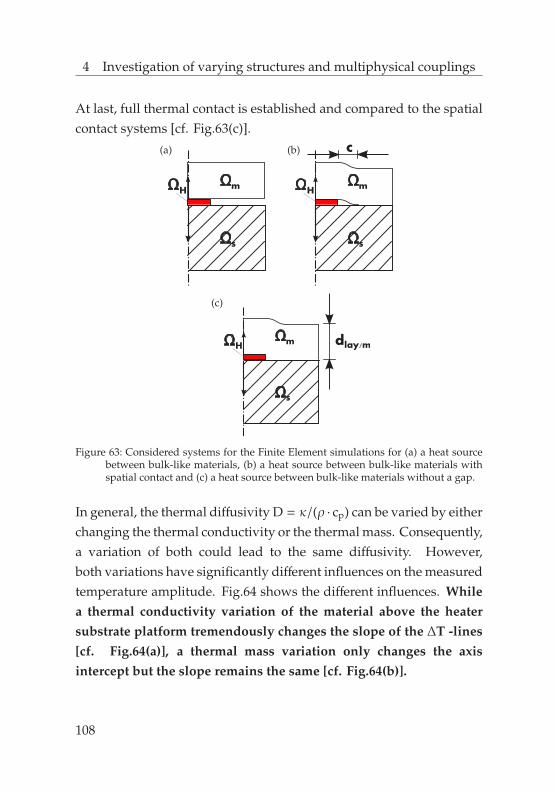
4 Investigation of varying structures and multiphysical couplings
At last, full thermal contact is established and compared to the spatialcontact systems [cf. Fig.63(c)].
Ωs
ΩHΩm
(a)
Ωs
ΩHΩm
c(b)
Ωs
ΩHΩm dlay/m
(c)
Figure 63: Considered systems for the Finite Element simulations for (a) a heat sourcebetween bulk-like materials, (b) a heat source between bulk-like materials withspatial contact and (c) a heat source between bulk-like materials without a gap.
In general, the thermal diffusivity D = κ/(ρ · cp) can be varied by eitherchanging the thermal conductivity or the thermal mass. Consequently,a variation of both could lead to the same diffusivity. However,both variations have significantly different influences on the measuredtemperature amplitude. Fig.64 shows the different influences. Whilea thermal conductivity variation of the material above the heatersubstrate platform tremendously changes the slope of the ∆T -lines[cf. Fig.64(a)], a thermal mass variation only changes the axisintercept but the slope remains the same [cf. Fig.64(b)].
108
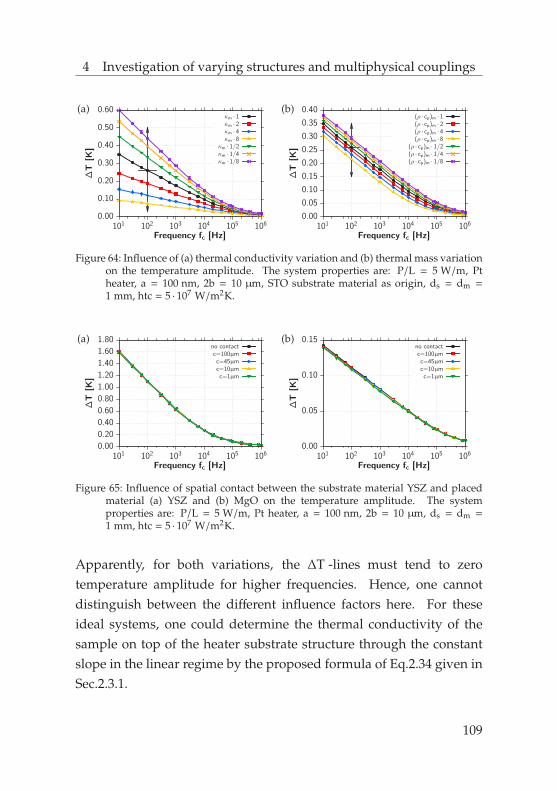
4 Investigation of varying structures and multiphysical couplings
0.00
0.10
0.20
0.30
0.40
0.50
0.60
101 102 103 104 105 106
∆T
[K]
Frequency fc [Hz]
κm · 1κm · 2κm · 4κm · 8
κm · 1/2κm · 1/4κm · 1/8
(a)
0.00
0.05
0.10
0.15
0.20
0.25
0.30
0.35
0.40
101 102 103 104 105 106
∆T
[K]
Frequency fc [Hz]
(ρ · cp)m · 1(ρ · cp)m · 2(ρ · cp)m · 4(ρ · cp)m · 8
(ρ · cp)m · 1/2(ρ · cp)m · 1/4(ρ · cp)m · 1/8
(b)
Figure 64: Influence of (a) thermal conductivity variation and (b) thermal mass variationon the temperature amplitude. The system properties are: P/L = 5 W/m, Ptheater, a = 100 nm, 2b = 10 µm, STO substrate material as origin, ds = dm =1 mm, htc = 5 · 107 W/m2K.
0.00
0.20
0.40
0.60
0.80
1.00
1.20
1.40
1.60
1.80
101 102 103 104 105 106
∆T
[K]
Frequency fc [Hz]
no contactc=100µmc=45µmc=10µmc=1µm
(a)
0.00
0.05
0.10
0.15
101 102 103 104 105 106
∆T
[K]
Frequency fc [Hz]
no contactc=100µmc=45µmc=10µmc=1µm
(b)
Figure 65: Influence of spatial contact between the substrate material YSZ and placedmaterial (a) YSZ and (b) MgO on the temperature amplitude. The systemproperties are: P/L = 5 W/m, Pt heater, a = 100 nm, 2b = 10 µm, ds = dm =1 mm, htc = 5 · 107 W/m2K.
Apparently, for both variations, the ∆T -lines must tend to zerotemperature amplitude for higher frequencies. Hence, one cannotdistinguish between the different influence factors here. For theseideal systems, one could determine the thermal conductivity of thesample on top of the heater substrate structure through the constantslope in the linear regime by the proposed formula of Eq.2.34 given inSec.2.3.1.
109

4 Investigation of varying structures and multiphysical couplings
0.00
0.50
1.00
1.50
2.00
101 102 103 104 105 106
∆T
[K]
Frequency fc [Hz]
dmat=dsubsdmat=dsubs/4dmat=dsubs/16dmat=dsubs/64
dmat=dsubs/256dmat=dsubs/2048
Figure 66: Influence on the temperature amplitude for decreasing material thickness ontop. The system properties are: P/L = 5 W/m, Pt heater, a = 100 nm, 2b = 10 µm,MgO material on top, ds = 1 mm, htc = 5 · 107 W/m2K.
However, these ideal systems are rather difficult to manufacture. Inmost experiments, the sample on top would probably also be inthermal contact with the substrate material [cf. Fig.63(b)]. Sincethe thermal conductivity of both materials is contained in the slopeof the ∆T -line, the maximum difference is given for a high contrastin thermal conductivities. In Fig.65(a), the same poorly-conductivesubstrate material is taken as sample material on top so that κm/κs = 1.In this case, the obtained ∆T -lines are coincident for various contactdistances c. On the contrary, for a contrast of κm/κs ≈ 30, a slightdifference can be observed even though the actual material parametersremain the same [cf. Fig.65(b)]. Consequently, a precise determinationof the thermal conductivity of the investigated material also requiresthe distance information for these configurations.The previous studies assume a bulk-like material on top. However,decreasing the thickness of the material [cf. Fig.63(c)] resultsin completely different ∆T -lines. The thickness influence of theplaced material on the ∆T -lines is shown in Fig.66. For decreasingmaterial thickness, the temperature amplitude increases significantly.Furthermore, thin materials on top lead to a continuously changingslope over the whole frequency regime.
110

4 Investigation of varying structures and multiphysical couplings
4.2.2 Thin layers
Decreasing the thickness of the placed materials results in thin coveringlayers [cf. Fig.67].
Ωs
ΩHΩlay
dlay
Figure 67: Considered system for the Finite Element simulations for a thin covering layeron top. The dash line indicates contour shape variations of the layer at the outeredge of the heater.
For bulk-like materials on top, the thermal conductivity is clearlyrepresented in the slope of the ∆T -line [cf. Sec.4.2.1]. For such asystem, a high contrast in thermal conductivities from the materialon top to the substrate would be ideal to determine the thermalconductivity of the investigated material. However, in case ofthin layers, the present thermal mass of the placed material israther small in comparison to the substrate material. Applying athin poorly-conductive layer material on top of a highly-conductivesubstrate material results in almost no change for the obtained ∆T -line.This is due to the small present thermal mass and the relatively highthermal resistance of the layer material in comparison to the substratematerial. Here, a tremendous amount of heat is conducted throughthe substrate. Hence, the influence of the thin layer on the temperatureamplitude is rather small. To increase the absolute temperatureamplitude and thus slight changes in the ∆T -line due to the layer,one must choose a poorly-conductive substrate material.
111

4 Investigation of varying structures and multiphysical couplings
In the following, the influence of the layer’s contour shape, thesensitivity for moderately- and poorly-conductive layers and theinfluence of anisotropic thermal conductivity of the layer is examinedon the temperature amplitude. First, the contour shape is considered.To maximize an eventual influence, a thin layer is applied. Fig.68shows the ∆T -lines for three different shape variations at the outeredge of the heater [cf. Fig.67]. Apparently, the ∆T -lines are coincidentand thus, the contour shape can be neglected. Second, the sensitivityfor an moderately- (STO) and poorly-conductive (PCMO) layer on topof the YSZ substrate is considered in Fig.69(a) and 69(b), respectively.While a difference occurs for the STO layer, there is almost no differencein the ∆T -lines for the PCMO layer, even though the layer thicknessis varied over a wide range. Third, an anisotropy variation [cf.Fig.70] bares, that even tremendous variations of the cross-planethermal conductivity are absolutely not detectable. On the contrary, ahighly-conductive in-plane thermal conductivity could be determinedfor both layer configurations. However, since thermoelectric materialsare expected to be poorly-conductive, these two cases are rather lessimportant for the anisotropy determination. According to the studiesfor bulk-like materials, the question arises whether additional materialabove the layer could emphasize the thermal conductivity of theinvestigated layer. This issue is examined in the next section.
112

4 Investigation of varying structures and multiphysical couplings
0.00
0.50
1.00
1.50
2.00
2.50
3.00
3.50
101 102 103 104 105 106
∆T
[K]
Frequency fc [Hz]
shape variation 1shape variation 2shape variation 3
(a)
0.00
0.50
1.00
1.50
2.00
2.50
3.00
3.50
101 102 103 104 105 106
∆T
[K]
Frequency fc [Hz]
shape variation 1shape variation 2shape variation 3
(b)
Figure 68: Shape variation for a thin covering (a) STO and (b) PCMO layer on top of aYSZ substrate. The system properties are: P/L = 5 W/m, Pt heater, a = 100 nm,2b = 10 µm, dlay = 100 nm, ds = 1 mm, htc = 5 · 107 W/m2K.
0.00
0.50
1.00
1.50
2.00
2.50
3.00
3.50
101 102 103 104 105 106
∆T
[K]
Frequency fc [Hz]
Heater substrate referencedlay=100nmdlay=200nmdlay=400nm
dlay=1000nm
(a)
0.00
0.50
1.00
1.50
2.00
2.50
3.00
3.50
101 102 103 104 105 106
∆T
[K]
Frequency fc [Hz]
Heater substrate referencedlay=100nmdlay=200nmdlay=400nm
dlay=1000nm
(b)
Figure 69: Sensitivity for thin covering (a) STO and (b) PCMO layers on top of a YSZsubstrate. The system properties are: P/L = 5 W/m, Pt heater, a = 100 nm,2b = 10 µm, ds = 1 mm, htc = 5 · 107 W/m2K.
0.00
0.50
1.00
1.50
2.00
2.50
3.00
3.50
101 102 103 104 105 106
∆T
[K]
Frequency fc [Hz]
unit=[W/mK] κin = 1.0305 κcrs = 10.305κin = 103.05 κcrs = 10.305κin = 10.305 κcrs = 1.0305κin = 10.305 κcrs = 10.305κin = 10.305 κcrs = 103.05
(a)
0.00
0.50
1.00
1.50
2.00
2.50
3.00
3.50
101 102 103 104 105 106
∆T
[K]
Frequency fc [Hz]
unit=[W/mK] κin = 0.158 κcrs = 1.58κin = 15.8 κcrs = 1.58κin = 1.58 κcrs = 0.158κin = 1.58 κcrs = 1.58κin = 1.58 κcrs = 15.8
(b)
Figure 70: Anisotropic thermal conductivity variation for a thin covering (a) STO and(b) PCMO layer on top of a YSZ substrate. The system properties are: P/L =5 W/m, Pt heater, a = 100 nm, 2b = 10 µm, dlay = 1000 nm, ds = 1 mm, htc =
5 · 107 W/m2K.
113
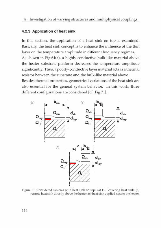
4 Investigation of varying structures and multiphysical couplings
4.2.3 Application of heat sink
In this section, the application of a heat sink on top is examined.Basically, the heat sink concept is to enhance the influence of the thinlayer on the temperature amplitude in different frequency regimes.As shown in Fig.64(a), a highly-conductive bulk-like material abovethe heater substrate platform decreases the temperature amplitudesignificantly. Thus, a poorly-conductive layer material acts as a thermalresistor between the substrate and the bulk-like material above.Besides thermal properties, geometrical variations of the heat sink arealso essential for the general system behavior. In this work, threedifferent configurations are considered [cf. Fig.71].
Ωs
ΩH
Ωlay dlay
Ωsin dsin
bsin(a)
Ωs
ΩH
Ωlay
Ωsin
dlay
dsin
bsin(b)
Ωs
ΩH
Ωlay
Ωsin
dlay
dsin
bsinc(c)
Figure 71: Considered systems with heat sink on top: (a) Full covering heat sink; (b)narrow heat sink directly above the heater; (c) heat sink applied next to the heater.
114

4 Investigation of varying structures and multiphysical couplings
0.00
0.50
1.00
1.50
2.00
2.50
3.00
101 102 103 104 105 106
∆T
[K]
Frequency fc [Hz]
Reference dlay=400nmdsin=50µmdsin=10µmdsin=5µmdsin=2µmdsin=1µm
(a)
0.00
0.50
1.00
1.50
2.00
2.50
3.00
3.50
101 102 103 104 105 106
∆T
[K]
Frequency fc [Hz]
Reference dlay=400nmdsin=50µmdsin=10µmdsin=5µmdsin=2µmdsin=1µm
(b)
Figure 72: Height variation for a full covering heat sink. A thin covering (a) STO and (b)PCMO layer is placed between the sink and the substrate. The system propertiesare: P/L = 5 W/m, Pt heater, a = 100 nm, 2b = 10 µm, dlay = 400 nm, Cu heatsink, ds = 1 mm, htc = 5 · 107 W/m2K.
The intention of different geometries is to increase the influence ofeither the cross- or in-plane thermal conductivity on the temperatureamplitude in different frequency regimes. First, a full coveringheat sink is examined for the anisotropic thermal conductivitydetermination. Here, a ‘full covering’ heat sink does not equalthe substrate width [Fig.13], because the voltage and current padsmust not be covered by the material on top of the heater structure.In the following systems, a full covering heat sink has a width of2bsin = 500 µm. Also the height of the heat sink is limited. Due tofabrication steps and the general feasibility, thin copper (Cu) foils aredesired as heat sink material. Therefore, we limit the height of the heatsink to dsin = 50 µm.Apparently, applying a heat sink on top changes the system behaviorfor an STO [cf. Fig.72(a)] and PCMO [cf. Fig.72(b)] layer significantly.Since the heat sink is placed on top of the structure, a misalignmentin positioning could occur. The influence on the ∆T -line is shown inFig.73.
115

4 Investigation of varying structures and multiphysical couplings
0.00
0.20
0.40
0.60
0.80
101 102 103 104 105 106
∆T
[K]
Frequency fc [Hz]
dsin=2µmdsin=2µm, shift of 150µm
Figure 73: Comparison of a 500 µm broad centrosymmetric aligned heat sink and heatsink with a 150 µm side shift. The system properties are: P/L = 5 W/m, Pt heater,a = 100 nm, 2b = 10 µm, PCMO layer, dlay = 400 nm, Cu heat sink, ds = 1 mm,htc = 5 · 107 W/m2K.
In relation to the tremendous shift of 150 µm to the side, the observeddifference is rather small. In case a slight misalignment is detectedafter positioning, higher measuring frequencies can counteract theshift.Obviously, the heat sink changes the ∆T -lines significantly. However,since the aim is to determine the anisotropic thermal conductivity ofthe layer, the question arises whether the sensitivity for the layer isenhanced. Therefore, the anisotropic variation is shown in Fig.74.Here, a full covering heat sink with a height of 2 µm is applied.In comparison to a pure applied layer on top [cf. Fig.70], the influenceof a poor cross-plane thermal conductivity is especially enhancedby this heat sink configuration. On the contrary, this system iscompletely insensitive for in-plane variations. Consequently, thisheat sink configuration is exclusively suitable for poorly-conductivecross-plane determinations.If the heat sink width is decreased, the system behaviour changestowards the behavior of thin films on top. However, the heat sinkmaterial is still present in the observed ∆T -line.
116
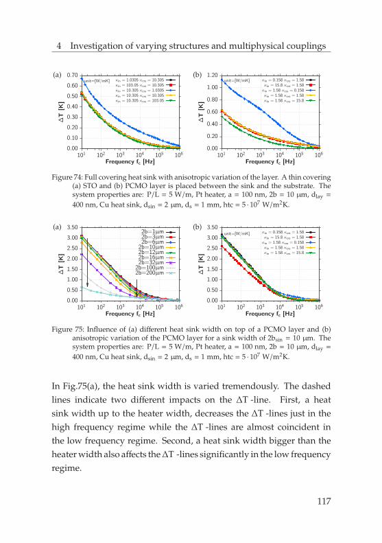
4 Investigation of varying structures and multiphysical couplings
0.00
0.10
0.20
0.30
0.40
0.50
0.60
0.70
101 102 103 104 105 106
∆T
[K]
Frequency fc [Hz]
unit=[W/mK] κin = 1.0305 κcrs = 10.305κin = 103.05 κcrs = 10.305κin = 10.305 κcrs = 1.0305κin = 10.305 κcrs = 10.305κin = 10.305 κcrs = 103.05
(a)
0.00
0.20
0.40
0.60
0.80
1.00
1.20
101 102 103 104 105 106
∆T
[K]
Frequency fc [Hz]
unit=[W/mK] κin = 0.158 κcrs = 1.58κin = 15.8 κcrs = 1.58κin = 1.58 κcrs = 0.158κin = 1.58 κcrs = 1.58κin = 1.58 κcrs = 15.8
(b)
Figure 74: Full covering heat sink with anisotropic variation of the layer. A thin covering(a) STO and (b) PCMO layer is placed between the sink and the substrate. Thesystem properties are: P/L = 5 W/m, Pt heater, a = 100 nm, 2b = 10 µm, dlay =
400 nm, Cu heat sink, dsin = 2 µm, ds = 1 mm, htc = 5 · 107 W/m2K.
0.00
0.50
1.00
1.50
2.00
2.50
3.00
3.50
101 102 103 104 105 106
∆T
[K]
Frequency fc [Hz]
2b=1µm2b=3µm2b=6µm
2b=10µm2b=12µm2b=16µm2b=32µm
2b=100µm2b=200µm
(a)
0.00
0.50
1.00
1.50
2.00
2.50
3.00
3.50
101 102 103 104 105 106
∆T
[K]
Frequency fc [Hz]
unit=[W/mK] κin = 0.158 κcrs = 1.58κin = 15.8 κcrs = 1.58κin = 1.58 κcrs = 0.158κin = 1.58 κcrs = 1.58κin = 1.58 κcrs = 15.8
(b)
Figure 75: Influence of (a) different heat sink width on top of a PCMO layer and (b)anisotropic variation of the PCMO layer for a sink width of 2bsin = 10 µm. Thesystem properties are: P/L = 5 W/m, Pt heater, a = 100 nm, 2b = 10 µm, dlay =
400 nm, Cu heat sink, dsin = 2 µm, ds = 1 mm, htc = 5 · 107 W/m2K.
In Fig.75(a), the heat sink width is varied tremendously. The dashedlines indicate two different impacts on the ∆T -line. First, a heatsink width up to the heater width, decreases the ∆T -lines just in thehigh frequency regime while the ∆T -lines are almost coincident inthe low frequency regime. Second, a heat sink width bigger than theheater width also affects the ∆T -lines significantly in the low frequencyregime.
117
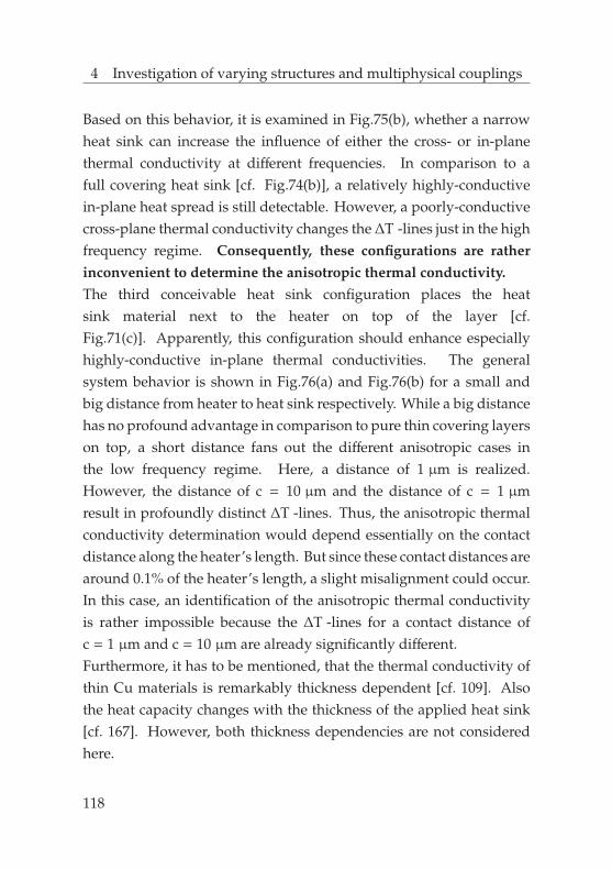
4 Investigation of varying structures and multiphysical couplings
Based on this behavior, it is examined in Fig.75(b), whether a narrowheat sink can increase the influence of either the cross- or in-planethermal conductivity at different frequencies. In comparison to afull covering heat sink [cf. Fig.74(b)], a relatively highly-conductivein-plane heat spread is still detectable. However, a poorly-conductivecross-plane thermal conductivity changes the ∆T -lines just in the highfrequency regime. Consequently, these configurations are ratherinconvenient to determine the anisotropic thermal conductivity.The third conceivable heat sink configuration places the heatsink material next to the heater on top of the layer [cf.Fig.71(c)]. Apparently, this configuration should enhance especiallyhighly-conductive in-plane thermal conductivities. The generalsystem behavior is shown in Fig.76(a) and Fig.76(b) for a small andbig distance from heater to heat sink respectively. While a big distancehas no profound advantage in comparison to pure thin covering layerson top, a short distance fans out the different anisotropic cases inthe low frequency regime. Here, a distance of 1 µm is realized.However, the distance of c = 10 µm and the distance of c = 1 µmresult in profoundly distinct ∆T -lines. Thus, the anisotropic thermalconductivity determination would depend essentially on the contactdistance along the heater’s length. But since these contact distances arearound 0.1% of the heater’s length, a slight misalignment could occur.In this case, an identification of the anisotropic thermal conductivityis rather impossible because the ∆T -lines for a contact distance ofc = 1 µm and c = 10 µm are already significantly different.Furthermore, it has to be mentioned, that the thermal conductivity ofthin Cu materials is remarkably thickness dependent [cf. 109]. Alsothe heat capacity changes with the thickness of the applied heat sink[cf. 167]. However, both thickness dependencies are not consideredhere.
118

4 Investigation of varying structures and multiphysical couplings
0.00
0.50
1.00
1.50
2.00
2.50
3.00
101 102 103 104 105 106
∆T
[K]
Frequency fc [Hz]
unit=[W/mK] κin = 0.158 κcrs = 1.58κin = 15.8 κcrs = 1.58κin = 1.58 κcrs = 0.158κin = 1.58 κcrs = 1.58κin = 1.58 κcrs = 15.8
(a)
0.00
0.50
1.00
1.50
2.00
2.50
101 102 103 104 105 106
∆T
[K]
Frequency fc [Hz]
unit=[W/mK]κin = 0.158 κcrs = 1.58κin = 15.8 κcrs = 1.58κin = 1.58 κcrs = 0.158κin = 1.58 κcrs = 1.58κin = 1.58 κcrs = 15.8
(b)
Figure 76: Influence of anisotropic variation for a (a) far placed heat sink with a distancec = 10 µm and a (b) near placed heat sink with a distance c = 1 µm. The heat sinkwidth on each side of the heater is 500 µm − 2b − c. The system properties are:P/L = 5 W/m, Pt heater, a = 100 nm, 2b = 10 µm, dlay = 400 nm, Cu heat sink,dsin = 2 µm, ds = 1 mm, htc = 5 · 107 W/m2K.
4.2.4 Patterned multilayer structures
Theoretically, it is also possible to place nanopatterned materials ontop of a heater substrate platform such as in Fig.77.
Ωs
ΩH
... Ωlay
dlay1
dlay2
Figure 77: Considered system for nanopatterns on top.
The sensitivity for various patterned PCMO and STO combinations ontop of a poorly- and highly-conductive substrate material is shown inFig.78. The resulting ∆T -lines are almost exclusively affected in thehigh frequency regime.
119

4 Investigation of varying structures and multiphysical couplings
0.00
0.05
0.10
0.15
101 102 103 104 105 106
∆T
[K]
Frequency fc [Hz]
Heater substrate referencedlay=100nmdlay=400nm
dlay=1000nm
(a)
0.00
0.05
0.10
0.15
101 102 103 104 105 106
∆T
[K]
Frequency fc [Hz]
Heater substrate referencedlay=100nmdlay=400nm
dlay=1000nm
(b)
0.00
0.05
0.10
0.15
101 102 103 104 105 106
∆T
[K]
Frequency fc [Hz]
Heater substrate referencePCMO-STO stack, 10 · 100nmSTO-PCMO stack, 10 · 100nm
(c)
0.00
1.00
2.00
3.00
4.00
101 102 103 104 105 106
∆T
[K]
Frequency fc [Hz]
Heater substrate referencePCMO-STO stack, 10 · 100nmSTO-PCMO stack, 10 · 100nm
(d)
Figure 78: Sensitivity of patterned materials. Influence of placing (a) PCMO, (b) STOmaterial on top of a MgO substrate. Fig.(c) and Fig.(d) show patterned multilayerstacks on a MgO and YSZ substrate respectively. Here, the width of the materialequals the heater’s width. The system properties are: P/L = 5 W/m, Pt heater,a = 100 nm, 2b = 10 µm, ds = 1 mm, htc = 5 · 107 W/m2K.
For significant changes, enormous stack heights would be requiredfor poorly-conductive thermoelectic materials. Moreover, these idealsystems are rather difficult to manufacture. However, if thesestructures could be manufactured, relatively high power per lengthwould be required in combination with measurements up to 1 MHz,in order to obtain temperature amplitude variations bigger than theerror in the experimental measurement.
120

4 Investigation of varying structures and multiphysical couplings
4.3 Membrane structures
Every previously investigated geometric structure contained abulk-like substrate geometry. While most of these geometryconfigurations are suitable to determine the cross-plane thermalconductivity, not every configuration is adequate to determine thein-plane thermal conductivity. Moreover, every configuration is almostinsensitive for poorly-conductive in-plane thermal conductivities.However, since we focus especially on poorly-conductive materials,a general configuration is required to also determine thepoorly-conductive in-plane case. Therefore, membrane structures areinvestigated in this section.First, two-dimensional membrane systems are considered to developan understanding of how temperature amplitude lines differ frombulk-like substrates. Here, only thermal simulations are examined.In the beginning, every outer boundary is considered to be adiabaticexpect the boundary to the substrate mount. This boundary takesinto account a htc. However, since the temperature amplitudes areexpected to be significantly higher than for bulk-like substrates withthe same applied power per length, radiation losses are also studied.Therefore, we apply the radiation boundary condition of Eq.4.6 at theouter boundaries of the membrane.Second, three-dimensional membrane systems are examined. Here, weconsider every boundary, except the substrate mount to be adiabatic.The substrate mount involves a htc. Moreover, we also consider themechanical field of Sec.3.1.3, to examine occurring displacements,deflections, and stresses. The thermal and mechanical boundaryconditions are given in Sec.3.
121
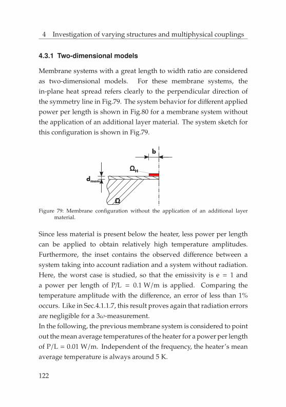
4 Investigation of varying structures and multiphysical couplings
4.3.1 Two-dimensional models
Membrane systems with a great length to width ratio are consideredas two-dimensional models. For these membrane systems, thein-plane heat spread refers clearly to the perpendicular direction ofthe symmetry line in Fig.79. The system behavior for different appliedpower per length is shown in Fig.80 for a membrane system withoutthe application of an additional layer material. The system sketch forthis configuration is shown in Fig.79.
Ω
b
dmem
ΩH
Figure 79: Membrane configuration without the application of an additional layermaterial.
Since less material is present below the heater, less power per lengthcan be applied to obtain relatively high temperature amplitudes.Furthermore, the inset contains the observed difference between asystem taking into account radiation and a system without radiation.Here, the worst case is studied, so that the emissivity is e = 1 anda power per length of P/L = 0.1 W/m is applied. Comparing thetemperature amplitude with the difference, an error of less than 1%occurs. Like in Sec.4.1.1.7, this result proves again that radiation errorsare negligible for a 3ω-measurement.In the following, the previous membrane system is considered to pointout the mean average temperatures of the heater for a power per lengthof P/L = 0.01 W/m. Independent of the frequency, the heater’s meanaverage temperature is always around 5 K.
122

4 Investigation of varying structures and multiphysical couplings
0.00
2.00
4.00
6.00
8.00
10.00
12.00
14.00
101 102 103 104 105 106
∆T
[K]
Frequency fc [Hz]
−2 · 10−1
0 · 100
101 106
∆T
ra−∆T P/L=0.001
P/L=0.003P/L=0.006P/L=0.01P/L=0.03P/L=0.06P/L=0.1
Figure 80: Comparison of different applied power per length P/L. The inset containsthe difference for a case with radiation at all outermost boundaries ∆T ra andwithout radiation ∆T for a P/L = 0.1 W/m. The system properties are: Pt heater,a = 100 nm, 2b = 10 µm, silicon nitride (SIN) membrane, 2bmem = 100 µm,dmem = 100 nm, silicon (Si) substrate, ds = 0.5 mm, htc = 5 · 107 W/m2K.
However, the maximum mean temperature is approximately 10 K fora frequency of fc = 10 Hz and approximately 5 K for a frequency offc = 1 MHz.To investigate thin layer materials, three distinct configurations exist ingeneral [cf. Fig.81]. The investigated material is either placed betweenthe heater and the membrane, placed on top of the heater membranesystem, or placed below the membrane.The general system behavior for different membrane widths is shownin Fig.82. According to Fig.81, three different layer applicationsare shown in comparison to a pure membrane system. Basically, abroad membrane implies a higher temperature amplitude. Thus weconclude, that small variations in the anisotropy change the ∆T signalmore significantly because the absolute values of ∆T are biggerthan for small membranes. In general, this does not depend on thedifferent layer application. Almost no difference occurs between thedifferent systems. In Fig.82, a poorly-conductive layer is applied. Theratio between the thermal conductivity of the layer material to themembrane material is κlay/κmem ≈ 0.66.
123

4 Investigation of varying structures and multiphysical couplings
Ω
b
dlaydmem
ΩH
(a)
Ω
b
dlaydmem
ΩH
(b)
Ω
b
dlaydmem
ΩH
(c)
Figure 81: (a) Investigated layer between heater and membrane; (b) layer placed ontop of heater membrane structure; (c) layer placed below the heater membranestructure.
A highly-conductive layer material with a bigger κlay/κmem ratioincreases the difference between the various layer applications slightly.After examining the general system behavior, different membranethicknesses are studied for the sensitivity to anisotropic thermalconduction. Since the membrane is only used for the purpose ofinvestigating the layer material, its desired thickness has to be as thinas possible. Furthermore, a non-conductive membrane would be idealto isolate the thermal properties of the layer material. Because in thiscase, the temperature amplitude would only depend on the thermalproperties of the layer to be investigated. However, the membranemust obviously exhibit thermal properties and a thickness.The sensitivity for a poorly- and moderately-conductive layer materialis examined in Fig.83. First, a comparison of Fig.83(a)83(c)83(e)and Fig.83(b)83(d)83(f) bares, that a thinner membrane increases thetemperature amplitude in general for both investigated materials.
124

4 Investigation of varying structures and multiphysical couplings
0.00
0.20
0.40
0.60
0.80
1.00
101 102 103 104 105 106
∆T
[K]
Frequency fc [Hz]
2bmem=10µm2bmem=20µm2bmem=50µm2bmem=100µm
(a)
0.00
0.10
0.20
0.30
0.40
0.50
101 102 103 104 105 106
∆T
[K]
Frequency fc [Hz]
2bmem=10µm2bmem=20µm2bmem=50µm2bmem=100µm
(b)
0.00
0.10
0.20
0.30
0.40
0.50
101 102 103 104 105 106
∆T
[K]
Frequency fc [Hz]
2bmem=10µm2bmem=20µm2bmem=50µm2bmem=100µm
(c)
0.00
0.10
0.20
0.30
0.40
0.50
101 102 103 104 105 106
∆T
[K]
Frequency fc [Hz]
2bmem=10µm2bmem=20µm2bmem=50µm2bmem=100µm
(d)
Figure 82: System behavior for two-dimensional membrane systems. (a) Pure membraneon substrate system, (b) layer between the heater and the membrane, (c) layerplaced on top of heater and membrane and (d) layer placed below the membrane.The system properties are: P/L = 0.01 W/m, Pt heater, a = 100 nm, 2b = 10 µm,PCMO layer, dlay = 400 nm, SIN membrane, dmem = 100 nm, Si substrate, ds =
0.5 mm, htc = 5 · 107 W/m2K.
Second, these membrane systems are almost exclusively sensitiveto anisotropic in-plane thermal conductivity variations. Cross-planevariations do not affect the temperature amplitudes. Moreover,differences in ∆T occur only in the low frequency regime.Consequently, the dimensions of the membrane limit essentially thesensitivity for the in-plane conduction. However, we conclude thatmembrane configurations which are fabricated via micro electromechanical systems (MEMS), with a bigger membrane width than2b ≥ 100 µm and a thickness less than dmem ≤ 100 nm are suitableto determine the in-plane thermal conductivity for both materialsPCMO and STO.
125

4 Investigation of varying structures and multiphysical couplings
0.00
0.10
0.20
0.30
0.40
0.50
101 102 103 104 105 106
∆T
[K]
Frequency fc [Hz]
unit=[W/mK]κin = 0.158 κcrs = 1.58κin = 15.8 κcrs = 1.58κin = 1.58 κcrs = 0.158κin = 1.58 κcrs = 1.58κin = 1.58 κcrs = 15.8
(a)
0.00
0.10
0.20
0.30
0.40
0.50
101 102 103 104 105 106
∆T
[K]
Frequency fc [Hz]
unit=[W/mK] κin = 1.0305 κcrs = 10.305κin = 103.05 κcrs = 10.305κin = 10.305 κcrs = 1.0305κin = 10.305 κcrs = 10.305κin = 10.305 κcrs = 103.05
(b)
0.00
0.25
0.50
0.75
1.00
101 102 103 104 105 106
∆T
[K]
Frequency fc [Hz]
unit=[W/mK]
κin = 0.158 κcrs = 1.58κin = 15.8 κcrs = 1.58κin = 1.58 κcrs = 0.158κin = 1.58 κcrs = 1.58κin = 1.58 κcrs = 15.8
(c)
0.00
0.10
0.20
0.30
0.40
0.50
101 102 103 104 105 106
∆T
[K]
Frequency fc [Hz]
unit=[W/mK] κin = 1.0305 κcrs = 10.305κin = 103.05 κcrs = 10.305κin = 10.305 κcrs = 1.0305κin = 10.305 κcrs = 10.305κin = 10.305 κcrs = 103.05
(d)
0.00
0.50
1.00
1.50
2.00
101 102 103 104 105 106
∆T
[K]
Frequency fc [Hz]
unit=[W/mK] κin = 0.158 κcrs = 1.58κin = 15.8 κcrs = 1.58κin = 1.58 κcrs = 0.158κin = 1.58 κcrs = 1.58κin = 1.58 κcrs = 15.8
(e)
0.00
0.10
0.20
0.30
0.40
0.50
101 102 103 104 105 106
∆T
[K]
Frequency fc [Hz]
unit=[W/mK] κin = 1.0305 κcrs = 10.305κin = 103.05 κcrs = 10.305κin = 10.305 κcrs = 1.0305κin = 10.305 κcrs = 10.305κin = 10.305 κcrs = 103.05
(f)
Figure 83: Influence of membrane thickness for anisotropic layer material. Sensitivityfor an anisotropic PCMO layer material with a membrane thickness of (a) 200 nm,(c) 100 nm and (e) 30 nm. Sensitivity for an anisotropic STO layer material fora membrane thickness of (b) 200 nm, (d) 100 nm and (f) 30 nm. The systemproperties are: P/L = 0.01 W/m, Pt heater, a = 100 nm, 2b = 10 µm, PCMOlayer, dlay = 400 nm, SIN membrane, 2bmem = 100 µm, Si substrate, ds = 0.5 mm,htc = 5 · 107 W/m2K.
126

4 Investigation of varying structures and multiphysical couplings
4.3.2 Three-dimensional 6-pad heater structure
In the previous section, it is shown, that two-dimensional membranestructures are suitable to determine the in-plane thermal conductivity.However, these models ignore the heat conduction along the heater’slength dimension. But towards the end of the heater’s length, thusbehind the membrane area, a bulk-like substrate is present. Here,we apply a Si substrate. Si is regarded as a highly-conductivesubstrate material. As shown in Sec.4.1.2.1, highly-conductivesubstrates are especially appropriate to determine the cross-planethermal conductivity. Thus the question arises, whether a heaterstructure could combine these properties. Hence it is examined in thissection, whether a three-dimensional designed geometric structure hasthe potential to determine the cross- and in-plane thermal conductivitywith one geometry configuration. Moreover, we propose in this worka special heater configuration with six contact pads. The investigatedlayer material is placed between the heater and the membrane [cf.Fig.81(a)]. The general system sketch is shown in Fig.84.38
We call this configuration a 6-pad heater structure. The idea of the6-pad structure is to have two different measuring configurations.The first configuration is the so-called short heater configuration [cf.Fig.84(b)]. The current is applied through the middle pads (shaded inred) and the voltage is measured at the inner pads (shaded in green).We think that in this configuration, the voltage signal and thus thetemperature amplitude is dominated by the influence of the in-planethermal conductivity. The second configuration is the so-called longheater configuration [cf. Fig.84(c)].
38A technical drawing of the 6-pad structure is given in App.C.
127

4 Investigation of varying structures and multiphysical couplings
(a)
(b) (c)
Figure 84: (a) General system sketch for a 6-pad heater structure; (b) short heaterconfiguration; (c) long heater configuration. The applied heating is marked inred, the green color indicates the voltage tapping.
Here, the current is applied through the outer pads and the voltage ismeasured at the middle pads. In this configuration, the voltage signaland thus the temperature amplitude should also contain significantlythe influence of the cross-plane thermal conductivity. However, inboth configurations, only four pads are used for each measurement. Amain advantage of such a configuration would be the determinationof the cross- and in-plane thermal conductivity for one fabricatedsample and thus for persisting layer properties. The general systembehavior for the 6-pad structure is shown in Fig.85.First, the STO layer material is considered. In general, both heaterconfigurations [cf. Fig.85(a) and Fig.85(b)] exhibit a similar systembehavior in comparison to the two-dimensional model of membranesystems. It turns out that, the sensitivity for in-plane conduction is
128

4 Investigation of varying structures and multiphysical couplings
0.00
0.10
0.20
0.30
0.40
0.50
0.60
101 102 103 104 105 106
∆T
[K]
Frequency fc [Hz]
unit=[W/mK] κin = 1.0305 κcrs = 10.305κin = 103.05 κcrs = 10.305κin = 10.305 κcrs = 1.0305κin = 10.305 κcrs = 10.305κin = 10.305 κcrs = 103.05
(a)
0.00
0.05
0.10
0.15
0.20
0.25
0.30
101 102 103 104 105 106
∆T
[K]
Frequency fc [Hz]
unit=[W/mK] κin = 1.0305 κcrs = 10.305κin = 103.05 κcrs = 10.305κin = 10.305 κcrs = 1.0305κin = 10.305 κcrs = 10.305κin = 10.305 κcrs = 103.05
(b)
0.00
0.25
0.50
0.75
1.00
1.25
101 102 103 104 105 106
∆T
[K]
Frequency fc [Hz]
unit=[W/mK] κin = 0.158 κcrs = 1.58κin = 15.8 κcrs = 1.58κin = 1.58 κcrs = 0.158κin = 1.58 κcrs = 1.58κin = 1.58 κcrs = 15.8
(c)
0.00
0.10
0.20
0.30
0.40
0.50
0.60
101 102 103 104 105 106
∆T
[K]
Frequency fc [Hz]
unit=[W/mK] κin = 0.158 κcrs = 1.58κin = 15.8 κcrs = 1.58κin = 1.58 κcrs = 0.158κin = 1.58 κcrs = 1.58κin = 1.58 κcrs = 15.8
(d)
Figure 85: System behavior for a three-dimensional membrane system. Short heaterconfiguration for a (a) STO and (c) PCMO layer. Long heater configuration fora (b) STO and (d) PCMO layer. The system properties are: P/L = 0.05 W/m,Pt heater, a = 100 nm, 2b = 10 µm, PCMO layer, dlay = 500 nm, SIN membrane,dmem = 100 nm, 2bmem = 250 µm, Si substrate, ds = 0.5 mm, htc = 5 · 107 W/m2K.
higher for the short heater configuration, than for the long heaterconfiguration. Moreover, a comparison of the long and short heaterconfiguration exhibits, that the temperature amplitude in the longheater configuration is smaller than in the short heater configuration.This is because more thermal mass is present below the long heater.Second, the PCMO layer material is considered. Also here, the∆T -lines for a short heater configuration are similar to the ∆T -linesof the two-dimensional model of membrane systems.
129

4 Investigation of varying structures and multiphysical couplings
0.00
0.03
0.06
0.09
0.12
0.15
0.18
0.21
101 102 103 104 105 106
∆T
[K]
Frequency fc [Hz]
unit=[W/mK]
κin = 0.158 κcrs = 1.58κin = 15.8 κcrs = 1.58κin = 1.58 κcrs = 0.158κin = 1.58 κcrs = 1.58κin = 1.58 κcrs = 15.8
(a)
0.00
0.02
0.04
0.06
0.08
0.10
101 102 103 104 105 106
∆T
[K]
Frequency fc [Hz]
unit=[W/mK]
κin = 0.158 κcrs = 1.58κin = 15.8 κcrs = 1.58κin = 1.58 κcrs = 0.158κin = 1.58 κcrs = 1.58κin = 1.58 κcrs = 15.8
(b)
Figure 86: System behavior for a three-dimensional membrane system. The resultingtemperature amplitudes are shown in (a) for the short heater configuration and in(b) for the long heater configuration. The system properties are: P/L = 0.05 W/m,Pt heater, a = 100 nm, 2b = 10 µm, PCMO layer, cplay
= 48 J/kgK, dlay = 500 nm,SIN membrane, κmem = 30.1 W/mK, dmem = 100 nm, 2bmem = 250 µm, Sisubstrate, ds = 0.5 mm, htc = 5 · 107 W/m2K.
However, for both materials the long heater configuration is notsuitable to determine also the cross-plane thermal conductivity.Consequently, the proposed 6-pad heater structure can be applied todetermine the in-plane thermal conductivity for both materials STOand PCMO. But, it is not possible to determine the in- and cross-planethermal conductivity of the STO and PCMO layer simultaneously.However, in this work, we use a poorly-conductive SIN membrane.But in literature, also moderatley-conductive SIN membranes arereported with a thermal conductivity ofκmem = 30.1 W/mK [46]. Basedon such an SIN membrane material, we investigate further, if it wouldbe possible to determine the cross- and in-plane thermal conductivitywith the 6-pad structure. Moreover, for this investigation, we apply aPCMO like layer material where the heat capacity is decreased bya factor of ten so that cp = 48 J/kgK. The resulting temperatureamplitudes are shown in Fig.86. While the system behavior for theshort heater configuration is similar to Fig.85(c), the system behavior
130

4 Investigation of varying structures and multiphysical couplings
(a)
(b) (c)
Figure 87: (a) Illustration of the coordinate system, (b) the horizontal cut and (c) the cutalong the heater. The point of origin (0,0,0) is defined between the heater and thelayer material.
for the long heater configuration exhibits a distinctly different ∆T -linefor the extremely poorly-conductive cross-plane case [cf. Fig.86(b)].Here, the ∆T -line shifts up over the whole frequency regime.Thus essentially, the cross- and in-plane thermal conductivity of suchan extremely poorly-conductive layer material could be determinedby the proposed 6-pad heater structure with a moderately-conductiveSIN membrane.39 Here, the same power per length is applied than forthe poorly-conductive membrane so that Fig.86 is comparable to Fig.85.However, since the membrane’s thermal conductivity is higher here,the temperature amplitudes in Fig.86 are rather small. By applyinga power per length around P/L = 0.1 W/m, temperature amplitudesup to one Kelvin can be achieved, but essentially, the system behaviorremains the same.
39If the heat capacity of the layer is cp = 480 J/kgK, the blue ∆T -line in Fig.86 woulddecrease slightly in the high frequency regime, but the ∆T -line still differs significantlyfrom the other anisotropic cases.
131

4 Investigation of varying structures and multiphysical couplings
300.00
300.10
300.20
300.30
300.40
300.50
0 · 100 42 · 10−6 83 · 10−6 125 · 10−6
T[K
]
x [m]
fc=10 [Hz]Time point 1
2345
(a)
300.00
300.10
300.20
300.30
0 · 100 42 · 10−6 83 · 10−6 125 · 10−6
T[K
]
x [m]
fc=1000 [Hz]
Time point 12345
(b)
300.00
300.10
300.20
300.30
300.40
300.50
0 · 100 42 · 10−6 83 · 10−6 125 · 10−6
T[K
]
z [m]
fc=10 [Hz]Time point 1
2345
(c)
300.00
300.10
300.20
300.30
0 · 100 42 · 10−6 83 · 10−6 125 · 10−6
T[K
]
z [m]
fc=1000 [Hz]
Time point 12345
(d)
Figure 88: Temperature distribution along a (a),(b) horizontal and (c),(d) length cut.The cutting lines are located in the center of the layer. The system propertiesare: P/L = 0.05 W/m, Pt heater, 2b = 10 µm, a = 100 nm, dlay = 500 nm, STOlayer material, 2bmem = 250 µm, SIN membrane, Si substrate, ds = 0.5 mm andhtc = 5 · 107 W/m2K.
In the following, the spatial temperature distribution is examined forthe STO layer material to understand the system behavior. Accordingto Sec.4.1.1.4, five different time points are considered. In contrast totwo-dimensional model systems, one cut is regarded from the centerpoint of the heater towards the perpendicular side of the membrane.The other cut is along the heater towards the support of the substrate.Both cuts are situated in the center of the layer material. Fig.87illustrates these two cuts. The temperature distribution is shown inFig.88 for these two cuts.
132

4 Investigation of varying structures and multiphysical couplings
Here, Fig.88(a) and 88(c) show clearly decreasing temperature trendsfor each time point without an overlap. On the contrary, thetemperature lines in Fig.88(b) and 88(d) cross each other at a certainspatial length. For these systems, the spatial temperature distributiondoes not decrease as fast as for bulk-like materials. The reason is that,less material is present below the heat source.The cut along the heater’s length dimension exhibits a completelydifferent temperature distribution. Independent from the frequency,the spatial temperature amplitude decreases significantly towards thesubstrate support. This behavior indicates a high sensitivity for thein-plane thermal conduction and a relatively low sensitivity for thecross-plane conduction above the substrate support. This is because,the temperature amplitudes are in general tremendously smaller thanin the area of the membrane. The overall temperature distributionis shown in Fig.93 for the short heater configuration. Since a MEMSapplies a membrane with a big width to thickness ratio, the deflectionand occurring stresses within a measurement are investigated in thefollowing. According to results, the maximum deflection occurs at thecenter of the membrane. Therefore, we observe the displacement ofa single point located between the heater and the membrane. Fig.89illustrates the considered point for a short heater configuration.
Figure 89: Illustration of the considered point of deflection at (0,0,0) for the short heaterconfiguration.
133

4 Investigation of varying structures and multiphysical couplings
0.00 · 100
2.50 · 10−10
5.00 · 10−10
7.50 · 10−10
1.00 · 10−9
1.25 · 10−9
3.02 3.04 3.06 3.08
uy[m
]
Time [s]
(a)
4.930 · 10−10
4.933 · 10−10
4.935 · 10−10
4.938 · 10−10
4.940 · 10−10
0.0000302 0.0000304 0.0000306 0.0000308
uy[m
]
Time [s]
(b)
0.00 · 100
1.25 · 10−9
2.50 · 10−9
3.75 · 10−9
5.00 · 10−9
3.02 3.04 3.06 3.08
uy[m
]
Time [s]
(c)
2.489 · 10−9
2.490 · 10−9
2.491 · 10−9
2.493 · 10−9
0.0000302 0.0000304 0.0000306 0.0000308
uy[m
]
Time [s]
(d)
Figure 90: Deflection of the center point for a three-dimensional membrane systemwith the short heater configuration. Deflection for a STO and PCMO layer at(a)(c) 10 Hz and (b)(d) 1 MHz respectively. The system properties are: P/L =0.05 W/m, Pt heater, a = 100 nm, 2b = 10 µm, dlay = 500 nm, SIN membrane,dmem = 100 nm, 2bmem = 250 µm, Si substrate, ds = 0.5 mm, htc = 5 · 107 W/m2K.
The deflections of the center point are shown in Fig.90. The deflectionnecessarily follows the temperature behavior in general for bothinvestigated materials. While the deflection returns almost to zerofor a frequency of fc = 10 Hz, the displacement remains at a higherdeflection for a frequency of fc = 1 MHz. However, for bothinvestigated materials, the deflections of the center point are certainlyless than 10 nm. Moreover, the maximum displacements of the otherspatial dimensions are even smaller [cf. Fig.93].
134
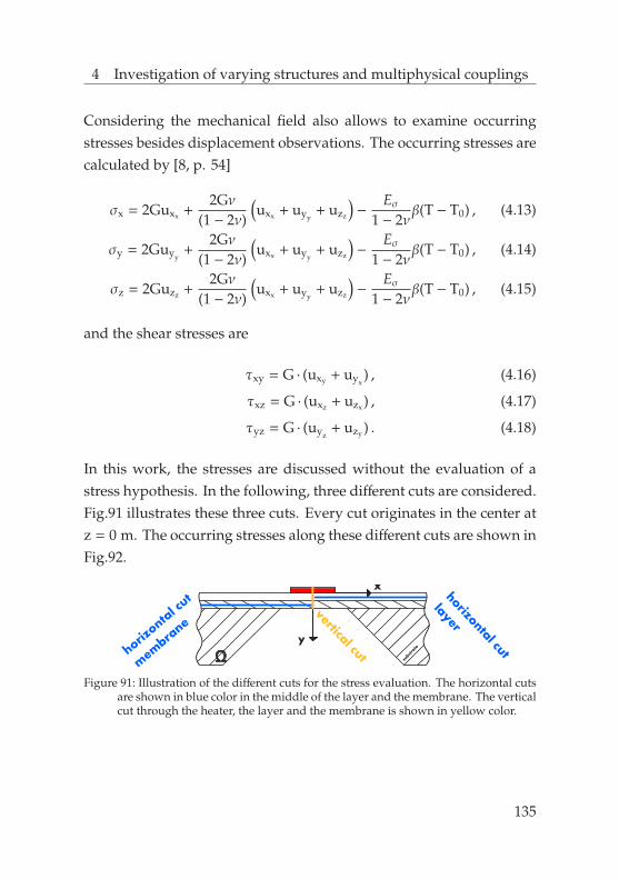
4 Investigation of varying structures and multiphysical couplings
Considering the mechanical field also allows to examine occurringstresses besides displacement observations. The occurring stresses arecalculated by [8, p. 54]
σx = 2Guxx +2Gν
(1 − 2ν)
(uxx + uyy
+ uzz
)−
Eσ1 − 2ν
β(T − T0) , (4.13)
σy = 2Guyy+
2Gν(1 − 2ν)
(uxx + uyy
+ uzz
)−
Eσ1 − 2ν
β(T − T0) , (4.14)
σz = 2Guzz +2Gν
(1 − 2ν)
(uxx + uyy
+ uzz
)−
Eσ1 − 2ν
β(T − T0) , (4.15)
and the shear stresses are
τxy = G · (uxy + uyx) , (4.16)
τxz = G · (uxz + uzx ) , (4.17)
τyz = G · (uyz+ uzy ) . (4.18)
In this work, the stresses are discussed without the evaluation of astress hypothesis. In the following, three different cuts are considered.Fig.91 illustrates these three cuts. Every cut originates in the center atz = 0 m. The occurring stresses along these different cuts are shown inFig.92.
Ω subst
rate
x
y
vertical cuthorizonta
l cut
mem
brane
horizontal cut
layer
Figure 91: Illustration of the different cuts for the stress evaluation. The horizontal cutsare shown in blue color in the middle of the layer and the membrane. The verticalcut through the heater, the layer and the membrane is shown in yellow color.
135

4 Investigation of varying structures and multiphysical couplings
-1
0
1
σ[N
/m
2]
layer
-1
0
1
0 35 70 105 140
σ[N
/m
2]
x [µm]
membrane
σxσyσz
τxzτxyτyz
(a)
-1
-0.5
0
0.5
1
-100 0 100 200 300 400 500 600
σ[N
/m
2]
y [nm]
σxσyσzτxzτxyτyz
(b)
Figure 92: Occurring stress for a cut (a) horizontal from the center point in the middle ofthe layer and in the middle of the membrane towards the membrane’s side and(b) a vertical cut over the height at the center point. The system properties are:P/L = 0.05 W/m, Pt heater, a = 100 nm, 2b = 10 µm, STO layer, dlay = 500 nm,SIN membrane, dmem = 100 µm, 2bmem = 250 µm, Si substrate, ds = 0.5 mm,htc = 5 · 107 W/m2K.
While Fig.92(a) shows the occurring spatial stresses along a horizontalcut line in the middle of the layer and the middle of the membrane,Fig.92(b) shows the occurring spatial stresses over the thickness ofthe heater layer and membrane package. First, the horizontal cutis considered. The first inset of Fig.92(a) shows the stresses in themiddle of the layer. All stresses are almost zero, except the stressesσx and σz. The layer is under pressure until the substrate mount. Onthe contrary, the second inset of Fig.92(a) shows that the membraneis under tension for approximately a quarter of the total membranewidth. All magnitudes decrease significantly towards the substratesupport. Second, the vertical cut is regarded. Fig.92(b) shows thestresses along this cut. All stresses are almost zero, except the stressesσx and σz. Here, these two stresses differ slightly from each materialto the neighboring material. While the heater and the layer are underpressure, the membrane exhibits almost no stress. However, in generalall occurring stress magnitudes are extremely small and we don’texpect any material to fail with this small applied power per length.
136
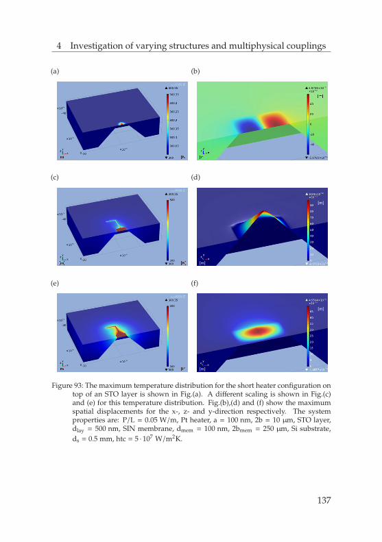
4 Investigation of varying structures and multiphysical couplings
(a) (b)
(c)
[m]
[m]
(d)
(e)
[m]
[m]
(f)
Figure 93: The maximum temperature distribution for the short heater configuration ontop of an STO layer is shown in Fig.(a). A different scaling is shown in Fig.(c)and (e) for this temperature distribution. Fig.(b),(d) and (f) show the maximumspatial displacements for the x-, z- and y-direction respectively. The systemproperties are: P/L = 0.05 W/m, Pt heater, a = 100 nm, 2b = 10 µm, STO layer,dlay = 500 nm, SIN membrane, dmem = 100 nm, 2bmem = 250 µm, Si substrate,ds = 0.5 mm, htc = 5 · 107 W/m2K.
137

4 Investigation of varying structures and multiphysical couplings
4.4 Pillar and pad structure
Contrary to a 3ω-measurement, the pillar and pad experiments applythe PCMO material itself as a heating material. The three-dimensionalstructure, the system definitions and the pillar’s and pad’s dimensionsare shown in Fig.94.
(a) (b)
(c) (d)
Figure 94: Scanning electron microscopy (SEM) images of the (a) three-dimensional pillarstructure and (b) the PCMO pad structure with an electrically insulating PMMAlayer. The SEM images were taken by our project partners at the University ofGottingen. The corresponding system definitions and dimensions are given in (c)for the pillar and in (d) for the pad structure.
138

4 Investigation of varying structures and multiphysical couplings
In the beginning, the PCMO pillar is considered [cf. Fig.94(c)]. Here,we distinguish between two different configurations. First, a pillarwhere only a small Pt electrode is placed on top of the PCMO material.Second, a pillar where a tungsten (W) needle (Kleindiek) is in thermalcontact with the Pt top electrode.40
Afterwards, the PCMO pad device is considered [cf. Fig.94(d)].Here, a PCMO layer is placed between a Pt top and bottomelectrode. This sandwiched structure encloses an electrically insulatingPolymethyl Methacrylate (PMMA) layer (C5H8O2) to realize a pillarlike PCMO structure.41 Although, the Pt materials above and belowthe PCMO material exist to induce the current, both the pillar andpad investigations, apply Joule heating only in the area of thePCMO material, because the electric resistivity of Pt is negligible incomparison to PCMO.In contrast to the previous investigations for 3ω-measurements, thepillars exhibit a rotation symmetry which we use for the simulationsto reduce computing time. The respective governing equations aregiven in Sec.3.1.1. Here, the power input is not regarded as a powerper length and not applied with an angular frequency. According toSec.3.1.1, the heat source term of Eq.3.16 writes now to
p = %0(T) · j(t)2 . (4.19)
Here, %0(T) is the temperature dependent specific electric resistivityand j(t) is the current density. Details about the application of the timedependent current density are given in Sec.3.2.
40Find App.B for further information about W.41Find App.B for further information about PMMA.
139

4 Investigation of varying structures and multiphysical couplings
0
10000
20000
30000
40000
50000
60000
140 160 180 200 220 240 260 280 300
R[Ω]
Temperature[K]
Measured resistanceFit function
(a)
0
10000
20000
30000
40000
50000
60000
200 300 400 500 600 700 800 9001000
R[Ω]
Temperature[K]
280
380
480
280 290 300
Measured resistanceFit function
(b)
Figure 95: (a)(b) Experimentally measured data points of the electric resistance andcorresponding fit function for the PCMO pillar of Fig.94(a) with a radius of rp =3 µm and a height of dPCMO = 300 nm.
The specific electric resistivity is calculated by
%0(T) =R(T) ·Ap
dPCMO. (4.20)
Here, Ap = π · r2p is the circular surface area of the pillar with the
radius rp and R(T) is the electric resistance behavior, which wasexperimentally measured. Moreover, the electric resistance behavioris strongly non-linear with temperature. The temperature dependentresistivity is shown in Fig.95. Experimental data points are just existentuntil 300 K.However, since current densities are applied up to j = 1 · 1010 A/m2, weexpect a tremendous temperature increase. In this work, a fit functionis used. Thus, the known experimental data is represented and theelectric resistance behavior is further extrapolated. The fit functiondecreases strictly monotonically up to several thousand Kelvin, butalways remains positive. The fit function writes to
R(T) = 77.86/√
T · e1272.26/T [Ω] . (4.21)
140

4 Investigation of varying structures and multiphysical couplings
Although we do not know the melting point of PCMO, we knowthat it must be over 1300 K since its thermoelectric properties arecharacterized up to this temperature [cf. 43]. According to Sec.3.1.1,we assume that no heat flows through the axis of symmetry Γ1 andthe outer boundaries Γ2 and Γ3. In contrast to the 3ω-simulations, thesubstrate mount is considered isothermal so that
Γ4 : T = T0 . (4.22)
In the following, three different initial and ambient temperatures arestudied
Ω : Tinit = T0 = 300, 230, 160 K . (4.23)
Since the heat capacity of PCMO changes especially for lowtemperatures [cf. 102], a linear function is used in this section for theheat capacity of PCMO. This funtion writes to
cp =
0 ≤ T ≤ 230 : 2.087 ·T [J/kgK]
230 < T < ∞ : 480 [J/kgK] .(4.24)
The resulting time dependent temperature behavior for the pillarwithout the Kleindiek contact is shown in Fig.96. Here the temperaturerepresents the mean temperature in the PCMO material, determinedby Eq.3.17.
141

4 Investigation of varying structures and multiphysical couplings
0
200
400
600
800
1000
1200
1400
10−3 10−2 10−1 100 101 102
Tmea
n[K
]
t [s]
unit=[A/m2] j=1 · 107j=1 · 108j=1 · 109j=5 · 109j=1 · 1010
(a)
0
200
400
600
800
1000
1200
1400
0.0030015 0.0030025 0.0030035
Tmea
n[K
]
t [s]
unit=[A/m2] j=1 · 107j=1 · 108j=1 · 109j=5 · 109j=1 · 1010
(b)
0
200
400
600
800
1000
1200
1400
10−3 10−2 10−1 100 101 102
Tmea
n[K
]
t [s]
unit=[A/m2] j=1 · 107j=1 · 108j=1 · 109j=5 · 109j=1 · 1010
(c)
0
200
400
600
800
1000
1200
1400
0.0030015 0.0030025 0.0030035
Tmea
n[K
]
t [s]
unit=[A/m2] j=1 · 107j=1 · 108j=1 · 109j=5 · 109j=1 · 1010
(d)
Figure 96: The pillar’s time dependent mean temperature behavior for an initialtemperature of 300 K for (a) durp = 1 s and (b) durp = 1 µs and for an initialtemperature of 160 K for (c) durp = 1 s and (d) durp = 1 µs.
Fig.96 is discussed in the following. First, independent of the initialtemperature and pulse length, a current density of j = 1 · 1010 A/m2
results in the maximum temperature increase. Second, alreadycurrent densities which are applied for 1 µs result in remarkably hightemperatures in comparison to current densities which are applied for1 s. Thus, the major part of heating takes place in the first micro second.Third, for every initial temperature and simulated current density, thetemperature returns back to initial condition within the pulse repetitionrate fp, although temperatures up to 1200 K occur. This fact is shownin Fig.97 for a reference current density of j = 1 · 1010 A/m2.
142
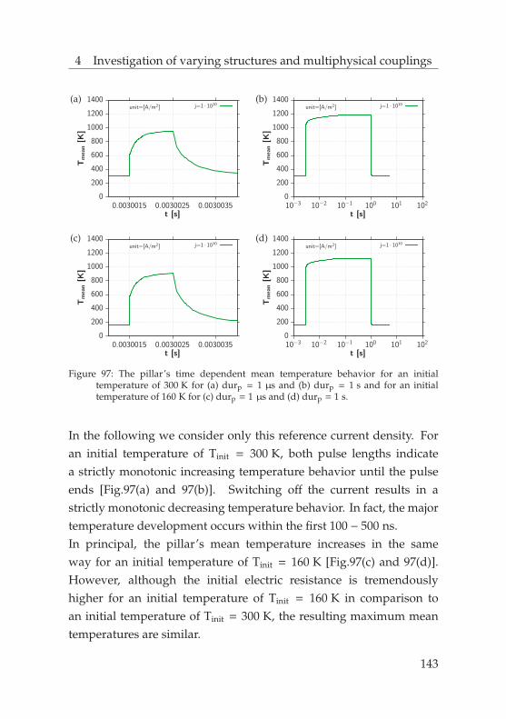
4 Investigation of varying structures and multiphysical couplings
0
200
400
600
800
1000
1200
1400
0.0030015 0.0030025 0.0030035
Tmea
n[K
]
t [s]
unit=[A/m2] j=1 · 1010(a)
0
200
400
600
800
1000
1200
1400
10−3 10−2 10−1 100 101 102
Tmea
n[K
]
t [s]
unit=[A/m2] j=1 · 1010(b)
0
200
400
600
800
1000
1200
1400
0.0030015 0.0030025 0.0030035
Tmea
n[K
]
t [s]
unit=[A/m2] j=1 · 1010(c)
0
200
400
600
800
1000
1200
1400
10−3 10−2 10−1 100 101 102
Tmea
n[K
]
t [s]
unit=[A/m2] j=1 · 1010(d)
Figure 97: The pillar’s time dependent mean temperature behavior for an initialtemperature of 300 K for (a) durp = 1 µs and (b) durp = 1 s and for an initialtemperature of 160 K for (c) durp = 1 µs and (d) durp = 1 s.
In the following we consider only this reference current density. Foran initial temperature of Tinit = 300 K, both pulse lengths indicatea strictly monotonic increasing temperature behavior until the pulseends [Fig.97(a) and 97(b)]. Switching off the current results in astrictly monotonic decreasing temperature behavior. In fact, the majortemperature development occurs within the first 100 − 500 ns.In principal, the pillar’s mean temperature increases in the sameway for an initial temperature of Tinit = 160 K [Fig.97(c) and 97(d)].However, although the initial electric resistance is tremendouslyhigher for an initial temperature of Tinit = 160 K in comparison toan initial temperature of Tinit = 300 K, the resulting maximum meantemperatures are similar.
143

4 Investigation of varying structures and multiphysical couplings
vertical cut
horizontal cut = hc1
hc2
hc3
Figure 98: Definition of a vertical cut (yellow) and three horizontal cuts (blue) within thepillar configuration.
To understand the different temperature developments, vertical andhorizontal cuts through the pillars are taken into consideration in thefollowing. The cuts are defined in Fig.98. First, the pillar withoutthe Kleindiek contact is considered and the horizontal cut hc1 and thevertical cut are examined. Subsequently, the pad device is examinedwith two additional horizontal cuts, hc2 and hc3.Fig.99 shows the temperature profiles for an initial temperatureof Tinit = 300 K at several time steps within the heating pulse.Since basically, both pulse durations exhibit the same temperaturedevelopment along the vertical cut and the horizontal cut hc1 for thefirst 1 µs, we consider only a pulse duration of 1 s in the following.However, higher temperatures occur for a pulse duration of 1 s.The time intervals for a vertical cut indicate a rapid temperatureincrease in the center of the PCMO layer [cf. Fig.99(a)]. Since it requiressome time for heat to diffuse into the top Pt electrode, a time lag ofthe respective local maximum temperature is visible. Despite this lag,the temperature in the top electrode adapts to the temperature of thePCMO layer before the pulse is completed. In case of the free standingpillar, the maximum temperature occurs at the top of the PCMO layer.The temperature below the PCMO layer increases significantly slowersince heat is conducted into the substrate.
144

4 Investigation of varying structures and multiphysical couplings
0
200
400
600
800
1000
1200
1400
1600
1800
0.0 · 100 5.0 · 10−7 1.0 · 10−6 1.5 · 10−6
T[K
]
distance [m]
t=0.0030015000001st=0.0030015001st=0.0030015005st=0.003001505st=0.00300152st=0.0030016st=0.0030025s
t=1.0s
(a)
0200400600800100012001400160018002000
0.0 · 100 1.0 · 10−6 2.0 · 10−6
T[K
]
distance [m]
t=0.0030015000001st=0.0030015001st=0.0030015005st=0.003001505st=0.00300152st=0.0030016st=0.0030025s
t=1.0s
(b)
Figure 99: Temperature profiles for the pillar of Fig.94(c) without the Kleindiek contactand an initial temperature of Tinit = 300 K and a pulse duration of durp = 1 s.The vertical cut of 98 is shown in (a) and the horizontal cut hc1 is shown in(b). The temperature profiles are simulated for the reference current density ofj = 1 · 1010 A/m2.
Figure 100: Indicated area below the temperature profile to illustrate the averagetemperature along the vertical cut for comparison to the determined integraltemperature in the PCMO layer.
Moreover, the horizontal cut indicates that the maximum temperatureis always at the axis of symmetry and decreases towards the outerside of the pillar [cf. Fig.99(b)]. Due to this fact, the determinedmean temperature of the PCMO layer can be correlated to the averagetemperature along the vertical cut because the temperature gradientis almost zero, so that ∂T/∂r ≈ 0. This circumstance is illustrated inFig.100. Regarding this circumstance, several time points in Fig.99(a)illustrate the strictly monotonic temperature increase of Fig.97(a) and97(b). Thus, the mean PCMO temperature must increase until thepulse is completed because every increased time step results in highertemperatures.
145
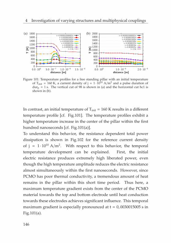
4 Investigation of varying structures and multiphysical couplings
0
200
400
600
800
1000
1200
1400
1600
1800
0.0 · 100 5.0 · 10−7 1.0 · 10−6 1.5 · 10−6
T[K
]
distance [m]
t=0.0030015000001st=0.0030015001st=0.0030015005st=0.003001505st=0.00300152st=0.0030016st=0.0030025s
t=1.0s
(a)
0200400600800100012001400160018002000
0.0 · 100 1.0 · 10−6 2.0 · 10−6
T[K
]
distance [m]
t=0.0030015000001st=0.0030015001st=0.0030015005st=0.003001505st=0.00300152st=0.0030016st=0.0030025s
t=1.0s
(b)
Figure 101: Temperature profiles for a free standing pillar with an initial temperatureof Tinit = 160 K, a current density of j = 1 · 1010 A/m2 and a pulse duration ofdurp = 1 s. The vertical cut of 98 is shown in (a) and the horizontal cut hc1 isshown in (b).
In contrast, an initial temperature of Tinit = 160 K results in a differenttemperature profile [cf. Fig.101]. The temperature profiles exhibit ahigher temperature increase in the center of the pillar within the firsthundred nanoseconds [cf. Fig.101(a)].To understand this behavior, the resistance dependent total powerdissipation is shown in Fig.102 for the reference current densityof j = 1 · 1010 A/m2. With respect to this behavior, the temporaltemperature development can be explained. First, the initialelectric resistance produces extremely high liberated power, eventhough the high temperature amplitude reduces the electric resistancealmost simultaneously within the first nanoseconds. However, sincePCMO has poor thermal conductivity, a tremendous amount of heatremains in the pillar within this short time period. Thus here, amaximum temperature gradient exists from the center of the PCMOmaterial towards the top and bottom electrode until heat conductiontowards these electrodes achieves significant influence. This temporalmaximum gradient is especially pronounced at t = 0, 0030015005 s inFig.101(a).
146

4 Investigation of varying structures and multiphysical couplings
0.01
0.1
1
10
100
0.001 0.01 0.1 1 10
P[W
]
t [s]
0.010.1110100
0.00300149 0.00300154
j=1 · 1010[A/m2]
Figure 102: Resistance dependent total power dissipation within a 1 s pulse in a freestanding pillar at Tinit = 160 K.
From this time point, the temperature increases especially in thetop electrode while the temperature in the bottom electrode remainsalways lower. Hence, the temperature gradient from the centerof the pillar towards the top decreases and finally turns around.Concurrently, tremendously less power is liberated since the electricresistance decreased significantly [cf. Fig.102]. However, there is stillenough power released, to increase the temperature further. Especiallytowards the end of the 1 s pulse, a significant average temperatureincrease of the Pt bottom electrode and the substrate is observable.Comparing the time point t = 1.0 s to the time point t = 0.0030025 sin Fig.101 exhibits this fact. Based on this fact, a bigger temperaturegradient exists between the top and bottom electrode after 1 µs incomparison to 1 s. Consequently, the mean PCMO temperature mustbe smaller after 1 µs than after 1 s.Subsequently, the pad device with the electrically insulating PMMAlayer is studied [cf. Fig.94(d)]. Here, just a pulse duration of durp = 1 sand an initial temperature of T = 160 K is considered. Apparently,a direct comparison of Fig.101(a) and Fig.103(a) exhibits a similarsystem behavior of a free standing pillar and the PCMO pad device.
147
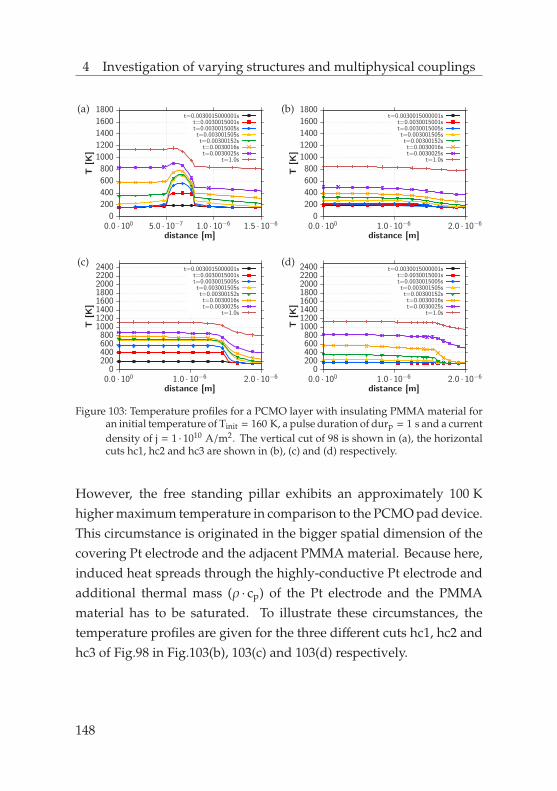
4 Investigation of varying structures and multiphysical couplings
0
200
400
600
800
1000
1200
1400
1600
1800
0.0 · 100 5.0 · 10−7 1.0 · 10−6 1.5 · 10−6
T[K
]
distance [m]
t=0.0030015000001st=0.0030015001st=0.0030015005st=0.003001505st=0.00300152st=0.0030016st=0.0030025s
t=1.0s
(a)
0
200
400
600
800
1000
1200
1400
1600
1800
0.0 · 100 1.0 · 10−6 2.0 · 10−6
T[K
]
distance [m]
t=0.0030015000001st=0.0030015001st=0.0030015005st=0.003001505st=0.00300152st=0.0030016st=0.0030025s
t=1.0s
(b)
020040060080010001200140016001800200022002400
0.0 · 100 1.0 · 10−6 2.0 · 10−6
T[K
]
distance [m]
t=0.0030015000001st=0.0030015001st=0.0030015005st=0.003001505st=0.00300152st=0.0030016st=0.0030025s
t=1.0s
(c)
020040060080010001200140016001800200022002400
0.0 · 100 1.0 · 10−6 2.0 · 10−6
T[K
]
distance [m]
t=0.0030015000001st=0.0030015001st=0.0030015005st=0.003001505st=0.00300152st=0.0030016st=0.0030025s
t=1.0s
(d)
Figure 103: Temperature profiles for a PCMO layer with insulating PMMA material foran initial temperature of Tinit = 160 K, a pulse duration of durp = 1 s and a currentdensity of j = 1 · 1010 A/m2. The vertical cut of 98 is shown in (a), the horizontalcuts hc1, hc2 and hc3 are shown in (b), (c) and (d) respectively.
However, the free standing pillar exhibits an approximately 100 Khigher maximum temperature in comparison to the PCMO pad device.This circumstance is originated in the bigger spatial dimension of thecovering Pt electrode and the adjacent PMMA material. Because here,induced heat spreads through the highly-conductive Pt electrode andadditional thermal mass (ρ · cp) of the Pt electrode and the PMMAmaterial has to be saturated. To illustrate these circumstances, thetemperature profiles are given for the three different cuts hc1, hc2 andhc3 of Fig.98 in Fig.103(b), 103(c) and 103(d) respectively.
148

4 Investigation of varying structures and multiphysical couplings
The horizontal cut hc1 shows, that for every time point, almost notemperature gradient exists from the axis of symmetry towards theside. On the contrary, the horizontal cut hc2 exhibits a significanttemperature decrease from the actively heated PCMO material to thenon actively heated PCMO material. Moreover, horizontal cut hc3shows, that already after 1 µs of heating, a significant temperaturegradient exists within the Pt top electrode. Thus, every horizontalcut illustrates that heat is spread to the side. Consequently, themean temperature in the PCMO layer is less than for the freestanding pillar and hence, the electric resistance must be slightlyhigher for the PCMO pad device in comparison to the free standingpillar. A corresponding temperature visualization of Fig.103 is givenin Fig.104. This visualization helps to understand the previouslymentioned temperature developments and completes the picture ofheat spread.
149

4 Investigation of varying structures and multiphysical couplings
(a) (e)
(b) (f)
(c) (g)
(h) (k)
Figure 104: Temperature visualization for the PCMO pad device with insulating PMMAmaterial [cf. Fig.94(b)]. The conditions are: Initial temperature of Tinit = 160 K,a pulse duration of durp = 1 s and a current density of j = 1 · 1010 A/m2. Shownare the respective time steps of Fig.103.
150

4 Investigation of varying structures and multiphysical couplings
1
10
100
1000
10000
107 108 109 1010
R(T
)[Ω]
j [A/m2]
0250500750
107 1010
∆T
[K]
durp = 1µsdurp = 1s
(a)
1
10
100
1000
10000
107 108 109 1010
R(T
)[Ω]
j [A/m2]
0250500750
107 1010
∆T
[K]
durp = 1µsdurp = 1s
(b)
1
10
100
1000
10000
107 108 109 1010
R(T
)[Ω]
j [A/m2]
0250500750
107 1010
∆T
[K]
durp = 1µsdurp = 1s
(c)
Figure 105: Temperature dependent resistance behavior for the free standing PCMOpillar without the Kleindiek contact [cf. Fig.94(c)]. The ambient temperaturesare (a) 300 K, (b) 230 K and (c) 160 K. The insets contain the relative temperatureincrease ∆T within the heating pulse.
As result, the respective resistance behavior is shown in Fig.105 for thefree standing PCMO pillar without the Kleindiek contact [cf. Fig.94(c)]as example. The electric resistance of the pillar is calculated by Eq.4.21with the maximum occurring mean temperature, which we find at theend of the induced electric pulse [cf. Fig.97].First, the initial temperature of Tinit = 300 K is considered. Theelectric resistance remains almost the same until a current densityof j = 1 · 108 A/m2 is applied. From then on, the electric resistancedecreases extremely with increasing current density. Essentially,the decrease in electric resistance occurs when the temperature alsoincreases significantly.
151

4 Investigation of varying structures and multiphysical couplings
The respective temperature amplitudes are indicated in the insets ofFig.105. This tendency appears for both, a 1 µs and 1 s induced currentpulse. However, in general, the resistance always stays slightly higherfor a 1 µs than for a 1 s pulse. This implies in turn, that the majorheating takes place within 1 µs. Second, the initial temperatureof Tinit = 230 K is considered. Similar to an initial temperature ofTinit = 300 K, the electric resistance remains almost the same forsmall current densities. However, the decrease in electric resistancealready occurs for smaller current densities in comparison to theinitial temperature of Tinit = 300 K. Third, the initial temperatureof Tinit = 160 K is considered. Here, the electric resistance alreadydecreases for small current densities in comparison to the previousinitial temperatures. As result, the electric resistance decreasestremendously for every initial temperature at high current densities.A numerical comparison of the different temperature dependentelectric resistivity values is given in Tab.4 for the different pillarconfigurations and the pad device [cf. Fig.94]. In general, the pillarconfigurations and the pad device exhibit the same temperaturedependent resistivity behavior with increasing current densities.However, evidently the pad device always results for increasingcurrent densities in the highest remaining electric resistanceafterwards the respective pulses were applied.As an overall result, the previous given simulations prove thatextremely high temperatures occur for high current densities.Consequently, is seems plausible that such high temperatures couldinitiate oxide migration and hence assist the switching mechanismthermally.
152

4 Investigation of varying structures and multiphysical couplings
Pilla
rPi
llar
wit
hPa
dtu
ngst
en(W
)con
tact
cf.F
ig.9
4(c)
cf.F
ig.9
4(c)
cf.F
ig.9
4(d)
T ini
t[K
]j[
A/m
2 ]∆
T[K
]R
(T)[
Ω]
∆T
[K]
R(T
)[Ω
]∆
T[K
]R
(T)[
Ω]
300
1·10
70.
0431
2.06
0.04
312.
060.
0331
2.09
1·10
83.
9229
3.73
3.92
293.
783.
3529
6.30
1·10
911
1.67
84.3
911
1.76
84.3
710
2.55
91.5
11·10
1088
4.45
6.62
884.
616.
6281
7.81
7.26
230
1·10
70.
1712
90.6
60.
1712
90.6
70.
1412
91.5
31·10
812.5
894
7.54
12.6
094
7.92
11.0
898
2.04
1·10
915
0.45
113.
1315
0.46
113.
0814
0.47
125.
411·10
1092
4.04
6.90
924.
076.
9085
7.12
7.61
160
1·10
72.
0915
676.
862.
0915
680.
411.
8015
911.
981·10
840.8
930
93.0
340.8
930
91.7
338.0
934
07.3
21·10
919
6.86
145.
6719
6.85
145.
6718
6.13
165.
191·10
1096
5.32
7.18
965.
417.
1889
8.10
7.96
Tabl
e4:
Com
pari
son
ofth
edi
ffer
ent
occu
rrin
gte
mpe
ratu
ream
plit
udes
and
resu
ltin
gre
sist
ance
sw
ithi
na
1s
heat
ing
puls
efo
rth
edi
ffer
entP
CM
Opi
llars
[cf.
Fig.
94].
153

5 Methodology to determine the isotropic
and anisotropic thermal conductivity
The analysis of the previously investigated geometry structuresexhibits to some extent completely different ∆T -line behaviors incomparison to classic 3ω-method configurations. Thus, the offsetmodel and slope methods are no longer applicable to determine thethermal conductivity since they are based on analytic descriptionswhich are no longer valid for these systems. Hence, a new method isrequired, which can be applied on various geometries, frequencies andmaterial combinations. In this work, a new methodology is presentedwhich combines the advantages of different structures and frequenciesto determine the isotropic and anisotropic thermal conductivity.
5.1 General methodology
This methodology involves experiments and numerical analysis forthe investigated materials. The general procedure is shown in Fig.106.After the sample is fabricated, a 3ω-measurement is performed for theinvestigated material first. Second, the presented Finite Element Modelis used to simulate the exact given geometry configuration. The FiniteElement simulations obtain the temperature amplitude ∆T as output.Third, the Neural Network is established. The Neural Network has tobe trained in the range of the expected thermal conductivity. Moreover,the more dependencies are known, the better is the solution of theNeural Network in the end. In this work, the calculated ∆T for a giventhermal conductivity is used to train a Neural Network. Essentially, theNetwork is trained in the opposite direction which means the Networklearns the dependencies for given ∆T ’s to κ.
155

5 Methodology to determine the thermal conductivity
Figure 106: Illustration of the general procedure to determine thermal conductivities.The ‘Sample Preparation’ and ‘Measurement’ pictures are taken from themeasurement setup, established by our project partners.
Since the Network can interpolate, it is able to solve the InverseProblem. However, as shown in previous sections, anisotropic thermalconductivity variations can result for some geometry configurationsin different characteristics in the ∆T -lines. An example for thisbehavior is given in Fig.86(b) for the long heater configuration ofthe 6-pad heater structure. Comparing in this plot the black andblue ∆T -lines exhibits, that the black line is above the blue linefor low frequencies but turns around for high frequencies. If weassume that only one anisotropic thermal conductivity combinationcan exist for a clear defined ∆T -line, this configuration of the 6-pad
156
5 Methodology to determine the thermal conductivity
heater structure can be used to determine the anisotropic thermalconductivity within one step (κx, κy). Therefore, this work appliesa new approach by using the information of different ∆T -lines ingeneral over a defined frequency regime instead of either the slopeor the axis intercept. However, some configurations are not suitableto determine the cross- and in-plane thermal conductivity within onestep. In this case, still two measurements and two Neural Networksare needed to identify the cross- and in-plane thermal conductivityseparately because the respective sensitivity is too small. The laststep combines the temperature amplitude, measured in experimentswith the established Neural Networks to identify the correspondentthermal conductivities. By this procedure, we do not need toemploy any restricting assumptions that may be needed to deriveanalytic solutions. Consequently, we can investigate many systemconfigurations.
5.2 Neural Network and Inverse Problem
A Neural Network constitutes a mathematical instrument to representand approximate arbitrary dependencies where no explicit analyticalexpressions are available [cf. 73, 140]. Its definition is originatedin natural nervous systems and brains of humans and animals.Information of nervous systems are processed by a big number ofsimple and parallel working units [96]. These units are so-calledNeurons. Whether information is exchanged or not, depends onactivation signals.Just as a human brain must learn dependencies in general, a NeuralNetwork must be trained on a certain data basis before an outcomecan be predicted.
157

5 Methodology to determine the thermal conductivity
The amount of data, the formatting and eventual incorporatedmathematical background limits the ‘knowledge and accuracy’ of theNeural Network. Subsequent to the training process, the NeuralNetwork is able to predict the previously unknown value as outcome.The Neural Networks which we apply in this work are developedby S. Scherrer-Rudiy [140] and especially N. Huber [73]. Just asthis work focuses on thermal conductivities of thin layer materials,the fundamental work of N. Huber was used to identify mechanicalproperties of thin layer materials in [73] and mechanical properties ingeneral by E. Tyulyukovskiy [154] and S. Scherrer-Rudiy [140].In the following, the working principle of the Neural Network isdescribed. The mathematical treatment of a Neuron is shown inFig.107.
Figure 107: Illustration of the mathematical modeled Neuron.
Here,Xj is the input vector of the regarded Neuron. The entities of theinput vector are multiplied by the synaptic weightsWij and summedup. The activation of the Neuron, and thus whether or not the outputvectorYi is greater than zero, depends finally on the activation functionQ. Possible activation function examples are step functions or tangenthyperbolicus. A Neural Network contains several of such Neurons indifferent layers. In this work, a conventional Feed-Forward Networkis used to describe the dependencies between temperature amplitude
158

5 Methodology to determine the thermal conductivity
and thermal conductivities.42 The Neural Network scheme is shownin Fig.108.
Figure 108: Illustration of a general Neural Network scheme with three different layers.
A Neural Network must contain at least one input and one output layer.Existing layers in between are so-called ‘hidden layers’. While thenumber of in- and output values in the respective vector are predefinedby the problem which has to be solved, the numbers of hidden layersand internal Neurons are subject to change. In general, more hiddenlayers and internal Neurons are necessary if the dependencies arecomplex.Neural Networks learn the dependencies of given training examplesby adapting the synaptic weightsW so that the given training exampleis reproduced. The training examples contain a vector pair with theinput and output values. The training process uses an optimizationprocedure for the object function
S(W) = G(W) + E(W) . (5.1)
42A Feed-Forward Network contains only relations from the previous layer to the nextlayer. This means, no back loop exists from the next layer to the previous layer [96].
159

5 Methodology to determine the thermal conductivity
The object function S(W) consists of an error term G(W) and aregulation term E(W).43 The aim of the optimization is to findoptimum synaptic weights, so that the difference between the outputvector and the training example is as small as possible. By minimizingthe object function, the Neural Network is trained. Therefore, agradient method is applied for an iterative improvement of thesynaptic weightsW so that
WT+1 =WT
− η∇S(W) . (5.2)
Here, WT+1 is the next iterative synaptic weight, WT is the actualsynaptic weight, η is an empirically determined scaling parameter and∇S(W) is the applied gradient on the object function S(W).After sufficient iterative improvements, an optimum W is obtainedfor which the Neural Network has a minimum error.44 However, thetraining requires caution, since too much training or a local minimumfalsifies the result. Thus, the Neural Network has to be subsequentlyvalidated. Therefore, a known data set for in- and output vectorsmust be excluded from training and checked with the establishedNeural Network afterwards. Finally, the Neural Network can beused to predict the desired unknown values. In general, the qualityof the result depends primarily on the quantity and quality of theused training examples. This means first: A sufficient fine pattern ofdata points (vectors) must be given for the training process. Second,the Network’s prediction towards the borders of the numerical datacontains a higher uncertainty since these data points are surroundedby less training data points.
43Detailed information about the object function is given by S. Scherrer-Rudiy [140]44Detailed information about the error is given by S. Scherrer-Rudiy [140].
160

5 Methodology to determine the thermal conductivity
Third, predictions beyond the trained data basis are rather less reliable.At last, the quality of the Network decreases for wrong vector pairs, ifthey are used for training.45
In this work, Neural Networks are trained in a way, that they learn thethermal conductivities corresponding to the temperature amplitudes,so that
X(∆T )→ Y(κ) . (5.3)
Thus, the Network can use the temperature amplitudes which aremeasured in experiments and interpolate the corresponding thermalconductivities.
45Detailed descriptions and discussions about the quality of Neural Networks is givenin [73], [140] and [96].
161

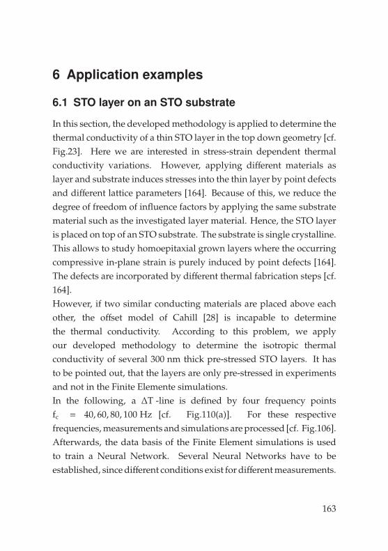
6 Application examples
6.1 STO layer on an STO substrate
In this section, the developed methodology is applied to determine thethermal conductivity of a thin STO layer in the top down geometry [cf.Fig.23]. Here we are interested in stress-strain dependent thermalconductivity variations. However, applying different materials aslayer and substrate induces stresses into the thin layer by point defectsand different lattice parameters [164]. Because of this, we reduce thedegree of freedom of influence factors by applying the same substratematerial such as the investigated layer material. Hence, the STO layeris placed on top of an STO substrate. The substrate is single crystalline.This allows to study homoepitaxial grown layers where the occurringcompressive in-plane strain is purely induced by point defects [164].The defects are incorporated by different thermal fabrication steps [cf.164].However, if two similar conducting materials are placed above eachother, the offset model of Cahill [28] is incapable to determinethe thermal conductivity. According to this problem, we applyour developed methodology to determine the isotropic thermalconductivity of several 300 nm thick pre-stressed STO layers. It hasto be pointed out, that the layers are only pre-stressed in experimentsand not in the Finite Elemente simulations.In the following, a ∆T -line is defined by four frequency pointsfc = 40, 60, 80, 100 Hz [cf. Fig.110(a)]. For these respectivefrequencies, measurements and simulations are processed [cf. Fig.106].Afterwards, the data basis of the Finite Element simulations is usedto train a Neural Network. Several Neural Networks have to beestablished, since different conditions exist for different measurements.
163

6 Application examples
The varying conditions are: The power per length and heater’s heightvary between P/L = 5 − 7.5 W/m and a = 100 − 300 nm respectively.The thermal conductivity of the substrate varies between differentSTO samples and varies especially for different ambient temperatures.The heat capacity of the STO layer and the substrate also changeswith different ambient temperature [51]. On the contrary, the heater’swidth 2b = 10 µm and the substrate thickness ds = 1 mm is the samethroughout every experiment. Consequently, various Finite Elementsimulations are realized, to take the previously given conditions intoaccount. In this application study, only the temperature field isconsidered. While we assume the boundaries Γ1−3 to be adiabatic,we take into account a heat transfer from the substrate to the mountat boundary Γ4 by Eq.4.4 [cf. Fig.109]. Moreover, all materials areassumed to be isotropic. Hence, the partial differential equation for thesubstrate and for the heater are given by Eq.3.1 and Eq.3.2 respectively.The partial differential equation for the investigated layer materialwrites to
Ωlay :∂2Tlay
∂x2 +∂2Tlay
∂y2 −1
Dlay
∂Tlay
∂t= 0 . (6.1)
The training of the Neural Network is done first by declaring fourtemperature amplitude values as an input vector. These values arethen correlated to the output vector, which is the thermal conductivity.A schematic overview is given in Fig.110(b). Here, the training appliestwo hidden layers and between 5 to 30 internal Neurons. It turned outthat the object function S(W) can be minimized more efficiently bymultiplying the ∆T values by 10, so that the input vectors X(∆T ) andoutput vectorsY(κ) are on the same order of magnitude.
164

6 Application examples
Ωs
ΩH
Ωlay
Γ1
Γ2
Γ3
Γ4
Figure 109: Considered system for the Finite Element simulation.
In this study, we investigate the thermal conductivity at roomtemperature T0 = 300 K for different pre-strained layers first. Anexample for several simulated data pairs is plotted together withthe respective measurement in Fig.110(c) for a strain of ε = 0, 62%.The result of the Neural Network identification for the correspondingthermal conductivity is shown in Fig.111(a). Moreover, this figurecontains the results for different pre-strained layers down to ε =
0, 17%. This study at room temperature exhibits, that the thermalconductivity decreases from approximately 10 W/mK at ε = 0, 17 %to approximately 5 W/mK at ε = 0, 62 %. Hence, the thermalconductivity is reduced by 50% and thus decreases significantly.Second, the temperature dependence on pre-strained layers isinvestigated. An example for several simulated data pairs isplotted together with the respective measurement in Fig.110(d) fora temperature of T0 = 200 K and a strain of ε = 0, 62 %. The result forthe corresponding thermal conductivity is shown in Fig.111(b) togetherwith the results for measuring temperatures down to 40 K.
165

6 Application examples
In this figure, it is shown that, while the thermal conductivity of theunstrained substrate increases slightly towards a temperature of 40 K,the thermal conductivity of the thin STO layer decreases further. Here,a thermal conductivity around κ ≈ 1 W/mK is determined at 40 K. Asan overall consequence, the previous results indicate a tremendousimpact of strain on the thermal conductivity of thin STO layers. Fordetailed explanation, see Wiedigen et al.[164].
(a) (b)
5.2
5.4
5.6
5.8
6.0
6.2
6.4
40 60 80 100
∆T·1
0[K
]
Frequency fc [Hz]
κ at T0 = 300[K]
ε = 0.62%
Simulation κ = 5.0 [W/mK]Simulation κ = 5.5 [W/mK]Simulation κ = 6.0 [W/mK]Simulation κ = 6.5 [W/mK]
Measurement
(c)
5.6
5.8
6.0
6.2
6.4
6.6
6.8
7.0
40 60 80 100
∆T·1
0[K
]
Frequency fc [Hz]
κ at T0 = 200[K]ε = 0.62%
Simulation κ = 3.0 [W/mK]Simulation κ = 3.5 [W/mK]Simulation κ = 4.0 [W/mK]Simulation κ = 4.5 [W/mK]Simulation κ = 5.0 [W/mK]
Measurement
(d)
Figure 110: (a) Schematic assignment of thermal conductivities, based on a temperatureamplitude over frequency plot. (b) Sketch of the Neural Network for thethermal conductivity determination. (c) Example of the line identification fora measurement at a strain of ε = 0, 62 % within the numerical simulation database values for an ambient temperature of T0 = 300 K and an identified thermalconductivity of κlay = 5.48 W/mK and (d) an identified thermal conductivity ofκlay = 4.27 W/mK at T0 = 200 K.
166

6 Application examples
4
5
6
7
8
9
10
11
12
0.1 0.2 0.3 0.4 0.5 0.6 0.7
κ[W
/mK]
ε [%]
T0 = 300[K]
Determined thermal conductivity κlay
(a)
0.0
2.5
5.0
7.5
10.0
12.5
15.0
17.5
20.0
0 50 100 150 200 250 300 350
κ[W
/mK]
Temperature T [K]
ε = 0.62 [%]
Determined thermal conductivity κlaySubstrate reference κsubs
(b)
Figure 111: (a) Results for the determined strain dependent thermal conductivity atT0 = 300 K. (b) Results for the determined strain and temperature dependentthermal conductivity at ε = 0, 62 % in comparison to the applied and unstrainedSTO substrate.
167

6 Application examples
6.2 Bottom electrode geometry
In this section, the bottom electrode geometry is used incombination with the developed methodology to determine thethermal conductivity of a thin poorly-conductive STO layer. However,as shown in Sec.4.2.2, a heater substrate platform is rather insensitivefor poor conductive layers on top. Due to this problem, we apply herea heat sink on top of the layer material to increase the sensitivityfor the 3ω-method to determine the thermal conductivity of thepoorly-conductive layer. A scanning electron microscopy image isshown in Fig.112 for the bottom electrode geometry configurationwhich we investigate in this section.
Figure 112: SEM image of the bottom electrode geometry. The SEM image was taken byour project partners of the University of Gottingen. The Pt layer on top of the Cusink is not present for the 3ω-measurement. It exists only to protect the bottomelectrode geometry for the SEM imaging process.
In the following, the manufacturing and measurement processare described first and afterwards, the numerical simulations areexplained.First, the heater substrate platform is fabricated and a 3ω-measurementis performed to determine the thermal conductivity of the substrate [cf.Fig.113(a)]. Here, a Pt heater with a height of a = 203 nm and a width
168

6 Application examples
of 2b = 10 µm is applied on top of a 1 mm thick YSZ substrate.46
Second, the thin STO layer is placed on top of the heater substrateplatform and a 3ω-measurement is performed [cf. Fig.113(b)]. Here,the thin STO layer on top is at least as wide, as the substrate is thick.Hence, the STO layer is considered as full covering. The thickness ofthe STO layer is dlay = 221 nm.Third, the Cu heat sink is placed on top of the layer by two depositionsteps. Afterwards, a 3ω-measurement is performed for this stackedmaterial combination [cf. Fig.113(c)]. Due to the fabrication process,the Cu heat sink on top has a width of 2bsin = 500 µm and aheight of dsin = 1.454 µm. In this section, every measurement andsimulation applies a power per length of P/L = 5 W/m and measuringfrequencies of fc = 100, 200, 400, 600, 800, 1000 Hz. Fig.114 containsthe temperature amplitude measured in experiments at the definedfrequency points for the pure heater substrate platform (Pt-YSZ), theheater substrate platform with the STO layer on top (STO-Pt-YSZ)and the heater substrate platform with the additional heat sink on top(Cu-STO-Pt-YSZ).For this application example, the numerical analysis can be dividedinto two major steps. In the first step, the thermal conductivityof the substrate is determined, and in the second step, the thermalconductivity of the investigated layer material is identified.To determine the thermal conductivity of the substrate, the pure heatersubstrate platform is considered [cf. Fig.113(a)]. For this system, FiniteElement simulations generate a data basis for thermal conductivityvariations of the substrate first. In this application study, only thetemperature field is considered.
46In this section, every material placed on top of the heater substrate platform isfabricated by a sputtering process.
169
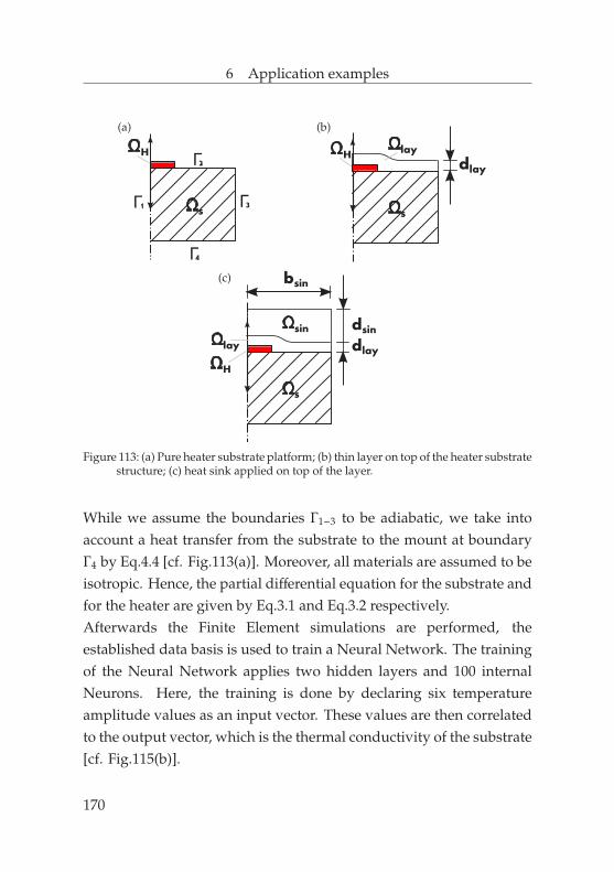
6 Application examples
Γ
Ωs
4
Γ1 Γ3
Γ2ΩH
(a)
Ωs
ΩHΩlay
dlay
(b)
Ωs
ΩH
Ωlay dlay
Ωsin dsin
bsin(c)
Figure 113: (a) Pure heater substrate platform; (b) thin layer on top of the heater substratestructure; (c) heat sink applied on top of the layer.
While we assume the boundaries Γ1−3 to be adiabatic, we take intoaccount a heat transfer from the substrate to the mount at boundaryΓ4 by Eq.4.4 [cf. Fig.113(a)]. Moreover, all materials are assumed to beisotropic. Hence, the partial differential equation for the substrate andfor the heater are given by Eq.3.1 and Eq.3.2 respectively.Afterwards the Finite Element simulations are performed, theestablished data basis is used to train a Neural Network. The trainingof the Neural Network applies two hidden layers and 100 internalNeurons. Here, the training is done by declaring six temperatureamplitude values as an input vector. These values are then correlatedto the output vector, which is the thermal conductivity of the substrate[cf. Fig.115(b)].
170

6 Application examples
0.00
0.40
0.80
1.20
1.60
2.00
2.40
100 200 400 600 1000
∆T
[K]
Frequency fc [Hz]
Measurement: Pt-YSZSTO-Pt-YSZ
Cu-STO-Pt-YSZ
Figure 114: Temperature amplitudes measured in experiments at the defined frequencypoints for the pure heater substrate platform (Pt-YSZ), the heater substrateplatform with the STO layer on top (STO-Pt-YSZ) and the heater substrateplatform with the additional heat sink on top (Cu-STO-Pt-YSZ). Here, everymeasurement line is the arithmetic mean value of three different measurementsat exactly the same sample.
Subsequently, the established Neural Network is used to solvethe Inverse Problem and identify the thermal conductivity of thesubstrate from the temperature amplitudes measured in experiments.This identification is shown in Fig.115(c). The identified thermalconductivity of the substrate is κs = 2.10 W/mK.47
In the second step, the thermal conductivity of the layer material isidentified. Therefore, Finite Element simulations are processed forthe stacked material combination of Fig.113(c). Thus for the heatersubstrate platform with layer material and heat sink on top. Here,the previously determined thermal conductivity of the substrate isused. In this second step, the thermal conductivity of the investigatedSTO layer material is varied in the Finite Element simulations. Here,we also assume every outer boundary to be adiabatic except for thesubstrate mount, where we take into account again a heat transfer fromthe substrate to the mount.
47The literature value for the thermal conductivity of YSZ is κ = 1.8 W/mK.
171

6 Application examples
Also here, every material is assumed to be isotropic. The partialdifferential equation for the substrate and for the heater are givenby Eq.3.1 and Eq.3.2. The partial differential equations for the heatsink and the investigated layer material write to
Ωsin :∂2Tsin
∂x2 +∂2Tsin
∂y2 −1
Dsin
∂Tsin
∂t= 0 , (6.2)
Ωlay :∂2Tlay
∂x2 +∂2Tlay
∂y2 −1
Dlay
∂Tlay
∂t= 0 . (6.3)
Based on the Finite Element simulations, a second Neural Networkis established. Again, the training of the Neural Network is doneby declaring six temperature amplitude values as an input vector.These values are then correlated to the output vector, which is nowthe thermal conductivity of the layer material. Finally, this secondNeural Network is used to solve the Inverse Problem and identify thethermal conductivity of the investigated STO layer material from thetemperature amplitudes measured in experiments. The correspondingidentification is shown in Fig.115(d). The identified thermalconductivity of the layer is κlay = 1.2 W/mK. This identified thermalconductivity of the STO layer seems rather small in comparison tothe other STO layers of this work. However, in case of the bottomelectrode, the placed STO layer is grown polycrystalline. Hence, webelieve that the thermal conductivity should be significantly smaller.However, as shown in Sec.4.2.3, this bottom electrode geometryconfiguration is especially sensitive and suitable to determine poorcross-plane thermal conductivities. Consequently, this identifiedthermal conductivity is the cross-plane thermal conductivity of thelayer material. Moreover, this application example proofs that thethe bottom electrode geometry can be used to determine the thermalconductivity of poorly-conductive layer materials in combinationwith the established methodology of this work.172

6 Application examples
(a) (b)
1.0
1.2
1.4
1.6
1.8
2.0
100 200 400 600 800 1000
∆T
[K]
Frequency fc [Hz]
Simulation κ = 2.00 [W/mK]Simulation κ = 2.05 [W/mK]Simulation κ = 2.10 [W/mK]Simulation κ = 2.15 [W/mK]Simulation κ = 2.20 [W/mK]
Measurement
(c)
0.20
0.25
0.30
0.35
0.40
0.45
100 200 400 600 800 1000
∆T
[K]
Frequency fc [Hz]
Simulation κ = 0.8244 [W/mK]Simulation κ = 0.9274 [W/mK]Simulation κ = 1.0305 [W/mK]Simulation κ = 1.1336 [W/mK]Simulation κ = 1.2366 [W/mK]
Measurement
(d)
Figure 115: (a) Schematic assignment of thermal conductivities, based on a temperatureamplitude over frequency plot. (b) Sketch of the Neural Network for the thermalconductivity determination. (c) Example of the line identification for the heatersubstrate platform measurement within the numerical simulation data base valuesfor an identified thermal conductivity of κs = 2.10 W/mK and (d) an identifiedthermal conductivity of κlay = 1.2 W/mK for the investigated layer material.
173


7 Summary
This work aims to deepen the understanding of thermal conduction innanostructured materials to design new thermoelectrics with higherefficiency than these materials exhibit today. However, therefore ameasurement technique is required where we focus on the 3ω-method.Thus, the primary objectives of this work are to examine macroscopicinfluence factors within a 3ω-measurement, to develop new geometricmeasuring configurations in order to determine the isotropic andanisotropic thermal conductivity, and to establish a new evaluationmethodology. Since thermoelectricity and the 3ω-method are basedon heat propagation, the fundamentals of heat conduction are derivedin the beginning.
The second section elucidates the concept, basic principles, andgeometric configurations of the 3ω-method. Existing literatureis reviewed and several solutions of the top down geometry arecompared. The range of applicability is also examined. Moreover,fundamental work for the bottom electrode geometry is introducedand the potential use of a new heater substrate platform is presented.
The third section presents the governing equations of the usedFinite Element Model. Here, the equations are derived in a partialdifferential sense. The interaction between the distinct macroscopicinfluence factors are explained and the respective considerationis motivated. This includes the temperature dependent electricresistivity of the heater, the electromagnetic induced skin effect, andthe mechanical displacements within a measurement. Moreover,details for the time-dependent analysis are given and a mesh-block
175

7 Summary
building system is presented to obtain a pre-defined mesh in order toachieve high precision analysis.
The fourth section applies the presented Finite Element Modelon various geometric structures. Moreover, macroscopic influences,which are not commonly adressed in literature are examined. Forinstance, a temperature dependent electrical resistivity changes thetemperature amplitude on the 4th decimal place. Taking into accountthermal expansion can have an impact on the 3rd decimal place. Onthe contrary, the occurring skin effect has almost no influence on thetemperature amplitude for frequencies up to 1 MHz.Furthermore, mono- and multilayer configurations are investigated.First, analytic descriptions are compared to the Finite Elementsolution and differences are identified. In comparison to the givendescriptions, the Finite Element solution appears to be the most precisesolution at high frequencies. Hence, the performed simulations allowunderstanding the system behavior especially in the high frequencyregime. Second, in order to determine the anisotropic thermalconductivity, different heater geometries are studied on top of mono-and multilayer configurations. Here, also non-classic layer substrateconfigurations are studied where poorly-conductive substrates areapplied.Additionally, a bottom electrode geometry is investigated todetermine the isotropic and anisotropic thermal conductivity ofnanoscale samples. Here the bottom electrode is especially examinedfor the anisotropic thermal conductivity determination of thin layers.This includes the application of heat sinks on top of the layer.In principal, the investigated heat sink configurations allow thedetermination of the anisotropic thermal conductivity. However,
176
7 Summary
since fabrication seems rather complicated, these configurations areinconvenient to determine the anisotropic thermal conductivity.We think, that membrane structures are the solution to determinethe anisotropic thermal conductivity. Therefore, these structuresare investigated in this work. First, two-dimensional models arestudied to understand the general system behavior. This includesdifferent geometrical properties of the membrane, the applied powerper length, and heat loss by radiation. Second, a three-dimensionalmodel is developed in this work. The so-called 6-pad heaterstructure allows to determine for both materials, STO and PCMO, thein-plane thermal conductivity. Moreover, if a moderately-conductivemembrane could be applied, the 6-pad heater structure would alsoprovide the possibility to determine the in-plane thermal conductivityas well as the cross-plane thermal conductivity for an extremelypoorly-conductive layer material.Since micro- to nanoscale PCMO samples exhibit a change in electricresistance by electric stimulation (resistive switching), such as shortimpulse induced high current densities, this material has also beeninvestigated in pillar geometries. Here the simulations provide asubstantial contribution to understand the temperature developmentand thus the electric resistivity behavior in these experiments.
The fifth section presents a new methodology to determine thethermal conductivity, where no analytic solution is available.Since Finite Element simulations and experimental measurementsresult in temperature amplitudes, a procedure is necessary tomerge simulations and experiments for the thermal conductivitydetermination. In this work, Finite Element simulations and NeuralNetworks are combined to evaluate experimental measurements.
177

7 Summary
Here, the Neural Networks are based on Finite Element results andconnect experimental measurements with their respective simulatedthermal conductivities. Hence, this allows to solve the Inverse Problemand thus determine the desired sample properties. The presentedmethodology can be applied to various geometric configurations suchas the bottom electrode or the 6-pad heater structure. However, classicconfigurations can also be studied, where no offset model or slopemethod is applicable.
The last section is dedicated to two application example of the newmethodology. The first example applies the developed methodologyon a top down geometry. Here, a thin STO layer is investigated forstress-strain dependent thermal conductivity. To exclude an influencethrough the substrate by different lattice parameters of layer andsubstrate, the STO layer is deposed by a sputtering process on topof an STO substrate. Hence, a top down configuration exists, whereno clear defined offset occurs. Based on the precise Finite Elementsimulations and the new developed methodology, it is possible tostudy the influence of strain on the thermal conductivity. As result,the thermal characterization exhibits a strong influence of strain onthe thermal conductivity of thin STO layer material.The second example applies the developed methodology on a bottomelectrode geometry where a heat sink is applied on top of theinvestigated layer material. This example proofs the feasibility for abottom electrode geometry to determine the thermal conductivity ofa poorly-conductive thermoelectic material.
178
7 Summary
Overall, this thesis presents a comprehensive understanding onmacroscopic factors, influencing Joule heating measurements at smallscales. The simulations quantify the absolute temperature andtemperature amplitude for structures used in 3ω-measurements andin pillar and pad structure experiments. Based on these simulations,new geometric configurations are developed for the 3ω-method andcombined with a new methodology to determine the isotropic andanisotropic thermal conductivity. Finally, the developed evaluationmethodology can be generalized and consequently be applied to awider range of Joule heating applications for characterizing thermalproperties of small scale materials.
179


Appendix A. Detailed information on formula
A.1 Modulated voltage
U = I ·R (A.11)
= I0 cos(ωt) · [Rav + ∆R cos(2ωt + ς)]
= I0Rav cos(ωt) + I0∆R cos(ωt) cos(2ωt + ς)
= I0Rav cos(ωt) + I0∆R12
[cos(ωt − (2ωt + ς)) + cos(ωt + (2ωt + ς))]
= I0Rav cos(ωt) + I0∆R12
[cos(ωt) cos(2ωt + ς)
+ sin(ωt) sin(2ωt + ς) + cos(ωt) cos(2ωt + ς)
− sin(ωt) sin(2ωt + ς)]
U = I0Rav cos(ωt) +I0∆R
2(cos(3ωt + ς) + cos(ωt + ς)) (A.12)
181
Appendix A. Detailed information on formula
A.2 Information about the approximate solution
Cahill [28] proposed an approximate solution for the case that thethermal penetration depth is large in comparison to the half heaterwidth (q−1
b → bq 1). He sets the limits of the integral from 0to 1/b and assumes that
sin2(kb)
(kb)2 = 1 . (A.23)
Thus, Eq.2.17 writes now as:
∆TCh =
P0
Lπκs
∫ 1/b
0
1√k2 + q2
dk =P0
Lπκs· ln
∣∣∣∣∣k +
√k2 + q2
∣∣∣∣∣1/b0
=P0
Lπκs
ln
∣∣∣∣∣∣1b +
√1
b2 + q2
∣∣∣∣∣∣ − ln∣∣∣q∣∣∣ =
P0
Lπκs
ln
1b +
√1b2 + q2
q
=P0
Lπκs
ln 1
bq+
√1
b2q2+ 1
=
P0
Lπκs
ln
1 +
√1 + bq2
bq
=P0
Lπκs
[−ln(bq) + ln(2)
]=
P0
Lπκs
−ln
b( D
i2ω
)− 12 + ln(2)
=
P0
Lπκs
[−
12
ln(b2
( Di2ω
)−1)+ ln(2)
]=
P0
Lπκs
[−
12
ln(b2 i2ω
D
)+ ln(2)
]=
P0
Lπκs
[−
12
ln(2ω) −12
ln(
ib2
D
)+ ln(2)
]=
P0
Lπκs
[−
12
ln(ω) −12
ln(
ib2
D
)−
12
ln(2) + ln(2)]
∆TCh =
P0
Lπκs
[−
12
ln(ω) −12
ln(
ib2
D
)+ const
](A.24)
182

Appendix A. Detailed information on formula
Here, the constant reads to
const = −12
ln(2) + ln(2) =12
ln(2) . (A.25)
Moreover, the temperature oscillation of the line heat source ∆T(r) fromEq.2.8 is also approximated in the following. If the distance r from theheat source is small in comparison to the thermal penetration depth,the modified Bessel function KB
0 can be approximated by neglectingterms of higher order so that KB
0 reads as [1, p. 375]
KB0 (s) = −
(ln
12
s + γ)· IB
0 (s) +1
4 s2
(1!)2 +(1 +
12
)·
( 14 s2)2
(2!)2 + ... (A.26)
= −ln(s) + ln(2) − γ . (A.27)
Here, γ = 0.577215... [37] is the Euler-Maschoneri constant and KB0
involves the modified Bessel function of first kind and zero order IB0 .48
48IB0 (s) = 1 +
14 s2
(1!)2 + ...
183
Appendix A. Detailed information on formula
With the latter approximation, the modified Bessel function KB0 reads
as
KB0 (qr) = −ln
( Di2ω
)− 12
· r
+ ln(2) − γ (A.28)
= −12· ln
[( Di2ω
)−1
· r2]
+ ln(2) − γ
= −12· ln
r2
Di2ω
+ ln(2) − γ
= −12·
[ln
(r2
D
)+ ln(i2ω)
]+ ln(2) − γ
= −12·
[ln(r2) − ln(D)
]−
12· ln(i2ω) + ln(2) − γ
=12·
[ln(D) − ln(r2)
]−
12· ln(i2ω) + ln(2) − γ
=12· ln
(Dr2
)−
12· ln (2ω) −
12· ln (i) + ln(2) − γ
=12· ln
(Dr2
)−
12· ln (2ω) −
12·π · i
2+ ln(2) − γ
KB0 (qr) =
12· ln
(Dr2
)−
12· ln(2ω) + ln(2) − γ −
π · i4
(A.29)
With the latter approximation of the modified Bessel function, thetemperature oscillation of Eq.2.8 writes to
∆T(r) =P0
Lπκs
[12· ln
(Dr2
)−
12· ln(2ω) + ln(2) − γ −
π · i4
]. (A.210)
184

Appendix A. Detailed information on formula
A.3 Definition of the skin depth and derivation ofdecoupled equations for the magnetic and electricfield intensity
First, the skin depth is introduced. The quantity of the skin depthdescribes the decrease of the current density with increasing distancefrom a surface of a material into it [130]. Per definition [130, p. 385],the skin depth δskin m writes to
δskin =
√2
ωσecµ. (A.311)
For high frequencies, the current is restricted to an extremely thin layernear the conductors surface [130].Second, the decoupled equations for the magnetic and electric fieldintensity are derived. Therefore, the following vector identity [cf. 76]is given under consideration of Eq.3.21:
∇ × ∇ ×H = ∇(∇ ·H) − ∇2H (A.312)
= ∇(µ−1· ∇ ·B) − ∇2H
= −∇2H (A.313)
185

Appendix A. Detailed information on formula
To get the wave equation, one can take the curl of the extendedAmpere’s law [Eq.3.18]. Thus, we get with the constitutive relations:
∇ × ∇ ×H = ∇ ×∂D∂t
+ ∇ × j (A.314)
−∇2H = ∇ ×
(ε∂E∂t
)+ ∇ × (σec ·E)
∣∣∣∣∣ cf. Eq.3.31, 3.29
= ε∂(∇ × E)∂t
+ σec(∇ × E)
= −ε
(∂2B∂t2
)+ σec
(−∂B∂t
) ∣∣∣∣∣ cf. Eq.3.20
= −εµ
(∂2H∂t2
)+ σecµ
(−∂H∂t
) ∣∣∣∣∣ cf. Eq.3.30
∇2H = εµ
(∂2H∂t2
)+ σecµ
(∂H∂t
)(A.315)
Equivalent to the previous equation, a similar derivation can be donefor Eq.3.20, the Faraday’s law, to derivate
∇2E = εµ
(∂2E∂t2
)+ σecµ
(∂E∂t
), (A.316)
for the electric field intensity. Thus both, the magnetic and electricfield intensity can be decoupled but still contain the informationabout the electro-magnetic waves. Considering the first and secondtime derivative [cf. Sec.3.1.2], iω and −ω2 respectively, Eq.A.315 andEq.A.316 develop to:
∇2H = (−ω2εµ + iωσecµ)H (A.317)
∇2E = (−ω2εµ + iωσecµ)E (A.318)
186

Appendix A. Detailed information on formula
This pair of equations are the so-called complex Helmholtz-equations.They can be written as
−∇2H + k2H = 0 , (A.319)
−∇2E + k2E = 0 , (A.320)
where k2 describes the complex wave. If terms of higher order areneglected, as mentioned in Sec.3.1.2, k2 reduces to
k2 = iωσecµ , (A.321)
and thus
k =√
iωσecµ . (A.322)
With the mathematical identity√
i = (1 + i)/√
2 we get
k =√ωσecµ · (1 + i) ·
1√
2=
√12·ωσecµ · (1 + i) . (A.323)
With the skin depth definition of Eq.A.311, Eq.A.323 becomes√12·ωσecµ · (1 + i) =
1δskin
(1 + i) . (A.324)
Consequently, the information of the skin depth is present in bothdecoupled complex Helmholtz-equations.
187
Appendix A. Detailed information on formula
A.4 Derivation for the complex Helmholtz-Equation
∇ ×H = iωD + J (A.425)
∇ ×H = iωD + σ · (−iωAj)
∇ ×H = iωε ·E + σ · (−iωAj)
∇ ×H = iωε · (−iωAj) + σ · (−iωAj)
∇ ×H = ω2ε ·Aj + σ · (−iωAj)
∇ ×B
µ= ω2ε ·Aj + σ · (−iωAj)
∇ × µ−1∇ ×Aj = ω2ε ·Aj + σ · (−iωAj)
(iωσ − ω2ε) ·Aj + ∇ × µ−1∇ ×Aj = 0 (A.426)
188

Appendix B. Material properties and
constants
Mat
eria
lel
ectr
ical
prop
erti
esth
erm
alpr
oper
ties
mec
hani
calp
rope
rtie
s
Pt% 0
=10.6·10−
8Ω
m[1
06]
κ=
71.6
W/m
K[1
06]
E=
1.65·10
11N/m
2[c
f.56
]α
=3·10−
31/
K∗
ρ=
2145
0kg/m
3[1
06]
ν=
0.39
[62]
µr
=1
+2.
57·10−
4 −[1
21]
c p=
130
J/kg
K[c
f.10
6]β
=9·10−
6[9
2]
STO
κ=
10.3
05W/m
K∗
E=
2.67·10
11N/m
2[1
64]
SrTi
O3
ρ=
5120
kg/m
3[4
5]ν
=0.
24[c
f.41
]c p
=54
4J/
kgK
[51]
β=
9.4·10−
6[c
f.14
9]
PCM
OR
(T)=
77.8
6/√
T·e12
72.2
6/TΩ
∗κ
=1.
58W/m
K[4
3]E
=3.
00·10
11N/m
2
Pr1−
xC
a xM
nO3
ρ=
570
kg/m
3[c
f.16
0]ν
=0.
4c p
=48
0J/
kgK
[cf.
102]
β=
10·10−
6
MgO
κ=
56.9
75W/m
K∗
E=
3.16·10
11N/m
2[1
16]
ρ=
3585
kg/m
3[9
4]ν
=0.
18[1
16]
c p=
873.
6J/
kgK
[94]
Cu
κ=
400
W/m
K[c
f.10
9]ρ
=89
60kg/m
3[1
06]
c p=
385
J/kg
K[1
06]
YSZ
κ=
1.8
W/m
K[1
47]
E=
2.20·10
11N/m
2[c
f.97
]Z
rO2/
Y2O
3ρ
=59
00kg/m
3[1
47]
ν=
0.25
[162
]c p
=48
0J/
kgK
[147
]β
=9.
2·10−
6[c
f.14
1]
Siκ
=14
9W/m
K[1
36]
E=
1.30·10
11N/m
2[1
12]
ρ=
2330
kg/m
3[1
06,1
71]
ν=
0.28
[112
]c p
=70
0J/
kgK
[15,
171]
β=
2.6·10−
6[1
49]
SIN
κ=
2.4
W/m
K∗∗
E=
2.9·10
11N/m
2[9
]Si
3N4
ρ=
3170
kg/m
3[1
06]
ν=
0.22
[9]
c p=
710
J/kg
K[1
14,1
66]
β=
2.3·10−
6[4
2]
PMM
Aκ
=0.
2W/m
K[3
4]C
5H8O
2ρ
=12
00kg/m
3[1
23]
c p=
1470
J/kg
K[c
f.4,
84]
Wκ
=17
4W/m
K[1
06]
ρ=
1930
0kg/m
3[1
06]
c p=
132
J/kg
K[1
06]
Tabl
e5:
Col
lect
ion
ofal
luse
dm
ater
ialp
aram
eter
s.V
alue
sin
dica
ted
wit
h∗
are
dete
rmin
edw
ithi
nth
ejo
intp
roje
ct.
The
valu
ein
dica
ted
wit
h∗∗
isby
cour
tesy
ofF.
Vol
klei
n,In
stit
ute
for
Mic
rote
chno
logi
es,R
hein
Mai
nU
nive
rsit
yof
App
lied
Scie
nces
Wie
sbad
en,G
erm
any.
Name Value
Stefan-Boltzmann constant σb = 5.670 · 10−8 W/m2K4 [106]
electric permittivity vacuum constant ε0 = 8.854187 · 10−12 F/m [106]
magnetic permeability vacuum constant µ0 = 4π · 10−7 N/A2 [106]
Euler-Maschoneri constant γ = 0.577215... [37]
Table 6: Collection of used constants.
189

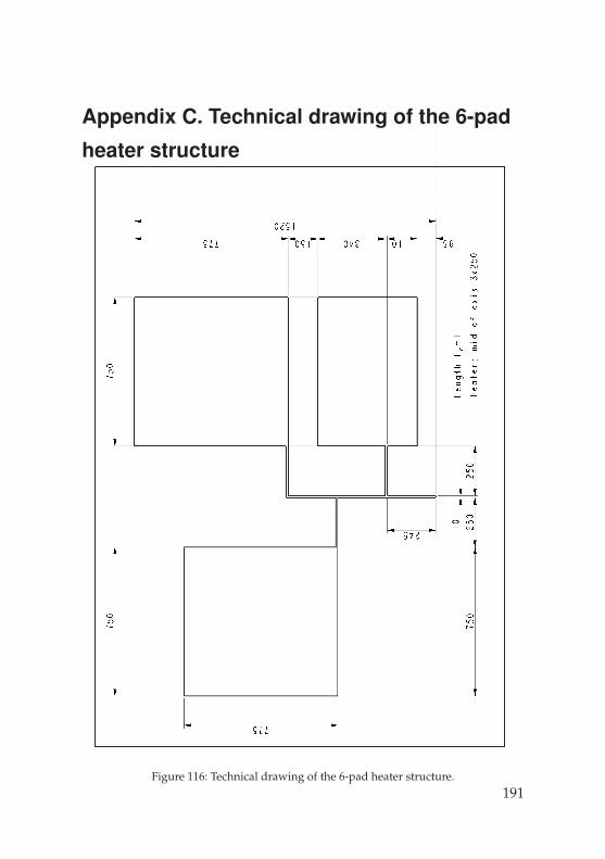
Appendix C. Technical drawing of the 6-pad
heater structure
Figure 116: Technical drawing of the 6-pad heater structure.191


Publications
S. Wiedigen, M. Feuchter, Ch. Jooss and M. Kamlah, 3-ωmeasurements of thermal conductivity in oxide thin films, poster at the‘DPG-conference’ in Regensburg, Germany (2010)
S. Wiedigen, M. Feuchter, M. Kamlah and Ch. Jooss, 3ωmeasurements of thermal conductivity in oxide thin films, oralpresentation at the ‘3 Omega workshop’ of the priority program inGottingen, Germany (2010)
M. Feuchter and M. Kamlah, Numerical analysis of the 3-ω-method formeasuring thermal conductivities in thermoelectric materials at thenanoscale, poster at the ‘HEAT conference’ in Erice, Italy (2010)
S. Wiedigen, M. Feuchter, Ch. Jooss and M. Kamlah, Understandingsize and interface dependent anisotropic thermal conduction in correlatedmultilayer structures, poster at the ‘status meeting of the priorityprogram’ in Berlin, Germany (2010)
S. Wiedigen, M. Feuchter, K. R. Mangipudi, Ch. Jooss, M. Kamlah,C. Volkert, Thermal conduction in correlated multilayer structures,poster at the ‘DPG-conference’ in Dresden, Germany (2011)
S. Wiedigen, T. Kramer, K. R. Mangipudi, M. Feuchter, Ch. Jooss, C.Volkert and M. Kamlah, Numerical analysis of the 3ω-method formeasuring thermal conductivities in thermoelectric materials at thenanoscale, poster at the ‘status meeting of the priority program’ inWittenberg, Germany (2011)
193

Publications
S. Wiedigen, T. Kramer, N. Folchert, J. Norpoth, Ch. Jooss, M.Feuchter, M. Kamlah, K. R. Mangipudi, C. A. Volkert, Thermalconductivity in correlated oxides, poster at the ‘status meeting of thepriority program’ in Wittenberg, Germany (2011)
M. Feuchter and M. Kamlah, Inverse Geometry configurations for the3ω-method, oral presentation at the ‘priority program summer school’in Cuxhaven, Germany (2011)
M. Feuchter and M. Kamlah, Numerical analysis of the 3ω-method, oralpresentation at the ‘COMSOL conference’ in Stuttgart, Germany(2011)
M. Feuchter and M. Kamlah, Numerical analysis of the 3ω-method, oralpresentation at the ‘Messtechnik workshop’ of the priority programin Kaub am Rhein, Germany (2012)
S. Wiedigen, T. Kramer, M. Feuchter K. R. Mangipudi, J. Hoffmann,M. Kamlah, C. A. Volkert and Ch. Jooss, Thermal conductivity inPr1−xCaxMnO3 and SrTiO3 thin film systems, poster at the ‘Messtechnikworkshop’ of the priority program in Kaub am Rhein, Germany(2012)
S. Wiedigen, T. Kramer, M. Feuchter, I. Knorr, N. Nee, J. Hoffmann,M. Kamlah, C. A. Volkert and Ch. Jooss, Interplay of point defects,biaxial strain, and thermal conductivity in homoepitaxial SrTiO3 thin films,Applied Physics Letters, 100 (2012), pp. 061904-4
194

Publications
M. Feuchter, S. Wiedigen, Ch. Jooss and M. Kamlah, A method todetermine the anisotropic thermal conduction of nanoscale thermoelectricmaterials by the use of multiphysical simulations and neural networks, oralpresentation at the ‘International Conference on ComputationalMethods ICCM’ in Gold Coast, Australia (2012)
M. Feuchter and M. Kamlah, Simulation of heat transfer in a3ω-measurement, oral presentation at the ‘Thermal Transport at theNanoscale’ workshop of the priority program in Bad Honnef,Germany (2013)
M. Feuchter and M. Kamlah, Simulation of heat transfer in a3ω-measurement, oral presentation at the ‘Germany/Japan Seminar onAdvanced Materials for Zero-Emission Energy’ workshop in Kyoto,Japan (2014)
195

References
[1] M. Abramowitz and I. A. Stegun, Handbook of mathematicalfunctions with formulas, graphs, and mathematical tables, U.S. Dept.of Commerce : U.S. G.P.O., Washington, D.C., (1972).
[2] S. Ahmed, R. Liske, T. Wunderer, M. Leonhardt, R. Ziervogel,C. Fansler, T. Grotjohn, J. Asmussen, and T. Schuelke,Extending the 3ω-method to the MHz range for thermal conductivitymeasurements of diamond thin films, Diamond and RelatedMaterials, 15 (2006), pp. 389–393.
[3] J. Alvarez-Quintana and J. Rodraguez-Viejo, Extension of the3ω method to measure the thermal conductivity of thin films withouta reference sample, Sensors and Actuators A: Physical, 142 (2008),pp. 232–236.
[4] S. P. Andersson and R. G. Ross, Thermal Conductivity and HeatCapacity per Unit Volume of Poly(methyl Methacrylate) Under HighPressure, International Journal of Thermophysics, 15, 5 (1994),pp. 949–962.
[5] G. Antonini, Internal impedance of conductors of rectangular crosssection, IEEE Transactions on Microwave Theory andTechniques, 47, 7 (1999), pp. 979–985.
[6] ASM International, Materials and Coatings for Medical Devices:Cardiovascular, ASM International, Materials Park, Ohio, (2009).
[7] A. Baikalov, Y. Q. Wang, B. Shen, B. Lorenz, S. Tsui, Y. Y. Sun,Y. Y. Xue, and C. W. Chu, Field-driven hysteretic and reversibleresistive switch at the Ag-Pr 0.7 Ca 0.3 MnO 3 interface, AppliedPhysics Letters, 83 (2003), pp. 957–959.
197
References
[8] H. Balke, Einfuhrung in die Technische Mechanik Festigkeitslehre,Springer-Verlag Berlin Heidelberg, Berlin, Heidelberg, (2010).
[9] H. Baltes, O. Brand, G. K. Fedder, C. Hierold, J. Korvink, and
O. Tabata, CMOS - MEMS; Advanced Micro & NanosystemsVolume 2, Wiley-VCH, (2005).
[10] G. M. Barrow and G. W. Herzog, Physikalische Chemie :Gesamtausgabe, Bohmann, Wien, (1984).
[11] H. Bateman, Tables of integral transforms Volume I., McGraw-HillBook Company INC., New York, N.Y., (1954).
[12] J.-L. Battaglia, C. Wiemer, and M. Fanciulli, An accuratelow-frequency model for the 3ω method, Journal of AppliedPhysics, 101 (2007), pp. 104510–5.
[13] T. Bergman, F. Incropera, A. Lavine, and D. DeWitt,Fundamentals of Heat and Mass Transfer, Wiley, (2011).
[14] R. P. Bhatta, S. Annamalai, R. K. Mohr, M. Brandys, I. L. Pegg,and B. Dutta, High temperature thermal conductivity of platinummicrowire by 3ω method, Review of Scientific Instruments, 81(2010), pp. 114904–5.
[15] H. H. Binder, Lexikon der chemischen Elemente : dasPeriodensystem in Fakten, Zahlen und Daten, S. Hirzel, Stuttgart,(1999).
[16] N. O. Birge, Specific-heat spectroscopy of glycerol and propyleneglycol near the glass transition, Physical Review B, 34 (1986),pp. 1631–1642.
198

References
[17] N. O. Birge and S. R. Nagel, Specific-heat spectroscopy of the glasstransition, Physical Review Letters, 54 (1985), pp. 2674–2677.
[18] O. Biro, P. Bohm, K. Preis, and G. Wachutka, Edge FiniteElement Analysis of Transient Skin Effect Problems, IEEETransactions on Magnetics, 36, 4 (2000), pp. 835–839.
[19] O. Biro and K. Preis, On the Use of the Magnetic Vector Votentialin the Finite Element Analysis of Three-Dimensional Eddy Currents,IEEE Transactions on Magnetics, 25 (1989), pp. 3145–3159.
[20] O. Biro, K. Preis, G. Buchgraber, and I. Ticar, Voltage-DrivenCoils in Finite-Element Formulations Using a Current Vector and aMagnetic Scalar Potential, IEEE Transactions on Magnetics, 40, 2(2004), pp. 1286–1289.
[21] P. Bockh, Warmeubertragung Grundlagen und Praxis,Springer-Verlag Berlin Heidelberg, Berlin, Heidelberg, (2006).
[22] T. Borca-Tasciuc, A. R. Kumar, and G. Chen, Data reduction in3ω method for thin-film thermal conductivity determination, Reviewof Scientific Instruments, 72 (2001), pp. 2139–2147.
[23] T. Borca-Tasciuc, D. W. Song, J. R. Meyer, I. Vurgaftman, M.-J.Yang, B. Z. Nosho, L. J. Whitman, H. Lee, R. U. Martinelli,G. W. Turner, M. J. Manfra, and G. Chen, Thermal conductivityof alas0.07sb0.93 and al0.9ga0.1as0.07sb0.93 alloys and(alas)1/(alsb)11 digital-alloy superlattices, Journal of AppliedPhysics, 92 (2002), pp. 4994–4998.
[24] T. Borca-Tasciuc, S. Vafaei, D.-A. Borca-Tasciuc, B. Q. Wei,R. Vajtai, and P. M. Ajayan, Anisotropic thermal diffusivity of
199
References
aligned multiwall carbon nanotube arrays, Journal of AppliedPhysics, 98 (2005), pp. 054309–6.
[25] A. I. Boukai, Y. Bunimovich, J. Tahir-Kheli, J.-K. Yu, W. A.Goddard III, and J. R. Heath, Silicon nanowires as efficientthermoelectric materials, Nature, 451 (2008), pp. 168–171.
[26] R. N. Bracewell, The Fourier Transform and Its Applications,McGraw-Hill Book Company INC., (2000).
[27] I. N. Bronstein, K. A. Semendjajew, G. Musiol, and H. Muhlig,Taschenbuch der Mathematik, Verlag Harri Deutsch, (2005).
[28] D. G. Cahill, Thermal conductivity measurement from 30 to 750 K:the 3ω method, Review of Scientific Instruments, 61 (1990),pp. 802–808.
[29] D. G. Cahill, Erratum: ”Thermal conductivity measurement from30 to 750 K: the 3ω method, Review of Scientific Instruments, 61(1990), pp. 802-808”, Review of Scientific Instruments, 73 (2002),pp. 3701–3701.
[30] D. G. Cahill and T. H. Allen, Thermal conductivity of sputteredand evaporated SiO2 and TiO2 optical coatings, Applied PhysicsLetters, 65 (1994), pp. 309–311.
[31] D. G. Cahill, W. K. Ford, K. E. Goodson, G. D. Mahan,A. Majumdar, H. J. Maris, R. Merlin, and S. R. Phillpot,Nanoscale thermal transport, Journal of Applied Physics, 93(2003), pp. 793–818.
[32] D. G. Cahill, M. Katiyar, and J. R. Abelson, Thermalconductivity of a-Si:H thin films, Physical Review B, 50 (1994),pp. 6077–6081.
200

References
[33] D. G. Cahill, S.-M. Lee, and T. I. Selinder, Thermal conductivityof κ-Al2O3 and α-Al2O3 wear-resistant coatings, Journal ofApplied Physics, 83 (1998), pp. 5783–5786.
[34] D. G. Cahill and R. O. Pohl, Thermal conductivity of amorphoussolids above the plateau, Physical Review B, 35 (1987),pp. 4067–4073.
[35] H. S. Carslaw and J. C. Jaeger, Conduction of heat in solids,Second Edition, Clarendon Press - Oxford, (1959).
[36] W.-Y. Chang, J.-H. Liao, Y.-S. Lo, and T.-B. Wu, Resistiveswitching characteristics in Pr0.7Ca0.3MnO3 thin films onLaNiO3-electrodized Si substrate, Applied Physics Letters, 94(2009), pp. 172107–3.
[37] C.-P. Chen and C. Mortici, New sequence converging towards theEuler-Mascheroni constant, Computers and Mathematics withApplications, 64 (2012), pp. 391–398.
[38] F. Chen, J. Shulman, Y. Xue, C. W. Chu, and G. S. Nolas,Thermal conductivity measurement under hydrostatic pressure usingthe 3ω method, Review of Scientific Instruments, 75 (2004),pp. 4578–4584.
[39] Y. Chen, W. Tian, H. Li, X. Wang, and W. Zhu, PCMO DeviceWith High Switching Stability, IEEE Electron Device Letters, 31(2010), pp. 866–868.
[40] S. R. Choi, J. Kim, and D. Kim, 3ω method to measure thermalproperties of electrically conducting small-volume liquid, Review ofScientific Instruments, 78 (2007), pp. 084902–6.
201

References
[41] H. M. Christen, E. D. Specht, S. S. Silliman, and K. S.Harshavardhan, Ferroelectric and antiferroelectric coupling insuperlattices of paraelectric perovskites at room temperature,Physical Review B, 68 (2003), p. 020101.
[42] W.-H. Chuang, T. Luger, R. K. Fettig, and R. Ghodssi,Mechanical Property Characterization of LPCVD Silicon NitrideThin Films at Cryogenic Temperatures, Journal ofMicroelectromechanical Systems, 13 (5) (2004), pp. 870–879.
[43] B. T. Cong, T. Tsuji, P. X. Thao, P. Q. Thanh, and Y. Yamamura,High-temperature thermoelectric properties of Ca1−xPrxMnO3−δ(0 ≤x < 1), Physica B: Condensed Matter, 352 (2004), pp. 18–23.
[44] O. Corbino, Periodische Widerstandsanderungen von Metallfaden.,Physikalische Zeitschrift, 12 (1911), pp. 292–295.
[45] crystec. http://www.crystec.de/ daten/ srtio3.pdf, (03:20 p.m.,14 Jun.2013).
[46] P. Csıkvari, P.Furjes, C. Ducso, and I. Barsony, Micro-hotplatesfor thermal characterisation of structural materials of MEMS,Microelectronics Journal, 40 (2009), pp. 1393–1397.
[47] C. Dames and G. Chen, 1ω, 2ω, and 3ω methods for measurementsof thermal properties, Review of Scientific Instruments, 76 (2005),pp. 124902–14.
[48] A. Daoud-Aladine, J. Rodrguez-Carvajal,L. Pinsard-Gaudart, M. T. Fernndez-Daz, and
A. Revcolevschi, Zener Polaron Ordering in Half-DopedManganites, Physical Review Letters, 89 (2002), p. 097205.
202

References
[49] N. Das, S. Tsui, Y. Y. Xue, Y. Q. Wang, and C. W. Chu,Electric-field-induced submicrosecond resistive switching, PhysicalReview B, 78 (2008), pp. 235418–.
[50] R. M. Dreizler and C. S. Ludde, Theoretische Physik 2 -Elektrodynamik und spezielle Relativitatstheorie, Springer-VerlagBerlin Heidelberg, Berlin, Heidelberg, (2005).
[51] A. Duran, F. Morales, L. Fuentes, and J. M. Siqueiros, Specificheat anomalies at 37, 105 and 455 K in SrTiO3 : Pr, Journal ofPhysics: Condensed Matter, 20 (2008), p. 085219.
[52] S. N. Dyer, Survey of instrumentation and measurement,Wiley-Interscience, John Wiley and Sons, Inc., New York, (2001).
[53] D. V. Efremov, J. van den Brink, and D. I. Khomskii, Chargeorder versus Zener polarons: ferroelectricity in manganites,Condensed Matter, 1 (2003), p. 0306651.
[54] D. V. Efremov, J. van den Brink, and D. I. Khomskii, Bond-versus site-centred ordering and possible ferroelectricity inmanganites, Nature Materials, 3 (2004), pp. 853–856.
[55] electric ray. http://electric-ray.com/ Tesla Roadster cutaway.jpg,(10:06 a.m., 23 Jan. 2013).
[56] R. Farraro and R. Mclellan, Temperature Dependence of theYoung’s Modulus and Shear Modulus of Pure Nickel, Platinum, andMolybdenum, Metallurgical Transactions A, 8 (1977),pp. 1563–1565.
[57] R. P. Feynman, Lectures on Physics, Addison-Wesley Pub. Co.,(1963).
203

References
[58] H. Ftouni, C. Blanc, A. Sikora, J. Richard, M. Defoort,K. Lulla, E. Collin, and O. Bourgeois, Thermal conductivitymeasurement of suspended Si-N membranes from 10 K to 275 Kusing the 3ω-Volklein method, Journal of Physics: ConferenceSeries, 395 (2012), p. 012109.
[59] M. Fujimoto, H. Koyama, Y. Nishi, and T. Suzuki, Resistiveswitching properties of high crystallinity and low-resistancePr0.7Ca0.3MnO3 thin film with point-contacted Ag electrodes,Applied Physics Letters, 91 (2007).
[60] R. Gasch, K. Knothe, and R. Liebich, Strukturdynamik - DiskreteSysteme und Kontinua, Springer-Verlag Berlin Heidelberg,(2012).
[61] A. K. Gasiorski, A finite element method for analysing skin effect inconductors with unknown values of surface boundary conditions,International Journal for Numerical Methods in Engineering, 21(1985), pp. 1641–1657.
[62] H. Gercek, Poisson’s ratio values for rocks, International Journalof Rock Mechanics and Mining Sciences, 44 (2007), pp. 1–13.
[63] C. Gerthsen, H. O. Kneser, and H. Vogel, Physik,Springer-Verlag Berlin Heidelberg New York, (1974).
[64] M. Greconici, G. Madescu, and M. Mot, Skin Effect Analysis ina Free Space Conductor, SER.: ELEC. ENERG., 23, 2 (2010),pp. 207–215.
[65] greencar. http://cdn-www.greencar.com/ images/ waste- exhaust-heat- generates- electricity- cars- efficient.php/ bmw-teg-1.jpg, (10:08a.m., 23 Jan. 2013).
204

References
[66] D. J. Griffiths, Introduction to Electrodynamics, Prentice-Hall,Upper Saddle River, N.J., (1999).
[67] D. Gross, W. Hauger, and P. Wriggers, Technische Mechanik 4,Springer, Berlin; Heidelberg, (2009).
[68] D. Gross and T. Seelig, Bruchmechanik - Mit einer Einfuhrung indie Mikromechanik, Springer-Verlag, Berlin; New York, (2006).
[69] S. P. Gurrum, W. P. King, and Y. K. Joshi, A semianalyticalsolution for the 3ω method including the effect of heater thermalconduction, Journal of Applied Physics, 103 (2008), pp. 113517–6.
[70] L. D. Hicks and M. S. Dresselhaus, Effect of quantum-wellstructures on the thermoelectric figure of merit, Physical Review B,47 (1993), pp. 12727–12731.
[71] C. Y. Ho, R. W. Powell, and P. E. Liley, Thermal Conductivity ofthe Elements, Journal of Physical and Chemical Reference Data,1 (1972), p. 279.
[72] E. A. Hoffmann, H. A. Nilsson, J. E. Matthews,N. Nakpathomkun, A. I. Persson, L. Samuelson, and H. Linke,Measuring Temperature Gradients over Nanometer Length Scales,Nano Letters, 9 (2009), pp. 779–783.
[73] N. Huber, Anwendung Neuronaler Netze bei nichtlinearenProblemen der Mechnaik, FZKA 6504, (2000).
[74] R. E. Hummel, Electronic Properties of Materials, Springer, NewYork, (2005).
205
References
[75] International Energy Agency, World energy outlook 2012 -executive summary, http://www.worldenergyoutlook.org/,(2012).
[76] J. D. Jackson, Klassische Elektrodynamik, Walter de Gruyter,Berlin, (1982).
[77] A. Jacquot, G. Chen, H. Scherrer, A. Dauscher, and B. Lenoir,Improvements of on-membrane method for thin film thermalconductivity and emissivity measurements, Sensors and ActuatorsA: Physical, 117 (2005), pp. 203–210.
[78] A. Jacquot, B. Lenoir, A. Dauscher, M. Stolzer, and J. Meusel,Numerical simulation of the 3ω method for measuring the thermalconductivity, Journal of Applied Physics, 91 (2002),pp. 4733–4738.
[79] A. Jacquot, F. Vollmer, B. Bayer, M. Jaegle, D. Ebling, and
H. Boettner, Thermal Conductivity Measurements on ChallengingSamples by the 3 Omega Method, Journal of Electronic Materials,39 (2010), pp. 1621–1626.
[80] T. Jaeger, Thermoelectric properties of TiNiSn and Zr0.5Hf0.5NiSnthin films and superlattices with reduced thermal conductivities,Ph.D.-thesis, Johannes Gutenberg-Universitat, Mainz,Germany, (2013).
[81] T. Jaeger, C. Mix, M. Schwall, X. Kozina, J. Barth, B. Balke,M. Finsterbusch, Y. U. Idzerda, C. Felser, and G. Jakob,Epitaxial growth and thermoelectric properties of TiNiSn andZr0.5Hf0.5NiSn thin films, Thin Solid Films, 520 (2011),pp. 1010–1014.
206

References
[82] A. Jain and K. E. Goodson, Measurement of the ThermalConductivity and Heat Capacity of Freestanding Shape Memory ThinFilms Using the 3ω Method, Journal of Heat Transfer, 130 (2008),pp. 102402–7.
[83] K. Jakubiuk and P. Zimny, Skin effect in rectangular conductors,Journal of Physics A: Mathematical and General, 9, 4 (1976),pp. 669–676.
[84] R. Jenisch and M. Stohrer, Warme, in Lehrbuch der Bauphysik,Vieweg+Teubner, (2008), pp. 107–335.
[85] C. Jooss, L.Wu, T. Beetz, R. F. Klie, M. Beleggia, M. A.Schofield, S. Schramm, J. Hoffmann, and Y. Zhu, Polaronmelting and ordering as key mechanisms for colossal resistance effectsin manganites, Proceedings of the National Academy of Science,104 (2007), pp. 13597–13602.
[86] M. Kamlah, Zur Modellierung des Verfestigungsverhaltens vonMaterialien mit statischer Hysterese im Rahmen derphanomenologischen Thermomechanik, PhD thesis, UniversitatGesamthochschule Kassel, (1994).
[87] R. Karthik, R. Harish Nagarajan, B. Raja, and
P. Damodharan, Thermal conductivity of CuO-DI water nanofluidsusing 3-ω measurement technique in a suspended micro-wire,Experimental Thermal and Fluid Science, xx (2012), pp. –.
[88] S. P. Keane, S. Schmidt, J. Lu, A. E. Romanov, and S. Stemmer,Phase transitions in textured SrTiO3 thin films on epitaxial Ptelectrodes, Journal of Applied Physics, 99 (2006), p. 033521.
207

References
[89] C. J. Kim and I.-W. Chen, Effect of top electrode on resistanceswitching of (Pr,Ca)MnO3 thin films, Thin Solid Films, 515 (2006),pp. 2726–2729.
[90] D. S. Kim, Y. H. Kim, C. E. Lee, and Y. T. Kim, Colossalelectroresistance mechanism in a Au/Pr0.7Ca0.3MnO3/pt sandwichstructure: Evidence for a Mott transition, Physical Review B, 74(2006), p. 174430.
[91] J. H. Kim, A. Feldman, and D. Novotny, Application of the threeomega thermal conductivity measurement method to a film on asubstrate of finite thickness, Journal of Applied Physics, 86 (1999),pp. 3959–3963.
[92] R. K. Kirby, Platinum - A Thermal Expansion Reference Material,International Journal of Thermophysics, 12 , 4 (1991).
[93] K. Knothe and H. Wessels, Finite Elemente - Eine Einfuhrung furIngenieure, Springer-Verlag Berlin Heidelberg, (2008).
[94] korth. http://www.korth.de/ index.php/ material- detailansicht/items/22.html, (05.04 p.m.,14. Jun. 2013).
[95] K. Koumoto, Y. Wang, R. Zhang, A. Kosuga, and R. Funahashi,Oxide Thermoelectric Materials: A Nanostructuring Approach,Annual Review of Materials Research, 40 (2010), pp. 363–394.
[96] R. Kruse, Computational Intelligence : Eine methodischeEinfuhrung in Kunstliche Neuronale Netze, EvolutionareAlgorithmen, Fuzzy-Systeme und Bayes-Netze; 43 Tab., Vieweg +
Teubner, Wiesbaden, (2011).
208

References
[97] K. Kurosaki, D. Setoyama, J. Matsunaga, and S. Yamanaka,Nanoindentation tests for TiO2, MgO, and YSZ single crystals,Journal of Alloys and Compounds, 386 (2005), pp. 261–264.
[98] M. Leclerc and A. Najari, Organic thermoelectrics: Green energyfrom a blue polymer, Nature Materials, 10 (2011), pp. 409–410.
[99] S.-M. Lee and D. G. Cahill, Heat transport in thin dielectric films,Journal of Applied Physics, 81 (1997), pp. 2590–2595.
[100] S.-M. Lee, D. G. Cahill, and T. H. Allen, Thermal conductivity ofsputtered oxide films, Physical Review B, 52 (1995), pp. 253–257.
[101] S.-M. Lee, D. G. Cahill, and R. Venkatasubramanian, Thermalconductivity of Si-Ge superlattices, Applied Physics Letters, 70(1997), pp. 2957–2959.
[102] M. R. Lees, O. A. Petrenko, G. Balakrishnan, and D. McK.Paul, Specific heat of Pr0.6(Ca1−xSrx)0.4MnO3 (0 ≤ x ≤ 1), PhysicalReview B, 59 (2) (1999), pp. 1298–1303.
[103] P. Leonard and D. Rodger, Finite element scheme for transient 3Deddy currents, IEEE Transactions on Magnetics, 24 (1988),pp. 90–93.
[104] S.-L. Li, D. S. Shang, J. Li, J. L. Gang, and D. N. Zheng, Resistiveswitching properties in oxygen-deficient Pr0.7Ca0.3MnO3 junctionswith active Al top electrodes, Journal of Applied Physics, 105(2009).
[105] Z. L. Liao, Z. Z. Wang, Y. Meng, Z. Y. Liu, P. Gao, J. L. Gang,H. W. Zhao, X. J. Liang, X. D. Bai, and D. M. Chen,Categorization of resistive switching of
209
References
metal-Pr0.7Ca0.3MnO3-metal devices, Applied Physics Letters, 94(2009).
[106] D. R. Lide, CRC Handbook of Chemistry and Physics, CRC Press,Boca Raton, Florida, Boca Raton, Fla., (2009).
[107] M. E. Lines and A. M. Glass, Principles and Applications ofFerroelectrics and Related Materials, Clarendon Press - Oxford,Oxford, (1977).
[108] S. Q. Liu, N. J. Wu, and A. Ignatiev, Electric-pulse-inducedreversible resistance change effect in magnetoresistive films, AppliedPhysics Letters, 76 (2000), pp. 2749–2751.
[109] W. Liu, Y. Yang, and M. Asheghi, Thermal and electricalcharacterization and modeling of thin copper layers, ITHERM ’06.The Tenth Intersociety Conference, (2006), pp. 1171–1176.
[110] L. Lu, W. Yi, and D. L. Zhang, 3ω method for specific heat andthermal conductivity measurements, Review of ScientificInstruments, 72 (2001), pp. 2996–3003.
[111] J. Lunze, Regelungstechnik 1, Springer-Verlag Berlin Heidelberg,(2007).
[112] H. M.A., N. W.D., and K. T.W., What is the Young’s Modulus ofSilicon?, Journal of Microelectromechanical Systems, 19, 2(2010), pp. 229–238.
[113] L. E. Malvern, Introduction to the mechanics of a continuousmedium, Prentice-Hall, Inc., Englewood Cliffs, N.J., (1969).
210

References
[114] C. H. Mastrangelo, Y.-C. Tai, and R. S. Muller, Thermophysicalproperties of low-residual stress, Silicon-rich, LPCVD silicon nitridefilms, Sensors and Actuators A: Physical, 23 (1990), pp. 856–860.
[115] J. C. Maxwell, A Dynamical Theory of the Electromagnetic Field,Philosophical Transactions of the Royal Society of London, 155(1865), pp. 459–512.
[116] T. E. Mitchell, Dislocations and Mechanical Properties ofMgO-Al2O3 Spinel Single Crystals, Journal of the AmericanCeramic Society, 82 (12) (1999), pp. 3305–3316.
[117] I. K. Moon, Y. H. Jeong, and S. I. Kwun, The 3ω technique formeasuring dynamic specific heat and thermal conductivity of a liquidor solid, Review of Scientific Instruments, 67 (1996), pp. 29–35.
[118] R. E. Moritz, Memorabilia mathematica; or, The philomath’squotation-book., The Macmillan Company, (1914).
[119] n tv. http://bilder3.n-tv.de/ img/ incoming/ origs6923101/
3272734610- w1000- h960/ curiosity2.jpg, (09:45 a.m., 23 Jan.2013).
[120] C. Nauenheim, C. Kugeler, A. Rudiger, R. Waser, A. Flocke,and T. Noll, Nano-Crossbar Arrays for Nonvolatile Resistive RAM(RRAM) Applications, NANO’08. 8th IEEE conference onNanotechnology, (2008), pp. 464–467.
[121] ndtguide. http://ndtguide.com/ wiki/ mp/ Permeability.pdf, (10:43a.m., 14 Jun. 2013).
[122] K. Nielsch, J. Bachmann, J. Kimling, and H. Bttner,Thermoelectric Nanostructures: From Physical Model Systems
211

References
towards Nanograined Composites, Advanced Energy Materials, 1(2011), pp. 713–731.
[123] Y. Nomura, R. Horlein, P. Tzallas, B. Dromey, S. Rykovanov,Z. Major, J. Osterhoff, S. Karsch, L. Veisz, M. Zepf,D. Charalambidis, F. Krausz, and G. D. Tsakiris, Attosecondphase locking of harmonics emitted from laser-produced plasmas,Nature Physics, 5 (2009), pp. 124–128.
[124] D.-W. Oh, A. Jain, J. K. Eaton, K. E. Goodson, and J. S. Lee,Thermal conductivity measurement and sedimentation detection ofaluminum oxide nanofluids by using the 3ω method, InternationalJournal of Heat and Fluid Flow, 29 (2008), pp. 1456–1461.
[125] H. Ohta, S. Kim, Y. Mune, T. Mizoguchi, K. Nomura, S. Ohta,T. Nomura, Y. Nakanishi, Y. Ikuhara, M. Hirano, H. Hosono,and K. Koumoto, Giant thermoelectric Seebeck coefficient of atwo-dimensional electron gas in SrTiO3, Nature Materials, 6(2007), pp. 129–134.
[126] B. W. Olson, S. Graham, and K. Chen, A practical extension ofthe 3ω method to multilayer structures, Review of ScientificInstruments, 76 (2005), pp. 053901–7.
[127] B. K. Park, J. Park, and D. Kim, Note: Three-omega method tomeasure thermal properties of subnanoliter liquid samples, Review ofScientific Instruments, 81 (2010), pp. 066104–3.
[128] M. Paz and W. Leigh, Structural Dynamics - Theory andComputation, Kluwer Academic, (2004).
212

References
[129] P. Pichanusakorn and P. Bandaru, Nanostructuredthermoelectrics, Materials Science and Engineering: R: Reports,67 (2010), pp. 19–63.
[130] Z. B. Popovic and B. D. Popovic, Introductory Electromagnetics,Addison-Wesley Pub. Co., (1999).
[131] B. Poudel, Q. Hao, Y. Ma, Y. Lan, A. Minnich, B. Yu, X. Yan,D. Wang, A. Muto, D. Vashaee, X. Chen, J. Liu, M. S.Dresselhaus, G. Chen, and Z. Ren, High-ThermoelectricPerformance of Nanostructured Bismuth Antimony Telluride BulkAlloys, Science, 320 (2008), pp. 634–638.
[132] S. S. Rao, The Finite Element Method in Engineering,Butterworth-Heinemann, imprint of Elsevier, (2011).
[133] C. E. Raudzis, Anwendung und Erweiterung der 3ω Methode zurCharakterisierung komplexer Mehrschichtsysteme in derMikrosystemtechnik, Der Andere Verlag, Tonning LubeckMarburg, (2007).
[134] C. E. Raudzis, F. Schatz, and D. Wharam, Extending the 3ωmethod for thin-film analysis to high frequencies, Journal ofApplied Physics, 93 (2003), pp. 6050–6055.
[135] raumfahrer. http://www.raumfahrer.net/ news/ images/orion esa sm1.jpg, (10:26 a.m., 23 Jan. 2013).
[136] S.-C. Roh, Y.-M. Choi, and S.-Y. Kim, Sensitivity enhancement of asilicon micro-machined thermal flow sensor, Sensors and ActuatorsA: Physical, 128 (2006), pp. 1–6.
[137] D. Rowe, CRC Handbook of Thermoelectrics, CRC Press, BocaRaton, (1995).
213
References
[138] D. M. Rowe and C. M. Bhandari, Modern Thermoelectrics,Reston Publishing Company, Inc., (1983).
[139] A. Salvatore, Finite-Element Mesh Adaptation of 2-DTime-Harmonic Skin Effect Problems, IEEE Transactions onMagnetics, 36, 4 (2000), pp. 1592–1595.
[140] S. Scherrer-Rudiy, Bewertung von Unsicherheiten beiwerkstoffmechanischen Fragestellungen mit dem Bayes-Verfahren,PhD thesis, Forschungszentrum Karlsruhe, FZKA 7491, (2009).
[141] H. Schubert, Anisotropic Thermal Expansion Coefficients ofY2O3-Stabilized Tetragonal Zirconia, Journal of the AmericanCeramic Society, 69, 3 (1986), pp. 270–271.
[142] T. J. Seebeck, Magnetische Polarisation der Metalle und Erze durchTemperatur-Differenz. (1822-1823), A. J. v. Oettingen, Verlag vonWilhelm Engelmann, (1895).
[143] S. Shafiee and E. Topal, An econometrics view of worldwide fossilfuel consumption and the role of US, Energy Policy, 36 (2008),pp. 775–786.
[144] S. Shin, H. N. Cho, B. S. Kim, and H. H. Cho, Influence of upperlayer on measuring thermal conductivity of multilayer thin filmsusing differential 3-ω method, Thin Solid Films, 517 (2008),pp. 933–936.
[145] G. J. Snyder and E. S. Toberer, Complex thermoelectric materials,Nature Materials, 7 (2008), pp. 105–114.
[146] Q. Song, Z. Cui, S. Xia, Z. Chen, and J. Zhang, Measurement ofSiNx thin film thermal property with suspended membrane structure,Sensors and Actuators A: Physical, 112 (2004), pp. 122–126.
214
References
[147] X. Song, M. Xie, F. Zhou, G. Jia, X. Hao, and S. An,High-temperature thermal properties of yttria fully stabilized zirconiaceramics, Journal of Rare Earths, 29 (2011), pp. 155–159.
[148] A. Stranz, U. Sokmen, J. Kahler, A. Waag, and E. Peiner,Measurements of thermoelectric properties of silicon pillars, Sensorsand Actuators A: Physical, 171 (2011), pp. 48–53.
[149] T. R. Taylor, P. J. Hansen, B. Acikel, N. Pervez, R. A. York,S. K. Streiffer, and J. S. Speck, Impact of thermal strain on thedielectric constant of sputtered barium strontium titanate thin films,Applied Physics Letters, 80 (2002), pp. 1978–1980.
[150] thermoelectric. http://www.thermoelectric.com/ 2005/ images/te.jpg, (11.20 a.m., 09. Aug. 2012).
[151] R. J. D. Tilley, Understanding Soilds - The Science of Materials,John Wiley and Sons, Inc., (2004).
[152] T. Tong and A. Majumdar, Reexamining the 3-omega technique forthin film thermal characterization, Review of ScientificInstruments, 77 (2006), pp. 104902–9.
[153] tuvie. http://www.tuvie.com/ wp-content/ uploads/ Orange- power-whellies2.jpg, (09:54 a.m., 23 Jan. 2013).
[154] E. Tyulyukovskiy and N. Huber, Identificationof visco plasticmaterial parameters from spherical identation data. Part I: Neuralnetworks, Journal of Materials Research, 21 (2006), pp. 664–676.
[155] J. van den Brink and D. I. Khomskii, Multiferroicity due to chargeordering, Journal of Physics: Condensed Matter, 20 (2008),p. 434217.
215

References
[156] R. Venkatasubramanian, Lattice thermal conductivity reductionand phonon localizationlike behavior in superlattice structures,Physical Review B, 61 (2000), pp. 3091–3097.
[157] R. Venkatasubramanian, E. Siivola, T. Colpitts, and
B. O’Quinn, Thin-film thermoelectric devices with highroom-temperature figures of merit, Nature, 413 (2001), pp. 597–602.
[158] C. B. Vining, An inconvenient truth about thermoelectrics, NatureMaterials, 8 (2009), pp. 83–85.
[159] F. Volklein, Thermal conductivity and diffusivity of a thin filmSiO2 − Si3N4 sandwich system, Thin Solid Films, 188 (1990),pp. 27–33.
[160] A. Wahl, V. Hardy, C. Martin, and C. Simon, Magneticcontributions to the low-temperature specific heat of the ferromagneticinsulator Pr0.8Ca0.2MnO3, The European Physical Journal B, 26(2002), pp. 135–140.
[161] H. Wang and M. Sen, Analysis of the 3-omega method for thermalconductivity measurement, International Journal of Heat andMass Transfer, 52 (2009), pp. 2102–2109.
[162] X. Wang and P. Xiao, Residual stresses and constrained sintering ofYSZ/Al2O3 composite coatings, Acta Materialia, 52 (2004),pp. 2591–2603.
[163] Z. L. Wang, D. W. Tang, and X. H. Zheng, Simultaneousdetermination of thermal conductivities of thin film and substrate byextending 3ω-method to wide-frequency range, Applied SurfaceScience, 253 (2007), pp. 9024–9029.
216
References
[164] S. Wiedigen, T. Kramer, M. Feuchter, I. Knorr, N. Nee,J. Hoffmann, M. Kamlah, C. A. Volkert, and C. Jooss, Interplayof point defects, biaxial strain, and thermal conductivity inhomoepitaxial srtio3 thin films, Applied Physics Letters, 100(2012), pp. 061904–4.
[165] W. Xu, J. Li, G. Zhang, X. Chen, R. Galos, H. Hadim, M. Lu,and Y. Shi, A low-cost MEMS tester for measuring singlenanostructure’s thermal conductivity, Sensors and Actuators A:Physical, 191 (2013), pp. 89–98.
[166] Y. Xu, Z. Shi, C. Guo, and J. Zhao, Analysis of key stresses ofcoated tool in high speed cutting, Applied Mechanics andMaterials, 151 (2012), pp. 442–445.
[167] J. Yu, Z. Tang, F. Zhang, H. Ding, and Z. Huang, Measurementof the Heat Capacity of Copper Thin Films Using a MicropulseCalorimeter, Journal of Heat Transfer, 132 (2010),pp. 012403–012406.
[168] J.-K. Yu, S. Mitrovic, D. Tham, J. Varghese, and J. R. Heath,Reduction of thermal conductivity in phononic nanomesh structures,Nature Nanotechnology, 5 (2010), pp. 718–721.
[169] E. Yusibani, P. Woodfield, M. Fujii, K. Shinzato, X. Zhang, and
Y. Takata, Application of the Three-Omega Method to Measurementof Thermal Conductivity and Thermal Diffusivity of Hydrogen Gas,International Journal of Thermophysics, 30 (2009), pp. 397–415.
[170] J. Zhang, A. A. Heitmann, S. P. Alpay, and G. A. Rossetti Jr.,Electrothermal properties of perovskite ferroelectric films, Journal ofMaterial Science, 44 (2009), pp. 5263–5273.
217

References
[171] K. L. Zhang, S. K. Chou, and S. S. Ang, Performance Prediction ofa Novel Solid-Propellant Microthruster, Journal of Propulsion andPower, 22, 1 (2006).
[172] B. Zheng, Z. Xiao, B. Chhay, R. Zimmerman, M. E. Edwards,and D. ILA, Thermoelectric properties of MeV Si ion bombardedBi2Te3/Sb2Te3 superlattice deposited by magnetron sputtering,Surface and Coatings Technology, 203 (2009), pp. 2682–2686.
[173] Z.-X. Zong, Z.-J. Qiu, S.-L. Zhang, R. Streiter, and R. Liu, Ageneralized 3ω method for extraction of thermal conductivity in thinfilms, Journal of Applied Physics, 109 (2011), pp. 063502–8.
218


Acknowledgment - Danksagung
Die vorliegende Arbeit wurde im Teilinstitut Werkstoff- undBiomechanik (WBM) des Instituts fur Angewandte Materialien (IAM)am Karlsruher Institut fur Technologie (KIT) im Zeitraum vonOktober 2009 bis Mai 2014 angefertigt.
Zu Beginn mochte ich meinem Betreuer Herrn Prof. Dr. MarcKamlah außerordentlich danken. Nur durch seine fachlich sehrkompetente Betreuung und zahlreichen Hilfestellungen beimultiphysikalischen Fragen war es mir moglich das benotigteVerstandnis zu entwickeln und diese Arbeit anzufertigen. Ich dankeihm auch sehr fur ein freundschaftliches Arbeitsklima, bei dem mansich unter viel Freiraum trotzdem stets gefordert fuhlt.
Meinen Kooperations- und Projektpartnern aus Clausthal undGottingen danke ich fur viele interessante Arbeitstreffen. Vor allemden Arbeitsgruppen von Prof. Dr. Christian Jooss und Prof. Dr.Cynthia Volkert danke ich fur die vielen Fragestellungen undAnregungen. Im Besonderen mochte ich auch Stefanie Wiedigen,Thilo Kramer und Malte Scherff fur die experimentellen Messungendieser Arbeit sowie hilfreichen Diskussionen danken. Daruberhinaus geht ein spezieller Dank an Herrn Prof. Dr. Volklein. Er berietmich nicht nur mit jahrelangem Fachwissen zu Membransystemensondern stellte mir auch thermische und mechanische Materialdatenzur Verfugung.
221

Ebenso mochte ich Prof. Kamlah fur die Ubernahme desHauptreferats sowie Prof. Jooss fur die Ubernahme des erstenKorreferats danken. Herrn Prof. Dr. Oliver Kraft danke ich fur dieAufnahme an seinem Institut und die Ubernahme des zweitenKorreferats.
Auch bei Dr. Ingo Munch mochte ich mich bedanken. Er wecke beimir das Interesse fur wissenschaftliches Arbeiten wahrend meinerDiplomarbeit und fuhrte mich in das interessante Feld dermultiphysikalischen Simulationen ein. Ebenso gilt mein Dank HerrnProf. Dr. Werner Wagner. Durch seine Studiums begleitendeBetreuung als Mentor war es mir moglich einen englischsprachigenAuslandsaufenthalt zu absolvieren und dabei vor allem meineEnglischkenntnisse zu erwerben.
Ich danke allen Kollegen fur zahlreiche fachliche Diskussionen undeine wunderbare Arbeitsatmosphare in den letzten Jahren. So mochteich auch im Speziellen der Arbeitsgruppe von Prof. Kamlah, sowiemeinen langjahrigen Zimmerkollegen danken. Daruber hinausbedanke ich mich bei Frau Dr. Svetlana Scherrer-Rudiy fur dieEinuhrung in die Parameteridentifikation mittels Neuronaler Netze.Ebenso gilt mein Dank Matthew Berwind fur das Lektorieren dieserin Englisch geschriebenen Arbeit.
Am Ende mochte ich mich ganz herzlich bei meinen Eltern Angelikaund Klaus, meinem Bruder Julius, sowie meiner Freundin Evelyn, furjegliche Unterstutzung und Motivation auf meinem bisherigenLebensweg bedanken.
Manuel Feuchter, Fruhjahr 2014
222


Band 1 Prachai Norajitra Divertor Development for a Future Fusion Power Plant. 2011 ISBN 978-3-86644-738-7
Band 2 Jürgen Prokop Entwicklung von Spritzgießsonderverfahren zur Herstellung von Mikrobauteilen durch galvanische Replikation. 2011 ISBN 978-3-86644-755-4
Band 3 Theo Fett New contributions to R-curves and bridging stresses – Applications of weight functions. 2012 ISBN 978-3-86644-836-0
Band 4 Jérôme Acker Einfluss des Alkali/Niob-Verhältnisses und der Kupferdotierung auf das Sinterverhalten, die Strukturbildung und die Mikro - struktur von bleifreier Piezokeramik (K0,5Na0,5)NbO3. 2012 ISBN 978-3-86644-867-4
Band 5 Holger Schwaab Nichtlineare Modellierung von Ferroelektrika unter Berücksichtigung der elektrischen Leitfähigkeit. 2012 ISBN 978-3-86644-869-8
Band 6 Christian Dethloff Modeling of Helium Bubble Nucleation and Growth in Neutron Irradiated RAFM Steels. 2012 ISBN 978-3-86644-901-5
Band 7 Jens Reiser Duktilisierung von Wolfram. Synthese, Analyse und Charak teri sierung von Wolframlaminaten aus Wolframfolie. 2012 ISBN 978-3-86644-902-2
Band 8 Andreas Sedlmayr Experimental Investigations of Deformation Pathways in Nanowires. 2012 ISBN 978-3-86644-905-3
Schriftenreihedes Instituts für Angewandte Materialien
ISSN 2192-9963
Die Bände sind unter www.ksp.kit.edu als PDF frei verfügbar oder als Druckausgabe bestellbar.

Band 9 Matthias Friedrich Funk Microstructural stability of nanostructured fcc metals during cyclic deformation and fatigue. 2012 ISBN 978-3-86644-918-3
Band 10 Maximilian Schwenk Entwicklung und Validierung eines numerischen Simulationsmodells zur Beschreibung der induktiven Ein- und Zweifrequenz randschicht - härtung am Beispiel von vergütetem 42CrMo4. 2012 ISBN 978-3-86644-929-9
Band 11 Matthias Merzkirch Verformungs- und Schädigungsverhalten der verbundstrang gepressten, federstahldrahtverstärkten Aluminiumlegierung EN AW-6082. 2012 ISBN 978-3-86644-933-6
Band 12 Thilo Hammers Wärmebehandlung und Recken von verbundstranggepressten Luftfahrtprofilen. 2013 ISBN 978-3-86644-947-3
Band 13 Jochen Lohmiller Investigation of deformation mechanisms in nanocrystalline
metals and alloys by in situ synchrotron X-ray diffraction. 2013 ISBN 978-3-86644-962-6
Band 14 Simone Schreijäg Microstructure and Mechanical Behavior of
Deep Drawing DC04 Steel at Different Length Scales. 2013 ISBN 978-3-86644-967-1
Band 15 Zhiming Chen Modelling the plastic deformation of iron. 2013 ISBN 978-3-86644-968-8
Band 16 Abdullah Fatih Çetinel Oberflächendefektausheilung und Festigkeitssteigerung von nieder- druckspritzgegossenen Mikrobiegebalken aus Zirkoniumdioxid. 2013 ISBN 978-3-86644-976-3
Band 17 Thomas Weber Entwicklung und Optimierung von gradierten Wolfram/
EUROFER97-Verbindungen für Divertorkomponenten. 2013 ISBN 978-3-86644-993-0
Band 18 Melanie Senn Optimale Prozessführung mit merkmalsbasierter Zustandsverfolgung. 2013 ISBN 978-3-7315-0004-9

Band 19 Christian Mennerich Phase-field modeling of multi-domain evolution in ferromagnetic
shape memory alloys and of polycrystalline thin film growth. 2013 ISBN 978-3-7315-0009-4
Band 20 Spyridon Korres On-Line Topographic Measurements of
Lubricated Metallic Sliding Surfaces. 2013 ISBN 978-3-7315-0017-9
Band 21 Abhik Narayan Choudhury Quantitative phase-field model for phase transformations
in multi-component alloys. 2013 ISBN 978-3-7315-0020-9
Band 22 Oliver Ulrich Isothermes und thermisch-mechanisches Ermüdungsverhalten von Verbundwerkstoffen mit Durchdringungsgefüge (Preform-MMCs). 2013 ISBN 978-3-7315-0024-7
Band 23 Sofie Burger High Cycle Fatigue of Al and Cu Thin Films by a Novel High-Throughput Method. 2013 ISBN 978-3-7315-0025-4
Band 24 Michael Teutsch Entwicklung von elektrochemisch abgeschiedenem LIGA-Ni-Al für Hochtemperatur-MEMS-Anwendungen. 2013 ISBN 978-3-7315-0026-1
Band 25 Wolfgang Rheinheimer Zur Grenzflächenanisotropie von SrTiO3. 2013 ISBN 978-3-7315-0027-8
Band 26 Ying Chen Deformation Behavior of Thin Metallic Wires under Tensile and Torsional Loadings. 2013 ISBN 978-3-7315-0049-0
Band 27 Sascha Haller Gestaltfindung: Untersuchungen zur Kraftkegelmethode. 2013 ISBN 978-3-7315-0050-6
Band 28 Stefan Dietrich Mechanisches Verhalten von GFK-PUR-Sandwichstrukturen unter quasistatischer und dynamischer Beanspruchung. 2013 ISBN 978-3-7315-0074-2

Band 29 Gunnar Picht Einfluss der Korngröße auf ferroelektrische Eigenschaften dotierter Pb(Zr1-xTix)O3 Materialien. 2013 ISBN 978-3-7315-0106-0
Band 30 Esther Held Eigenspannungsanalyse an Schichtverbunden
mittels inkrementeller Bohrlochmethode. 2013 ISBN 978-3-7315-0127-5
Band 31 Pei He On the structure-property correlation and the evolution
of Nanofeatures in 12-13.5% Cr oxide dispersion strengthened ferritic steels. 2014
ISBN 978-3-7315-0141-1
Band 32 Jan Hoffmann Ferritische ODS-Stähle – Herstellung,
Umformung und Strukturanalyse. 2014 ISBN 978-3-7315-0157-2
Band 33 Wiebke Sittel Entwicklung und Optimierung des Diffusionsschweißens von ODS Legierungen. 2014 ISBN 978-3-7315-0182-4
Band 34 Osama Khalil Isothermes Kurzzeitermüdungsverhalten der hoch-warmfesten Aluminium-Knetlegierung 2618A (AlCu2Mg1,5Ni). 2014 ISBN 978-3-7315-0208-1
Band 35 Magalie Huttin Phase-field modeling of the influence of mechanical stresses on charging and discharging processes in lithium ion batteries. 2014 ISBN 978-3-7315-0213-5
Band 36 Christoph Hage Grundlegende Aspekte des 2K-Metallpulverspritzgießens. 2014 ISBN 978-3-7315-0217-3
Band 37 Bartłomiej Albinski Instrumentierte Eindringprüfung bei Hochtemperatur für die Charakterisierung bestrahlter Materialien. 2014 ISBN 978-3-7315-0221-0
Band 38 Tim Feser Untersuchungen zum Einlaufverhalten binärer alpha- Messinglegierungen unter Ölschmierung in Abhängigkeit des Zinkgehaltes. 2014 ISBN 978-3-7315-0224-1

Band 39 Jörg Ettrich Fluid Flow and Heat Transfer in Cellular Solids. 2014 ISBN 978-3-7315-0241-8
Band 40 Melanie Syha Microstructure evolution in strontium titanate Investigated by means of grain growth simulations and x-ray diffraction contrast tomography experiments. 2014 ISBN 978-3-7315-0242-5
Band 41 Thomas Haas Mechanische Zuverlässigkeit von gedruckten und gasförmig abgeschiedenen Schichten auf flexiblem Substrat. 2014 ISBN 978-3-7315-0250-0
Band 42 Aron Kneer Numerische Untersuchung des Wärmeübertragungsverhaltens
in unterschiedlichen porösen Medien. 2014 ISBN 978-3-7315-0252-4
Band 43 Manuel Feuchter Investigations on Joule heating applications by multiphysical
continuum simulations in nanoscale systems. 2014 ISBN 978-3-7315-0261-6

Karlsruher InstItut für technologIe (KIt)schrIftenreIhe des InstItuts für angewandte MaterIalIen
A requirement for future thermoelectric applications are poor heat conducting materials. Nowadays, several nanoscale approaches are used to decrease the thermal conductivity of this material class. A promising approach applies thin multilayer struc-tures, composed of known materials. However, the heat conduction through these materials is not well understood yet. Therefore, a reliable measurement technique is required to measure and understand the heat propagation through these materials. In this work, the so-called 3ω-method is focused upon to investigate thin strontium titanate (STO) and praseodymium calcium manganite (PCMO) layer materials. Previously unexamined macroscopic influence factors within a 3ω-measurement are considered in this thesis by Finite Element simulations. Thus, this work furthers the overall understanding of a 3ω-measurement, and allows precise thermal conductivity determinations. Moreover, new measuring configurations are developed to deter-mine isotropic and anisotropic thermal conductivities of samples from the micro- to nanoscale. Since no analytic solutions are available for these configurations, a new evaluation methodology is presented to determine emergent thermal conductivities by Finite Element simulations and Neural Networks.
Issn 2192-9963 IsBn 978-3-7315-0261-6
M. F
euc
hte
rIn
vest
igat
ion
s o
n J
ou
le h
eati
ng
ap
plic
atio
ns
in n
ano
scal
e sy
stem
s
9 783731 502616
ISBN 978-3-7315-0261-6