investigation of simulator motion drive algorithms for
TRANSCRIPT
Investigation of Simulator Motion Drive Algorithms forAirplane Upset Simulation
by
Shuk Fai (Eska) Ko
A thesis submitted in conformity with the requirementsfor the degree of Master of Applied Science
Graduate Department of Applied Science and EngineeringUniversity of Toronto
Copyright c© 2012 by Shuk Fai (Eska) Ko
Abstract
Investigation of Simulator Motion Drive Algorithms for Airplane Upset Simulation
Shuk Fai (Eska) Ko
Master of Applied Science
Graduate Department of Applied Science and Engineering
University of Toronto
2012
Currently, it is uncertain how well a typical ground-based simulator’s hexapod motion
system can simulate the aggressive motion during airplane upset. To address this issue,
this thesis attempts to improve simulator motion for upset recovery simulation by defining
new motion fidelity criteria, implementing body frame filtering, and improving an existing
adaptive motion drive algorithm. The successfully improved adaptive algorithm was used
to conduct a paired comparison experiment to study the effects of trade-offs between
translational and rotational motion cues on pilot subjective fidelity and upset recovery
performance. Analysis of the experimental data found that pilots generally rejected
motion with false lateral cues and they preferred the presence of rotational cues for
moderate roll angles. Also, performance analysis suggested that roll cues helped improve
lateral control. Overall, pilots preferred to have simulator motion during upset simulation
and significant improvements in performance were observed when simulator motion was
present.
ii

Acknowledgements
I would like to express my sincerest gratitude to my supervisor, Professor Peter R. Grant,
for his guidance, patience and encouragement. His passion for our project inspired my
own continued fascination with the subject.
I would also like to thank my research committee members, Professor Hugh H.T.
Liu and Professor Christopher J. Damaren, for their thoughtful review and insightful
comments during the course of my study.
Special thanks go to Bruce Haycock and Stacey Liu for their active and generous
support for this research.
I would also like to take this opportunity to thank all the pilots who took part in the
upset recovery experiment, Robert Erdos, Larry Ernewein, Paul Kissmann, Tim Leslie,
and Peter Rebek, for their active participation and valuable feedback.
Thanks also go to Ruben Lakerveld, Vincent Lau, Richard Lee, Jake Li, Rhea Liem,
Amir Naseri, Tim Peterson, Bosco Tse, Diane Yang, and Jenmy Zhang for their kind
assistance along the way.
Last but not least, I would like to extend my heartfelt thanks to my parents, Chris
Ko, Henry Ko, Huan Wang, and Dat Chung for their endless support and encouragement.
iii
Contents
1 Introduction 1
1.1 Motivation . . . . . . . . . . . . . . . . . . . . . . . . . . . . . . . . . . . 1
1.2 Scope and Organization . . . . . . . . . . . . . . . . . . . . . . . . . . . 6
1.3 Reference Frames . . . . . . . . . . . . . . . . . . . . . . . . . . . . . . . 8
2 Literature Review 9
3 Background 12
3.1 UTIAS Enhanced B-747 Flight Model . . . . . . . . . . . . . . . . . . . . 12
3.1.1 Model Development . . . . . . . . . . . . . . . . . . . . . . . . . . 12
3.1.2 Upset Recovery Experiment . . . . . . . . . . . . . . . . . . . . . 13
3.2 Platform Motion Cues . . . . . . . . . . . . . . . . . . . . . . . . . . . . 15
3.2.1 Definition of Motion Cues and Motion Cueing Errors . . . . . . . 15
3.2.2 Benefits of Motion Cues for Upset Recovery Training . . . . . . . 16
3.3 UTIAS Classical Motion Drive Algorithm . . . . . . . . . . . . . . . . . . 17
3.3.1 General Structure . . . . . . . . . . . . . . . . . . . . . . . . . . . 17
3.4 UTIAS Adaptive Motion Drive Algorithm . . . . . . . . . . . . . . . . . 20
3.4.1 General Structure . . . . . . . . . . . . . . . . . . . . . . . . . . . 20
3.4.2 Problems with the Original UTIAS Adaptive MDA . . . . . . . . 22
4 Motion Fidelity Criteria for Coordinated Roll Upsets 24
5 Body Frame Filtering 28
6 New UTIAS Adaptive Motion Drive Algorithm 34
6.1 Adaptive Surge/Pitch Channel Equations . . . . . . . . . . . . . . . . . . 35
6.2 Adaptive Sway/Roll Channel Equations . . . . . . . . . . . . . . . . . . 40
iv
6.3 Adaptive Heave Channel Equations . . . . . . . . . . . . . . . . . . . . . 45
6.4 Adaptive Yaw Channel Equations . . . . . . . . . . . . . . . . . . . . . . 46
6.5 A Comparison between the Original and the New Adaptive MDA . . . . 48
7 Upset Recovery Experiment 51
7.1 Experimental Setup . . . . . . . . . . . . . . . . . . . . . . . . . . . . . . 51
7.1.1 Tasks . . . . . . . . . . . . . . . . . . . . . . . . . . . . . . . . . . 51
7.1.2 Indications of Stall . . . . . . . . . . . . . . . . . . . . . . . . . . 52
7.1.3 Motion Tuning Cases . . . . . . . . . . . . . . . . . . . . . . . . . 53
7.1.4 Experimental Procedure . . . . . . . . . . . . . . . . . . . . . . . 62
7.2 Results . . . . . . . . . . . . . . . . . . . . . . . . . . . . . . . . . . . . . 63
7.2.1 Subjective Paired Comparison Analysis . . . . . . . . . . . . . . . 63
7.2.1.1 Non-parametric Analysis . . . . . . . . . . . . . . . . . . 63
7.2.1.2 Parametric Analysis . . . . . . . . . . . . . . . . . . . . 66
7.2.2 Objective Pilot Performance Analysis . . . . . . . . . . . . . . . . 70
7.3 Discussion of Results . . . . . . . . . . . . . . . . . . . . . . . . . . . . . 74
8 Conclusions 79
8.1 Summary of Work . . . . . . . . . . . . . . . . . . . . . . . . . . . . . . 79
8.2 Future Work . . . . . . . . . . . . . . . . . . . . . . . . . . . . . . . . . . 81
Bibliography 82
A MDA Tuning Parameters 87
A.1 Body Frame Filter Parameters for Upset Simulation . . . . . . . . . . . . 87
A.2 Adaptive Filter Parameters for the Comparison between the Original and
New Adaptive MDA . . . . . . . . . . . . . . . . . . . . . . . . . . . . . 89
A.3 Adaptive Filter Parameters for Upset Recovery Simulation . . . . . . . . 89
B Buffet Model Parameters 96
B.1 Filter Parameters . . . . . . . . . . . . . . . . . . . . . . . . . . . . . . . 96
B.2 Angle of Attack . . . . . . . . . . . . . . . . . . . . . . . . . . . . . . . . 97
C Supplements for Subjective Paired Comparison Analysis 98
C.1 Paired Comparison Ordering . . . . . . . . . . . . . . . . . . . . . . . . . 98
C.2 Test Procedures for the extended Bradley-Terry Model . . . . . . . . . . 99
v
List of Figures
3.1 The UTIAS Classical MDA . . . . . . . . . . . . . . . . . . . . . . . . . 17
3.2 The UTIAS Adaptive MDA . . . . . . . . . . . . . . . . . . . . . . . . . 21
4.1 Motion Fidelity Criteria Correlated with Rotational and Lateral Gains . 25
4.2 The Modified Sinacori Motion Fidelity Criteria for Rotational Motion . . 25
4.3 Motion Fidelity Criteria Correlated to Rotational Gain and False Lateral
Motion Cues . . . . . . . . . . . . . . . . . . . . . . . . . . . . . . . . . . 26
4.4 Contour of the 3-D High-Medium Fidelity Boundary . . . . . . . . . . . 26
4.5 3-D Motion Fidelity Criteria (Color Intensity Increases with Increasing
Phase) . . . . . . . . . . . . . . . . . . . . . . . . . . . . . . . . . . . . . 27
5.1 Revised MDA Including Both Body Frame and Inertial Frame Filters . . 30
5.2 Comparisons of the Simulation Results Generated Using the Classical
MDA (in blue) and the Revised MDA (in red) for Upset Scenario 1 (Severe
Stall) . . . . . . . . . . . . . . . . . . . . . . . . . . . . . . . . . . . . . . 32
5.3 Comparisons of the Simulation Results Generated Using the Classical
MDA (in blue) and the Revised MDA (in red) for Upset Scenario 4 (Rud-
der Hard-over) . . . . . . . . . . . . . . . . . . . . . . . . . . . . . . . . . 33
6.1 The New UTIAS Adaptive MDA . . . . . . . . . . . . . . . . . . . . . . 34
6.2 Simulation of a Surge Acceleration Step Input Using the Original Adaptive
MDA . . . . . . . . . . . . . . . . . . . . . . . . . . . . . . . . . . . . . . 49
6.3 Simulation of a Surge Acceleration Step Input Using the New Adaptive
MDA . . . . . . . . . . . . . . . . . . . . . . . . . . . . . . . . . . . . . . 50
7.1 Buffet Model . . . . . . . . . . . . . . . . . . . . . . . . . . . . . . . . . 53
7.2 Scale Factor for Buffet Signal . . . . . . . . . . . . . . . . . . . . . . . . 54
7.3 Power Spectral Density of the Buffet Signal (Scale Factor = 1.2) . . . . . 54
vi
7.4 Fidelity of Baseline High-Pass Filters - Scenario 1 . . . . . . . . . . . . . 56
7.5 Fidelity of Baseline High-Pass Filters - Scenario 2 . . . . . . . . . . . . . 56
7.6 Fidelity of Baseline High-Pass Filters - Scenario 3 . . . . . . . . . . . . . 56
7.7 Fidelity of Baseline High-Pass Filters - Scenario 4 . . . . . . . . . . . . . 57
7.8 Fidelity of Baseline High-Pass Filters - Scenario 5 . . . . . . . . . . . . . 57
7.9 Fidelity of Baseline High-Pass Filters - Scenario 6 . . . . . . . . . . . . . 57
7.10 Translational Fidelity based on Both Baseline High-Pass and Low-Pass
Filters . . . . . . . . . . . . . . . . . . . . . . . . . . . . . . . . . . . . . 58
7.11 3-D Motion Fidelity Criteria . . . . . . . . . . . . . . . . . . . . . . . . . 59
7.12 Maximum Fidelity based on Both High-Pass and Low-Pass Filters - Sce-
nario 1 . . . . . . . . . . . . . . . . . . . . . . . . . . . . . . . . . . . . . 60
7.13 Maximum Fidelity based on Both High-Pass and Low-Pass Filters - Sce-
nario 2 . . . . . . . . . . . . . . . . . . . . . . . . . . . . . . . . . . . . . 60
7.14 Maximum Fidelity based on Both High-Pass and Low-Pass Filters - Sce-
nario 3 . . . . . . . . . . . . . . . . . . . . . . . . . . . . . . . . . . . . . 60
7.15 Maximum Fidelity based on Both High-Pass and Low-Pass Filters - Sce-
nario 4 . . . . . . . . . . . . . . . . . . . . . . . . . . . . . . . . . . . . . 61
7.16 Maximum Fidelity based on Both High-Pass and Low-Pass Filters - Sce-
nario 5 . . . . . . . . . . . . . . . . . . . . . . . . . . . . . . . . . . . . . 61
7.17 Maximum Fidelity based on Both High-Pass and Low-Pass Filters - Sce-
nario 6 . . . . . . . . . . . . . . . . . . . . . . . . . . . . . . . . . . . . . 61
7.18 Total Scores for Motion Conditions . . . . . . . . . . . . . . . . . . . . . 64
7.19 Mean φmax for Severe Stall . . . . . . . . . . . . . . . . . . . . . . . . . . 72
7.20 Mean prms for Large Roll . . . . . . . . . . . . . . . . . . . . . . . . . . . 72
7.21 Mean |θ|max for Rudder Hard-over . . . . . . . . . . . . . . . . . . . . . . 73
7.22 Mean prms for Rudder Hard-over . . . . . . . . . . . . . . . . . . . . . . 73
7.23 Mean qrms for Rudder Hard-over . . . . . . . . . . . . . . . . . . . . . . . 73
7.24 Mean rrms for Rudder Hard-over . . . . . . . . . . . . . . . . . . . . . . . 73
7.25 Mean nzmax for Rudder Hard-over . . . . . . . . . . . . . . . . . . . . . . 73
7.26 Mean qrms for Windshear . . . . . . . . . . . . . . . . . . . . . . . . . . . 73
7.27 Mean of First φmax after Control Handover for Severe Stall . . . . . . . . 76
vii
List of Tables
3.1 Information of Reference Upset Accidents/Incidents . . . . . . . . . . . . 14
7.1 Total Scores . . . . . . . . . . . . . . . . . . . . . . . . . . . . . . . . . . 64
7.2 Overall Test of Significance . . . . . . . . . . . . . . . . . . . . . . . . . . 65
7.3 Extended Bradley-Terry Model Fits . . . . . . . . . . . . . . . . . . . . . 69
7.4 Dependent Variables for ANOVA . . . . . . . . . . . . . . . . . . . . . . 71
7.5 Significant F-test Results . . . . . . . . . . . . . . . . . . . . . . . . . . . 72
A.1 Classical MDA Parameters for Upset Scenario 1 (Severe Stall) . . . . . . 87
A.2 Revised MDA Parameters for Upset Scenario 1 (Severe Stall) . . . . . . . 87
A.3 Classical MDA Parameters for Upset Scenario 4 (Rudder Hard-over) . . . 88
A.4 Revised MDA Parameters for Upset Scenario 4 (Rudder Hard-over) . . . 88
A.5 Parameters for the Gain Adaptive Surge High-Pass Filter . . . . . . . . . 89
A.6 UTIAS FRS Motion System Capabilities for Single DOF Motion . . . . . 89
A.7 Scenario 1 - F . . . . . . . . . . . . . . . . . . . . . . . . . . . . . . . . . 90
A.8 Scenario 1 - Ω . . . . . . . . . . . . . . . . . . . . . . . . . . . . . . . . . 90
A.9 Scenario 1 - C . . . . . . . . . . . . . . . . . . . . . . . . . . . . . . . . . 90
A.10 Scenario 2 - F . . . . . . . . . . . . . . . . . . . . . . . . . . . . . . . . . 91
A.11 Scenario 2 - Ω . . . . . . . . . . . . . . . . . . . . . . . . . . . . . . . . . 91
A.12 Scenario 2 - C . . . . . . . . . . . . . . . . . . . . . . . . . . . . . . . . . 91
A.13 Scenario 3 - F . . . . . . . . . . . . . . . . . . . . . . . . . . . . . . . . . 92
A.14 Scenario 3 - Ω . . . . . . . . . . . . . . . . . . . . . . . . . . . . . . . . . 92
A.15 Scenario 3 - C . . . . . . . . . . . . . . . . . . . . . . . . . . . . . . . . . 92
A.16 Scenario 4 - F . . . . . . . . . . . . . . . . . . . . . . . . . . . . . . . . . 93
A.17 Scenario 4 - Ω . . . . . . . . . . . . . . . . . . . . . . . . . . . . . . . . . 93
A.18 Scenario 4 - C . . . . . . . . . . . . . . . . . . . . . . . . . . . . . . . . . 93
A.19 Scenario 5 - F . . . . . . . . . . . . . . . . . . . . . . . . . . . . . . . . . 94
viii
A.20 Scenario 5 - Ω . . . . . . . . . . . . . . . . . . . . . . . . . . . . . . . . . 94
A.21 Scenario 5 - C . . . . . . . . . . . . . . . . . . . . . . . . . . . . . . . . . 94
A.22 Scenario 6 - F . . . . . . . . . . . . . . . . . . . . . . . . . . . . . . . . . 95
A.23 Scenario 6 - Ω . . . . . . . . . . . . . . . . . . . . . . . . . . . . . . . . . 95
A.24 Scenario 6 - C . . . . . . . . . . . . . . . . . . . . . . . . . . . . . . . . . 95
B.1 High-Pass Filters Parameters . . . . . . . . . . . . . . . . . . . . . . . . 96
B.2 Low-Pass Filters Parameters . . . . . . . . . . . . . . . . . . . . . . . . . 96
B.3 Band-Pass Filter Parameters . . . . . . . . . . . . . . . . . . . . . . . . . 96
B.4 Gains . . . . . . . . . . . . . . . . . . . . . . . . . . . . . . . . . . . . . 96
B.5 Angle of Attack for Buffet Model . . . . . . . . . . . . . . . . . . . . . . 97
C.1 Run Order for Pilot 1 . . . . . . . . . . . . . . . . . . . . . . . . . . . . . 98
C.2 Run Order for Pilot 2 . . . . . . . . . . . . . . . . . . . . . . . . . . . . . 98
C.3 Run Order for Pilot 3 . . . . . . . . . . . . . . . . . . . . . . . . . . . . . 98
C.4 Run Order for Pilot 4 . . . . . . . . . . . . . . . . . . . . . . . . . . . . . 98
C.5 Run Order for Pilot 5 . . . . . . . . . . . . . . . . . . . . . . . . . . . . . 98
ix

Nomenclature
ai total score of motion condition i
aI scaled and limited aircraft acceleration in the inertial reference
frame, [m/s2 m/s2 m/s2]T
C simulator motion case representing the best compromise between
aircraft specific forces and angular rates
Ci non-dimensional aerodynamic coefficient: i = L (lift component),
l (rolling moment component), n (yawing moment component)
d simulator translational displacement capability, m
di transformation of scores, Dn =∑t
i=1 d2i has an asymptotic
chi-square distribution
||E|| norm of the perception vector in the revised MDA with body
frame filters
Erms root mean square of the errors in the revised MDA with body
frame filters
f specific force, [m/s2 m/s2 m/s2]T
f1
scaled and limited aircraft specific force in the aircraft reference
frame, [m/s2 m/s2 m/s2]T
fL
specific force due to tilt coordination, [rad rad rad]T
fthres human perception threshold for translational motions, m/s2
F simulator motion case representing the best matching specific forces
F ( , ) F-test result for the repeated-measures ANOVA
gi, hγ, hν equations for maximizing the logarithm of the likelihood function
g gravity vector, m/s2
Gx,y,z,ψ steepest descent step sizes in the adaptive algorithm
h altitude, ft
HPx/y/φ surge/sway/roll high-pass filter
x

Jx,y,z,ψ cost functions in the adaptive algorithm
kf matrix containing the translational scale factors,
kf = diag(kfx, kfy, kfz)
kω matrix containing the rotational scale factors,
kω = diag(kωp, kωq, kωr)
kx,y,z,ψ fixed filter parameters in the adaptive algorithm
Kfx/fy/ωp overall gains for surge/sway/roll motion
LIS transformation matrix from the simulator body frame to the
inertial frame
LIS× multiplication process using LIS
LIM tilt-rate and acceleration limiting function
LPx/y surge/sway low-pass filter
m stage counter for the iterative scheme
M iteration counter for the iterative scheme
n total number of comparisons between two conditions
ndata number of data points used to calculate the root mean square of
errors in the revised MDA with body frame filters
nz normal load factor, g
N simulator motion case with no motion but buffet
Oφ,θ,ψ order of the high-pass rotational filter in the classical algorithm
p roll rate, deg/s
P1/2/o probability of selecting the first condition/the second condition/
a tie when the conditions are the same
P probability
Px,y,z,ψ adaptive filter parameters in the adaptive algorithm
Px,y,z,ψ0 baseline values of the adaptive filter parameters in the adaptive
algorithm
q pitch rate, deg/s
r yaw rate, deg/s
rij total number of times the ordered pair (i, j) is compared
R correlation coefficient
R∗,+,− intermediate parameters for the critical range of the motion scores
s variable in the Laplace domain
S1,2,3 statistic with chi-square distribution
xi
SI simulator displacement in the inertial reference frame, [m m m]T
t simulation time, s
tc number of motion conditions
T1/2/o total number of preferences for the condition presented first/
the condition presented second/a tie
Ttotal total number of comparisons
T S transformation matrix from angular velocity to Euler rate
T S× multiplication process using T S
v simulator translational velocity capability, m/s
w1,ij/2,ij/o,ij/i,ij/j,ij frequencies of preference for the first case/the second case/
a tie/condition i/condition j for the ordered pair (i, j)
Wx,y,z,ψ weighing parameters in the adaptive algorithm
z variable in the z-domain
α angle of attack, deg
αb angle of attack for initial buffet, deg
αCLmax critical angle of attack, deg
αij total number of times condition i is selected over j plus half the
number of times conditions i and j are tied
αsig significance level
αW.D.P. angle of attack at the wing design plane, deg
β sideslip angle, deg
βC
scaled and limited aircraft Euler angle, βC
= [φC θC ψC ]T ,
[rad rad rad]T
βS
total simulator Euler angle, βS
= βSH
+ βSL
= [φS θS ψS]T ,
[rad rad rad]T
βSH
simulator Euler angle produced by the high-pass filter channel,
βSH
= [φSH θSH ψSH ]T , [rad rad rad]T
βSL
simulator Euler angle produced by the low-pass filter channel,
βSL
= [φSL θSL ψSL]T , [rad rad rad]T
γ model order effect
πi subjective merit of condition i
πij probability that condition i is selected over condition j, no order
effect
πi,ij/j,ij/o,ij probability that condition i/condition j/a tie is selected when
xii
the ordered pair (i, j) is presented
φ roll angle, deg
φlim, θlim tilt rate limit, rad/s
φlim, θlim tilt acceleration limit, rad/s2
θ pitch angle, deg
ψ yaw angle, deg
σ2 variance
ω1 scaled and limited aircraft angular velocity, ω1 = [p1 q1 r1]T ,
[rad/s rad/s rad/s]T
ωhp /lp second-order high-pass/low-pass break frequency, rad/s
ωhpb /lpb first-order high-pass/low-pass break frequency, rad/s
ωthres human perception threshold for rotational motions, deg/s
Ω simulator motion case representing the best matching angular
rates
χ2 chi-square distribution
ζhp /lp second-order high-pass/low-pass damping ratio
ν tie parameter
∆ small perturbation of variables
∆t simulation sample time, s
AA aircraft motion in the aircraft reference frame
b parameters in the simulator body reference frame
I motion in the inertial reference frame
( )LIM output from the tilt rate and acceleration limiting process
max maximum value
min,min( , ) minimum value
Pij motion variables calculated using the perturbed adaptive
parameters
rms root mean square value
SS, S simulator motion in the simulator reference frame
x/y/z, x/y/z surge/sway/heave components
ˆ estimated parameter
| | absolute value1s, 1s2
integrator, double-integrator in the Laplace domain
xiii
Chapter 1
Introduction
1.1 Motivation
Loss-of-Control (LOC) has surpassed Controlled-Flight-into-Terrain (CFIT) to become
the leading contributor of worldwide commercial aircraft fatalities in recent years [1].
LOC is defined in Reference [2] as motion that
• exceeds the normal operating flight envelopes;
• cannot be predictably altered by pilot control inputs;
• is characterized by nonlinear effects, such as kinematics/inertial coupling, dispro-
portionately large responses to small state variable changes, or oscillatory/divergent
behavior;
• involves high angular rates and displacements;
• causes the inability to maintain heading, altitude and wings-level flight.
To date, there is no widespread intervention strategies for preventing LOC [3]. Conse-
quently, the number of LOC accidents has remained relatively constant in the past few
years [4, 5, 6, 7] while the frequency of CFIT accidents have been significantly reduced
due to the development of the Enhanced Ground Proximity Warning System (EGPWS)
[1]. There is great concern within the aviation industry regarding the serious threat
of LOC on flight safety, and much current research is dedicated towards reducing the
number of accidents caused by LOC.
LOC often occurs following an airplane upset. Belcastro [8] reviewed the time se-
quencing of the causal and contributing factors of 126 LOC accidents to large transports
and smaller regional carriers between 1979 and 2009. This report found that “[w]hile
1
Chapter 1. Introduction 2
upsets [were] not usually the precipitating factor, many LOC sequences include[d] vehi-
cle upset somewhere in the chain of events” (P.402, [8]). This motivates the industry
to focus on mitigating LOC accidents resulting from aircraft upsets. Generally, an air-
plane is safe to be operated within its aerodynamic flight envelope which is defined by
the aircraft stall speeds, placarded maximum speeds and Mach numbers, and maximum
certificated altitudes [9]; however, when an airplane is upset, it unintentionally gets out-
side of its nominal flight envelope and approaches an unsafe condition [9]. During an
upset, the airplane may experience severe motions ranging from large attitude excursions
to the more serious situation involving aerodynamic stalls. An airplane upset recovery
team comprising of representatives from different branches of the aviation industry [9]
proposed a quantitative definition of upsets as one or more of the following situations:
• Pitch attitude greater than 25 nose-up or 10 nose-down;
• Bank angle exceeding ±45;
• Within the above parameters, but flying at inappropriate airspeeds.
Upsets can occur due to a variety of reasons. Based on the analysis of the 126 LOC
accidents, Belcastro [8] suggests that upsets are often due to an external hazard (such
as icing, windshear, collision or poor visibility) or an adverse onboard condition (such
as vehicle impairment, system failure or inappropriate crew response). Similarly, the
Airplane Upset Recovery Training Aid (URT Aid) [9] states that upsets can be induced
by environmental disturbances, system anomalies, and pilot errors, each acting alone or
in combination.
Different strategies are being used today to help reduce the probability of airplane
upsets, each with its own benefits and limitations. The advantages and disadvantages of
various strategies are discussed by Burki-Cohen and Sparko [1]. For example, airplane
control technologies, such as flight-envelope protection systems and assisted recovery
features, are automated systems being developed to deal with upsets. While flight-
envelope protection systems are designed to automatically keep the airplane within safe
operating limits, assisted recovery features aim to autonomously assist pilots to return
the airplane to a normal attitude. The problem of airplane control technologies arises
from the reliability of the automation, specifically whether pilots or automated systems
should have the ultimate authority in controlling the airplane [1]. Warning and advisory
systems have also been incorporated to alert pilots of potential upset events. In particular,
weather-forecasting displays, windshear detection systems, and icing detection systems
Chapter 1. Introduction 3
are used to detect and report possible environmental disturbances. In addition, aircraft
status displays are used to present onboard information, such as airplane’s attitude,
vertical situation and control surface status, that is crucial for pilots to recognize an
upset and to determine the appropriate actions for recovery [1]. Burki-Cohen and Sparko
suggest that warning and advisory systems may be the least controversial method to
prevent LOC. The main issue with warning and advisory systems is the accuracy of data
used in these systems [1].
In addition to the advanced technologies mentioned previously, three types of training
have been employed to prepare pilots for upset recovery and prevention: classroom,
aircraft and simulated aircraft training [1]. Classroom training teaches basic concepts
about airplane upsets, such as the aerodynamics and flight dynamics of aircraft during
upsets. It also teaches recovery techniques in a classroom setting without involving any
hands-on training. The industry guideline for classroom training is given in the URT
Aid [9]. The URT Aid states that classroom training will enhance the effectiveness of
subsequent hands-on training in aircraft or simulators [9]. Aircraft training is available
in aerobatic aircraft [1]. Although training in aerobatic aircraft provides perfect cues to
the pilot, it is somewhat impractical for upset prevention and recovery training (UPRT)
due to the danger of training accidents, the cost and scheduling issues for training the
large number of commercial pilots, and the uncertainty of transfer of training from an
aerobatic aircraft to a commercial jet [1]. Simulated aircraft training is employed for
UPRT using either an In-Flight Simulator (IFS) or a high fidelity ground-based full-flight
simulator (FFS). An IFS is an actual airplane which is computer-driven to simulate the
desired aircraft behavior with real visual and motion cues, but the usefulness of an IFS is
constrained by the accuracy of the flight model, the cost and scheduling issues, and the
danger of training in the air [1]. FFSs, in contrast, are ideal for UPRT in terms of safety,
training costs and time investments; however, the difficulty in developing accurate flight
models due to the lack of flight-test data outside the normal operating flight envelope and
the limited travel of the hexapod motion systems severely restrict the fidelity of upset
simulation in FFSs [1].
Certainly, the significant cost saving and safety make ground-based flight simulators
appealing for UPRT. However, whether UPRT in ground-based simulators would lead to
meaningful transfer of training between the simulator and the aircraft is a controversial
issue. The training limitations of existing ground-based simulators can be restated more
precisely as:
Chapter 1. Introduction 4
1. Critical upsets often occur outside the envelope of typical flight model’s aerody-
namic database. Simulation of critical upsets, therefore, requires extrapolation,
which often results in inaccurate aircraft response that may lead to negative trans-
fer of training;
2. It is unknown if conventional hexapod motion systems are sufficient for UPRT as
their typical motion drive algorithms (MDA) are designed to produce moderate
motions given the actuator limits of the motion system and they are unlikely to be
suitable for simulating the aggressive motion during airplane upset;
3. Even once improved MDAs are developed, it is unknown if the severe limitations
of the motion systems relative to the motions encountered during upsets will result
in poor or even negative transfer of training.
Given these limitations, ground-based simulators are currently used to perform a sub-
set of UPRT that occurs within the limits of the flight model’s aerodynamic database (i.e.
within the flight-test validated envelope)1 with or without simulator motion [1]. In other
words, existing UPRT only offers training for unusual attitude upsets (pre-stall/approach-
to-stall conditions) but not upsets involving actual stalls. In the well-known “Airplane
Upset Training Evaluation Report” [11], Gawron suggests that current UPRT is insuf-
ficient because pre-stall recovery and recovery from a complete stall require opposite
techniques2. Moreover, Gawron studied the effectiveness of airplane upset training using
piloted experiments and found that most pilots mistakenly used the techniques for re-
covering from an approach-to-stall situation to deal with a fully developed icing induced
stall [11]. In fact, investigation of recent LOC accidents also shows that pilots are in-
adequately trained for airplane upset recovery. In many cases, pilots fail to recognize
a stall, misinterpret instrument warnings and/or provide incorrect control inputs when
they encounter an aircraft upset [12, 13, 14]. It therefore seems prudent that UPRT
should be extended to include stalls and critical upsets that occur outside the nominal
flight envelope.
1Flight-test data are usually available to a certain angle of attack and sideslip. The limits of a flightmodel’s aerodynamic database are, therefore, defined by these boundaries of angle of attack and sideslipangle. An aircraft can exceed its normal flight envelope and undergo unusual attitude conditions, suchas large bank or pitch, while its angle of attack and sideslip are still within the limits of the flight model’saerodynamic database [10].
2“The recovery to prestall is add power and pull nose up so as not to lose altitude - powering outof the prestall condition. The correct recovery from a true stall is to reduce angle of attack and thisnecessitates pushing the yoke forward which will probably cause altitude loss” (P.181, [11]).
Chapter 1. Introduction 5
Significant effort has been made to extend the aerodynamic database of typical flight
models to accurately simulate upsets at extreme flight conditions. NASA Langley Re-
search Center (LaRC) collaborated with The Boeing Company to investigate extend-
ing the flight model of a commercial transport aircraft [15, 16, 17]. In this collabora-
tive research, wind tunnel tests were conducted on two subscale models of a generic,
medium-size, twin-jet commercial transport configuration to model the aerodynamics at
extreme flight conditions. The collected wind-tunnel data were incorporated to extend
the NASA’s baseline twin-jet transport aircraft flight model to create the Enhanced Up-
set Recovery (EUR) model [16]. Cunningham et al. at NASA/Boeing [16] compared
the EUR model to the baseline flight model using desktop and piloted simulations of
flight-test stalls and showed that the EUR model was a significant improvement over
the baseline model. Similarly, Liu [10] extended the aerodynamic database of an ex-
isting Boeing 747-100 flight model using the NASA LaRC wind tunnel data for the
on-going upset recovery research at the University of Toronto Institute for Aerospace
Studies (UTIAS) Flight Simulation Research Group. After the extended Boeing 747-
100 model was validated for aggressive roll-off and directional divergence at stall, Liu
conducted a pilot-in-the-loop experiment using the extended model to study the aircraft
behavior in six different upset scenarios. The Simulation of Upset Recovery in Aviation
(SUPRA) research project was also funded by the European Union 7th Framework Pro-
gram to develop an enhanced aerodynamic model for upset recovery simulation [18]. The
SUPRA aerodynamic model was developed for a generic, twin-engine, commercial trans-
port aircraft using the static and dynamic wind tunnel test data collected by the Central
Aerohydrodynamic Institute (TsAGI) to simulate the flight conditions both within and
outside the normal flight envelope [18]. The fidelity of the SUPRA model for simulating
aerodynamic autorotation was analyzed using computational fluid dynamic (CFD) meth-
ods and the wind tunnel data were combined with the CFD data to include Reynolds
number effects on the intensity of autorotation to simulate the desired lateral/directional
departure behavior [18]. The SUPRA model with modified departure characteristics was
then evaluated using a piloted experiment and it was rated to be representative of a
conventional jet transport both inside and outside the normal flight envelope [18].
In addition to the challenge of developing an accurate flight model, it is also a challenge
to produce useful motion cueing on a typical hexapod motion system for the extreme flight
motions encountered during upset. While platform motion may not be that important
for many flight training tasks [19], research has found that platform motion cues help to
Chapter 1. Introduction 6
improve pilot-vehicle performance in difficult skill-based tasks and for unstable vehicle
dynamics [20, 21, 22, 23, 24]. Since aircraft may become directionally and laterally
unstable during stalls, motion may be more important for UPRT than for regular training.
As a continuation of the UTIAS upset recovery research, this Master’s thesis is devoted
to study the improvement of simulator motion for airplane upset simulation.
1.2 Scope and Organization
This thesis studies the improvement of platform motion for UPRT in three steps: (1)
defines a set of motion fidelity criteria for upset simulation; (2) develops a new MDA to
more accurately simulate aircraft motion during upset; and (3) investigates the effects
of translational and rotational motion cues on subjective fidelity and pilot performance
during upset recovery simulation. The work of this thesis will be outlined as follows:
• Chapter 2 reviews past research on the development of platform motion cueing for
simulating upset recovery maneuvers.
• Chapter 3 reviews previous work done at UTIAS to get an upset recovery simula-
tion working. Liu [10] developed an Enhanced Boeing 747-100 Flight Model and
used this model to perform a fixed-base upset recovery experiment. Liu’s work is
important because the Enhanced Boeing 747-100 Flight Model and the simulation
data recorded during Liu’s upset recovery experiment are used throughout this
thesis for developing and testing new motion drive algorithms and for designing a
new upset recovery experiment. Second, the concepts of motion cues and motion
cueing errors will be presented. Also, the existing literature that found benefits
of simulator motion for flight conditions relevant to the airplane upset conditions
will be reviewed. Next, two existing MDAs will be described. The first is the
UTIAS Classical MDA, which is the basis MDA used in Chapter 5 for examining
the usefulness of body frame filtering during upset recovery simulation. The second
is the UTIAS Adaptive MDA, which forms the basis of a new improved adaptive
algorithm presented in Chapter 6.
• Chapter 4 proposes a set of three dimensional motion fidelity criteria that aims to
assess the fidelity of platform motion for simulating coordinated roll upsets. These
motion fidelity criteria are necessary requirements for upset recovery simulation
Chapter 1. Introduction 7
because the fidelity of simulator motion is at least partly dependent on its ability
to simulate a coordinated turn.
• Chapter 5 introduces the UTIAS Classical MDA extended with body frame filters.
The classical MDA performs high-pass filtering in the inertial reference frame to
ensure the commanded motions do not exceed the envelope of the hexapod motion
system. However, high-pass filtering in the inertial frame can introduce significant
cross-coupling among degrees-of-freedom (DOF) when the large angular motions
during upset are encountered. Therefore, we proposed to incorporate body frame
filters to the classical MDA to eliminate this cross-coupling. The modified classical
MDA has been tested using desktop simulation of six different upset maneuvers.
This chapter presents the simulation results and examines the effects of the addition
of body frame filters in improving motion fidelity during upset simulation.
• Chapter 6 presents a new adaptive MDA that is developed to maximize the fi-
delity of simulator cues for a typical hexapod motion system during upset recovery
simulation. This new adaptive MDA is an improvement over the original UTIAS
algorithm as it eliminates the undesired adaptation response found in the orig-
inal adaptive MDA by evaluating parameter adaptation rates using a numerical
approach.
• Chapter 7 contains the design and results of a piloted upset recovery experiment
utilizing the new adaptive MDA presented in Chapter 6. This experiment was con-
ducted to investigate the effects of different trade-offs between specific force and
angular rate on subjective motion fidelity and pilot performance during upset recov-
ery. In this experiment, six upset scenarios were tested by five pilots. Four different
sets of simulator motions, each representing a different trade-off between transla-
tional and rotational motions, were generated for each of the six upset scenarios by
changing the parameters within the new adaptive MDA. For each scenario, pilots
flew the simulated aircraft, recovered from the upset, and evaluated the fidelity of
the four sets of simulator motions using paired comparisons. The paired compari-
son data were then used to determine pilots’ rating on the fidelity of each motion
condition. Also, the aircraft state time histories, control time histories and actuator
lengths were recorded and used to investigate the effects of the four motion cases
on pilot recovery performance.

Chapter 1. Introduction 8
• Chapter 8 summarizes the findings of this thesis and suggests future directions for
UPRT research.
1.3 Reference Frames
The following reference frames will be used throughout this document:
The inertial reference frame (FI):
An Earth fixed inertial frame with its z-axis aligned with the inertial gravity vector. Its
origin and orientation are selected to suit the problem under study.
The simulator/body reference frame (FS /FB):
A body frame attached to the simulator cab with its origin placed at the centroid of the
upper bearing blocks for a hexapod motion system. The x-axis points forward and z-axis
points downward. The x-y plane is parallel to the floor of the simulator cockpit.
The aircraft reference frame (FA):
A body frame attached to the aircraft with its origin located at the same point relative
to the pilot in the aircraft as FS is in the simulator. The x-axis points forward and the
z-axis downward. The frame has the same orientation relative to the pilot as FS.
Chapter 2
Literature Review
Several studies devoted to the development of upset cueing for ground-based flight sim-
ulators were reported in the flight simulation literature. All of these studies focused on
enhancing conventional MDAs to improve simulator motion fidelity during the simulation
of airplane upset. Chung [25] investigated the achievable motion cueing for upset recov-
ery simulation using a typical MDA. In his analysis, a flight model built with the NASA
wind tunnel data was used to simulate a large roll attitude and a large pitch attitude
maneuver. Two sets of motion parameters, one based on the Medium Fidelity criteria
developed for rotorcraft operations [26] and the other being the typical MDA parameter
settings for a civil transport airplane, were used to simulate the aircraft motions for both
maneuvers [25]. Based on offline experimental results, Chung [25] demonstrated that
typical MDAs need to be improved in order to generate accurate motion cueing for upset
recovery simulation. In particular, he found that the simulation of sustained specific
forces demanded large responses from the tilt coordination circuits that occupied most of
the actuator travel. He also showed that significantly large lateral travel was required to
properly simulate a coordinated large roll upset. His findings suggest a tradeoff dilemma
between translational and angular motions for upset recovery simulation. For many of
the severe maneuvers encountered during UPRT, good angular roll cueing will lead to
large errors (false cues) in lateral specific force and similarly for pitch, there is little
actuator travel left for onset pitch cues if the simulator has large pitch angles for the
simulation of longitudinal specific forces.
As a part of the SUPRA research project, Zaichik et al. [27] developed a new al-
gorithm (referred to as the optimized algorithm) based on the UTIAS Classical MDA
(which will be introduced in Chapter 3) to take into account the effect of significant
9
Chapter 2. Literature Review 10
G-load on pilot’s perception of motion on other DOF, the influence of false cues, and the
motion fidelity requirements during upset recovery simulation. As stated by Zaichik et
al. [27], low frequency large amplitude G-loads can occur during airplane upset and cause
the human’s motion perception thresholds to increase. In order to simulate the reduced
motion sensitivity under the influence of low frequency large amplitude G-loads, adaptive
gains were added to the angular high-pass filters and the longitudinal low-pass filter in
the optimized algorithm to reduce the amount of motion generated in these DOF when
significant G-loads were present. In addition, a pre-defined nonlinear scale was imple-
mented into the high frequency vertical acceleration to enhance the G-break sensation.
Also, the sway low-pass filter that was originally implemented in the UTIAS Classical
MDA was replaced by a filter that passed mid-frequency motion and reduced phase dis-
tortion in the lateral DOF. The filter parameters of the optimized algorithm were tuned
based on the motion fidelity criteria, aiming to generate useful motion cues with little
false cues. The effectiveness of the optimize algorithm was tested using a piloted upset
recovery experiment and the algorithm was positively assessed by all pilots. In addition,
the recovery performance was analyzed based on the pilot’s control activities and the
flight controlled parameters (the aircraft pitch and roll rate) and it was found that both
the high-frequency components in the frequency spectra and the standard deviation of
the objective performance parameters decreased (suggesting improved control over the
aircraft) when simulator motion was generated using the optimize algorithm as compared
to the case when the experiment was conducted using a fixed-base configuration.
An algorithm was developed by Field et al. [28] as an alternative to the optimized
algorithm [27] for the SUPRA research project. The alternative algorithm (referred to
as the workspace algorithm) was also developed based on the UTIAS Classical MDA
and it was designed to more accurately simulate aircraft upset by maximizing the usage
of the simulator’s motion envelope. The filter gains of the workspace algorithm were
maneuver dependent. For each type of upset scenario, simulator motions in the sway,
heave, pitch, and roll DOF were prioritized in terms of the importance of the motion in
each DOF for recovering from the corresponding upset scenario. During the simulation
of any particular upset scenario, the filter gains were modified in real-time to maximize
the simulator motion in the prioritized DOF. In addition to the workspace algorithm,
Field et al. [28] also developed a buffet model to generate buffet signal that varied
depending on the aircraft angle of attack. Field et al. [28] combined the classical algo-
rithm, the workspace algorithm, the optimized algorithm, and the buffet model to form
Chapter 2. Literature Review 11
the SUPRA motion cueing filters. The goal of the SUPRA motion cueing filters was to
simulate different phases of an upset maneuver using different algorithms. In particular,
Field et al. [28] categorized an upset maneuver into five different phases: normal flight,
approach-to-upset, upset, recovery, and normal flight after recovery. During the simula-
tion of the two normal flight phases, simulator motions are generated using the classical
algorithm. In the approach-to-upset phase, buffeting cueing dominates and the classical
algorithm is gradually switched to the workspace algorithm. When the airplane is upset,
the workspace algorithm is then employed. During recovery, the workspace algorithm
is used if G-loads (relative to 1g) stay below 0.3g; otherwise, the optimized algorithm
is employed to account for the G-load effect on pilot’s motion perception. At the end
of this study, the fidelity of the SUPRA motion cueing filters was compared to that of
the classical MDA using a piloted upset recovery experiment for symmetric and asym-
metric stalls. The analysis of the subjective evaluation data showed that pilots generally
preferred the SUPRA motion cueing filters over the classical MDA. Also, it was found
that pilots experienced more false cues during the asymmetric stalls than the symmetric
stalls. In addition, the analysis of the pilot performance data found that the time to
recognize a stall was significantly shorter when the SUPRA buffet model was employed
than when buffet was presented in a constant amplitude.
In summary, conventional MDAs are unlikely to be suitable for airplane upset simu-
lation. Current studies focus on improving the classical MDA, by modifying solely the
filter gains in real-time in the attempt to more accurately simulate the aggressive motions
during upset. In addition to the real-time modification of the filter gains, there are other
possible ways to enhance the conventional MDAs. In the SUPRA project mentioned
previously, it has been demonstrated that algorithms developed based on the classical
MDA can generate simulator motions that lead to positive effects in both subjective mo-
tion fidelity and pilot performance during upset recovery. For this reason, more efforts
should be placed on enhancing the conventional MDAs, and any enhanced MDA should
maximize the fidelity of the simulator motion during upset recovery simulation. The
goal is to determine the ideal tradeoff between translational and rotational motions, and
thereby to better define motion criteria for upset recovery simulation.
Chapter 3
Background
3.1 UTIAS Enhanced B-747 Flight Model
3.1.1 Model Development
The UTIAS Enhanced Boeing 747-100 (B-747) Flight Model created by Liu [10] is one
of the few existing aircraft models that accurately predict aircraft dynamics in both the
pre-stall and post-stall regions. It was developed by extending the aerodynamic database
of an existing B-747 flight model using the wind tunnel data collected by NASA [10]. The
aerodynamic database of the original B-747 model contains the modeling data provided
by NASA/Boeing [29] and covers a flight envelope of α = [−5, 25] and β = [−15, 15]
[10]. Like typical flight models existing in the industry, the original B-747 model uses
look-up tables and simplified equations to calculate aerodynamic forces and moments [10].
Simulation of maneuvers outside the defined envelope using this original model would
require extrapolation or holding the last value in the look-up table, which would result in
inaccurate aircraft response that may lead to negative transfer of training. The data used
to extend the model were collected during a series of static and dynamic wind tunnel
tests conducted by NASA LaRC using subscale models of a generic, medium-size, twin-
engine commercial transport aircraft [15]. In particular, the static tests were conducted
on a 5.5%-scale model to measure the aerodynamic forces and moments with respect to
changes in α, β and control surface deflections [15]. The dynamic tests included two
parts: (1) force oscillation tests performed by sinusoidally oscillating a 5.5%-scale model
about its body axes at different frequencies and amplitudes to capture the aerodynamic
damping effects due to pitch, roll and yaw rates [15]; (2) rotary balance tests conducted
12
Chapter 3. Background 13
by rotating a 3.5%-scale model about its velocity vector at both positive and negative
rates to predict the aircraft steady-state spin dynamics [15]. Liu blended the NASA data
with the B-747 model’s original aerodynamic data to obtain a new model that covered
a flight envelope of α = [-5, 85] and β = [-45, 45] as well as high angular rates that
can occur during LOC. This is the first version of the UTIAS Enhanced B-747 Flight
Model and it will be referred to as the enhanced B-747 model in the following document.
Overall, the enhanced B-747 model behaves like the original B-747 model at small α,
β and angular rates, then gradually blends in the characteristics of the NASA data as
the attitudes and angular rates increase, and eventually follows the NASA data at large
values of α, β and angular rates where the database of the original B-747 model did not
cover [10].
In validating the enhanced B-747 model, Liu [10] simulated the NASA EUR stall ma-
neuver by applying the same control inputs to the enhanced B-747 model and compared
the simulation results to those of the NASA EUR model [16]. Liu [10] found that the
NASA EUR model demonstrated a more aggressive roll-off and directional divergence
at stall than the enhanced B-747 model. For this reason, Liu modified the lateral and
directional stability derivatives of the enhanced B-747 model by scaling Cl,Basic, Cn,Basic
and ∆Cl(α, p) of the NASA data to approximately match the Clβ/nβ/lp vs. α profiles of
the NASA EUR model. She also added the aerodynamic asymmetry data for Cl provided
by Foster et al. [17] to the database of the enhanced B-747 model [10]. The updated en-
hanced B-747 model then successfully matched the EUR model’s roll-off and directional
divergence at stall. In the following document, the updated model will be referred to as
“the enhanced B-747 roll model”.
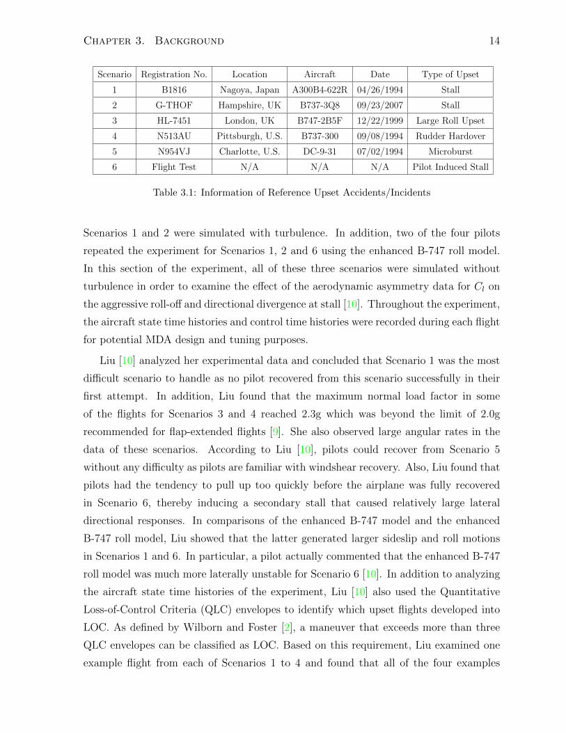
3.1.2 Upset Recovery Experiment
Liu [10] conducted a piloted upset recovery experiment in the UTIAS Flight Research
Simulator (FRS) to examine the aircraft behavior at upset using both the enhanced B-
747 model and the enhanced B-747 roll model. In this experiment, six upset scenarios
were designed based on past accidents and flight test data for piloted recoveries. These
scenarios are summarized in Table 3.1.
Four pilots participated in Liu’s experiment [10]. All of them flew the simulated
aircraft and recovered from the six pre-programmed upset conditions using the enhanced
B-747 model with the motion-base turned off. In this part of the experiment, only
Chapter 3. Background 14
Scenario Registration No. Location Aircraft Date Type of Upset
1 B1816 Nagoya, Japan A300B4-622R 04/26/1994 Stall
2 G-THOF Hampshire, UK B737-3Q8 09/23/2007 Stall
3 HL-7451 London, UK B747-2B5F 12/22/1999 Large Roll Upset
4 N513AU Pittsburgh, U.S. B737-300 09/08/1994 Rudder Hardover
5 N954VJ Charlotte, U.S. DC-9-31 07/02/1994 Microburst
6 Flight Test N/A N/A N/A Pilot Induced Stall
Table 3.1: Information of Reference Upset Accidents/Incidents
Scenarios 1 and 2 were simulated with turbulence. In addition, two of the four pilots
repeated the experiment for Scenarios 1, 2 and 6 using the enhanced B-747 roll model.
In this section of the experiment, all of these three scenarios were simulated without
turbulence in order to examine the effect of the aerodynamic asymmetry data for Cl on
the aggressive roll-off and directional divergence at stall [10]. Throughout the experiment,
the aircraft state time histories and control time histories were recorded during each flight
for potential MDA design and tuning purposes.
Liu [10] analyzed her experimental data and concluded that Scenario 1 was the most
difficult scenario to handle as no pilot recovered from this scenario successfully in their
first attempt. In addition, Liu found that the maximum normal load factor in some
of the flights for Scenarios 3 and 4 reached 2.3g which was beyond the limit of 2.0g
recommended for flap-extended flights [9]. She also observed large angular rates in the
data of these scenarios. According to Liu [10], pilots could recover from Scenario 5
without any difficulty as pilots are familiar with windshear recovery. Also, Liu found that
pilots had the tendency to pull up too quickly before the airplane was fully recovered
in Scenario 6, thereby inducing a secondary stall that caused relatively large lateral
directional responses. In comparisons of the enhanced B-747 model and the enhanced
B-747 roll model, Liu showed that the latter generated larger sideslip and roll motions
in Scenarios 1 and 6. In particular, a pilot actually commented that the enhanced B-747
roll model was much more laterally unstable for Scenario 6 [10]. In addition to analyzing
the aircraft state time histories of the experiment, Liu [10] also used the Quantitative
Loss-of-Control Criteria (QLC) envelopes to identify which upset flights developed into
LOC. As defined by Wilborn and Foster [2], a maneuver that exceeds more than three
QLC envelopes can be classified as LOC. Based on this requirement, Liu examined one
example flight from each of Scenarios 1 to 4 and found that all of the four examples
Chapter 3. Background 15
resulted in LOC as they all exceeded more than three of the five QLC envelopes [10].
3.2 Platform Motion Cues
3.2.1 Definition of Motion Cues and Motion Cueing Errors
When flying flight simulators, pilots receive information representative of the actual mo-
tion which they would expect in an aircraft. They use this representative information as
cues to interpret the flight conditions and make decisions regarding their control inputs.
The most common cues presented in simulators are visual cues generated by the image
generator system and instruments, gravito-inertial cues generated by the simulator mo-
tion platform, proprioceptive cues created by the simulator force feel system, and aural
cues generated by the sound system [26]. According to Grant [30], motion cues could be
interpreted as any cue humans use to identify their motion, or any motion humans use as
a cue. This report will only focus on the latter because it is what MDAs directly control
and produce. For simplicity, this report will refer a motion cue to be “a signal generated
by motion through inertial space which is sensed by the pilot and/or guides the pilot’s
behavior” as defined in Reference (P.114, [30]). Grant emphasized that “[t]he signal it-
self is not the cue, only the human’s use or sense of the signal defines a cue” (P.113,
[30]). “Any simulator movement is therefore considered as motion, but not necessarily
as motion cue” (P.2, [31]).
All simulator motion platforms have very limited travel as compared to real aircraft.
During simulation, the desired aircraft motions are scaled, limited and filtered using
MDAs to produce representative motions without hitting the physical limits of the sim-
ulator [32]; therefore, almost all motion cues provided by the simulator differ from what
is expected in the aircraft [26, 33]. Grant [30] categorized motion cue errors into four
distinct types. According to Grant [30], false cues include motion cues in the simulator
which are in the opposite direction to what are in the aircraft, motion cues in the simu-
lator which are not expected in the aircraft and sustained motion cues in the simulator
which are distorted at relatively high frequency as compared to those in the aircraft. In
contrast, missing cues refer to motion cues that are not provided in the simulator, but
are expected in the aircraft. They do not degrade the motion fidelity as much as false
cues do and generally do not lead to significant pilot complaints [30]. Phase errors are
generated by high-pass filters in MDAs in the form of phase lead at frequencies near
Chapter 3. Background 16
and below the filters’ break frequencies. They are the most noticeable near the break
frequencies of the high-pass filters and become less significant as frequency decreases due
to the signal attenuation performed by the high-pass filters. Lastly, scaling errors are
resulted when the aircraft inputs are scaled down by MDAs and extreme scaling of the
aircraft motion can actually lead to missing cues.
3.2.2 Benefits of Motion Cues for Upset Recovery Training
The usefulness of simulator platform motion for training has always been debated. Re-
searchers are still uncertain as to whether motion leads to an improvement in transfer of
training. However, research has shown that motion strongly affects pilot performance in
certain situations [33]. In fact, the situations for which motion affects performance will
often arise during the extreme flight conditions experienced during aircraft upset. For
instance, White and Cooper [20] examined the lateral-directional stability at wings-level
flight at a poststall angle of attack. Their results showed that roll motion allowed pilots
to have significantly better lateral-directional control over the airplane. In the study of
Bergeron et al. [21], it was shown that the addition of motion did not alter the mean
square error appreciably in one-axis compensatory control tasks, but led to both an in-
crease in system bandwidth and a reduction in mean square error in tasks involving two
axes (pitch and roll, or pitch and yaw). Meiry [22] investigated the motion effects on
the human control characteristics in stable and unstable systems during a single-axis roll
tracking task. Meiry showed that although motion cues alone did not allow complete
control of the simulator attitude, the combination of motion and visual cues resulted in
better performance than when solely visual cues were presented. This was especially true
with unstable systems because motion cues further enhanced the pilot’s ability to stabi-
lize the system near the limit of controllability [22]. Stapleford et al. [23] also performed
a single-axis roll control task with a disturbance input and showed that the contribution
of motion feedback was higher if the task required more pilot lead, which means the
system was more unstable. The same result has been confirmed by Shirley and Young
[24]. In summary, previous research found evidence of the positive effects of simulator
motion on pilot performance in maneuvers comparable to airplane upset. Therefore, it
is worthwhile to research improvements in simulator motion to generate useful motion
cues during UPRT.
Chapter 3. Background 17
3.3 UTIAS Classical Motion Drive Algorithm
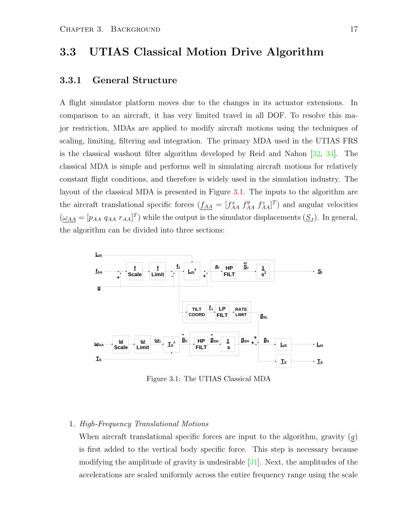
3.3.1 General Structure
A flight simulator platform moves due to the changes in its actuator extensions. In
comparison to an aircraft, it has very limited travel in all DOF. To resolve this ma-
jor restriction, MDAs are applied to modify aircraft motions using the techniques of
scaling, limiting, filtering and integration. The primary MDA used in the UTIAS FRS
is the classical washout filter algorithm developed by Reid and Nahon [32, 34]. The
classical MDA is simple and performs well in simulating aircraft motions for relatively
constant flight conditions, and therefore is widely used in the simulation industry. The
layout of the classical MDA is presented in Figure 3.1. The inputs to the algorithm are
the aircraft translational specific forces (fAA = [fxAA fyAA f
zAA]T ) and angular velocities
(ωAA = [pAA qAA rAA]T ) while the output is the simulator displacements (SI). In general,
the algorithm can be divided into three sections:
f
Scale
f
Limit
HP
FILT
1
s2LIS
x
RATE
LIMIT
LIS
fAA
f1 a I
.. S I
SI
f L
ω
Scale
ω
Limit
HP
FILT
1
s TS
xω1
.
βC βSH
+
++ LIS
TS
ωAA
TS
LIS
TS
βS
βSL
+ -
g
LP
FILTTILT
COORD
.
βSH
Figure 3.1: The UTIAS Classical MDA
1. High-Frequency Translational Motions
When aircraft translational specific forces are input to the algorithm, gravity (g)
is first added to the vertical body specific force. This step is necessary because
modifying the amplitude of gravity is undesirable [31]. Next, the amplitudes of the
accelerations are scaled uniformly across the entire frequency range using the scale
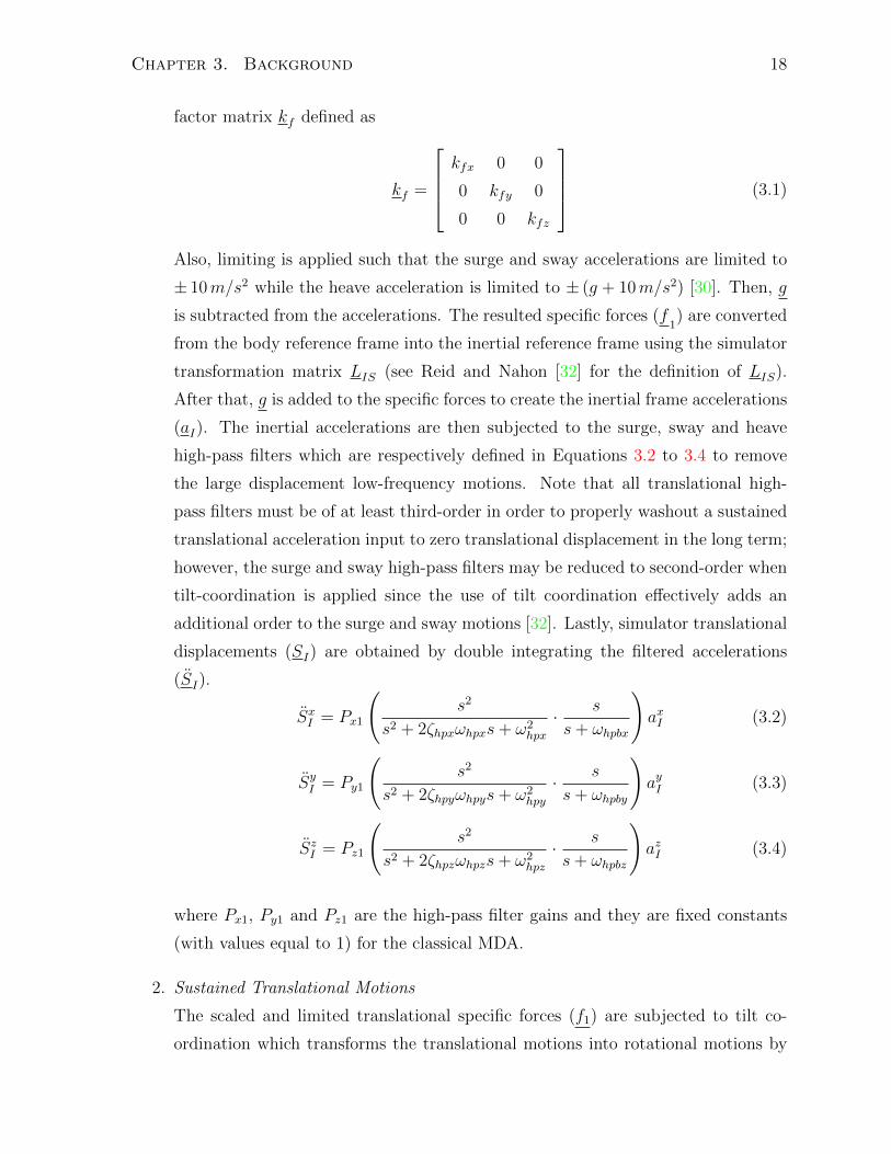
Chapter 3. Background 18
factor matrix kf defined as
kf =
kfx 0 0
0 kfy 0
0 0 kfz
(3.1)
Also, limiting is applied such that the surge and sway accelerations are limited to
± 10m/s2 while the heave acceleration is limited to ± (g + 10m/s2) [30]. Then, g
is subtracted from the accelerations. The resulted specific forces (f1) are converted
from the body reference frame into the inertial reference frame using the simulator
transformation matrix LIS (see Reid and Nahon [32] for the definition of LIS).
After that, g is added to the specific forces to create the inertial frame accelerations
(aI). The inertial accelerations are then subjected to the surge, sway and heave
high-pass filters which are respectively defined in Equations 3.2 to 3.4 to remove
the large displacement low-frequency motions. Note that all translational high-
pass filters must be of at least third-order in order to properly washout a sustained
translational acceleration input to zero translational displacement in the long term;
however, the surge and sway high-pass filters may be reduced to second-order when
tilt-coordination is applied since the use of tilt coordination effectively adds an
additional order to the surge and sway motions [32]. Lastly, simulator translational
displacements (SI) are obtained by double integrating the filtered accelerations
(SI).
SxI = Px1
(s2
s2 + 2ζhpxωhpxs+ ω2hpx
· s
s+ ωhpbx
)axI (3.2)
SyI = Py1
(s2
s2 + 2ζhpyωhpys+ ω2hpy
· s
s+ ωhpby
)ayI (3.3)
SzI = Pz1
(s2
s2 + 2ζhpzωhpzs+ ω2hpz
· s
s+ ωhpbz
)azI (3.4)
where Px1, Py1 and Pz1 are the high-pass filter gains and they are fixed constants
(with values equal to 1) for the classical MDA.
2. Sustained Translational Motions
The scaled and limited translational specific forces (f1) are subjected to tilt co-
ordination which transforms the translational motions into rotational motions by
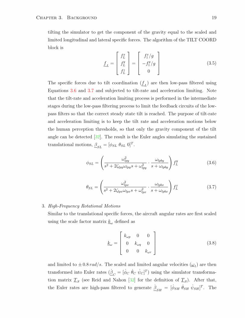
Chapter 3. Background 19
tilting the simulator to get the component of the gravity equal to the scaled and
limited longitudinal and lateral specific forces. The algorithm of the TILT COORD
block is
fL
=
fxL
f yL
f zL
=
fx1 /g
−f y1 /g0
(3.5)
The specific forces due to tilt coordination (fL) are then low-pass filtered using
Equations 3.6 and 3.7 and subjected to tilt-rate and acceleration limiting. Note
that the tilt-rate and acceleration limiting process is performed in the intermediate
stages during the low-pass filtering process to limit the feedback circuits of the low-
pass filters so that the correct steady state tilt is reached. The purpose of tilt-rate
and acceleration limiting is to keep the tilt rate and acceleration motions below
the human perception thresholds, so that only the gravity component of the tilt
angle can be detected [32]. The result is the Euler angles simulating the sustained
translational motions, βSL
= [φSL θSL 0]T .
φSL =
(ω2lpy
s2 + 2ζlpyωlpys+ ω2lpy
· ωlpbys+ ωlpby
)f yL (3.6)
θSL =
(ω2lpx
s2 + 2ζlpxωlpxs+ ω2lpx
· ωlpbxs+ ωlpbx
)fxL (3.7)
3. High-Frequency Rotational Motions
Similar to the translational specific forces, the aircraft angular rates are first scaled
using the scale factor matrix kω defined as
kω =
kωp 0 0
0 kωq 0
0 0 kωr
(3.8)
and limited to ± 0.8 rad/s. The scaled and limited angular velocities (ω1) are then
transformed into Euler rates (βC
= [φC θC ψC ]T ) using the simulator transforma-
tion matrix T S (see Reid and Nahon [32] for the definition of T S). After that,
the Euler rates are high-pass filtered to generate βSH
= [φSH θSH ψSH ]T . The
Chapter 3. Background 20
high-pass angular filters are defined as
φSH =
Py4
(s2
s2 + 2ζhpφωhpφs+ ω2hpφ
)φC if Oφ = 2
Py4
(s
s+ ωhpφ
)φC if Oφ = 1
(3.9)
θSH =
Px4
(s2
s2 + 2ζhpθωhpθs+ ω2hpθ
)θC if Oθ = 2
Px4
(s
s+ ωhpθ
)θC if Oθ = 1
(3.10)
ψSH =
Pψ1
(s2
s2 + 2ζhpψωhpψs+ ω2hpψ
)ψC if Oψ = 2
Pψ1
(s
s+ ωhpψ
)ψC if Oψ = 1
(3.11)
where Px4, Py4 and Pψ1 are the high-pass filter gains which are fixed constants
(equal to 1) for the classical MDA, and Oφ, Oθ and Oψ define the orders of the
angular high-pass filters. Note that the rotational high-pass filters may be indepen-
dently reduced to first-order, but the filters have to be second-order to ensure that
sustained angular rates are properly washed out to zero angular displacements in
the long term [32]. By integrating the outputs from Equations 3.9 to 3.11, the Eu-
ler angles (βSH
) can be obtained. Using βSH
and βSL
resulting from the sustained
specific forces, the total simulator Euler angles (βS) can be calculated by
βS
= βSH
+ (βSL
)LIM (3.12)
where LIM represents the internal tilt-rate and acceleration limiting process.
3.4 UTIAS Adaptive Motion Drive Algorithm
3.4.1 General Structure
The UTIAS Adaptive Motion Drive Algorithm was originally developed by Reid and
Nahon [32, 34]. It was found to be slightly preferred over the classical MDA when tested
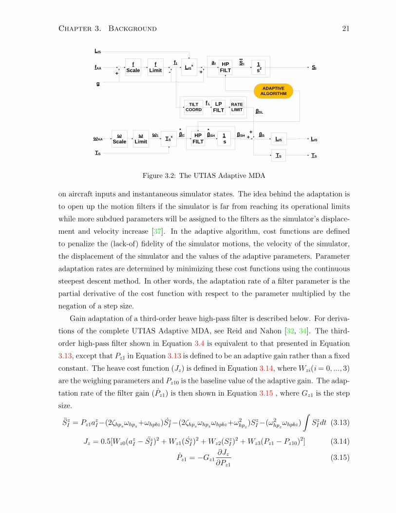
in piloted experiments [35, 36]. As shown in Figure 3.2, the adaptive MDA is a modifi-
cation of the classical MDA with high-pass filter parameters adapted in real-time based
Chapter 3. Background 21
f
Scale
f
Limit
HP
FILT
1
s2LIS
x
RATE
LIMIT
LIS
fAA
f1 a I
.. S I
SI
f L
ω
Scale
ω
Limit
HP
FILT
1
s TS
xω1
.
βC βSH
+
++ LIS
TS
ωAA
TS
LIS
TS
βS
βSL
+ -
gADAPTIVE
ALGORITHM
LP
FILTTILT
COORD
.
βSH
Figure 3.2: The UTIAS Adaptive MDA
on aircraft inputs and instantaneous simulator states. The idea behind the adaptation is
to open up the motion filters if the simulator is far from reaching its operational limits
while more subdued parameters will be assigned to the filters as the simulator’s displace-
ment and velocity increase [37]. In the adaptive algorithm, cost functions are defined
to penalize the (lack-of) fidelity of the simulator motions, the velocity of the simulator,
the displacement of the simulator and the values of the adaptive parameters. Parameter
adaptation rates are determined by minimizing these cost functions using the continuous
steepest descent method. In other words, the adaptation rate of a filter parameter is the
partial derivative of the cost function with respect to the parameter multiplied by the
negation of a step size.
Gain adaptation of a third-order heave high-pass filter is described below. For deriva-
tions of the complete UTIAS Adaptive MDA, see Reid and Nahon [32, 34]. The third-
order high-pass filter shown in Equation 3.4 is equivalent to that presented in Equation
3.13, except that Pz1 in Equation 3.13 is defined to be an adaptive gain rather than a fixed
constant. The heave cost function (Jz) is defined in Equation 3.14, where Wzi(i = 0, ..., 3)
are the weighing parameters and Pz10 is the baseline value of the adaptive gain. The adap-
tation rate of the filter gain (Pz1) is then shown in Equation 3.15 , where Gz1 is the step
size.
SzI = Pz1azI−(2ζhpzωhpz+ωhpbz)SzI−(2ζhpzωhpzωhpbz+ω
2hpz
)SzI−(ω2hpzωhpbz)
∫SzIdt (3.13)
Jz = 0.5[Wz0(azI − SzI )2 +Wz1(SzI )2 +Wz2(SzI )2 +Wz3(Pz1 − Pz10)2] (3.14)
Pz1 = −Gz1∂Jz∂Pz1
(3.15)
Chapter 3. Background 22
3.4.2 Problems with the Original UTIAS Adaptive MDA
In the original adaptive algorithm, the parameter adaptation rates are evaluated using an
analytical approach. O’Toole [37] investigated the performance of this analytical adap-
tive algorithm using the third-order gain adaptive heave filter and found two problems
in the algorithm. First, the simulated response of the original adaptive MDA to a heave
acceleration step input contained undesired oscillations [37]. O’Toole demonstrated that
errors in the integration process caused high frequency oscillations in the acceleration
response and this problem could be solved by using a higher integration rate or a high
order integration scheme. On the other hand, the transient response of the cost function
fidelity term resulted in large amplitude low frequency oscillations in the simulated heave
acceleration [37]. O’Toole suggests that the transient oscillations could be removed by
setting Wz0 to zero, but doing so would destroy the adaptation purpose of the algorithm.
Second, the gain adaptation of the third-order filter ceased regardless of the large differ-
ence between the aircraft acceleration and the simulator translational acceleration [37].
O’Toole studied the contribution of the cost function fidelity term to the gain adaptation
rate using a simplified cost function defined as
Jz = (azI − SzI )2 (3.16)
Ideally, large errors in the fidelity term should contribute to a positive gain adaptation
rate and force the filter gain to keep increasing in order to minimize the cost function. In
fact, without any other penalty and a large step size the gain should increase such that the
simulator acceleration almost matches the aircraft acceleration. O’Toole [37], however,
observed that the fidelity term barely affected the adaptation rate since it reached a
steady state of zero. In other words,
∂Jz∂Pz1
= −2(azI − SzI )∂SzI∂Pz1
→ 0 (3.17)
According to Equation 3.13, ∂SzI /∂Pz1 in Equation 3.17 can be expressed as
∂SzI∂Pz1
= azI −∂a
∂Pz1(3.18)
where a = (2ζhpzωhpz + ωhpbz)SzI + (2ζhpzωhpzωhpbz + ω2hpz
)SzI + (ω2hpzωhpbz)
∫SzIdt. As
defined by Reid and Nahon [32], it is assumed in the analytical algorithm of the original
adaptive MDA that
∂
∂Pz1
(d2SzIdt2
)=
d2
dt2
(∂SzI∂Pz1
)=
d
dt
(∂SzI∂Pz1
)(3.19)
Chapter 3. Background 23
O’Toole [37] argued that ∂a/∂Pz1 calculated based on the above assumption equaled azI
at steady state. As a result, ∂SzI /∂Pz1 and Equation 3.17 would reach a steady state of
zero and the gain adaptation would terminate regardless of any difference between the
aircraft input and simulator output.
In response to the problems of the original adaptive MDA, O’Toole [37] suggests
evaluating the gain adaptation rate numerically. In the numerical adaptive algorithm,
∂Jz/∂Pz1 which governs Pz1 is defined as
∂Jz∂Pz1
= lim4Pz1→0
[Jz(a
zI , S
zI , S
zI , S
zI , Pz1 +4Pz1)− Jz(azI , SzI , SzI , SzI , Pz1)
4Pz1
](3.20)
where the motion variables (SzI , SzI and SzI ) on the left cost function must be evaluated
using the perturbed gain (Pz1 +4Pz1) while those on the right cost function must be
determined based on Pz1 [37]. O’Toole then simulated the heave acceleration step input
again using the numerical approach. He showed that the numerical estimates of the
adaptation rates differed significantly from the analytical estimates while the numerical
estimates did not contain undesired oscillations or improper termination of the parameter
adaptation.
Chapter 4
Motion Fidelity Criteria for
Coordinated Roll Upsets
The ability to simulate a coordinated roll maneuver greatly affects the motion fidelity
of a simulator [38]. When an aircraft rolls and turns, the specific forces resulting from
the projection of gravity in the body-axis lateral direction is canceled by the centripetal
force. When a simulator rolls, however, no turning is performed and consequently, the
gravity component in the lateral body axis remains uncanceled and becomes a false
motion cue. One way to compensate these false lateral motion cues is to generate lateral
inertial acceleration as the simulator rolls. Unfortunately, this is not sufficient for upset
simulation because the simulator is unlikely to have enough travel to generate the required
lateral acceleration [25]. The other method for reducing the false cue is to high-pass filter
the aircraft roll motion so the onset cues are presented but the simulator rolls back to
zero roll-angle in the steady-state.
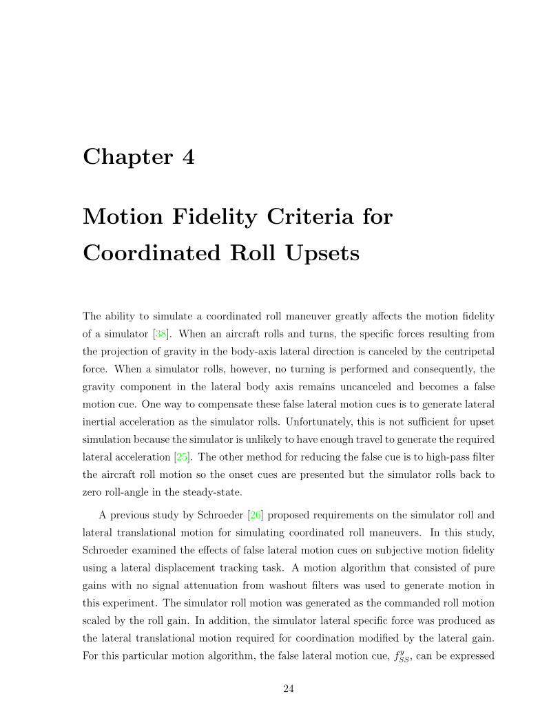
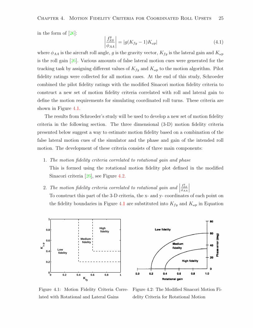
A previous study by Schroeder [26] proposed requirements on the simulator roll and
lateral translational motion for simulating coordinated roll maneuvers. In this study,
Schroeder examined the effects of false lateral motion cues on subjective motion fidelity
using a lateral displacement tracking task. A motion algorithm that consisted of pure
gains with no signal attenuation from washout filters was used to generate motion in
this experiment. The simulator roll motion was generated as the commanded roll motion
scaled by the roll gain. In addition, the simulator lateral specific force was produced as
the lateral translational motion required for coordination modified by the lateral gain.
For this particular motion algorithm, the false lateral motion cue, f ySS, can be expressed
24
Chapter 4. Motion Fidelity Criteria for Coordinated Roll Upsets 25
in the form of [26]: ∣∣∣∣ f ySSφAA
∣∣∣∣ = |g(Kfy − 1)Kωp| (4.1)
where φAA is the aircraft roll angle, g is the gravity vector, Kfy is the lateral gain and Kωp
is the roll gain [26]. Various amounts of false lateral motion cues were generated for the
tracking task by assigning different values of Kfy and Kωp to the motion algorithm. Pilot
fidelity ratings were collected for all motion cases. At the end of this study, Schroeder
combined the pilot fidelity ratings with the modified Sinacori motion fidelity criteria to
construct a new set of motion fidelity criteria correlated with roll and lateral gain to
define the motion requirements for simulating coordinated roll turns. These criteria are
shown in Figure 4.1.
The results from Schroeder’s study will be used to develop a new set of motion fidelity
criteria in the following section. The three dimensional (3-D) motion fidelity criteria
presented below suggest a way to estimate motion fidelity based on a combination of the
false lateral motion cues of the simulator and the phase and gain of the intended roll
motion. The development of these criteria consists of three main components:
1. The motion fidelity criteria correlated to rotational gain and phase
This is formed using the rotational motion fidelity plot defined in the modified
Sinacori criteria [26], see Figure 4.2.
2. The motion fidelity criteria correlated to rotational gain and∣∣∣ fySSφAA
∣∣∣To construct this part of the 3-D criteria, the x- and y- coordinates of each point on
the fidelity boundaries in Figure 4.1 are substituted into Kfy and Kωp in Equation
0 0.2 0.4 0.6 0.8 10
0.2
0.4
0.6
0.8
1
Kfy
Kω
p
High fidelity
Medium fidelity
Low fidelity
Figure 4.1: Motion Fidelity Criteria Corre-
lated with Rotational and Lateral Gains
Figure 4.2: The Modified Sinacori Motion Fi-
delity Criteria for Rotational Motion
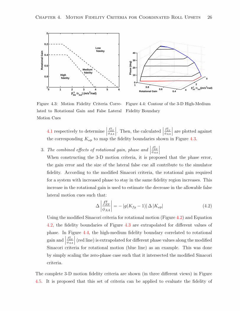
Chapter 4. Motion Fidelity Criteria for Coordinated Roll Upsets 26
0 1 2 3 4 5 6
0
0.2
0.4
0.6
0.8
1
|fSS y /φ
AA| (m/s2/rad)
Ro
tati
on
al G
ain
High fidelity
Medium fidelity
Low fidelity
Figure 4.3: Motion Fidelity Criteria Corre-
lated to Rotational Gain and False Lateral
Motion Cues
0
2
40.40.6
0.810
10
20
30
40
|fSS y /φ
AA|(m/s2/rad)
Rotational Gain
Ph
ase
(deg
)
Figure 4.4: Contour of the 3-D High-Medium
Fidelity Boundary
4.1 respectively to determine∣∣∣ fySSφAA
∣∣∣. Then, the calculated∣∣∣ fySSφAA
∣∣∣ are plotted against
the corresponding Kωp to map the fidelity boundaries shown in Figure 4.3.
3. The combined effects of rotational gain, phase and∣∣∣ fySSφAA
∣∣∣When constructing the 3-D motion criteria, it is proposed that the phase error,
the gain error and the size of the lateral false cue all contribute to the simulator
fidelity. According to the modified Sinacori criteria, the rotational gain required
for a system with increased phase to stay in the same fidelity region increases. This
increase in the rotational gain is used to estimate the decrease in the allowable false
lateral motion cues such that:
∆
∣∣∣∣ f ySSφAA
∣∣∣∣ = − |g(Kfy − 1)|∆ |Kωp| (4.2)
Using the modified Sinacori criteria for rotational motion (Figure 4.2) and Equation
4.2, the fidelity boundaries of Figure 4.3 are extrapolated for different values of
phase. In Figure 4.4, the high-medium fidelity boundary correlated to rotational
gain and∣∣∣ fySSφAA
∣∣∣ (red line) is extrapolated for different phase values along the modified
Sinacori criteria for rotational motion (blue line) as an example. This was done
by simply scaling the zero-phase case such that it intersected the modified Sinacori
criteria.
The complete 3-D motion fidelity criteria are shown (in three different views) in Figure
4.5. It is proposed that this set of criteria can be applied to evaluate the fidelity of
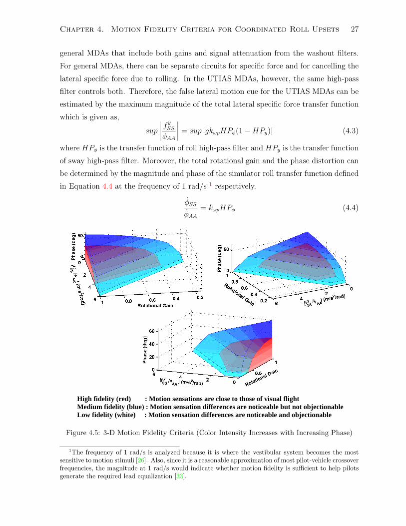
Chapter 4. Motion Fidelity Criteria for Coordinated Roll Upsets 27
general MDAs that include both gains and signal attenuation from the washout filters.
For general MDAs, there can be separate circuits for specific force and for cancelling the
lateral specific force due to rolling. In the UTIAS MDAs, however, the same high-pass
filter controls both. Therefore, the false lateral motion cue for the UTIAS MDAs can be
estimated by the maximum magnitude of the total lateral specific force transfer function
which is given as,
sup
∣∣∣∣ f ySSφAA
∣∣∣∣ = sup |gkωpHPφ(1−HPy)| (4.3)
where HPφ is the transfer function of roll high-pass filter and HPy is the transfer function
of sway high-pass filter. Moreover, the total rotational gain and the phase distortion can
be determined by the magnitude and phase of the simulator roll transfer function defined
in Equation 4.4 at the frequency of 1 rad/s 1 respectively.
φSS
φAA= kωpHPφ (4.4)
High fidelity (red) : Motion sensations are close to those of visual flightMedium fidelity (blue) : Motion sensation differences are noticeable but not objectionableLow fidelity (white) : Motion sensation differences are noticeable and objectionable
Figure 4.5: 3-D Motion Fidelity Criteria (Color Intensity Increases with Increasing Phase)
1The frequency of 1 rad/s is analyzed because it is where the vestibular system becomes the mostsensitive to motion stimuli [26]. Also, since it is a reasonable approximation of most pilot-vehicle crossoverfrequencies, the magnitude at 1 rad/s would indicate whether motion fidelity is sufficient to help pilotsgenerate the required lead equalization [33].
Chapter 5
Body Frame Filtering
Typical MDAs, including the UTIAS Classical MDA, are designed to perform high-pass
filtering in the inertial reference frame. The advantage of inertial high-pass filters is that
they ensure the simulator does not drift off into stops in the long term [32], but the
combination of the inertial high-pass filtering and the reference frame rotation between
the body and inertial reference frames can lead to significant cross-coupling among the
simulator body-axis specific force components [32]. For maneuvers with moderate aircraft
motions, the effects of cross-coupling can be assumed to be negligible; however, cross-
coupling could become significant when simulating upset conditions where the aircraft
and simulator attitudes can be large. According to Reid and Nahon [32], cross-coupling
can be avoided if body frame filters are used instead of inertial frame filters, with the
trade-off being drifting of the simulator position in the long term. This argument leads
to the idea of combining body frame filters with inertial frame filters in order to reduce
cross-coupling while ensuring motion commands remain within the motion system limits.
This chapter focuses on the experiment performed to investigate whether the com-
bination of body and inertial filters can reduce motion cue errors during upset recovery
simulation. In this experiment, the simulated aircraft state time histories of the six upset
scenarios collected by Liu as discussed in Section 3.1.2 were used as the aircraft inputs
to the MDAs. They were first simulated using the original classical MDA that involved
only inertial filters (see Section 3.3). The inertial filter parameters of the classical MDA
were tuned for each scenario to match the simulator specific forces with the correspond-
ing aircraft inputs and to minimize both the norm of the perception vector and the root
28
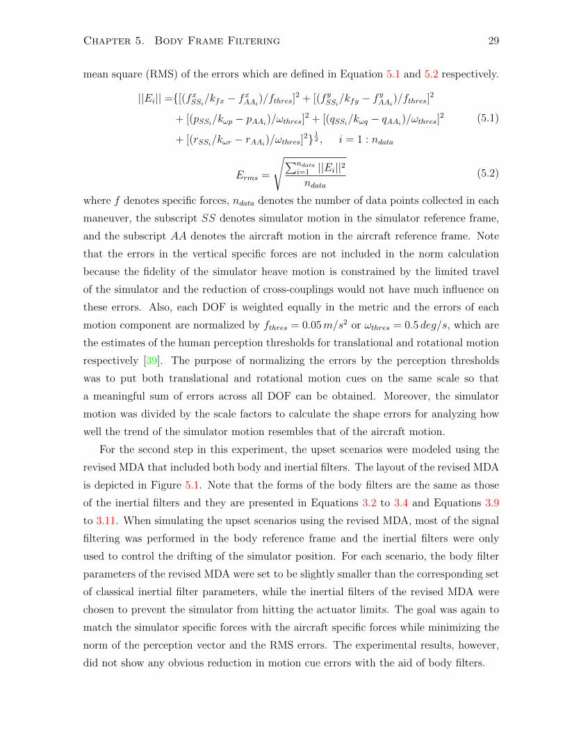
Chapter 5. Body Frame Filtering 29
mean square (RMS) of the errors which are defined in Equation 5.1 and 5.2 respectively.
||Ei|| =[(fxSSi/kfx − fxAAi
)/fthres]2 + [(f ySSi/kfy − f
yAAi
)/fthres]2
+ [(pSSi/kωp − pAAi)/ωthres]2 + [(qSSi/kωq − qAAi)/ωthres]2
+ [(rSSi/kωr − rAAi)/ωthres]212 , i = 1 : ndata
(5.1)
Erms =
√∑ndatai=1 ||Ei||2ndata
(5.2)
where f denotes specific forces, ndata denotes the number of data points collected in each
maneuver, the subscript SS denotes simulator motion in the simulator reference frame,
and the subscript AA denotes the aircraft motion in the aircraft reference frame. Note
that the errors in the vertical specific forces are not included in the norm calculation
because the fidelity of the simulator heave motion is constrained by the limited travel
of the simulator and the reduction of cross-couplings would not have much influence on
these errors. Also, each DOF is weighted equally in the metric and the errors of each
motion component are normalized by fthres = 0.05m/s2 or ωthres = 0.5 deg/s, which are
the estimates of the human perception thresholds for translational and rotational motion
respectively [39]. The purpose of normalizing the errors by the perception thresholds
was to put both translational and rotational motion cues on the same scale so that
a meaningful sum of errors across all DOF can be obtained. Moreover, the simulator
motion was divided by the scale factors to calculate the shape errors for analyzing how
well the trend of the simulator motion resembles that of the aircraft motion.
For the second step in this experiment, the upset scenarios were modeled using the
revised MDA that included both body and inertial filters. The layout of the revised MDA
is depicted in Figure 5.1. Note that the forms of the body filters are the same as those
of the inertial filters and they are presented in Equations 3.2 to 3.4 and Equations 3.9
to 3.11. When simulating the upset scenarios using the revised MDA, most of the signal
filtering was performed in the body reference frame and the inertial filters were only
used to control the drifting of the simulator position. For each scenario, the body filter
parameters of the revised MDA were set to be slightly smaller than the corresponding set
of classical inertial filter parameters, while the inertial filters of the revised MDA were
chosen to prevent the simulator from hitting the actuator limits. The goal was again to
match the simulator specific forces with the aircraft specific forces while minimizing the
norm of the perception vector and the RMS errors. The experimental results, however,
did not show any obvious reduction in motion cue errors with the aid of body filters.
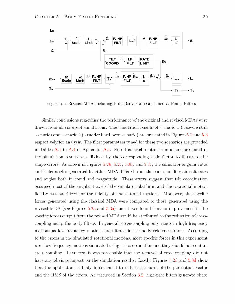
Chapter 5. Body Frame Filtering 30
f
Scale
f
Limit
FI HP
FILT
1
s2LIS
x
RATE
LIMIT
LIS
fAA
f1SI
f L
ω
Scale
ω
Limit
FI HP
FILT
1
s TS
xω1
.
βCβSH +
+ LIS
TS
ωAA
TS
LIS
TS
βS
βSL
+
+
-+
g
FB HP
FILT
gs
+
FB HP
FILT
LP
FILT
TILT
COORD
.
βSH
a I
.. S I
Figure 5.1: Revised MDA Including Both Body Frame and Inertial Frame Filters
Similar conclusions regarding the performance of the original and revised MDAs were
drawn from all six upset simulations. The simulation results of scenario 1 (a severe stall
scenario) and scenario 4 (a rudder hard-over scenario) are presented in Figures 5.2 and 5.3
respectively for analysis. The filter parameters tuned for these two scenarios are provided
in Tables A.1 to A.4 in Appendix A.1. Note that each motion component presented in
the simulation results was divided by the corresponding scale factor to illustrate the
shape errors. As shown in Figures 5.2b, 5.2c, 5.3b, and 5.3c, the simulator angular rates
and Euler angles generated by either MDA differed from the corresponding aircraft rates
and angles both in trend and magnitude. These errors suggest that tilt coordination
occupied most of the angular travel of the simulator platform, and the rotational motion
fidelity was sacrificed for the fidelity of translational motions. Moreover, the specific
forces generated using the classical MDA were compared to those generated using the
revised MDA (see Figures 5.2a and 5.3a) and it was found that no improvement in the
specific forces output from the revised MDA could be attributed to the reduction of cross-
coupling using the body filters. In general, cross-coupling only exists in high frequency
motions as low frequency motions are filtered in the body reference frame. According
to the errors in the simulated rotational motions, most specific forces in this experiment
were low frequency motions simulated using tilt-coordination and they should not contain
cross-coupling. Therefore, it was reasonable that the removal of cross-coupling did not
have any obvious impact on the simulation results. Lastly, Figures 5.2d and 5.3d show
that the application of body filters failed to reduce the norm of the perception vector
and the RMS of the errors. As discussed in Section 3.2, high-pass filters generate phase

Chapter 5. Body Frame Filtering 31
lead and signal attenuation; therefore, adding body filters to the original classical MDA
could generate additional phase errors and magnitude errors to the system. As suggested
by the norm of the perception vector and the RMS values, the phase lead and signal
attenuation generated by the body filters might have produced more or less the same
amount of errors as those removed by the reduction of cross-coupling.
In summary, the simulation results showed that the addition of body filters in the
classical MDA did not help to improve motion fidelity in upset recovery simulation.
It, however, might be worthwhile to investigate whether the reduction of cross-coupling
would have a greater impact on simulating maneuvers that require little tilt coordination.
Also, since there is no guideline regarding the tuning of the filter parameters, it may be
possible to tune the body filter parameters in a different way to minimize all phase errors,
magnitude errors and cross-coupling; therefore, the usefulness of body filters should be
further analyzed before the method of body frame filtering is dismissed.
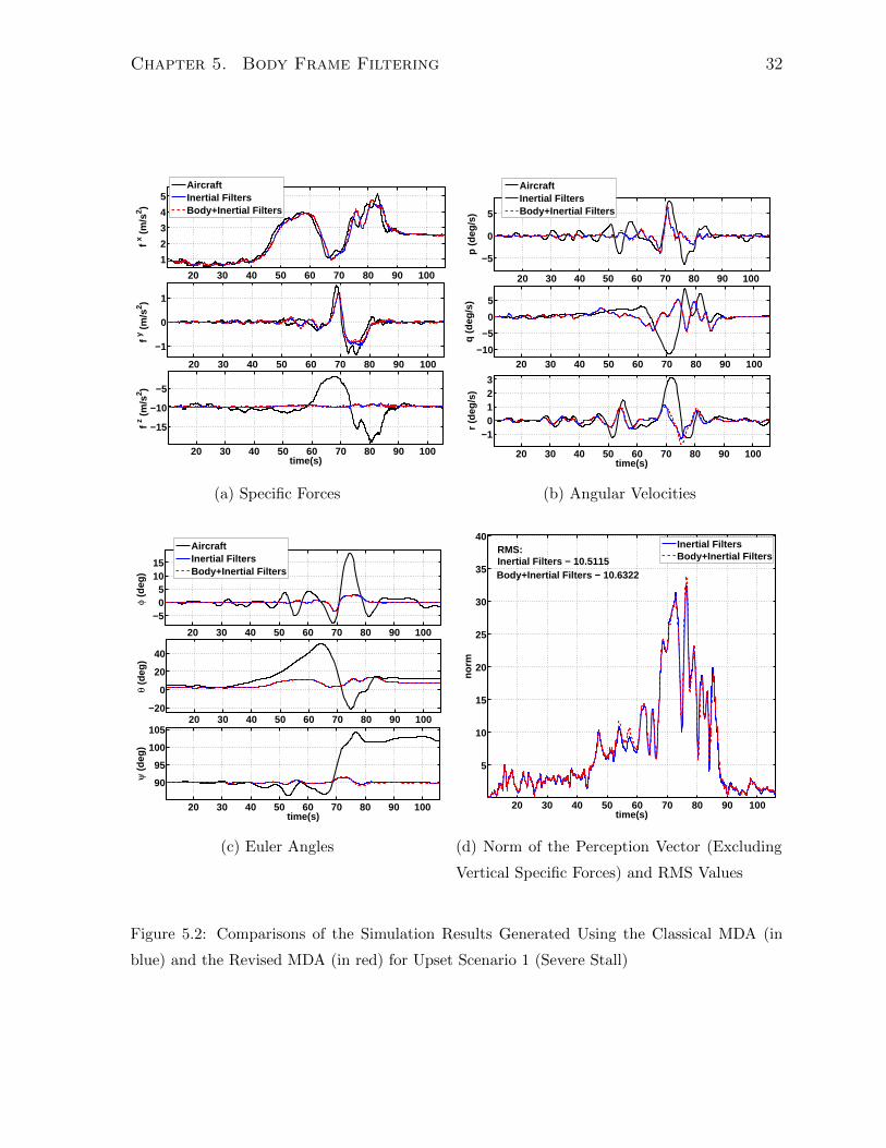
Chapter 5. Body Frame Filtering 32
20 30 40 50 60 70 80 90 100
1
2
3
4
5
f x (
m/s
2 )
20 30 40 50 60 70 80 90 100
−1
0
1
f y (
m/s
2 )
20 30 40 50 60 70 80 90 100
−15
−10
−5
time(s)
f z (
m/s
2 )
AircraftInertial FiltersBody+Inertial Filters
(a) Specific Forces
20 30 40 50 60 70 80 90 100
−5
0
5
p (
deg
/s)
20 30 40 50 60 70 80 90 100−10
−5
0
5
q (
deg
/s)
20 30 40 50 60 70 80 90 100
−10123
time(s)r
(deg
/s)
AircraftInertial FiltersBody+Inertial Filters
(b) Angular Velocities
20 30 40 50 60 70 80 90 100
−505
1015
φ (d
eg)
20 30 40 50 60 70 80 90 100−20
0
20
40
θ (d
eg)
20 30 40 50 60 70 80 90 100
90
95
100
105
time(s)
ψ (
deg
)
AircraftInertial FiltersBody+Inertial Filters
(c) Euler Angles
20 30 40 50 60 70 80 90 100
5
10
15
20
25
30
35
40
time(s)
no
rm
RMS: Inertial Filters − 10.5115Body+Inertial Filters − 10.6322
Inertial FiltersBody+Inertial Filters
(d) Norm of the Perception Vector (Excluding
Vertical Specific Forces) and RMS Values
Figure 5.2: Comparisons of the Simulation Results Generated Using the Classical MDA (in
blue) and the Revised MDA (in red) for Upset Scenario 1 (Severe Stall)
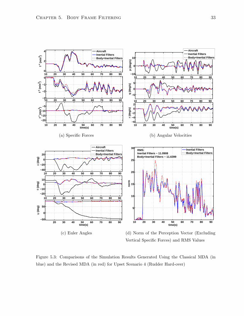
Chapter 5. Body Frame Filtering 33
10 20 30 40 50 60 70 80 900
2
4
f x (
m/s
2 )
10 20 30 40 50 60 70 80 90−3
−2
−1
0
f y (
m/s
2 )
10 20 30 40 50 60 70 80 90
−20
−15
−10
−5
time(s)
f z (
m/s
2 )
AircraftInertial FiltersBody+Inertial Filters
(a) Specific Forces
10 20 30 40 50 60 70 80 90−10
0
10
p (
deg
/s)
10 20 30 40 50 60 70 80 90
−5
0
5
q (
deg
/s)
10 20 30 40 50 60 70 80 90−6
−4
−2
0
2
time(s)r
(deg
/s)
AircraftInertial FiltersBody+Inertial Filters
(b) Angular Velocities
10 20 30 40 50 60 70 80 90−40
−20
0
20
φ (d
eg)
10 20 30 40 50 60 70 80 90
−20
−10
0
10
θ (d
eg)
20 30 40 50 60 70 80 90−50
0
50
time(s)
ψ (
deg
)
AircraftInertial FiltersBody+Inertial Filters
(c) Euler Angles
10 20 30 40 50 60 70 80 90
5
10
15
20
25
30
time(s)
no
rm
RMS: Inertial Filters − 11.0908Body+Inertial Filters − 11.6399
Inertial FiltersBody+Inertial Filters
(d) Norm of the Perception Vector (Excluding
Vertical Specific Forces) and RMS Values
Figure 5.3: Comparisons of the Simulation Results Generated Using the Classical MDA (in
blue) and the Revised MDA (in red) for Upset Scenario 4 (Rudder Hard-over)
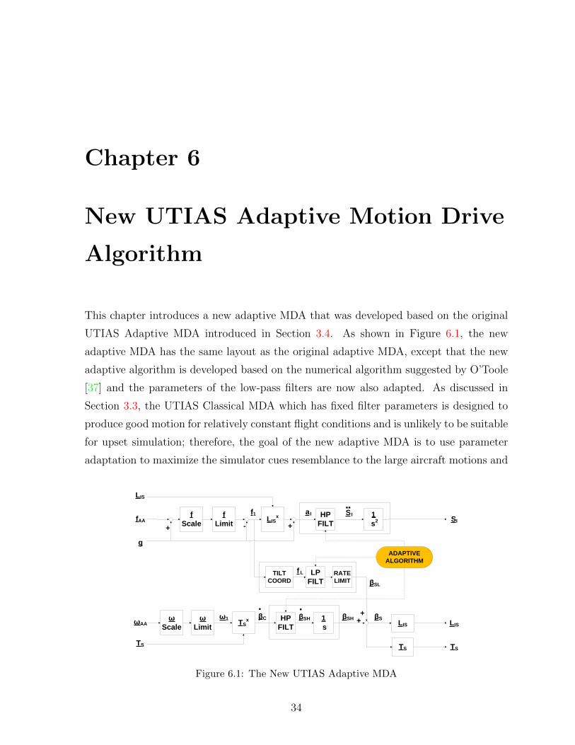
Chapter 6
New UTIAS Adaptive Motion Drive
Algorithm
This chapter introduces a new adaptive MDA that was developed based on the original
UTIAS Adaptive MDA introduced in Section 3.4. As shown in Figure 6.1, the new
adaptive MDA has the same layout as the original adaptive MDA, except that the new
adaptive algorithm is developed based on the numerical algorithm suggested by O’Toole
[37] and the parameters of the low-pass filters are now also adapted. As discussed in
Section 3.3, the UTIAS Classical MDA which has fixed filter parameters is designed to
produce good motion for relatively constant flight conditions and is unlikely to be suitable
for upset simulation; therefore, the goal of the new adaptive MDA is to use parameter
adaptation to maximize the simulator cues resemblance to the large aircraft motions and
f
Scale
f
Limit
HP
FILT
1
s2LIS
x
RATE
LIMIT
LIS
fAA
f1 a I
.. S I
SI
f L
ω
Scale
ω
Limit
HP
FILT
1
s TS
xω1
.
βC βSH
+
++ LIS
TS
ωAA
TS
LIS
TS
βS
βSL
+ -
g
ADAPTIVE
ALGORITHM
LP
FILTTILT
COORD
.
βSH
Figure 6.1: The New UTIAS Adaptive MDA
34
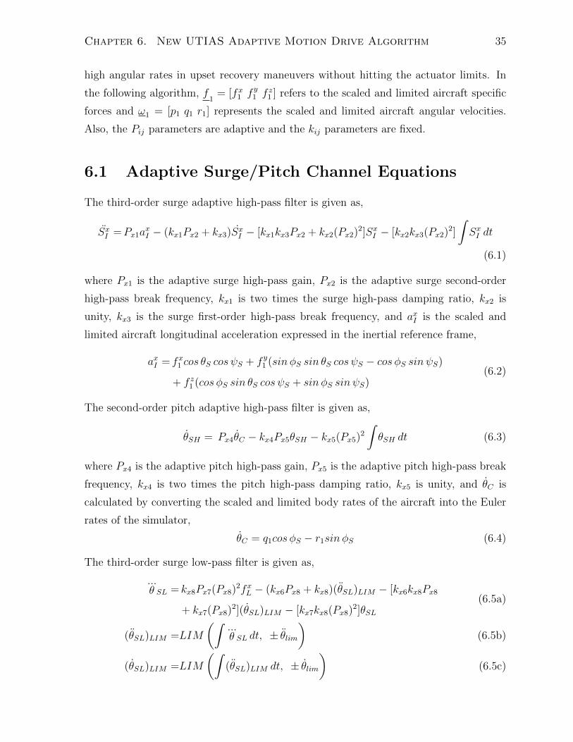
Chapter 6. New UTIAS Adaptive Motion Drive Algorithm 35
high angular rates in upset recovery maneuvers without hitting the actuator limits. In
the following algorithm, f1
= [fx1 f y1 f z1 ] refers to the scaled and limited aircraft specific
forces and ω1 = [p1 q1 r1] represents the scaled and limited aircraft angular velocities.
Also, the Pij parameters are adaptive and the kij parameters are fixed.
6.1 Adaptive Surge/Pitch Channel Equations
The third-order surge adaptive high-pass filter is given as,
SxI =Px1axI − (kx1Px2 + kx3)SxI − [kx1kx3Px2 + kx2(Px2)2]SxI − [kx2kx3(Px2)2]
∫SxI dt
(6.1)
where Px1 is the adaptive surge high-pass gain, Px2 is the adaptive surge second-order
high-pass break frequency, kx1 is two times the surge high-pass damping ratio, kx2 is
unity, kx3 is the surge first-order high-pass break frequency, and axI is the scaled and
limited aircraft longitudinal acceleration expressed in the inertial reference frame,
axI = fx1 cos θS cos ψS + f y1 (sin φS sin θS cos ψS − cos φS sinψS)
+ f z1 (cos φS sin θS cos ψS + sin φS sinψS)(6.2)
The second-order pitch adaptive high-pass filter is given as,
θSH = Px4θC − kx4Px5θSH − kx5(Px5)2
∫θSH dt (6.3)
where Px4 is the adaptive pitch high-pass gain, Px5 is the adaptive pitch high-pass break
frequency, kx4 is two times the pitch high-pass damping ratio, kx5 is unity, and θC is
calculated by converting the scaled and limited body rates of the aircraft into the Euler
rates of the simulator,
θC = q1cos φS − r1sin φS (6.4)
The third-order surge low-pass filter is given as,
...θ SL = kx8Px7(Px8)2fxL − (kx6Px8 + kx8)(θSL)LIM − [kx6kx8Px8
+ kx7(Px8)2](θSL)LIM − [kx7kx8(Px8)2]θSL(6.5a)
(θSL)LIM =LIM
(∫...θ SL dt, ± θlim
)(6.5b)
(θSL)LIM =LIM
(∫(θSL)LIM dt, ± θlim
)(6.5c)
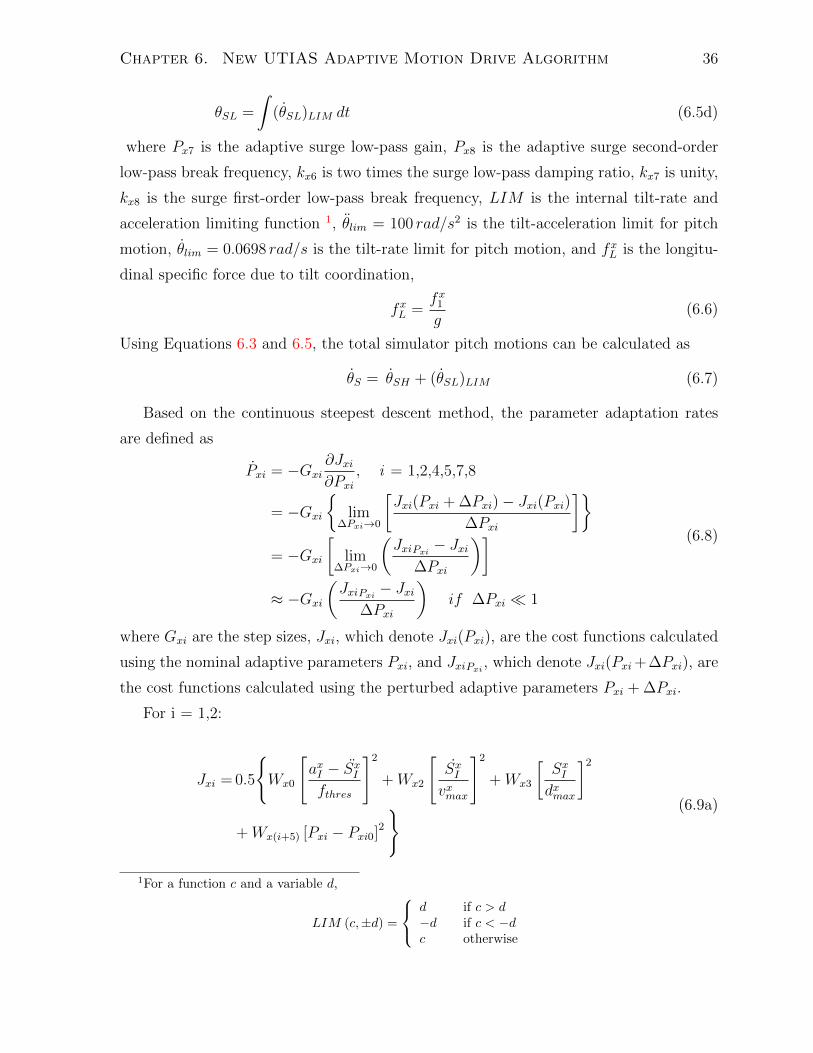
Chapter 6. New UTIAS Adaptive Motion Drive Algorithm 36
θSL =
∫(θSL)LIM dt (6.5d)
where Px7 is the adaptive surge low-pass gain, Px8 is the adaptive surge second-order
low-pass break frequency, kx6 is two times the surge low-pass damping ratio, kx7 is unity,
kx8 is the surge first-order low-pass break frequency, LIM is the internal tilt-rate and
acceleration limiting function 1, θlim = 100 rad/s2 is the tilt-acceleration limit for pitch
motion, θlim = 0.0698 rad/s is the tilt-rate limit for pitch motion, and fxL is the longitu-
dinal specific force due to tilt coordination,
fxL =fx1g
(6.6)
Using Equations 6.3 and 6.5, the total simulator pitch motions can be calculated as
θS = θSH + (θSL)LIM (6.7)
Based on the continuous steepest descent method, the parameter adaptation rates
are defined as
Pxi = −Gxi∂Jxi∂Pxi
, i = 1,2,4,5,7,8
= −Gxi
lim
∆Pxi→0
[Jxi(Pxi + ∆Pxi)− Jxi(Pxi)
∆Pxi
]= −Gxi
[lim
∆Pxi→0
(JxiPxi − Jxi
∆Pxi
)]≈ −Gxi
(JxiPxi − Jxi
∆Pxi
)if ∆Pxi 1
(6.8)
where Gxi are the step sizes, Jxi, which denote Jxi(Pxi), are the cost functions calculated
using the nominal adaptive parameters Pxi, and JxiPxi , which denote Jxi(Pxi+∆Pxi), are
the cost functions calculated using the perturbed adaptive parameters Pxi + ∆Pxi.
For i = 1,2:
Jxi = 0.5
Wx0
[axI − SxIfthres
]2
+Wx2
[SxIvxmax
]2
+Wx3
[SxIdxmax
]2
+Wx(i+5) [Pxi − Pxi0]2 (6.9a)
1For a function c and a variable d,
LIM (c,±d) =
d if c > d−d if c < −dc otherwise
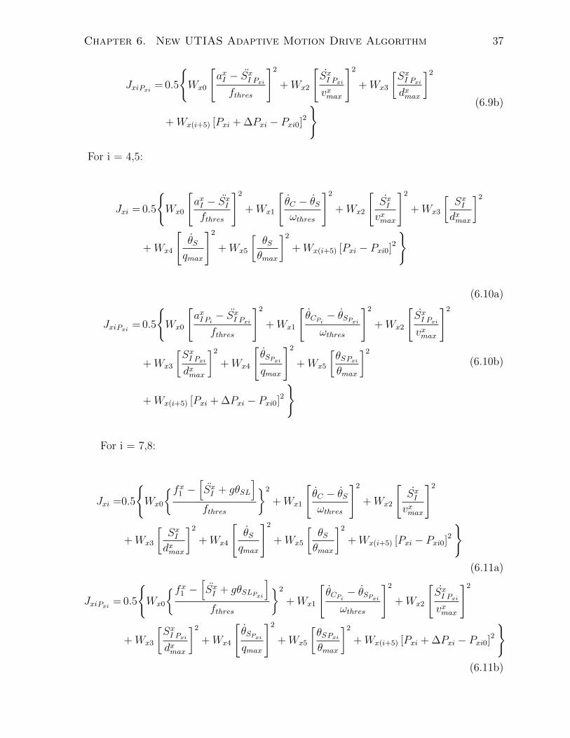
Chapter 6. New UTIAS Adaptive Motion Drive Algorithm 37
JxiPxi = 0.5
Wx0
[axI − SxI Pxifthres
]2
+Wx2
[SxI Pxivxmax
]2
+Wx3
[SxI Pxidxmax
]2
+Wx(i+5) [Pxi + ∆Pxi − Pxi0]2 (6.9b)
For i = 4,5:
Jxi = 0.5
Wx0
[axI − SxIfthres
]2
+Wx1
[θC − θSωthres
]2
+Wx2
[SxIvxmax
]2
+Wx3
[SxIdxmax
]2
+Wx4
[θSqmax
]2
+Wx5
[θSθmax
]2
+Wx(i+5) [Pxi − Pxi0]2
(6.10a)
JxiPxi = 0.5
Wx0
[axI Pi − S
xI Pxi
fthres
]2
+Wx1
[θCPi − θSPxi
ωthres
]2
+Wx2
[SxI Pxivxmax
]2
+Wx3
[SxI Pxidxmax
]2
+Wx4
[θSPxiqmax
]2
+Wx5
[θSPxiθmax
]2
+Wx(i+5) [Pxi + ∆Pxi − Pxi0]2 (6.10b)
For i = 7,8:
Jxi =0.5
Wx0
fx1 − [SxI + gθSL
]fthres
2
+Wx1
[θC − θSωthres
]2
+Wx2
[SxIvxmax
]2
+Wx3
[SxIdxmax
]2
+Wx4
[θSqmax
]2
+Wx5
[θSθmax
]2
+Wx(i+5) [Pxi − Pxi0]2
(6.11a)
JxiPxi = 0.5
Wx0
fx1 − [SxI + gθSLPxi
]fthres
2
+Wx1
[θCPi − θSPxi
ωthres
]2
+Wx2
[SxI Pxivxmax
]2
+Wx3
[SxI Pxidxmax
]2
+Wx4
[θSPxiqmax
]2
+Wx5
[θSPxiθmax
]2
+Wx(i+5) [Pxi + ∆Pxi − Pxi0]2
(6.11b)
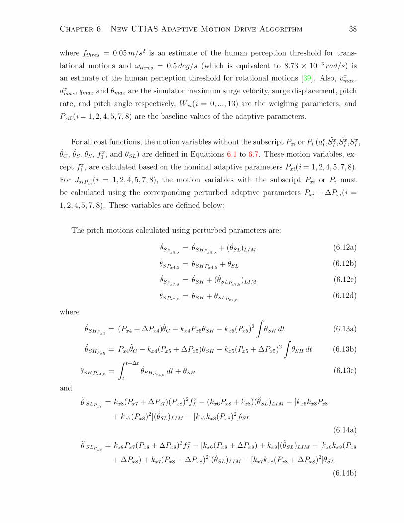
Chapter 6. New UTIAS Adaptive Motion Drive Algorithm 38
where fthres = 0.05m/s2 is an estimate of the human perception threshold for trans-
lational motions and ωthres = 0.5 deg/s (which is equivalent to 8.73 × 10⁻³ rad/s) is
an estimate of the human perception threshold for rotational motions [39]. Also, vxmax,
dxmax, qmax and θmax are the simulator maximum surge velocity, surge displacement, pitch
rate, and pitch angle respectively, Wxi(i = 0, ..., 13) are the weighing parameters, and
Pxi0(i = 1, 2, 4, 5, 7, 8) are the baseline values of the adaptive parameters.
For all cost functions, the motion variables without the subscript Pxi or Pi (axI ,SxI ,SxI ,SxI ,
θC , θS, θS, fx1 , and θSL) are defined in Equations 6.1 to 6.7. These motion variables, ex-
cept fx1 , are calculated based on the nominal adaptive parameters Pxi(i = 1, 2, 4, 5, 7, 8).
For JxiPxi(i = 1, 2, 4, 5, 7, 8), the motion variables with the subscript Pxi or Pi must
be calculated using the corresponding perturbed adaptive parameters Pxi + ∆Pxi(i =
1, 2, 4, 5, 7, 8). These variables are defined below:
The pitch motions calculated using perturbed parameters are:
θSPx4,5 = θSHPx4,5 + (θSL)LIM (6.12a)
θSPx4,5 = θSHPx4,5 + θSL (6.12b)
θSPx7,8 = θSH + (θSLPx7,8 )LIM (6.12c)
θSPx7,8 = θSH + θSLPx7,8 (6.12d)
where
θSHPx4 = (Px4 + ∆Px4)θC − kx4Px5θSH − kx5(Px5)2
∫θSH dt (6.13a)
θSHPx5 = Px4θC − kx4(Px5 + ∆Px5)θSH − kx5(Px5 + ∆Px5)2
∫θSH dt (6.13b)
θSHPx4,5 =
∫ t+∆t
t
θSHPx4,5 dt+ θSH (6.13c)
and...θ SLPx7 = kx8(Px7 + ∆Px7)(Px8)2fxL − (kx6Px8 + kx8)(θSL)LIM − [kx6kx8Px8
+ kx7(Px8)2](θSL)LIM − [kx7kx8(Px8)2]θSL
(6.14a)...θ SLPx8 = kx8Px7(Px8 + ∆Px8)2fxL − [kx6(Px8 + ∆Px8) + kx8](θSL)LIM − [kx6kx8(Px8
+ ∆Px8) + kx7(Px8 + ∆Px8)2](θSL)LIM − [kx7kx8(Px8 + ∆Px8)2]θSL
(6.14b)
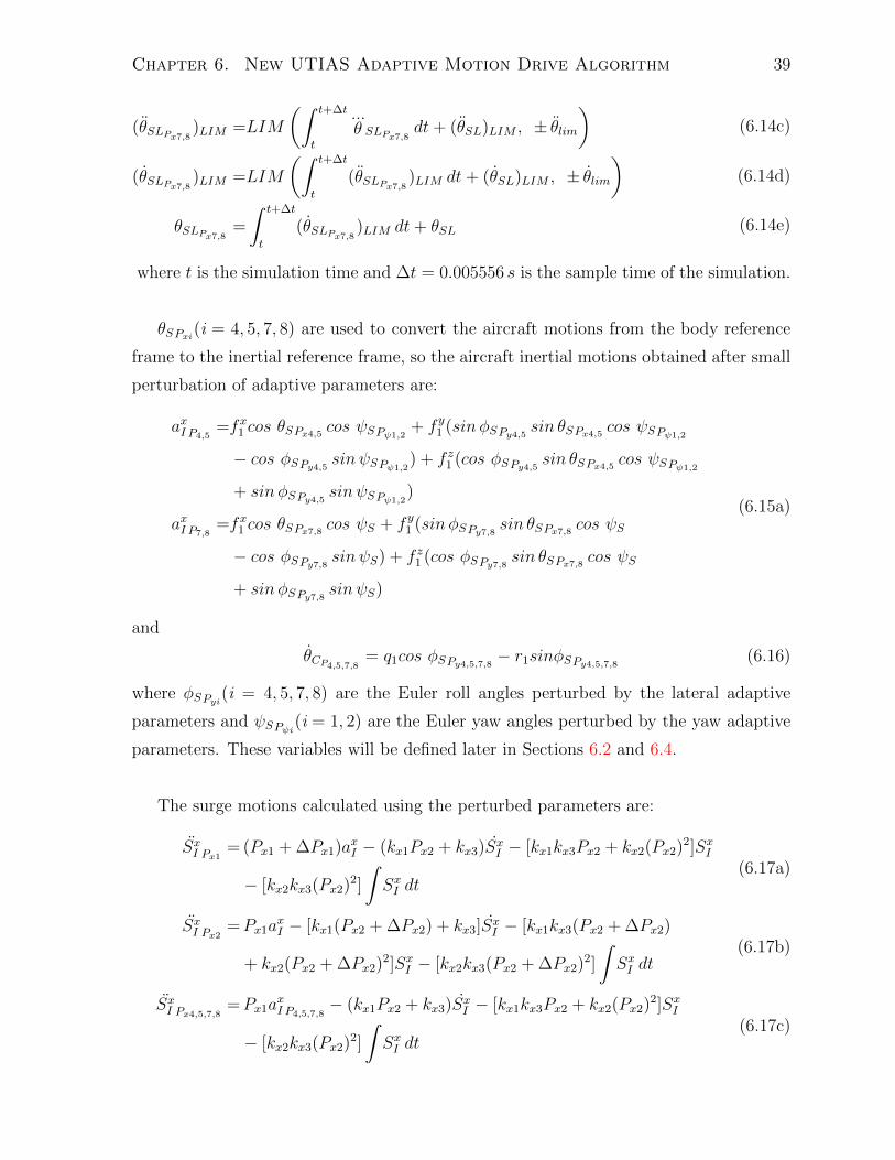
Chapter 6. New UTIAS Adaptive Motion Drive Algorithm 39
(θSLPx7,8 )LIM =LIM
(∫ t+∆t
t
...θ SLPx7,8 dt+ (θSL)LIM , ± θlim
)(6.14c)
(θSLPx7,8 )LIM =LIM
(∫ t+∆t
t
(θSLPx7,8 )LIM dt+ (θSL)LIM , ± θlim)
(6.14d)
θSLPx7,8 =
∫ t+∆t
t
(θSLPx7,8 )LIM dt+ θSL (6.14e)
where t is the simulation time and ∆t = 0.005556 s is the sample time of the simulation.
θSPxi(i = 4, 5, 7, 8) are used to convert the aircraft motions from the body reference
frame to the inertial reference frame, so the aircraft inertial motions obtained after small
perturbation of adaptive parameters are:
axI P4,5=fx1 cos θSPx4,5 cos ψSPψ1,2
+ f y1 (sin φSPy4,5 sin θSPx4,5 cos ψSPψ1,2
− cos φSPy4,5 sinψSPψ1,2) + f z1 (cos φSPy4,5 sin θSPx4,5 cos ψSPψ1,2
+ sin φSPy4,5 sinψSPψ1,2)
axI P7,8=fx1 cos θSPx7,8 cos ψS + f y1 (sin φSPy7,8 sin θSPx7,8 cos ψS
− cos φSPy7,8 sinψS) + f z1 (cos φSPy7,8 sin θSPx7,8 cos ψS
+ sin φSPy7,8 sinψS)
(6.15a)
and
θCP4,5,7,8 = q1cos φSPy4,5,7,8 − r1sinφSPy4,5,7,8 (6.16)
where φSPyi(i = 4, 5, 7, 8) are the Euler roll angles perturbed by the lateral adaptive
parameters and ψSPψi(i = 1, 2) are the Euler yaw angles perturbed by the yaw adaptive
parameters. These variables will be defined later in Sections 6.2 and 6.4.
The surge motions calculated using the perturbed parameters are:
SxI Px1 = (Px1 + ∆Px1)axI − (kx1Px2 + kx3)SxI − [kx1kx3Px2 + kx2(Px2)2]SxI
− [kx2kx3(Px2)2]
∫SxI dt
(6.17a)
SxI Px2 =Px1axI − [kx1(Px2 + ∆Px2) + kx3]SxI − [kx1kx3(Px2 + ∆Px2)
+ kx2(Px2 + ∆Px2)2]SxI − [kx2kx3(Px2 + ∆Px2)2]
∫SxI dt
(6.17b)
SxI Px4,5,7,8 =Px1axI P4,5,7,8
− (kx1Px2 + kx3)SxI − [kx1kx3Px2 + kx2(Px2)2]SxI
− [kx2kx3(Px2)2]
∫SxI dt
(6.17c)
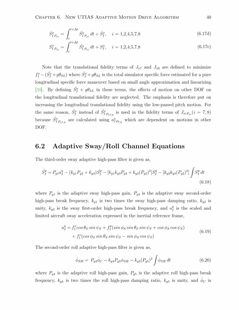
Chapter 6. New UTIAS Adaptive Motion Drive Algorithm 40
SxI Pxi =
∫ t+∆t
t
SxI Pxi dt+ SxI , i = 1,2,4,5,7,8 (6.17d)
SxI Pxi =
∫ t+∆t
t
SxI Pxi dt+ SxI , i = 1,2,4,5,7,8 (6.17e)
Note that the translational fidelity terms of Jx7 and Jx8 are defined to minimize
fx1 − (SxI +gθSL) where SxI +gθSL is the total simulator specific force estimated for a pure
longitudinal specific force maneuver based on small angle approximation and linearizing
[30]. By defining SxI + gθSL in these terms, the effects of motion on other DOF on
the longitudinal translational fidelity are neglected. The emphasis is therefore put on
increasing the longitudinal translational fidelity using the low-passed pitch motion. For
the same reason, SxI instead of SxI Px7,8 is used in the fidelity terms of JxiPxi(i = 7, 8)
because SxI Px7,8 are calculated using axI P7,8which are dependent on motions in other
DOF.
6.2 Adaptive Sway/Roll Channel Equations
The third-order sway adaptive high-pass filter is given as,
SyI =Py1ayI − (ky1Py2 + ky3)SyI − [ky1ky3Py2 + ky2(Py2)2]SyI − [ky2ky3(Py2)2]
∫SyI dt
(6.18)
where Py1 is the adaptive sway high-pass gain, Py2 is the adaptive sway second-order
high-pass break frequency, ky1 is two times the sway high-pass damping ratio, ky2 is
unity, ky3 is the sway first-order high-pass break frequency, and ayI is the scaled and
limited aircraft sway acceleration expressed in the inertial reference frame,
ayI = fx1 cos θS sinψS + f y1 (sin φS sin θS sinψS + cos φS cos ψS)
+ f z1 (cos φS sin θS sinψS − sin φS cos ψS)(6.19)
The second-order roll adaptive high-pass filter is given as,
φSH = Py4φC − ky4Py5φSH − ky5(Py5)2
∫φSH dt (6.20)
where Py4 is the adaptive roll high-pass gain, Py5 is the adaptive roll high-pass break
frequency, ky4 is two times the roll high-pass damping ratio, ky5 is unity, and φC is
Chapter 6. New UTIAS Adaptive Motion Drive Algorithm 41
calculated by converting the scaled and limited body rates of the aircraft into the Euler
rates of the simulator,
φC = p1 + (q1sin φS + r1cos φS)tan θS (6.21)
The third-order sway low-pass filter is given as,
...φSL = ky8Py7(Py8)2f yL − (ky6Py8 + ky8)(φSL)LIM − [ky6ky8Py8
+ ky7(Py8)2](φSL)LIM − [ky7ky8(Py8)2]φSL(6.22a)
(φSL)LIM =LIM
(∫...φSL dt, ± φlim
)(6.22b)
(φSL)LIM =LIM
(∫(φSL)LIM dt, ± φlim
)(6.22c)
φSL =
∫(φSL)LIM dt (6.22d)
where Py7 is the adaptive sway low-pass gain, Py8 is the adaptive sway second-order low-
pass break frequency, ky6 is two times the sway low-pass damping ratio, ky7 is unity, ky8
is the sway first-order low-pass break frequency, φlim = 100 rad/s2 is the tilt-acceleration
limit for roll motion, φlim = 0.0698 rad/s is the tilt-rate limit for roll motion, and f yL is
the lateral specific force due to tilt coordination,
f yL = −fy1
g(6.23)
Using Equations 6.20 and 6.22, the total simulator roll motions can be calculated as
φS = φSH + (φSL)LIM (6.24)
The sway/roll parameter adaptation rates are defined as
Pyi = −Gyi∂Jyi∂Pyi
, i = 1,2,4,5,7,8
= −Gyi
lim
∆Pyi→0
[Jyi(Pyi + ∆Pyi)− Jyi(Pyi)
∆Pyi
]= −Gyi
[lim
∆Pyi→0
(JyiPyi − Jyi
∆Pyi
)]
≈ −Gyi
(JyiPyi − Jyi
∆Pyi
)if ∆Pyi 1
(6.25)
where Gyi are the step sizes. The cost functions are:
Chapter 6. New UTIAS Adaptive Motion Drive Algorithm 42
For i = 1,2:
Jyi = 0.5
Wy0
[ayI − S
yI
fthres
]2
+Wy2
[SyIvymax
]2
+Wy3
[SyIdymax
]2
+Wy(i+5) [Pyi − Pyi0]2 (6.26a)
JyiPyi = 0.5
Wy0
[ayI − S
yI Pyi
fthres
]2
+Wy2
[SyI Pyivymax
]2
+Wy3
[SyI Pyidymax
]2
+Wy(i+5) [Pyi + ∆Pyi − Pyi0]2 (6.26b)
For i = 4,5:
Jyi = 0.5
Wy0
[ayI − S
yI
fthres
]2
+Wy1
[φC − φSωthres
]2
+Wy2
[SyIvymax
]2
+Wy3
[SyIdymax
]2
+Wy4
[φSpmax
]2
+Wy5
[φSφmax
]2
+Wy(i+5) [Pyi − Pyi0]2
(6.27a)
JyiPyi = 0.5
Wy0
[ayIPi − S
yI Pyi
fthres
]2
+Wy1
[φCPi − φSPyi
ωthres
]2
+Wy2
[SyI Pyivymax
]2
+Wy3
[SyI Pyidymax
]2
+Wy4
[φSPyipmax
]2
+Wy5
[φSPyiφmax
]2
+Wy(i+5) [Pyi + ∆Pyi − Pyi0]2
(6.27b)
For i = 7,8:
Jyi =0.5
Wy0
f y1 − [SyI − gφSL]fthres
2
+Wy1
[φC − φSωthres
]2
+Wy2
[SyIvymax
]2
+Wy3
[SyIdymax
]2
+Wy4
[φSpmax
]2
+Wy5
[φSφmax
]2
+Wy(i+5) [Pyi − Pyi0]2
(6.28a)
Chapter 6. New UTIAS Adaptive Motion Drive Algorithm 43
JyiPyi = 0.5
Wy0
f y1 − [SyI − gφSLPyi]fthres
2
+Wy1
[φCPi − φSPyi
ωthres
]2
+Wy2
[SyI Pyivymax
]2
+Wy3
[SyI Pyidymax
]2
+Wy4
[φSPyipmax
]2
+Wy5
[φSPyiφmax
]2
+Wy(i+5) [Pyi + ∆Pyi − Pyi0]2
(6.28b)
where vymax, dymax, pmax and φmax are the simulator maximum sway velocity, sway displace-
ment, roll rate, and roll angle respectively, Wyi(i = 0, ..., 13) are the weighing parameters,
and Pyi0(i = 1, 2, 4, 5, 7, 8) are the baseline values of the adaptive parameters.
For all cost functions, the motion variables without the subscript Pyi or Pi (ayI ,SyI ,SyI ,SyI ,
φC , φS, φS, f y1 , and φSL) are defined in Equations 6.18 to 6.24. These motion variables, ex-
cept f y1 , are calculated based on the nominal adaptive parameters Pyi(i = 1, 2, 4, 5, 7, 8).
For JyiPyi(i = 1, 2, 4, 5, 7, 8), the motion variables with the subscript Pyi or Pi must
be calculated using the corresponding perturbed adaptive parameters Pyi + ∆Pyi(i =
1, 2, 4, 5, 7, 8). These variables are defined below:
The roll motions calculated using perturbed parameters are:
φSPy4,5 = φSHPy4,5 + (φSL)LIM (6.29a)
φSPy4,5 = φSHPy4,5 + φSL (6.29b)
φSPy7,8 = φSH + (φSLPy7,8 )LIM (6.29c)
φSPy7,8 = φSH + φSLPy7,8 (6.29d)
where
φSHPy4 = (Py4 + ∆Py4)φC − ky4Py5φSH − ky5(Py5)2
∫φSH dt (6.30a)
φSHPy5 = Py4φC − ky4(Py5 + ∆Py5)φSH − ky5(Py5 + ∆Py5)2
∫φSH dt (6.30b)
φSHPy4,5 =
∫ t+∆t
t
φSHPy4,5 dt+ φSH (6.30c)
and...φSLPy7 = ky8(Py7 + ∆Py7)(Py8)2f yL − (ky6Py8 + ky8)(φSL)LIM − [ky6ky8Py8
+ ky7(Py8)2](φSL)LIM − [ky7ky8(Py8)2]φSL
(6.31a)
Chapter 6. New UTIAS Adaptive Motion Drive Algorithm 44
...φSLPy8 = ky8Py7(Py8 + ∆Py8)2f yL − [ky6(Py8 + ∆Py8) + ky8](φSL)LIM − [ky6ky8(Py8
+ ∆Py8) + ky7(Py8 + ∆Py8)2](φSL)LIM − [ky7ky8(Py8 + ∆Py8)2]φSL
(6.31b)
(φSLPy7,8 )LIM =LIM
(∫ t+∆t
t
...φSLPy7,8 dt+ (φSL)LIM , ± φlim
)(6.31c)
(φSLPy7,8 )LIM =LIM
(∫ t+∆t
t
(φSLPy7,8 )LIM dt+ (φSL)LIM , ± φlim)
(6.31d)
φSLPy7,8 =
∫ t+∆t
t
(φSLPy7,8 )LIM dt+ φSL (6.31e)
φSPyi(i = 4, 5, 7, 8) are used to convert the aircraft motions from the body reference
frame to the inertial reference frame, so the aircraft inertial motions obtained after small
perturbation of adaptive parameters are:
ayIP4,5=fx1 cos θSPx4,5 sinψSPψ1,2
+ f y1 (sin φSPy4,5 sin θSPx4,5 sinψSPψ1,2
+ cos φSPy4,5 cos ψSPψ1,2) + f z1 (cos φSPy4,5 sin θSPx4,5 sinψSPψ1,2
− sin φSPy4,5 cos ψSPψ1,2)
(6.32a)
ayIP7,8=fx1 cos θSPx7,8 sinψS + f y1 (sin φSPy7,8 sin θSPx7,8 sinψS
+ cos φSPy7,8 cos ψS) + f z1 (cos φSPy7,8 sin θSPx7,8 sinψS
− sin φSPy7,8 cos ψS)
(6.32b)
and
φCP4,5,7,8 = p1 + (q1sin φSPy4,5,7,8 + r1cos φSPy4,5,7,8)tan θSPx4,5,7,8 (6.33)
The sway motions calculated using the perturbed parameters are:
SyI Py1 = (Py1 + ∆Py1)ayI − (ky1Py2 + ky3)SyI − [ky1ky3Py2 + ky2(Py2)2]SyI
− [ky2ky3(Py2)2]
∫SyI dt
(6.34a)
SyI Py2 =Py1ayI − [ky1(Py2 + ∆Py2) + ky3]SyI − [ky1ky3(Py2 + ∆Py2)
+ ky2(Py2 + ∆Py2)2]SyI − [ky2ky3(Py2 + ∆Py2)2]
∫SyI dt
(6.34b)
SyI Py4,5,7,8 =Py1ayIP4,5,7,8
− (ky1Py2 + ky3)SyI − [ky1ky3Py2 + ky2(Py2)2]SyI
− [ky2ky3(Py2)2]
∫SyI dt
(6.34c)
Chapter 6. New UTIAS Adaptive Motion Drive Algorithm 45
SyI Pyi =
∫ t+∆t
t
SyI Pyi dt+ SyI , i = 1,2,4,5,7,8 (6.34d)
SyI Pyi =
∫ t+∆t
t
SyI Pyi dt+ SyI , i = 1,2,4,5,7,8 (6.34e)
Note that the translational fidelity terms of Jy7 and Jy8 are defined to minimize
f y1 − (SyI − gφSL) where SyI − gφSL is the total simulator specific force estimated for a
pure lateral specific force maneuver based on small angle approximation and linearizing
[30]. By defining SyI − gφSL in these terms, the effects of motion on other DOF on the
lateral translational fidelity are neglected. The emphasis is therefore put on increasing
the lateral translational fidelity using the low-passed roll motion. For the same reason,
SyI instead of SyI Py7,8 is used in the fidelity terms of JyiPyi(i = 7, 8) because SyI Py7,8 are
calculated using ayIP7,8which are dependent on motions in other DOF.
6.3 Adaptive Heave Channel Equations
The third-order heave adaptive high-pass filter is given as,
SzI =Pz1azI − (kz1Pz2 + kz3)SzI − [kz1kz3Pz2 + kz2(Pz2)2]SzI − [kz2kz3(Pz2)2]
∫SzI dt
(6.35)
where Pz1 is the adaptive heave high-pass gain, Pz2 is the adaptive heave second-order
high-pass break frequency, kz1 is two times the heave high-pass damping ratio, kz2 is
unity, kz3 is the heave first-order high-pass break frequency, and azI is the scaled and
limited aircraft heave acceleration expressed in the inertial reference frame,
azI =− fx1 sin θS + f y1 sin φS cos θS + f z1 cos φS cos θS + g (6.36)
The heave parameter adaptation rates are
Pzi = −Gzi∂Jzi∂Pzi
, i = 1,2
= −Gzi
lim
∆Pzi→0
[Jzi(Pzi + ∆Pzi)− Jzi(Pzi)
∆Pzi
]= −Gzi
[lim
∆Pzi→0
(JziPzi − Jzi
∆Pzi
)]≈ −Gzi
(JziPzi − Jzi
∆Pzi
)if ∆Pzi 1
(6.37)
Chapter 6. New UTIAS Adaptive Motion Drive Algorithm 46
where Gzi are the step sizes. The cost functions are given by
Jzi = 0.5
Wz0
[azI − SzIfthres
]2
+Wz1
[SzIvzmax
]2
+Wz2
[SzIdzmax
]2
+Wz(i+2)[Pzi − Pzi0]2
(6.38a)
JziPzi = 0.5
Wz0
[azI − SzI Pzifthres
]2
+Wz1
[SzI Pzivzmax
]2
+Wz2
[SzI Pzidzmax
]2
+Wz(i+2) [Pzi + ∆Pzi − Pzi0]2 (6.38b)
where i=1,2, vzmax and dzmax are the simulator maximum heave velocity and heave dis-
placement respectively, Wzi(i = 0, ..., 4) are the weighing parameters, and Pzi0(i = 1, 2)
are the baseline values of the adaptive parameters.
For all cost functions, the motion variables azI , SzI , SzI , and SzI are calculated using
the nominal adaptive parameters Pzi(i = 1, 2). These variables are defined in Equations
6.35 to 6.36. For JziPzi(i = 1, 2), the motion variables with the subscript Pzi must be
calculated using the corresponding perturbed adaptive parameter Pzi + ∆Pzi(i = 1, 2).
These variables are defined below:
SzI Pz1 = (Pz1 + ∆Pz1)azI − (kz1Pz2 + kz3)SzI − [kz1kz3Pz2 + kz2(Pz2)2]SzI
− [kz2kz3(Pz2)2]
∫SzI dt
(6.39a)
SzI Pz2 =Pz1azI − [kz1(Pz2 + ∆Pz2) + kz3]SzI − [kz1kz3(Pz2 + ∆Pz2)
+ kz2(Pz2 + ∆Pz2)2]SzI − [kz2kz3(Pz2 + ∆Pz2)2]
∫SzI dt
(6.39b)
SzI Pzi =
∫ t+∆t
t
SzI Pzi dt+ SzI , i = 1,2 (6.39c)
SzI Pzi =
∫ t+∆t
t
SzI Pzi dt+ SzI , i = 1,2 (6.39d)
6.4 Adaptive Yaw Channel Equations
The second-order yaw adaptive high-pass filter is given as,
ψS = ψSH
=Pψ1ψC − kψ1Pψ2ψSH − kψ2(Pψ2)2
∫ψSH dt
(6.40)
Chapter 6. New UTIAS Adaptive Motion Drive Algorithm 47
where Pψ1 is the adaptive yaw high-pass gain, Pψ2 is the adaptive yaw high-pass break
frequency, kψ1 is two times the yaw high-pass damping ratio, kψ2 is unity and ψC is
calculated by converting the scaled and limited body rates of the aircraft into the Euler
rates of the simulator,
ψC = (q1sin φS + r1cos φS)sec θS (6.41)
The yaw parameter adaptation rates are
Pψi = −Gψi∂Jψi∂Pψi
, i = 1,2
= −Gψi
lim
∆Pψi→0
[Jψi(Pψi + ∆Pψi)− Jψi(Pψi)
∆Pψi
]= −Gψi
[lim
∆Pψi→0
(JψiPψi − Jψi
∆Pψi
)]
≈ −Gψi
(JψiPψi − Jψi
∆Pψi
)if ∆Pψi 1
(6.42)
where Gψi are the step sizes. The cost functions are given by
Jψi =0.5
Wψ0
[ψC − ψSωthres
]2
+Wψ1
[ψSrmax
]2
+Wψ2
[ψSψmax
]2
+Wψ(i+2) [Pψi − Pψi0]2 (6.43a)
JψiPψi =0.5
Wψ0
[ψCP(i+3)
− ψSPψiωthres
]2
+Wψ1
[ψSPψirmax
]2
+Wψ2
[ψSPψiψmax
]2
+Wψ(i+2) [Pψi + ∆Pψi − Pψi0]2 (6.43b)
where i=1,2, rmax and ψmax are the simulator maximum yaw rate, and yaw angle respec-
tively, Wψi(i = 0, ..., 4) are the weighing parameters, and Pψi0(i = 1, 2) are the baseline
values of the adaptive parameters.
For all cost functions, the motion variables ψC , ψS, and ψS are calculated using the
nominal adaptive parameter Pψi(i = 1, 2). These variables are defined in Equations 6.40
to 6.41. For JψiPψi(i = 1, 2), the motion variables with the subscript Pψi or P(i+3) must be
calculated using the corresponding perturbed adaptive parameters Pψi + ∆Pψi(i = 1, 2)
Chapter 6. New UTIAS Adaptive Motion Drive Algorithm 48
as defined below:
ψSPψ1=ψSHPψ1
= (Pψ1 + ∆Pψ1)ψC − kψ1Pψ2ψSH − kψ2(Pψ2)2
∫ψSH dt
(6.44a)
ψSPψ2=ψSHPψ2
=Pψ1ψC − kψ1(Pψ2 + ∆Pψ2)ψSH − kψ2(Pψ2 + ∆Pψ2)2
∫ψSH dt
(6.44b)
ψSPψi =ψSHPψi , i = 1,2
=
∫ t+∆t
t
ψSHPψi dt+ ψSH(6.44c)
and
ψCPi = (q1sin φSPyi + r1cos φSPyi)sec θSPxi , i = 4,5 (6.45a)
6.5 A Comparison between the Original and the New
Adaptive MDA
A desktop simulation was conducted to compare the performance of the new (numeri-
cal) adaptive MDA to the performance of the original (analytical) adaptive MDA. The
comparison was based on the simulation of a surge acceleration step input of 10m/s2.
Similar to the study performed by O’Toole [37], the performance of the two MDAs was
investigated by examining the adaptation of the surge filter gain (Px1) using the cost
function translational fidelity term. By employing the surge high-pass filter parameters
listed in Table A.5 in Appendix A.2, the surge acceleration step input was first simulated
at 180Hz three times using the original MDA, each time with a different value assigned
to the surge fidelity weight (Wx0). Next, the same simulation was repeated using the new
MDA where the identical set of filter parameters was employed. The simulation results
produced by the original and the new algorithm are presented in Figures 6.2 and 6.3
respectively. As shown in Figure 6.2, the simulator response generated using the original
MDA reached a steady state of zero shortly after the start of the simulation without
properly minimizing the difference between the aircraft and the simulator acceleration.
This result is in agreement with the findings of O’Toole [37]. Moreover, it is depicted
in Figure 6.2 that the value of Wx0 had no positive effects on the improvement of the
simulator fidelity. In contrast, the new algorithm successfully maximized the simulator
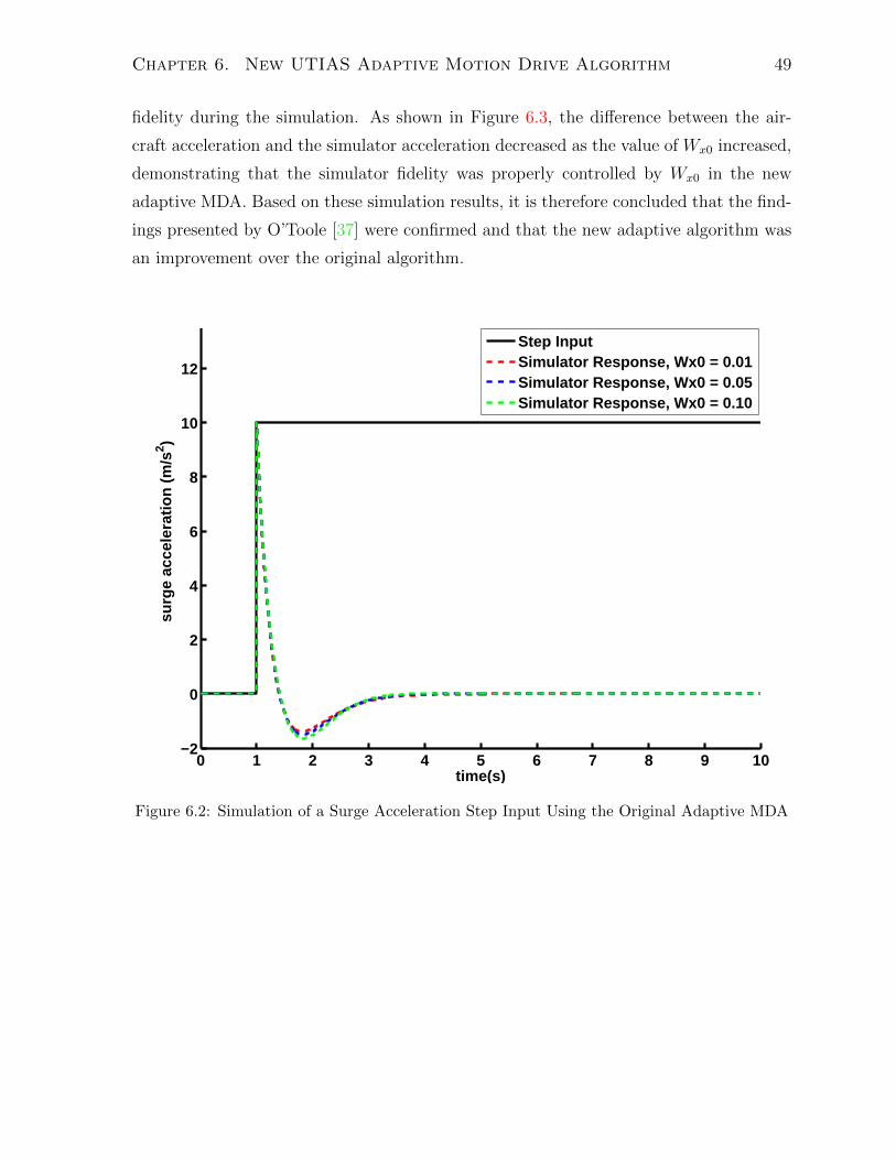
Chapter 6. New UTIAS Adaptive Motion Drive Algorithm 49
fidelity during the simulation. As shown in Figure 6.3, the difference between the air-
craft acceleration and the simulator acceleration decreased as the value of Wx0 increased,
demonstrating that the simulator fidelity was properly controlled by Wx0 in the new
adaptive MDA. Based on these simulation results, it is therefore concluded that the find-
ings presented by O’Toole [37] were confirmed and that the new adaptive algorithm was
an improvement over the original algorithm.
0 1 2 3 4 5 6 7 8 9 10−2
0
2
4
6
8
10
12
time(s)
surg
e ac
cele
rati
on
(m
/s2 )
Step InputSimulator Response, Wx0 = 0.01Simulator Response, Wx0 = 0.05Simulator Response, Wx0 = 0.10
Figure 6.2: Simulation of a Surge Acceleration Step Input Using the Original Adaptive MDA
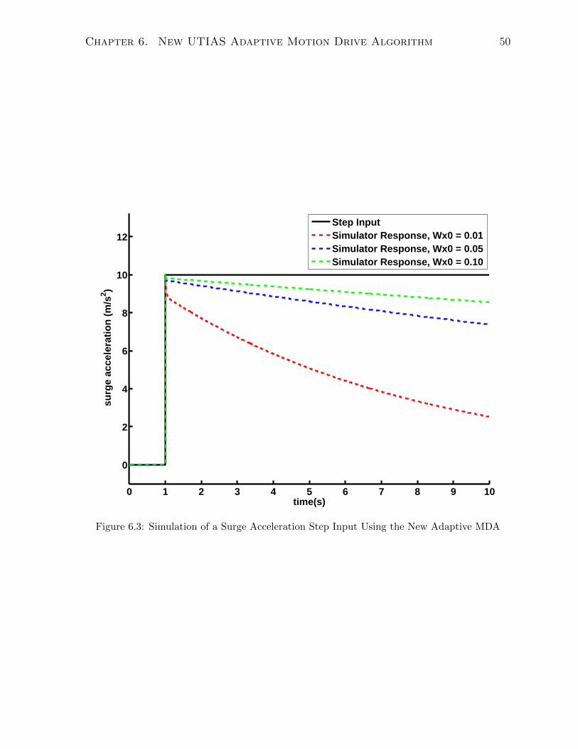
Chapter 6. New UTIAS Adaptive Motion Drive Algorithm 50
0 1 2 3 4 5 6 7 8 9 10
0
2
4
6
8
10
12
time(s)
surg
e ac
cele
rati
on
(m
/s2 )
Step InputSimulator Response, Wx0 = 0.01Simulator Response, Wx0 = 0.05Simulator Response, Wx0 = 0.10
Figure 6.3: Simulation of a Surge Acceleration Step Input Using the New Adaptive MDA
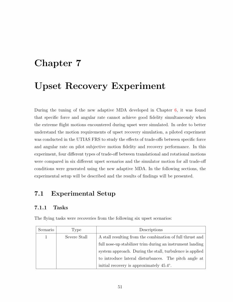
Chapter 7
Upset Recovery Experiment
During the tuning of the new adaptive MDA developed in Chapter 6, it was found
that specific force and angular rate cannot achieve good fidelity simultaneously when
the extreme flight motions encountered during upset were simulated. In order to better
understand the motion requirements of upset recovery simulation, a piloted experiment
was conducted in the UTIAS FRS to study the effects of trade-offs between specific force
and angular rate on pilot subjective motion fidelity and recovery performance. In this
experiment, four different types of trade-off between translational and rotational motions
were compared in six different upset scenarios and the simulator motion for all trade-off
conditions were generated using the new adaptive MDA. In the following sections, the
experimental setup will be described and the results of findings will be presented.
7.1 Experimental Setup
7.1.1 Tasks
The flying tasks were recoveries from the following six upset scenarios:
Scenario Type Descriptions
1 Severe Stall A stall resulting from the combination of full thrust and
full nose-up stabilizer trim during an instrument landing
system approach. During the stall, turbulence is applied
to introduce lateral disturbances. The pitch angle at
initial recovery is approximately 45.4.
51
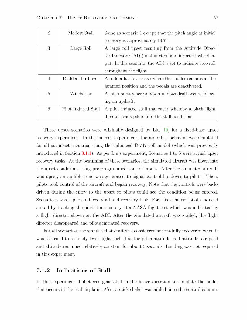
Chapter 7. Upset Recovery Experiment 52
2 Modest Stall Same as scenario 1 except that the pitch angle at initial
recovery is approximately 19.7.
3 Large Roll A large roll upset resulting from the Attitude Direc-
tor Indicator (ADI) malfunction and incorrect wheel in-
put. In this scenario, the ADI is set to indicate zero roll
throughout the flight.
4 Rudder Hard-over A rudder hardover case where the rudder remains at the
jammed position and the pedals are deactivated.
5 Windshear A microburst where a powerful downdraft occurs follow-
ing an updraft.
6 Pilot Induced Stall A pilot induced stall maneuver whereby a pitch flight
director leads pilots into the stall condition.
These upset scenarios were originally designed by Liu [10] for a fixed-base upset
recovery experiment. In the current experiment, the aircraft’s behavior was simulated
for all six upset scenarios using the enhanced B-747 roll model (which was previously
introduced in Section 3.1.1). As per Liu’s experiment, Scenarios 1 to 5 were actual upset
recovery tasks. At the beginning of these scenarios, the simulated aircraft was flown into
the upset conditions using pre-programmed control inputs. After the simulated aircraft
was upset, an audible tone was generated to signal control handover to pilots. Then,
pilots took control of the aircraft and began recovery. Note that the controls were back-
driven during the entry to the upset so pilots could see the condition being entered.
Scenario 6 was a pilot induced stall and recovery task. For this scenario, pilots induced
a stall by tracking the pitch time history of a NASA flight test which was indicated by
a flight director shown on the ADI. After the simulated aircraft was stalled, the flight
director disappeared and pilots initiated recovery.
For all scenarios, the simulated aircraft was considered successfully recovered when it
was returned to a steady level flight such that the pitch attitude, roll attitude, airspeed
and altitude remained relatively constant for about 5 seconds. Landing was not required
in this experiment.
7.1.2 Indications of Stall
In this experiment, buffet was generated in the heave direction to simulate the buffet
that occurs in the real airplane. Also, a stick shaker was added onto the control column.
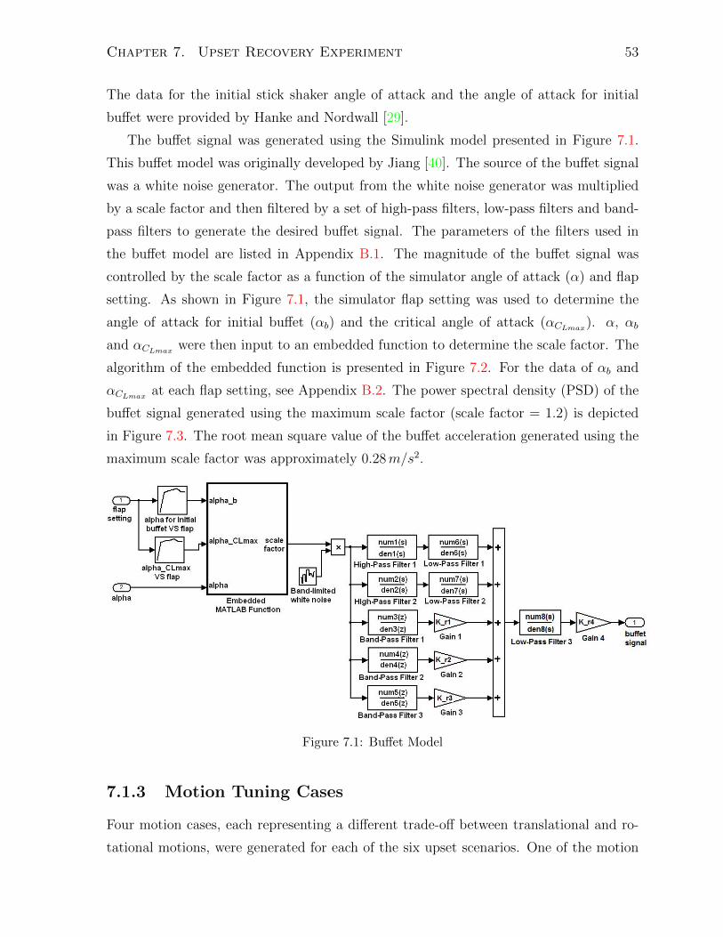
Chapter 7. Upset Recovery Experiment 53
The data for the initial stick shaker angle of attack and the angle of attack for initial
buffet were provided by Hanke and Nordwall [29].
The buffet signal was generated using the Simulink model presented in Figure 7.1.
This buffet model was originally developed by Jiang [40]. The source of the buffet signal
was a white noise generator. The output from the white noise generator was multiplied
by a scale factor and then filtered by a set of high-pass filters, low-pass filters and band-
pass filters to generate the desired buffet signal. The parameters of the filters used in
the buffet model are listed in Appendix B.1. The magnitude of the buffet signal was
controlled by the scale factor as a function of the simulator angle of attack (α) and flap
setting. As shown in Figure 7.1, the simulator flap setting was used to determine the
angle of attack for initial buffet (αb) and the critical angle of attack (αCLmax). α, αb
and αCLmax were then input to an embedded function to determine the scale factor. The
algorithm of the embedded function is presented in Figure 7.2. For the data of αb and
αCLmax at each flap setting, see Appendix B.2. The power spectral density (PSD) of the
buffet signal generated using the maximum scale factor (scale factor = 1.2) is depicted
in Figure 7.3. The root mean square value of the buffet acceleration generated using the
maximum scale factor was approximately 0.28m/s2.
Figure 7.1: Buffet Model
7.1.3 Motion Tuning Cases
Four motion cases, each representing a different trade-off between translational and ro-
tational motions, were generated for each of the six upset scenarios. One of the motion
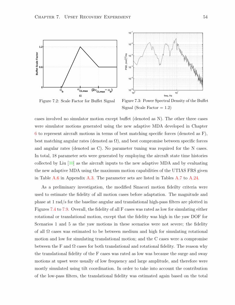
Chapter 7. Upset Recovery Experiment 54
0
0.6
1.2
α
Bu
ffet
Sca
le F
acto
r
αb
αCLmax (2α
CLmax− α
b)
Figure 7.2: Scale Factor for Buffet Signal
100 10110−6
10−5
10−4
10−3
10−2
10−1
freq, Hz
PSD
, (m
/s2 )2 /Hz
Figure 7.3: Power Spectral Density of the Buffet
Signal (Scale Factor = 1.2)
cases involved no simulator motion except buffet (denoted as N). The other three cases
were simulator motions generated using the new adaptive MDA developed in Chapter
6 to represent aircraft motions in terms of best matching specific forces (denoted as F),
best matching angular rates (denoted as Ω), and best compromise between specific forces
and angular rates (denoted as C). No parameter tuning was required for the N cases.
In total, 18 parameter sets were generated by employing the aircraft state time histories
collected by Liu [10] as the aircraft inputs to the new adaptive MDA and by evaluating
the new adaptive MDA using the maximum motion capabilities of the UTIAS FRS given
in Table A.6 in Appendix A.3. The parameter sets are listed in Tables A.7 to A.24.
As a preliminary investigation, the modified Sinacori motion fideilty criteria were
used to estimate the fidelity of all motion cases before adaptation. The magnitude and
phase at 1 rad/s for the baseline angular and translational high-pass filters are plotted in
Figures 7.4 to 7.9. Overall, the fidelity of all F cases was rated as low for simulating either
rotational or translational motion, except that the fidelity was high in the yaw DOF for
Scenarios 1 and 5 as the yaw motions in these scenarios were not severe; the fidelity
of all Ω cases was estimated to be between medium and high for simulating rotational
motion and low for simulating translational motion; and the C cases were a compromise
between the F and Ω cases for both translational and rotational fidelity. The reason why
the translational fidelity of the F cases was rated as low was because the surge and sway
motions at upset were usually of low frequency and large amplitude, and therefore were
mostly simulated using tilt coordination. In order to take into account the contribution
of the low-pass filters, the translational fidelity was estimated again based on the total
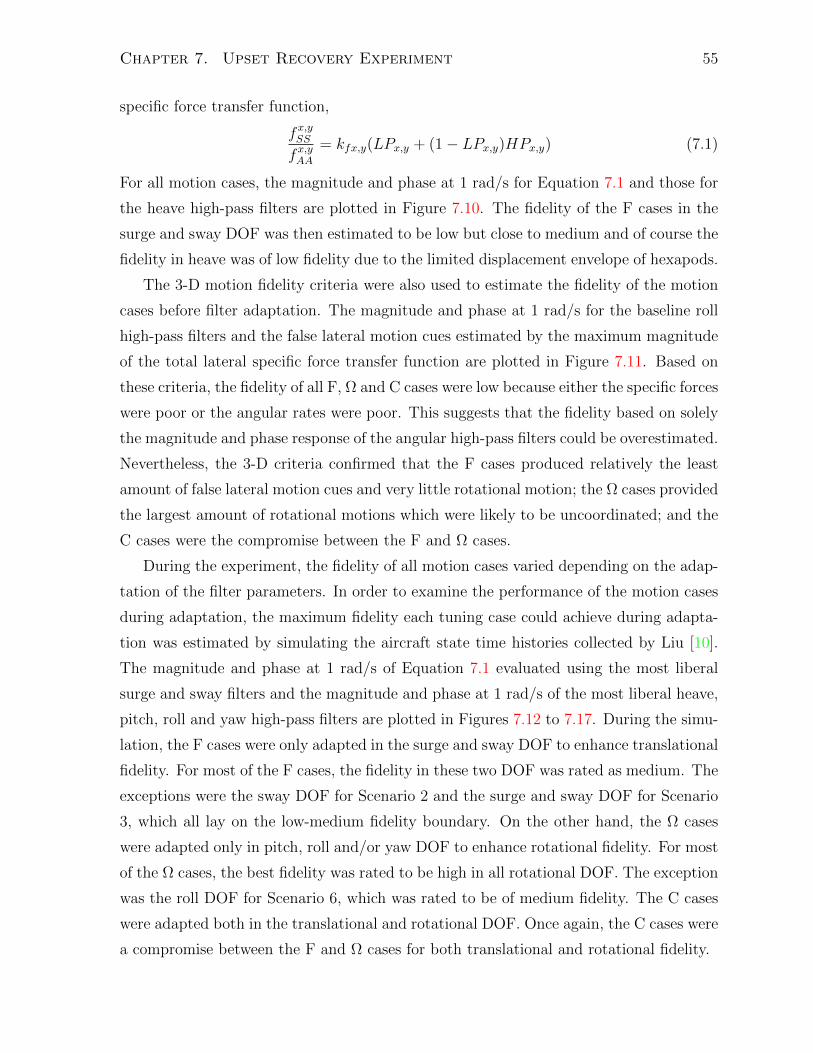
Chapter 7. Upset Recovery Experiment 55
specific force transfer function,
fx,ySS
fx,yAA
= kfx,y(LPx,y + (1− LPx,y)HPx,y) (7.1)
For all motion cases, the magnitude and phase at 1 rad/s for Equation 7.1 and those for
the heave high-pass filters are plotted in Figure 7.10. The fidelity of the F cases in the
surge and sway DOF was then estimated to be low but close to medium and of course the
fidelity in heave was of low fidelity due to the limited displacement envelope of hexapods.
The 3-D motion fidelity criteria were also used to estimate the fidelity of the motion
cases before filter adaptation. The magnitude and phase at 1 rad/s for the baseline roll
high-pass filters and the false lateral motion cues estimated by the maximum magnitude
of the total lateral specific force transfer function are plotted in Figure 7.11. Based on
these criteria, the fidelity of all F, Ω and C cases were low because either the specific forces
were poor or the angular rates were poor. This suggests that the fidelity based on solely
the magnitude and phase response of the angular high-pass filters could be overestimated.
Nevertheless, the 3-D criteria confirmed that the F cases produced relatively the least
amount of false lateral motion cues and very little rotational motion; the Ω cases provided
the largest amount of rotational motions which were likely to be uncoordinated; and the
C cases were the compromise between the F and Ω cases.
During the experiment, the fidelity of all motion cases varied depending on the adap-
tation of the filter parameters. In order to examine the performance of the motion cases
during adaptation, the maximum fidelity each tuning case could achieve during adapta-
tion was estimated by simulating the aircraft state time histories collected by Liu [10].
The magnitude and phase at 1 rad/s of Equation 7.1 evaluated using the most liberal
surge and sway filters and the magnitude and phase at 1 rad/s of the most liberal heave,
pitch, roll and yaw high-pass filters are plotted in Figures 7.12 to 7.17. During the simu-
lation, the F cases were only adapted in the surge and sway DOF to enhance translational
fidelity. For most of the F cases, the fidelity in these two DOF was rated as medium. The
exceptions were the sway DOF for Scenario 2 and the surge and sway DOF for Scenario
3, which all lay on the low-medium fidelity boundary. On the other hand, the Ω cases
were adapted only in pitch, roll and/or yaw DOF to enhance rotational fidelity. For most
of the Ω cases, the best fidelity was rated to be high in all rotational DOF. The exception
was the roll DOF for Scenario 6, which was rated to be of medium fidelity. The C cases
were adapted both in the translational and rotational DOF. Once again, the C cases were
a compromise between the F and Ω cases for both translational and rotational fidelity.
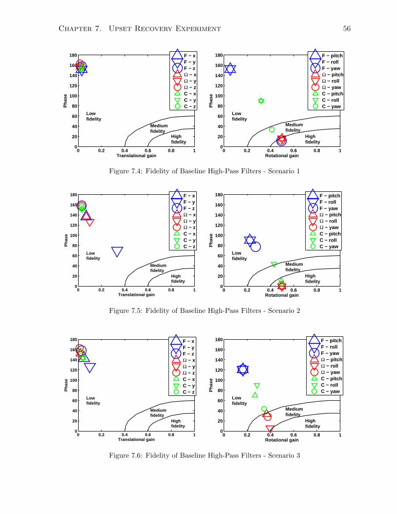
Chapter 7. Upset Recovery Experiment 56
0 0.2 0.4 0.6 0.8 10
20
40
60
80
100
120
140
160
180
Translational gain
Ph
ase
Highfidelity
Mediumfidelity
Lowfidelity
F − xF − yF − zΩ − xΩ − yΩ − zC − xC − yC − z
0 0.2 0.4 0.6 0.8 10
20
40
60
80
100
120
140
160
180
Rotational gain
Ph
ase
Highfidelity
Mediumfidelity
Lowfidelity
F − pitchF − rollF − yawΩ − pitchΩ − rollΩ − yawC − pitchC − rollC − yaw
Figure 7.4: Fidelity of Baseline High-Pass Filters - Scenario 1
0 0.2 0.4 0.6 0.8 10
20
40
60
80
100
120
140
160
180
Translational gain
Ph
ase
Highfidelity
Mediumfidelity
Lowfidelity
F − xF − yF − zΩ − xΩ − yΩ − zC − xC − yC − z
0 0.2 0.4 0.6 0.8 10
20
40
60
80
100
120
140
160
180
Rotational gain
Ph
ase
Highfidelity
Mediumfidelity
Lowfidelity
F − pitchF − rollF − yawΩ − pitchΩ − rollΩ − yawC − pitchC − rollC − yaw
Figure 7.5: Fidelity of Baseline High-Pass Filters - Scenario 2
0 0.2 0.4 0.6 0.8 10
20
40
60
80
100
120
140
160
180
Translational gain
Ph
ase
Highfidelity
Mediumfidelity
Lowfidelity
F − xF − yF − zΩ − xΩ − yΩ − zC − xC − yC − z
0 0.2 0.4 0.6 0.8 10
20
40
60
80
100
120
140
160
180
Rotational gain
Ph
ase
Highfidelity
Mediumfidelity
Lowfidelity
F − pitchF − rollF − yawΩ − pitchΩ − rollΩ − yawC − pitchC − rollC − yaw
Figure 7.6: Fidelity of Baseline High-Pass Filters - Scenario 3
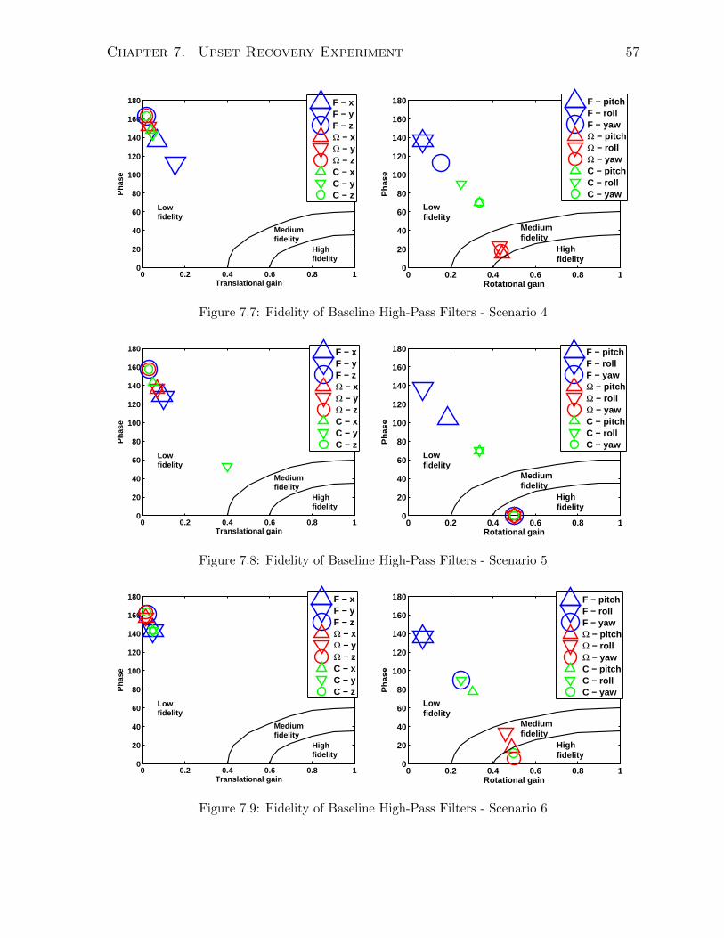
Chapter 7. Upset Recovery Experiment 57
0 0.2 0.4 0.6 0.8 10
20
40
60
80
100
120
140
160
180
Translational gain
Ph
ase
Highfidelity
Mediumfidelity
Lowfidelity
F − xF − yF − zΩ − xΩ − yΩ − zC − xC − yC − z
0 0.2 0.4 0.6 0.8 10
20
40
60
80
100
120
140
160
180
Rotational gain
Ph
ase
Highfidelity
Mediumfidelity
Lowfidelity
F − pitchF − rollF − yawΩ − pitchΩ − rollΩ − yawC − pitchC − rollC − yaw
Figure 7.7: Fidelity of Baseline High-Pass Filters - Scenario 4
0 0.2 0.4 0.6 0.8 10
20
40
60
80
100
120
140
160
180
Translational gain
Ph
ase
Highfidelity
Mediumfidelity
Lowfidelity
F − xF − yF − zΩ − xΩ − yΩ − zC − xC − yC − z
0 0.2 0.4 0.6 0.8 10
20
40
60
80
100
120
140
160
180
Rotational gain
Ph
ase
Highfidelity
Mediumfidelity
Lowfidelity
F − pitchF − rollF − yawΩ − pitchΩ − rollΩ − yawC − pitchC − rollC − yaw
Figure 7.8: Fidelity of Baseline High-Pass Filters - Scenario 5
0 0.2 0.4 0.6 0.8 10
20
40
60
80
100
120
140
160
180
Translational gain
Ph
ase
Highfidelity
Mediumfidelity
Lowfidelity
F − xF − yF − zΩ − xΩ − yΩ − zC − xC − yC − z
0 0.2 0.4 0.6 0.8 10
20
40
60
80
100
120
140
160
180
Rotational gain
Ph
ase
Highfidelity
Mediumfidelity
Lowfidelity
F − pitchF − rollF − yawΩ − pitchΩ − rollΩ − yawC − pitchC − rollC − yaw
Figure 7.9: Fidelity of Baseline High-Pass Filters - Scenario 6
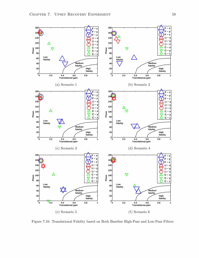
Chapter 7. Upset Recovery Experiment 58
0 0.2 0.4 0.6 0.8 10
20
40
60
80
100
120
140
160
180
Translational gain
Ph
ase
Highfidelity
Mediumfidelity
Lowfidelity
F − xF − yF − zΩ − xΩ − yΩ − zC − xC − yC − z
(a) Scenario 1
0 0.2 0.4 0.6 0.8 10
20
40
60
80
100
120
140
160
180
Translational gain
Ph
ase
Highfidelity
Mediumfidelity
Lowfidelity
F − xF − yF − zΩ − xΩ − yΩ − zC − xC − yC − z
(b) Scenario 2
0 0.2 0.4 0.6 0.8 10
20
40
60
80
100
120
140
160
180
Translational gain
Ph
ase
Highfidelity
Mediumfidelity
Lowfidelity
F − xF − yF − zΩ − xΩ − yΩ − zC − xC − yC − z
(c) Scenario 3
0 0.2 0.4 0.6 0.8 10
20
40
60
80
100
120
140
160
180
Translational gain
Ph
ase
Highfidelity
Mediumfidelity
Lowfidelity
F − xF − yF − zΩ − xΩ − yΩ − zC − xC − yC − z
(d) Scenario 4
0 0.2 0.4 0.6 0.8 10
20
40
60
80
100
120
140
160
180
Translational gain
Ph
ase
Highfidelity
Mediumfidelity
Lowfidelity
F − xF − yF − zΩ − xΩ − yΩ − zC − xC − yC − z
(e) Scenario 5
0 0.2 0.4 0.6 0.8 10
20
40
60
80
100
120
140
160
180
Translational gain
Ph
ase
Highfidelity
Mediumfidelity
Lowfidelity
F − xF − yF − zΩ − xΩ − yΩ − zC − xC − yC − z
(f) Scenario 6
Figure 7.10: Translational Fidelity based on Both Baseline High-Pass and Low-Pass Filters
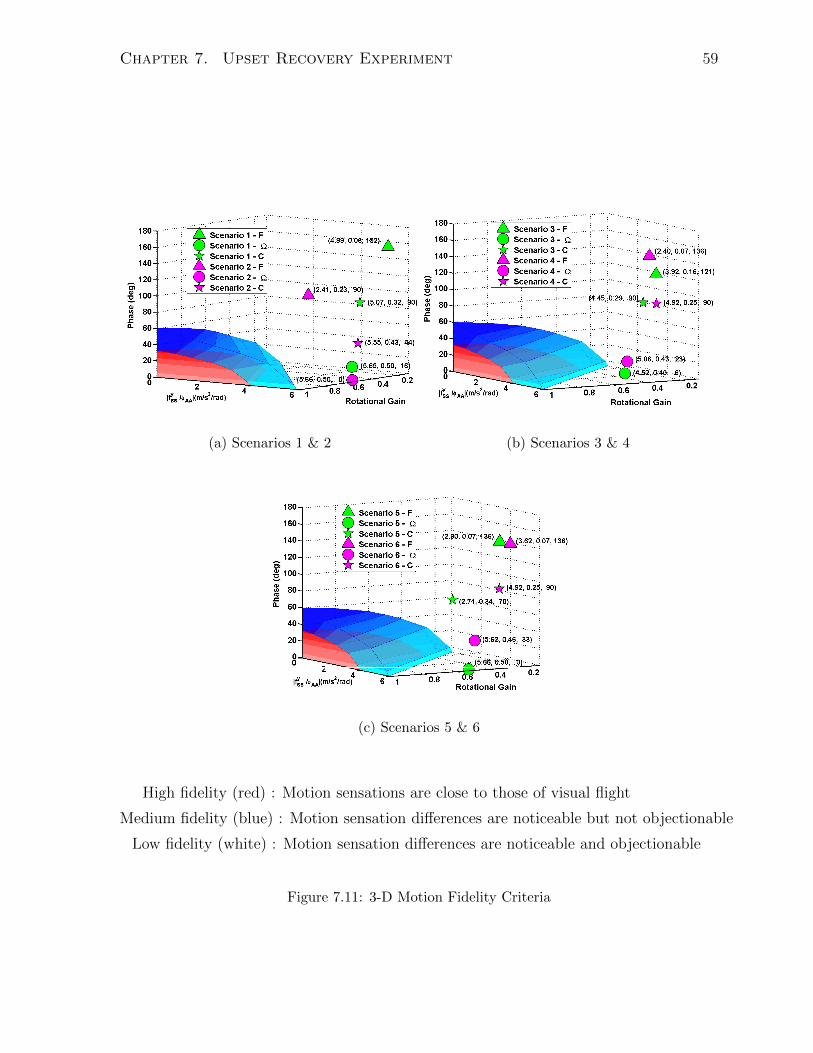
Chapter 7. Upset Recovery Experiment 59
(a) Scenarios 1 & 2 (b) Scenarios 3 & 4
(c) Scenarios 5 & 6
High fidelity (red) : Motion sensations are close to those of visual flight
Medium fidelity (blue) : Motion sensation differences are noticeable but not objectionable
Low fidelity (white) : Motion sensation differences are noticeable and objectionable
Figure 7.11: 3-D Motion Fidelity Criteria
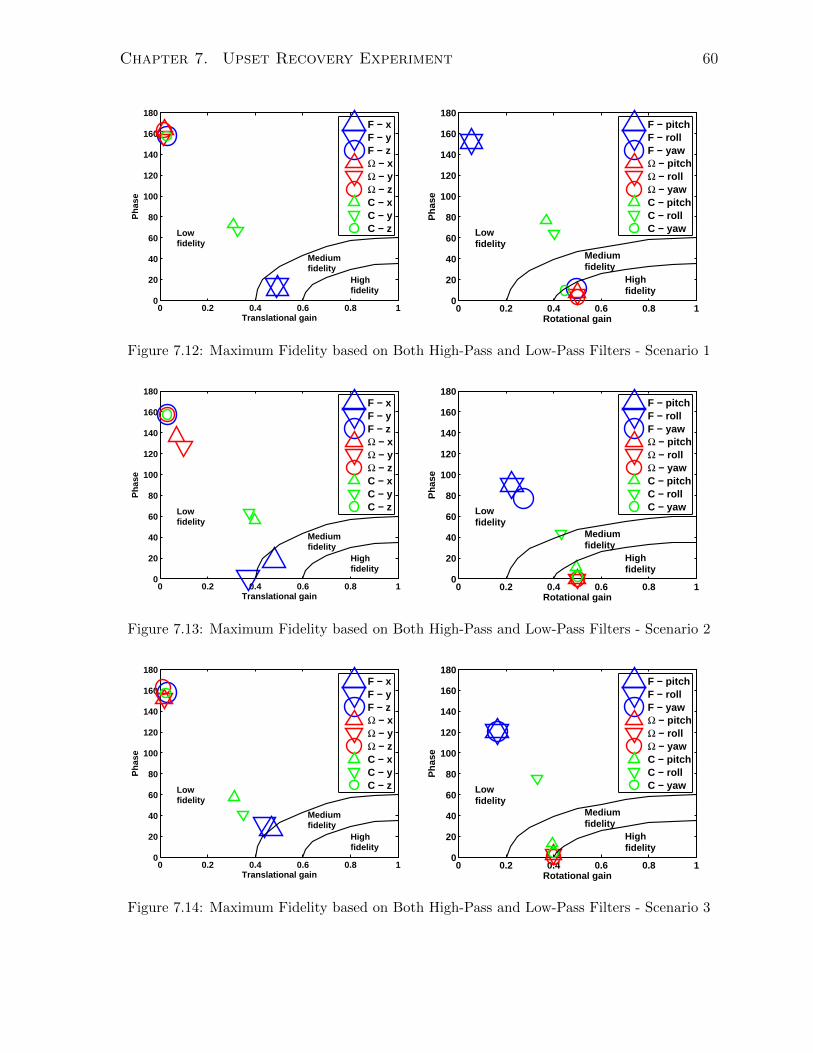
Chapter 7. Upset Recovery Experiment 60
0 0.2 0.4 0.6 0.8 10
20
40
60
80
100
120
140
160
180
Translational gain
Ph
ase
Highfidelity
Mediumfidelity
Lowfidelity
F − xF − yF − zΩ − xΩ − yΩ − zC − xC − yC − z
0 0.2 0.4 0.6 0.8 10
20
40
60
80
100
120
140
160
180
Rotational gain
Ph
ase
Highfidelity
Mediumfidelity
Lowfidelity
F − pitchF − rollF − yawΩ − pitchΩ − rollΩ − yawC − pitchC − rollC − yaw
Figure 7.12: Maximum Fidelity based on Both High-Pass and Low-Pass Filters - Scenario 1
0 0.2 0.4 0.6 0.8 10
20
40
60
80
100
120
140
160
180
Translational gain
Ph
ase
Highfidelity
Mediumfidelity
Lowfidelity
F − xF − yF − zΩ − xΩ − yΩ − zC − xC − yC − z
0 0.2 0.4 0.6 0.8 10
20
40
60
80
100
120
140
160
180
Rotational gain
Ph
ase
Highfidelity
Mediumfidelity
Lowfidelity
F − pitchF − rollF − yawΩ − pitchΩ − rollΩ − yawC − pitchC − rollC − yaw
Figure 7.13: Maximum Fidelity based on Both High-Pass and Low-Pass Filters - Scenario 2
0 0.2 0.4 0.6 0.8 10
20
40
60
80
100
120
140
160
180
Translational gain
Ph
ase
Highfidelity
Mediumfidelity
Lowfidelity
F − xF − yF − zΩ − xΩ − yΩ − zC − xC − yC − z
0 0.2 0.4 0.6 0.8 10
20
40
60
80
100
120
140
160
180
Rotational gain
Ph
ase
Highfidelity
Mediumfidelity
Lowfidelity
F − pitchF − rollF − yawΩ − pitchΩ − rollΩ − yawC − pitchC − rollC − yaw
Figure 7.14: Maximum Fidelity based on Both High-Pass and Low-Pass Filters - Scenario 3
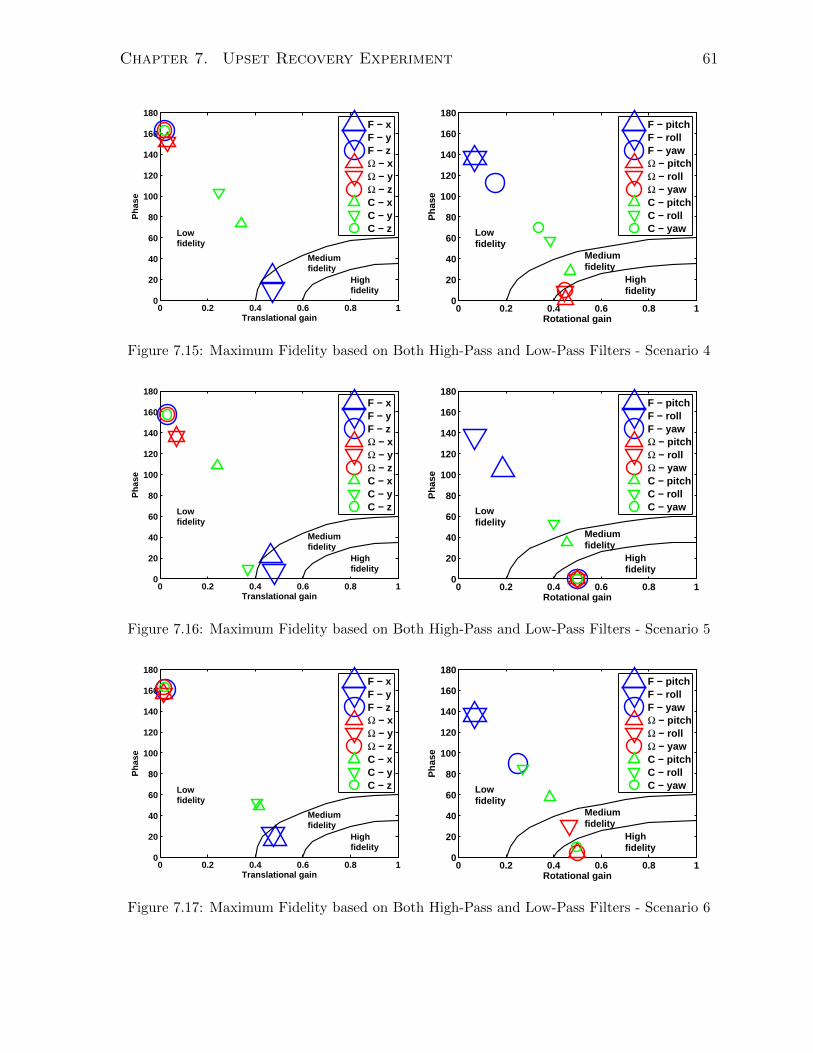
Chapter 7. Upset Recovery Experiment 61
0 0.2 0.4 0.6 0.8 10
20
40
60
80
100
120
140
160
180
Translational gain
Ph
ase
Highfidelity
Mediumfidelity
Lowfidelity
F − xF − yF − zΩ − xΩ − yΩ − zC − xC − yC − z
0 0.2 0.4 0.6 0.8 10
20
40
60
80
100
120
140
160
180
Rotational gain
Ph
ase
Highfidelity
Mediumfidelity
Lowfidelity
F − pitchF − rollF − yawΩ − pitchΩ − rollΩ − yawC − pitchC − rollC − yaw
Figure 7.15: Maximum Fidelity based on Both High-Pass and Low-Pass Filters - Scenario 4
0 0.2 0.4 0.6 0.8 10
20
40
60
80
100
120
140
160
180
Translational gain
Ph
ase
Highfidelity
Mediumfidelity
Lowfidelity
F − xF − yF − zΩ − xΩ − yΩ − zC − xC − yC − z
0 0.2 0.4 0.6 0.8 10
20
40
60
80
100
120
140
160
180
Rotational gain
Ph
ase
Highfidelity
Mediumfidelity
Lowfidelity
F − pitchF − rollF − yawΩ − pitchΩ − rollΩ − yawC − pitchC − rollC − yaw
Figure 7.16: Maximum Fidelity based on Both High-Pass and Low-Pass Filters - Scenario 5
0 0.2 0.4 0.6 0.8 10
20
40
60
80
100
120
140
160
180
Translational gain
Ph
ase
Highfidelity
Mediumfidelity
Lowfidelity
F − xF − yF − zΩ − xΩ − yΩ − zC − xC − yC − z
0 0.2 0.4 0.6 0.8 10
20
40
60
80
100
120
140
160
180
Rotational gain
Ph
ase
Highfidelity
Mediumfidelity
Lowfidelity
F − pitchF − rollF − yawΩ − pitchΩ − rollΩ − yawC − pitchC − rollC − yaw
Figure 7.17: Maximum Fidelity based on Both High-Pass and Low-Pass Filters - Scenario 6
Chapter 7. Upset Recovery Experiment 62
7.1.4 Experimental Procedure
The pilots’ task in this experiment was to fly each of the six upset scenarios for a set of
training trials followed by a set of evaluation trials. The order of the six scenarios assigned
to each pilot was randomized. For each scenario, the training trials were carried out with
no simulator motion except buffet to allow pilots to exercise the recovery techniques
required in the evaluation trials. During the training trials, pilots were required to fly
the scenario repeatedly for 10 minutes until they successfully recovered from it twice. If
no successful recovery was performed within the first 5 minutes, pilots would be supported
with instructions for recovering from the corresponding scenario. For the details of the
recovery techniques for each scenario, see Liu [10].
After pilots successfully recovered from a scenario twice, they proceeded to the evalu-
ation trials of the corresponding scenario. For each scenario, a paired comparison exper-
iment was run during the evaluation trials. Pilots flew the scenario twelve times in six
pairs to compare N to F, N to Ω, N to C, F to Ω, F to C, and Ω to C. The sequence of
these six pairs and the order of the two motion cases in each pair were assigned to pilots
using a randomized ordering. The pairing sequences were different for different scenarios
and the complete list of pairing sequences are shown in Tables C.1 to C.5 in Appendix
C.1. At the end of each paired run, pilots rated the motion fidelity of the motion cases
by choosing one of: (1) the fidelity of the first case was higher than that of the second
case, (2) the fidelity of the second case was higher than that of the first case, or (3) the
two cases were tied in terms of the motion fidelity.
At the end of each flight, the visual displays, excluding the electronic flight instrument
system, were turned off after the simulated aircraft was recovered. Then, the simulator
was brought back to the start-up position. In the meanwhile, pilots were asked to keep
the control column at the steady level flight attitude until the visual display was turned
back on. The purpose of this procedure was to reduce simulator sickness.
The entire experiment session took approximately 4.5 hours, including a 5 to 10
minute break after the completion of every second scenario. Five pilots, including one
flight training instructor and four test pilots, participated in the experiment. All pilots
had previous experience in upset recovery training and aerobatic flying experience. One
pilot had experience flying a B747-200 configuration. Four of the five pilots finished the
entire session in one day, and one pilot finished the session in two different days due to
the stick shaker malfunctioning on the first day.

Chapter 7. Upset Recovery Experiment 63
7.2 Results
The analysis of the experimental results consists of two parts: (1) an analysis of the
subjective paired comparison data, and (2) an analysis of the objective pilot performance
data.
7.2.1 Subjective Paired Comparison Analysis
7.2.1.1 Non-parametric Analysis
The following non-parametric analysis for paired comparison experiments is based on
Butler [41] and it was developed by extending the non-parametric analysis given by
David [42] to allow ties and order effect. The probability that motion condition i is
preferred over motion condition j is given by the pair probability, πij, which is estimated
using
πij = αij/n (7.2)
where n is the total number of times conditions i and j are compared and αij is the total
number of times condition i is selected over j plus half the number of times conditions
i and j are tied. For this experiment, each pair of conditions was tested once by each
pilot, so n = 5 (5 subjects × 1 order). The total score for each motion condition is then,
ai =tc∑j=1
αij (7.3)
where tc is the number of conditions being compared, which is 4, and αii is 0 by definition.
The total scores for the four motion cases for all six scenarios are shown in Table 7.1 and
in Figure 7.18.
The first step in this analysis is to test the null hypothesis, H0, that all measured
scores are statistically equal (i.e. all motion conditions are equally preferred). According
to Butler [41], the expected values of all the scores is n/2× (tc− 1), which is 7.5 for this
experiment, and the variance of all the scores when all motion cases are equally preferred
is given by
σ2ai
=n(tc − 1)
2
[P1(1− P1) + P2(1− P2)− Po(1− Po)
2
](7.4)
The following probabilities are defined under H0,
P1, the probability of selecting the first condition when the conditions are the same
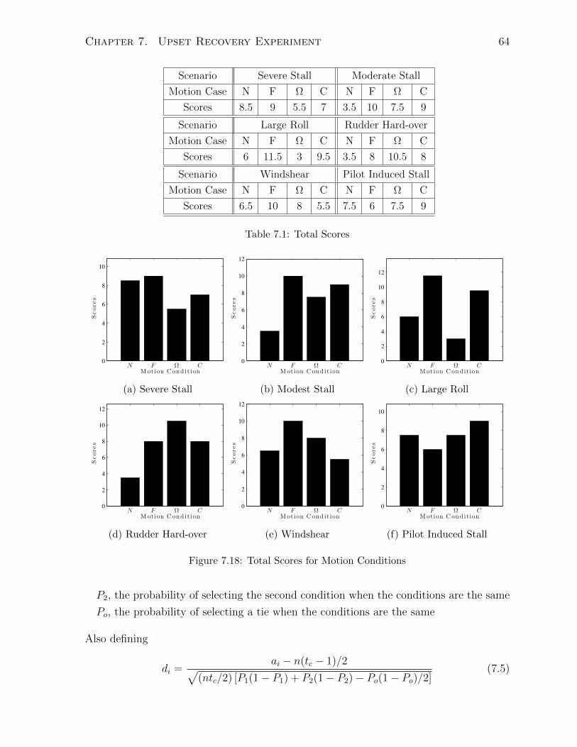
Chapter 7. Upset Recovery Experiment 64
Scenario Severe Stall Moderate Stall
Motion Case N F Ω C N F Ω C
Scores 8.5 9 5.5 7 3.5 10 7.5 9
Scenario Large Roll Rudder Hard-over
Motion Case N F Ω C N F Ω C
Scores 6 11.5 3 9.5 3.5 8 10.5 8
Scenario Windshear Pilot Induced Stall
Motion Case N F Ω C N F Ω C
Scores 6.5 10 8 5.5 7.5 6 7.5 9
Table 7.1: Total Scores
0
2
4
6
8
10
Motion C ond it ion
Score
s
N F Ω C
(a) Severe Stall
0
2
4
6
8
10
12
Motion C ond it ion
Score
s
N F Ω C
(b) Modest Stall
0
2
4
6
8
10
12
Motion C ond it ionScore
sN F Ω C
(c) Large Roll
0
2
4
6
8
10
12
Motion C ond it ion
Score
s
N F Ω C
(d) Rudder Hard-over
0
2
4
6
8
10
12
Motion C ond it ion
Score
s
N F Ω C
(e) Windshear
0
2
4
6
8
10
Motion C ond it ion
Score
s
N F Ω C
(f) Pilot Induced Stall
Figure 7.18: Total Scores for Motion Conditions
P2, the probability of selecting the second condition when the conditions are the same
Po, the probability of selecting a tie when the conditions are the same
Also defining
di =ai − n(tc − 1)/2√
(ntc/2) [P1(1− P1) + P2(1− P2)− Po(1− Po)/2](7.5)
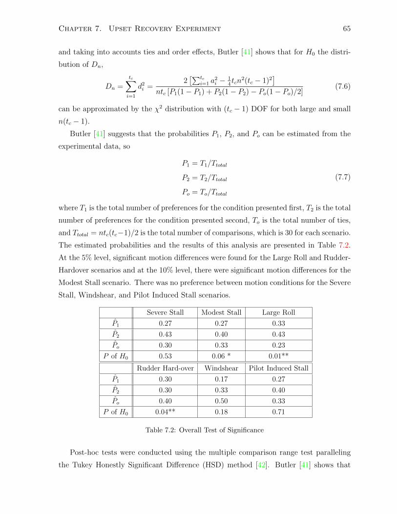
Chapter 7. Upset Recovery Experiment 65
and taking into accounts ties and order effects, Butler [41] shows that for H0 the distri-
bution of Dn,
Dn =tc∑i=1
d2i =
2[∑tc
i=1 a2i − 1
4tcn
2(tc − 1)2]
ntc [P1(1− P1) + P2(1− P2)− Po(1− Po)/2](7.6)
can be approximated by the χ2 distribution with (tc − 1) DOF for both large and small
n(tc − 1).
Butler [41] suggests that the probabilities P1, P2, and Po can be estimated from the
experimental data, so
P1 = T1/Ttotal
P2 = T2/Ttotal
Po = To/Ttotal
(7.7)
where T1 is the total number of preferences for the condition presented first, T2 is the total
number of preferences for the condition presented second, To is the total number of ties,
and Ttotal = ntc(tc−1)/2 is the total number of comparisons, which is 30 for each scenario.
The estimated probabilities and the results of this analysis are presented in Table 7.2.
At the 5% level, significant motion differences were found for the Large Roll and Rudder-
Hardover scenarios and at the 10% level, there were significant motion differences for the
Modest Stall scenario. There was no preference between motion conditions for the Severe
Stall, Windshear, and Pilot Induced Stall scenarios.
Severe Stall Modest Stall Large Roll
P1 0.27 0.27 0.33
P2 0.43 0.40 0.43
Po 0.30 0.33 0.23
P of H0 0.53 0.06 * 0.01**
Rudder Hard-over Windshear Pilot Induced Stall
P1 0.30 0.17 0.27
P2 0.30 0.33 0.40
Po 0.40 0.50 0.33
P of H0 0.04** 0.18 0.71
Table 7.2: Overall Test of Significance
Post-hoc tests were conducted using the multiple comparison range test paralleling
the Tukey Honestly Significant Difference (HSD) method [42]. Butler [41] shows that
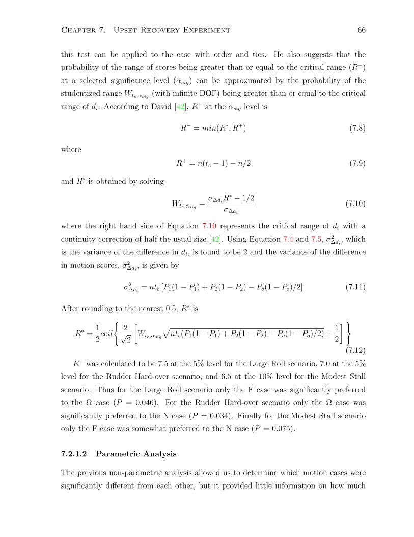
Chapter 7. Upset Recovery Experiment 66
this test can be applied to the case with order and ties. He also suggests that the
probability of the range of scores being greater than or equal to the critical range (R−)
at a selected significance level (αsig) can be approximated by the probability of the
studentized range Wtc,αsig (with infinite DOF) being greater than or equal to the critical
range of di. According to David [42], R− at the αsig level is
R− = min(R∗, R+) (7.8)
where
R+ = n(tc − 1)− n/2 (7.9)
and R∗ is obtained by solving
Wtc,αsig =σ∆diR
∗ − 1/2
σ∆ai
(7.10)
where the right hand side of Equation 7.10 represents the critical range of di with a
continuity correction of half the usual size [42]. Using Equation 7.4 and 7.5, σ2∆di
, which
is the variance of the difference in di, is found to be 2 and the variance of the difference
in motion scores, σ2∆ai
, is given by
σ2∆ai
= ntc [P1(1− P1) + P2(1− P2)− Po(1− Po)/2] (7.11)
After rounding to the nearest 0.5, R∗ is
R∗ =1
2ceil
2√2
[Wtc,αsig
√ntc(P1(1− P1) + P2(1− P2)− Po(1− Po)/2) +
1
2
](7.12)
R− was calculated to be 7.5 at the 5% level for the Large Roll scenario, 7.0 at the 5%
level for the Rudder Hard-over scenario, and 6.5 at the 10% level for the Modest Stall
scenario. Thus for the Large Roll scenario only the F case was significantly preferred
to the Ω case (P = 0.046). For the Rudder Hard-over scenario only the Ω case was
significantly preferred to the N case (P = 0.034). Finally for the Modest Stall scenario
only the F case was somewhat preferred to the N case (P = 0.075).
7.2.1.2 Parametric Analysis
The previous non-parametric analysis allowed us to determine which motion cases were
significantly different from each other, but it provided little information on how much
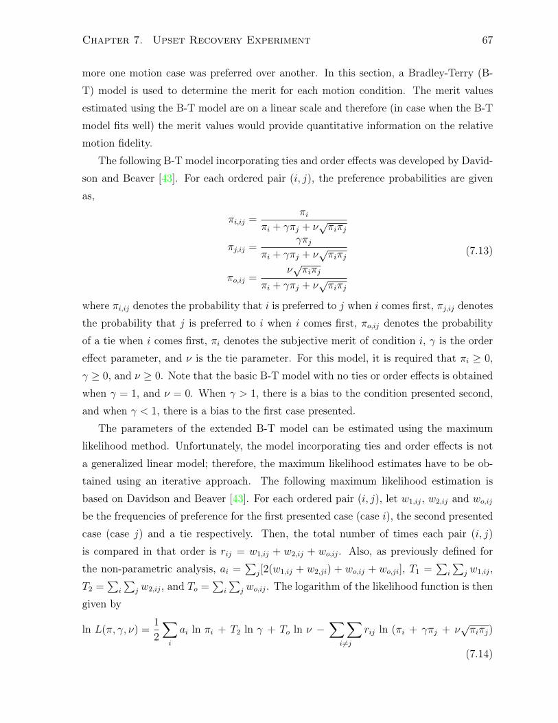
Chapter 7. Upset Recovery Experiment 67
more one motion case was preferred over another. In this section, a Bradley-Terry (B-
T) model is used to determine the merit for each motion condition. The merit values
estimated using the B-T model are on a linear scale and therefore (in case when the B-T
model fits well) the merit values would provide quantitative information on the relative
motion fidelity.
The following B-T model incorporating ties and order effects was developed by David-
son and Beaver [43]. For each ordered pair (i, j), the preference probabilities are given
as,
πi,ij =πi
πi + γπj + ν√πiπj
πj,ij =γπj
πi + γπj + ν√πiπj
πo,ij =ν√πiπj
πi + γπj + ν√πiπj
(7.13)
where πi,ij denotes the probability that i is preferred to j when i comes first, πj,ij denotes
the probability that j is preferred to i when i comes first, πo,ij denotes the probability
of a tie when i comes first, πi denotes the subjective merit of condition i, γ is the order
effect parameter, and ν is the tie parameter. For this model, it is required that πi ≥ 0,
γ ≥ 0, and ν ≥ 0. Note that the basic B-T model with no ties or order effects is obtained
when γ = 1, and ν = 0. When γ > 1, there is a bias to the condition presented second,
and when γ < 1, there is a bias to the first case presented.
The parameters of the extended B-T model can be estimated using the maximum
likelihood method. Unfortunately, the model incorporating ties and order effects is not
a generalized linear model; therefore, the maximum likelihood estimates have to be ob-
tained using an iterative approach. The following maximum likelihood estimation is
based on Davidson and Beaver [43]. For each ordered pair (i, j), let w1,ij, w2,ij and wo,ij
be the frequencies of preference for the first presented case (case i), the second presented
case (case j) and a tie respectively. Then, the total number of times each pair (i, j)
is compared in that order is rij = w1,ij + w2,ij + wo,ij. Also, as previously defined for
the non-parametric analysis, ai =∑
j[2(w1,ij + w2,ji) + wo,ij + wo,ji], T1 =∑
i
∑j w1,ij,
T2 =∑
i
∑j w2,ij, and To =
∑i
∑j wo,ij. The logarithm of the likelihood function is then
given by
ln L(π, γ, ν) =1
2
∑i
ai ln πi + T2 ln γ + To ln ν −∑∑
i 6=j
rij ln (πi + γπj + ν√πiπj)
(7.14)
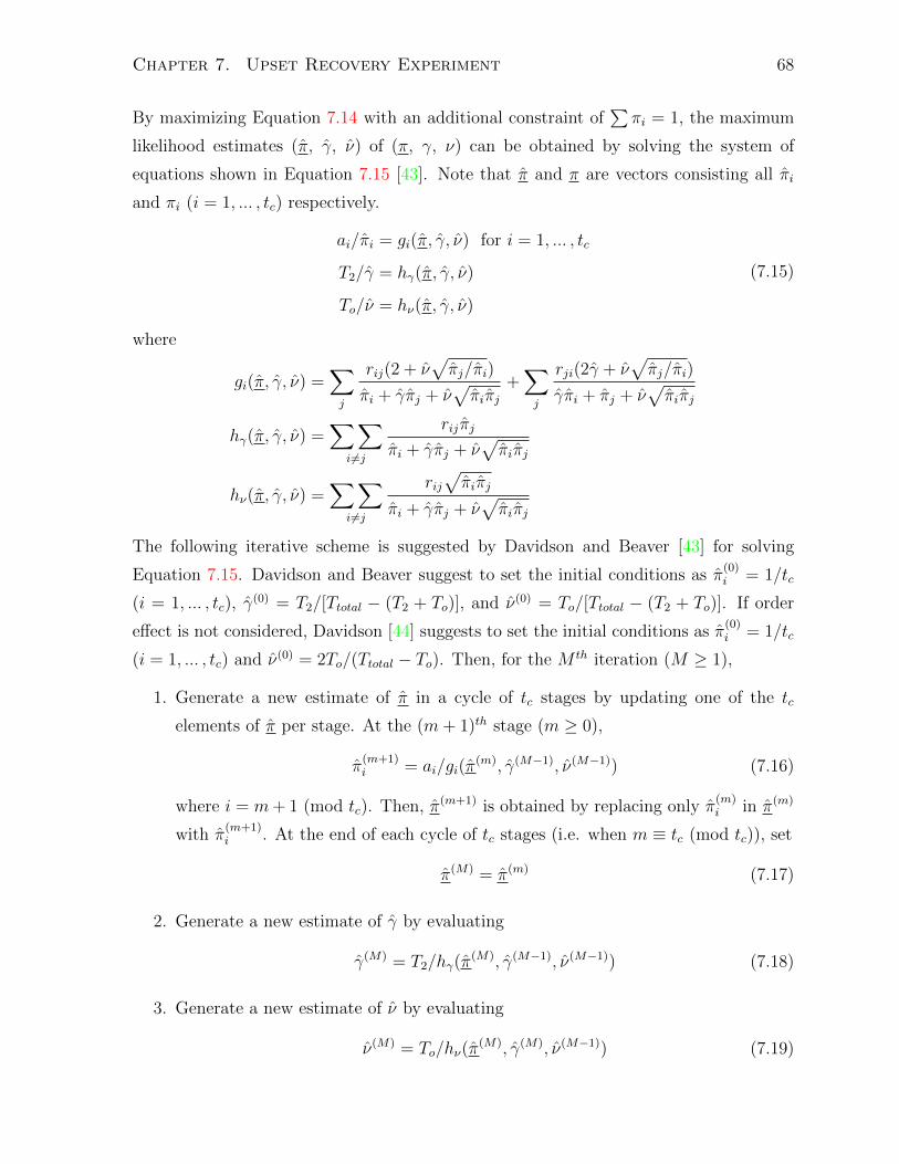
Chapter 7. Upset Recovery Experiment 68
By maximizing Equation 7.14 with an additional constraint of∑πi = 1, the maximum
likelihood estimates (π, γ, ν) of (π, γ, ν) can be obtained by solving the system of
equations shown in Equation 7.15 [43]. Note that π and π are vectors consisting all πi
and πi (i = 1, ... , tc) respectively.
ai/πi = gi(π, γ, ν) for i = 1, ... , tc
T2/γ = hγ(π, γ, ν)
To/ν = hν(π, γ, ν)
(7.15)
where
gi(π, γ, ν) =∑j
rij(2 + ν√πj/πi)
πi + γπj + ν√πiπj
+∑j
rji(2γ + ν√πj/πi)
γπi + πj + ν√πiπj
hγ(π, γ, ν) =∑∑
i 6=j
rijπj
πi + γπj + ν√πiπj
hν(π, γ, ν) =∑∑
i 6=j
rij√πiπj
πi + γπj + ν√πiπj
The following iterative scheme is suggested by Davidson and Beaver [43] for solving
Equation 7.15. Davidson and Beaver suggest to set the initial conditions as π(0)i = 1/tc
(i = 1, ... , tc), γ(0) = T2/[Ttotal − (T2 + To)], and ν(0) = To/[Ttotal − (T2 + To)]. If order
effect is not considered, Davidson [44] suggests to set the initial conditions as π(0)i = 1/tc
(i = 1, ... , tc) and ν(0) = 2To/(Ttotal − To). Then, for the M th iteration (M ≥ 1),
1. Generate a new estimate of π in a cycle of tc stages by updating one of the tc
elements of π per stage. At the (m+ 1)th stage (m ≥ 0),
π(m+1)i = ai/gi(π
(m), γ(M−1), ν(M−1)) (7.16)
where i = m+ 1 (mod tc). Then, π(m+1) is obtained by replacing only π(m)i in π(m)
with π(m+1)i . At the end of each cycle of tc stages (i.e. when m ≡ tc (mod tc)), set
π(M) = π(m) (7.17)
2. Generate a new estimate of γ by evaluating
γ(M) = T2/hγ(π(M), γ(M−1), ν(M−1)) (7.18)
3. Generate a new estimate of ν by evaluating
ν(M) = To/hν(π(M), γ(M), ν(M−1)) (7.19)
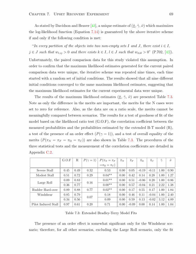
Chapter 7. Upset Recovery Experiment 69
As stated by Davidson and Beaver [43], a unique estimate of (π, γ, ν) which maximizes
the log-likelihood function (Equation 7.14) is guaranteed by the above iterative scheme
if and only if the following condition is met:
“In every partition of the objects into two non-empty sets I and J , there exist i ∈ I,
j ∈ J such that w1,ij > 0 and there exists k ∈ I, l ∈ J such that w2,kl > 0” (P.702, [43]).
Unfortunately, the paired comparison data for this study violated this assumption. In
order to confirm that the maximum likelihood estimates generated for the current paired
comparison data were unique, the iterative scheme was repeated nine times, each time
started with a random set of initial conditions. The results showed that all nine different
initial conditions converged to the same maximum likelihood estimates, suggesting that
the maximum likelihood estimates for the current experimental data were unique.
The results of the maximum likelihood estimates (π, γ, ν) are presented Table 7.3.
Note as only the difference in the merits are important, the merits for the N cases were
set to zero for reference. Also, as the data are on a ratio scale, the merits cannot be
meaningfully compared between scenarios. The results for a test of goodness of fit of the
model based on the likelihood ratio test (G.O.F), the correlation coefficient between the
measured probabilities and the probabilities estimated by the extended B-T model (R),
a test of the presence of an order effect (P (γ = 1)), and a test of overall equality of the
merits (P (πN = πF = πΩ = πC)) are also shown in Table 7.3. The procedures of the
three statistical tests and the measurement of the correlation coefficients are detailed in
Appendix C.2.
G.O.F R P (γ = 1) P (πN = πF πN πF πΩ πC γ ν
=πΩ = πC)
Severe Stall 0.45 0.49 0.32 0.53 0.00 0.05 -0.19 -0.11 1.00 0.90
Modest Stall 0.51 0.72 0.29 0.04** 0.00 0.42 0.14 0.28 1.00 1.27
Large Roll0.09 0.83
0.160.01** 0.00 0.51 -0.06 0.20 1.00 0.86
0.36 0.77 0.00** 0.00 0.57 -0.04 0.21 2.22 1.38
Rudder Hard-over 0.89 0.88 0.77 0.02** 0.00 0.17 0.55 0.17 1.00 1.84
Windshear 0.85 0.790.07
0.18 0.00 0.46 0.11 -0.04 1.00 2.40
0.34 0.56 0.09 0.00 0.59 0.13 -0.02 3.12 4.89
Pilot Induced Stall 0.97 0.61 0.20 0.71 0.00 -0.09 0.00 0.14 1.00 1.04
Table 7.3: Extended Bradley-Terry Model Fits
The presence of an order effect is somewhat significant only for the Windshear sce-
nario; therefore, for all other scenarios, excluding the Large Roll scenario, only the fit
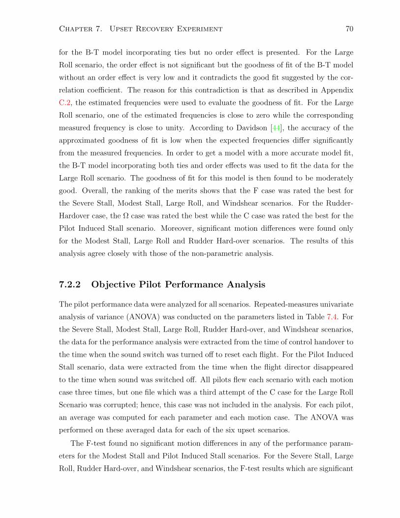
Chapter 7. Upset Recovery Experiment 70
for the B-T model incorporating ties but no order effect is presented. For the Large
Roll scenario, the order effect is not significant but the goodness of fit of the B-T model
without an order effect is very low and it contradicts the good fit suggested by the cor-
relation coefficient. The reason for this contradiction is that as described in Appendix
C.2, the estimated frequencies were used to evaluate the goodness of fit. For the Large
Roll scenario, one of the estimated frequencies is close to zero while the corresponding
measured frequency is close to unity. According to Davidson [44], the accuracy of the
approximated goodness of fit is low when the expected frequencies differ significantly
from the measured frequencies. In order to get a model with a more accurate model fit,
the B-T model incorporating both ties and order effects was used to fit the data for the
Large Roll scenario. The goodness of fit for this model is then found to be moderately
good. Overall, the ranking of the merits shows that the F case was rated the best for
the Severe Stall, Modest Stall, Large Roll, and Windshear scenarios. For the Rudder-
Hardover case, the Ω case was rated the best while the C case was rated the best for the
Pilot Induced Stall scenario. Moreover, significant motion differences were found only
for the Modest Stall, Large Roll and Rudder Hard-over scenarios. The results of this
analysis agree closely with those of the non-parametric analysis.
7.2.2 Objective Pilot Performance Analysis
The pilot performance data were analyzed for all scenarios. Repeated-measures univariate
analysis of variance (ANOVA) was conducted on the parameters listed in Table 7.4. For
the Severe Stall, Modest Stall, Large Roll, Rudder Hard-over, and Windshear scenarios,
the data for the performance analysis were extracted from the time of control handover to
the time when the sound switch was turned off to reset each flight. For the Pilot Induced
Stall scenario, data were extracted from the time when the flight director disappeared
to the time when sound was switched off. All pilots flew each scenario with each motion
case three times, but one file which was a third attempt of the C case for the Large Roll
Scenario was corrupted; hence, this case was not included in the analysis. For each pilot,
an average was computed for each parameter and each motion case. The ANOVA was
performed on these averaged data for each of the six upset scenarios.
The F-test found no significant motion differences in any of the performance param-
eters for the Modest Stall and Pilot Induced Stall scenarios. For the Severe Stall, Large
Roll, Rudder Hard-over, and Windshear scenarios, the F-test results which are significant
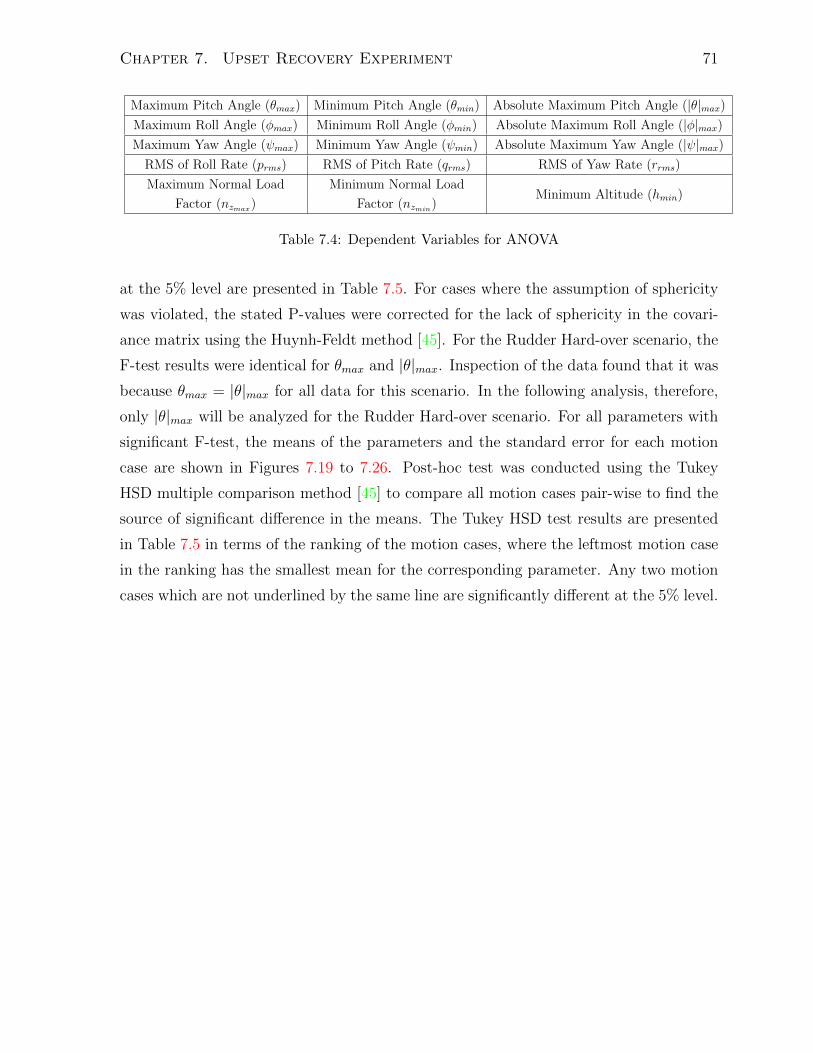
Chapter 7. Upset Recovery Experiment 71
Maximum Pitch Angle (θmax) Minimum Pitch Angle (θmin) Absolute Maximum Pitch Angle (|θ|max)Maximum Roll Angle (φmax) Minimum Roll Angle (φmin) Absolute Maximum Roll Angle (|φ|max)Maximum Yaw Angle (ψmax) Minimum Yaw Angle (ψmin) Absolute Maximum Yaw Angle (|ψ|max)
RMS of Roll Rate (prms) RMS of Pitch Rate (qrms) RMS of Yaw Rate (rrms)
Maximum Normal Load Minimum Normal LoadMinimum Altitude (hmin)
Factor (nzmax) Factor (nzmin)
Table 7.4: Dependent Variables for ANOVA
at the 5% level are presented in Table 7.5. For cases where the assumption of sphericity
was violated, the stated P-values were corrected for the lack of sphericity in the covari-
ance matrix using the Huynh-Feldt method [45]. For the Rudder Hard-over scenario, the
F-test results were identical for θmax and |θ|max. Inspection of the data found that it was
because θmax = |θ|max for all data for this scenario. In the following analysis, therefore,
only |θ|max will be analyzed for the Rudder Hard-over scenario. For all parameters with
significant F-test, the means of the parameters and the standard error for each motion
case are shown in Figures 7.19 to 7.26. Post-hoc test was conducted using the Tukey
HSD multiple comparison method [45] to compare all motion cases pair-wise to find the
source of significant difference in the means. The Tukey HSD test results are presented
in Table 7.5 in terms of the ranking of the motion cases, where the leftmost motion case
in the ranking has the smallest mean for the corresponding parameter. Any two motion
cases which are not underlined by the same line are significantly different at the 5% level.
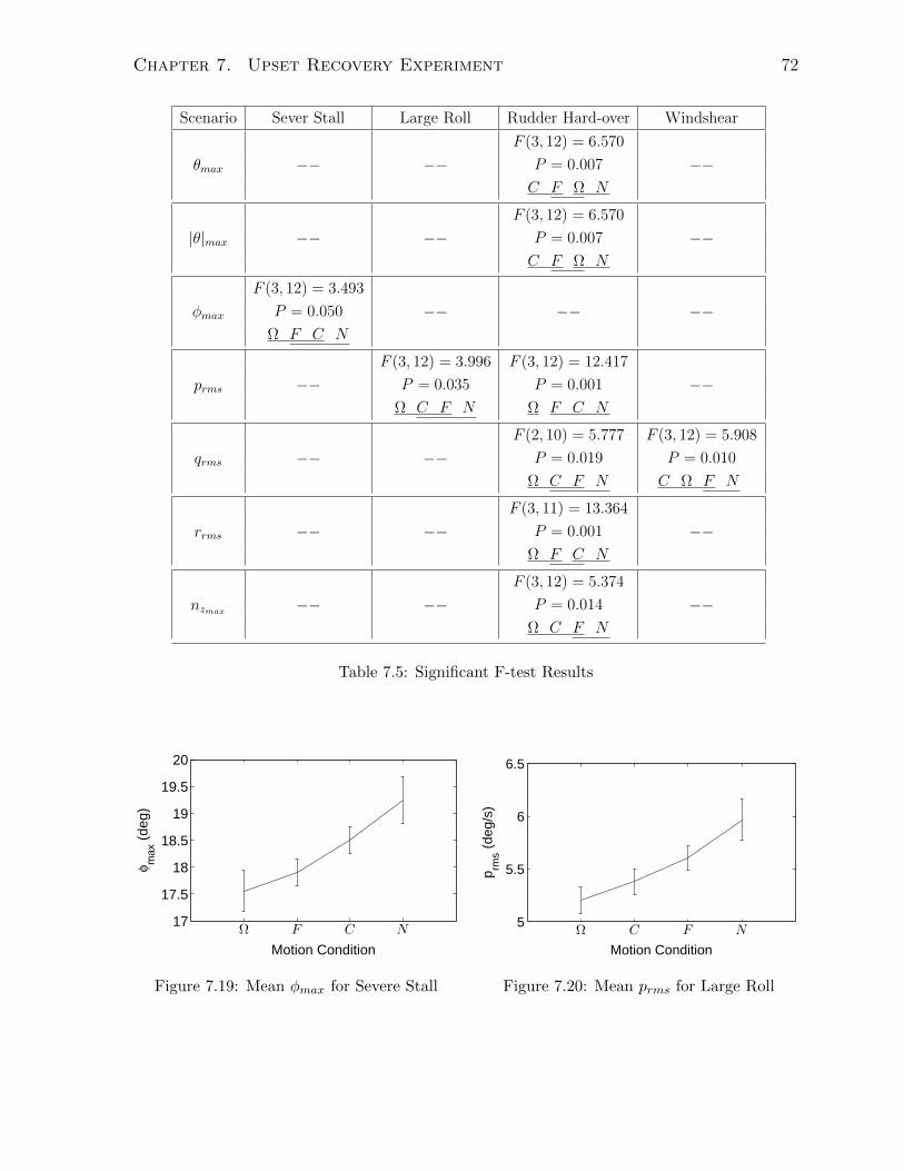
Chapter 7. Upset Recovery Experiment 72
Scenario Sever Stall Large Roll Rudder Hard-over Windshear
θmax −− −−F (3, 12) = 6.570
−−P = 0.007
C F Ω N
|θ|max −− −−F (3, 12) = 6.570
−−P = 0.007
C F Ω N
φmax
F (3, 12) = 3.493
−− −− −−P = 0.050
Ω F C N
prms −−F (3, 12) = 3.996 F (3, 12) = 12.417
−−P = 0.035 P = 0.001
Ω C F N Ω F C N
qrms −− −−F (2, 10) = 5.777 F (3, 12) = 5.908
P = 0.019 P = 0.010
Ω C F N C Ω F N
rrms −− −−F (3, 11) = 13.364
−−P = 0.001
Ω F C N
nzmax −− −−F (3, 12) = 5.374
−−P = 0.014
Ω C F N
Table 7.5: Significant F-test Results
17
17.5
18
18.5
19
19.5
20
Ω F C N
Motion Condition
φ max
(de
g)
Figure 7.19: Mean φmax for Severe Stall
5
5.5
6
6.5
Ω C F N
Motion Condition
p rms (
deg/
s)
Figure 7.20: Mean prms for Large Roll
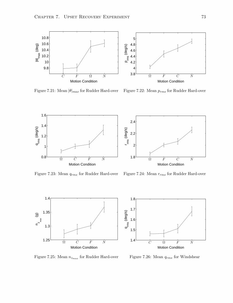
Chapter 7. Upset Recovery Experiment 73
9.8
10
10.2
10.4
10.6
10.8
C F Ω N
Motion Condition
|θ| m
ax (
deg)
Figure 7.21: Mean |θ|max for Rudder Hard-over
3.8
4
4.2
4.4
4.6
4.8
5
Ω F C N
Motion Condition
p rms (
deg/
s)
Figure 7.22: Mean prms for Rudder Hard-over
0.8
1
1.2
1.4
1.6
Ω C F N
Motion Condition
q rms (
deg/
s)
Figure 7.23: Mean qrms for Rudder Hard-over
1.8
2
2.2
2.4
Ω F C N
Motion Condition
r rms (
deg/
s)
Figure 7.24: Mean rrms for Rudder Hard-over
1.25
1.3
1.35
1.4
Ω C F N
Motion Condition
n z max
(g)
Figure 7.25: Mean nzmax for Rudder Hard-over
1.4
1.5
1.6
1.7
1.8
C Ω F N
Motion Condition
q rms (
deg/
s)
Figure 7.26: Mean qrms for Windshear
Chapter 7. Upset Recovery Experiment 74
7.3 Discussion of Results
For the Large Roll scenario, there was a strong preference for the F motion case and a
strong dislike for the Ω motion case with the compromise C being somewhat preferred
to the N case. The most likely explanation for this preference is the large lateral specific
force errors that occurred when an attempt was made to simulate the large roll motion.
In fact, three of the five pilots commented on the uncoordinated roll maneuvers and
mentioned that they did not prefer the strong side force in the Ω case of this scenario.
For other than the N case, the subjective fidelity ranking was identical to that given by
the minimization of the lateral specific force false cues. N was rated inferior to both F and
C likely because the false cues for these cases were not too large yet they still produced
motion. On the other hand, the performance analysis found that the root mean square
of the roll rate was significantly smaller for the Ω case than the N case. According to this
analysis, the value of prms was in fact inversely proportional to the fidelity of roll cues in
each motion case. As no significant differences were detected in the roll angle, a smaller
value of prms would mean that the aircraft was recovered using less aggressive dynamic
roll motions without causing the roll attitude to diverge, indicating better lateral control.
Hence, if prms is considered a representative measure of lateral control, the fidelity of roll
cues is then directly related to the degree of lateral control in the Large Roll scenario.
Also, the contradiction between the two analysis suggests that the specific force false
cues associated with the roll motion cues may in effect be subjectively cancelling out the
benefits of the improved lateral control.
For the Rudder Hard-over scenario, the Ω case was most preferred and the N case
was the least preferred. The other two cases were the same and fell between these two
extremes. This seems like a curious result given our previous explanation of lateral specific
force false cues. In fact, no pilots commented on the amount of lateral specific force false
cues during the testing of the Rudder Hard-over scenario. One possible explanation for
this is that the roll attitude for the Rudder Hard-over event was generally smaller than
that for the Large Roll scenario, so the roll cues could be generated for good lateral
motion cueing without the associated large false lateral cues. The benefit of the roll cues
was confirmed by the performance analysis. prms was found be to significantly smaller in
the Ω case than in any other motion cases for this scenario while no significant differences
were detected in the roll angle. Moreover, rrms was also found to be significantly smaller
for the Ω than the C and N cases with no significant differences found in the yaw angle.
Chapter 7. Upset Recovery Experiment 75
This suggests that the presence of roll cues and yaw cues helped improve the lateral and
directional control in the event of rudder hard-over. The performance analysis also found
that the maximum normal load factor was significantly higher for the N case than any
other motion cases, suggesting that pilots tended to pull harder on the column in order to
roll aircraft back towards the wings-level flight when no motion cues were present. Lastly,
qrms was smaller for the Ω case than for the C and F cases while it was significantly smaller
than for the N case. In contrary, |θ|max was significantly smaller for the C case than both
the Ω and N cases. This suggests that high fidelity pitch motion does not necessarily lead
to improvements for the longitudinal control, but a compromise between specific force
cues and angular cues may lead to a good balance between the aircraft dynamic pitch
motion and pitch attitude for recovering a rudder hard-over scenario.
There was little preference for any of the motion conditions for the Windshear sce-
nario. In particular, the fit of the extended B-T model for this scenario determined a
high value for the tie parameter (ν = 4.89) and a probability of the presence of order
effect that was close to being significant at the 5% level. This suggests that pilots tended
to choose a tie or the motion case that was presented last in each pair. In fact, three
pilots found that the motions for this scenario were generally too subtle in all motion
cases. The performance analysis found that the root mean square values of the pitch rate
of both the C and Ω cases were significantly smaller than that of the N case. Although
no consensus was achieved between the subjective fidelity analysis and the performance
analysis, the results of this performance analysis agree with those of the Rudder Hard-
over scenario that a compromise between translational and rotational cues may lead to
better longitudinal control.
For the Severe Stall scenario, analysis of the performance data found that the max-
imum roll angle was significantly smaller for the Ω case than for the N case, but there
were no significant motion differences in terms of the minimum roll angle or the absolute
maximum roll angle. Generally, the maximum roll angle gives an indication of the pilot
performance for maintaining lateral control when the aircraft rolls to the right (with
smaller values indicating better control), and for this experiment, right was set as the
direction for the asymmetric stall roll-off. If the maximum roll angle is considered to be
a representative measure of lateral control, then it seems that the fidelity of roll cues was
closely related the degree of control for the aircraft’s initial divergent lateral-directional
responses. In order to confirm this claim, the data for the first maximum roll angle
that occurred after control handover (between control handover and about 10 seconds
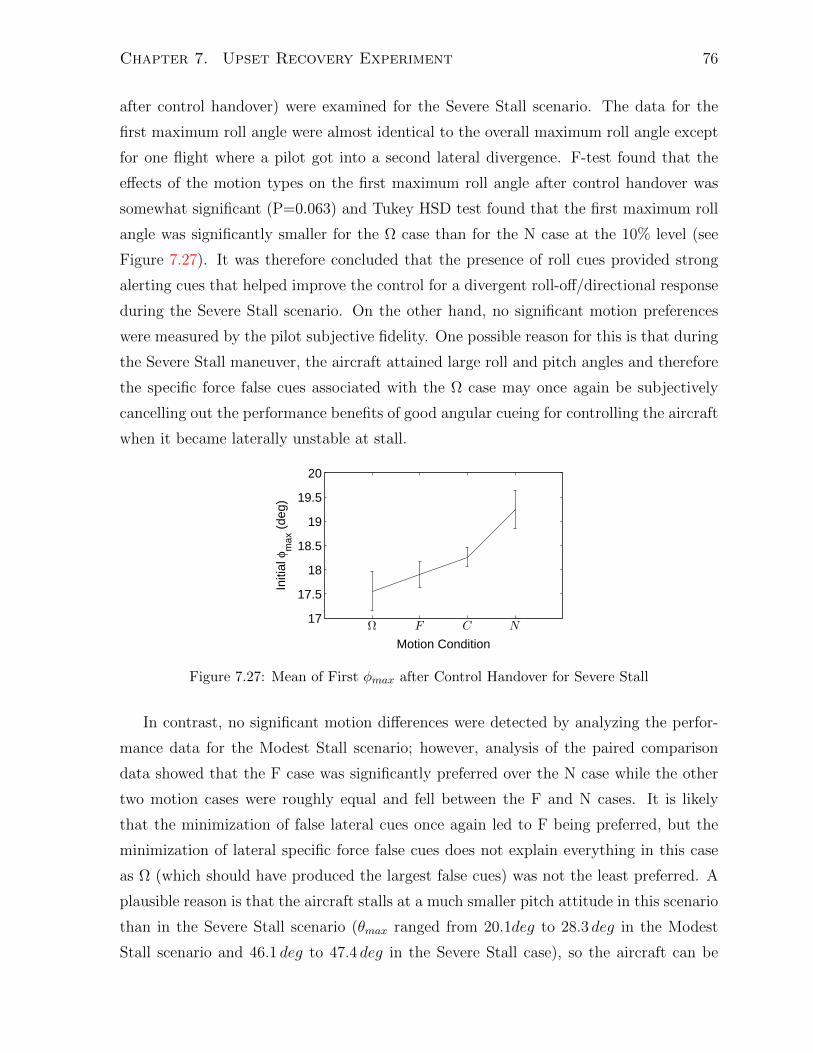
Chapter 7. Upset Recovery Experiment 76
after control handover) were examined for the Severe Stall scenario. The data for the
first maximum roll angle were almost identical to the overall maximum roll angle except
for one flight where a pilot got into a second lateral divergence. F-test found that the
effects of the motion types on the first maximum roll angle after control handover was
somewhat significant (P=0.063) and Tukey HSD test found that the first maximum roll
angle was significantly smaller for the Ω case than for the N case at the 10% level (see
Figure 7.27). It was therefore concluded that the presence of roll cues provided strong
alerting cues that helped improve the control for a divergent roll-off/directional response
during the Severe Stall scenario. On the other hand, no significant motion preferences
were measured by the pilot subjective fidelity. One possible reason for this is that during
the Severe Stall maneuver, the aircraft attained large roll and pitch angles and therefore
the specific force false cues associated with the Ω case may once again be subjectively
cancelling out the performance benefits of good angular cueing for controlling the aircraft
when it became laterally unstable at stall.
17
17.5
18
18.5
19
19.5
20
Ω F C N
Motion Condition
Initi
al φ
max
(de
g)
Figure 7.27: Mean of First φmax after Control Handover for Severe Stall
In contrast, no significant motion differences were detected by analyzing the perfor-
mance data for the Modest Stall scenario; however, analysis of the paired comparison
data showed that the F case was significantly preferred over the N case while the other
two motion cases were roughly equal and fell between the F and N cases. It is likely
that the minimization of false lateral cues once again led to F being preferred, but the
minimization of lateral specific force false cues does not explain everything in this case
as Ω (which should have produced the largest false cues) was not the least preferred. A
plausible reason is that the aircraft stalls at a much smaller pitch attitude in this scenario
than in the Severe Stall scenario (θmax ranged from 20.1deg to 28.3 deg in the Modest
Stall scenario and 46.1 deg to 47.4 deg in the Severe Stall case), so the aircraft can be
Chapter 7. Upset Recovery Experiment 77
easily recovered without entering aggressive roll-off and directional divergence. Conse-
quently, roll and yaw motions were only generated to simulate the dutch-roll introduced
by turbulence for the Modest Stall scenario. During the experiment, the oscillatory roll
and sideslip responses were quickly countered by pilots. As a result, the roll attitude was
generally smaller in this scenario than in the Severe Stall scenario, so the roll cues could
provide useful cueing without generating large lateral specific force false cues. Moreover,
there was not much advantage to the roll cues for reducing the maximum roll angle likely
because the aircraft did not enter roll-off/directional divergence.
For the Pilot Induced Stall scenario, one would probably expect the same results as
those of the Severe Stall scenario since both scenarios involved aerodynamic stalling at
a high pitch attitude; however, no significant motion differences were found in either the
paired comparison data or the performance data for the Pilot Induced Stall scenario. The
differences in the results might be attributed to the differences in the nature of these two
stall conditions. As mentioned in Section 7.1.1, the upset condition for the Severe Stall
scenario was created by pre-programmed control inputs while pilots brought themselves
into a stall for the Pilot Induced Stall case. In general, no two pilots fly the same way
and how well a pilot follows the flight director to induce a stall might change from one
another; therefore, roll-off/directional divergence might only occur in some flights but not
all in the Pilot Induced Stall case. Consequently, the effects of roll cues on controlling
the asymmetric roll-off/directional divergence at stall could not be well determined for
this scenario. Moreover, the subjective preference for the roll cues would depend on
the amount of lateral specific force false cues associated with the roll attitude of each
flight. It is, in fact, interesting to find that although motion cases were not significantly
different, the compromise C case was subjectively rated the best for this scenario.
Overall, the presence of good roll cueing improved lateral control during both a severe
stall and unusual attitude upsets. This confirms with the results presented by Shirley
et al. [24] and Young [46] which suggest that roll cues improved control for unstable
vehicle dynamics. In particular, increasing the fidelity of roll cues at the expense of the
false lateral specific forces led to improvement in pilot performance but not in subjective
fidelity. This is in agreement with the findings of Grant et al. [47]. In another study by
Grant et al. [48], it was found that yaw motion and lateral translational motion improved
performance for a directional disturbance rejection task. Similarly, for the rudder hard-
over event, yaw cues led to the reduction in the dynamic yaw motion during upset;
however, the lateral specific forces did not have an impact on performance and it is likely
Chapter 7. Upset Recovery Experiment 78
because the lateral translational motion examined in the study of Grant et al. [48] were
of high frequency while in the rudder hard-over scenario mainly low frequency lateral
specific forces were generated. In general, pilots rated at least one of the F, Ω, and C
cases higher than the N case for all scenarios. This suggests that the presence of simulator
motion, regardless of the trade-off between translational and rotational motion cues, was
preferred during piloted recovery. Moreover, in all the significant results found in the
performance analysis, the recovery performance was significantly better when simulator
motions were present (F, Ω or C case) than the performance when no simulator motion
was involved (N case). This important finding supports the hypothesis stated at the
beginning of this thesis that simulator motion may be important for UPRT.
Chapter 8
Conclusions
8.1 Summary of Work
In this thesis, a new set of 3-D motion fidelity criteria was defined for coordinated roll
upsets. These criteria were developed based on the modified Sinacori motion fidelity
criteria and Schroeder’s motion fidelity criteria correlated to roll and lateral gains. They
were proposed to estimate the fidelity of general MDAs based on a combination of the
simulator false lateral motion cues, the phase of the intended roll motion, and the gain
of the intended roll motion.
Body frame filters were incorporated into the UTIAS Classical MDA to reduce cross-
coupling among different DOF when simulating large amplitude motion during upset.
Desktop simulations were performed on six different upset scenarios and the results
showed that the elimination of cross-coupling effects did not lead to significant reduc-
tion of motion cue errors. Examination of the simulation results suggests that the upset
scenarios being studied were dominated by low frequency motion and the simulation
of low frequency motion required tilt coordination that did not contain cross-coupling.
Consequently, the motion cue errors reduced by removing cross-coupling effects might be
similar to the errors caused by the additional phase and magnitude errors introduced by
the body frame high-pass filters.
A new adaptive MDA was developed to adapt the gains and frequencies of all high-
pass and low-pass filters numerically without causing undesired oscillations and it has
weights and initial coefficients that can be tuned to adjust the parameter adaptation
rates. The goal of the parameter adaptation is to maximize the fidelity of platform
motion cues during upset recovery simulation. During the tuning of this new MDA, it
79
Chapter 8. Conclusions 80
was determined that for severe upset events both specific force and angular rate cannot
be of medium fidelity simultaneously; therefore, a paired comparison experiment was
performed to analyze the effects of different trade-offs between specific force and angular
rate on subjective motion fidelity and pilot performance during upset recovery. In this
experiment, four different motion conditions, each representing a different type of trade-
off between translational and rotational motion cues, were compared in six different upset
scenarios. All upset scenarios were simulated using the enhanced B-747 roll model and the
simulator motion of all motion cases were generated using the new adaptive MDA. A total
of 18 different sets of motion tuning cases were generated for this experiment. For all these
motion cases, the fidelity before adaptation and the maximum fidelity during adaptation
were evaluated using the modified Sinacori motion fidelity criteria. The fidelity analysis
showed that motion fidelity can be improved using parameter adaptation. In addition,
the roll fidelity of all 18 motion cases were evaluated using both the modified Sinacori
and the new 3-D motion fidelity criteria and it was found that the fidelity estimated
based on solely the magnitude and phase response of the roll high-pass filters could be
overestimated.
Analysis of the subjective paired comparison data found that pilots indicated strong
preference for the minimization of false lateral specific force false cues during large roll
excursions and they preferred angular motion cues when the roll attitude was moderate.
The preference for the minimization of false lateral specific force cues was also observed
in the case of a mild stall where a lateral disturbance was introduced by turbulence
but no aggressive lateral/directional divergence developed. On the other hand, analysis
of the pilot performance data suggests that the presence of roll cues helped improve
lateral control by reducing the first maximum roll angle after control handover as the
aircraft entered a lateral/directional divergence at stall, but no performance benefits were
detected for stall cases where divergent roll-off/directional response did not develop. It
was also found that during unusual attitude upsets, pilots tended to recover with less
aggressive dynamic roll motion when the fidelity of the roll cues was high, and in the
case of rudder hard-over and windshear, pilots tended to recover with less aggressive
dynamic pitch motion when the fidelity of the translational and rotational motion cues
was balanced. Lastly, pilots seemed to recover with a higher normal load factor when no
motion was presented in the Rudder Hard-over event. Overall, pilots indicated preference
for at least one of the three cases with simulator motions over the case with no motion
for all six upset events. Moreover, in all the significant results found in the performance
Chapter 8. Conclusions 81
analysis, the recovery performance was significantly better when simulator motions were
presented (either in terms of best matching specific forces, best matching angular rates,
or best compromise between specific forces and angular rates) than when no motion was
involved. Thus it is suggested by both the subjective fidelity data and the objective
performance data that simulator motion is important for UPRT.
8.2 Future Work
Continuous effort should be put to further improve MDAs for upset recovery simulation.
A possible solution that should be explored is the method of nonlinear scaling. Similar
to the adaptive MDA, nonlinear scaling can be applied to the classical MDA to constrain
aggressive aircraft motions from hitting the actuator limits while allowing moderate mo-
tions to make better use of the motion-base system. The difference being that nonlinear
scaling may be based on maneuver dependent parameters, such as altitude or angle of
attack, instead of the instantaneous simulator states that are used in the adaptive MDA
[25].
Regarding the upset recovery experiment, future work should include constructing a
set of measurements that defines “best specific forces”, “best angular rates” and “best
compromise between specific forces and angular rates” more precisely for tuning motion
parameters for the adaptive MDA. In addition, MDAs and their tuning method should be
improved to account for the tradeoff between false lateral motion cues and onset rotational
motion cues when simulating roll attitude excursions at upset. Finally, performance
criteria should be clearly defined in order to more accurately measure pilot performance
during upset recovery.
Bibliography
[1] J. Burki-Cohen and A. L. Sparko. Airplane upset prevention research needs. In AIAA
Modelling and Simulation Technologies Conference and Exhibit, number AIAA 2008-
6871, Honolulu, HI, August 2008.
[2] J. E. Wilborn and J. V. Foster. Defining commercial transport loss-of-control: A
quantitative approach. In AIAA Atmospheric Flight Mechanics Conference and
Exhibit, number AIAA 2004-4811, Providence, RI, August 2004.
[3] A. A. Lambregts, G. Nesemeier, J. E. Wilborn, and R. L. Newman. Airplane up-
sets: Old problem, new issues. In AIAA Modelling and Simulation Technologies
Conference and Exhibit, number AIAA 2008-6867, Honolulu, HI, August 2008.
[4] The Boeing Company. Statistical summary of commercial jet airplane accidents:
Worldwide operations 1959-2008. Technical report, Boeing Commercial Airplanes,
Seattle, WA, July 2009.
[5] The Boeing Company. Statistical summary of commercial jet airplane accidents:
Worldwide operations 1959-2009. Technical report, Boeing Commercial Airplanes,
Seattle, WA, July 2010.
[6] The Boeing Company. Statistical summary of commercial jet airplane accidents:
Worldwide operations 1959-2010. Technical report, Boeing Commercial Airplanes,
Seattle, WA, June 2011.
[7] The Boeing Company. Statistical summary of commercial jet airplane accidents:
Worldwide operations 1959-2011. Technical report, Boeing Commercial Airplanes,
Seattle, WA, July 2012.
82
Bibliography 83
[8] C. M. Belcastro. Aircraft loss of control: Analysis and requirements for future
safety-critical systems and their validation. In Proceedings of the 8th Asian Control
Conference, pages 399–406, Kaohsiung, May 2011.
[9] D. Carbaugh and L. Rockliff. Airplane upset recovery: Training aid, revision 1.
August 2004.
[10] S. F. Liu. Ground-based simulation of airplane upset using an enhanced flight model.
Master’s thesis, University of Toronto Institute for Aerospace Studies, 2010.
[11] V. J. Gawron. Airplane upset training evaluation report. NASA/CR 2002-211405,
Veridian Engineering, Buffalo, NY, May 2002.
[12] Bureau d’Enquetes et d’Analyses. Safety investigation following the accident on 1ST
June 2009 to the Airbus A300-203, flight AF447. Technical report, Le Bourget, July
2012.
[13] National Transportation Safety Board. Loss of control on approach, Colgan Air,
Inc., Operating as Continental Connection Flight 3407, Bombardier DHC-8-400,
N200WQ, Clarence Center, New York, February 12, 2009. Technical Report
NTSB/AAR-10/01, NTSB, Washington, DC, February 2010.
[14] National Transportation Safety Board. Crash of Pinnacle Airlines Flight 3701, Bom-
bardier CL-600-2B19, N8396A, Jefferson City, Missouri, October 14, 2004. Technical
Report NTSB/AAR-07/01, NTSB, Washington, DC, January 2007.
[15] G. H. Shah, K. Cunningham, J. V. Foster, C. M. Fremaux, E. C. Stewart, J. E.
Wilborn, W. Gato, and D. W. Pratt. Wind-tunnel investigation of commercial
transport aircraft aerodynamics at extreme flight conditions. In World Aviation
Congress and Display, number SAE 2002-01-2912, Phoenix, AZ, November 2002.
[16] K. Cunningham, J. V. Foster, G. H. Shah, E. C. Stewart, R. N. Ventura, R. A.
Rivers, J. E. Wilborn, and W. Gato. Simulation study of flap effects on a commercial
transport airplane in upset conditions. In AIAA Atmospheric Flight Mechanics
Conference and Exhibit, number AIAA 2005-5908, San Francisco, CA, August 2005.
[17] J. V. Foster, K. Cunningham, C. M. Fremaux, G. H. Shah, E. C. Stewart, R. A.
Rivers, J. E. Wilborn, and W. Gato. Dynamics modeling and simulation of large
Bibliography 84
transport airplanes in upset conditions. In AIAA Guidance Navigation and Control
Conference and Exhibit, number AIAA 2005-5933, San Francisco, CA, August 2005.
[18] N. B. Abramov, M. G. Goman, A. N. Khrabrov, E. N. Kolesnoikov, L. Fucke, B. Soe-
marwoto, and H. Smaili. Pushing ahead - SUPRA airplane model for upset recov-
ery. In AIAA Modeling and Simulation Technologies Conference, number AIAA
2012-4631, Minneapolis, MN, August 2012.
[19] J. Burki-Cohen A. L. Sparko and T. H. Go. Transfer of training from a full-flight
simulator vs. a high level flight training device with a dynamic seat. In AIAA Mod-
elling and Simulation Technologies Conference, number AIAA 2010-8218, Toronto,
ON, August 2010.
[20] M. D. White and G. E. Cooper. A piloted simulation study of operational aspects
of the stall pitch-up. NASA TN D-4071, July 1967.
[21] H. P. Bergeron, J. J. Adams, and G. J. Hurt, Jr. The effects of motion cues and
motion scaling on one- and two-axis compensatory control tasks. NASA TN D-6110,
January 1971.
[22] J. L. Meiry. The Vesitbular System and Human Dynamic Space Orientation. T-65-1,
Massachusetts Institute of Technology, Man-Vehicle Control Laboratory, 1965.
[23] R. L. Stapleford, R. A. Peters, and F. R. Alex. Experiments and a model for pilot
dynamics with visual and motion inputs. NASA CR- 1325, May 1969.
[24] R. S. Shirley and L. R. Young. Motion cues in man-vehicle control: Effects of
roll-motion cues on human operator’s behavior in compensatory systems with dis-
turbance inputs. IEEE Transactions on Man-Machine System, MMS-9(4):121–128,
1968.
[25] W. W. Chung. A preliminary investigation of achievable motion cueing in ground-
based flight simulators for upset recovery maneuvers. In AIAA Modeling and Sim-
ulation Technologies Conference and Exhibit, number AIAA 2008-6868, Honolulu,
HI, August 2008. AIAA.
[26] J. A. Schroeder. Helicopter flight simulation motion platform requirements.
NASA/TP 1999-208766, Moffett Field, CA, July 1999.
Bibliography 85
[27] L. E. Zaichik, Y. P. Yashin, P. A. Desyatnik, and H. Smaili. Some aspects of upset
recovering simulation on hexapod simulators. In AIAA Modeling and Simulation
Technologies Conference, number AIAA 2012-4949, Minneapolis, MN, August 2012.
[28] J. Field, M. Roza, and H. Smaili. Developing upset cueing for conventional flight
simulators. In AIAA Modeling and Simulation Technologies Conference, number
AIAA 2012-4948, Minneapolis, MN, August 2012.
[29] C. R. Hanke and D. R. Nordwall. The simulation of a jumbo jet transport aircraft
Vol. II: Modeling data. NASA-CR- 114494, D6-30643, The Boeing Company/NASA,
Wichita, KS, September 1970.
[30] P. R. Grant. The Development of a Tuning Paradigm for Flight Simulator Mo-
tion Drive Algorithms, Volume I. PhD thesis, University of Toronto Institute for
Aerospace Studies, 1996.
[31] A. R. Naseri. Improvement of the UTIAS adaptive motion drive algorithm. Master’s
thesis, University of Toronto Institute for Aerospace Studies, 2006.
[32] L. D. Reid and M. A. Nahon. Flight simulation motion-base drive algorithms: Part 1
- Developing and testing the equations. Technical Report No. 296, UTIAS, December
1985.
[33] J. A. Schroeder and P. R. Grant. Pilot behavioral observations in motion flight
simulation. In AIAA Modelling and Simulation Technologies Conference, number
AIAA 2010-8353, Toronto, ON, August 2010.
[34] L. D. Reid and M. A. Nahon. Flight simulation motion-base drive algorithms: Part
2 - Selecting the system parameters. Technical Report No. 307, UTIAS, January
1986.
[35] L. D. Reid and M. A. Nahon. Flight simulation motion-base drive algorithms: Part
3 - Pilot evaluations. Technical Report No. 319, UTIAS, December 1986.
[36] R. V. Parrish and D. J. Martin, Jr. Comparison of a linear and a nonlinear washout
for motion simulators utilizing objective and subjective data from CTOL transport
landing approaches. NASA TN D-8157, June 1976.
Bibliography 86
[37] G. J. O’Toole. An investigation of the UTIAS Adaptive Washout Algorithm. Mas-
ter’s thesis, University of Toronto Institute for Aerospace Studies, 1995.
[38] J. B. Sinacori. The determination of some requirements for a helicopter flight re-
search simulation facility. NASA CR 152066, September 1977.
[39] G. L. Greig. Masking of Motion Cues by Random Motion: Comparison of Human
Performance With a Signal Detection Model. PhD thesis, University of Toronto
Institute for Aerospace Studies, 1988.
[40] C. Jiang. Buffet simulation of the UTIAS Flight Research Simulator. Technical
report, University of Toronto, April 2012.
[41] K. A. Butler. Some problems in paired comparisons and goodness of fit for logistic
regression. PhD thesis, Simon Fraser University, Burnaby, BC, 1997.
[42] H. A. David. The Method of Paired Comparisons. Oxford University Press, New
York, NY, 1988.
[43] R. R. Davidson and R. J. Beaver. On extending the Bradley-Terry model to incor-
porate within-pair order effects. Biometrics, 33(4):693–702, 1977.
[44] R. R. Davidson. On extending the Bradley-Terry model to accommodate ties in
paired comparison experiments. Technical Report No. 37, Florida State University,
August 1969.
[45] B. J. Winer, D. R. Brown, and K. M. Michels. Statistical Principles in Experimental
Design. McGraw Hill, Boston, MA, 3rd edition, 1991.
[46] L. R. Young. Some effects of motion cues on manual tracking. AIAA Journal of
Spacecraft, 4(10):1300–1303, 1967.
[47] P. R. Grant, M. Blommer, B. Artz, and J. Greenberg. Analysing classes of motion
drive algorithms based on paired comparison techniques. Vehicle System Dynamics,
47(9):1075–1093, 2009.
[48] P. R. Grant, B. Yam, R. Hosman, and J. A. Schroeder. Effect of simulator motion
on pilot behavior and perception. AIAA Journal of Aircraft, 43(6):1914–1924, 2006.
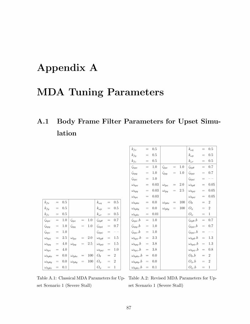
Appendix A
MDA Tuning Parameters
A.1 Body Frame Filter Parameters for Upset Simu-
lation
kfx = 0.5 kωq = 0.5
kfy = 0.5 kωp = 0.5
kfz = 0.5 kωr = 0.5
ζhpx = 1.0 ζlpx = 1.0 ζhpθ = 0.7
ζhpy = 1.0 ζlpy = 1.0 ζhpφ = 0.7
ζhpz = 1.0 ζhpψ = – –
ωhpx = 2.5 ωlpx = 2.0 ωhpθ = 1.5
ωhpy = 4.0 ωlpy = 2.5 ωhpφ = 1.5
ωhpz = 4.0 ωhpψ = 1.0
ωhpbx = 0.0 ωlpbx = 100 Oθ = 2
ωhpby = 0.0 ωlpby = 100 Oφ = 2
ωhpbz = 0.1 Oψ = 1
Table A.1: Classical MDA Parameters for Up-
set Scenario 1 (Severe Stall)
kfx = 0.5 kωq = 0.5
kfy = 0.5 kωp = 0.5
kfz = 0.5 kωr = 0.5
ζhpx = 1.0 ζlpx = 1.0 ζhpθ = 0.7
ζhpy = 1.0 ζlpy = 1.0 ζhpφ = 0.7
ζhpz = 1.0 ζhpψ = – –
ωhpx = 0.03 ωlpx = 2.0 ωhpθ = 0.05
ωhpy = 0.03 ωlpy = 2.5 ωhpφ = 0.05
ωhpz = 0.03 ωhpψ = 0.05
ωhpbx = 0.0 ωlpbx = 100 Oθ = 2
ωhpby = 0.0 ωlpby = 100 Oφ = 2
ωhpbz = 0.01 Oψ = 1
ζhpx b = 1.0 ζhpθ b = 0.7
ζhpy b = 1.0 ζhpφ b = 0.7
ζhpz b = 1.0 ζhpψ b = – –
ωhpx b = 2.3 ωhpθ b = 1.3
ωhpy b = 3.8 ωhpφ b = 1.3
ωhpz b = 3.8 ωhpψ b = 0.8
ωhpbx b = 0.0 Oθ b = 2
ωhpby b = 0.0 Oφ b = 2
ωhpbz b = 0.1 Oψ b = 1
Table A.2: Revised MDA Parameters for Up-
set Scenario 1 (Severe Stall)
87
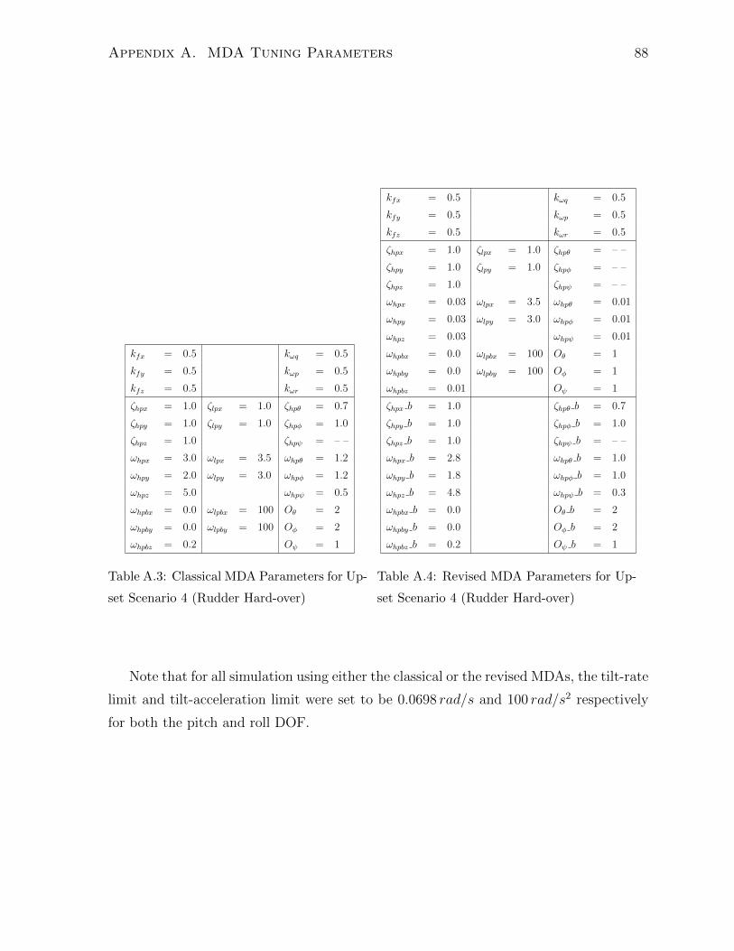
Appendix A. MDA Tuning Parameters 88
kfx = 0.5 kωq = 0.5
kfy = 0.5 kωp = 0.5
kfz = 0.5 kωr = 0.5
ζhpx = 1.0 ζlpx = 1.0 ζhpθ = 0.7
ζhpy = 1.0 ζlpy = 1.0 ζhpφ = 1.0
ζhpz = 1.0 ζhpψ = – –
ωhpx = 3.0 ωlpx = 3.5 ωhpθ = 1.2
ωhpy = 2.0 ωlpy = 3.0 ωhpφ = 1.2
ωhpz = 5.0 ωhpψ = 0.5
ωhpbx = 0.0 ωlpbx = 100 Oθ = 2
ωhpby = 0.0 ωlpby = 100 Oφ = 2
ωhpbz = 0.2 Oψ = 1
Table A.3: Classical MDA Parameters for Up-
set Scenario 4 (Rudder Hard-over)
kfx = 0.5 kωq = 0.5
kfy = 0.5 kωp = 0.5
kfz = 0.5 kωr = 0.5
ζhpx = 1.0 ζlpx = 1.0 ζhpθ = – –
ζhpy = 1.0 ζlpy = 1.0 ζhpφ = – –
ζhpz = 1.0 ζhpψ = – –
ωhpx = 0.03 ωlpx = 3.5 ωhpθ = 0.01
ωhpy = 0.03 ωlpy = 3.0 ωhpφ = 0.01
ωhpz = 0.03 ωhpψ = 0.01
ωhpbx = 0.0 ωlpbx = 100 Oθ = 1
ωhpby = 0.0 ωlpby = 100 Oφ = 1
ωhpbz = 0.01 Oψ = 1
ζhpx b = 1.0 ζhpθ b = 0.7
ζhpy b = 1.0 ζhpφ b = 1.0
ζhpz b = 1.0 ζhpψ b = – –
ωhpx b = 2.8 ωhpθ b = 1.0
ωhpy b = 1.8 ωhpφ b = 1.0
ωhpz b = 4.8 ωhpψ b = 0.3
ωhpbx b = 0.0 Oθ b = 2
ωhpby b = 0.0 Oφ b = 2
ωhpbz b = 0.2 Oψ b = 1
Table A.4: Revised MDA Parameters for Up-
set Scenario 4 (Rudder Hard-over)
Note that for all simulation using either the classical or the revised MDAs, the tilt-rate
limit and tilt-acceleration limit were set to be 0.0698 rad/s and 100 rad/s2 respectively
for both the pitch and roll DOF.
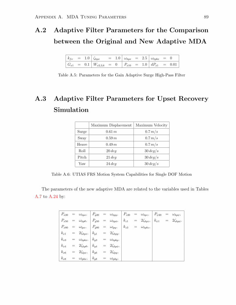
Appendix A. MDA Tuning Parameters 89
A.2 Adaptive Filter Parameters for the Comparison
between the Original and New Adaptive MDA
kfx = 1.0 ζhpx = 1.0 ωhpx = 2.5 ωhpbx = 0
Gx1 = 0.1 Wx2,3,6 = 0 Px10 = 1.0 dPx1 = 0.01
Table A.5: Parameters for the Gain Adaptive Surge High-Pass Filter
A.3 Adaptive Filter Parameters for Upset Recovery
Simulation
Maximum Displacement Maximum Velocity
Surge 0.61m 0.7m/s
Sway 0.59m 0.7m/s
Heave 0.49m 0.7m/s
Roll 20 deg 30 deg/s
Pitch 21 deg 30 deg/s
Yaw 24 deg 30 deg/s
Table A.6: UTIAS FRS Motion System Capabilities for Single DOF Motion
The parameters of the new adaptive MDA are related to the variables used in Tables
A.7 to A.24 by:
Px20 = ωhpx, Py20 = ωhpy, Pz20 = ωhpz, Pψ20 = ωhpψ,
Px50 = ωhpθ, Py50 = ωhpφ, kz1 = 2ζhpz, kψ1 = 2ζhpψ.
Px80 = ωlpx, Py80 = ωlpy, kz3 = ωhpbz,
kx1 = 2ζhpx, ky1 = 2ζhpy,
kx3 = ωhpbx, ky3 = ωhpby,
kx4 = 2ζhpθ, ky4 = 2ζhpφ,
kx6 = 2ζlpx, ky6 = 2ζlpy,
kx8 = ωlpbx, ky8 = ωlpby,

Appendix A. MDA Tuning Parameters 90
Surge/Pitch Sway/Roll
kfx = 0.5 kfy = 0.5
kωq = 0.5 kωp = 0.5
ζhpx = 1.0 ζhpy = 1.0
ωhpx = 4.0 ωhpy = 4.0
ωhpbx = 0 ωhpby = 0
ζlpx = 1.0 ζlpy = 1.0
ωlpx = 2.0 ωlpy = 3.0
ωlpbx = 100 ωlpby = 100
ζhpθ = 0.7 ζhpφ = 0.7
ωhpθ = 3.0 ωhpφ = 3.0
Gx1 = 0 Gy1 = 0
Gx2 = 0 Gy2 = 0.01
Gx4 = 0 Gy4 = 0
Gx5 = 0 Gy5 = 0
Gx7 = 0 Gy7 = 0
Gx8 = 0.03 Gy8 = 0.3
Wx0 = 0.5 Wy0 = 0.03
Wx1 = 0 Wy1 = 0
Wx2 = 0 Wy2 = 0
Wx3 = 0 Wy3 = 0
Wx4 = 0 Wy4 = 0
Wx5 = 0 Wy5 = 0
Wx6 = 0 Wy6 = 0
Wx7 = 0 Wy7 = 3.0
Wx9 = 0 Wy9 = 0
Wx10 = 0 Wy10 = 0
Wx12 = 0 Wy12 = 0
Wx13 = 3.0 Wy13 = 0.3
Px10 = 1.0 Py10 = 1.0
Px40 = 1.0 Py40 = 1.0
Px70 = 1.0 Py70 = 1.0
∆Px1 = 0.01 ∆Py1 = 0.01
∆Px2 = 0.01 ∆Py2 = 0.01
∆Px4 = 0.01 ∆Py4 = 0.01
∆Px5 = 0.01 ∆Py5 = 0.01
∆Px7 = 0.01 ∆Py7 = 0.01
∆Px8 = 0.001 ∆Py8 = 0.001
Heave Yaw
kfz = 0.5 kωr = 0.5
ζhpz = 1.0 ζhpψ = 1.0
ωhpz = 4.0 ωhpψ = 0.1
ωhpbz = 0.1 Gψ1 = 0
Gz1 = 0 Gψ2 = 0
Gz2 = 0 Wψ0 = 0
Wz0 = 0 Wψ1 = 0
Wz1 = 0 Wψ2 = 0
Wz2 = 0 Wψ3 = 0
Wz3 = 0 Wψ4 = 0
Wz4 = 0 Pψ10 = 1.0
Pz10 = 1.0 ∆Pψ1 = 0.01
∆Pz1 = 0.01 ∆Pψ2 = 0.01
∆Pz2 = 0.01
Table A.7: Scenario 1 - F
Surge/Pitch Sway/Roll
kfx = 0.4 kfy = 0.4
kωq = 0.5 kωp = 0.5
ζhpx = 1.0 ζhpy = 1.0
ωhpx = 5.0 ωhpy = 5.0
ωhpbx = 0 ωhpby = 0
ζlpx = 1.0 ζlpy = 1.0
ωlpx = 0.1 ωlpy = 0
ωlpbx = 100 ωlpby = 100
ζhpθ = 0.7 ζhpφ = 0.7
ωhpθ = 0.2 ωhpφ = 0.2
Gx1 = 0 Gy1 = 0
Gx2 = 0 Gy2 = 0
Gx4 = 0 Gy4 = 0
Gx5 = 0.001 Gy5 = 0.05
Gx7 = 0 Gy7 = 0
Gx8 = 0 Gy8 = 0
Wx0 = 0 Wy0 = 0
Wx1 = 0.03 Wy1 = 0.03
Wx2 = 0 Wy2 = 0
Wx3 = 0 Wy3 = 0
Wx4 = 0 Wy4 = 0
Wx5 = 0 Wy5 = 0
Wx6 = 0 Wy6 = 0
Wx7 = 0 Wy7 = 0
Wx9 = 0 Wy9 = 0
Wx10 = 15.0 Wy10 = 5.0
Wx12 = 0 Wy12 = 0
Wx13 = 0 Wy13 = 0
Px10 = 1.0 Py10 = 1.0
Px40 = 1.0 Py40 = 1.0
Px70 = 1.0 Py70 = 1.0
∆Px1 = 0.01 ∆Py1 = 0.01
∆Px2 = 0.01 ∆Py2 = 0.01
∆Px4 = 0.01 ∆Py4 = 0.01
∆Px5 = 0.001 ∆Py5 = 0.01
∆Px7 = 0.01 ∆Py7 = 0.01
∆Px8 = 0.01 ∆Py8 = 0.01
Heave Yaw
kfz = 0.4 kωr = 0.5
ζhpz = 1.0 ζhpψ = 1.0
ωhpz = 5.0 ωhpψ = 0.1
ωhpbz = 0.1 Gψ1 = 0
Gz1 = 0 Gψ2 = 0.05
Gz2 = 0 Wψ0 = 0.01
Wz0 = 0 Wψ1 = 0
Wz1 = 0 Wψ2 = 0
Wz2 = 0 Wψ3 = 0
Wz3 = 0 Wψ4 = 0.1
Wz4 = 0 Pψ10 = 1.0
Pz10 = 1.0 ∆Pψ1 = 0.01
∆Pz1 = 0.01 ∆Pψ2 = 0.001
∆Pz2 = 0.01
Table A.8: Scenario 1 - Ω
Surge/Pitch Sway/Roll
kfx = 0.45 kfy = 0.45
kωq = 0.45 kωp = 0.45
ζhpx = 1.0 ζhpy = 1.0
ωhpx = 4.0 ωhpy = 4.0
ωhpbx = 0 ωhpby = 0
ζlpx = 1.0 ζlpy = 1.0
ωlpx = 0.75 ωlpy = 1.0
ωlpbx = 100 ωlpby = 100
ζhpθ = 0.7 ζhpφ = 0.7
ωhpθ = 1.0 ωhpφ = 1.0
Gx1 = 0 Gy1 = 0
Gx2 = 0 Gy2 = 0
Gx4 = 0 Gy4 = 0
Gx5 = 0.01 Gy5 = 0.05
Gx7 = 0 Gy7 = 0
Gx8 = 0.008 Gy8 = 0.15
Wx0 = 0.05 Wy0 = 0.002
Wx1 = 0.01 Wy1 = 0.01
Wx2 = 0 Wy2 = 0
Wx3 = 0 Wy3 = 0
Wx4 = 0 Wy4 = 0
Wx5 = 0 Wy5 = 0
Wx6 = 0 Wy6 = 0
Wx7 = 0 Wy7 = 0
Wx9 = 0 Wy9 = 0
Wx10 = 1.0 Wy10 = 0.001
Wx12 = 0 Wy12 = 0
Wx13 = 5.0 Wy13 = 0.001
Px10 = 1.0 Py10 = 1.0
Px40 = 1.0 Py40 = 1.0
Px70 = 1.0 Py70 = 1.0
∆Px1 = 0.01 ∆Py1 = 0.01
∆Px2 = 0.01 ∆Py2 = 0.01
∆Px4 = 0.01 ∆Py4 = 0.01
∆Px5 = 0.001 ∆Py5 = 0.01
∆Px7 = 0.01 ∆Py7 = 0.01
∆Px8 = 0.001 ∆Py8 = 0.001
Heave Yaw
kfz = 0.45 kωr = 0.45
ζhpz = 1.0 ζhpψ = 1.0
ωhpz = 4.0 ωhpψ = 0.3
ωhpbz = 0.1 Gψ1 = 0
Gz1 = 0 Gψ2 = 0.3
Gz2 = 0 Wψ0 = 0.005
Wz0 = 0 Wψ1 = 0
Wz1 = 0 Wψ2 = 0
Wz2 = 0 Wψ3 = 0
Wz3 = 0 Wψ4 = 0.01
Wz4 = 0 Pψ10 = 1.0
Pz10 = 1.0 ∆Pψ1 = 0.01
∆Pz1 = 0.01 ∆Pψ2 = 0.001
∆Pz2 = 0.01
Table A.9: Scenario 1 - C
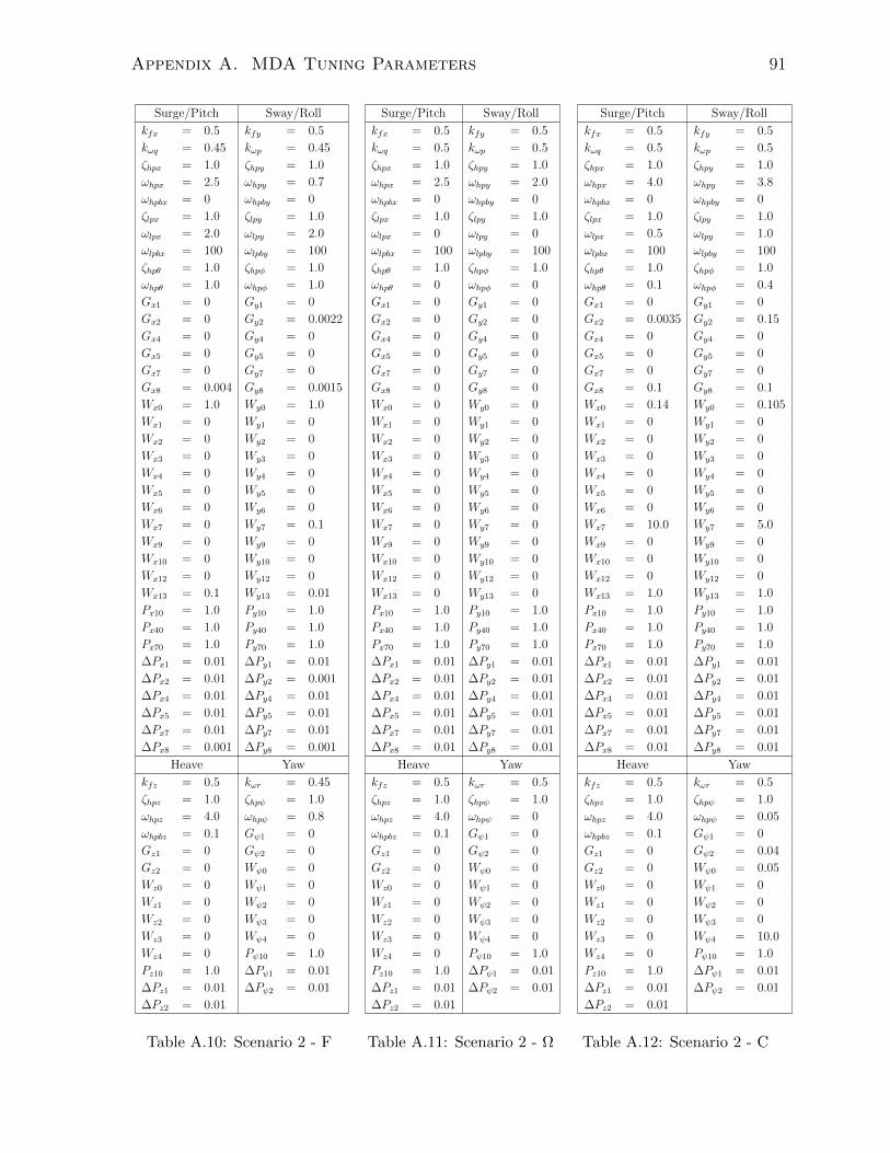
Appendix A. MDA Tuning Parameters 91
Surge/Pitch Sway/Roll
kfx = 0.5 kfy = 0.5
kωq = 0.45 kωp = 0.45
ζhpx = 1.0 ζhpy = 1.0
ωhpx = 2.5 ωhpy = 0.7
ωhpbx = 0 ωhpby = 0
ζlpx = 1.0 ζlpy = 1.0
ωlpx = 2.0 ωlpy = 2.0
ωlpbx = 100 ωlpby = 100
ζhpθ = 1.0 ζhpφ = 1.0
ωhpθ = 1.0 ωhpφ = 1.0
Gx1 = 0 Gy1 = 0
Gx2 = 0 Gy2 = 0.0022
Gx4 = 0 Gy4 = 0
Gx5 = 0 Gy5 = 0
Gx7 = 0 Gy7 = 0
Gx8 = 0.004 Gy8 = 0.0015
Wx0 = 1.0 Wy0 = 1.0
Wx1 = 0 Wy1 = 0
Wx2 = 0 Wy2 = 0
Wx3 = 0 Wy3 = 0
Wx4 = 0 Wy4 = 0
Wx5 = 0 Wy5 = 0
Wx6 = 0 Wy6 = 0
Wx7 = 0 Wy7 = 0.1
Wx9 = 0 Wy9 = 0
Wx10 = 0 Wy10 = 0
Wx12 = 0 Wy12 = 0
Wx13 = 0.1 Wy13 = 0.01
Px10 = 1.0 Py10 = 1.0
Px40 = 1.0 Py40 = 1.0
Px70 = 1.0 Py70 = 1.0
∆Px1 = 0.01 ∆Py1 = 0.01
∆Px2 = 0.01 ∆Py2 = 0.001
∆Px4 = 0.01 ∆Py4 = 0.01
∆Px5 = 0.01 ∆Py5 = 0.01
∆Px7 = 0.01 ∆Py7 = 0.01
∆Px8 = 0.001 ∆Py8 = 0.001
Heave Yaw
kfz = 0.5 kωr = 0.45
ζhpz = 1.0 ζhpψ = 1.0
ωhpz = 4.0 ωhpψ = 0.8
ωhpbz = 0.1 Gψ1 = 0
Gz1 = 0 Gψ2 = 0
Gz2 = 0 Wψ0 = 0
Wz0 = 0 Wψ1 = 0
Wz1 = 0 Wψ2 = 0
Wz2 = 0 Wψ3 = 0
Wz3 = 0 Wψ4 = 0
Wz4 = 0 Pψ10 = 1.0
Pz10 = 1.0 ∆Pψ1 = 0.01
∆Pz1 = 0.01 ∆Pψ2 = 0.01
∆Pz2 = 0.01
Table A.10: Scenario 2 - F
Surge/Pitch Sway/Roll
kfx = 0.5 kfy = 0.5
kωq = 0.5 kωp = 0.5
ζhpx = 1.0 ζhpy = 1.0
ωhpx = 2.5 ωhpy = 2.0
ωhpbx = 0 ωhpby = 0
ζlpx = 1.0 ζlpy = 1.0
ωlpx = 0 ωlpy = 0
ωlpbx = 100 ωlpby = 100
ζhpθ = 1.0 ζhpφ = 1.0
ωhpθ = 0 ωhpφ = 0
Gx1 = 0 Gy1 = 0
Gx2 = 0 Gy2 = 0
Gx4 = 0 Gy4 = 0
Gx5 = 0 Gy5 = 0
Gx7 = 0 Gy7 = 0
Gx8 = 0 Gy8 = 0
Wx0 = 0 Wy0 = 0
Wx1 = 0 Wy1 = 0
Wx2 = 0 Wy2 = 0
Wx3 = 0 Wy3 = 0
Wx4 = 0 Wy4 = 0
Wx5 = 0 Wy5 = 0
Wx6 = 0 Wy6 = 0
Wx7 = 0 Wy7 = 0
Wx9 = 0 Wy9 = 0
Wx10 = 0 Wy10 = 0
Wx12 = 0 Wy12 = 0
Wx13 = 0 Wy13 = 0
Px10 = 1.0 Py10 = 1.0
Px40 = 1.0 Py40 = 1.0
Px70 = 1.0 Py70 = 1.0
∆Px1 = 0.01 ∆Py1 = 0.01
∆Px2 = 0.01 ∆Py2 = 0.01
∆Px4 = 0.01 ∆Py4 = 0.01
∆Px5 = 0.01 ∆Py5 = 0.01
∆Px7 = 0.01 ∆Py7 = 0.01
∆Px8 = 0.01 ∆Py8 = 0.01
Heave Yaw
kfz = 0.5 kωr = 0.5
ζhpz = 1.0 ζhpψ = 1.0
ωhpz = 4.0 ωhpψ = 0
ωhpbz = 0.1 Gψ1 = 0
Gz1 = 0 Gψ2 = 0
Gz2 = 0 Wψ0 = 0
Wz0 = 0 Wψ1 = 0
Wz1 = 0 Wψ2 = 0
Wz2 = 0 Wψ3 = 0
Wz3 = 0 Wψ4 = 0
Wz4 = 0 Pψ10 = 1.0
Pz10 = 1.0 ∆Pψ1 = 0.01
∆Pz1 = 0.01 ∆Pψ2 = 0.01
∆Pz2 = 0.01
Table A.11: Scenario 2 - Ω
Surge/Pitch Sway/Roll
kfx = 0.5 kfy = 0.5
kωq = 0.5 kωp = 0.5
ζhpx = 1.0 ζhpy = 1.0
ωhpx = 4.0 ωhpy = 3.8
ωhpbx = 0 ωhpby = 0
ζlpx = 1.0 ζlpy = 1.0
ωlpx = 0.5 ωlpy = 1.0
ωlpbx = 100 ωlpby = 100
ζhpθ = 1.0 ζhpφ = 1.0
ωhpθ = 0.1 ωhpφ = 0.4
Gx1 = 0 Gy1 = 0
Gx2 = 0.0035 Gy2 = 0.15
Gx4 = 0 Gy4 = 0
Gx5 = 0 Gy5 = 0
Gx7 = 0 Gy7 = 0
Gx8 = 0.1 Gy8 = 0.1
Wx0 = 0.14 Wy0 = 0.105
Wx1 = 0 Wy1 = 0
Wx2 = 0 Wy2 = 0
Wx3 = 0 Wy3 = 0
Wx4 = 0 Wy4 = 0
Wx5 = 0 Wy5 = 0
Wx6 = 0 Wy6 = 0
Wx7 = 10.0 Wy7 = 5.0
Wx9 = 0 Wy9 = 0
Wx10 = 0 Wy10 = 0
Wx12 = 0 Wy12 = 0
Wx13 = 1.0 Wy13 = 1.0
Px10 = 1.0 Py10 = 1.0
Px40 = 1.0 Py40 = 1.0
Px70 = 1.0 Py70 = 1.0
∆Px1 = 0.01 ∆Py1 = 0.01
∆Px2 = 0.01 ∆Py2 = 0.01
∆Px4 = 0.01 ∆Py4 = 0.01
∆Px5 = 0.01 ∆Py5 = 0.01
∆Px7 = 0.01 ∆Py7 = 0.01
∆Px8 = 0.01 ∆Py8 = 0.01
Heave Yaw
kfz = 0.5 kωr = 0.5
ζhpz = 1.0 ζhpψ = 1.0
ωhpz = 4.0 ωhpψ = 0.05
ωhpbz = 0.1 Gψ1 = 0
Gz1 = 0 Gψ2 = 0.04
Gz2 = 0 Wψ0 = 0.05
Wz0 = 0 Wψ1 = 0
Wz1 = 0 Wψ2 = 0
Wz2 = 0 Wψ3 = 0
Wz3 = 0 Wψ4 = 10.0
Wz4 = 0 Pψ10 = 1.0
Pz10 = 1.0 ∆Pψ1 = 0.01
∆Pz1 = 0.01 ∆Pψ2 = 0.01
∆Pz2 = 0.01
Table A.12: Scenario 2 - C
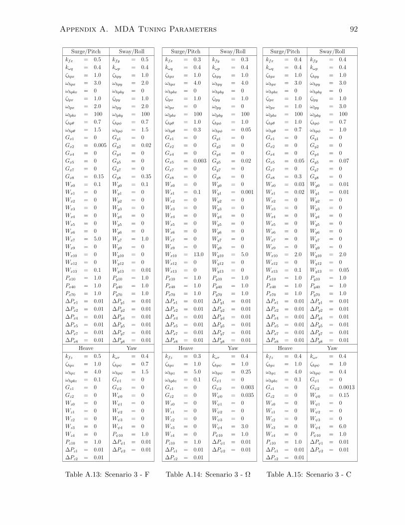
Appendix A. MDA Tuning Parameters 92
Surge/Pitch Sway/Roll
kfx = 0.5 kfy = 0.5
kωq = 0.4 kωp = 0.4
ζhpx = 1.0 ζhpy = 1.0
ωhpx = 3.0 ωhpy = 2.0
ωhpbx = 0 ωhpby = 0
ζlpx = 1.0 ζlpy = 1.0
ωlpx = 2.0 ωlpy = 2.0
ωlpbx = 100 ωlpby = 100
ζhpθ = 0.7 ζhpφ = 0.7
ωhpθ = 1.5 ωhpφ = 1.5
Gx1 = 0 Gy1 = 0
Gx2 = 0.005 Gy2 = 0.02
Gx4 = 0 Gy4 = 0
Gx5 = 0 Gy5 = 0
Gx7 = 0 Gy7 = 0
Gx8 = 0.15 Gy8 = 0.35
Wx0 = 0.1 Wy0 = 0.1
Wx1 = 0 Wy1 = 0
Wx2 = 0 Wy2 = 0
Wx3 = 0 Wy3 = 0
Wx4 = 0 Wy4 = 0
Wx5 = 0 Wy5 = 0
Wx6 = 0 Wy6 = 0
Wx7 = 5.0 Wy7 = 1.0
Wx9 = 0 Wy9 = 0
Wx10 = 0 Wy10 = 0
Wx12 = 0 Wy12 = 0
Wx13 = 0.1 Wy13 = 0.01
Px10 = 1.0 Py10 = 1.0
Px40 = 1.0 Py40 = 1.0
Px70 = 1.0 Py70 = 1.0
∆Px1 = 0.01 ∆Py1 = 0.01
∆Px2 = 0.01 ∆Py2 = 0.01
∆Px4 = 0.01 ∆Py4 = 0.01
∆Px5 = 0.01 ∆Py5 = 0.01
∆Px7 = 0.01 ∆Py7 = 0.01
∆Px8 = 0.01 ∆Py8 = 0.01
Heave Yaw
kfz = 0.5 kωr = 0.4
ζhpz = 1.0 ζhpψ = 0.7
ωhpz = 4.0 ωhpψ = 1.5
ωhpbz = 0.1 Gψ1 = 0
Gz1 = 0 Gψ2 = 0
Gz2 = 0 Wψ0 = 0
Wz0 = 0 Wψ1 = 0
Wz1 = 0 Wψ2 = 0
Wz2 = 0 Wψ3 = 0
Wz3 = 0 Wψ4 = 0
Wz4 = 0 Pψ10 = 1.0
Pz10 = 1.0 ∆Pψ1 = 0.01
∆Pz1 = 0.01 ∆Pψ2 = 0.01
∆Pz2 = 0.01
Table A.13: Scenario 3 - F
Surge/Pitch Sway/Roll
kfx = 0.3 kfy = 0.3
kωq = 0.4 kωp = 0.4
ζhpx = 1.0 ζhpy = 1.0
ωhpx = 4.0 ωhpy = 4.0
ωhpbx = 0 ωhpby = 0
ζlpx = 1.0 ζlpy = 1.0
ωlpx = 0 ωlpy = 0
ωlpbx = 100 ωlpby = 100
ζhpθ = 1.0 ζhpφ = 1.0
ωhpθ = 0.3 ωhpφ = 0.05
Gx1 = 0 Gy1 = 0
Gx2 = 0 Gy2 = 0
Gx4 = 0 Gy4 = 0
Gx5 = 0.003 Gy5 = 0.02
Gx7 = 0 Gy7 = 0
Gx8 = 0 Gy8 = 0
Wx0 = 0 Wy0 = 0
Wx1 = 0.1 Wy1 = 0.001
Wx2 = 0 Wy2 = 0
Wx3 = 0 Wy3 = 0
Wx4 = 0 Wy4 = 0
Wx5 = 0 Wy5 = 0
Wx6 = 0 Wy6 = 0
Wx7 = 0 Wy7 = 0
Wx9 = 0 Wy9 = 0
Wx10 = 13.0 Wy10 = 5.0
Wx12 = 0 Wy12 = 0
Wx13 = 0 Wy13 = 0
Px10 = 1.0 Py10 = 1.0
Px40 = 1.0 Py40 = 1.0
Px70 = 1.0 Py70 = 1.0
∆Px1 = 0.01 ∆Py1 = 0.01
∆Px2 = 0.01 ∆Py2 = 0.01
∆Px4 = 0.01 ∆Py4 = 0.01
∆Px5 = 0.01 ∆Py5 = 0.01
∆Px7 = 0.01 ∆Py7 = 0.01
∆Px8 = 0.01 ∆Py8 = 0.01
Heave Yaw
kfz = 0.3 kωr = 0.4
ζhpz = 1.0 ζhpψ = 1.0
ωhpz = 5.0 ωhpψ = 0.25
ωhpbz = 0.1 Gψ1 = 0
Gz1 = 0 Gψ2 = 0.003
Gz2 = 0 Wψ0 = 0.035
Wz0 = 0 Wψ1 = 0
Wz1 = 0 Wψ2 = 0
Wz2 = 0 Wψ3 = 0
Wz3 = 0 Wψ4 = 3.0
Wz4 = 0 Pψ10 = 1.0
Pz10 = 1.0 ∆Pψ1 = 0.01
∆Pz1 = 0.01 ∆Pψ2 = 0.01
∆Pz2 = 0.01
Table A.14: Scenario 3 - Ω
Surge/Pitch Sway/Roll
kfx = 0.4 kfy = 0.4
kωq = 0.4 kωp = 0.4
ζhpx = 1.0 ζhpy = 1.0
ωhpx = 3.0 ωhpy = 3.0
ωhpbx = 0 ωhpby = 0
ζlpx = 1.0 ζlpy = 1.0
ωlpx = 1.0 ωlpy = 3.0
ωlpbx = 100 ωlpby = 100
ζhpθ = 1.0 ζhpφ = 0.7
ωhpθ = 0.7 ωhpφ = 1.0
Gx1 = 0 Gy1 = 0
Gx2 = 0 Gy2 = 0
Gx4 = 0 Gy4 = 0
Gx5 = 0.05 Gy5 = 0.07
Gx7 = 0 Gy7 = 0
Gx8 = 0.3 Gy8 = 0
Wx0 = 0.03 Wy0 = 0.01
Wx1 = 0.02 Wy1 = 0.01
Wx2 = 0 Wy2 = 0
Wx3 = 0 Wy3 = 0
Wx4 = 0 Wy4 = 0
Wx5 = 0 Wy5 = 0
Wx6 = 0 Wy6 = 0
Wx7 = 0 Wy7 = 0
Wx9 = 0 Wy9 = 0
Wx10 = 2.0 Wy10 = 2.0
Wx12 = 0 Wy12 = 0
Wx13 = 0.1 Wy13 = 0.05
Px10 = 1.0 Py10 = 1.0
Px40 = 1.0 Py40 = 1.0
Px70 = 1.0 Py70 = 1.0
∆Px1 = 0.01 ∆Py1 = 0.01
∆Px2 = 0.01 ∆Py2 = 0.01
∆Px4 = 0.01 ∆Py4 = 0.01
∆Px5 = 0.01 ∆Py5 = 0.01
∆Px7 = 0.01 ∆Py7 = 0.01
∆Px8 = 0.01 ∆Py8 = 0.01
Heave Yaw
kfz = 0.4 kωr = 0.4
ζhpz = 1.0 ζhpψ = 1.0
ωhpz = 4.0 ωhpψ = 0.4
ωhpbz = 0.1 Gψ1 = 0
Gz1 = 0 Gψ2 = 0.0013
Gz2 = 0 Wψ0 = 0.15
Wz0 = 0 Wψ1 = 0
Wz1 = 0 Wψ2 = 0
Wz2 = 0 Wψ3 = 0
Wz3 = 0 Wψ4 = 6.0
Wz4 = 0 Pψ10 = 1.0
Pz10 = 1.0 ∆Pψ1 = 0.01
∆Pz1 = 0.01 ∆Pψ2 = 0.01
∆Pz2 = 0.01
Table A.15: Scenario 3 - C
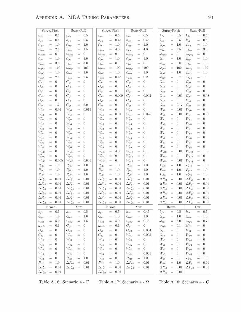
Appendix A. MDA Tuning Parameters 93
Surge/Pitch Sway/Roll
kfx = 0.5 kfy = 0.5
kωq = 0.5 kωp = 0.5
ζhpx = 1.0 ζhpy = 1.0
ωhpx = 2.5 ωhpy = 1.5
ωhpbx = 0 ωhpby = 0
ζlpx = 1.0 ζlpy = 1.0
ωlpx = 3.0 ωlpy = 3.0
ωlpbx = 100 ωlpby = 100
ζhpθ = 1.0 ζhpφ = 1.0
ωhpθ = 2.5 ωhpφ = 2.5
Gx1 = 0 Gy1 = 0
Gx2 = 0 Gy2 = 0
Gx4 = 0 Gy4 = 0
Gx5 = 0 Gy5 = 0
Gx7 = 0 Gy7 = 0
Gx8 = 1.2 Gy8 = 6.0
Wx0 = 0.01 Wy0 = 0.015
Wx1 = 0 Wy1 = 0
Wx2 = 0 Wy2 = 0
Wx3 = 0 Wy3 = 0
Wx4 = 0 Wy4 = 0
Wx5 = 0 Wy5 = 0
Wx6 = 0 Wy6 = 0
Wx7 = 0 Wy7 = 0
Wx9 = 0 Wy9 = 0
Wx10 = 0 Wy10 = 0
Wx12 = 0 Wy12 = 0
Wx13 = 0.005 Wy13 = 0.001
Px10 = 1.0 Py10 = 1.0
Px40 = 1.0 Py40 = 1.0
Px70 = 1.0 Py70 = 1.0
∆Px1 = 0.01 ∆Py1 = 0.01
∆Px2 = 0.01 ∆Py2 = 0.01
∆Px4 = 0.01 ∆Py4 = 0.01
∆Px5 = 0.01 ∆Py5 = 0.01
∆Px7 = 0.01 ∆Py7 = 0.01
∆Px8 = 0.01 ∆Py8 = 0.01
Heave Yaw
kfz = 0.5 kωr = 0.5
ζhpz = 1.0 ζhpψ = 1.0
ωhpz = 5.0 ωhpψ = 1.5
ωhpbz = 0.1 Gψ1 = 0
Gz1 = 0 Gψ2 = 0
Gz2 = 0 Wψ0 = 0
Wz0 = 0 Wψ1 = 0
Wz1 = 0 Wψ2 = 0
Wz2 = 0 Wψ3 = 0
Wz3 = 0 Wψ4 = 0
Wz4 = 0 Pψ10 = 1.0
Pz10 = 1.0 ∆Pψ1 = 0.01
∆Pz1 = 0.01 ∆Pψ2 = 0.01
∆Pz2 = 0.01
Table A.16: Scenario 4 - F
Surge/Pitch Sway/Roll
kfx = 0.5 kfy = 0.5
kωq = 0.45 kωp = 0.45
ζhpx = 1.0 ζhpy = 1.0
ωhpx = 4.0 ωhpy = 4.0
ωhpbx = 0 ωhpby = 0
ζlpx = 1.0 ζlpy = 1.0
ωlpx = 0 ωlpy = 0
ωlpbx = 100 ωlpby = 100
ζhpθ = 1.0 ζhpφ = 1.0
ωhpθ = 0.13 ωhpφ = 0.2
Gx1 = 0 Gy1 = 0
Gx2 = 0 Gy2 = 0
Gx4 = 0 Gy4 = 0
Gx5 = 0.009 Gy5 = 0.002
Gx7 = 0 Gy7 = 0
Gx8 = 0 Gy8 = 0
Wx0 = 0 Wy0 = 0
Wx1 = 0.01 Wy1 = 0.025
Wx2 = 0 Wy2 = 0
Wx3 = 0 Wy3 = 0
Wx4 = 0 Wy4 = 0
Wx5 = 0 Wy5 = 0
Wx6 = 0 Wy6 = 0
Wx7 = 0 Wy7 = 0
Wx9 = 0 Wy9 = 0
Wx10 = 4.0 Wy10 = 0.1
Wx12 = 0 Wy12 = 0
Wx13 = 0 Wy13 = 0
Px10 = 1.0 Py10 = 1.0
Px40 = 1.0 Py40 = 1.0
Px70 = 1.0 Py70 = 1.0
∆Px1 = 0.01 ∆Py1 = 0.01
∆Px2 = 0.01 ∆Py2 = 0.01
∆Px4 = 0.01 ∆Py4 = 0.01
∆Px5 = 0.01 ∆Py5 = 0.01
∆Px7 = 0.01 ∆Py7 = 0.01
∆Px8 = 0.01 ∆Py8 = 0.01
Heave Yaw
kfz = 0.5 kωr = 0.45
ζhpz = 1.0 ζhpψ = 1.0
ωhpz = 5.0 ωhpψ = 0.16
ωhpbz = 0.1 Gψ1 = 0
Gz1 = 0 Gψ2 = 0.004
Gz2 = 0 Wψ0 = 0.005
Wz0 = 0 Wψ1 = 0
Wz1 = 0 Wψ2 = 0
Wz2 = 0 Wψ3 = 0
Wz3 = 0 Wψ4 = 0.001
Wz4 = 0 Pψ10 = 1.0
Pz10 = 1.0 ∆Pψ1 = 0.01
∆Pz1 = 0.01 ∆Pψ2 = 0.01
∆Pz2 = 0.01
Table A.17: Scenario 4 - Ω
Surge/Pitch Sway/Roll
kfx = 0.5 kfy = 0.5
kωq = 0.5 kωp = 0.5
ζhpx = 1.0 ζhpy = 1.0
ωhpx = 3.5 ωhpy = 3.0
ωhpbx = 0 ωhpby = 0
ζlpx = 1.0 ζlpy = 1.0
ωlpx = 0.8 ωlpy = 1.0
ωlpbx = 100 ωlpby = 100
ζhpθ = 1.0 ζhpφ = 1.0
ωhpθ = 0.7 ωhpφ = 1.0
Gx1 = 0 Gy1 = 0
Gx2 = 0 Gy2 = 0
Gx4 = 0 Gy4 = 0
Gx5 = 0.03 Gy5 = 0.08
Gx7 = 0 Gy7 = 0
Gx8 = 0.17 Gy8 = 0
Wx0 = 0.01 Wy0 = 0
Wx1 = 0.01 Wy1 = 0.01
Wx2 = 0 Wy2 = 0
Wx3 = 0 Wy3 = 0
Wx4 = 0 Wy4 = 0
Wx5 = 0 Wy5 = 0
Wx6 = 0 Wy6 = 0
Wx7 = 0 Wy7 = 0
Wx9 = 0 Wy9 = 0
Wx10 = 0.01 Wy10 = 1.0
Wx12 = 0 Wy12 = 0
Wx13 = 0.01 Wy13 = 0
Px10 = 1.0 Py10 = 1.0
Px40 = 1.0 Py40 = 1.0
Px70 = 1.0 Py70 = 1.0
∆Px1 = 0.01 ∆Py1 = 0.01
∆Px2 = 0.01 ∆Py2 = 0.01
∆Px4 = 0.01 ∆Py4 = 0.01
∆Px5 = 0.01 ∆Py5 = 0.01
∆Px7 = 0.01 ∆Py7 = 0.01
∆Px8 = 0.01 ∆Py8 = 0.01
Heave Yaw
kfz = 0.5 kωr = 0.5
ζhpz = 1.0 ζhpψ = 1.0
ωhpz = 5.0 ωhpψ = 0.7
ωhpbz = 0.1 Gψ1 = 0
Gz1 = 0 Gψ2 = 0
Gz2 = 0 Wψ0 = 0
Wz0 = 0 Wψ1 = 0
Wz1 = 0 Wψ2 = 0
Wz2 = 0 Wψ3 = 0
Wz3 = 0 Wψ4 = 0
Wz4 = 0 Pψ10 = 1.0
Pz10 = 1.0 ∆Pψ1 = 0.01
∆Pz1 = 0.01 ∆Pψ2 = 0.01
∆Pz2 = 0.01
Table A.18: Scenario 4 - C
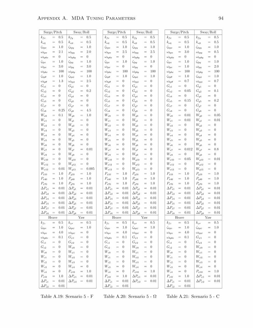
Appendix A. MDA Tuning Parameters 94
Surge/Pitch Sway/Roll
kfx = 0.5 kfy = 0.5
kωq = 0.5 kωp = 0.5
ζhpx = 1.0 ζhpy = 1.0
ωhpx = 2.1 ωhpy = 2.0
ωhpbx = 0 ωhpby = 0
ζlpx = 1.0 ζlpy = 1.0
ωlpx = 3.0 ωlpy = 3.0
ωlpbx = 100 ωlpby = 100
ζhpθ = 1.0 ζhpφ = 1.0
ωhpθ = 1.3 ωhpφ = 2.5
Gx1 = 0 Gy1 = 0
Gx2 = 0 Gy2 = 0.2
Gx4 = 0 Gy4 = 0
Gx5 = 0 Gy5 = 0
Gx7 = 0 Gy7 = 0
Gx8 = 0.25 Gy8 = 4.5
Wx0 = 0.1 Wy0 = 1.0
Wx1 = 0 Wy1 = 0
Wx2 = 0 Wy2 = 0
Wx3 = 0 Wy3 = 0
Wx4 = 0 Wy4 = 0
Wx5 = 0 Wy5 = 0
Wx6 = 0 Wy6 = 0
Wx7 = 0 Wy7 = 0.01
Wx9 = 0 Wy9 = 0
Wx10 = 0 Wy10 = 0
Wx12 = 0 Wy12 = 0
Wx13 = 0.01 Wy13 = 0.005
Px10 = 1.0 Py10 = 1.0
Px40 = 1.0 Py40 = 1.0
Px70 = 1.0 Py70 = 1.0
∆Px1 = 0.01 ∆Py1 = 0.01
∆Px2 = 0.01 ∆Py2 = 0.01
∆Px4 = 0.01 ∆Py4 = 0.01
∆Px5 = 0.01 ∆Py5 = 0.01
∆Px7 = 0.01 ∆Py7 = 0.01
∆Px8 = 0.01 ∆Py8 = 0.01
Heave Yaw
kfz = 0.5 kωr = 0.5
ζhpz = 1.0 ζhpψ = 1.0
ωhpz = 4.0 ωhpψ = 0
ωhpbz = 0.1 Gψ1 = 0
Gz1 = 0 Gψ2 = 0
Gz2 = 0 Wψ0 = 0
Wz0 = 0 Wψ1 = 0
Wz1 = 0 Wψ2 = 0
Wz2 = 0 Wψ3 = 0
Wz3 = 0 Wψ4 = 0
Wz4 = 0 Pψ10 = 1.0
Pz10 = 1.0 ∆Pψ1 = 0.01
∆Pz1 = 0.01 ∆Pψ2 = 0.01
∆Pz2 = 0.01
Table A.19: Scenario 5 - F
Surge/Pitch Sway/Roll
kfx = 0.5 kfy = 0.5
kωq = 0.5 kωp = 0.5
ζhpx = 1.0 ζhpy = 1.0
ωhpx = 2.5 ωhpy = 2.5
ωhpbx = 0 ωhpby = 0
ζlpx = 1.0 ζlpy = 1.0
ωlpx = 0 ωlpy = 0
ωlpbx = 100 ωlpby = 100
ζhpθ = 1.0 ζhpφ = 1.0
ωhpθ = 0 ωhpφ = 0
Gx1 = 0 Gy1 = 0
Gx2 = 0 Gy2 = 0
Gx4 = 0 Gy4 = 0
Gx5 = 0 Gy5 = 0
Gx7 = 0 Gy7 = 0
Gx8 = 0 Gy8 = 0
Wx0 = 0 Wy0 = 0
Wx1 = 0 Wy1 = 0
Wx2 = 0 Wy2 = 0
Wx3 = 0 Wy3 = 0
Wx4 = 0 Wy4 = 0
Wx5 = 0 Wy5 = 0
Wx6 = 0 Wy6 = 0
Wx7 = 0 Wy7 = 0
Wx9 = 0 Wy9 = 0
Wx10 = 0 Wy10 = 0
Wx12 = 0 Wy12 = 0
Wx13 = 0 Wy13 = 0
Px10 = 1.0 Py10 = 1.0
Px40 = 1.0 Py40 = 1.0
Px70 = 1.0 Py70 = 1.0
∆Px1 = 0.01 ∆Py1 = 0.01
∆Px2 = 0.01 ∆Py2 = 0.01
∆Px4 = 0.01 ∆Py4 = 0.01
∆Px5 = 0.01 ∆Py5 = 0.01
∆Px7 = 0.01 ∆Py7 = 0.01
∆Px8 = 0.01 ∆Py8 = 0.01
Heave Yaw
kfz = 0.5 kωr = 0.5
ζhpz = 1.0 ζhpψ = 1.0
ωhpz = 4.0 ωhpψ = 0
ωhpbz = 0.1 Gψ1 = 0
Gz1 = 0 Gψ2 = 0
Gz2 = 0 Wψ0 = 0
Wz0 = 0 Wψ1 = 0
Wz1 = 0 Wψ2 = 0
Wz2 = 0 Wψ3 = 0
Wz3 = 0 Wψ4 = 0
Wz4 = 0 Pψ10 = 1.0
Pz10 = 1.0 ∆Pψ1 = 0.01
∆Pz1 = 0.01 ∆Pψ2 = 0.01
∆Pz2 = 0.01
Table A.20: Scenario 5 - Ω
Surge/Pitch Sway/Roll
kfx = 0.5 kfy = 0.5
kωq = 0.5 kωp = 0.5
ζhpx = 1.0 ζhpy = 1.0
ωhpx = 3.0 ωhpy = 0.5
ωhpbx = 0 ωhpby = 0
ζlpx = 1.0 ζlpy = 1.0
ωlpx = 1.0 ωlpy = 2.0
ωlpbx = 100 ωlpby = 100
ζhpθ = 1.0 ζhpφ = 1.0
ωhpθ = 0.7 ωhpφ = 0.7
Gx1 = 0 Gy1 = 0
Gx2 = 0.05 Gy2 = 0.1
Gx4 = 0 Gy4 = 0
Gx5 = 0.15 Gy5 = 0.2
Gx7 = 0 Gy7 = 0
Gx8 = 0 Gy8 = 0
Wx0 = 0.01 Wy0 = 0.05
Wx1 = 0.01 Wy1 = 0.01
Wx2 = 0 Wy2 = 0
Wx3 = 0 Wy3 = 0
Wx4 = 0 Wy4 = 0
Wx5 = 0 Wy5 = 0
Wx6 = 0 Wy6 = 0
Wx7 = 0.012 Wy7 = 0.8
Wx9 = 0 Wy9 = 0
Wx10 = 0.05 Wy10 = 0.01
Wx12 = 0 Wy12 = 0
Wx13 = 0 Wy13 = 0
Px10 = 1.0 Py10 = 1.0
Px40 = 1.0 Py40 = 1.0
Px70 = 1.0 Py70 = 1.0
∆Px1 = 0.01 ∆Py1 = 0.01
∆Px2 = 0.01 ∆Py2 = 0.01
∆Px4 = 0.01 ∆Py4 = 0.01
∆Px5 = 0.01 ∆Py5 = 0.01
∆Px7 = 0.01 ∆Py7 = 0.01
∆Px8 = 0.01 ∆Py8 = 0.01
Heave Yaw
kfz = 0.5 kωr = 0.5
ζhpz = 1.0 ζhpψ = 1.0
ωhpz = 4.0 ωhpψ = 0
ωhpbz = 0.1 Gψ1 = 0
Gz1 = 0 Gψ2 = 0
Gz2 = 0 Wψ0 = 0
Wz0 = 0 Wψ1 = 0
Wz1 = 0 Wψ2 = 0
Wz2 = 0 Wψ3 = 0
Wz3 = 0 Wψ4 = 0
Wz4 = 0 Pψ10 = 1.0
Pz10 = 1.0 ∆Pψ1 = 0.01
∆Pz1 = 0.01 ∆Pψ2 = 0.01
∆Pz2 = 0.01
Table A.21: Scenario 5 - C
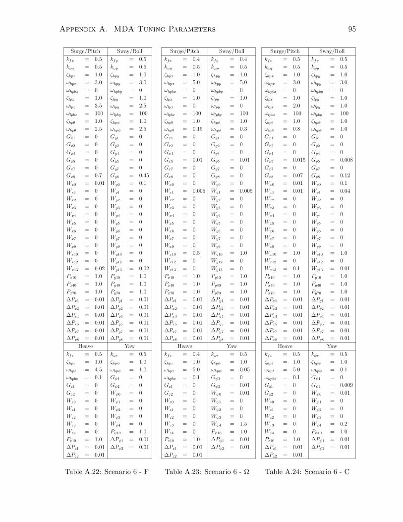
Appendix A. MDA Tuning Parameters 95
Surge/Pitch Sway/Roll
kfx = 0.5 kfy = 0.5
kωq = 0.5 kωp = 0.5
ζhpx = 1.0 ζhpy = 1.0
ωhpx = 3.0 ωhpy = 3.0
ωhpbx = 0 ωhpby = 0
ζlpx = 1.0 ζlpy = 1.0
ωlpx = 3.5 ωlpy = 2.5
ωlpbx = 100 ωlpby = 100
ζhpθ = 1.0 ζhpφ = 1.0
ωhpθ = 2.5 ωhpφ = 2.5
Gx1 = 0 Gy1 = 0
Gx2 = 0 Gy2 = 0
Gx4 = 0 Gy4 = 0
Gx5 = 0 Gy5 = 0
Gx7 = 0 Gy7 = 0
Gx8 = 0.7 Gy8 = 0.45
Wx0 = 0.01 Wy0 = 0.1
Wx1 = 0 Wy1 = 0
Wx2 = 0 Wy2 = 0
Wx3 = 0 Wy3 = 0
Wx4 = 0 Wy4 = 0
Wx5 = 0 Wy5 = 0
Wx6 = 0 Wy6 = 0
Wx7 = 0 Wy7 = 0
Wx9 = 0 Wy9 = 0
Wx10 = 0 Wy10 = 0
Wx12 = 0 Wy12 = 0
Wx13 = 0.02 Wy13 = 0.02
Px10 = 1.0 Py10 = 1.0
Px40 = 1.0 Py40 = 1.0
Px70 = 1.0 Py70 = 1.0
∆Px1 = 0.01 ∆Py1 = 0.01
∆Px2 = 0.01 ∆Py2 = 0.01
∆Px4 = 0.01 ∆Py4 = 0.01
∆Px5 = 0.01 ∆Py5 = 0.01
∆Px7 = 0.01 ∆Py7 = 0.01
∆Px8 = 0.01 ∆Py8 = 0.01
Heave Yaw
kfz = 0.5 kωr = 0.5
ζhpz = 1.0 ζhpψ = 1.0
ωhpz = 4.5 ωhpψ = 1.0
ωhpbz = 0.1 Gψ1 = 0
Gz1 = 0 Gψ2 = 0
Gz2 = 0 Wψ0 = 0
Wz0 = 0 Wψ1 = 0
Wz1 = 0 Wψ2 = 0
Wz2 = 0 Wψ3 = 0
Wz3 = 0 Wψ4 = 0
Wz4 = 0 Pψ10 = 1.0
Pz10 = 1.0 ∆Pψ1 = 0.01
∆Pz1 = 0.01 ∆Pψ2 = 0.01
∆Pz2 = 0.01
Table A.22: Scenario 6 - F
Surge/Pitch Sway/Roll
kfx = 0.4 kfy = 0.4
kωq = 0.5 kωp = 0.5
ζhpx = 1.0 ζhpy = 1.0
ωhpx = 5.0 ωhpy = 5.0
ωhpbx = 0 ωhpby = 0
ζlpx = 1.0 ζlpy = 1.0
ωlpx = 0 ωlpy = 0
ωlpbx = 100 ωlpby = 100
ζhpθ = 1.0 ζhpφ = 1.0
ωhpθ = 0.15 ωhpφ = 0.3
Gx1 = 0 Gy1 = 0
Gx2 = 0 Gy2 = 0
Gx4 = 0 Gy4 = 0
Gx5 = 0.01 Gy5 = 0.01
Gx7 = 0 Gy7 = 0
Gx8 = 0 Gy8 = 0
Wx0 = 0 Wy0 = 0
Wx1 = 0.005 Wy1 = 0.005
Wx2 = 0 Wy2 = 0
Wx3 = 0 Wy3 = 0
Wx4 = 0 Wy4 = 0
Wx5 = 0 Wy5 = 0
Wx6 = 0 Wy6 = 0
Wx7 = 0 Wy7 = 0
Wx9 = 0 Wy9 = 0
Wx10 = 0.5 Wy10 = 1.0
Wx12 = 0 Wy12 = 0
Wx13 = 0 Wy13 = 0
Px10 = 1.0 Py10 = 1.0
Px40 = 1.0 Py40 = 1.0
Px70 = 1.0 Py70 = 1.0
∆Px1 = 0.01 ∆Py1 = 0.01
∆Px2 = 0.01 ∆Py2 = 0.01
∆Px4 = 0.01 ∆Py4 = 0.01
∆Px5 = 0.01 ∆Py5 = 0.01
∆Px7 = 0.01 ∆Py7 = 0.01
∆Px8 = 0.01 ∆Py8 = 0.01
Heave Yaw
kfz = 0.4 kωr = 0.5
ζhpz = 1.0 ζhpψ = 1.0
ωhpz = 5.0 ωhpψ = 0.05
ωhpbz = 0.1 Gψ1 = 0
Gz1 = 0 Gψ2 = 0.01
Gz2 = 0 Wψ0 = 0.01
Wz0 = 0 Wψ1 = 0
Wz1 = 0 Wψ2 = 0
Wz2 = 0 Wψ3 = 0
Wz3 = 0 Wψ4 = 1.5
Wz4 = 0 Pψ10 = 1.0
Pz10 = 1.0 ∆Pψ1 = 0.01
∆Pz1 = 0.01 ∆Pψ2 = 0.01
∆Pz2 = 0.01
Table A.23: Scenario 6 - Ω
Surge/Pitch Sway/Roll
kfx = 0.5 kfy = 0.5
kωq = 0.5 kωp = 0.5
ζhpx = 1.0 ζhpy = 1.0
ωhpx = 3.0 ωhpy = 3.0
ωhpbx = 0 ωhpby = 0
ζlpx = 1.0 ζlpy = 1.0
ωlpx = 2.0 ωlpy = 1.0
ωlpbx = 100 ωlpby = 100
ζhpθ = 1.0 ζhpφ = 1.0
ωhpθ = 0.8 ωhpφ = 1.0
Gx1 = 0 Gy1 = 0
Gx2 = 0 Gy2 = 0
Gx4 = 0 Gy4 = 0
Gx5 = 0.015 Gy5 = 0.008
Gx7 = 0 Gy7 = 0
Gx8 = 0.07 Gy8 = 0.12
Wx0 = 0.01 Wy0 = 0.1
Wx1 = 0.01 Wy1 = 0.04
Wx2 = 0 Wy2 = 0
Wx3 = 0 Wy3 = 0
Wx4 = 0 Wy4 = 0
Wx5 = 0 Wy5 = 0
Wx6 = 0 Wy6 = 0
Wx7 = 0 Wy7 = 0
Wx9 = 0 Wy9 = 0
Wx10 = 1.0 Wy10 = 1.0
Wx12 = 0 Wy12 = 0
Wx13 = 0.1 Wy13 = 0.01
Px10 = 1.0 Py10 = 1.0
Px40 = 1.0 Py40 = 1.0
Px70 = 1.0 Py70 = 1.0
∆Px1 = 0.01 ∆Py1 = 0.01
∆Px2 = 0.01 ∆Py2 = 0.01
∆Px4 = 0.01 ∆Py4 = 0.01
∆Px5 = 0.01 ∆Py5 = 0.01
∆Px7 = 0.01 ∆Py7 = 0.01
∆Px8 = 0.01 ∆Py8 = 0.01
Heave Yaw
kfz = 0.5 kωr = 0.5
ζhpz = 1.0 ζhpψ = 1.0
ωhpz = 5.0 ωhpψ = 0.1
ωhpbz = 0.1 Gψ1 = 0
Gz1 = 0 Gψ2 = 0.009
Gz2 = 0 Wψ0 = 0.01
Wz0 = 0 Wψ1 = 0
Wz1 = 0 Wψ2 = 0
Wz2 = 0 Wψ3 = 0
Wz3 = 0 Wψ4 = 0.2
Wz4 = 0 Pψ10 = 1.0
Pz10 = 1.0 ∆Pψ1 = 0.01
∆Pz1 = 0.01 ∆Pψ2 = 0.01
∆Pz2 = 0.01
Table A.24: Scenario 6 - C
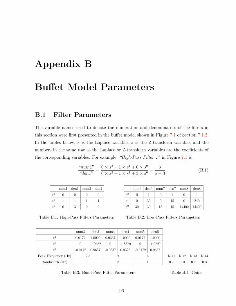
Appendix B
Buffet Model Parameters
B.1 Filter Parameters
The variable names used to denote the numerators and denominators of the filters in
this section were first presented in the buffet model shown in Figure 7.1 of Section 7.1.2.
In the tables below, s is the Laplace variable, z is the Z-transform variable, and the
numbers in the same row as the Laplace or Z-transform variables are the coefficients of
the corresponding variables. For example, “High-Pass Filter 1” in Figure 7.1 is
“num1”
“den1”=
0× s2 + 1× s1 + 0× s0
0× s2 + 1× s1 + 3× s0=
s
s+ 3(B.1)
num1 den1 num2 den2
s2 0 0 0 0
s1 1 1 1 1
s0 0 3 0 9
Table B.1: High-Pass Filters Parameters
num6 den6 num7 den7 num8 den8
s2 0 1 0 1 0 1
s1 0 30 0 15 0 240
s0 30 30 15 15 14400 14400
Table B.2: Low-Pass Filters Parameters
num3 den3 num4 den4 num5 den5
z2 0.0172 1.0000 0.0337 1.0000 0.0172 1.0000
z1 0 -1.9582 0 -1.8379 0 -1.9227
z0 -0.0172 0.9657 -0.0337 0.9325 -0.0172 0.9657
Peak Frequency (Hz) 2.5 9 6
Bandwidth (Hz) 1 2 1
Table B.3: Band-Pass Filter Parameters
K r1 K r2 K r3 K r4
0.7 1.0 0.7 0.3
Table B.4: Gains
96
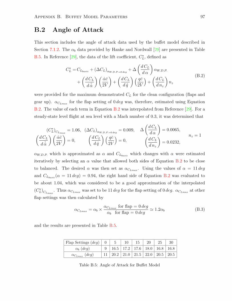
Appendix B. Buffet Model Parameters 97
B.2 Angle of Attack
This section includes the angle of attack data used by the buffet model described in
Section 7.1.2. The αb data provided by Hanke and Nordwall [29] are presented in Table
B.5. In Reference [29], the data of the lift coefficient, C∗L, defined as
C∗L =CLbasic + (∆CL)αW.D.P.=0 deg+ ∆
(dCLdα
)αW.D.P.
+
(dCL
d ˆα
)(αc
2V
)+
(dCLd q
)( qc2V
)+
(dCLd nz
)nz
(B.2)
were provided for the maximum demonstrated CL for the clean configuration (flaps and
gear up). αCLmax for the flap setting of 0 deg was, therefore, estimated using Equation
B.2. The value of each term in Equation B.2 was interpolated from Reference [29]. For a
steady-state level flight at sea level with a Mach number of 0.3, it was determined that
(C∗L)CLmax = 1.06,(dCL
d ˆα
)(αc
2V
)= 0,
(∆CL)αW.D.P.=0 deg= 0.009,(
dCLd q
)( qc2V
)= 0,
∆
(dCLdα
)= 0.0065,(
dCLd nz
)= 0.0232,
nz = 1
αW.D.P. which is approximated as α and CLbasic which changes with α were estimated
iteratively by selecting an α value that allowed both sides of Equation B.2 to be close
to balanced. The desired α was then set as αCLmax . Using the values of α = 11 deg
and CLbasic(α = 11 deg) = 0.94, the right hand side of Equation B.2 was evaluated to
be about 1.04, which was considered to be a good approximation of the interpolated
(C∗L)CLmax . Thus αCLmax was set to be 11 deg for the flap setting of 0 deg. αCLmax at other
flap settings was then calculated by
αCLmax = αb ×αCLmax for flap = 0 deg
αb for flap = 0 deg' 1.2αb (B.3)
and the results are presented in Table B.5.
Flap Settings (deg) 0 5 10 15 20 25 30
αb (deg) 9 16.5 17.2 17.6 18.0 16.8 16.8
αCLmax (deg) 11 20.2 21.0 21.5 22.0 20.5 20.5
Table B.5: Angle of Attack for Buffet Model
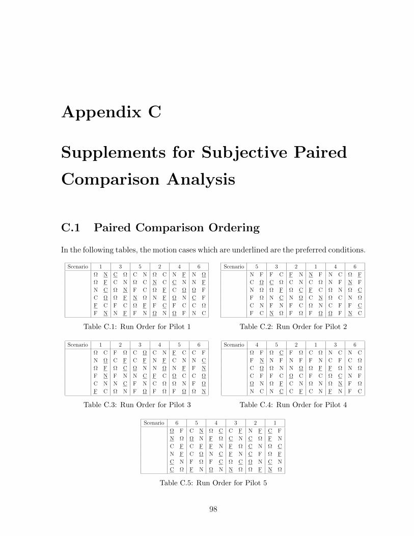
Appendix C
Supplements for Subjective Paired
Comparison Analysis
C.1 Paired Comparison Ordering
In the following tables, the motion cases which are underlined are the preferred conditions.
Scenario 1 3 5 2 4 6
Ω N C Ω C N Ω C N F N Ω
Ω F C N Ω C N C C N N F
N C Ω N F C Ω F C Ω Ω F
C Ω Ω F N Ω N F Ω N C F
F C F C Ω F F C F C C Ω
F N N F F N Ω N Ω F N C
Table C.1: Run Order for Pilot 1
Scenario 5 3 2 1 4 6
N F F C F N N F N C Ω F
C Ω C Ω C N C Ω N F N F
N Ω Ω F Ω C F C Ω N Ω C
F Ω N C N Ω C N Ω C N Ω
C N F N F C Ω N C F F C
F C N Ω F Ω F Ω Ω F N C
Table C.2: Run Order for Pilot 2
Scenario 1 2 3 4 5 6
Ω C F Ω C Ω C N F C C F
N Ω C F C F N F C N N C
Ω F Ω C Ω N N Ω N F F N
F N F N N C F C Ω C C Ω
C N N C F N C Ω Ω N F Ω
F C Ω N F Ω F Ω F Ω Ω N
Table C.3: Run Order for Pilot 3
Scenario 4 5 2 1 3 6
Ω F Ω C F Ω C Ω N C N C
F N N F N F F N C F C Ω
C Ω Ω N N Ω Ω F F Ω N Ω
C F F C Ω C F C Ω C N F
Ω N Ω F C N Ω N Ω N F Ω
N C N C C F C N F N F C
Table C.4: Run Order for Pilot 4
Scenario 6 5 4 3 2 1
Ω F C N Ω C C F N F C F
N Ω Ω N F Ω C N C Ω F N
C F C F F N F Ω C N Ω C
N F C Ω N C F N C F Ω F
C N F Ω F C Ω C Ω N C N
C Ω F N Ω N N Ω Ω F N Ω
Table C.5: Run Order for Pilot 5
98
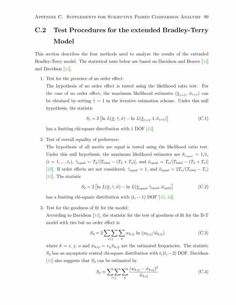
Appendix C. Supplements for Subjective Paired Comparison Analysis 99
C.2 Test Procedures for the extended Bradley-Terry
Model
This section describes the four methods used to analyze the results of the extended
Bradley-Terry model. The statistical tests below are based on Davidson and Beaver [43]
and Davidson [44].
1. Test for the presence of an order effect:
The hypothesis of no order effect is tested using the likelihood ratio test. For
the case of no order effect, the maximum likelihood estimates (πγ=1, νγ=1) can
be obtained by setting γ = 1 in the iterative estimation scheme. Under this null
hypothesis, the statistic
S1 = 2[ln L(π, γ, ν)− ln L(πγ=1, 1, νγ=1)
](C.1)
has a limiting chi-square distribution with 1 DOF [43].
2. Test of overall equality of preference:
The hypothesis of all merits are equal is tested using the likelihood ratio test.
Under this null hypothesis, the maximum likelihood estimates are πiequal = 1/tc
(i = 1, ... , tc), γequal = T2/[Ttotal − (T2 + To)], and νequal = To/[Ttotal − (T2 + To)]
[43]. If order effects are not considered, γequal = 1, and νequal = 2To/(Ttotal − To)[44]. The statistic
S2 = 2[ln L(π, γ, ν)− ln L(πequal, γequal, νequal
](C.2)
has a limiting chi-square distribution with (tc − 1) DOF [43, 44].
3. Test for the goodness of fit for the model:
According to Davidson [44], the statistic for the test of goodness of fit for the B-T
model with ties but no order effect is
S3 = 2∑∑
i<j
∑k
wk,ij ln (wk,ij/wk,ij) (C.3)
where k = i, j, o and wk,ij = rijπk,ij are the estimated frequencies. The statistic
S3 has an asymptotic central chi-square distribution with tc(tc−2) DOF. Davidson
[44] also suggests that S3 can be estimated by
S3 '∑∑
i<j
∑k
(wk,ij − wk,ij)2
wk,ij(C.4)
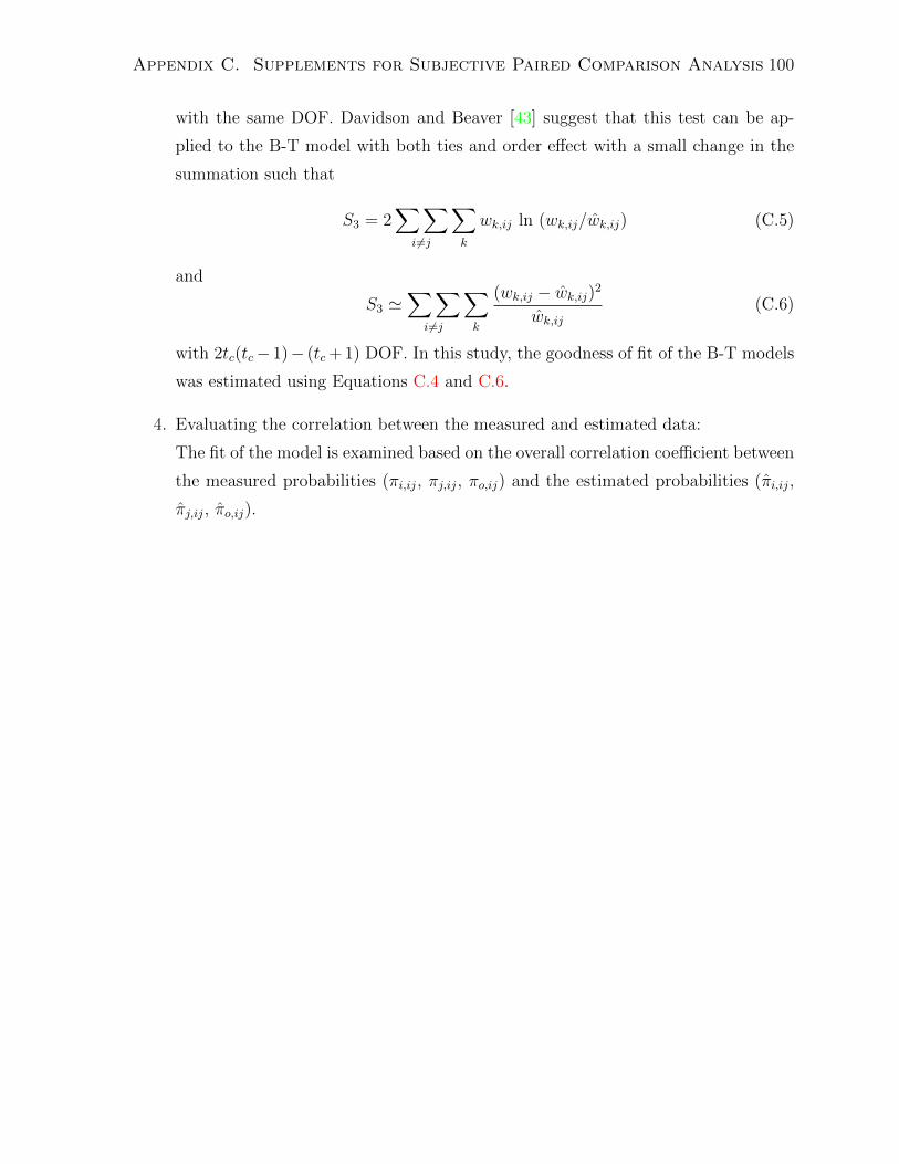
Appendix C. Supplements for Subjective Paired Comparison Analysis 100
with the same DOF. Davidson and Beaver [43] suggest that this test can be ap-
plied to the B-T model with both ties and order effect with a small change in the
summation such that
S3 = 2∑∑
i 6=j
∑k
wk,ij ln (wk,ij/wk,ij) (C.5)
and
S3 '∑∑
i 6=j
∑k
(wk,ij − wk,ij)2
wk,ij(C.6)
with 2tc(tc− 1)− (tc + 1) DOF. In this study, the goodness of fit of the B-T models
was estimated using Equations C.4 and C.6.
4. Evaluating the correlation between the measured and estimated data:
The fit of the model is examined based on the overall correlation coefficient between
the measured probabilities (πi,ij, πj,ij, πo,ij) and the estimated probabilities (πi,ij,
πj,ij, πo,ij).