Computer Science Honours

Literature Review

An Investigation of Digital Mixing andPanning Algorithms

Jessica Kent

Department of Computer Science, Rhodes University

Supervisor:Richard Foss

Consultant:Corinne Cooper

May 30, 2014

Abstract

The difference between the summing quality of analogue and digi-tal audio is widely debated. Possible causes for this such as samplingrates, frequency response in human hearing and panning laws are con-sidered. A study of how three open source Digital Audio Workstations(DAWs) define and implement gain, panning and summing of individ-ual samples is then discussed. It was found that although samples weresummed similarly, the execution of panning was distinct for each DAW.Previous testing of DAWs and alternate methods for summing sampleswere also reviewed.

1

Contents

1 Introduction 3

2 Analogue vs Digital 32.1 Definitions and Concepts in Audio Recording . . . . . . . . . 32.2 Sound Waves and Sample Rates . . . . . . . . . . . . . . . . . 52.3 Fletcher-Munson curves . . . . . . . . . . . . . . . . . . . . . 62.4 Panning Laws . . . . . . . . . . . . . . . . . . . . . . . . . . . 72.5 Analogue Equipment . . . . . . . . . . . . . . . . . . . . . . . 8

3 Mixing Algorithms 83.1 Representation of Gain . . . . . . . . . . . . . . . . . . . . . . 93.2 Panning Laws . . . . . . . . . . . . . . . . . . . . . . . . . . . 93.3 Summing of Samples . . . . . . . . . . . . . . . . . . . . . . . 103.4 Alternative Summing Methods . . . . . . . . . . . . . . . . . . 11

4 Testing 124.1 Objective Testing Methods . . . . . . . . . . . . . . . . . . . . 144.2 Subjective Testing Methods . . . . . . . . . . . . . . . . . . . 144.3 Previous Testing . . . . . . . . . . . . . . . . . . . . . . . . . 144.4 Timing . . . . . . . . . . . . . . . . . . . . . . . . . . . . . . . 15

5 Summary 15

References 17

A Audacity Code 19

B Ardour Code 20

C Rosegarden Code 22

2

1 Introduction

When audio files are added together, or summed, in a Digital Audio Work-station to create a final stereo track, the sound quality is missing the warmthand depth that the track would have if it had been summed using an ana-logue console. The hypothesis for this thesis is that a mechanism to providethe characteristics of an analogue mixer can be found and implemented in adigital mix.

2 Analogue vs Digital

In the sound engineering community there is debate about the sound qualityof an audio mix that has been digitally summed instead of summed using ananalogue mixing console. For the purpose of this paper, the terms “summing”and “mixing” will be used interchangeably and an “analogue” sample willrefer to audio that has been summed in an analogue console, even if it playedfrom a digital system. Some professionals say that a digital mix is lackingthe “undeniable depth, width, punch and realism” (Farmelo, 2011, p. 1) of ananalogue mix. However, as Leonard et al. (2012, p. 1) states, there is not much“quantifiable evidence to support these claims” yet. And although others,like Cochrane (2012), point out that summing with a DAW or analogue consolewon’t necessarily improve the quality of a song if it has not been correctlymixed (artistically speaking), it is generally accepted that the limitations ofanalogue equipment might account for the difference in the perceived characterof the mix (Cooper, 2004). For sound engineers who have been recording andmixing for the past 20 years, this unexplained variation of sound is a sourceof frustration, and summing boxes, like the Crane Song Egret or Rupert NeveDesign 5059 (Sound on Sound, 2012), are being sold for the sole purpose ofcreating an analogue mix.

2.1 Definitions and Concepts in Audio Recording

In order to begin comparing digital and analogue mixing methods, some back-ground information about audio recording is needed. Audio was first recordedusing analogue equipment, usually onto magnetized tape. A recording device,typically a microphone, would record and convert fluctuations in air pressureto a measurable electronic signal. These varying electrical signals would thenbe recorded onto tape (Watkinson, 2001). As technology has advanced, digitalequipment has been created to record, edit and mix audio signals. However,

3

microphones still capture analogue signals, so some kind of conversion needs totake place for audio to be processed using a Digital Audio Workstation (DAW).This has triggered many discussions about the quality variations between ana-logue and digital equipment and even among the “perceivable difference insound quality between different DAWs” themselves, as stated by Leonard et al.(2012, p. 1).

To convert the recorded voltages to a digital audio signal, measurements ofthe voltages, called samples, are taken at fixed time intervals. This pulse codemodulation (PCM) method is generally accepted as the standard system usedin the conversion process (Lipshitz & Vanderkooy, 2004, p. 200). To make surenone of the original signal is lost, samples need to be taken at very high rates of44.1kHz, 48kHz, 96kHz and 192kHz. An example of a wave being sampled attwo different rates, the first one much lower than the other, is shown in Fig. 1.The rate of 44.1kHz was chosen to be used on digital compact discs (CDs) fornumerous reasons - one of which is that it is more than twice the rate of thehighest frequency humans can hear (Watkinson, 2001, pp. 207–209). This is aresult of the Nyquist Theorem, which states that at least two sample pointsare needed to recreate a wave of a specific frequency (Lipshitz & Vanderkooy,2004, p. 201). These samples are then stored numerically and can be used torecreate and modify the recorded sound wave (Watkinson, 2001).

Figure 1: Sound wave sampled at two different rates (Rabiner, 1982, p. 80)

The amplitude or level of an audio wave is measured in deciBels - a log-arithmic scale named after Alexander Graham Bell (Watkinson, 2001, p. 66).

4

The standard calculation used to convert a ratio value (generally between 0and 1) to it’s deciBel equivalent is given in Equation 1 (Watkinson, 2001,p. 66).

deciBels = 20 · log10(amplitude ratio) (1)

Just as the maximum frequency that can be stored is determined by thechoice of sample rate, the bit depth limits the amount of signal that can bestored by a digital system. When an input signal is too loud and the amplitudeof the sound wave is too big for a digital system to store, the wave ‘clips’causing the sound to distort (Cornell, 2009). The industry standard bit depthfor CDs is 16-bit although audio is usually recorded and processed at 24-bit or32-bit and converted to 16-bit after being mixed and mastered (Izhaki, 2008,p. 51).

2.2 Sound Waves and Sample Rates

A sound wave being produced by a musical instrument is typically a complexwave, made up of the fundamental frequency and higher harmonics (or over-tones) that are a positive multiple of the fundamental frequency. In the 1800s,Joseph Fourier discovered that any existing sound wave can be representedmathematically as a sum of “simple harmonic terms” (Kinsler, 1962, p. 15),which are usually sine waves. This means that the sound wave in Fig. 2 canbe expressed as the sum of two sine waves.

Figure 2: Sound wave comprised of two sine waves (Agilent Technologies, 2000,p. 7)

In conventional DAWs audio is recorded and summed at a sampling rateof either 44.1kHz or 48kHz. According to the Nyquist Theorem, frequenciesabove half the sampling rate (i.e. 22.05kHz or 24kHz respectively) are notrecorded because there are not enough sample points to recreate them. How-ever, as Izhaki (2008, pp. 456–457) points out, if a complex wave or any dis-tortion is recorded at 48kHz, the harmonics of the wave above 24kHz will not

5

be recorded. This is not a problem on an analogue console. Although humanscannot hear sound waves higher than 20kHz (Watkinson, 2001, pp. 45-46), theyare still recorded by the analogue console. When multiple audio tracks, oneor more of which contains sound waves above 24kHz, are digitized and thensummed together, it is theoretically possible that this high frequency wave willaffect sounds waves below 20kHz. This would affect what humans can hearand could possibly be the difference heard when summing audio digitally.

However, Watkinson (2001, pp. 729-730) emphatically says that althoughdemonstrations may have shown that higher sampling rates sound better, theexperiments were not designed or carried out correctly. He also states thatwhile converters sampling at 96kHz have been proven to sound better, “thisdoes not prove that 96kHz is necessary” (Watkinson, 2001, p. 730) because abetter designed converter sampling at a lower rate could produce the sameresults.

2.3 Fletcher-Munson curves

Not only are human ears limited to the frequencies they can hear, but theyperceive some frequencies to be louder or softer than others. A set of experi-ments performed by Harvey Fletcher and W.A. Munson in 1933 (Izhaki, 2008,p. 12) resulted in the Feltcher-Munson curves (as shown in Fig. 3). Thesecurves show that in order to hear a bass frequency under 100Hz as loud asa mid-range frequency of, say a 1kHz wave, the level of the audio needs tobe higher. In other words, bass frequencies are not heard clearly in softeraudio but our ears are very receptive to frequencies between about 2kHz and5kHz (Watkinson, 2001, p. 45).

Figure 3: Fletcher-Munson curves (Watkinson, 2001, p. 46)

6

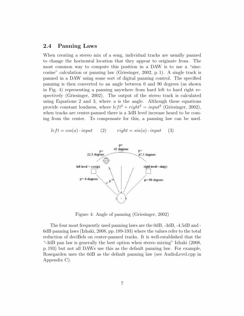
2.4 Panning Laws

When creating a stereo mix of a song, individual tracks are usually pannedto change the horizontal location that they appear to originate from. Themost common way to compute this position in a DAW is to use a “sine-cosine” calculation or panning law (Griesinger, 2002, p. 1). A single track ispanned in a DAW using some sort of digital panning control. The specifiedpanning is then converted to an angle between 0 and 90 degrees (as shownin Fig. 4) representing a panning anywhere from hard left to hard right re-spectively (Griesinger, 2002). The output of the stereo track is calculatedusing Equations 2 and 3, where a is the angle. Although these equationsprovide constant loudness, where left2 + right2 = input2 (Griesinger, 2002),when tracks are center-panned there is a 3dB level increase heard to be com-ing from the center. To compensate for this, a panning law can be used.

left = cos(a) · input (2) right = sin(a) · input (3)

Figure 4: Angle of panning (Griesinger, 2002)

The four most frequently used panning laws are the 0dB, -3dB, -4.5dB and -6dB panning laws (Izhaki, 2008, pp. 189-193) where the values refer to the totalreduction of deciBels on center-panned tracks. It is well-established that the“-3dB pan law is generally the best option when stereo mixing” Izhaki (2008,p. 193) but not all DAWs use this as the default panning law. For example,Rosegarden uses the 0dB as the default panning law (see AudioLevel.cpp inAppendix C).

7

2.5 Analogue Equipment

When examining various digital summing algorithms it is useful to investi-gate how an analogue mixer combines signals to produce a summed output.An example of a summing amplifier circuit is shown in Fig. 5 where threeinput signals (V1, V2 and V3) are added together to produce an output volt-age (−Vout). When the input impedances (−RIN) are the same, the outputcan be calculated using Equation 4. This means that the output voltage isproportional to the sum of the input voltages (Storr, 2014).

−Vout =RF

RIn

(V1 + V2 + V3) (4)

Figure 5: Summing Amplifier Circuit (Storr, 2014)

3 Mixing Algorithms

Since a song typically consists of multiple tracks, a DAW needs to be able tosum these separate tracks to create a master stereo track. This process is notalways as simple as adding the two values together, as this new summed valuecould clip or “over- or underflow the range available” as Vogler (2012, p. 1)puts it. Therefore various mixing algorithms have been developed which aimto add the tracks together in such a way that the level of each individual trackis not perceived to be louder or softer than it was originally. There is a diverseselection of DAWs available and industry recording engineers argue aboutwhich DAW is technically the best for summing audio. For the purposes ofthis investigation, the three DAWs that were selected are all free, open sourceapplications. These applications are Audacity (2014b), Ardour (2014) andRosegarden (2014). They were chosen with the aim of examining the source

8

code to determine the specific summing algorithms, gain representation andpanning laws used, as these are the three properties that could be responsiblefor the quality difference.

3.1 Representation of Gain

Audacity’s interface allows the user to choose between a linear or logarith-mic scale to represent the gain on the meter display. The linear scale has aminimum of 0 and maximum of 1 while the default logarithmic scale has amaximum level of 0dB (Audacity, 2014a). Any audio that exceeds these max-imum values is shown to be clipping. The methods ToDB and ToLinearIfDB(see Meter.cpp in Appendix A), based on Equation 1, are used to convert theuser’s chosen gain between representations. However, all sample calculationsuse the linear scale and gain is represented as a double floating point valuebetween 0 and 1.

Ardour makes use of floating point representation to store the gain value,which can be between −∞ and 6dB using the logarithmic scale and a float-ing point value between 0 and 2 using the linear scale (Ardour, 2014). Theconversion calculations used are also based on Equation 1 and can be seen indB.h in Appendix B.

Rosegarden provides five distinct fader types (see AudioLevel.cpp in Ap-pendix C), each with specific minimum, maximum and step values. Dependingon the settings, the user can choose a gain value between -70dB and 10dB.This value is converted to a floating point value between 0 and 10 using thedB to multiplier method in Appendix C. Interestingly, Rosegarden uses a basefactor of 10 instead of using 20 as Audacity and Ardour do.

3.2 Panning Laws

Audacity’s panning control allows the user to specify a value between -1 and1 in increments of 0.1 (see ASlider.cpp in Appendix A) which is displayed asbeing a percentage left or right as depicted in Fig. 6. The method GetChan-nelGain (see WaveTrack.cpp in Appendix A) calculates the gain for either aleft or right output by using Equation 5 to get a positive pan value and multi-plying that by the user-specified gain to find the gain for the channel. This isnot the sin-cos panning law discussed earlier and Audacity therefore does notaccount for an increase in level when tracks are center-panned.{

right = pan+ 1.0 pan < 0

left = 1.0− pan pan > 0(5)

9

Figure 6: Panning slider set at “20% Right” in Audacity (Audacity, 2014b)

Ardour defines their panning in terms of Azimuth angles, a coordinatesystem using North and East as reference points (Peat, n.d.). The user canset the panning anywhere between 0 and 180 degrees (Ardour, 2014) andthis is converted to a double floating point value between 0 and 1 using themethod azimuth to lr fract (see panner.h in Appendix B). In the methoddistribute one (from panner 2in2out.cc in Appendix B), Ardour applies thepanning to the audio samples.

In the Rosegarden code AudioLevel.cpp (see Appendix C), the various pan-ning laws are given in the panGainRight method, where a pan value between-100 and 100 is converted to a value between 0 and 2 (Rosegarden, 2014). The-0db and -6db laws add 100 to the panning value and then divide this sumby either 100 or 200 while both -3dB panning laws return the square root ofthis calculation. The overall gain and panning for the left and right channelis applied to the samples in the setBussLevels method in the Rosegarden codeAudioProcess.cpp.

It is interesting to note that each DAW defined and handled panninguniquely. This may be one of the reasons why digitally summed audio isdifficult to test and compare, as remarked by Leonard et al. (2012) in theirinvestigations of DAW summing.

3.3 Summing of Samples

In Audacity the samples, after being multiplied by the selected gain, are simplyadded together and it is up to the user to avoid clipping. As can be seen inMix.cpp in Appendix A the summing process takes place in the MixBuffersmethod, which loops through all the audio samples and multiplies each one bythe gain of the channel (a floating value between 0 and 1) before adding it tothe destination buffer.

Ardour implements the mixing process in the appropriately named mix.cc(see Appendix B) where two methods for mixing the samples are given - one

10

including gain and one without. These methods resemble the implementationby Audacity: the samples are added together and stored in the destinationbuffer. The default mix buffers with gain method multiplies the samples by afloating point gain value (between 0 and 2, as previously mentioned) beforeadding them.

Rosegarden first adds the samples from each channel together and thenadds them to a destination buffer (see PlayableAudioFile.cpp in Appendix C)after having applied panning and gain in the setBussLevels method.

Although different gain and pan algorithms are used, each DAW sums thesamples in very similar ways. This means there is an opportunity to modifyand experiment with this process when implementing new mixing algorithmsto emulate the analogue mixing process.

3.4 Alternative Summing Methods

Since the effect of audio summing methods has been so widely debated, al-ternative methods for adding the samples together have been developed. Forexample, Viktor T Toth devised Equation 6 to calculate the summed valueof two samples a and b that themselves have values between 0 and 1. Thisformula can be extended for three samples as in Equation 7. He refined theformula to account for samples that could be added together without clippingto get Equation 8. However, as Vogler (2012) points out, this method is notsymmetrical (see Figure 7) and favours extreme values in the subsequent mix.

sum = a+ b− ab (6)

sum = a+ b+ c− ab− ac− bc+ abc (7)

sum =

{2ab a < 0.5 ∩ b < 0.5

2(a+ b)− 2ab− 1 a ≥ 0.5 ∪ b ≥ 0.5(8)

Vogler (2012) himself developed a method for adding two samples togetherwhich he calls “Loudness Normalization by Logarithmic Dynamic Range Com-pression”. He begins by stating that the easiest method for making sure twosamples stay within the output range is to divide by 2 as in Equation 9. How-ever, if one sample was very quiet the other sample would effectively be half asloud as it was originally. He decided to then dynamically compress the outputlevel only if it was above a specific threshold. This would ensure that most

11

Figure 7: Viktor T. Toth method (Vogler, 2012)

samples could be added together without further calculations. This Linear Dy-namic Range Compression method is presented in Equation 10 where x = a+band is a floating point value between 0 and 2 and t is the chosen thresholdbetween 0 and 1. As can be seen in Fig. 8, where a threshold of 0.6 is used,the compression takes effect pretty dramatically, which results in an audiblereduction in level. To lesson the impact of this, Vogler (2012) used mathemat-ics beyond the scope of this paper to produce a Logarithmic Dynamic RangeCompression method given in Equation 11. This results in a smoother transi-tion as compression is applied as shown in Fig. 9. It would be interesting tosee what effect implementing these alternative summing methods would haveon the sound quality of a digital mix.

sum =a+ b

2(9)

sum =

{x −t ≤ x ≤ tx|x| · (t+ 1−t

2−t · (|x| − t) |x| > t(10)

sum =

{x −t ≤ x ≤ t

x|x| · (t+ (1− t) · ln(1+fα(t)· |x|−t2−t )

ln(1+fα(t))· |x| > t

(11)

4 Testing

After implementing these panning and mixing algorithms, some sort of testingshould be conducted in order to make any conclusions about their effect on

12

Figure 8: Linear Dynamic Range Compression (t = 0.6) (Vogler, 2012)

Figure 9: Logarithmic Dynamic Range Compression (t = 0.6) (Vogler, 2012)

13

the overall sound quality of the mix. As far as audio testing is concerned, bothobjective and subjective testing is normally performed as music has both tech-nical and artistic properties. As Watkinson (2001, p. 708) explains, combiningboth approaches is “the only way to achieve outstanding results”.

4.1 Objective Testing Methods

In experiments with investigations similar to this one, objective testing hasusually been performed using visual testing and difference methods (Leonardet al., 2012). Objective testing includes measuring the difference between asound wave and the same sound wave after it has been processed in someway. Results should be reproducible in order for the test to be seen as a validmethod for analyzing a particular system (Watkinson, 2001, p. 710). However,conclusions drawn from objective tests do not necessarily indicate how well asystem will perform in the real world. This is why subjective testing is usuallyemployed in combination with objective testing. Visual or difference testingas used in the experiments by Leonard et al. (2012) will be used to examineif any differences exist between the summing of analogue and digital soundwaves in the subsequent thesis.

4.2 Subjective Testing Methods

For subjective testing to be accurate, the loudspeakers being used need to beas accurate as possible (Watkinson, 2001, p. 720). Listening tests are the mostcommon method used to subjectively compare audio samples but it is difficultto remove bias from the results (Watkinson, 2001, p. 709). In the experimentsconducted by Leonard et al. (2012) listening tests were carried out on threespecifically chosen DAWs out of the five that were originally analyzed. Whenconducting digital listening tests the interface used to switch between andcompare samples is very important and this needs to eliminate any possiblebias.

4.3 Previous Testing

There have been very few official tests done as far as analogue or digital sum-ming is concerned. The most recent testing was conducted by Leonard et al.(2012) where the internal summing of five different DAWs was investigated.They decided that they needed to test three specific aspects of each DAW tofind out which of the factors, if any, were the source of the differences. Theychose to examine how the input was read in and any error correction done, the

14

internal summing of the sources and how the gain was changed in each DAW.After some initial testing (Leonard & Buttner-Schnirer, 2012) they discoveredan error in the panning of one of the tracks. This resulted in an examinationof the effect that panning had on the summing of the tracks. They foundthat the different panning laws of the DAWs caused significant variations inoutput levels and sound quality. They then investigated the panning laws ofeach DAW and found the panning technique to be inconsistent across DAWs,especially when center-panning the audio tracks instead of hard panning leftor right (Leonard et al., 2012). After retesting and normalizing the audio, theydiscovered that there was no difference in the addition of the samples betweenany of the DAWs. They did, however, find an objective and subjective dif-ference in level on the summing of tracks that were center-panned even whenthe same panning law was used across all DAWs. They suggest that the mostproblematic component appears to be the individual panning laws utilized byeach DAW and recommend further testing of DAW panning laws to explorethe effect on sound quality.

Another experiment done by Aarts et al. (2007) compared two DAWs withdifferent sampling rates to an analogue system in order to find the most similarsounding DAW. Their tests showed that the DAW with the higher samplingrate was the system that sounded most like the analogue system. They donot, however, say if there were any audible differences between the analogueand digital systems.

4.4 Timing

If audio is to be mixed and played back in real time, the summing algorithmneeds to be extremely efficient to calculate the sum as fast as possible. Whena sample rate of 48kHz is chosen the instructions used to add the samples needto be executed in under 1

48000of a second or 20.83 µs. If a higher sample rate

is used then the summing needs to be performed even faster.

5 Summary

Overall, it appears that in the process of summing audio samples in a digitalworkstation, there are various elements that could influence the sound qualityof a mix. It is possible that an analogue summing algorithm could be createdby operating at higher sample rates, applying alternative mixing methodswhen summing samples or modifying panning laws. Once various emulationalgorithms have been created, they need to be tested both objectively and

15

subjectively to find the sound quality most similar to an analogue mixer. Ifthese algorithms are to be played back in real time they need to be timed toensure they are quick and efficient enough for high sample rates.

16

References

Aarts, Ronald, Engel, Jan, Reefman, Derk, Usher, John, & Woszczyk, Wies-law. 2007 (Jun). Which of the Two Digital Audio Systems Best Matches theQuality of the Analog System? In: Audio Engineering Society Conference:31st International Conference: New Directions in High Resolution Audio.

Agilent Technologies. 2000. The Fundamentals of Signal Analysis: ApplicationNote 243. Online. Available from: http://cp.literature.agilent.com/

litweb/pdf/5952-8898E.pdf. Accessed on: 20 May 2014.

Ardour. 2014. Ardour Website. Online. Available from: http://ardour.org/.Accessed on: 25 May 2014.

Audacity. 2014a. Audacity Meter Toolbar. Online. Available from: http:

//manual.audacityteam.org/o/man/meter_toolbar.html. Accessed on:26 May 2014.

Audacity. 2014b. Audacity Website. Online. Available from: http://

audacity.sourceforge.net/. Accessed on: 25 May 2014.

Cochrane, Graham. 2012. Analog Summing And Why You Shouldnt Care.Self-published. Available from: http://therecordingrevolution.com/

2012/05/04/analog-summing-and-why-you-shouldnt-care/. Accessedon: 20 May 2014.

Cooper, Paul. 2004. Q. Is analogue mixing superior to digital summing? Soundon Sound. Available from: http://www.soundonsound.com/sos/jun04/

articles/qa0604-5.htm. Accessed on: 28 February 2014.

Cornell. 2009. Bit Depth. Online. Available from: http://digital.music.

cornell.edu/cemc/book/export/html/1594. Accessed on: 29 May 2014.

Farmelo, Allen. 2011. Analog vs. Digital Summing. Self-published.Available from: http://www.farmelorecording.com/in-the-press/

analog-vs-digital-summing/. Accessed on: 28 February 2014.

Griesinger, David. 2002 (Apr). Stereo and Surround Panning in Practice. In:Audio Engineering Society Convention 112.

Izhaki, R. 2008. Mixing Audio: Concepts, Practices and Tools. Electronics &Electrical. Focal Press.

Kinsler, L.E. 1962. Fundamentals of Acoustics. 2nd edn. Wiley.

17

Leonard, Brett, & Buttner-Schnirer, Padraig. 2012 (Apr). Subjective Differ-ences in Digital Audio Workstation Math. In: Audio Engineering SocietyConvention 132.

Leonard, Brett, Levine, Scott, & Buttner-Schnirer, Padraig. 2012 (Oct). Ob-jective and Subjective Evaluations of Digital Audio Workstation Summing.In: Audio Engineering Society Convention 133.

Lipshitz, Stanley P., & Vanderkooy, John. 2004. Pulse-Code Modulation–AnOverview. J. Audio Eng. Soc, 52(3), 200–215.

Peat, Chris. Online. Available from: http://www.heavens-above.com/

glossary.aspx?term=azimuth. Accessed on: 30 May 2014.

Rabiner, L. R. 1982 (Jun). Digital Techniques for Changing the Sampling Rateof a Signal. In: Audio Engineering Society Conference: 1st InternationalConference: Digital Audio.

Rosegarden. 2014. Rosegarden Website. Online. Available from: http://www.rosegardenmusic.com/. Accesed on: 25 May 2014.

Sound on Sound. 2012. Analogue Summing Mixers. Sound on Sound.Available from: http://www.soundonsound.com/sos/jun12/articles/

spotlight-0612.htm. Accessed on: 20 May 2014.

Storr, Wayne. 2014. The Summing Amplifier. Online. Available from: http://www.electronics-tutorials.ws/opamp/opamp_4.html. Accessed on: 28May 2014.

Vogler, Paul. 2012. Mixing two digital audio streams with on thefly Loudness Normalization by Logarithmic Dynamic Range Compres-sion. Self-published. Available from: http://voegler.eu/pub/audio/

digital-audio-mixing-and-normalization.html#idx_3. Accessed on:15 February 2014.

Watkinson, J. 2001. The art of digital audio. Third edn. Focal Press.

18

A Audacity Code

Gain Representation from Meter.cpp

. . .s t a t i c f l o a t ToDB( f l o a t v , f l o a t range ){

double db ;i f ( v > 0)

db = 20 ∗ l og10 ( fabs ( v ) ) ;e l s e

db = −999;r e turn ClipZeroToOne ( ( db + range ) / range ) ;

}

double Meter : : ToLinearIfDB ( double va lue ){

i f (mDB)value = pow ( 1 0 . 0 , (−(1.0− value )∗mDBRange ) / 2 0 . 0 ) ;

r e turn value ;}

Pan definition from ASlider.cpp

. . .case PAN SLIDER:

minValue = −1.0 f ;maxValue = +1.0 f ;stepValue = 0 .1 f ;o r i e n t a t i o n = wxHORIZONTAL;break ;

. . .

Pan Algorithm from WaveTrack.cpp

f l o a t WaveTrack : : GetChannelGain ( i n t channel ){

f l o a t l e f t = 1 . 0 ;f l o a t r i g h t = 1 . 0 ;

. . .i f (mPan < 0)

r i g h t = (mPan + 1 . 0 ) ;e l s e i f (mPan > 0)

19

l e f t = 1 .0 − mPan;i f ( ( channel%2) == 0)

re turn l e f t ∗mGain ;e l s e

re turn r i g h t ∗mGain ;

Summing Algorithm from Mix.cpp

void MixBuffers ( i n t numChannels , i n t ∗ channelFlags , f l o a t ∗ gains ,samplePtr src , samplePtr ∗dests ,i n t len , bool i n t e r l e a v e d )

{. . .

f l o a t gain = ga ins [ c ] ;f l o a t ∗ dest = ( f l o a t ∗) destPtr ;f l o a t ∗temp = ( f l o a t ∗) s r c ;f o r ( i n t j = 0 ; j < l en ; j++) {∗ dest += temp [ j ] ∗ gain ; // the ac tua l mixing proce s sdes t += sk ip ;

}}

B Ardour Code

Gain Representation from dB.h

s t a t i c i n l i n e f l o a t d B t o c o e f f i c i e n t ( f l o a t dB) {r e turn dB > −318.8 f ? pow (10 . 0 f , dB ∗ 0 .05 f ) : 0 . 0 f ;

}

s t a t i c i n l i n e f l o a t a c c u r a t e c o e f f i c i e n t t o d B ( f l o a t c o e f f ) {r e turn 20 .0 f ∗ l o g 1 0 f ( c o e f f ) ;

}Panner conversion from panner.h

s t a t i c double a z i m u t h t o l r f r a c t ( double a z i ) {/∗ 180 .0 degree s=> l e f t => 0 .0 ∗//∗ 0 .0 degree s => r i g h t => 1 .0 ∗/re turn 1 .0 − ( r i n t ( a z i ) / 1 8 0 . 0 ) ;

}s t a t i c double l r f r a c t t o a z i m u t h ( double f r a c t ) {

20

/∗ f r a c t = 0 .0 => degree s = 180 .0 => l e f t ∗//∗ f r a c t = 1 .0 => degree s = 0 .0 => r i g h t ∗/re turn r i n t (180 . 0 − ( f r a c t ∗ 1 8 0 . 0 ) ) ;

}

Panning Algorithm from panner 2in2out.ccNote: A very similar method can be found in panner 1in2out.cc

voidPanner2in2out : : d i s t r i b u t e o n e ( AudioBuffer& srcbuf ,Bu f f e rSe t& obufs , g a i n t g a i n c o e f f ,p f rames t nframes , u i n t 3 2 t which ){. . ./∗ LEFT OUTPUT ∗/. . .f o r (n = 0 ; n < l i m i t ; n++) {

l e f t i n t e r p [ which ] = l e f t i n t e r p [ which ] + de l t a ;l e f t [ which ] = l e f t i n t e r p [ which ] +0 .9 ∗ ( l e f t [ which ] − l e f t i n t e r p [ which ] ) ;dst [ n ] += s r c [ n ] ∗ l e f t [ which ] ∗ g a i n c o e f f ;

}pan = l e f t [ which ] ∗ g a i n c o e f f ;

m i x b u f f e r s w i t h g a i n ( dst+n , s r c+n , nframes−n , pan ) ;. . ./∗ RIGHT OUTPUT ∗/. . .f o r (n = 0 ; n < l i m i t ; n++) {

r i g h t i n t e r p [ which ] = r i g h t i n t e r p [ which ] + de l t a ;r i g h t [ which ] = r i g h t i n t e r p [ which ] +0 .9 ∗ ( r i g h t [ which ] − r i g h t i n t e r p [ which ] ) ;dst [ n ] += s r c [ n ] ∗ r i g h t [ which ] ∗ g a i n c o e f f ;

}pan = r i g h t [ which ] ∗ g a i n c o e f f ;m i x b u f f e r s w i t h g a i n ( dst+n , s r c+n , nframes−n , pan ) ;}

Mixing Algorithm from mix.cc

. . .

21

void d e f a u l t m i x b u f f e r s w i t h g a i n (ARDOUR: : Sample ∗ dst ,const ARDOUR: : Sample ∗ src ,p f rames t nframes , f l o a t gain )

{f o r ( p f rames t i = 0 ; i < nframes ; i++) {

dst [ i ] += s r c [ i ] ∗ gain ;}

}void d e f a u l t m i x b u f f e r s n o g a i n (ARDOUR: : Sample ∗ dst ,

const ARDOUR: : Sample ∗ src , p f rames t nframes ){

f o r ( p f rames t i =0; i < nframes ; i++) {dst [ i ] += s r c [ i ] ;

}}

C Rosegarden Code

Gain Representation from AudioLevel.cpp

. . .const f l o a t AudioLevel : : DB FLOOR = −1000.0;. . .s t a t i c const FaderDescr ipt ion faderTypes [ ] = {

FaderDescr ipt ion (−40.0 , +6.0 , 0 . 7 5 ) , // shor tFaderDescr ipt ion (−70.0 , +10.0 , 0 . 8 0 ) , // longFaderDescr ipt ion (−70.0 , 0 . 0 , 1 . 0 0 ) , // IEC268FaderDescr ipt ion (−70.0 , +10.0 , 0 . 8 0 ) , // IEC268 longFaderDescr ipt ion (−40.0 , 0 . 0 , 1 . 0 0 ) , // preview

} ;. . .f l o a tAudioLevel : : m u l t i p l i e r t o d B ( f l o a t m u l t i p l i e r ){

i f ( m u l t i p l i e r == 0 . 0 ) re turn DB FLOOR;f l o a t dB = 10 ∗ l o g 1 0 f ( m u l t i p l i e r ) ;r e turn dB ;

}

22

f l o a tAudioLevel : : d B t o m u l t i p l i e r ( f l o a t dB){

i f (dB == DB FLOOR) return 0 . 0 ;f l o a t m = powf ( 1 0 . 0 , dB / 1 0 . 0 ) ;r e turn m;

}

Panning Laws and Conversion from AudioLevel.cpp

i n t AudioLevel : : m panLaw = 0 ;. . .f l o a tAudioLevel : : panGainRight ( f l o a t pan )// Apply panning law to r i g h t channel{

i f (m panLaw == 3) {// −3dB pannig law ( var i an t )

re turn s q r t f ( f a b s f ( ( 1 0 0 . 0 + pan ) / 1 0 0 . 0 ) ) ;

} e l s e i f (m panLaw == 2) {// −6dB pan law

return (100 .0 + pan ) / 2 0 0 . 0 ;

} e l s e i f (m panLaw == 1) {// −3dB panning law

return s q r t f ( f a b s f ( ( 1 0 0 . 0 + pan ) / 2 0 0 . 0 ) ) ;

} e l s e {// 0dB panning law ( d e f a u l t )

r e turn ( pan < 0 . 0 ) ? (100 . 0 + pan ) / 100 .0 : 1 . 0 ;

}}

Applying Gain and Panning to Samples from AudioProcess.cpp

f l o a t gain [ 2 ] ;ga in [ 0 ] = rec . ga inLe f t ;ga in [ 1 ] = rec . gainRight ;void AudioBussMixer : : s e tBussLeve l s ( i n t bussId ,

f l o a t dB, f l o a t pan )

23

{. . .

f l o a t volume = AudioLevel : : d B t o m u l t i p l i e r (dB ) ;r e c . ga inLe f t = volume ∗

( ( pan > 0 . 0 ) ? ( 1 . 0 − ( pan / 1 0 0 . 0 ) ) : 1 . 0 ) ;r e c . ga inRight = volume ∗

( ( pan < 0 . 0 ) ? ( ( pan + 100 .0 ) / 100 .0 ) : 1 . 0 ) ;. . .

}

Mixing Process from PlayableAudioFile.cpp

f o r ( s i z e t i = 0 ; i < n ; ++i ) {sample t v = cached [ 0 ] [ scanFrame + i ]

+ cached [ 1 ] [ scanFrame + i ] ;d e s t i n a t i o n [ 0 ] [ i + o f f s e t ] += v ;

}

24