investigation of multipass cells for precision

Naval Research Laboratory Washington, DC 20375-5320

NRL/MR/5675--19-9862

Investigation of Multipass Cells forPrecision Electromagnetic Sensing

DISTRIBUTION STATEMENT A: Approved for public release; distribution is unlimited.

Ava Hurlock, Seth Meiselman and Meredith N. Hutchinson

Optical Techniques BranchOptical Sciences Division

March 11, 2019

i

REPORT DOCUMENTATION PAGE Form ApprovedOMB No. 0704-0188

3. DATES COVERED (From - To)

Standard Form 298 (Rev. 8-98)Prescribed by ANSI Std. Z39.18

Public reporting burden for this collection of information is estimated to average 1 hour per response, including the time for reviewing instructions, searching existing data sources, gathering and maintaining the data needed, and completing and reviewing this collection of information. Send comments regarding this burden estimate or any other aspect of this collection of information, including suggestions for reducing this burden to Department of Defense, Washington Headquarters Services, Directorate for Information Operations and Reports (0704-0188), 1215 Jefferson Davis Highway, Suite 1204, Arlington, VA 22202-4302. Respondents should be aware that notwithstanding any other provision of law, no person shall be subject to any penalty for failing to comply with a collection of information if it does not display a currently valid OMB control number. PLEASE DO NOT RETURN YOUR FORM TO THE ABOVE ADDRESS.

5a. CONTRACT NUMBER

5b. GRANT NUMBER

5c. PROGRAM ELEMENT NUMBER

5d. PROJECT NUMBER

5e. TASK NUMBER

5f. WORK UNIT NUMBER

2. REPORT TYPE1. REPORT DATE (DD-MM-YYYY)

4. TITLE AND SUBTITLE

6. AUTHOR(S)

8. PERFORMING ORGANIZATION REPORT NUMBER

7. PERFORMING ORGANIZATION NAME(S) AND ADDRESS(ES)

10. SPONSOR / MONITOR’S ACRONYM(S)9. SPONSORING / MONITORING AGENCY NAME(S) AND ADDRESS(ES)

11. SPONSOR / MONITOR’S REPORT NUMBER(S)

12. DISTRIBUTION / AVAILABILITY STATEMENT

13. SUPPLEMENTARY NOTES

14. ABSTRACT

15. SUBJECT TERMS

16. SECURITY CLASSIFICATION OF:

a. REPORT

19a. NAME OF RESPONSIBLE PERSON

19b. TELEPHONE NUMBER (include areacode)

b. ABSTRACT c. THIS PAGE

18. NUMBEROF PAGES

17. LIMITATIONOF ABSTRACT

Investigation of Multipass Cells for Precision Electromagnetic Sensing

Ava Hurlock, Seth Meiselman and Meredith N. Hutchinson

Naval Research Laboratory4555 Overlook Avenue, SWWashington, DC 20375-5320

NRL/MR/5675--19-9862

ONR

DISTRIBUTION STATEMENT A: Approved for public release; distribution is unlimited.

UnclassifiedUnlimited



42

Meredith N. Hutchinson

(202) 767-9549

The use of multipass cells has provided increased sensitivity by providing increased path length and therefore increased SNR for precision electromagnetic sensing. We investigated three different multipass setups based on a Herriott cell, a roofed mirror, and a corner cube retroreflector. The Herriott cell promises the most potential for future use, but would still require rigorous analysis of the polarization rotation through the cell especially if we desire to increase the number of reflections that are utilized. The potential for utilization in the optically pumped magnetometer relies on resolving any effects on the measurement approach, which relies on detection of a nonlinear magneto-optical rotation of the polarization.

11-03-2019 Memorandum Report

Magnetometry ElectrometryPump-probe optical sensing Rydberg sensing

1L53

Office of Naval Research800 North Quincy StreetArlington, VA 22217

06-11-2018 - 02-11-2019


This page intentionally left blank.

ii

iii

TABLE OF CONTENTS

EXECUTIVE SUMMARY…………………………………………………………………. E-1

1 INTRODUCTION…………………………………….………………………………….. 1

2 MULTIPASS CELL SETUPS…………………...…………………………..………....... 1

2.1 Herriott Cell…………..…………………………………………………………….. 1

2.2 Roofed Mirror Setup…….…………………………………………………………. 8

2.3 Corner Cube Retroreflector Setup……….…………………………………………. 8

3 POLAR PLOT RESULTS……………………………………………….………….…… 9

5 SUMMARY AND CONCLUSIONS…………………………………………………….. 17

REFERENCES……………………………..………………………………………………. 17

APPENDIX A: CODE …………........................................................................................... 19


iv

E-1

EXECUTIVE SUMMARY

Three different multipass cell setups were investigated for potential utilization in both the optically pumped magnetometer and currently developing Rydberg base electric field sensors reliant upon gas cell interactions. The report details experiments to analyze the polarization through such multipass cells with key findings:

• The corner cub retroreflector is not suitable due to elliptical polarization resulting at the outputwhen launched with linear polarization at the input.

• The roofed mirror setup provided well behaved polarization rotations but lacks enough reflectionsto provide significant SNR increase.

• The Herriott cell provided linear polarization at the output with some degree of uncertainty inrotations depending on the number of reflections making it the most promising option but in needof further analysis.


E-2

1

INVESTIGATIONS OF MULTIPASS CELLS FOR PRECISION ELECTROMAGNETIC SENSING

1 INTRODUCTION

Precision magnetometry and electrometry based on optical pumping techniques have been gaining momentum with new technology developments that make use of small, reliable, easily tunable diode lasers. Optical magnetometers based on Cesium (Cs) vapor cells have been previously developed with focus on atomic spin polarization lifetime [1]. Similarly Rydberg atomic based electrometry has been demonstrated with both Rubidium (Rb) and Cs vapor cells [2].

The use of multipass cells has been widely employed for precision spectroscopy [3-5]. For absorption spectroscopy the use of multipass cells have provided increased sensitivity by providing a method to dramatically increase the path length and thereby reduce the minimum detectable absorption loss (MDAL) [6]. Similarly, for Faraday rotation spectroscopy increased optical rotation was achieved via Rb vapor in a multipass cell with a tenfold suppression of transverse spin relaxation, a key limitation in atomic magnetometers [7]. More recently a sub-femtotesla scalar magnetometer employing multipass cells was demonstrated and exceeded the quantum limit for spin-exchange collisions for a magnetometer with the same measurement volume [8]. The limitation based on spin exchange in the continuous optical pumping regime can be overcome if operation is in a pulsed pump-probe regime and using quantum non-demolition measurements [8]. A key to this technique is the spin-projection noise and optical depth on resonance which is dependent on the probe laser cross section on resonance and the path length of the probe beam through the atomic vapor, where making using of a multipass cell can increase the length. In consideration of advancing NRL developed optically pumped magnetometers (OPM) [1] and for Ryberg based low E-field based electromtetry, we investigate and characterize a variety of multipass cells.

2 MULTIPASS CELL SETUPS

We investigated three different multipass setups based on a Herriott Cell, a roofed mirror and a corner cube retroreflector. The setup for each and the method of characterization is detailed below in section 2.1- 2.3 where we monitored the polarization for each beam in the system using a small dielectric pick-off mirror and analyzed the light through a rotating linear polarizer and a quarter-wave plate (QWP).

2.1 HERRIOTT CELL SETUP

Consideration of a multipass cell for the NRL developed optically pumped magnetometer will be detailed below as the use of one could increase the gain (i.e. increase the signal-to-noise ratio (SNR)). According to Bouchiat et al. a Herriott Cell cavity can effectively increase the laser response gain [9], where the gain goes as (1-rN)/(1-r), where r is the reflectivity of the cavity mirrors and N is the number of reflections in the cavity. As an example of this, assuming the cavity mirrors have r = 0.95, and with N =50, this leads to a gain of ~ 18.5. The upper limit of the gain for this example is 20, for a sufficiently large number of reflections.

We looked at four patterns inside a Herriott cell cavity (multipass system with concave spherical mirrors) shown in Fig. 1. The patterns ranged from two spots per mirror (four traversing beams) to five spots per mirror (ten traversing beams). To find these patterns and make the corresponding polarization measurements we spatially overlapped two lasers; one in the visible (VIS) for alignment, and one in the ____________Mansucript approved March 11, 2019.

2

near-infrared (NIR) for measurement taking, as shown in Fig. 2. The purpose of this is such that it is easier to see the beam in a multipass system by employing a visible laser. We are interested to look at a multipass setup near 852 nm to provide the first transition from ground state (62S1/2) to an excited state (62P3/2) of atomic cesium, the D2 line, in a pump probe setup for creation of Rydberg atoms and the enhancement of SNR in the NRL OPM. To overlap the two lasers we employed a non-polarizing beam splitter mounted in an optical cage. The cage was mounted such that angular twisting would be possible to set the correct input angles for the various configurations. The VIS laser was a Thorlabs CS635R diode laser module at 635nm. The VIS laser did have a significant divergence, however using an iris to mechanically limit the size of the beam, and working with “short” multipass systems where the total path length is less than a meter, we could effectively ignore it. The NIR laser is a fiber coupled/collimated Vescent Photonics diode laser system at 852 nm. The NIR laser is incident from a fiber collimator so that the beam divergence is acceptably small over well beyond the total path length of the multipass system.

Fig. 1: Herriott cell patterns for (a) two-spot, (b) three-spot, (c) four-spot, and (d) five-spot multipass configurations.

Fig. 2: Herriott cell laser overlap layout. NIR near-infrared laser, VIS visible laser, BS non-polarizing beam splitter cube.

VIS

NIR

BS

3

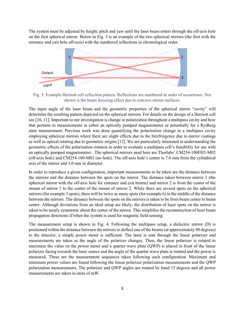
The system must be adjusted by height, pitch and yaw until the laser beam enters through the off-axis hole on the first spherical mirror. Below in Fig. 3 is an example of the two spherical mirrors (the first with the entrance and exit hole off-axis) with the numbered reflections in chronological order.

Fig. 3: Example Herriott cell reflection pattern. Reflections are numbered in order of occurrence. Not shown is the beam focusing effect due to concave mirror surfaces.

The input angle of the laser beam and the geometric properties of the spherical mirror “cavity” will determine the resulting pattern depicted on the spherical mirrors. For details on the design of a Herriott cell see [10, 11]. Important to our investigation is change in polarization throughout a multipass cavity and how that pertains to measurements in either an optically pumped magnetometer or potentially for a Rydberg state measurement. Previous work was done quantifying the polarization change in a multipass cavity employing spherical mirrors where there are slight effects due to the birefringence due to mirror coatings as well as optical rotating due to geometric origins [12]. We are particularly interested in understanding the geometric effects of the polarization rotation in order to evaluate a multipass cell’s feasibility for use with an optically pumped magnetometer. The spherical mirrors used here are Thorlabs’ CM254-100EH3-M02 (off-axis hole) and CM254-100-M02 (no hole). The off-axis hole’s center is 7.0 mm from the cylindrical axis of the mirror and 3.0 mm in diameter.

In order to reproduce a given configuration, important measurements to be taken are the distance between the mirrors and the distance between the spots on the mirror. The distance taken between mirror 1 (the spherical mirror with the off-axis hole for entrance and exit beams) and mirror 2 is from the center of the mount of mirror 1 to the center of the mount of mirror 2. While there are several spots on the spherical mirrors (for example 3 spots), there will be twice as many spots (for example 6) in the middle of the distance between the mirrors. The distance between the spots on the mirrors is taken to be from beam center to beam center. Although deviations from an ideal setup are likely, the distribution of laser spots on the mirror is taken to be nearly symmetric about the center of the mirror. This simplifies the reconstruction of laser beam propagation directions if/when the system is used for magnetic field sensing.

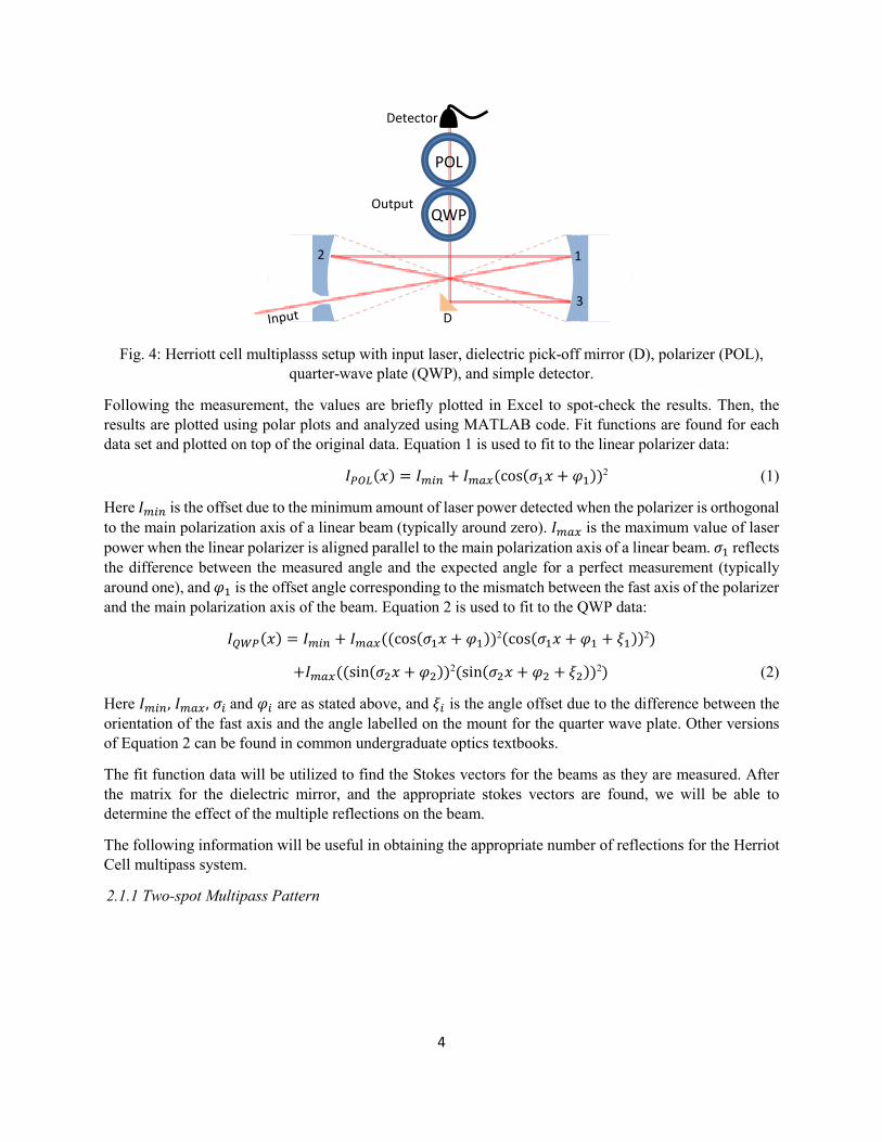
The measurement setup is shown in Fig. 4. Following the multipass setup, a dielectric mirror (D) is positioned within the distance between the mirrors to deflect one of the beams (at approximately 90 degrees) to the detector, a simple power meter is sufficient. The laser is sent through the linear polarizer and measurements are taken as the angle of the polarizer changes. Then, the linear polarizer is rotated to maximize the value on the power meter and a quarter wave plate (QWP) is placed in front of the linear polarizer facing towards the laser source and the angle of the quarter wave plate is rotated and the power is measured. These are the measurement sequences taken following each configuration. Maximum and minimum power values are found following the linear polarizer polarization measurements and the QWP polarization measurements. The polarizer and QWP angles are rotated by hand 15 degrees and all power measurements are taken in units of mW.

Output

1 2

3

4

Fig. 4: Herriott cell multiplasss setup with input laser, dielectric pick-off mirror (D), polarizer (POL), quarter-wave plate (QWP), and simple detector.

Following the measurement, the values are briefly plotted in Excel to spot-check the results. Then, the results are plotted using polar plots and analyzed using MATLAB code. Fit functions are found for each data set and plotted on top of the original data. Equation 1 is used to fit to the linear polarizer data:

𝐼𝐼𝑃𝑃𝑃𝑃𝑃𝑃(𝑥𝑥) = 𝐼𝐼𝑚𝑚𝑚𝑚𝑚𝑚 + 𝐼𝐼𝑚𝑚𝑚𝑚𝑚𝑚(cos(𝜎𝜎1𝑥𝑥 + 𝜑𝜑1))2 (1)

Here 𝐼𝐼𝑚𝑚𝑚𝑚𝑚𝑚 is the offset due to the minimum amount of laser power detected when the polarizer is orthogonal to the main polarization axis of a linear beam (typically around zero). 𝐼𝐼𝑚𝑚𝑚𝑚𝑚𝑚 is the maximum value of laser power when the linear polarizer is aligned parallel to the main polarization axis of a linear beam. 𝜎𝜎1 reflects the difference between the measured angle and the expected angle for a perfect measurement (typically around one), and 𝜑𝜑1 is the offset angle corresponding to the mismatch between the fast axis of the polarizer and the main polarization axis of the beam. Equation 2 is used to fit to the QWP data:

𝐼𝐼𝑄𝑄𝑄𝑄𝑃𝑃(𝑥𝑥) = 𝐼𝐼𝑚𝑚𝑚𝑚𝑚𝑚 + 𝐼𝐼𝑚𝑚𝑚𝑚𝑚𝑚((cos(𝜎𝜎1𝑥𝑥 + 𝜑𝜑1))2(cos(𝜎𝜎1𝑥𝑥 + 𝜑𝜑1 + 𝜉𝜉1))2)

+𝐼𝐼𝑚𝑚𝑚𝑚𝑚𝑚((sin(𝜎𝜎2𝑥𝑥 + 𝜑𝜑2))2(sin(𝜎𝜎2𝑥𝑥 + 𝜑𝜑2 + 𝜉𝜉2))2) (2)

Here 𝐼𝐼𝑚𝑚𝑚𝑚𝑚𝑚, 𝐼𝐼𝑚𝑚𝑚𝑚𝑚𝑚, 𝜎𝜎𝑚𝑚 and 𝜑𝜑𝑚𝑚 are as stated above, and 𝜉𝜉𝑚𝑚 is the angle offset due to the difference between the orientation of the fast axis and the angle labelled on the mount for the quarter wave plate. Other versions of Equation 2 can be found in common undergraduate optics textbooks.

The fit function data will be utilized to find the Stokes vectors for the beams as they are measured. After the matrix for the dielectric mirror, and the appropriate stokes vectors are found, we will be able to determine the effect of the multiple reflections on the beam.

The following information will be useful in obtaining the appropriate number of reflections for the Herriot Cell multipass system. 2.1.1 Two-spot Multipass Pattern

Output

1 2

3 D

QWP

POL

Detector

5

Fig. 5: Herriott cell two-spot multipass (a) reflection pattern and (b) cell pattern.

The reflection pattern and cell pattern can be found for the two-spot multipass setup in Fig. 5a and b respectively. The two spherical mirrors are 20.5 cm apart. The spots are 1.6 cm apart. This is the lowest order configuration of this system where the traversing beams do not overlap. Additionally, the interior angles with respect to the cell axis is quite large. This angle will impact the “orthogonality” of the light-shift beams, pump and probe beams, and magnetic field vector, to the largest degree. We measured all four beams.

2.1.2 Three-spot Multipass Pattern:

The reflection and cell pattern for the three multipass setup is shown in Fig. 6a and b respectively. The two spherical mirrors are 11.8 cm apart. The distance between spots for mirror 1 and 2 are shown in Table 1a and b respectively

Table 1: Distance between spots for (a) mirror 1 and (b) mirror 2 for three-spot multipass.

6

Fig. 6: Herriott cell three-spot multipass (a) reflection pattern and (b) cell pattern.

2.1.3 Four-spot Multipass Pattern:

The two spherical mirrors are 6.7 cm apart. We measured the input beam, beam 1 to 2, 3 to 4, 5 to 6, and the output beam with the measurements found in Table 2. The spot patterns seen on the two mirrors are shown in Fig. 7.

Table 2: Distance between spots for (a) mirror 1 and (b) mirror 2 for four-spot multipass.

7

Fig. 7: Herriott cell four-spot multipass (a) reflection pattern and (b) cell pattern.

2.1.4 Five-spot Multipass Pattern:

Fig. 8: Herriott cell five-spot multipass (a) reflection pattern and (b) cell pattern.

The five multipass pattern can be found with the two spherical mirrors 14.3 cm apart. However, measurements were not taken. The beams in this particular arrangement intersect at the center of the cavity mirrors, where a vapor cell would be positioned. This setup would allow for an interference between pseudo-counter-propagating beams. In Fig .8 are the spot patterns seen on the two mirrors.

2.1.5 Higher-order Multipass Patters:

From the literature [10,11,13], it is clear that the Herriott Cell cavity can hold many multitudes of folded beams. Depending on the initial geometry of the input beam to the cavity, specific patterns are more easily obtained than others. There are drawbacks for using larger numbers of reflections for our purposes, namely intensity concerns. As an example, a beam that is attenuated by some amount through each pass of a vapor cell would require significantly higher power to start with to be able to traverse the vapor cell many more

8

times. As multiplying the power for a probe beam in a pump-probe experiment would disturb the nature of the interactions taking place, larger numbers of reflections would cause a problem. In another manor, much like the five-spot multipass system shown in Fig. 8, there exist beam patterns that produce overlapping beams within the vapor cell that could cause interference in signal acquisition, again something to be avoided for our interest in OPMs and Rydberg electrometry.

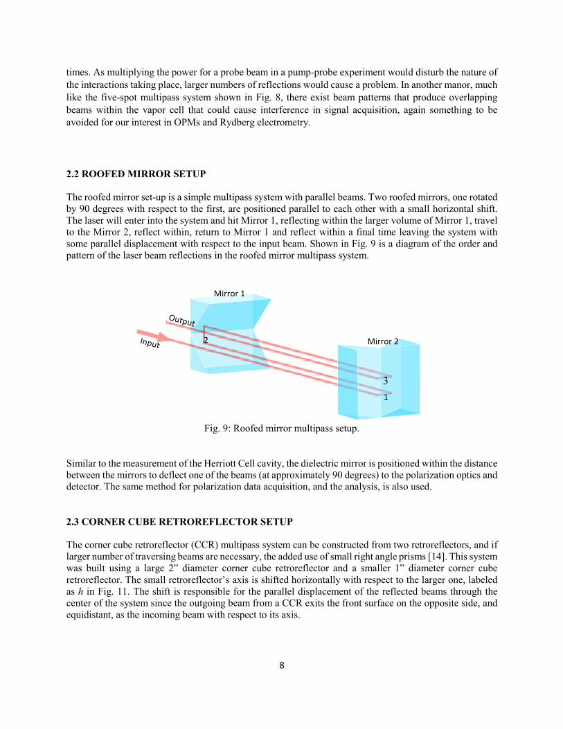
2.2 ROOFED MIRROR SETUP The roofed mirror set-up is a simple multipass system with parallel beams. Two roofed mirrors, one rotated by 90 degrees with respect to the first, are positioned parallel to each other with a small horizontal shift. The laser will enter into the system and hit Mirror 1, reflecting within the larger volume of Mirror 1, travel to the Mirror 2, reflect within, return to Mirror 1 and reflect within a final time leaving the system with some parallel displacement with respect to the input beam. Shown in Fig. 9 is a diagram of the order and pattern of the laser beam reflections in the roofed mirror multipass system.

Fig. 9: Roofed mirror multipass setup.

Similar to the measurement of the Herriott Cell cavity, the dielectric mirror is positioned within the distance between the mirrors to deflect one of the beams (at approximately 90 degrees) to the polarization optics and detector. The same method for polarization data acquisition, and the analysis, is also used.

2.3 CORNER CUBE RETROREFLECTOR SETUP The corner cube retroreflector (CCR) multipass system can be constructed from two retroreflectors, and if larger number of traversing beams are necessary, the added use of small right angle prisms [14]. This system was built using a large 2” diameter corner cube retroreflector and a smaller 1” diameter corner cube retroreflector. The small retroreflector’s axis is shifted horizontally with respect to the larger one, labeled as h in Fig. 11. The shift is responsible for the parallel displacement of the reflected beams through the center of the system since the outgoing beam from a CCR exits the front surface on the opposite side, and equidistant, as the incoming beam with respect to its axis.

Mirror 1

Mirror 2

1

2

3

9

Fig. 11: Diagram of the order and pattern of the laser beam reflection in the CCR multipass system. For simplicity, reflections internal to the CCRs are not shown. h is the displacement between the two CCR

reflecting axes.

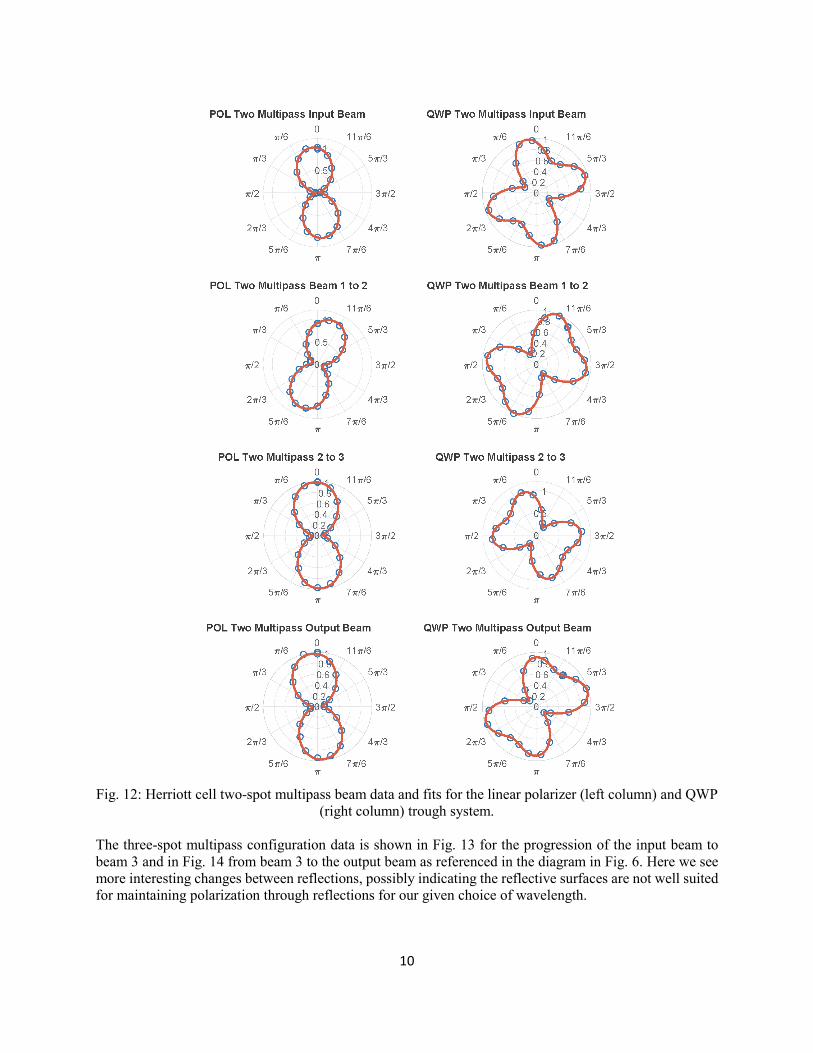
The large retroreflector is facing towards the input laser beam. As the beam enters the large retroreflector, it reflects from each of the three back surfaces and exits across the center of the retroreflector from where it entered. Then it traverse the distance between the CCRs, where a vapor cell could be, and enters the small retroreflector. The back and forth between CCRs continues until the beam can pass outside of the front surface area of the smaller retroreflector. Thus, with some clever positioning, as few as four traversing beams can be implemented. For the OPM, magnetic field gradients could be a problem, so ensuring the pattern is relatively square or evenly spaced would be beneficial. As before, the dielectric mirror is positioned within the distance between the retroreflectors to deflect one of the beams (at approximately 90 degrees) to the polarization optics and detector. The same method for polarization data acquisition, and the analysis, is also used. 3 POLAR PLOT RESULTS We will first look at the Herriott Cell cavity results. Looking at the two-spot multipass setup, the plots for the linear polarizer and quarter wave plate are shown in Fig. 12 on the left and right columns respectively. These plots show that the less-steep reflection angles in this configuration cause slight changes to the orientation of the beam polarization. As expected, the handedness of the should change upon a single reflection .

1

2

Output Input

3

4

h

10

Fig. 12: Herriott cell two-spot multipass beam data and fits for the linear polarizer (left column) and QWP

(right column) trough system.

The three-spot multipass configuration data is shown in Fig. 13 for the progression of the input beam to beam 3 and in Fig. 14 from beam 3 to the output beam as referenced in the diagram in Fig. 6. Here we see more interesting changes between reflections, possibly indicating the reflective surfaces are not well suited for maintaining polarization through reflections for our given choice of wavelength.

11

Fig. 13: Herriott cell three-spot multipass beam data and fits for the linear polarizer (left column) and

QWP (right column) for Input beam through to beam 3.

12

Fig. 14: Herriott cell three-spot multipass beam data and fits for the linear polarizer (left column) and

QWP (right column) for beam 3 to output.

13

Fig. 15: Herriott cell four-spot multipass beam data and fits for the linear polarizer (left column) and

QWP (right column) for Input beam through to beam 4.

The four-spot multipass configuration data can be seen in Fig. 15 and Fig. 16. Again, there is some slight wiggling of the orientation of the linear polarization of the laser. In addition, we can clearly see the change of elliptical polarization is the beam progresses in the multipass system.

14

Fig. 16: Herriott cell four-spot multipass beam data and fits for the linear polarizer (left column) and

QWP (right column) for beam 5 to output.

15

Fig. 17: Roofed mirror data and fits for linear polarizer (left column) and QWP (right column) for input to

output.

Similar to the plots above for the Herriott cell, the roofed mirror cell results are plotted in Fig. 17. The reflections within the volume of the roofed mirrors are about 45 degrees from normal to the reflective surfaces. This far from normal incidence is expected to cause some mixing of the linear polarization. Unexpectedly, the elliptical polarization of the beam changes symmetrically, from one mirror to the other.

16

Fig. 18: CCR data and fits for linear polarizer (left column) and QWP (right column) from input to

output, for the minimum of four traversing beams.

The plots for the CCR cavity are shown in Fig. 18. In this case the variations are more subtle. Where the incoming beam was linearly polarized, the outgoing beam from a CCR is elliptically polarized. Thus, multiple reflections within a CCR-based cavity quickly complicate the laser beam polarization making it difficult to employ practically for use with the optically pumped magnetometer and possibly for the

17

Rydberg electrometry experiments. For this reason the CCR is ruled out for our purposes as a method to increase signal to noise.

4 SUMMARY AND CONCLUSIONS In summary we investigated the polarization rotation in a number of multipass cells for evaluation in employing them for both the optically pumped magnetometer and for Rydberg electric field sensing. The results indicate that the CCR multipass cell is not suitable for use. The roofed mirror behaves as expected but lacks in the number of reflections we can achieve in a simple setup and therefore limits the potential gain in SNR which is desired. The Herriott cell promises the most potential for future use but would still require rigorous analysis of the polarization rotation through the cell especially if we desire to increase the number of reflections that are utilized. The potential for utilization in the optically pumped magnetometer relies on resolving any effects on the measurement approach which relies on detection of a nonlinear magneto-optical rotation of the polarization. A potential approach to handle this technical challenge would involve theoretical development of propagation and reflection effects in the cell, which have been studied previously for other applications with matrix methods, similar to the theory of [13], with additional information from OPM studies. REFERENCES 1. J. W. Lou and G. A. Cranch, “Characterization of atomic spin polarization lifetime of cesium vapor cells with neon buffer gas,” AIP Advances, 8, 025305, 1-8 (2018). 2. H. Fan, S. Kumar, J. Sedlacek, H. Kubler, S. Karimkashi, and J. P. Shaffer, “Atom based RF electric field sensing,” J. Phys. B: At. Mol. Opt. Phys., 48, 202001, 1-16 (2015). 3. A. Foltynowicz, P. Maslowski, T. Ban, F. Adler, K. C. Cossel, T. C. Briles, and J. Ye, “Optical frequency comb spectroscopy,” Royal Society of Chemistry, 150, 23-31 (2011). 4. M. Graf, L. Emmenegger, and B. Tuzson, “Compact, circular, and optically stable multipass cell for mobile laser absorption spectroscopy,” Opt. Lett., 43, 11, 2434-2437 (2018). 5. P. Guay, J. Genest, and A. J. Fleisher, “Precision spectroscopy of H13CN using a free-running, all-fiber dual electro-optic frequency comb system,” Opt. Lett., 43, 6, 1407-1410 (2018). 6. B. A. Paldus and A. A. Kachanov, “An historical overview of cavity-enhanced methods,” Can. J. Phys., 83, 975-999 (2005). 7. S. Li, P. Vachaspati, D. Sheng, N. Dural, and M. V. Romalis, “Optical rotation in excess of 100 rad generated by Rb vapor in a multipass cell,” Phys. Rev. A, 84, 061403, 1-4 (2011). 8. D. Sheng, S. Li, N. Dural, and M. V. Romalis, “Subfemtotesla Scalar Atomic Magnetometry Using Multipass Cells,” Phys. Rev. Lett., 110, 160802, 1-5 (2013). 9. M. A. Bouchiat, L. Pottier, Gerard Trenec. A cesium cell with laser beam multipass. Revue de Physique Appliquee, 1980, 15 (3), pp.785-788. <10.1051/rphysap:01980001503078500>.

18

10. D. Herriott, H. Kogelnik, and R. Kompfner, “Off-Axis Paths in Spherical Mirror Interferometers,” App. Opt., 3, 4, 523-525 (1964). 11. J. Altmann, R. Baumgart, and C. Weitkamp, “Two-mirror multipass absorption cell,” App. Opt., 20, 6, 995-999 (1981). 12. M. A. Bouchiat and L. Pottier, “Light-polarization Modifications in a Multipass Cavity,” App. Phys. B, 29, 43-54 (1982). 13. J. B. McManus, P. L. Kebabian, and M. S. Zahniser, “Astimatic mirror multipass absorption cells for long-path-length spectroscopy,” App. Opt., 34, 18, 3336-3348 (1995). 14. A. L. Vitushkin and L. F. Vitushkin, “Design of a multipass optical cell based on the use of shifted corner cubes and right-angle prisms,” App. Opt., 37, 1, 162-165 (1998).

19

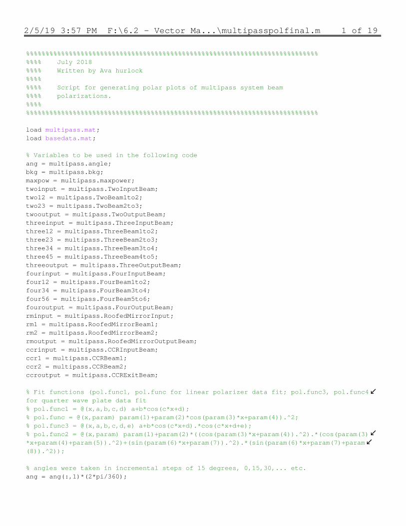
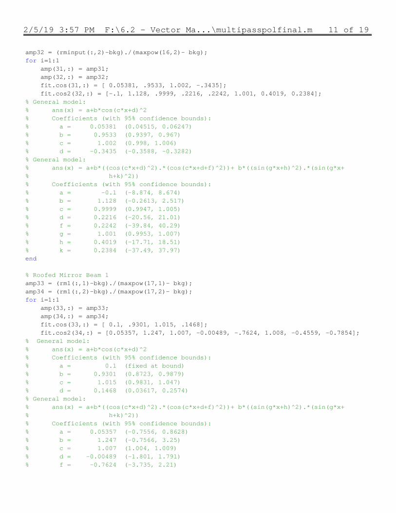
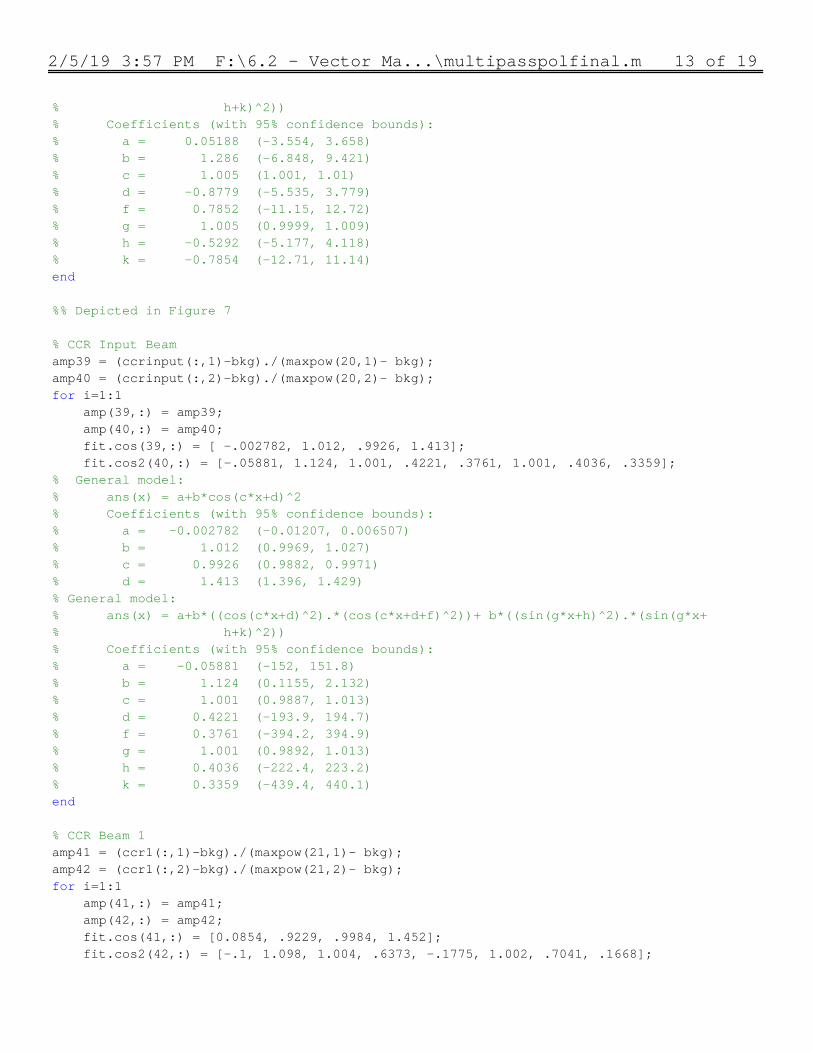
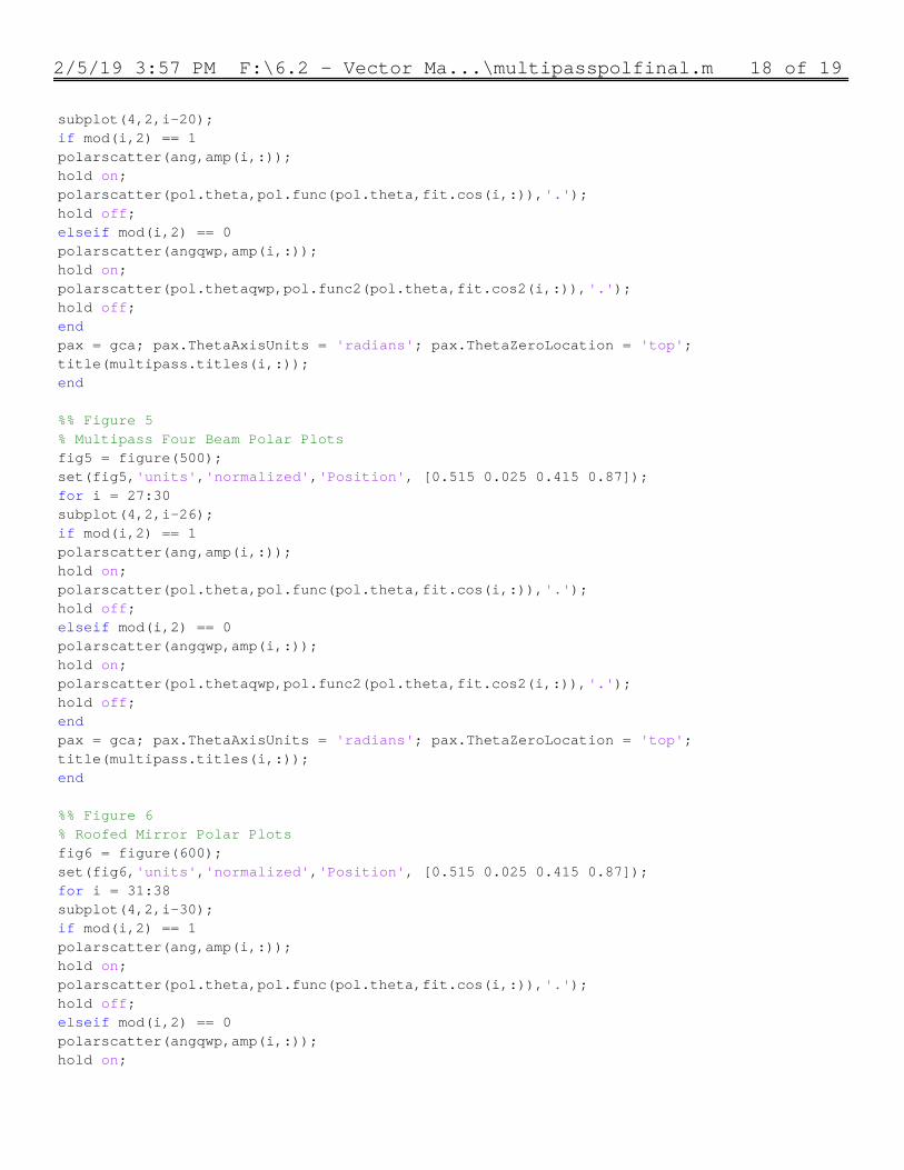
APPENDIX A: CODE The complete Matlab code used to calculate the polar plots in Section 3 can be found below. The code relies on the multipass.mat and basedata.mat files which contain the data specific to these graphs which is not included. However the comments detail a general model and it should be straightforward to replicate with similar data collection methods as detailed in Section 2.

2/5/19 3:57 PM F:\6.2 - Vector Ma...\multipasspolfinal.m 1 of 19

%%%%%%%%%%%%%%%%%%%%%%%%%%%%%%%%%%%%%%%%%%%%%%%%%%%%%%%%%%%%%%%%%%%%%%%%%%%%%%% July 2018%%%% Written by Ava hurlock%%%% %%%% Script for generating polar plots of multipass system beam%%%% polarizations.%%%%%%%%%%%%%%%%%%%%%%%%%%%%%%%%%%%%%%%%%%%%%%%%%%%%%%%%%%%%%%%%%%%%%%%%%%%%%%% load multipass.mat;load basedata.mat; % Variables to be used in the following codeang = multipass.angle;bkg = multipass.bkg;maxpow = multipass.maxpower;twoinput = multipass.TwoInputBeam;two12 = multipass.TwoBeam1to2;two23 = multipass.TwoBeam2to3;twooutput = multipass.TwoOutputBeam;threeinput = multipass.ThreeInputBeam;three12 = multipass.ThreeBeam1to2;three23 = multipass.ThreeBeam2to3;three34 = multipass.ThreeBeam3to4;three45 = multipass.ThreeBeam4to5;threeoutput = multipass.ThreeOutputBeam;fourinput = multipass.FourInputBeam;four12 = multipass.FourBeam1to2;four34 = multipass.FourBeam3to4;four56 = multipass.FourBeam5to6;fouroutput = multipass.FourOutputBeam;rminput = multipass.RoofedMirrorInput;rm1 = multipass.RoofedMirrorBeam1;rm2 = multipass.RoofedMirrorBeam2;rmoutput = multipass.RoofedMirrorOutputBeam;ccrinput = multipass.CCRInputBeam;ccr1 = multipass.CCRBeam1;ccr2 = multipass.CCRBeam2;ccroutput = multipass.CCRExitBeam; % Fit functions (pol.func1, pol.func for linear polarizer data fit; pol.func3, pol.func4 for quarter wave plate data fit % pol.func1 = @(x,a,b,c,d) a+b*cos(c*x+d);% pol.func = @(x,param) param(1)+param(2)*cos(param(3)*x+param(4)).^2;% pol.func3 = @(x,a,b,c,d,e) a+b*cos(c*x+d).*cos(c*x+d+e);% pol.func2 = @(x,param) param(1)+param(2)*((cos(param(3)*x+param(4)).^2).*(cos(param(3)*x+param(4)+param(5)).^2)+(sin(param(6)*x+param(7)).^2).*(sin(param(6)*x+param(7)+param(8)).^2)); % angles were taken in incremental steps of 15 degrees, 0,15,30,... etc.ang = ang(:,1)*(2*pi/360);


% For the correct orientation of the QWP, the angles must be subtracted by% 40 degreesangqwp = ang - (2*pi/360)*40; % Pol.thetaqwp corrects the theta for use in the QWP fit functions by% subtracting 40 degreespol.thetaqwp = pol.theta - (2*pi/360)*40; %% Depicted in Figure 1 % Two Multipass Input Beamamp1 = (twoinput(:,1)-bkg)./(maxpow(1,1)- bkg);amp2 = (twoinput(:,2)-bkg)./(maxpow(1,2)- bkg);for i=1:1 amp(1,:) = amp1; amp(2,:) = amp2; fit.cos(1,:) = [.03202, .9714, .9986, -.1212]; fit.cos2(2,:) = [.09003, 1.167, 1.004, .07599, .7854, 1.003, .3399, .7244]; %fit.cos2(2,:) = [a, b, c, d, f, g, h, k];% General model:% ans(x) = a+b*cos(c*x+d)^2% Coefficients (with 95% confidence bounds):% a = 0.03202 (0.02273, 0.0413)% b = 0.9714 (0.9567, 0.986)% c = 0.9986 (0.994, 1.003)% d = -0.1212 (-0.1382, -0.1043)% General model:% ans(x) = a+b*((cos(c*x+d)^2).*(cos(c*x+d+f)^2))+ b*((sin(g*x+h)^2).*(sin(g*x+% h+k)^2))% Coefficients (with 95% confidence bounds):% a = 0.09003 (-6.944, 7.124)% b = 1.167 (-1.931, 4.266)% c = 1.004 (0.9995, 1.008)% d = 0.07599 (-8.413, 8.565)% f = 0.7854 (-13.52, 15.09)% g = 1.003 (0.9983, 1.008)% h = 0.3399 (-6.013, 6.693)% k = 0.7244 (-14.66, 16.11)end % Two Multipass Beam 1 to 2amp3 = (two12(:,1)-bkg)./(maxpow(2,1)- bkg);amp4 = (two12(:,2)-bkg)./(maxpow(2,2)- bkg);for i=1:1 amp(3,:) = amp3; amp(4,:) = amp4; fit.cos(3,:) = [.1, .9203, 1.005, .3326]; fit.cos2(4,:) = [-0.04818, 1.034, 1.002, -0.2927, 0, 1, -0.3758, -0.3789];% General model:% ans(x) = a+b*cos(c*x+d)^2


% Coefficients (with 95% confidence bounds):% a = 0.1 (fixed at bound)% b = 0.9203 (0.8995, 0.9411)% c = 1.005 (0.9937, 1.015)% d = 0.3326 (0.2952, 0.3701)% General model:% ans(x) = a+b*((cos(c*x+d)^2).*(cos(c*x+d+f)^2))+ b*((sin(g*x+h)^2).*(sin(g*x+% h+k)^2))% Coefficients (with 95% confidence bounds):% a = -0.04818 (-1.369, 1.273)% b = 1.034 (0.5653, 1.504)% c = 1.002 (0.9997, 1.005)% d = -0.2927 (-1.302e+04, 1.302e+04)% f = -6.428e-05 (-2.603e+04, 2.603e+04)% g = 1 (fixed at bound)% h = -0.3758 (-2.419, 1.667)% k = -0.3789 (-4.83, 4.072)end % Two Multipass Beam 2 to 3amp5 = (two23(:,1)-bkg)./(maxpow(3,1)- bkg);amp6 = (two23(:,2)-bkg)./(maxpow(3,2)- bkg);for i=1:1 amp(5,:) = amp5; amp(6,:) = amp6; fit.cos(5,:) = [ 0.1, .885, 1.006, -.07694]; fit.cos2(6,:) = [-.06857, 1.094, 1, .6733, .2856, 1, .6692, -.2061];% General model:% ans(x) = a+b*cos(c*x+d)^2% Coefficients (with 95% confidence bounds):% a = 0.1 (fixed at bound)% b = 0.885 (0.8759, 0.8942)% c = 1.006 (1.001, 1.011)% d = -0.07694 (-0.09611, -0.05778)% General model:% ans(x) = a+b*((cos(c*x+d)^2).*(cos(c*x+d+f)^2))+ b*((sin(g*x+h)^2).*(sin(g*x+% h+k)^2))% Coefficients (with 95% confidence bounds):% a = -0.06857 (-32.24, 32.1)% b = 1.094 (-7.914, 10.1)% c = 1 (0.9932, 1.007)% d = 0.6733 (-60.16, 61.51)% f = 0.2856 (-128.9, 129.4)% g = 1 (fixed at bound)% h = 0.6692 (-84.79, 86.12)% k = -0.2061 (-178.6, 178.2)end % Two Multipass Output Beamamp7 = (twooutput(:,1)-bkg)./(maxpow(4,1)- bkg);amp8 = (twooutput(:,2)-bkg)./(maxpow(4,2)- bkg);


for i=1:1 amp(7,:) = amp7; amp(8,:) = amp8; fit.cos(7,:) = [ 0.1, .8764, 1.005, -.1253]; fit.cos2(8,:) = [0.07599, 1.14, 1.001, 0.2051, .6859, 1.004, 0.487, .7854];% General model:% ans(x) = a+b*cos(c*x+d)^2% Coefficients (with 95% confidence bounds):% a = 0.1 (fixed at bound)% b = 0.8764 (0.8653, 0.8874)% c = 1.005 (0.9982, 1.011)% d = -0.1253 (-0.1488, -0.1018)% General model:% ans(x) = a+b*((cos(c*x+d)^2).*(cos(c*x+d+f)^2))+ b*((sin(g*x+h)^2).*(sin(g*x+% h+k)^2))% Coefficients (with 95% confidence bounds):% a = 0.07599 (-0.6283, 0.7803)% b = 1.14 (0.4089, 1.872)% c = 1.001 (0.9973, 1.004)% d = 0.2051 (-1.017, 1.427)% f = 0.6859 (-1.371, 2.742)% g = 1.004 (1, 1.008)% h = 0.487 (-0.2214, 1.195)% k = 0.7854 (-1.015, 2.585)end %% Depicted in Figure 2 % Three Multipass Input Beamamp9 = (threeinput(:,1)-bkg)./(maxpow(5,1)- bkg);amp10 = (threeinput(:,2)-bkg)./(maxpow(5,2)- bkg);for i=1:1 amp(9,:) = amp9; amp(10,:) = amp10; fit.cos(9,:) = [ 0.06751, .9282, .9966, .2714]; fit.cos2(10,:) = [.1, 1.171, 1.003, -0.7593, .7197, 1.005, -0.3131, -.7441];% General model:% ans(x) = a+b*cos(c*x+d)^2% Coefficients (with 95% confidence bounds):% a = 0.06751 (0.06269, 0.07232)% b = 0.9282 (0.9206, 0.9358)% c = 0.9966 (0.9942, 0.999)% d = 0.2714 (0.2631, 0.2797)% General model:% ans(x) = a+b*((cos(c*x+d)^2).*(cos(c*x+d+f)^2))+ b*((sin(g*x+h)^2).*(sin(g*x+% h+k)^2))% Coefficients (with 95% confidence bounds):% a = 0.1 (fixed at bound)% b = 1.171 (1.144, 1.198)% c = 1.003 (0.9999, 1.006)% d = -0.7593 (-0.7765, -0.7422)


% f = 0.7197 (0.6919, 0.7475)% g = 1.005 (1.001, 1.008)% h = -0.3131 (-0.3339, -0.2924)% k = -0.7441 (-0.7713, -0.7169)end % Three Multipass Beam 1 to 2amp11 = (three12(:,1)-bkg)./(maxpow(6,1)- bkg);amp12 = (three12(:,2)-bkg)./(maxpow(6,2)- bkg);for i=1:1 amp(11,:) = amp11; amp(12,:) = amp12; fit.cos(11,:) = [ 0.1, .9149, 1.001, -.06767]; fit.cos2(12,:) = [-.06251, 1.061, .9985, .7327, .3089, 1, 0.6772, -.1228];% General model:% ans(x) = a+b*cos(c*x+d)^2% Coefficients (with 95% confidence bounds):% a = 0.1 (fixed at bound)% b = 0.9149 (0.903, 0.9267)% c = 1.001 (0.9948, 1.008)% d = -0.06767 (-0.09156, -0.04379)% General model:% ans(x) = a+b*((cos(c*x+d)^2).*(cos(c*x+d+f)^2))+ b*((sin(g*x+h)^2).*(sin(g*x+% h+k)^2))% Coefficients (with 95% confidence bounds):% a = -0.06251 (-3.252, 3.127)% b = 1.061 (0.0513, 2.071)% c = 0.9985 (0.9931, 1.004)% d = 0.7327 (-5.076, 6.542)% f = 0.3089 (-12.14, 12.76)% g = 1 (fixed at bound)% h = 0.6772 (-14.48, 15.84)% k = -0.1228 (-31.25, 31)end % Three Multipass Beam 2 to 3amp13 = (three23(:,1)-bkg)./(maxpow(7,1)- bkg);amp14 = (three23(:,2)-bkg)./(maxpow(7,2)- bkg);for i=1:1 amp(13,:) = amp13; amp(14,:) = amp14; fit.cos(13,:) = [ 0.03667, 1.604, 1.004, -.1681]; fit.cos2(14,:) = [0.09999, .9265, 1.006, 0.4661, .0003666, 1.005, 0.616, 0];% General model:% ans(x) = a+b*cos(c*x+d)^2% Coefficients (with 95% confidence bounds):% a = 0.03667 (0.01905, 0.0543)% b = 1.604 (1.576, 1.632)% c = 1.004 (0.999, 1.01)% d = -0.1681 (-0.1875, -0.1487)% General model:


% ans(x) = a+b*((cos(c*x+d)^2).*(cos(c*x+d+f)^2))+ b*((sin(g*x+h)^2).*(sin(g*x+% h+k)^2))% Coefficients (with 95% confidence bounds):% a = 0.09999 (-0.4624, 0.6624)% b = 0.9265 (0.8586, 0.9943)% c = 1.006 (0.9952, 1.016)% d = 0.4661 (-807.4, 808.3)% f = 0.0003666 (-1616, 1616)% g = 1.005 (0.9918, 1.018)% h = 0.616 (-1.682e+06, 1.682e+06)% k = 1.82e-07 (-3.364e+06, 3.364e+06)end %% Depicted in Figure 3 % Three Multipass Beam 3 to 4amp15 = (three34(:,1)-bkg)./(maxpow(8,1)- bkg);amp16 = (three34(:,2)-bkg)./(maxpow(8,2)- bkg);for i=1:1 amp(15,:) = amp15; amp(16,:) = amp16; fit.cos(15,:) = [ 0.1, .8857, 1.011, .01331]; fit.cos2(16,:) = [-.05696, 1.046, 1.004, -.6693, -.3267, 1, -.5853, 0];% General model:% ans(x) = a+b*cos(c*x+d)^2% Coefficients (with 95% confidence bounds):% a = 0.1 (fixed at bound)% b = 0.8857 (0.877, 0.8945)% c = 1.011 (1.006, 1.016)% d = 0.01331 (-0.004955, 0.03158)% General model:% ans(x) = a+b*((cos(c*x+d)^2).*(cos(c*x+d+f)^2))+ b*((sin(g*x+h)^2).*(sin(g*x+% h+k)^2))% Coefficients (with 95% confidence bounds):% a = -0.05696 (-3.556, 3.442)% b = 1.046 (0.1909, 1.901)% c = 1.004 (0.9896, 1.018)% d = -0.6693 (-6.497, 5.159)% f = -0.3267 (-12.85, 12.2)% g = 1 (fixed at bound)% h = -0.5853 (-3.333e+04, 3.333e+04)% k = 6.085e-05 (-6.666e+04, 6.666e+04)end % Three Multipass Beam 4 to 5amp17 = (three45(:,1)-bkg)./(maxpow(9,1)- bkg);amp18 = (three45(:,2)-bkg)./(maxpow(9,2)- bkg);for i=1:1 amp(17,:) = amp17; amp(18,:) = amp18; fit.cos(17,:) = [ 0.07903, .9181, 1.001, .264];


fit.cos2(18,:) = [0.1, 1.166, .9954, -.7586, .7033, 1, -0.3264, -.7357];% General model:% ans(x) = a+b*cos(c*x+d)^2% Coefficients (with 95% confidence bounds):% a = 0.07903 (0.07116, 0.0869)% b = 0.9181 (0.9057, 0.9305)% c = 1.001 (0.9973, 1.005)% d = 0.264 (0.2504, 0.2776)% General model:% ans(x) = a+b*((cos(c*x+d)^2).*(cos(c*x+d+f)^2))+ b*((sin(g*x+h)^2).*(sin(g*x+% h+k)^2))% Coefficients (with 95% confidence bounds):% a = 0.1 (-1.114, 1.314)% b = 1.166 (0.4422, 1.89)% c = 0.9954 (0.9892, 1.002)% d = -0.7586 (-1.903, 0.3853)% f = 0.7033 (-2.119, 3.526)% g = 1 (fixed at bound)% h = -0.3264 (-1.433, 0.78)% k = -0.7357 (-3.45, 1.979)end % Three Multipass Output Beamamp19 = (threeoutput(:,1)-bkg)./(maxpow(10,1)- bkg);amp20 = (threeoutput(:,2)-bkg)./(maxpow(10,2)- bkg);for i=1:1 amp(19,:) = amp19; amp(20,:) = amp20; fit.cos(19,:) = [ 0.0007732, .9508, 1.007, .2167]; fit.cos2(20,:) = [0.07867, 1.239, 1.002, -0.2589, -.7155, 1.003, -.3594, -.7854];% General model:% ans(x) = a+b*cos(c*x+d)^2% Coefficients (with 95% confidence bounds):% a = 0.0007732 (-0.02252, 0.02407)% b = 0.9508 (0.9143, 0.9873)% c = 1.007 (0.9952, 1.018)% d = 0.2167 (0.1772, 0.2562)% General model:% ans(x) = a+b*((cos(c*x+d)^2).*(cos(c*x+d+f)^2))+ b*((sin(g*x+h)^2).*(sin(g*x+% h+k)^2))% Coefficients (with 95% confidence bounds):% a = 0.07867 (0.04643, 0.1109)% b = 1.239 (1.182, 1.296)% c = 1.002 (0.9949, 1.01)% d = -0.2589 (-0.2892, -0.2285)% f = -0.7155 (-0.7532, -0.6778)% g = 1.003 (0.9943, 1.012)% h = -0.3594 (-0.3954, -0.3234)% k = -0.7854 (fixed at bound))end


%% Depicted in Figure 4 % Four Multipass Input Beamamp21 = (fourinput(:,1)-bkg)./(maxpow(11,1)- bkg);amp22 = (fourinput(:,2)-bkg)./(maxpow(11,2)- bkg);for i=1:1 amp(21,:) = amp21; amp(22,:) = amp22; fit.cos(21,:) = [ 0.03326, .9666, .998, .2022]; fit.cos2(22,:) = [-.09083, 1.096, 1.001, -0.668, -.01839, 1.002, -0.4443, -.2165];% General model:% ans(x) = a+b*cos(c*x+d)^2% Coefficients (with 95% confidence bounds):% a = 0.03326 (0.02332, 0.0432)% b = 0.9666 (0.9509, 0.9822)% c = 0.998 (0.9931, 1.003)% d = 0.2022 (0.1853, 0.2191)% General model:% ans(x) = a+b*((cos(c*x+d)^2).*(cos(c*x+d+f)^2))+ b*((sin(g*x+h)^2).*(sin(g*x+% h+k)^2))% Coefficients (with 95% confidence bounds):% a = -0.09083 (-32.14, 31.96)% b = 1.096 (-1.044, 3.235)% c = 1.001 (0.9879, 1.015)% d = -0.668 (-844.1, 842.8)% f = -0.01839 (-1691, 1691)% g = 1.002 (0.9895, 1.014)% h = -0.4443 (-74.54, 73.65)% k = -0.2165 (-144.7, 144.3)end % Four Multipass Beam 1 to 2amp23 = (four12(:,1)-bkg)./(maxpow(12,1)- bkg);amp24 = (four12(:,2)-bkg)./(maxpow(12,2)- bkg);for i=1:1 amp(23,:) = amp23; amp(24,:) = amp24; fit.cos(23,:) = [ 0.03779, .9524, 1, -.1645]; fit.cos2(24,:) = [0.09997, 1.036, 1.005, 0.3, .6117, 1.003, 0.3617, .5556];% General model:% ans(x) = a+b*cos(c*x+d)^2% Coefficients (with 95% confidence bounds):% a = 0.03779 (0.0286, 0.04699)% b = 0.9524 (0.9379, 0.9669)% c = 1 (0.9954, 1.005)% d = -0.1645 (-0.1816, -0.1474)% General model:% ans(x) = a+b*((cos(c*x+d)^2).*(cos(c*x+d+f)^2))+ b*((sin(g*x+h)^2).*(sin(g*x+% h+k)^2))% Coefficients (with 95% confidence bounds):% a = 0.09997 (-30.08, 30.28)


% b = 1.036 (0.896, 1.177)% c = 1.005 (0.9679, 1.042)% d = 0.3 (-30.88, 31.48)% f = 0.6117 (-60.36, 61.58)% g = 1.003 (0.9651, 1.041)% h = 0.3617 (-32.12, 32.85)% k = 0.5556 (-65.82, 66.93)end % Four Multipass Beam 3 to 4amp25 = (four34(:,1)-bkg)./(maxpow(13,1)- bkg);amp26 = (four34(:,2)-bkg)./(maxpow(13,2)- bkg);for i=1:1 amp(25,:) = amp25; amp(26,:) = amp26; fit.cos(25,:) = [ 0.03569, .974, .9998, -.2036]; fit.cos2(26,:) = [-.03471, 1.073, 1.003, 0.4192, .2906, 1.003, 0.4113, .2715];% General model:% ans(x) = a+b*cos(c*x+d)^2% Coefficients (with 95% confidence bounds):% a = 0.03569 (0.02907, 0.04231)% b = 0.974 (0.9636, 0.9845)% c = 0.9998 (0.9966, 1.003)% d = -0.2036 (-0.2155, -0.1916)% General model:% ans(x) = a+b*((cos(c*x+d)^2).*(cos(c*x+d+f)^2))+ b*((sin(g*x+h)^2).*(sin(g*x+% h+k)^2))% Coefficients (with 95% confidence bounds):% a = -0.03471 (-430.4, 430.3)% b = 1.073 (0.5642, 1.582)% c = 1.003 (0.9377, 1.068)% d = 0.4192 (-724.7, 725.5)% f = 0.2906 (-1458, 1458)% g = 1.003 (0.9389, 1.067)% h = 0.4113 (-782.3, 783.2)% k = 0.2715 (-1558, 1558)end %% Depicted in Figure 5 % Four Multipass Beam 5 to 6amp27 = (four56(:,1)-bkg)./(maxpow(14,1)- bkg);amp28 = (four56(:,2)-bkg)./(maxpow(14,2)- bkg);for i=1:1 amp(27,:) = amp27; amp(28,:) = amp28; fit.cos(27,:) = [ 0.06438, .9376, 1.002, -.03248]; fit.cos2(28,:) = [0.1, 1.197, .9922, .5338, .7539, 1, 0.9828, -0.742];% General model:% ans(x) = a+b*cos(c*x+d)^2% Coefficients (with 95% confidence bounds):


% a = 0.06438 (0.05569, 0.07306)% b = 0.9376 (0.924, 0.9513)% c = 1.002 (0.9972, 1.006)% d = -0.03248 (-0.04888, -0.01608)% General model:% ans(x) = a+b*((cos(c*x+d)^2).*(cos(c*x+d+f)^2))+ b*((sin(g*x+h)^2).*(sin(g*x+% h+k)^2))% Coefficients (with 95% confidence bounds):% a = 0.1 (fixed at bound)% b = 1.197 (1.154, 1.24)% c = 0.9922 (0.9872, 0.9973)% d = 0.5338 (0.5047, 0.563)% f = 0.7539 (0.7127, 0.795)% g = 1 (fixed at bound)% h = 0.9828 (0.9598, 1.006)% k = -0.742 (-0.7839, -0.7002)end % Four Multipass Beam Output Beamamp29 = (fouroutput(:,1)-bkg)./(maxpow(15,1)- bkg);amp30 = (fouroutput(:,2)-bkg)./(maxpow(15,2)- bkg);for i=1:1 amp(29,:) = amp29; amp(30,:) = amp30; fit.cos(29,:) = [ 0.04813, .9431, 1.007, -.06733]; fit.cos2(30,:) = [0.1, 1.207, .9992, .4841, 0.7634, 1, 0.2129, .7523];% General model:% ans(x) = a+b*cos(c*x+d)^2% Coefficients (with 95% confidence bounds):% a = 0.04813 (0.04059, 0.05567)% b = 0.9431 (0.9313, 0.9549)% c = 1.007 (1.003, 1.011)% d = -0.06733 (-0.08152, -0.05314)% General model:% ans(x) = a+b*((cos(c*x+d)^2).*(cos(c*x+d+f)^2))+ b*((sin(g*x+h)^2).*(sin(g*x+% h+k)^2))% Coefficients (with 95% confidence bounds):% a = 0.1 (fixed at bound)% b = 1.207 (1.169, 1.245)% c = 0.9992 (0.9948, 1.003)% d = 0.4841 (0.4586, 0.5096)% f = 0.7634 (0.7279, 0.7989)% g = 1 (fixed at bound)% h = 0.2129 (0.1921, 0.2337)% k = 0.7523 (0.7161, 0.7885)end %% Depicted in Figure 6 % Roofed Mirror Input Beamamp31 = (rminput(:,1)-bkg)./(maxpow(16,1)- bkg);


amp32 = (rminput(:,2)-bkg)./(maxpow(16,2)- bkg);for i=1:1 amp(31,:) = amp31; amp(32,:) = amp32; fit.cos(31,:) = [ 0.05381, .9533, 1.002, -.3435]; fit.cos2(32,:) = [-.1, 1.128, .9999, .2216, .2242, 1.001, 0.4019, 0.2384];% General model:% ans(x) = a+b*cos(c*x+d)^2% Coefficients (with 95% confidence bounds):% a = 0.05381 (0.04515, 0.06247)% b = 0.9533 (0.9397, 0.967)% c = 1.002 (0.998, 1.006)% d = -0.3435 (-0.3588, -0.3282)% General model:% ans(x) = a+b*((cos(c*x+d)^2).*(cos(c*x+d+f)^2))+ b*((sin(g*x+h)^2).*(sin(g*x+% h+k)^2))% Coefficients (with 95% confidence bounds):% a = -0.1 (-8.874, 8.674)% b = 1.128 (-0.2613, 2.517)% c = 0.9999 (0.9947, 1.005)% d = 0.2216 (-20.56, 21.01)% f = 0.2242 (-39.84, 40.29)% g = 1.001 (0.9953, 1.007)% h = 0.4019 (-17.71, 18.51)% k = 0.2384 (-37.49, 37.97)end % Roofed Mirror Beam 1amp33 = (rm1(:,1)-bkg)./(maxpow(17,1)- bkg);amp34 = (rm1(:,2)-bkg)./(maxpow(17,2)- bkg);for i=1:1 amp(33,:) = amp33; amp(34,:) = amp34; fit.cos(33,:) = [ 0.1, .9301, 1.015, .1468]; fit.cos2(34,:) = [0.05357, 1.247, 1.007, -0.00489, -.7624, 1.008, -0.4559, -0.7854];% General model:% ans(x) = a+b*cos(c*x+d)^2% Coefficients (with 95% confidence bounds):% a = 0.1 (fixed at bound)% b = 0.9301 (0.8723, 0.9879)% c = 1.015 (0.9831, 1.047)% d = 0.1468 (0.03617, 0.2574)% General model:% ans(x) = a+b*((cos(c*x+d)^2).*(cos(c*x+d+f)^2))+ b*((sin(g*x+h)^2).*(sin(g*x+% h+k)^2))% Coefficients (with 95% confidence bounds):% a = 0.05357 (-0.7556, 0.8628)% b = 1.247 (-0.7566, 3.25)% c = 1.007 (1.004, 1.009)% d = -0.00489 (-1.801, 1.791)% f = -0.7624 (-3.735, 2.21)


% g = 1.008 (1.006, 1.011)% h = -0.4559 (-1.587, 0.6752)% k = -0.7854 (-3.664, 2.093)end % Roofed Mirror Beam 2amp35 = (rm2(:,1)-bkg)./(maxpow(18,1)- bkg);amp36 = (rm2(:,2)-bkg)./(maxpow(18,2)- bkg);for i=1:1 amp(35,:) = amp35; amp(36,:) = amp36; fit.cos(35,:) = [ 0.03301, .9579, 1.006, -.2719]; fit.cos2(36,:) = [-.05017, 1.157, 1.001, .1442, .4889, 1.001, 0.791, -.372];% General model:% ans(x) = a+b*cos(c*x+d)^2% Coefficients (with 95% confidence bounds):% a = 0.03301 (0.02381, 0.04222)% b = 0.9579 (0.9434, 0.9723)% c = 1.006 (1.001, 1.01)% d = -0.2719 (-0.2885, -0.2552)% General model:% ans(x) = a+b*((cos(c*x+d)^2).*(cos(c*x+d+f)^2))+ b*((sin(g*x+h)^2).*(sin(g*x+% h+k)^2))% Coefficients (with 95% confidence bounds):% a = -0.05017 (-551.1, 551)% b = 1.157 (-129.5, 131.8)% c = 1.001 (0.9884, 1.014)% d = 0.1442 (-705.2, 705.5)% f = 0.4889 (-1288, 1289)% g = 1.001 (0.9869, 1.015)% h = 0.791 (-898.5, 900.1)% k = -0.372 (-1677, 1676)end % Roofed Mirror Output Beamamp37 = (rmoutput(:,1)-bkg)./(maxpow(19,1)- bkg);amp38 = (rmoutput(:,2)-bkg)./(maxpow(19,2)- bkg);for i=1:1 amp(37,:) = amp37; amp(38,:) = amp38; fit.cos(37,:) = [ 0.1, .9276, 1.002, .0892]; fit.cos2(38,:) = [0.05188, 1.286, 1.005, -0.8779, .7852, 1.005, -0.5292, -0.7854];% General model:% ans(x) = a+b*cos(c*x+d)^2% Coefficients (with 95% confidence bounds):% a = 0.1 (fixed at bound)% b = 0.9276 (0.8965, 0.9587)% c = 1.002 (0.9852, 1.02)% d = 0.0892 (0.02924, 0.1492)% General model:% ans(x) = a+b*((cos(c*x+d)^2).*(cos(c*x+d+f)^2))+ b*((sin(g*x+h)^2).*(sin(g*x+


% h+k)^2))% Coefficients (with 95% confidence bounds):% a = 0.05188 (-3.554, 3.658)% b = 1.286 (-6.848, 9.421)% c = 1.005 (1.001, 1.01)% d = -0.8779 (-5.535, 3.779)% f = 0.7852 (-11.15, 12.72)% g = 1.005 (0.9999, 1.009)% h = -0.5292 (-5.177, 4.118)% k = -0.7854 (-12.71, 11.14)end %% Depicted in Figure 7 % CCR Input Beamamp39 = (ccrinput(:,1)-bkg)./(maxpow(20,1)- bkg);amp40 = (ccrinput(:,2)-bkg)./(maxpow(20,2)- bkg);for i=1:1 amp(39,:) = amp39; amp(40,:) = amp40; fit.cos(39,:) = [ -.002782, 1.012, .9926, 1.413]; fit.cos2(40,:) = [-.05881, 1.124, 1.001, .4221, .3761, 1.001, .4036, .3359];% General model:% ans(x) = a+b*cos(c*x+d)^2% Coefficients (with 95% confidence bounds):% a = -0.002782 (-0.01207, 0.006507)% b = 1.012 (0.9969, 1.027)% c = 0.9926 (0.9882, 0.9971)% d = 1.413 (1.396, 1.429)% General model:% ans(x) = a+b*((cos(c*x+d)^2).*(cos(c*x+d+f)^2))+ b*((sin(g*x+h)^2).*(sin(g*x+% h+k)^2))% Coefficients (with 95% confidence bounds):% a = -0.05881 (-152, 151.8)% b = 1.124 (0.1155, 2.132)% c = 1.001 (0.9887, 1.013)% d = 0.4221 (-193.9, 194.7)% f = 0.3761 (-394.2, 394.9)% g = 1.001 (0.9892, 1.013)% h = 0.4036 (-222.4, 223.2)% k = 0.3359 (-439.4, 440.1)end % CCR Beam 1amp41 = (ccr1(:,1)-bkg)./(maxpow(21,1)- bkg);amp42 = (ccr1(:,2)-bkg)./(maxpow(21,2)- bkg);for i=1:1 amp(41,:) = amp41; amp(42,:) = amp42; fit.cos(41,:) = [0.0854, .9229, .9984, 1.452]; fit.cos2(42,:) = [-.1, 1.098, 1.004, .6373, -.1775, 1.002, .7041, .1668];


% General model:% ans(x) = a+b*cos(c*x+d)^2% Coefficients (with 95% confidence bounds):% a = 0.0854 (0.07934, 0.09147)% b = 0.9229 (0.9132, 0.9325)% c = 0.9984 (0.9952, 1.002)% d = 1.452 (1.441, 1.464)% General model:% ans(x) = a+b*((cos(c*x+d)^2).*(cos(c*x+d+f)^2))+ b*((sin(g*x+h)^2).*(sin(g*x+% h+k)^2))% Coefficients (with 95% confidence bounds):% a = -0.1 (-5.004, 4.804)% b = 1.098 (-0.0506, 2.246)% c = 1.004 (0.9987, 1.01)% d = 0.6373 (-13.89, 15.17)% f = -0.1775 (-30.29, 29.93)% g = 1.002 (0.9963, 1.008)% h = 0.7041 (-14.59, 15.99)% k = 0.1688 (-31.47, 31.81)end % CCR Beam 2amp43 = (ccr2(:,1)-bkg)./(maxpow(22,1)- bkg);amp44 = (ccr2(:,2)-bkg)./(maxpow(22,2)- bkg);for i=1:1 amp(43,:) = amp43; amp(44,:) = amp44; fit.cos(43,:) = [ 0.1, .9097, .9943, -1.403]; fit.cos2(44,:) = [-.1, 1.151, 1.001, -.6474, -.3166, 1, -.6278, .3167];% General model:% ans(x) = a+b*cos(c*x+d)^2% Coefficients (with 95% confidence bounds):% a = 0.1 (fixed at bound)% b = 0.9097 (0.8957, 0.9238)% c = 0.9943 (0.9869, 1.002)% d = -1.403 (-1.429, -1.378)% General model:% ans(x) = a+b*((cos(c*x+d)^2).*(cos(c*x+d+f)^2))+ b*((sin(g*x+h)^2).*(sin(g*x+% h+k)^2))% Coefficients (with 95% confidence bounds):% a = -0.1 (-3.748, 3.548)% b = 1.151 (-0.8049, 3.106)% c = 1.001 (0.9973, 1.005)% d = -0.6474 (-7.466, 6.171)% f = -0.3166 (-15.05, 14.42)% g = 1 (fixed at bound)% h = -0.6278 (-7.459, 6.204)% k = 0.3167 (-14.43, 15.06)end % CCR Output Beam


amp45 = (ccroutput(:,1)-bkg)./(maxpow(23,1)- bkg);amp46 = (ccroutput(:,2)-bkg)./(maxpow(23,2)- bkg);for i=1:1 amp(45,:) = amp45; amp(46,:) = amp46; fit.cos(45,:) = [ 0.005724, .9861, 1.001, -1.282]; fit.cos2(46,:) = [0.05673, 1.116, 1.003, -.1589, -.5802, 1, -.278, -.5847];% General model:% ans(x) = a+b*cos(c*x+d)^2% Coefficients (with 95% confidence bounds):% a = 0.005724 (0.001331, 0.01012)% b = 0.9861 (0.9789, 0.9933)% c = 1.001 (0.9985, 1.003)% d = -1.282 (-1.29, -1.275)% General model:% ans(x) = a+b*((cos(c*x+d)^2).*(cos(c*x+d+f)^2))+ b*((sin(g*x+h)^2).*(sin(g*x+% h+k)^2))% Coefficients (with 95% confidence bounds):% a = 0.05673 (-1.393, 1.506)% b = 1.116 (0.9731, 1.258)% c = 1.003 (0.9989, 1.007)% d = -0.1589 (-1.771, 1.454)% f = -0.5802 (-3.585, 2.425)% g = 1 (fixed at bound)% h = -0.278 (-1.647, 1.091)% k = -0.5847 (-3.565, 2.396)end %% Titlesamp = [amp1'; amp2';amp3';amp4';amp5';amp6';amp7';amp8';amp9';amp10';... amp11';amp12';amp13';amp14';amp15';amp16';amp17';amp18';amp19';amp20'; amp21';amp22';amp23';amp24';amp25';amp26';amp27';amp28';amp29';amp30'; amp31';amp32';amp33';amp34';amp35';amp36';amp37';amp38';amp39';amp40'; amp41';amp42';amp43';amp44';amp45';amp46']; % Titles for Polar Graphsmultipass.titles =['POL Two Multipass Input Beam ';... 'QWP Two Multipass Input Beam ';... 'POL Two Multipass Beam 1 to 2 ';... 'QWP Two Multipass Beam 1 to 2 ';... 'POL Two Multipass 2 to 3 ';... 'QWP Two Multipass 2 to 3 ';... 'POL Two Multipass Output Beam ';... 'QWP Two Multipass Output Beam ';... 'POL Three Multipass Input Beam ';... 'QWP Three Multipass Input Beam ';... 'POL Three Multipass Beam 1 to 2 ';... 'QWP Three Multipass Beam 1 to 2 ';... 'POL Three Multipass Beam 2 to 3 ';... 'QWP Three Multipass Beam 2 to 3 ';... 'POL Three Multipass Beam 3 to 4 ';...


'QWP Three Multipass Beam 3 to 4 ';... 'POL Three Multipass Beam 4 to 5 ';... 'QWP Three Multipass Beam 4 to 5 ';... 'POL Three Multipass Output Beam ';... 'QWP Three Multipass Output Beam ';... 'POL Four Multipass Input Beam ';... 'QWP Four Multipass Input Beam ';... 'POL Four Multipass Beam 1 to 2 ';... 'QWP Four Multipass Beam 1 to 2 ';... 'POL Four Multipass Beam 3 to 4 ';... 'QWP Four Multipass Beam 3 to 4 ';... 'POL Four Multipass Beam 5 to 6 ';... 'QWP Four Multipass Beam 5 to 6 ';... 'POL Four Multipass Output Beam ';... 'QWP Four Multipass Output Beam ';... 'POL Roofed Mirror Input Beam ';... 'QWP Roofed Mirror Input Beam ';... 'POL Roofed Mirror Beam 1 ';... 'QWP Roofed Mirror Beam 1 ';... 'POL Roofed Mirror Beam 2 ';... 'QWP Roofed Mirror Beam 2 ';... 'POL Roofed Mirror Output Beam ';... 'QWP Roofed Mirror Output Beam ';... 'POL CCR Input Beam ';... 'QWP CCR Input Beam ';... 'POL CCR Beam 1 ';... 'QWP CCR Beam 1 ';... 'POL CCR Beam 2 ';... 'QWP CCR Beam 2 ';... 'POL CCR Output Beam ';... 'QWP CCR Output Beam ']; %% Figure 1% Multipass Two Beam Polar Plotsfig1 = figure(100);set(fig1,'units','normalized','Position', [0.515 0.025 0.415 0.87]);for i = 1:8subplot(4,2,i);if mod(i,2) == 1polarscatter(ang,amp(i,:));hold on;polarscatter(pol.theta,pol.func(pol.theta,fit.cos(i,:)),'.');hold off;elseif mod(i,2) == 0% To correct the angle orientation, angqwp and pol.thetaqwp are includedpolarscatter(angqwp,amp(i,:));hold on;polarscatter(pol.thetaqwp,pol.func2(pol.theta,fit.cos2(i,:)),'.');hold off;end


pax = gca; pax.ThetaAxisUnits = 'radians'; pax.ThetaZeroLocation = 'top';title(multipass.titles(i,:));end %% Figure 2% Multipass Three Beam Polar Plotsfig2 = figure(200);set(fig2,'units','normalized','Position', [0.515 0.025 0.415 0.87]);for i = 9:14subplot(4,2,i-8);if mod(i,2) == 1polarscatter(ang,amp(i,:));hold on;polarscatter(pol.theta,pol.func(pol.theta,fit.cos(i,:)),'.');hold off;elseif mod(i,2) == 0polarscatter(angqwp,amp(i,:));hold on;polarscatter(pol.thetaqwp,pol.func2(pol.theta,fit.cos2(i,:)),'.');hold off;endpax = gca; pax.ThetaAxisUnits = 'radians'; pax.ThetaZeroLocation = 'top';title(multipass.titles(i,:));end %% Figure 3% Multipass Three Beam Polar Plotsfig3 = figure(300);set(fig3,'units','normalized','Position', [0.515 0.025 0.415 0.87]);for i = 15:20subplot(4,2,i-14);if mod(i,2) == 1polarscatter(ang,amp(i,:));hold on;polarscatter(pol.theta,pol.func(pol.theta,fit.cos(i,:)),'.');hold off;elseif mod(i,2) == 0polarscatter(angqwp,amp(i,:));hold on;polarscatter(pol.thetaqwp,pol.func2(pol.theta,fit.cos2(i,:)),'.');hold off;endpax = gca; pax.ThetaAxisUnits = 'radians'; pax.ThetaZeroLocation = 'top';title(multipass.titles(i,:));end %% Figure 4% Multipass Four Beam Polar Plotsfig4 = figure(400);set(fig4,'units','normalized','Position', [0.515 0.025 0.415 0.87]);for i = 21:26


subplot(4,2,i-20);if mod(i,2) == 1polarscatter(ang,amp(i,:));hold on;polarscatter(pol.theta,pol.func(pol.theta,fit.cos(i,:)),'.');hold off;elseif mod(i,2) == 0polarscatter(angqwp,amp(i,:));hold on;polarscatter(pol.thetaqwp,pol.func2(pol.theta,fit.cos2(i,:)),'.');hold off;endpax = gca; pax.ThetaAxisUnits = 'radians'; pax.ThetaZeroLocation = 'top';title(multipass.titles(i,:));end %% Figure 5% Multipass Four Beam Polar Plotsfig5 = figure(500);set(fig5,'units','normalized','Position', [0.515 0.025 0.415 0.87]);for i = 27:30subplot(4,2,i-26);if mod(i,2) == 1polarscatter(ang,amp(i,:));hold on;polarscatter(pol.theta,pol.func(pol.theta,fit.cos(i,:)),'.');hold off;elseif mod(i,2) == 0polarscatter(angqwp,amp(i,:));hold on;polarscatter(pol.thetaqwp,pol.func2(pol.theta,fit.cos2(i,:)),'.');hold off;endpax = gca; pax.ThetaAxisUnits = 'radians'; pax.ThetaZeroLocation = 'top';title(multipass.titles(i,:));end %% Figure 6% Roofed Mirror Polar Plotsfig6 = figure(600);set(fig6,'units','normalized','Position', [0.515 0.025 0.415 0.87]);for i = 31:38subplot(4,2,i-30);if mod(i,2) == 1polarscatter(ang,amp(i,:));hold on;polarscatter(pol.theta,pol.func(pol.theta,fit.cos(i,:)),'.');hold off;elseif mod(i,2) == 0polarscatter(angqwp,amp(i,:));hold on;


polarscatter(pol.thetaqwp,pol.func2(pol.theta,fit.cos2(i,:)),'.');hold off;endpax = gca; pax.ThetaAxisUnits = 'radians'; pax.ThetaZeroLocation = 'top';title(multipass.titles(i,:));end %% Figure 7% CCR Polar Plotsfig7 = figure(700);set(fig7,'units','normalized','Position', [0.515 0.025 0.415 0.87]);for i = 39:46subplot(4,2,i-38);if mod(i,2) == 1polarscatter(ang,amp(i,:));hold on;polarscatter(pol.theta,pol.func(pol.theta,fit.cos(i,:)),'.');hold off;elseif mod(i,2) == 0polarscatter(angqwp,amp(i,:));hold on;polarscatter(pol.thetaqwp,pol.func2(pol.theta,fit.cos2(i,:)),'.');hold off;endpax = gca; pax.ThetaAxisUnits = 'radians'; pax.ThetaZeroLocation = 'top';title(multipass.titles(i,:));end %%%%% End of File

investigation of multipass cells for precision

Documents