Investigation of face processing mechanisms in the brain using fMRI

JOANA DE AVELAR MORGADO FERREIRA DA SILVA

Dissertação para obtenção do Grau de Mestre em

ENGENHARIA BIOMÉDICA

Júri Orientadora IST: Profª Patrícia Figueiredo

Orientador FMUL: Prof. Fernando Lopes da Silva Especialistas externos: Prof. Martin Lauterbach

Prof. João Sanches

October 2009

2

Acknowledgements The work developed in this thesis would not have been possible without the aid of Dr. Patricia Figueiredo,

who contributed with her valuable experience and know-how. Without her assistance it would not have been possible to make this project into what it is today. I would also like extend my thanks to Sociedade Portuguesa de Ressonância Magnética (SPRM) for providing the facilities for the acquisition of the fMRI data and particularly to Dr. Martin Lauterbach for his infinite patience, even when we accidentally caused the system to shut down. However, not all support received was academic, and I would be remiss if I didn’t extend my gratitude to my family, especially to my parents and sister, who supported me throughout the whole course of this thesis. And last but not least, a special acknowledgement to my friends, who saw me through the long days (and nights) of typing, editing and analyzing, with the aid of instant messaging; I am especially grateful to C. and J., who were kind enough to provide words when I lacked them. To all, a very heartfelt “thank you”.

3

Abstract Expertise in face processing seems confined to the upright orientation: face inversion causes deterioration of

performance in face discrimination tasks - the face inversion effect (FIE). Functional magnetic resonance imaging (fMRI) techniques are a powerful tool in investigating the neural correlates of face perception, but they have not yet clarified the neural mechanisms underlying the FIE.

In this Thesis, the main objective was to implement methods for conducting and analysing behavioural and fMRI experiments to study the effects of face inversion in a parametric fashion, by using faces at multiple orientations. Appropriate face stimuli were generated and a face discrimination task was implemented at orientations between 0° and 300°, using both a block and an event-related design. Additionally, the possibility of acquiring expertise in a non-canonical direction was also explored, by implementing a training protocol at 120° and then testing for transfer of learning to 240°. Behavioural tests on a group of subjects and fMRI pilot experiments were conducted to assess the effectiveness the methods developed.

It was found that block designs yield an overall better result, by showing a significant effect of face orientation on reaction times. An effect of session with Learning was observed, but it did not reach significance. Although the results obtained clearly lack statistical power, probably due to the small number of subjects, they do indicate trends in accordance with previous results. Moreover, the fMRI pilot experiments demonstrated the feasibility of the paradigms and suggest that visual brain areas are indeed modulated by face orientation.

Keywords: fMRI, FIE, paradigm, learning, implementation, face processing

4

Resumo A facilidade em processar faces parece restringir-se à orientação vertical: a inversão de faces leva a uma

deterioração da performance em exercícios de descriminação facial - “face inversion effect” (FIE). Técnicas de ressonância magnética funcional (fMRI) são ferramentas úteis na investigação dos correlativos neurais do processamento facial, mas ainda não clarificaram os mecanismos neurais responsáveis pela FIE.

Nesta Tese, o objectivo principal foi a implementação de métodos para a realização e análise de experiências comportamentais e de fMRI que estudem os efeitos da rotação de faces de forma paramétrica, usando faces com múltiplas orientações. Foram gerados estímulos faciais apropriados e uma experiência de descriminação facial foi implementada com orientações entre 0°e 300°, usando duas estratégias experimentais, block e event-related. Adicionalmente, a possibilidade de adquirir experiência numa orientação não canónica foi também explorada, através da implementação de um protocolo de treino a 120° e uma avaliação da transferência desse treino para 240°. Experiências comportamentais num grupo de sujeitos e experiências piloto em fMRI foram conduzidas para testar a eficiência destes métodos.

Concluiu-se que block design conduz a resultados globalmente melhores, demonstrando um efeito significativo da orientação nos tempos de resposta. Foi observado um efeito de sessão na aprendizagem, mas este não apresentou significância. Apesar de os resultados obtidos terem fraco poder estatístico, provavelmente devido ao reduzido número de voluntários, estes são indicativos de tendências concordantes com resultados semelhantes. Adicionalmente, as experiências piloto de fMRI demonstram a aplicabilidade destes paradigmas e sugerem que as áreas visuais são moduladas pela orientação facial.

Palavras - chave: fMRI, FIE, paradigma, treino, implementação, processamento de faces

5

Index Acknowledgements .......................................................................................................................................... 2

Abstract ............................................................................................................................................................ 3

Resumo ............................................................................................................................................................ 4

List of Figures ................................................................................................................................................... 7

List of Tables .................................................................................................................................................. 10

List of Abbreviations ....................................................................................................................................... 11

1. Introduction .......................................................................................................................................... 12

1.1. fMRI basic principles ................................................................................................................... 12

1.1.1. Image Acquisition: BOLD contrast .......................................................................................... 12

1.1.2. Data Analysis: General Linear Model (GLM) .......................................................................... 15

1.2. fMRI design ................................................................................................................................. 16

1.2.1. Blocked Designs (BD) ............................................................................................................. 17

1.2.2. Event-Related Designs (ER) ................................................................................................... 18

1.2.3. Parametric Designs ................................................................................................................. 20

1.3. Face Processing.......................................................................................................................... 20

1.3.1. Face Inversion Effect .............................................................................................................. 21

1.3.2. Effects of Learning .................................................................................................................. 21

1.3.3. Face regions in the brain ........................................................................................................ 22

1.4. Objectives ................................................................................................................................... 24

2. Implementing the Paradigms ...................................................................................................................... 25

2.1. Generating the stimuli ......................................................................................................................... 25

2.2. Defining the paradigms ....................................................................................................................... 26

2.2.1. Face Rotation - Block Design Paradigm ...................................................................................... 28

2.2.2. Face Rotation - Event-Related Design Paradigm ........................................................................ 28

2.2.3. Learning Paradigm ...................................................................................................................... 29

2.2.4. FFA-PPA-LOC Localiser .............................................................................................................. 30

6

2.3. Analysing the data: Guide User Interface (GUI) .................................................................................. 30

3. Materials & Methods ............................................................................................................................ 33

3.1. Behavioural experiments ............................................................................................................. 33

3.1.1. Protocols ................................................................................................................................. 33

3.2. fMRI pilot experiments ................................................................................................................. 34

3.2.1. Protocol ................................................................................................................................... 34

4. Results ................................................................................................................................................. 36

4.1. Behavioural Results .................................................................................................................... 36

4.1.1. Face Rotation Paradigms: Block Design ................................................................................. 36

4.1.2. Face Rotation Paradigms: Event Related Design ................................................................... 36

4.1.3. Learning Experiment ............................................................................................................... 39

4.2. fMRI Results ................................................................................................................................ 44

4.2.1. Localiser ................................................................................................................................. 44

4.2.2. Face Rotation Paradigms ....................................................................................................... 47

5. Discussion and Conclusion .................................................................................................................. 52

5.1. Behavioural Experiments ............................................................................................................ 52

5.1.1. Face Rotation – Block Design ................................................................................................. 52

5.1.2. Face Rotation-Event Related Design ...................................................................................... 53

5.1.3. Learning Paradigm .................................................................................................................. 53

5.2. fMRI Pilot Experiments ................................................................................................................ 54

5.2.1. Localiser ................................................................................................................................. 54

5.2.2. Face Rotation Paradigms ....................................................................................................... 54

5.3. Conclusions and Future Directions ............................................................................................. 55

6. References ........................................................................................................................................... 57

7

List of Figures

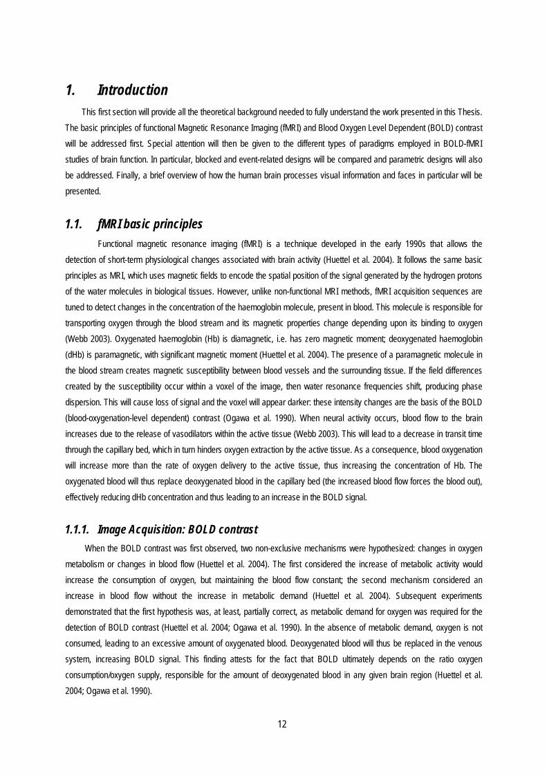
FIGURE 1: HEMODYNAMIC RESPONSE FUNCTION (HRF) FOR A HYPOTHETICAL SHORT-DURATION STIMULUS, REPRESENTED BY THE RED BAR. BOLD RESPONSE FIRST DESCRIBES A DIP, ALSO KNOWN AS THE INITIAL DIP, REACHING ITS PEAK AT APPROXIMATELY 5S. AFTERWARDS, MR (MAGNETIC RESONANCE) SIGNAL DECREASES UNTIL IT REACHES A VALUE LOWER THAN THAT OF BASELINE – UNDERSHOOT. SIGNAL THEN RETURNS TO BASELINE (AMARO AND BARKER 2006). 14

FIGURE 2: LINEARITY IN HEMODYNAMIC RESPONSE. IF TWO CONSECUTIVE STIMULI ELICIT THE EXACT SAME RESPONSE, THEN HDR WOULD BE A LINEAR COMBINATION OF BOTH (A AND B). HOWEVER, IF THE SUCCESSION IN WHICH THE STIMULI OCCUR IS TOO FAST , THEN THE COMBINED RESPONSE WILL EXHIBIT A DECREASE IN AMPLITUDE (C AND D) (HUETTEL ET AL. 2004). 14

FIGURE 3: BASIC PRINCIPLES OF GLM. DESIGN MATRIX IS DEFINED BY THE USER ACCORDING TO THE

GOALS OF THE EXPERIMENT. THE MODEL WILL TRY TO DEFINE THE PARAMETERS OF THAT

BETTER DESCRIBE , FOR A MINIMUM VALUE OF (HUETTEL ET AL. 2004). 15

FIGURE 4: THREE MAIN REGIONS FOR FACE PROCESSING IN THE BRAIN. BOTH LATERAL (ABOVE) AND VENTRAL (BELOW) VIEWS ARE SHOWN. FSTS STANDS FOR “FACE STS” (KANWISHER AND YOVEL 2006). 22

FIGURE 5: EXAMPLE OF A FACE SET. 25

FIGURE 6: EXAMPLE OF A FACE ROTATED IN ALL 6 ORIENTATIONS (RESPECTIVELY 0°, 60°, 120°, 180°, 240° AND 300°). 26

FIGURE 7: TWO FACES AND THEIR RESPECTIVE MASKS. THE EFFECT OF DIFFERENT HAIR COLOURS IS VISIBLE, AS THE MASK ON THE RIGHT IS DARKER THAN THE ONE ON THE LEFT. 26

FIGURE 8: TRIAL STRUCTURE DIAGRAM. 27

FIGURE 9: BLOCK DESIGN PARADIGM DIAGRAM. 6 CONSECUTIVE BLOCKS OF STIMULI ARE FOLLOWED BY A FIXATION BLOCK, OF THE SAME LENGTH. THIS PATTERN IS REPEATED 6 TIMES THROUGHOUT THE PARADIGM, WITH THE ORIENTATION ORDER CHANGING EACH TIME. THE ORIENTATION ORDER SHOWN CORRESPONDS TO THE FIRST 6 BLOCKS. 28

FIGURE 10: EXAMPLE OF AN EVENT-RELATED DESIGN DIAGRAM. RED LINES REPRESENT FIXATION TRIALS; THE REMAINING LINES REPRESENT TASK TRIALS: EACH COLOUR IDENTIFIES A DIFFERENT STIMULI LEVEL. NOTICE THAT THE DISTANCE BETWEEN EACH BAR IS NOT UNIFORM, INDICATING THE PRESENCE OF JITTER. THE RATIO (TASK TRIALS)/(FIXATION TRIALS) IS NOT THE SAME AS WAS USED IN THE CURRENT PARADIGM. [BASED ON A FIGURE IN (MECHELLI ET AL. 2003)] 29

FIGURE 11: EXAMPLE OF A PARAMETRIC DESIGN DIAGRAM. THE PARAMETER IN QUESTION IS BLOCK, WHICH IS THE PARAMETER CONSIDERED FOR THE LEARNING PARADIGM. EACH BLOCK CONTAINS

8

A NUMBER OF TRIALS (6 IN THE CASE OF LEARNING), OCCURRING IN SUCCESSION. IN OTHER WORDS, THE FIRST BLOCK CONTAINS THE FIRST 6 TRIALS, THE SECOND TRIALS 7 TO 12, AND SO ON. FOR LEARNING, AS FOR FR-BD AND FR-ER, TOTAL NUMBER OF BLOCKS IS 36. 29

FIGURE 12: BLOCK ORDER FOR RUNS 1 AND 3 (ABOVE) AND RUNS 2 AND 4 (BELOW). NOTE THAT THE LAST 2 SETS OF BLOCKS OF ONE RUN ARE THE FIRST 2 SETS OF THE OTHER RUN. “DUMMIES” CORRESPOND TO THE INITIAL FIXATION PERIOD. FIXATION BLOCKS ARE IDENTIFIED AS BASELINE. 30

FIGURE 13: GUIDE USER INTERFACE (GUI) DESIGNED FOR THIS STUDY. THIS INTERFACE IS DIVIDED INTO THREE SECTIONS, ONE FOR ANALYSIS AND ONE FOR CHART-BUILDING. A THIRD SECTION WAS INCLUDED TO SHOW A PREVIEW OF THE OVERALL RESULTS OF A GIVEN ANALYSIS; CURRENTLY, THE RESULTS SHOWN ARE FOR FR – ER. ALL THE INFORMATION REQUIRED FOR THE PROCESSING OF DATA IS INTERACTIVELY ASKED THE USER IN THE COURSE OF THE RESPECTIVE PROGRAM. 31

FIGURE 14: GROUP RESULTS OF FR-BD: A) RESPONSE TIMES AS FUNCTION OF BLOCK; B) ERROR RATES AS A FUNCTION OF BLOCK; C) RESPONSE TIMES AS A FUNCTION OF ORIENTATION; D) ERROR RATES AS A FUNCTION OF ORIENTATION. BARS REPRESENT AVERAGES OVER ALL SUBJECTS AND ERROR BARS REPRESENT THE STANDARD ERROR OF THE MEAN. ORIENTATIONS 1-6 CORRESPOND RESPECTIVELY TO 0°, 60°, 120°, 180°, 240°AND 300°. 37

FIGURE 15: EXAMPLES OF SINGLE-SUBJECT RESULTS OF FR-BD: A) RESPONSE TIMES AS FUNCTION OF BLOCK; B) ERROR RATES AS A FUNCTION OF BLOCK; C) RESPONSE TIMES AS A FUNCTION OF ORIENTATION; D) ERROR RATES AS A FUNCTION OF ORIENTATION. BARS REPRESENT AVERAGES OVER ALL SUBJECTS AND ERROR BARS REPRESENT THE STANDARD ERROR OF THE MEAN. ORIENTATIONS 1-6 CORRESPOND RESPECTIVELY TO 0°, 60°, 120°, 180°, 240°AND 300 °. 38

FIGURE 16: GROUP RESULTS OF FR-ER: A) RESPONSE TIMES AS FUNCTION OF BLOCK; B) ERROR RATES AS A FUNCTION OF BLOCK; C) RESPONSE TIMES AS A FUNCTION OF ORIENTATION; D) ERROR RATES AS A FUNCTION OF ORIENTATION. BARS REPRESENT AVERAGES OVER ALL SUBJECTS AND ERROR BARS REPRESENT THE STANDARD ERROR OF THE MEAN. ORIENTATIONS 1-6 CORRESPOND RESPECTIVELY TO 0°, 60°, 120°, 180°, 240°AND 300°. 40

FIGURE 17: EXAMPLES OF SINGLE-SUBJECT RESULTS OF FR-ER: A) RESPONSE TIMES AS FUNCTION OF BLOCK; B) ERROR RATES AS A FUNCTION OF BLOCK; C) RESPONSE TIMES AS A FUNCTION OF ORIENTATION; D) ERROR RATES AS A FUNCTION OF ORIENTATION. BARS REPRESENT AVERAGES OVER ALL SUBJECTS AND ERROR BARS REPRESENT THE STANDARD ERROR OF THE MEAN. ORIENTATIONS 1-6 CORRESPOND RESPECTIVELY TO 0°, 60°, 120°, 180°, 240°AND 300 °. 41

FIGURE 18: GROUP RESULTS OF THE LEARNING EXPERIMENT: ERROR RATES (TOP) AND RESPONSE TIMES (BOTTOM), AS A FUNCTION OF SESSION (LEFT), BLOCK FOR TRAINING PHASE (MIDDLE) AND BLOCK FOR TRANSFER PHASE (RIGHT). BARS REPRESENT AVERAGES OVER ALL SUBJECTS AND ERROR BARS REPRESENT THE STANDARD ERROR OF THE MEAN. SESSION 5 CORRESPONDS TO TRANSFER SESSION. 42

9

FIGURE 19: EXAMPLES OF SINGLE-SUBJECT RESULTS OF LEARNING PARADIGM, TRAINING PHASE (TOP) AND TRANSFER PHASE (BOTTOM). BARS REPRESENT VALUES OF BLOCK AND ERROR BARS REPRESENT THE STANDARD ERROR OF THE MEAN. 43

FIGURE 20: REPRESENTATIVE EXAMPLES OF SINGLE-SUBJECT RESULTS OF LEARNING PARADIGM: A) RESPONSE TIMES AS FUNCTION OF SESSION B) ERROR RATES AS A FUNCTION OF SESSION. BARS REPRESENT AVERAGES OVER ALL BLOCKS AND ERROR BARS REPRESENT THE STANDARD ERROR OF MEAN. SESSION 5 CORRESPONDS TO TRANSFER PHASE. 44

FIGURE 21: DESIGN MATRIX FOR LOCA. TIME IS DISPLAYED VERTICALLY AND EACH COLUMN CORRESPONDS TO AN EV. CONTRASTS ARE SHOWN IN THE BOTTOM AND IDENTIFIED AS C1-C10. THE TWO RIGHTMOST COLUMNS PERTAIN TO THE EV “SCRAMBLED (OBJECTS)”; THE BAD DISPLAY IS A CONSEQUENCE OF WORD LENGTH. 45

FIGURE 22: RESULTS FOR LOCALISER, DISPLAYED IN CORONAL (LEFT) AND TRANSVERSAL (RIGHT) PLANES. THE RELEVANT CLUSTERS OF THE STATISTICAL Z MAPS ARE SHOWN OVERLAID ON THE MNI TEMPLATE IMAGE (RIGHT HEMISPHERE IS ON THE LEFT). (A) ACTIVATION MAP FOR O>S (2.3<Z<13.3), SHOWING THE LOC BILATERALLY. (B) ACTIVATION MAP FOR H>S (2.3<Z<11.0), SHOWING THE PPA BILATERALLY. (C) ACTIVATION FOR F>S (2.3<Z<9.6), SHOWING THE LOC, PREDOMINANTLY ON THE RIGHT HEMISPHERE (ACTIVATION WAS REGISTERED BILATERALLY); (D) ACTIVATION FOR F>S, (2.3<Z<9.3), SHOWING THE FFA, ON THE RIGHT HEMISPHERE. 46

FIGURE 23: OVERALL RESULTS FOR LOCALISER, DISPLAYED IN CORONAL (LEFT) AND TRANSVERSAL (RIGHT) PLANES. CONTRASTS FOR FACES (RED), HOUSES (BLUE) AND OBJECTS (GREEN) ARE OVERLAID ON THE MNI TEMPLATE AND RIGHT HEMISPHERE IS ON THE LEFT.. MNI COORDINATES OF SLICES ARE: Y=-74 (CORONAL) AND Z=-6 (TRANSVERSAL). 46

FIGURE 24: DESIGN MATRICES FOR FR-BD (TOP) AND FR-ER (BOTTOM). TIME IS DISPLAYED VERTICALLY AND EACH COLUMN CORRESPONDS TO AN EV. CONTRASTS ARE SHOWN IN THE BOTTOM AND IDENTIFIED AS C1-C13. 47

FIGURE 25: MOTION CHARTS FOR BD, SESSION 1. ESTIMATED VALUES FOR ROTATIONS (TOP), TRANSLATIONS (MIDDLE) AND MEAN DISPLACEMENTS (BOTTOM) ARE SHOWN FOR ALL VOLUMES COLLECTED. ABSOLUTE MEAN DISPLACEMENT WAS 1.95 MM; RELATIVE MEAN DISPLACEMENT WAS 0.14 MM CHARTS OBTAINED FROM FSL PRE-STATS (JENKINSON ET AL. 2002; SMITH 2002). 48

FIGURE 26: RESULTS FOR BLOCK DESIGN: QUADRATIC CONTRAST (RED, 3.5<Z<8.9) OVERLAID ON THE LOCALISER CONTRAST FOR FACES (BLUE, 3<Z<9.3). RIGHT HEMISPHERE IS ON THE LEFT. BACKGROUND IMAGE IS MNI TEMPLATE. TOP LEFT IMAGE CORRESPONDS TO SLICE Z=-24; BOTTOM RIGHT IMAGE CORRESPONDS TO SLICE Z= 22 .PURPLE AREAS INDICATE OVERLAP OF THE QUADRATIC EFFECT ON FACE PROCESSING AREAS. OVERLAP WAS DETECTED FOR LOC AND FFA, IN BOTH HEMISPHERES.. 49

10

FIGURE 27: RESULTS FOR EVENT RELATED DESIGN: QUADRATIC CONTRAST (RED, 2.3<Z<5.3) OVERLAID ON THE LOCALISER CONTRAST FOR FACES (BLUE, 3.0<Z<9.3). RIGHT HEMISPHERE IS ON THE LEFT. BACKGROUND IMAGE IS MNI TEMPLATE. TOP LEFT IMAGE CORRESPONDS TO SLICE Z=-24; BOTTOM RIGHT IMAGE CORRESPONDS TO SLICE Z= 22 .PURPLE AREAS INDICATE OVERLAP OF RESULTS. OVERLAP WAS DETECTED FOR LOC. 50

FIGURE 28: EXAMPLE OF GIBBS RINGING OBTAINED FOR RUN 2 OF FR-ER. 51

List of Tables

TABLE 1: FMRI PARAMETERS USED IN THE DIFFERENT ACQUISITIONS PERFORMED IN THE PILOT

EXPERIMENT ................................................................................................................................................................. 34

11

List of Abbreviations BD – Block Design

BOLD – Blood Oxygen Level Dependent

CBF – Cerebral Blood Flow

CMRO2 - Cerebral Metabolic Rate for Oxygen

COG – Centre of Gravity

CRMglu - Cerebral Metabolic Rate for Glucose

dHb – deoxygenated haemoglobin

EEG – Electroencephalogram

ER – Event Related

ERP – Event-related Potential

EV – Explanatory variable

F – Faces

FFA – Fusiform Face Area

FIE – Face Inversion Effect

fMRI – functional Magnetic Resonance Imaging

FOV – Field of View

FR – Face Rotation

FR-BD - Face Rotation-Block Design

FR-ER - Face Rotation-Event Related Design

GLM – General Linear Model

GUI – Guide User Interface

H – Houses

Hb – Haemoglobin

HRF – Hemodynamic Response Function

ISI – Interstimulus Interval

IV – Independent variable

LOC – Lateral Occipital Complex

LOCA - FFA-PPA-LOC Localiser

MR - Magnetic Resonance

MRI – Magnetic Resonance Imaging

O – Objects

OFA – Occipital Face Area

PET – Positron Emission Tomography

PPA – Parahippocampal Place Area

S – Scrambled Objects

SNR – signal to noise ratio

STS – Superior Temporal Sulcus

MNI – Montreal Neurological Institute

12

1. Introduction This first section will provide all the theoretical background needed to fully understand the work presented in this Thesis.

The basic principles of functional Magnetic Resonance Imaging (fMRI) and Blood Oxygen Level Dependent (BOLD) contrast will be addressed first. Special attention will then be given to the different types of paradigms employed in BOLD-fMRI studies of brain function. In particular, blocked and event-related designs will be compared and parametric designs will also be addressed. Finally, a brief overview of how the human brain processes visual information and faces in particular will be presented.

1.1. fMRI basic principles Functional magnetic resonance imaging (fMRI) is a technique developed in the early 1990s that allows the

detection of short-term physiological changes associated with brain activity (Huettel et al. 2004). It follows the same basic principles as MRI, which uses magnetic fields to encode the spatial position of the signal generated by the hydrogen protons of the water molecules in biological tissues. However, unlike non-functional MRI methods, fMRI acquisition sequences are tuned to detect changes in the concentration of the haemoglobin molecule, present in blood. This molecule is responsible for transporting oxygen through the blood stream and its magnetic properties change depending upon its binding to oxygen (Webb 2003). Oxygenated haemoglobin (Hb) is diamagnetic, i.e. has zero magnetic moment; deoxygenated haemoglobin (dHb) is paramagnetic, with significant magnetic moment (Huettel et al. 2004). The presence of a paramagnetic molecule in the blood stream creates magnetic susceptibility between blood vessels and the surrounding tissue. If the field differences created by the susceptibility occur within a voxel of the image, then water resonance frequencies shift, producing phase dispersion. This will cause loss of signal and the voxel will appear darker: these intensity changes are the basis of the BOLD (blood-oxygenation-level dependent) contrast (Ogawa et al. 1990). When neural activity occurs, blood flow to the brain increases due to the release of vasodilators within the active tissue (Webb 2003). This will lead to a decrease in transit time through the capillary bed, which in turn hinders oxygen extraction by the active tissue. As a consequence, blood oxygenation will increase more than the rate of oxygen delivery to the active tissue, thus increasing the concentration of Hb. The oxygenated blood will thus replace deoxygenated blood in the capillary bed (the increased blood flow forces the blood out), effectively reducing dHb concentration and thus leading to an increase in the BOLD signal.

1.1.1. Image Acquisition: BOLD contrast When the BOLD contrast was first observed, two non-exclusive mechanisms were hypothesized: changes in oxygen

metabolism or changes in blood flow (Huettel et al. 2004). The first considered the increase of metabolic activity would increase the consumption of oxygen, but maintaining the blood flow constant; the second mechanism considered an increase in blood flow without the increase in metabolic demand (Huettel et al. 2004). Subsequent experiments demonstrated that the first hypothesis was, at least, partially correct, as metabolic demand for oxygen was required for the detection of BOLD contrast (Huettel et al. 2004; Ogawa et al. 1990). In the absence of metabolic demand, oxygen is not consumed, leading to an excessive amount of oxygenated blood. Deoxygenated blood will thus be replaced in the venous system, increasing BOLD signal. This finding attests for the fact that BOLD ultimately depends on the ratio oxygen consumption/oxygen supply, responsible for the amount of deoxygenated blood in any given brain region (Huettel et al. 2004; Ogawa et al. 1990).

13

Determining oxygen consumption, is not, however, a straightforward task, as the relation between neural activity and oxygen consumption hinges on other physiological factors, such as the glucose metabolism. While cerebral blood flow (CBF) and the cerebral metabolic rate for glucose (CRMglu) increase at a similar rate in the presence of a visual stimulus, the cerebral metabolic rate for oxygen (CMRO2) increases in a much slower fashion, which provides evidence of an uncoupling between oxygen and glucose uptake (Huettel et al. 2004). One possible explanation for this may be the need for an excess in oxygen supply, so as to compensate for the inefficiencies of diffusion when blood velocity is high. Alternatively, this mismatch could also be due to the vasculature delivering a fixed ratio of oxygen and glucose, appropriate for an aerobic process: if part of the glucose is converted via an anaerobic process, there will be an oxygen surplus (Logothetis and Wandell 2004). This model thus considers anaerobic metabolism to be negligible, contradicting the first hypotheses (Logothetis and Wandell 2004).

There isn’t a definitive explanation for the interaction of blood flow and glucose. The initial dip, a decrease in MR signal prior to positive signal change, is partially responsible for this. Its existence is attributed to a (transient) increase in dHb (Amaro and Barker 2006), but this is somewhat controversial (Huettel et al. 2004). A recent model, the balloon model, (Huettel et al. 2004), proposes that the increase of inflow to the venous system far surpasses the outflow, thus the system expands like a balloon to accommodate it. This would mean that rather than disappearing from the venous system, dHb would linger for some time, causing small veins to be mostly dominated by it, leading to the signal decrease. If this model is correct, it would mean that the initial dip is not a good spatial indicator of neural activity, since blood flow is coarse and not localized. Therefore, this effect would be detected throughout the brain, not only in the active areas, which could pose as a danger in interpreting fMRI results and the BOLD hemodynamic response (Huettel et al. 2004).

The time course of the hemodynamic response to an instantaneous pulse of stimuli-triggered neuronal activity is described by the hemodynamic response function (HRF) (Logothetis and Wandell 2004). This may vary in shape according to the stimuli presented, the neuronal process elicited and even the active area. Although it is difficult to predict the exact shape of the HRF, it is expected to be related with the rate of neuronal firing. Additionally, it has been observed that the HRF lags behind neuronal activity, which happens within milliseconds of stimulus presentation, taking up to a few seconds to occur (Huettel et al. 2004; Logothetis and Wandell 2004). Regardless of all the possible differences, the HRF usually follows a basic shape, beginning with an initial dip (consequence of a temporary increase in deoxyhaemoglobin, due to the delay of the inflow of oxygenated blood needed to suppress metabolic needs). As more oxygenated blood flows into the brain, deoxygenated brain is flushed out, and the signal increases to a peak, usually at approximately 5 s (Huettel et al. 2004). This increase is proportional to the underlying neural activity. If this is extended over a block of (sufficient) time, a plateau is reached, instead of peak (Amaro and Barker 2006), usually at 6-9 s (Logothetis and Wandell 2004). After this, a decrease occurs, originating a post-stimulus undershoot, due to the different decreasing rates of blood flow and blood volume: as blood flow changes more rapidly, dHb increases, since the inflow of Hb is severely reduced, and the signal decreases, making the overall signal inferior to baseline (Huettel et al. 2004). The basic shape of the HRF is represented in Figure 1.

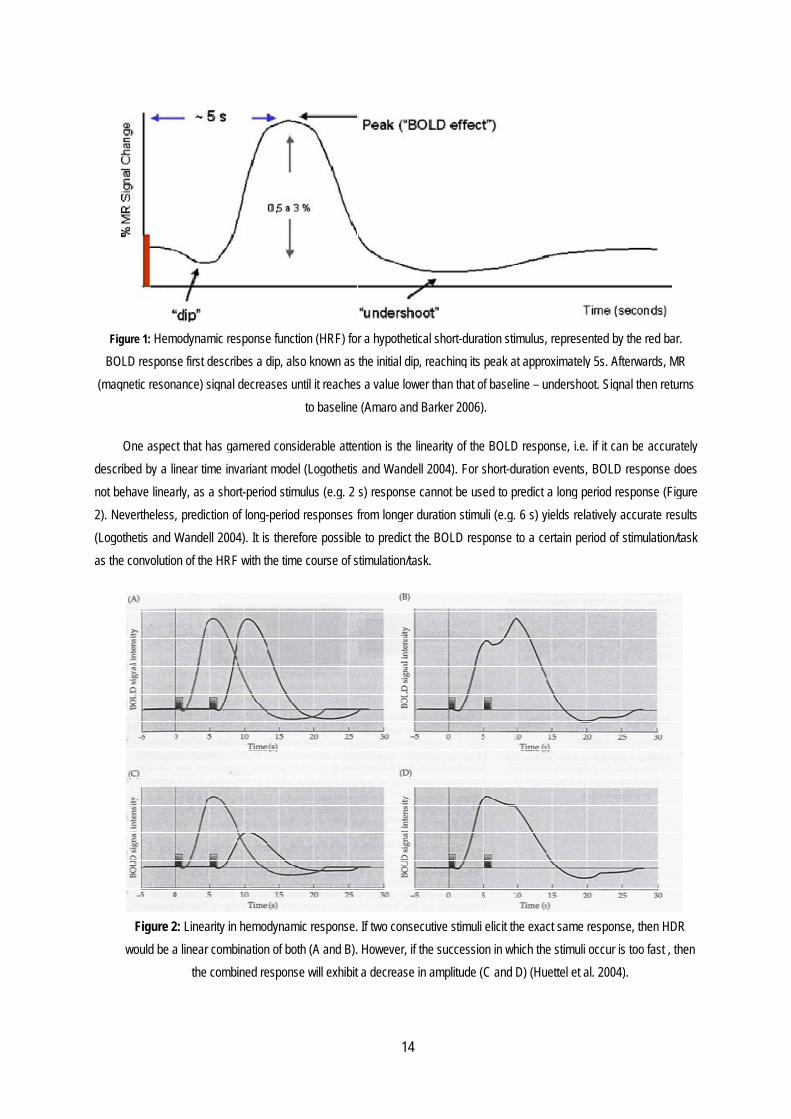
Figure 1

BOLD re(magnetic

Onedescribed not behav2). Nevert(Logothetias the con

Fiwou

1: Hemodynamesponse first dec resonance) sig

aspect that ha by a linear time linearly, as a heless, predicts and Wandell

nvolution of the

igure 2: Linearuld be a linear c

the c

mic response funescribes a dip, gnal decreases

as garnered conme invariant mod

short-period stion of long-peri 2004). It is the HRF with the ti

ity in hemodynacombination of bcombined respo

nction (HRF) foalso known as

s until it reachesto baseline

nsiderable attedel (Logothetistimulus (e.g. 2 iod responses ferefore possibleime course of s

amic response.both (A and B).

onse will exhibit

14

r a hypotheticathe initial dip, rs a value lower (Amaro and Ba

ntion is the lines and Wandell 2s) response cafrom longer due to predict thestimulation/task

If two consecu However, if the

t a decrease in

l short-durationeaching its pea than that of baarker 2006).

earity of the BO2004). For shorannot be used tration stimuli (e

e BOLD respon.

utive stimuli elice succession inamplitude (C a

n stimulus, repreak at approximaaseline – unders

OLD response, rt-duration evento predict a longe.g. 6 s) yields se to a certain

cit the exact samn which the stimnd D) (Huettel e

esented by the ately 5s. Afterwashoot. Signal th

i.e. if it can bents, BOLD respg period responrelatively accu period of stimu

me response, thmuli occur is tooet al. 2004).

red bar. ards, MR hen returns

accurately ponse does nse (Figure rate results ulation/task

hen HDR o fast , then

1.1.2. DThe a

the stimuluby:

where i

remain co

of each m

be relevan

combinatioaccommod

This eis represebecause estructure.

be used).

parameteris of dimen(Figure 3).

Figure mod

Tvalues for The signifi

Data Analyanalysis of fMRus/task of intere

s the observed

nstant during t

odel factor ,

nt; thus, the o

on of coefficiedate multiple va

equation translented by a matrerror and para

is the design

As each of th

r matrix, , mannsions: M mod.

3: Basic princip

del will try to def

The model is a each voxel wilicance of the m

ysis: GeneraRI data is aimed est. For this pur

d response, is

he experiment.

according to th

nly known dat

ents that mariables a new e

ates the basic rix , of N timemeter weight v

n matrix, which

ese factors cor

nages the relatiel factors x V v

ples of GLM. De

fine the parame

adjusted to thel be obtained b

model is then tes

al Linear M at detecting thrpose, fMRI dat

s an additive e

. The remaining

heir influence in

ta is . Howev

minimize (whiequation emerg

principles of the points by V vvalues are calcspecifies the m

rresponds to a

ive (weighted) cvoxel; thus, eac

esign matrix

eters of that b

e data in ordby combining alsted for each v

15

Model (GLM)e brain regionsta may be expre

error term and

g coefficient

n . Model fact

ver, with a give

ch is then knges:

e GLM in fMRIvoxels (re-arranculated indepe

model to be used

a column, is o

contributions ofch cell of this m

is defined by th

better describe

der to obtain thll time points, i.

voxel, usually by

) where the BOLessed by a gen

the term re

ts are paramete

ors are hypothe

en set of mode

own as the r

I. In this model,nged in one dindently for all d (in terms of de

of dimensions:

f each regressomatrix indicates

he user accordi

, for a minimu

he combinatione. by using a cy dividing the a

LD signal time cneral linear mod

epresents the c

er weights, rep

esized compon

el factors it is

esidual). If Eq

, experimental mension, for si voxels, withouesign factors an

N time points

or present in tparameter amp

ng to the goals

um value of (

of weights thacost function, usmplitude of the

course is correldel (GLM), as de

contribution of f

presenting the c

nents of the dat

possible to es

quation 1 is a

data (observedimplicity). This ut regard for fMnd confounds th

x M model fac

to response ; plitude for a sp

of the experim

(Huettel et al. 2

at minimizes sually least-squ

e considered pa

lated with escribed

(1)

factors that

contribution

ta that may

stimate the

arranged to

(2)

d response) is possible

MRI spatial hat need to

ctors. The

as such, ecific voxel

ment. The

004).

. The error uares error. arameter by

16

the residual error (in a given voxel). As this quantity should follow the F-distribution, as per the null hypothesis, it is thus possible to evaluate its significance by a degrees of freedom method (Friston 2005).

Besides the BOLD response prediction, other factors may be added to . Three types of factors are considered: covariates, indicators and nuisance factors. Covariates are factors that may take any of a continuous range of values (predicted BOLD signal is the most common factor in this category), while nuisance factors include non-experimental known sources of variability (such as scanner drift or motion parameters); indicators are qualitative factors, hence only taking integral values - 0 or 1, depending upon whether the corresponding experimental factor is absent or present (Friston 2005). Adding these extra factors helps to ensure the error residuals have the expected Gaussian random distribution, each being independent and identically distributed: it is therefore advisable to include all known sources of variation in the model. However, introducing an excessive number of factors is undesirable, as each will reduce the number of degrees of freedom by one, creating a more conservative statistical model, albeit more valid. The inclusion of correlated factors on the other hand, must be avoided at all costs, as it could pollute the data: if two factors are related, variance attributed to one of them, might in fact be caused by being correlated with another factor. Moreover, can also be modified to include the interaction effects between BOLD and other sources of variance, such as motion parameters.

The GLM is a powerful tool for analyzing fMRI data, but it relies on a number of assumptions. The most important of these assumptions is the use of a standard HRF function, usually a gamma function (Huettel et al. 2004). However in more complex situations, it could be sometimes useful to divide the BOLD response into phases, to obtain a better prediction, according to the processes evoked by the task. Inclusion of additional factors to model small differences in the onset of the HRF, such as time derivatives, is also frequently used. It has been shown that subject specific HRFs help to overcome the effects of inter-subject variability; these HRFs would be obtained from a previous fMRI experiment. Another assumption is linearity. While it is true that the BOLD response is not linear at short stimulus intervals, provided that long enough stimuli are used, then the overall time course is guaranteed to be linear and thus the HRF can be linearly added in the form of a convolution. A third assumption pertains to the use of the same HRF for each subject throughout the brain, as it has been shown to vary, especially in latency. Fitting the model in order to determine the HRF using a combination of basis functions (such as sines, co-sines and gamma functions) would be a way to overcome this problem, by introducing some flexibility into the model. Additionally, voxels are assumed to be independent, even adjacent ones, which is obviously not generally true. This can be overcome by introducing a known correlation factor between such voxels, using spatial smoothing procedures during pre-processing. The individual time points are also assumed to vary independently but certain factors, such as scanner drift, can introduce considerable variability across time points. This may not always actually happen, mostly due to differences in noise during activity (higher) and rest (lower) (Huettel et al. 2004).

1.2. fMRI design The GLM can be used in different ways, depending on the goal of the analysis to be performed (Friston 2005). The

most relevant parameters for any fMRI experiment are detection and estimation. The first pertains to identifying active voxels and the latter to knowing the time course of the activated voxels. Since detection and estimation depend on different factors – respectively on the total variance of BOLD signal and on stimulus randomness – it might not be possible to create an fMRI design that enables simultaneously good detection and good estimation (Huettel et al. 2004). Two main types of stimulation/task paradigm designs can be employed: Event-Related (ER) and Blocked (BD) designs. They will be separately

17

described next. A particular type of designs will also be described – parametric designs, which aim at analysing the parametric effects of specific factors, such as learning with practice.

1.2.1. Blocked Designs (BD) Blocked designs (BD) are characterized by grouping together stimuli with the same level of the independent

variable (stimulus category / task condition) which remains constant throughout the block (Huettel et al. 2004). This is a fairly simple design to create, and its analysis it’s also straightforward: the dependent variable in each block may be directly compared with the remaining blocks. Additionally, this design also allows for a continued stimulation, as cognitive engagement is sustained throughout the epochs, period of time during which a given level is shown (Amaro and Barker 2006). However, blocks still need to obey certain constrains. They must be suited to the research question itself: while in some experiments longer task blocks are advantageous, i.e. if attention is required (active concentration requires some time to engage), block use is undesired in others, such as those that only elicit transient responses (Huettel et al. 2004). Additionally, blocks must also have an appropriate length; “appropriate” in this case pertains to the dependent variable, since block timing is adjusted to match the hemodynamic response function expected. Each block must also be assigned a set of (experimental) conditions, namely concerning the level of the IV (independent variable).

The way blocks are presented (alternating conditions, for instance) also needs to be taken into account. Using the alternating design will allow for comparison between two (or more) conditions, but will not give any information regarding the differences between rest and activation states. To enable this comparison, another design is necessary using control or null-task blocks, which are a particular kind of control blocks where the subject is passive. This introduces a resting state condition and allows for comparisons not only between states, but also between rest and activation. Comparing between individual blocks and the rest state is also possible, depending largely on the goals of the experiment. Increasing the number of conditions (not only by including null-trials, but also by raising IV levels) will obviously increase the number of comparisons that can be made, resulting in more information. In any case, it should be noted that each additional condition is time consuming and should be avoided if not extremely necessary. (Huettel et al. 2004)

Timing the blocks is also an important aspect of design setup, depending mostly on the experiment to be conducted and on eventual time constraints. For instance, in the case of memory experiences, the size of the blocks may influence the difficulty of the experiment. On the other hand, factors like fatigue and practice should also be accounted for when establishing the duration of each block, as these interfere with mental processes and may falsify the results. Regardless of the duration chosen, block length should remain constant across all conditions, including control conditions; this is a necessary step so that each block has the same statistical validity. Comparing blocks with different lengths (which translates into different number of observations/trials per block) will decrease the experiment’s statistical power, as length influences the standard deviation of each data set. (Huettel et al. 2004)

Advantages and disadvantages of blocked designs Blocked designs are simple designs, as it has been established, but they can also be very powerful. Generally

speaking, blocked designs have a good capability of detecting relevant fMRI activity, which comes from balancing two factors: difference in BOLD signals between conditions and number of transitions between conditions. The first factor is related to block length: if a block is longer than or equal to the hemodynamic response, then the response will be able to return to baseline, thus preserving its full amplitude; however, if the block length is inferior to the total duration of the

18

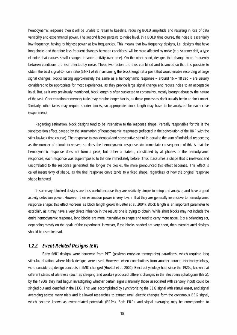
hemodynamic response then it will be unable to return to baseline, reducing BOLD amplitude and resulting in loss of data variability and experimental power. The second factor pertains to noise level. In a BOLD time course, the noise is essentially low frequency, having its highest power at low frequencies. This means that low frequency designs, i.e. designs that have long blocks and therefore less frequent changes between conditions, will be more affected by noise (e.g. scanner drift, a type of noise that causes small changes in voxel activity over time). On the other hand, designs that change more frequently between conditions are less affected by noise. These two factors are thus combined and balanced so that it is possible to obtain the best signal-to-noise ratio (SNR) while maintaining the block length at a point that would enable recording of large signal changes: blocks lasting approximately the same as a hemodynamic response – around 16 – 18 sec – are usually considered to be appropriate for most experiences, as they provide large signal change and reduce noise to an acceptable level. But, as it was previously mentioned, block length is often subjected to constraints, mostly brought about by the nature of the task. Concentration or memory tasks may require longer blocks, as these processes don’t usually begin at block onset. Similarly, other tasks may require shorter blocks, so appropriate block length may have to be analyzed for each case (experiment).

Regarding estimation, block designs tend to be insensitive to the response shape. Partially responsible for this is the superposition effect, caused by the summation of hemodynamic responses (reflected in the convolution of the HRF with the stimulus/task time course). The response to two identical and consecutive stimuli is equal to the sum of individual responses; as the number of stimuli increases, so does the hemodynamic response. An immediate consequence of this is that the hemodynamic response does not form a peak, but rather a plateau, constituted by all phases of the hemodynamic responses; each response was superimposed to the one immediately before .Thus it assumes a shape that is irrelevant and uncorrelated to the response generated; the longer the blocks, the more pronounced this effect becomes. This effect is called insensitivity of shape, as the final response curve tends to a fixed shape, regardless of how the original response shape behaved.

In summary, blocked designs are thus useful because they are relatively simple to setup and analyze, and have a good activity detection power. However, their estimation power is very low, in that they are generally insensitive to hemodynamic response shape: this effect worsens as block length grows (Huettel et al. 2004). Block length is an important parameter to establish, as it may have a very direct influence in the results one is trying to obtain. While short blocks may not include the entire hemodynamic response, long blocks are more insensitive to shape and tend to carry more noise. It is a balancing act, depending mostly on the goals of the experiment. However, if the blocks needed are very short, then event-related designs should be used instead.

1.2.2. Event-Related Designs (ER) Early fMRI designs were borrowed from PET (positron emission tomography) paradigms, which required long

stimulus duration, where block designs were used. However, when contributions from another source, electrophysiology, were considered, design concepts in fMRI changed (Huettel et al. 2004). Electrophysiology had, since the 1920s, known that different states of alertness (such as sleeping and awake) produced different changes in the electroencephalogram (EEG); by the 1960s they had begun investigating whether certain signals (namely those associated with sensory input) could be singled out and identified in the EEG. This was accomplished by synchronizing the EEG signal with stimuli onset, and signal averaging across many trials and it allowed researches to extract small electric changes form the continuous EEG signal, which became known as event-related potentials (ERPs). Both ERPs and signal averaging may be corresponded to

19

measures in the time series: ERPs correspond to epochs (fractions of a time series that are time-locked to a given event) and signal averaging corresponds to the averaged epoch (which is the averaging of all epochs pertaining to one condition; i.e. all stimuli with the same IV level).

As fMRI does not measure electrical activity of the brain, ERPs by themselves were not relevant to fMRI design; however, their underlying principles, time-locking and signal averaging, are independent of the type of signal measured, being valid both for electric and for hemodynamic measures, thus becoming the basic concepts for fMRI event-related (ER) design (Huettel et al. 2004). This design emerged in fMRI in the mid-90s, taking the advantage of the superior temporal resolution of fMRI when compared to PET. It is used when assuming that neural activity of interest would occur in short periods of time (transient activity), as the ability to detect such variations is main windfall of event-related designs (Amaro and Barker 2006). Stimuli that evoke such activity are known as trials or events. Unlike block design, in which each block corresponds to one level of the IV, in event-related design each event corresponds to one level of the IV. Additionally, instead of being presented in an alternating fashion, their order is (pseudo-)randomized. Another difference from blocked designs is that each pair of trials is separated by an interval, whereas in block design, trials may be presented in a continuous fashion. This interval can last as little as 2 s and as long as 20 s, depending on the experiment and its goals. The implementation of inter-stimulus intervals (ISI) reduces the predictability of the design, permitting a sustained attention level throughout the experiment (Amaro and Barker 2006).

Due to its characteristics, event-related designs brought a new perspective to fMRI analysis: while block designs concern steady-state activity at a given moment, event-related designs measure transient brain activity, so variation over time became the most important factor for analysing event related experiments. For this reason, this design requires a higher temporal resolution than blocked design, having consequences on both its detection and estimation capabilities. Generally speaking, event-related designs can be considered as impulses that generate a hemodynamic response. The amplitude and duration of this response will depend on the characteristics of the stimulus used (intensity and duration). Since trials work like impulses and the HRF has a linear behaviour for ISI values longer that 6 s, it should be possible to generate short stimuli and extract the HRF. In fact, it is possible to extract BOLD responses from closely spaced stimuli, provided that these are presented in a (pseudo-)random order. But small ISI values may not always be advisable: if the experiment aims at measuring the time course of the response or if baseline values are to be obtained, then longer intervals are more appropriate, in which the hemodynamic response has time to rise and fall to baseline. Particularly, the baseline is usually identified by averaging the time points that immediately precede stimulus onset; this is the equivalent to the null block in the blocked design, allowing for comparison between activated and rest states. However, the right size of the ISI may be difficult to establish.

But besides defining the length of the ISI, it is also important to define the fashion in which it occurs: they may be periodic (with constant duration) or jittered (the duration randomly varies between two preset values). Jittering, however, is not the same as randomizing: while the former pertains to the likelihood of a given interval following a given trial, the latter concerns itself with the likelihood of a trial being presented at a given time point. On the one hand, periodic design is simpler, although less effective: short intervals do not allow for the hemodynamic response to fully rise and fall, originating plateaus rather than peaks. There is a saturation of the BOLD signal, turning this design into a blocked design and thus eliminating any chance of individual trial analysis; longer intervals allow for a complete rise and fall of the hemodynamic response but have a low density of effects over time, which reduces detection power. Jittered interval durations prevent saturation of the

20

BOLD signal (because the ISI varies between stimuli) but these are only effective if they are sufficiently large when compared to the period of the hemodynamic response.

Advantages of Event-related designs Event-related designs mirror block designs. This is also true for strengths and weaknesses: these type of designs are

extremely good for estimating the shape of the HRF, but rather poor at detecting active voxels. In fact, estimation power is very important in most event-related experiments, as it allows the making of inferences regarding the timings of neural activities, feedback processes and sustained activity in a given region, all based on the timing and waveform of the hemodynamic responses. Additionally, event-related designs are also more flexible than blocked designs, allowing the separation of different brain processes associated with the same task and relating them to parts of the task. For example, since all fMRI experiments evoke multiple cognitive processes, using event-related experiments is a useful way of identifying and isolating the different cognitive processes associated with a given task. Another aspect of this flexibility derives from the fact that all trials occur individually, and not associated in blocks: this way, trials can be arranged and combined in the most convenient fashion, allowing for multiple comparisons using only one experimental run; this is often known as trial sorting (Huettel et al. 2004).

In summary, the extreme flexibility and high estimation power provided by event-related designs are its greatest strengths. This design is also less sensitive to head motion artifacts (Amaro and Barker 2006). However, these characteristics are counterbalanced the lack of detection power: using the wrong model of the HRF could invalidate a whole experiment, as the design could miss relevant voxels.

1.2.3. Parametric Designs Parametric designs are employed in order to study the effects of the modulation of a given stimuli, e.g., by creating

different levels of difficulty associated with a given task, but without changing the nature of the stimuli (Amaro and Barker 2006). In that case, the information about the relationship between the BOLD signal and a stimulus parameter (that may be either discrete or continuous) or a behavioural response may be extracted (Büchel et al. 1998). This would thus allow for the separation of the active brain areas of interest, the ones that respond to the modulation, from those that sustain baseline activation (Amaro and Barker 2006). However, this poses a difficulty, as defining a parameter that may be modulated and recruit only one type of cognitive processes could prove a difficult task. If this is not achieved, however, a “higher” (more difficult) level of the parameter will, in all likelihood, lead to activation of areas not directly correlated with it (Amaro and Barker 2006).

1.3. Face Processing Faces are highly relevant visual stimuli for humans. Through faces we are able to perceive the emotional state of an

individual, and choose the best course of action accordingly. As such, face processing is a vital skill for social interaction. It is thus unsurprising that face processing techniques and skills have been perfected in the course of evolution. It is now a highly specialized and complex process, so much that specific brain areas are more engaged in the processing of faces than other types of visual objects. In the following sections, those regions will be described. Additionally, a well known phenomenon of face processing will be analysed: the face inversion effect.

21

1.3.1. Face Inversion Effect The face inversion effect (FIE) was first reported in 1969, when Robert K. Yin found that inversion had a

disproportionate effect on face recognition (Rossion and Gauthier 2002). This raised awareness to how faces are handled by the brain, as it made investigators realize that face processing might follow its own methodology, individual from any other object. To this day, this topic still gathers great interest, partially fomented by developments in techniques – such as fMRI – that not only allow for a better view of the brain, but also enable to measure brain activity, at least to some extent. In fact, several studies have been conducted since 1969, focusing not only on faces but also on objects (cars, houses), animals (dogs, birds) and even on objects created specifically for that purpose (“Greebles”).

Causes for the FIE are not clear, and initial studies suggested that it could be a consequence of memory encoding of faces: processing was similar for upright and inverted faces, but encoding would be less efficient for inverted faces. This theory was later disproved, and there is now a growing consensus that FIE is independent from memory encoding. This seems to indicate that FIE occurs mainly during the primary encoding of faces, at a perceptual level (Rossion 2008). However, the face encoding process is, in itself, still a mystery, as there is no definitive evidence as to how faces are processed.

Although it has become clear that facial features are interdependent, there is no definitive evidence that a face is processed as a whole (holistically), or if features are processed simultaneously, in parallel or relationally (Rossion 2008). A recent study using composite face effect (the top and bottom halves of faces appear separately, creating the illusion that two top parts are different when the bottom part is), determined that brain activity is less susceptible to adaptation to faces when the top and bottom halves of a face are aligned than when they are misaligned. This seems to indicate that neurons use both parts to represent the whole of the face, thus proving the existence of holistic processing in the brain (Schiltz and Rossion 2006). It has also been discovered that the perception of metric distances is more affected by inversion than the perception of features themselves. In other words, FIE does not affect all facial cues in the same manner, which is why it is considered to alter face processing in a qualitative rather than a quantitative manner (Rossion 2008).

1.3.2. Effects of Learning It has been hypothesized that processing upright faces carries less error due to the fact that that is the way faces are

normally processed by our brain, i.e. because there has been a constant and continuous learning process (leading to expertise), and not because the brain might be unable to process them as accurately in any other orientation. However, the effects of processing faces presented at orientations other than 0° or 180° have not been studied extensively. In a 2007 study by Jacques and Rossion, 10 subjects were shown face photographs at 12 orientations (0°-360°, with 30° increments). Behavioural results showed that increasing orientation elicited higher response times and error rates, for orientations up to 120°. The interval 120° to 240° registered no significant increases in either variable. Orientations 240° to 360° yielded decreasing values for both variables (Jacques and Rossion 2007). A more recent study using only 6 orientations (0° to 300°, 60°increments), reported similar results for behavioural tests, although the highest response times and error rates values was reported for 180° rather than 120° (Gomes et al. 2009). Furthermore, this study also investigated the effect of a long-term training period (4 days, one session per day) on the processing of faces in multiple orientations. An improvement in the accuracy of face discrimination was found for a specific orientation (120º) that was neither 0° nor 180°. Additionally, this study also showed that, after the training period, the improvement in performance was also observed for the symmetric orientation (240º), suggesting that there was a transfer of learning across orientations.

22

1.3.3. Face regions in the brain Some regions of the brain specialize in a category of stimuli, i.e. respond more to a given category of stimuli, such as

places, objects or faces. Namely, a central complex of stimuli-selective activation in the lateral occipital cortex (LOC) (Grill-Spector and Malach 2004), has been reported to respond strongly to objects (Epstein et al. 2005; Grill-Spector and Malach 2004). One other region has been reported to respond more strongly to places and scenes than to other object categories (Peelen and Downing 2005); as such it is known as the parahippocampal place area or PPA (Grill-Spector and Malach 2004).

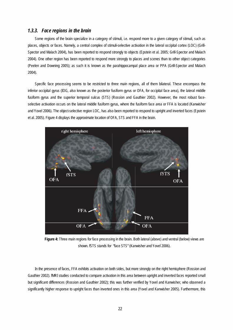
Specific face processing seems to be restricted to three main regions, all of them bilateral. These encompass the inferior occipital gyrus (IOG, also known as the posterior fusiform gyrus or OFA, for occipital face area), the lateral middle fusiform gyrus and the superior temporal sulcus (STS) (Rossion and Gauthier 2002). However, the most robust face-selective activation occurs on the lateral middle fusiform gyrus, where the fusiform face area or FFA is located (Kanwisher and Yovel 2006). The object-selective region LOC, has also been reported to respond to upright and inverted faces (Epstein et al. 2005). Figure 4 displays the approximate location of OFA, STS and FFA in the brain.

Figure 4: Three main regions for face processing in the brain. Both lateral (above) and ventral (below) views are

shown. fSTS stands for “face STS” (Kanwisher and Yovel 2006).

In the presence of faces, FFA exhibits activation on both sides, but more strongly on the right hemisphere (Rossion and Gauthier 2002). fMRI studies conducted to compare activation in this area between upright and inverted faces reported small but significant differences (Rossion and Gauthier 2002); this was further verified by Yovel and Kanwisher, who observed a significantly higher response to upright faces than inverted ones in this area (Yovel and Kanwisher 2005). Furthermore, this

23

study also showed that the FFA results were correlated with the behavioural face inversion effect (FIE), thus establishing the FFA as the source of the neural FIE. Nevertheless, the actual function of the FFA is not entirely clear.

It is possible that FFA may be more appropriate for detecting faces rather than processing them. This claim is based mainly on three findings: (i) Familiarity does not influence FFA activation. Additionally, it has also been suggested that, while the FFA may not be involved in maintaining long-term memories of faces, it may be responsible for the processing necessary to establish facial identity; (ii) the FFA shows only a moderate decrease in activation when comparing between the response to grayscale images and to line drawings of faces, despite this being a strategy that highly influences face perception; (iii) FIE for grayscale faces is small (Rossion and Gauthier 2002). These arguments, especially the latter two, seem to suggest that the FFA has the function of assessing whether the perceived object is a face rather that assessing whose face it is. However, older studies with prosopagnostic subjects show that lesions in face areas impair correct discrimination of faces, while face detection remains intact (Rossion and Gauthier 2002). Additionally, face processing, whether upright or inverted, seems to be highly dependent on expertise, as it has been demonstrated that autistic people show little evidence of the effects of expertise in faces, and in fact it has been suggested that they have no face expertise - poor eye contact is a known and characteristic manifestation of autism (Rossion and Gauthier 2002; Zwaigenbaum et al. 2005).

Another face region, the OFA (occipital face area), is thought to be involved in the initial phases of face processing and provides input to both STS and FFA. Its sensitivity to faces seems to be more focused on the right hemisphere (Rossion and Gauthier 2002). Regarding the FIE, this region shows higher activation for inverted than for upright faces or objects and inversion effects have been reported for both faces and Greebles (Rossion and Gauthier 2002). Greebles are novel objects, developed at Yale University by Scott Yu (http://titan.cog.brown.edu:8080/TarrLab/stimuli/novel-objects/greebles-2-0-symmetric.zip/view). They are hierarchically organized into genders, families and individuals, according to their characteristics. This creates the need of configural (holistic) processing to distinguish them, as the differences may be very subtle (Gauthier et al. 1998). This effect was not uniform in OFA, as some voxels showed a preference for inverted faces and Greebles, while others showed preference for upright Greebles. No voxels showed a preference for upright faces. This was later confirmed (Yovel and Kanwisher 2005), when it was observed that the OFA showed a similar response to both upright and inverted faces, thus showing no correlation with the neural FIE. Additionally, an effect of “familiarity” (to Greebles) was observed for this area; this should not be confused with the effect of expertise reported for FFA. Although the basic premise is the same, it occurs during a smaller span of time, a shorter training period. Therefore, expertise exhibits a correlation with behavioural changes occurring during its acquisition whereas familiarity is thought to occur as soon as subjects develop a canonical (base) orientation for a given category of objects.

The remaining face area, STS, also reported a significant decrease of activation for inverted faces, but only a non-significant one for object inversion. However, STS does not correlate with the neural FIE (Yovel and Kanwisher 2005). This finding supports the hypothesis that STS is responsible for processing the dynamic aspects of the face, such as gaze and expression rather than specialized in face identity (Yovel and Kanwisher 2005). This study also demonstrated that an object-selective region, the lateral occipital complex (LOC), also shows no correlation with the neural FIE, thus disproving an hypothesis that had been put forth by previous publications. However, it should be noted that, although it does not correlate with the neural FIE, this region does exhibit a larger activation for inverted than upright faces (Yovel and Kanwisher 2005). This is not entirely unexpected: as our exposure to faces is restricted to one orientation (upright) and, if face processing areas respond less to faces in other orientations, then it could be likewise expected that object processing areas would be

24

able to respond more to inverted faces (as these would be less perceived as faces) than to upright faces (Rossion and Gauthier 2002). However, inverted faces are not processed as regular objects, garnering more activation than non-face objects do in this area. This could be partially due to the fact that there is a phenomenon of transfer (at least to some extent) from upright objects to inverted ones, after training. In other words, the ability to better distinguish upright objects is partially maintained for inverted objects, although these were never trained. This effect was reported for Greebles, but the occurrence of such an effect for faces is not clear. It remains to be explained if training of a given orientation is the main cause of processing differences between faces in symmetrical orientations, or if the training process itself induces changes in the processing of the symmetrical orientation. For Greebles, a small difference was found between upright and inverted in novices, i.e. people with no experience in these objects. However, subsequent training caused the registered difference to increase, but only in the right-hemisphere FFA. Upright Greebles showed a correlation between these results and the increase in holistic processing during training was, but this was not verified for inverted Greebles or for faces, upright or inverted. These findings support the concept that expertise has an effect in FIE: as training progresses, processing strategies change and adapt, leading to a bigger effect of FIE (Rossion and Gauthier 2002).

1.4. Objectives The main objective of the work presented in this Thesis was the development of the methodological tools required for

the performance of a brain imaging experiment to study the mechanisms of face processing and learning in the human brain

using fMRI, basem d on the previous work in the group (Gomes et al., 2009). The specific aims of the project were:

1. To generate the stimuli: faces at multiples orientations. 2. To implement paradigms for both Event-Related and Block Designs of Face Rotation experiments, as well as for

Localizer and Learning experiments, using the software Presentation (Neurobehavioral Systems, http://www.neurobs.com/);

3. To implement data analysis code using MATLAB, for subsequent statistical analysis using SPSS; 4. To test the paradigms implemented here, by performing both behavioural and imaging experiments; 5. To compare the suitability of ER and blocked designs of the Face Rotation paradigms.

2. ImpT

steps invoexplains hthe previoorder to pwas improrelated deareas was

2.1. GeF

Biometrix of these sexternal feharmoniouconstructioversion: neeliminatingThere are were entirsuch as hexternal (hthat hair a

OIncorporatRGB scaleexpected corrected exactly for

plementinThis section ex

olved in the genhow the data anus work by Gorepare the prot

oved, the colousigns were imp

s also implemen

enerating tFaces to be use(www.iqbiomet

sets has one speature, there aus as possibleon of the sets oew features coug the need for usually at leasely alike. Desp

hair or eyes. Thair colour) andnd eye colour r

Once the facested). Here, the e). The gray baconsequence, for one face o

r all faces of ea

ng the Parxplains the metneration of the nalysis is execuomes et al. (Gotocols to be user and size wer

plemented to allnted.

the stimuli ed as stimuli wetrix.com/producpecific combinaare 3 sets of ie. Rare or noof internal featuuldn’t be starkly holistic processt two differenceite generating ghis was emplod internal (eye remained const

s were generate faces had the ackground wasreduce the am

of each set. Seach set. This wa

radigms thodology usedstimuli, while thuted. The stimuomes et al., 200ed in the fMRI re modified in oow improved se

i ere generated u

cts_faces_40.htation of externainternal featureticeable featurures was hindey different fromssing. Thus, intes between facgray scale imag

oyed in the crecolour) which want in each set

Figure 5

ed, they were e logo of IQ Bios used instead mount of baselieeing as this pras incompatible

25

d in this projeche second defiuli and paradigm09). However, experiments. Iorder to better ensitivity of the

using a demo vml). A total of 5al features (chies (Figure 5). res (such as eered by a narro

m the original onternal features

ces in a set, be ges, FACES4.0

eation of the fawere used to c of faces.

5: Example of a

exported to an iometrix removed

of a white oneine activation orocess was mae with the parad

ct and is subdivnes the paradigms implementespecific modificn particular, thesuit the fMRI s BOLD signal a

version of face c54 faces were gin, face shape,Feature distribextremely larg

ow array of chones, or the diffe vary not only it size, position

0 allowed for theaces, mostly to reate different

a face set.

mage editing sd and were ad

e in an attempt on primary visuanual, there wadigm being imp

vided into 3 pagms used. The

ed here were bacations and exe number and settings, block dand a localizer o

composite softwgenerated, grou, hair, ears andbution was thoe noses or e

oices, a conseqerence would be

in aspect but n, feature or a ce distinction of broaden the dfaces. It is imp

oftware, Photosded a gray bac to reduce imaual areas. Hairas an inherent plemented, as h

arts. The first ree third and last ased on the on

xtensions were quality of the sdesigns as welof the relevant v

ware, FACES 4uped in 18 setsd neck). For eaught out so as

eyes) were avoquence of usingecome extremealso in positioncombination; no shade in certadiversity of fea

portant to stress

shop 6.0 (Adobckground (135,

age brightness r contours weredifficulty in rep

having faces w

etraces the subsection

nes used in required in

stimuli used ll as event-visual brain

4.0, from IQ s of 3. Each ach type of s to be as oided. The g the demo ely obvious, n and size. o two faces in features,

atures, both s, however,

be Systems ,135,135 in and, as an e manually

producing it ith different

contours mresults. Tomake a tefaces. Onc0° throughnumber of

F

Fnoisy imagface is notimage conpixels fromverified byfaces witheach mask

Figure

2.2. DeF

SDL and P

1234

Epresented

might lead subjo overcome thisemplate from thce the faces weh 300°, every f faces generate

Figure 6: Exam

From the uprigges that result ft recognised asntaining the facm the backgrouy comparing mah darker hair geked had to be r

7: Two faces a

efining the Four different pPCL languages

1. Face Rota2. Face Rota3. Face Lear4. FFA-PPA-

Each of the fir sequentially a

ects to make ds difficulty, a sc

he outline of theere corrected th60° (6 orientated was thus 32

mple of a face ro

ht version of efrom the shufflis such. This effce and shuffles und is also incasks from faceenerate darker rotated in Photo

nd their respec

paradigmsparadigms were within the softw

ation – Block Deation – Event-Rerning: Training p-LOC Localiser

rst three paradand then the s

decisions basedcript was createe already correhey were exporttions, Figure 6)4.

otated in all 6 or

every face, a ming of the pixelsffect was obtain its pixels. Sinc

cluded in this ss with different masks (Figureoshop, in order

ctive masks. Thdarker t

s e implemented fware Presentat

esign (FR-BD) elated Design (phase + Transfe (LOCA)

digms consisteubject has to d

26

d on this and ned, using compcted face and ted back to Pho). Since each o

rientations (res

mask was geners in the face. Tned by creatingce the faces doshuffling, but it t hair colours: fe 7). As masks to obtain all the

e effect of diffethan the one on

for the study ofion.

(FR-ER) er phase(FL-Tr

d of a series decide whethe

not on the face puting software replace the inteotoshop to be rof the 54 faces

pectively 0°, 60

rated: each facThis way, the ovg a script in MAo not possess does not greafaces with light were built bas

e desired orient

rent hair colourn the left.

f face rotation a

rain + Trans)

of trials of a fr they are iden

itself as it is in MATLAB (fromernal features frotated into the s occurred in e

0°, 120°, 180°,

ce has its own verall image po

ATLAB; this scra regular geom

atly influence thter hair will gensed on the upritations.

rs is visible, as t

and associated

face discriminantical or differe

ntended, thus pm MathWorks). for those of the desired orientaeach orientatio

240° and 300°

specific mask. ower is maintainript selects a remetrical form, ahe outcome. Tnerate lighter might version of

the mask on th

learning effect

ation task: twoent and press

polluting the This would

e remaining ations, from n, the total

°).

These are ned but the egion of the a fraction of This can be masks while each face,

e right is

ts using the

o faces are one of two

27

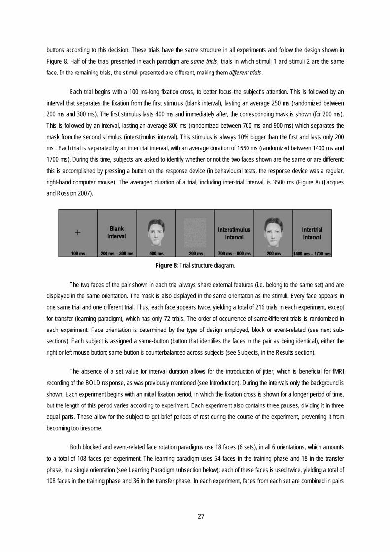
buttons according to this decision. These trials have the same structure in all experiments and follow the design shown in Figure 8. Half of the trials presented in each paradigm are same trials, trials in which stimuli 1 and stimuli 2 are the same face. In the remaining trials, the stimuli presented are different, making them different trials.

Each trial begins with a 100 ms-long fixation cross, to better focus the subject’s attention. This is followed by an interval that separates the fixation from the first stimulus (blank interval), lasting an average 250 ms (randomized between 200 ms and 300 ms). The first stimulus lasts 400 ms and immediately after, the corresponding mask is shown (for 200 ms). This is followed by an interval, lasting an average 800 ms (randomized between 700 ms and 900 ms) which separates the mask from the second stimulus (interstimulus interval). This stimulus is always 10% bigger than the first and lasts only 200 ms . Each trial is separated by an inter trial interval, with an average duration of 1550 ms (randomized between 1400 ms and 1700 ms). During this time, subjects are asked to identify whether or not the two faces shown are the same or are different: this is accomplished by pressing a button on the response device (in behavioural tests, the response device was a regular, right-hand computer mouse). The averaged duration of a trial, including inter-trial interval, is 3500 ms (Figure 8) (Jacques and Rossion 2007).

Figure 8: Trial structure diagram.

The two faces of the pair shown in each trial always share external features (i.e. belong to the same set) and are displayed in the same orientation. The mask is also displayed in the same orientation as the stimuli. Every face appears in one same trial and one different trial. Thus, each face appears twice, yielding a total of 216 trials in each experiment, except for transfer (learning paradigm), which has only 72 trials. The order of occurrence of same/different trials is randomized in each experiment. Face orientation is determined by the type of design employed, block or event-related (see next sub-sections). Each subject is assigned a same-button (button that identifies the faces in the pair as being identical), either the right or left mouse button; same-button is counterbalanced across subjects (see Subjects, in the Results section).

The absence of a set value for interval duration allows for the introduction of jitter, which is beneficial for fMRI recording of the BOLD response, as was previously mentioned (see Introduction). During the intervals only the background is shown. Each experiment begins with an initial fixation period, in which the fixation cross is shown for a longer period of time, but the length of this period varies according to experiment. Each experiment also contains three pauses, dividing it in three equal parts. These allow for the subject to get brief periods of rest during the course of the experiment, preventing it from becoming too tiresome.

Both blocked and event-related face rotation paradigms use 18 faces (6 sets), in all 6 orientations, which amounts to a total of 108 faces per experiment. The learning paradigm uses 54 faces in the training phase and 18 in the transfer phase, in a single orientation (see Learning Paradigm subsection below); each of these faces is used twice, yielding a total of 108 faces in the training phase and 36 in the transfer phase. In each experiment, faces from each set are combined in pairs

28

to determine the stimuli to be shown in each trial. Each of the paradigms used in this study will be separately analysed in the following subsections.

2.2.1. Face Rotation - Block Design Paradigm The blocked paradigm consists of 216 trials, divided into 6 blocks (according to orientation), resulting in a total of

36 blocks, each containing 6 trials. Each block corresponds to one orientation, i.e. the faces are shown in the same orientation for every trial of a given block. Each orientation occurs 6 times during the experiment, which means there are 36 trials per orientation in the whole experiment. The order of all 36 blocks (i.e. the order in which the orientations are shown) was grouped in sets of 6 in which no repetition occurred (all orientations were shown once in each set), with each set being pseudorandomized, with the aid of a script developed using MATLAB. This script was used to generate a random order matrix which was then tested to see if it respected two conditions: each pair of orientations was repeated at most twice (i.e. two orientations occurred in sequence no more than two times, so as not to generate a pattern) and successive occurrences of the same orientation were separated by at least two other orientations (i.e., the minimum distance between the same orientation is two). Additionally, 6 null blocks were added to this paradigm, as a control condition. Each of these trials lasts 21 s (average duration of a block of trials: 6 · 3.5 s = 21 s) and adds a total of 2 min 6 s to the design. The initial fixation lasts 21 s (or 27 s = 21 s + 6 s, in fMRI design, to accommodate for scanner delay) which makes the design 15 min 3 s long (15 min 9 s in fMRI); when divided in runs, each run is 5 min 15 s long (5 min 21 s in fMRI). The apparent discrepancy in run length is a consequence of run structure: each run has its own initial fixation period, so run length is slightly larger than one third of total paradigm length. The structure of the Face Rotation-Block Design paradigm is shown in Figure 9.

Figure 9: Block Design paradigm diagram. 6 consecutive blocks of stimuli are followed by a fixation block, of the same length. This pattern is repeated 6 times throughout the paradigm, with the orientation order changing each time. The

orientation order shown corresponds to the first 6 blocks.

2.2.2. Face Rotation - Event-Related Design Paradigm Similarly to block design, this experiment is also comprised of 216 trials. However, contrary to block design, trials

are not grouped together in sets of 6 according to orientation, instead occurring individually, with no relation to the previous or the consecutive trial. The occurrence of any orientation is not preset but rather pseudorandomized. 36 null trials (216:36=6, so the ratio of trials to null trials is 6:1) were also added, interspersed and randomized with the remaining trials. In these trials only the fixation cross is shown and their duration is the averaged duration of a trial (3.5 s). The initial fixation runs longer, lasting 12 s (or 18 s = 12 s + 6 s, in fMRI design, to accommodate for scanner delay). Thus, the total duration of the design is approximately 14 min 54 s (15 min in fMRI); when divided in runs, each run is 5 min 6 s (5 min 12 s in fMRI). As occurred in block design, the apparent discrepancy in run length is a consequence of each run having its own initial fixation period. The structure of the Face Rotation-Event-Related Design paradigm is shown in Figure 10.

Figure 1task trialsthe presen

2.2.3. LeT

essentiallystimuli arethe length applicablethe only ewould be aanother orin Figure 1

Figure 11for the L

other word

TrainingS

36 null triatrials throuapproxima

TransferA

is a shorte

10: Example of s: each colour idnce of jitter. Th

earning ParaThis experimeny similar in natue oriented at 12 of the paradigm to every param

experiment to bapplied on the frientation, name11.

1: Example of aLearning Paradds, the first bloc

FR-BD and F

g Phase Since this paraals were introduughout the expately 14 min 54

r Phase Although its baer run, having o

an Event-Relatdentifies a differhe ratio (task tri

adigm nt is comprisedure, they differ 20°, in the transm, the transfer meter of the pabe repeated on fourth day, afteely the complem

a parametric deigm. Each blocck contains the FR-ER, total nu

adigm deals onluced (thus presperiment and la s.

sic structure is only one third o

ted design diagrent stimuli leveals)/(fixation tri

figure in

d of two distinct in size and in sfer phase, the phase is one tharadigm, be it n each subject or the learning smentary. The st

esign diagram. Tk contains a nu first 6 trials, thember of blocks

y with one orieserving the 6:1 asting 3.5 s. Th

very similar toof the trials, 72.

29

gram. Red linesel. Notice that thals) is not the sn (Mechelli et a

t phases: the t the orientation orientation usehird of the trainnumber of stimuover a period osession, to assetructure of the F

The parameter umber of trials (e second trials is 36. For the t

entation, its 216ratio between t

he initial fixation

that of the lea It also has a s

represent fixathe distance betsame as was usl. 2003)]

raining phase a of the faces p

ed is 240° (as eing phase, whic

uli, number of tof several daysess whether it isFace Learning

in question is b6 in the case of7 to 12, and sotransfer phase,

6 trials occur intrials and null trn period lasts 1

rning experimesmaller number

tion trials; the retween each barsed in the curre

and the transfepresented: whileexplained in thech translates inrials or number

s, in this case, s possible to tra– Training + Tr

block, which is tf Learning), occ

o on. For Learni total number o

dividually and arials), occurring12 s. The total

ent (trial structur of stimuli – 18

emaining lines rr is not uniform,ent paradigm. [B

er phase. Whilee in the traininge Introduction).nto a 1:3 ratio. Tr of null trials. T 4. The transfeansfer that knowransfer paradigm

the parameter ccurring in succeng (training phaf blocks is 12.

are not groupeg interspersed w duration of the

re remains unc8 – but these ar

represent , indicating Based on a

e these are g phase all Regarding This ratio is This is also

er paradigm wledge into m is shown

considered ession. In ase), as for

d into sets: with regular e design is

changed), it re repeated

30

and each occurs twice. The number of null trials is also decreased to a third, there being only 12 and these remain interspersed. The initial fixation period is 12 s long and the design lasts approximately 5 min 6 sec.

2.2.4. FFA-PPA-LOC Localiser The FFA-PPA-LOC Localiser paradigm was largely based on Peelen and Downing, 2005. No task is performed in

this paradigm: subjects are only required to look at the pictures being shown. This paradigm consists of four runs (Peelen and Downing 2005). These runs contain 21 blocks, each 16 s long. Five blocks are fixation-only (blocks 1, 6, 11, 16 and 21); the remaining 16 blocks present gray scale pictures falling into one of 4 categories: Houses, Faces, Objects or Scrambled

objects (generated from object pictures similarly to how masks were generated in the previous sub-section). Each non-fixation block contains 16 pictures, from a total of 32 images. Since blocks occur 4 times per run, a total of 64 pictures are presented for each category (every picture is repeated). Block order was symmetrically counterbalanced within each run; run 1 and run 3 had the same block order, as had run 2 and run 4. Figure 12 shows the two versions of block order used.

Figure 12: Block order for runs 1 and 3 (above) and runs 2 and 4 (below). Note that the last 2 sets of blocks of one run are the first 2 sets of the other run. “Dummies” correspond to the initial fixation period. Fixation blocks are identified as baseline.

Each stimulus (picture) was presented for 600 ms and followed by a 400 ms inter-stimulus interval, yielding a total run duration of 5 min 36 s. An initial fixation period occurs before the first fixation block lasting 6 s; this was thought out to accommodate the delay inherent to the fMRI machine, so that scanning and paradigm may begin at the same time.

2.3. Analysing the data: Guide User Interface (GUI) To analyse the results obtained by applying the paradigms, a multistep methodology was employed. Firstly,

Presentation was programmed to generate a logfile in each experiment recording the following information for each trial:

- relation between the faces shown ("same” or “different”); - pair of faces shown (out of 108 faces for FR-ER and FR-BD, 54 for the training phase of the learning paradigm

and 18 for the transfer phase of the same paradigm); - response button pressed (1 or 2); - response times (delay between presentation of the second face stimulus and response).

31

Secondly, a MATLAB script was written to load the Presentation logfiles and extract the relevant information for the analysis of the experiments. Since there is a total of 216 trials, it would be unpractical to analyse them all simultaneously. Accordingly, trials were grouped into sets – named blocks (even for event-related and learning paradigms) – each containing 6 trials, yielding a total of 36 blocks. Trials were grouped by orientation and by occurrence for FR-BD and FR-ER experiments (each block corresponded to one and only one orientation): blocks reflect trial order in each orientation. Considering there are 6 orientations and a total of 36 blocks (as previously discussed), each orientation will contain 6 blocks. In the learning experiment, as only one orientation is used at the same time, blocks were based only on the order by which trials occurred.

Four parameters were considered in the analysis: - number of missed trials (i.e. trials with no response; represented by integers) - error rates (for valid trials, i.e. trials with response; represented by fractions); - response times for correct trials; - response times for incorrect trials. Out of all these, response times for correct answers and error rates were considered the most relevant, so only

these parameters were stored into a matrix with the following dimensions: number of subjects · (number of blocks · number of parameters considered).

This matrix is automatically exported into a Microsoft Excel (Microsoft Corporation) sheet, which can then be loaded into other programs for further processing, such as SPSS (www.spss.com). SPSS is a statistical analysis software that is able to read data from multiple sources such as excel spreadsheets. A .txt file with the same information was also stored, to allow for the construction of the corresponding charts (see below).To better enable access to all features of this methodology, an interface was built using MATLAB (Figure 13, below).

Figure 13: Guide User Interface (GUI) designed for this study. This interface is divided into three sections, one for analysis

and one for chart-building. A third section was included to show a preview of the overall results of a given analysis; currently, the results shown are for FR – ER. All the information required for the processing of data is interactively asked the user in the

course of the respective program.

32

This GUI is divided into three sections: - Analysis of Presentation logfiles; - Chart generation showing the data resulting from the analysis; - Preview of the overall results.

In the Analysis section, the user may select the experiment to be analysed by pressing the appropriate button. Each button will activate a MATLAB function relative to the experiments. Input data relevant for the analysis, such as subject’s name, number of trials or same-button used is interactively asked of the user in a sequence of input windows. The button relative to the learning paradigm will process the results for both training and transfer phase.

The Charts section allows the elaboration of charts relative to the data obtained in the analysis section. This section is divided into two subsections: one for the face rotation paradigms (blocked and event-related) and another for the learning paradigm. Each of these subsections presents two possibilities: obtaining charts for all subjects or obtaining charts for a particular subject (subjects are identified by a number corresponding to the order in which they were introduced in the analysis section). The two subsections, Face Rotation and Learning present the same basic options: both allow the user to view results for both error rates and/or response times and both enable an averaged analysis across all levels of a factor. Selecting an individual factor level to be analysed is also possible. The Preview section traces a line plot with the averaged values or error rates and response times for the selected experiment. In the case of both Face Rotation Experiments, FR–BD and FR–ER, results are plotted by orientation; for the learning paradigm, results are plotted by session.

33

3. Materials & Methods In this chapter subjects and protocols for each paradigm will be described. Both behavioural and fMRI experiments are

considered, with the chapter being divided accordingly.

3.1. Behavioural experiments These tests were used to test the adequacy of the three paradigms to the goals of the study. As the three paradigms

used different subjects, the corresponding subsection is divided by paradigms. However, protocol was similar for both FR-BD and FR-ER; as such, it is presented under a single section.

3.1.1. Protocols

Subjects 13 unpaid volunteers participated in the BD study experiment (6 males), with an average age of 23.58±2.39 years and

average 17.58±2.43 years of education. 10 unpaid volunteers were used for the ER experiment (5 males) with an average age of 22.6 ± 1.07 years and an average education of 16.6±0.97 years. 7 unpaid volunteers were used for the Learning experiment, 3 males, with the average age of 23.3±3.20 years and average 17.4±3.05 years of education. 3 subjects used the left mouse button to identify faces as “same”.

After these subjects had participated in FR experiments, a timing error was found on Presentation while running the paradigms as a single run. This was probably due to the fact that loading all the images was too resource consuming for the computer, leading to severe delays in stimuli presentation, which impaired the results. As such, more subjects were recruited and the paradigms were split in runs (where the pauses had been).

5 new subjects were selected for the BD experiment (4 males), with an average age of 37.80±21.41 years and an average education of 11.20±5.85 years. 3 subjects used the left mouse button to identify faces as “same”. 5 new subjects were also selected for the ER experiment (1male), with an average age of 39.4±20.66 years and an average education of 14.60±3.29 years.

7 unpaid volunteers participated in the Face Learning experiment (3 males), with the average age of 23.3±3.20 years and an average 17.4±3.05 years of education. None was paid. 3 subjects used the left mouse button to answer “same”.

All subjects were right handed and had normal or corrected to normal vision.

Tasks The Face Rotation paradigms developed in this Thesis and described in section 2 were applied to the subjects,

after the respective instructions were given. The subject’s responses (same/different) were given using a computer mouse, in which one button (left or right) would correspond to a “same” answer and the other to a “different” answer. Buttons were counterbalanced across subjects. Test was preformed once on each subject, at attenuated (natural) light levels. The Training Phase of the Learning paradigm was applied on each subject for 4 consecutive days, once a day, at approximately the same time every day. At the end of the fourth day, the subjects were asked to perform the Transfer phase.

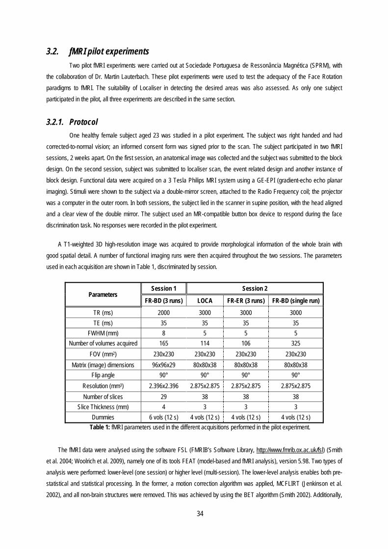
34

3.2. fMRI pilot experiments Two pilot fMRI experiments were carried out at Sociedade Portuguesa de Ressonância Magnética (SPRM), with

the collaboration of Dr. Martin Lauterbach. These pilot experiments were used to test the adequacy of the Face Rotation paradigms to fMRI. The suitability of Localiser in detecting the desired areas was also assessed. As only one subject participated in the pilot, all three experiments are described in the same section.

3.2.1. Protocol One healthy female subject aged 23 was studied in a pilot experiment. The subject was right handed and had

corrected-to-normal vision; an informed consent form was signed prior to the scan. The subject participated in two fMRI sessions, 2 weeks apart. On the first session, an anatomical image was collected and the subject was submitted to the block design. On the second session, subject was submitted to localiser scan, the event related design and another instance of block design. Functional data were acquired on a 3 Tesla Philips MRI system using a GE-EPI (gradient-echo echo planar imaging). Stimuli were shown to the subject via a double-mirror screen, attached to the Radio Frequency coil; the projector was a computer in the outer room. In both sessions, the subject lied in the scanner in supine position, with the head aligned and a clear view of the double mirror. The subject used an MR-compatible button box device to respond during the face discrimination task. No responses were recorded in the pilot experiment.

A T1-weighted 3D high-resolution image was acquired to provide morphological information of the whole brain with good spatial detail. A number of functional imaging runs were then acquired throughout the two sessions. The parameters used in each acquisition are shown in Table 1, discriminated by session.

Parameters Session 1 Session 2

FR-BD (3 runs) LOCA FR-ER (3 runs) FR-BD (single run)

TR (ms) 2000 3000 3000 3000 TE (ms) 35 35 35 35

FWHM (mm) 8 5 5 5 Number of volumes acquired 165 114 106 325

FOV (mm2) 230x230 230x230 230x230 230x230 Matrix (image) dimensions 96x96x29 80x80x38 80x80x38 80x80x38

Flip angle 90° 90° 90° 90° Resolution (mm3) 2.396x2.396 2.875x2.875 2.875x2.875 2.875x2.875 Number of slices 29 38 38 38

Slice Thickness (mm) 4 3 3 3 Dummies 6 vols (12 s) 4 vols (12 s) 4 vols (12 s) 4 vols (12 s)

Table 1: fMRI parameters used in the different acquisitions performed in the pilot experiment.

The fMRI data were analysed using the software FSL (FMRIB’s Software Library, http://www.fmrib.ox.ac.uk/fsl) (Smith et al. 2004; Woolrich et al. 2009), namely one of its tools FEAT (model-based and fMRI analysis), version 5.98. Two types of analysis were performed: lower-level (one session) or higher level (multi-session). The lower-level analysis enables both pre-statistical and statistical processing. In the former, a motion correction algorithm was applied, MCFLIRT (Jenkinson et al. 2002), and all non-brain structures were removed. This was achieved by using the BET algorithm (Smith 2002). Additionally,

35

spatial smoothing was also applied, by means of a Gaussian Kernel of FWHM = 8 mm (for FR-BD, session 1) or 5 mm (remaining acquisitions). A Gaussian-weighted least-squares straight line fitting, with sigma=50.0 s was used for temporal filtering.

In the latter, the statistical analysis per se, the analysis of the time-series was achieved using FILM with auto-correlation correction (Woolrich et al. 2001) to fit a pre-defined GLM to the data. Data were then registered to the subject’s high-resolution T1-weighted image and to the standard MNI (Montreal Neurological Institute) space (Collins et al 1995), using FLIRT (Jenkinson et al. 2002; Jenkinson and Smith 2001). Regarding the higher level analysis, it was carried out using a fixed effects model, accomplished by forcing random effects variance to 0 in FLAME, FMRIB's Local Analysis of Mixed Effects (Beckmann et al. 2003; Woolrich et al. 2004). First-level statistical maps were thresholded at p=0.005 (uncorrected) and high-level statistical maps were thresholded using clusters determined by Z>2.3 and a (corrected) cluster significance threshold of p=0.01 (Worsley 2001).

In order to build the GLM for each dataset, it is necessary to know the exact timings of the paradigm. To correctly establish them, a MATLAB script was generated. This script read the values from the logfile generated by Presentation and saved them into different variables according to its label. Each of these variables is called an explanatory variable (EV) (corresponding to in Equation 1 of the Introduction). For Face Rotation paradigms, EVs were built according to orientation (0, 60, 120, 180, 240, 300); in Localiser, EVs were based on stimulus type (Faces, Houses, Objects, Scrambled). These variables were then stored in .txt files for use in FSL. Each file contained 3 columns: one with the onset timing (relative to the start of the acquisition), one with duration of each occurrence and one with the corresponding amplitude in the design. The first temporal derivative of each EV was also added as an EV, in order to account for possible variations in the delay of the HRF, yielding a total of 13 EVs for the Face Rotation experiments and 10 EVs for the Localiser experiments.

The EVs were then combined in contrasts used for the first level analysis of the data. Statistical t tests are then performed on each contrast to assess the significance of its contribution to the model. A Z score is finally computed for each voxel, yielding a Z statistic map for each contrast. Following this step, the resulting contrasts of EVs were entered into higher level analyses (except the block design from Session 2, acquired in a single run). The statistical maps resulting from fMRI data analysis were overlaid on an MNI space template image, using Fslview (http://www.fmrib.ox.ac.uk/fsl/fslview/index.html), companion program to FSL. This program also contains an atlas tool, which allowed for the identification of the different brain areas in MNI space.

36

4. Results The results from the behavioural application of each paradigm will first be described and the results of the fMRI

pilot experiments will then be presented.

4.1. Behavioural Results Behavioural data resulting from paradigm application was subjected to pre-processing, using a MATLAB script, and

the results were saved into a .txt and .xls file. Graphics displaying the results by subject and for the group were generated, in MATLAB, and the results were loaded into SPSS for subsequent statistical analysis. A repeated measures ANOVA was performed, for both error rates and response times. The number of factors varied: both ER and blocked design had orientation and block as factors, each with 6 levels (as discussed before), while learning/transfer had one factor only, block, with 36/12 levels. In order to assess the relevance of the session in the learning process, this was introduced as a covariate.

4.1.1. Face Rotation Paradigms: Block Design The group results of Block Design, for both factors (orientation and block) and considering both variables (error

rates and response times), are summarized in Figure 14. Repeated measures ANOVA found no significant effect of block on either measure (F(0.761), p> 0.05 for error rates; F(0.570), p> 0.05 for response times). Although the effect of orientation on error rates was not significant (F(1.967), p>0.05), a significant effect was observed for response times (F(3,899), p<0.05). Further analysis demonstrated that no trend was found for either measure, whichever factor considered.

The global average reaction time was 590.83±23.3 ms and the global average error rate was 0.17±0.03. Both reaction times and error rates exhibited a quadratic pattern of variation as a function of orientation: results present an initial rise that reaches a maximum value at 120°, beginning then to decrease. This decrease does not occur in a successive manner, as orientation 5 registers higher values of response times than orientation 4. Nevertheless, orientations 4-6 (180° - 300°) all register smaller values of response times than those registered for orientation 3. Factor block elicits no discernible trend in either error rates or response times: as can be seen in these charts, this factor elicits less consistent results than orientation.

Figure 15 shows examples of individual results for each of the measures and factors considered. Analysing these results, factor block seems to lead to a less coherent effect, regardless of the variable considered: for both error rates and response times, results by block do not present a pattern, as can be seen in Figures 15a and 15b. For orientation, on the other hand, both variables present a pattern, as variable value tends to increase successively until orientation 3/4 (120°/180°), and decreasing successively afterwards (Figures 15c and 15d).

4.1.2. Face Rotation Paradigms: Event Related Design The group results of Event Related Design, for both factors (orientation and block) and considering both variables (error

rates and response times), are summarized in Figure 16. Using repeated measures ANOVA, no effect of orientation or block on either measure was found (p>>0.05). Additionally, cubic trends were found for the effect of orientation

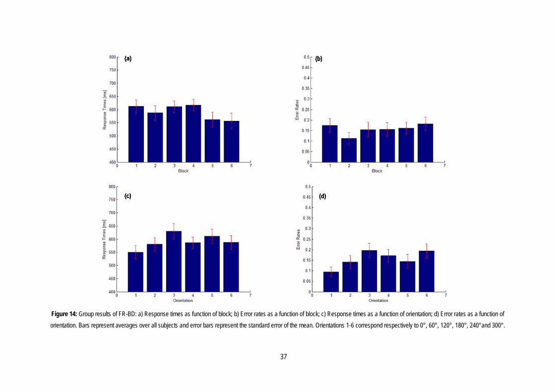
37

Figure 14: Group results of FR-BD: a) Response times as function of block; b) Error rates as a function of block; c) Response times as a function of orientation; d) Error rates as a function of orientation. Bars represent averages over all subjects and error bars represent the standard error of the mean. Orientations 1-6 correspond respectively to 0°, 60°, 120°, 180°, 240°and 300°.

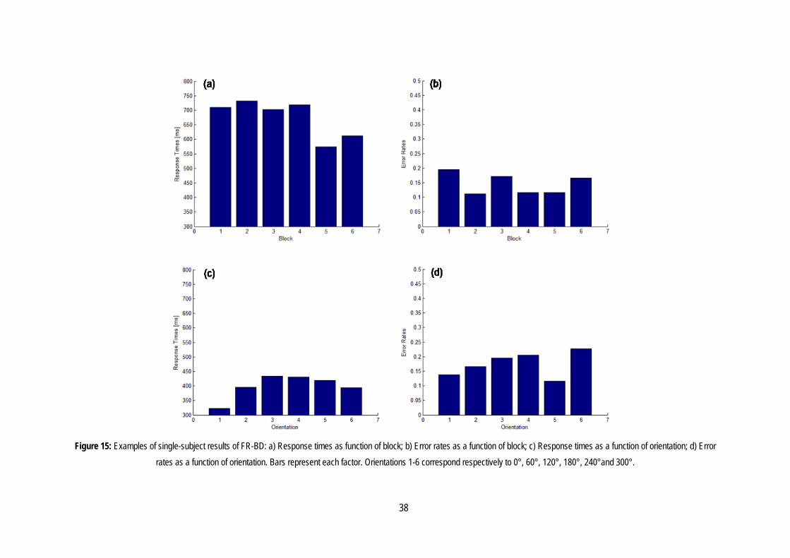
38

Figure 15: Examples of single-subject results of FR-BD: a) Response times as function of block; b) Error rates as a function of block; c) Response times as a function of orientation; d) Error

rates as a function of orientation. Bars represent each factor. Orientations 1-6 correspond respectively to 0°, 60°, 120°, 180°, 240°and 300°.

39

on response times (F(11.865), p<0.05) and the effect of block on response times (F(42.755), p<0.05). Despite the lack of statistical significance, some trends could be observed in the data. The global average reaction time was 621.13±30.04 ms and the global average error rate was 0.27±0.03. Considering error rates only, factor orientation seemed to have a more pronounced effect than factor block, as it caused a higher variability in values, which were as low as (approximately) 0.20 (block 1) and larger than 0.35 (block 4, Figure 16d). Error rates associated with block presented less variability, with value oscillating between 0.25 and 0.30, approximately (Figure 16b). Response times presented a similar behaviour, as results for factor “block” presented a higher amplitude of values, ranging from a minimum of less than 550 ms (block 1) to a maximum of over 650 ms (block 3, Figure 16a). Orientation yielded a smaller amplitude, but elicited more variability (Figure 16c). For this factor, response times register a successive increase up until the 2nd orientation (60°), but orientation 3 (120°) caused a decrease in this variable. The maximum value corresponds to orientation 4 (180°), with orientation 5 eliciting a similar, but smaller, value. The lowest value for this variable is registered for orientation 6. None of the factors shows any level of consistency, which translates in the absence of a pattern of results for both error rates and response times, with either factor.

Figure 17 shows individual results for each measure and factor analysed. In these partial results, the effects of block are still inconsistent, as neither response times nor error rates display coherent results for this factor (Figures 17a and 17b). Orientation on the other hand, displays a clear pattern for both response times and error rates (Figures 17c and 17d, respectively). In both cases, an increase in value from 0° to 180° is registered, followed by a successive decrease for orientations 5 and 6 (240° and 300°).

4.1.3. Learning Experiment The overall results of the learning experiment, as a function of session and block, are presented in Figure 18. Repeated Measures ANOVA yielded no significant effect of “Block” or “Session” (p>0.05). However, a linear trend (F(11.200), p<0.05) was found for the effect of block on error rates. For response times, the trend yielding significant results was a 4th order trend (F(4.444), p<0.46). In spite of these results, a clear trend for an effect of session on Response Times could be observed both in individual and group results. This variable seems to decrease with the effect of session, yielding a global difference (between the first and last values) of approximately 100 ms (Figure 18, left column). For error rates, the effect of session was less clear, but it is still noticeable. No clear trend was found for the effect of “block” on either response times or error rates. This is true for the two instances of learning considered: training phase (Figure 18, middle column) and transfer phase (Figure 18, right column).

Figures 19 and 20 show representative individual results for each variable analysed, respectively by block and by session. In Figure 19, block displays an erratic effect, eliciting no particular trend on any of the variables considered. This is true for both phases of the learning paradigm: training (Figures 19a and 19b) and transfer (Figures 19c and 19d). Regarding session, some of the results for individual subjects display similar trends to those registered for the group. Figure 20a demonstrates one such case, as there is a clear effect of session in response time, as was registered for the overall results. Session effect in error rates is similar to that obtained for overall results (Figure 20b).

40

Figure 16: Group results of FR-ER: a) Response times as function of block; b) Error rates as a function of block; c) Response times as a function of orientation; d) Error rates as a function of

orientation. Bars represent averages over all subjects and error bars represent the standard error of the mean. Orientations 1-6 correspond respectively to 0°, 60°, 120°, 180°, 240°and 300°.

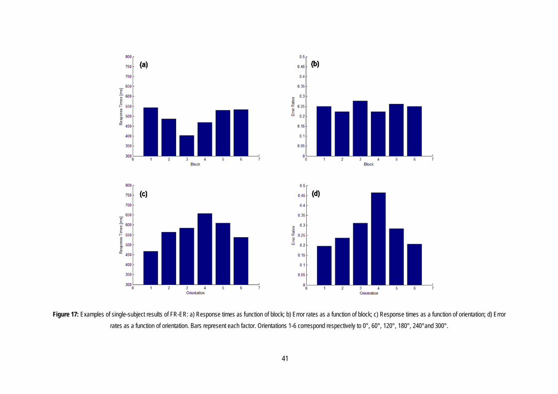
41

Figure 17: Examples of single-subject results of FR-ER: a) Response times as function of block; b) Error rates as a function of block; c) Response times as a function of orientation; d) Error rates as a function of orientation. Bars represent each factor. Orientations 1-6 correspond respectively to 0°, 60°, 120°, 180°, 240°and 300°.

42

Figure 18: Group results of the Learning experiment: error rates (top) and response times (bottom), as a function of session (left), block for training phase (middle) and block for transfer phase (right). Bars represent averages over all subjects and error bars represent the standard error of the mean. Session 5 corresponds to transfer session.

43

Figure 19: Examples of single-subject results of Learning paradigm, training phase (top) and transfer phase (bottom). Bars represent each block.

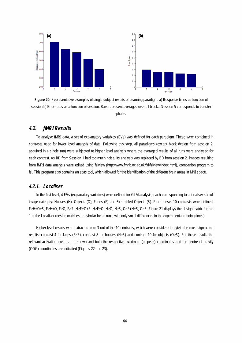
44

Figure 20: Representative examples of single-subject results of Learning paradigm: a) Response times as function of

session b) Error rates as a function of session. Bars represent averages over all blocks. Session 5 corresponds to transfer phase.

4.2. fMRI Results To analyse fMRI data, a set of explanatory variables (EVs) was defined for each paradigm. These were combined in

contrasts used for lower level analysis of data. Following this step, all paradigms (except block design from session 2, acquired in a single run) were subjected to higher level analysis where the averaged results of all runs were analysed for each contrast. As BD from Session 1 had too much noise, its analysis was replaced by BD from session 2. Images resulting from fMRI data analysis were edited using fslview (http://www.fmrib.ox.ac.uk/fsl/fslview/index.html), companion program to fsl. This program also contains an atlas tool, which allowed for the identification of the different brain areas in MNI space.

4.2.1. Localiser In the first level, 4 EVs (explanatory variables) were defined for GLM analysis, each corresponding to a localiser stimuli

image category: Houses (H), Objects (O), Faces (F) and Scrambled Objects (S). From these, 10 contrasts were defined: F>H+O+S, F>H+O, F>O, F>S, H>F+O+S, H>F+O, H>O, H>S, O>F+H+S, O>S. Figure 21 displays the design matrix for run 1 of the Localiser (design matrices are similar for all runs, with only small differences in the experimental running times).

Higher-level results were extracted from 3 out of the 10 contrasts, which were considered to yield the most significant: results: contrast 4 for faces (F>S), contrast 8 for houses (H>S) and contrast 10 for objects (O>S). For these results the relevant activation clusters are shown and both the respective maximum (or peak) coordinates and the centre of gravity (COG) coordinates are indicated (Figures 22 and 23).

45

Figure 21: Design matrix for LOCA. Time is displayed vertically and each column corresponds to an EV. Contrasts are

shown in the bottom and identified as C1-C10. The two rightmost columns pertain to the EV “Scrambled (Objects)”; the bad display is a consequence of word length.

For O>S, 10 clusters of activation were found, out of which only 2 were considered significant. These clusters are bilateral, and can be found in LOC, on the left (peak x=-42, y=-82, z=0; COG: x=-27.6, y=-42.2, z=12.6) and the right hemisphere (peak x=44, y=-72, z=-12; COG: x=39.7, y=-66.8, z=-1.28). These clusters had maximum values of Z of respectively 12.6 and 12.7 (2.3<Z<13.3).

Regarding contrast H>S, 9 clusters were found, but only two were regarded as significant. One was located in the right hemisphere (peak x=28, y= 50, z= 12; COG: x=36.3, y=-66.9, z=3.81) and the other on the left (peak x=-28, y=-52, z=-10; COG: x=-38.6; y=-69.6, z=0.0), but both pertain to the temporal occipital fusiform cortex. The right cluster registered a maximum value of Z=10.6 and for the left one Z= 9.26 (2.3<Z<11.0).

Faces (contrast F>S) also elicited 10 clusters of activation, out of which 3 were considered relevant. Contrary to what happened for houses and objects, one of these clusters displayed lateralization, occurring only in the right hemisphere (peak x= 40, y=-44, z=-24; COG: x=42.4, y=-45.5, z=-23.7), specifically in the temporal occipital fusiform cortex. For this cluster, maximum Z= 6.55. The remaining clusters are indicative of activation in LOC in both the left (peak x=-42, y=-76, z=-16; COG: x=-51.1, y=-70.2, z=-4.55) and the right hemisphere (peak x=44, y=-74, z=-8; COG: x=53.7, y=-69.2, z=1.95). Z values are Z= 6.51 for left cluster and maximum Z= 9.26 for right cluster (2.3<Z<9.3).

Figstatistical Z

(2.3<ZActiva

Fig(Red)

ure 22: ResultsZ maps are shoZ<13.3), showination for F>S (2

bilatera

gure 23: Overal, Houses (Blue)

s for Localiser, own overlaid onng the LOC bila2.3<Z<9.3), sholly); (D) Activati

l results for Loc) and Objects (G

coordinat

displayed in con the MNI tempaterally. (B) Actiowing the LOC,ion for F>S, (2.

caliser, displayeGreen) are ovees of slices are

46

oronal (left) and late image (righvation map for predominantly3<Z<9.3), show

ed in coronal (leerlaid on the MNe: y=-74 (corona

transversal (right hemisphere i H>S (2.3<Z<11

y on the right hewing the FFA, o

eft) and transveNI template andal) and z=-6 (tra

ght) planes. Thes on the left). (A1.0), showing th

emisphere (activon the right hem

ersal (right) pland right hemispheansversal).

e relevant clustA) Activation mhe PPA bilateravation was regis

misphere.

nes. Contrasts fere is on the lef

ters of the ap for O>S

ally. (C) stered

for Faces ft.. MNI

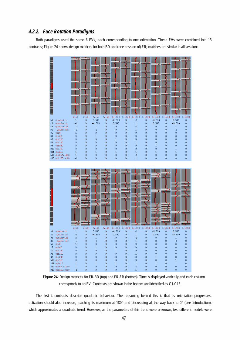
47

4.2.2. Face Rotation Paradigms Both paradigms used the same 6 EVs, each corresponding to one orientation. These EVs were combined into 13

contrasts; Figure 24 shows design matrices for both BD and (one session of) ER; matrices are similar in all sessions.

Figure 24: Design matrices for FR-BD (top) and FR-ER (bottom). Time is displayed vertically and each column

corresponds to an EV. Contrasts are shown in the bottom and identified as C1-C13.

The first 4 contrasts describe quadratic behaviour. The reasoning behind this is that as orientation progresses, activation should also increase, reaching its maximum at 180° and decreasing all the way back to 0° (see Introduction), which approximates a quadratic trend. However, as the parameters of this trend were unknown, two different models were

consideredcontrasts upright>inv

Pre-pshown in t(single runcontrast wresults for

Fdisplac

4.2.2.1. FThe r

in Figure 2x=44.4, y=and left (x3.87 and Z

d, contrast 1 a2 and 4, respverted and inve

processing of tthe motion paran) and FR-ER awas contrast 3 contrast F>S w

Figure 25: Moticements (bottom

displacemen

Face Rotatioresults obtained26. On the 6 c=-75.4, z=-5.65)x=-44, y=-46, zZ= 4.93 (3.5<Z<

and contrast 3pectively. The erted>upright.

he FR-BD expameters in Figuare displayed i(identified in F

were overlaid on

on charts for Bm) are shown font was 0.14 mm

on – Block Dd by a first-leveclusters identifie), with maximum=-22) temporal<8.9).

3. Additionally, remaining con

periment in sesure 25. This datn Figures 26 a

Figure 24 as Qn to the FR resu

D, session 1. Eor all volumes c Charts obtaine

Design l analysis of the

ed by contrast m Z=.8.86; left l occipital fusifo

48

their symmetrtrasts pertain

ssion 1 revealetaset was thereand 27, respectQuadratic1); as ults, to better id

Estimated valuecollected. Absoled from FSL pre

e Block Design 3, the followingLOC.(peak coo

orm cortex (inc

ric counterpartsto individual o

ed excessive mefore not suitabltively. For both such, only resdentify areas wh

s for rotations (ute mean disple-stats (Jenkins

experiment sing regions were ordinates x=-46cluding FFA), w

s were also inorientations, all

motion throughle for further an FR-BD and F

sults for this cohere overlappin

(top), translationacement was 1son et al. 2002;

ngle run collecte identified: righ

6, y=-78, z=-6); with maximum Z

cluded in the orientations v

out the acquisnalysis. ResultsR-ER the mostontrast are shong occurred.

ns (middle) and.95 mm; relativ Smith 2002).

ed in session 2ht LOC (peak c right (x=48, y=Z values, respe

design, as vs. fixation,

sition, as is s for FR-BD t significant own. LOCA

d mean ve mean

are shown oordinates:

=-50, z=-22) ectively, Z=

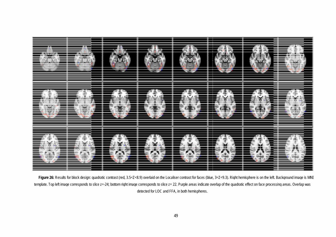
Figure 26: Restemplate. Top left i

ults for block design: mage corresponds to

quadratic contrast (reo slice z=-24; bottom r

ed, 3.5<Z<8.9) overlaright image correspon

detected fo

49

aid on the Localiser conds to slice z= 22. Puor LOC and FFA, in b

ontrast for faces (bluerple areas indicate ov

both hemispheres.

e, 3<Z<9.3). Right hemverlap of the quadratic

misphere is on the leftc effect on face proce

t. Background image essing areas. Overlap

is MNI was

Figure 27: Resuis MNI temp

.

lts for event related dplate. Top left image c

esign: quadratic contcorresponds to slice z=

rast (red, 2.3<Z<5.3) =-24; bottom right ima

50

overlaid on the Localage corresponds to sl

liser contrast for faceslice z= 22. Purple are

s (blue, 3.0<Z<9.3). Reas indicate overlap of

Right hemisphere is of results. Overlap was

n the left. Backgrounds detected for LOC.

d image

51

4.2.2.2. Face Rotation - Event Related Some runs of the FR-ER presented an artifact known as Gibbs Ringing. This effect polluted the results and hindered a

proper higher-level analysis. As the first run was unaffected by this artifact, its results were usable, and are thus the results shown in Figure 27 (previous page). An example of Gibbs Ringing is included in figure 28.

Figure 28: Example of Gibbs ringing obtained for run 2 of FR-ER.

The contrast used yielded 7 clusters of activation, including the following areas: left LOC (peak coordinates 52.9,-65.1, 21), with maximum Z= 4.16; right LOC (peak coordinates x=-57.8, y=-69.4, z=8.24), with maximum Z= 5.17; right inferior temporal gyrus, temporo-occipital part (peak coordinates x=48, y=-56, z=-16), with maximum Z= 2.67 (2.3<Z<5.3). No similar activation was found in the left hemisphere.

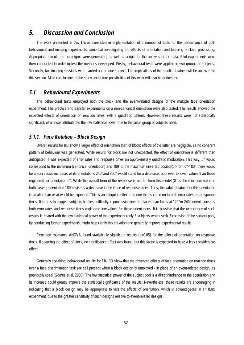
52

5. Discussion and Conclusion The work presented in this Thesis consisted in implementation of a number of tools for the performance of both

behavioural and imaging experiments, aimed at investigating the effects of orientation and learning on face processing. Appropriate stimuli and paradigms were generated, as well as scripts for the analysis of the data. Pilot experiments were then conducted in order to test the methods developed. Firstly, behavioural tests were applied in two groups of subjects. Secondly, two imaging sessions were carried out on one subject. The implications of the results obtained will be analyzed in this section. Main conclusions of the study and future possibilities of this work will also be addressed.

5.1. Behavioural Experiments The behavioural tests employed both the block and the event-related designs of the multiple face orientation

experiment. The practice and transfer experiments on a non-canonical orientation were also tested. The results showed the expected effects of orientation on reaction times, with a quadratic pattern. However, these results were not statistically significant, which was attributed to the low statistical power due to the small group of subjects used.

5.1.1. Face Rotation – Block Design Overall results for BD show a larger effect of orientation than of block: effects of the latter are negligible, as no coherent

pattern of behaviour was generated. While results for block are not unexpected, the effect of orientation is different than anticipated: it was expected of error rates and response times an approximately quadratic modulation. This way, 0° would correspond to the minimum (canonical orientation) and 180°to the maximum (inverted position). From 0°-180° there would be a successive increase, while orientations 240°and 300° would stand for a decrease, but never to lower values than those registered for orientation 0°. While the overall form of the response is not far from this model (0° is the minimum value in both cases), orientation 180°registers a decrease in the value of response times. Thus, the value obtained for this orientation is smaller than what would be expected. This is an intriguing effect and one that is common to both error rates and response times. It seems to suggest subjects had less difficulty in processing inverted faces than faces at 120°or 240° orientations, as both error rates and response times registered low values for these orientations. It is possible that the occurrence of such results is related with the low statistical power of the experiment (only 5 subjects were used). Expansion of the subject pool, by conducting further experiments, might help clarify this situation and generally improve experimental results.

Repeated measures ANOVA found statistically significant results (p<0.05) for the effect of orientation on response times. Regarding the effect of block, no significance effect was found, but this factor is expected to have a less considerable effect.

Generally speaking, behavioural results for FR- BD show that the observed effects of face orientation on reaction times over a face discrimination task are still present when a block design is employed - in place of an event-related design, as previously used (Gomes et al. 2009). The low statistical power of the subject pool is a direct hindrance to the acquisition and its increase could greatly improve the statistical significance of the results. Nevertheless, these results are encouraging in indicating that a block design may be appropriate to test the effects of orientation, which is advantageous in an fMRI experiment, due to the greater sensitivity of such designs relative to event-related designs.

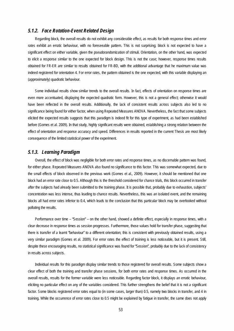
53

5.1.2. Face Rotation-Event Related Design Regarding block, the overall results do not exhibit any considerable effect, as results for both response times and error

rates exhibit an erratic behaviour, with no foreseeable pattern. This is not surprising; block is not expected to have a significant effect on either variable, given the pseudorandomization of stimuli. Orientation, on the other hand, was expected to elicit a response similar to the one expected for block design. This is not the case; however, response times results obtained for FR-ER are similar to results obtained for FR-BD, with the additional advantage that he maximum value was indeed registered for orientation 4. For error rates, the pattern obtained is the one expected, with this variable displaying an (approximately) quadratic behaviour.

Some individual results show similar trends to the overall results. In fact, effects of orientation on response times are even more accentuated, displaying the expected quadratic form. However, this is not a general effect; otherwise it would have been reflected in the overall results. Additionally, the lack of consistent results across subjects also led to no significance being found for either factor, when using Repeated Measures ANOVA. Nevertheless, the fact that some subjects elicited the expected results suggests that this paradigm is indeed fit for this type of experiment, as had been established before (Gomes et al. 2009). In that study, highly significant results were obtained, establishing a strong relation between the effect of orientation and response accuracy and speed. Differences in results reported in the current Thesis are most likely consequence of the limited statistical power of the experiment.

5.1.3. Learning Paradigm Overall, the effect of block was negligible for both error rates and response times, as no discernable pattern was found,

for either phase. Repeated Measures ANOVA also found no significance to this factor. This was somewhat expected, due to the small effects of block observed in the previous work (Gomes et al., 2009). However, it should be mentioned that one block had an error rate close to 0.5. Although this is the threshold considered for chance trials, this block occurred in transfer after the subjects had already been submitted to the training phase. It is possible that, probably due to exhaustion, subjects’ concentration was less intense, thus leading to chance results. Nevertheless, this was an isolated event, and the remaining blocks all had error rates inferior to 0.4, which leads to the conclusion that this particular block may be overlooked without polluting the results.

Performance over time – “Session” – on the other hand, showed a definite effect, especially in response times, with a clear decrease in response times as session progresses. Furthermore, those values hold for transfer phase, suggesting that there is transfer of a learnt “behaviour” to a different orientation; this is consistent with previously obtained results, using a very similar paradigm (Gomes et al. 2009). For error rates the effect of training is less noticeable, but it is present. Still, despite these encouraging results, no statistical significance was found for “Session”, probably due to the lack of consistency in results across subjects.

Individual results for this paradigm display similar trends to those registered for overall results. Some subjects show a clear effect of both the training and transfer phase sessions, for both error rates and response times. As occurred in the overall results, results for the former variable were less noticeable. Regarding factor block, it displays an erratic behaviour, eliciting no particular effect on any of the variables considered. This further strengthens the belief that it is not a significant factor. Some blocks registered error rates equal to (in some cases, larger than) 0.5, namely two blocks in transfer, and 4 in training. While the occurrence of error rates close to 0.5 might be explained by fatigue in transfer, the same does not apply

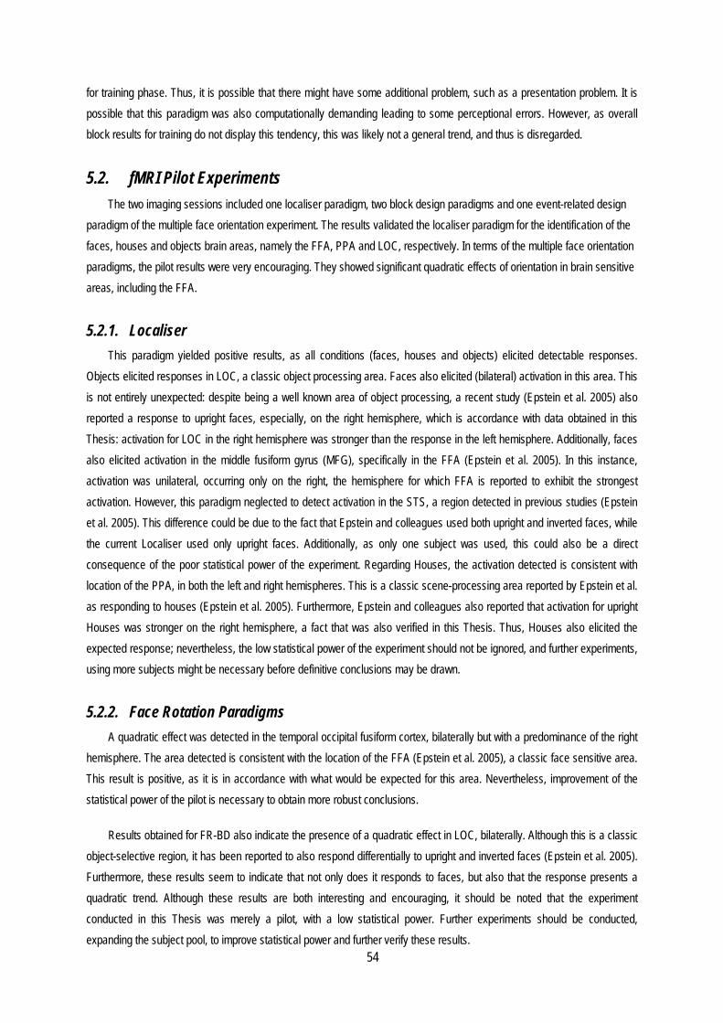
54

for training phase. Thus, it is possible that there might have some additional problem, such as a presentation problem. It is possible that this paradigm was also computationally demanding leading to some perceptional errors. However, as overall block results for training do not display this tendency, this was likely not a general trend, and thus is disregarded.

5.2. fMRI Pilot Experiments The two imaging sessions included one localiser paradigm, two block design paradigms and one event-related design

paradigm of the multiple face orientation experiment. The results validated the localiser paradigm for the identification of the faces, houses and objects brain areas, namely the FFA, PPA and LOC, respectively. In terms of the multiple face orientation paradigms, the pilot results were very encouraging. They showed significant quadratic effects of orientation in brain sensitive areas, including the FFA.

5.2.1. Localiser This paradigm yielded positive results, as all conditions (faces, houses and objects) elicited detectable responses.

Objects elicited responses in LOC, a classic object processing area. Faces also elicited (bilateral) activation in this area. This is not entirely unexpected: despite being a well known area of object processing, a recent study (Epstein et al. 2005) also reported a response to upright faces, especially, on the right hemisphere, which is accordance with data obtained in this Thesis: activation for LOC in the right hemisphere was stronger than the response in the left hemisphere. Additionally, faces also elicited activation in the middle fusiform gyrus (MFG), specifically in the FFA (Epstein et al. 2005). In this instance, activation was unilateral, occurring only on the right, the hemisphere for which FFA is reported to exhibit the strongest activation. However, this paradigm neglected to detect activation in the STS, a region detected in previous studies (Epstein et al. 2005). This difference could be due to the fact that Epstein and colleagues used both upright and inverted faces, while the current Localiser used only upright faces. Additionally, as only one subject was used, this could also be a direct consequence of the poor statistical power of the experiment. Regarding Houses, the activation detected is consistent with location of the PPA, in both the left and right hemispheres. This is a classic scene-processing area reported by Epstein et al. as responding to houses (Epstein et al. 2005). Furthermore, Epstein and colleagues also reported that activation for upright Houses was stronger on the right hemisphere, a fact that was also verified in this Thesis. Thus, Houses also elicited the expected response; nevertheless, the low statistical power of the experiment should not be ignored, and further experiments, using more subjects might be necessary before definitive conclusions may be drawn.

5.2.2. Face Rotation Paradigms A quadratic effect was detected in the temporal occipital fusiform cortex, bilaterally but with a predominance of the right

hemisphere. The area detected is consistent with the location of the FFA (Epstein et al. 2005), a classic face sensitive area. This result is positive, as it is in accordance with what would be expected for this area. Nevertheless, improvement of the statistical power of the pilot is necessary to obtain more robust conclusions.

Results obtained for FR-BD also indicate the presence of a quadratic effect in LOC, bilaterally. Although this is a classic object-selective region, it has been reported to also respond differentially to upright and inverted faces (Epstein et al. 2005). Furthermore, these results seem to indicate that not only does it responds to faces, but also that the response presents a quadratic trend. Although these results are both interesting and encouraging, it should be noted that the experiment conducted in this Thesis was merely a pilot, with a low statistical power. Further experiments should be conducted, expanding the subject pool, to improve statistical power and further verify these results.

55

When comparing the results obtained for FR-BD with the results obtained with LOCA (for faces), an overlap of activations is detected. The areas identified by Localiser as being faces areas do indeed register a quadratic modulation of activation in the presence of faces at multiple orientations. This is an interesting result, as it verifies the validity of the results obtained for LOCA, despite the low statistical power of both experiments.

The results obtained for FR-ER pertain only to one run, due to the problems stated above (see Results section). As such, besides being affected by the low statistical power of the pilot, results shown correspond to only 1/3 of the total experiment, thus making them even less robust. Nevertheless, this paradigm yielded significant results: quadratic effects were detected for bilaterally for LOC, as had occurred for FR-BD, which supports the claim that in the presence of faces in multiple orientations, activation in this area does follow a quadratic modulation. Quadratic effects were also detected in a location consistent with the FFA, as would be expected. Naturally, new experiments are necessary to allow for more robust and general conclusions. This entails not only an increasing statistical power but also overcoming the effects of the artifact detected.

Comparing the results obtained for FR-ER with the face areas identified by Localiser, an overlap was detected bilaterally for LOC, but no overlap was detected for FFA. While results for LOC further validate LOCA, the lack of overlapping activation in the area identified as the FFA seems to suggest that there is some incompatibility between the experiments. Although there was no overlap, both paradigms, individually, elicited activation in areas consistent with FFA. In light of the additional limitations of FR-ER (only 1/3 of the results were used), these results can be considered inconclusive, since it is not possible to draw definitive conclusions from this data.

Generally speaking, results obtained for both FR paradigms, despite all the limitations of the experiments conducted, detected activation in primary visual areas. Although this is not the most significant result to be extracted from this Thesis, it is, undoubtedly, an important result, as it is in accordance with the theory that FIE occurs during face perception and not during its processing.

5.3. Conclusions and Future Directions Despite lacking in statistical power, all the paradigms were able to yield at least partially expected designs. In Learning,

for instance, there was no statistically significant effect of session, although there was an overall decrease in response times. Regarding Face Rotation paradigms, their performance in overall tests is considered equivalent. However, in the fMRI pilot, FR-BD detected quadratic activation in more areas associated with face processing. Furthermore, results for this paradigm were in accordance with LOCA results, as overlapping with these results was achieved for identified areas. FR-ER on the other hand, only achieved results consistent with LOCA for 2 of the 3 identified areas. However, these results were analysed using only one third of the experiment (one run), which attests for their robustness. Nevertheless, the current data does not support any definitive conclusions, and results comparing the efficiency of both paradigms in this kind of study are inconclusive. Localiser also failed to elicit activation in STS, a well established face area, although expected scene- object- and (other) face-specific areas were correctly detected by this paradigm.

It is important to stress that all of the behavioural tests displayed poor statistical power, consequence of a limited pool of subjects. Further tests, using more subjects could greatly improve the performance of the paradigms. However, this is not the only point in which there can be improvement. Future developments may also include paradigm optimization or stimuli redesigning. Pre and post-processing scripts could also be improved, and, perhaps be made more effective and generalist.

56

Application of ROI analysis, besides the whole-brain analysis performed here, for the assessment of face orientation effects is also an interesting future development, as it might help to investigate changes in brain activity in pre-defined brain areas, with improved sensitivity.

57

6. References Amaro, E., and Barker, G. J. (2006). "Study Design in fMRI: Basic Principles." Brain and Cognition(60), 220 - 232.

Beckmann, C., Jenkinson, M., and Smith, S. M. (2003). "General multi-level linear modelling for group analysis in FMRI."

NeuroImage(20), 1052-1063.

Büchel, C., Holmes, A. P., Rees, G., and Friston, K. J. (1998). "Characterizing Stimulus-Response Functions Using

Nonlinear Regressors in Parametric fMRI Experiments." Neuroimage( 8), 140-148.

Collins et al. (1995). "Automatic 3-D model-based neuroanatomical segmentation." Human Brain Mapping, 3(3), 190-208.

Epstein, R. A., Higgins, J. S., Parker, W., Aguirre, G. K., and Cooperman, S. (2005). "Cortical correlates of face and scene

inversion: A comparison." NeuroPsychologia(44), 1145-1158.

Friston, K. J. (2005). "Models of Brain Function in Neuroimaging." Annu. Rev. Psychol. (56), 57-87.

Gauthier, I., Williams, P., Tarr, M. J., and Tanaka, J. (1998). "Training 'greeble' experts: a framework for studying expert

object recognition processes." Vision Research(38), 2401-2428.

Gomes, C. A., Mendes, M., and Figueiredo, P. (2009). "Perceptual learning for multiple face orientations." Perception, ECVP

Abstract Supplement(38), 79.

Grill-Spector, K., and Malach, R. (2004). "The Human Visual Cortex." Annu. Rev. Neurosci.(27), 649-677.

Huettel, S. A., Song, A. W., and MacCarthy, G. (2004). Functional Magnetic Resonance Imaging, Sinauer, Sunderland,

Massachusets U.S.A.

Jacques, C., and Rossion, B. (2007). "Early electrophisiological responses to multiple face orientations correlate with

individual discrimination performances in humans." NeuroImage( 36), 863-876.

Jenkinson, M., Bannister, P., Brady, M., and Smith, S. (2002). "Improved Optimisation for the Robust and Accurate Linear

Registration and Motion Correction of Brain Images." NeuroImage, 17(2), 825-841.

Jenkinson, M., and Smith, S. M. (2001). "A Global Optimisation Method for Robust Affine Registration of Brain Images."

Medical Image Analysis, 5(2), 143-156.

Kanwisher, N., and Yovel, G. (2006). "The fusiform face area: a cortical region specialized for the perception of faces." Phil.

Trans. R. Soc. B(361), 2109-2128.

Logothetis, N. K., and Wandell, B. A. (2004). "Interpreting the BOLD signal." Annu. Rev. Physiol.(63), 735-769.

Mechelli, A., Price, C. J., Henson, R. N. A., and Friston, K. J. (2003). "Estimating Efficiency a priori: a comparison of blocked

and randomized designs." NeuroImage(18), 798-805.

Ogawa, S., Lee, T. M., Kay, A. R., and Tank, D. W. (1990). "Brain magnetic resonance imaging with contrast dependent on

blood oxygenation." Proc. Natl. Acad. Sci., 87, 9868 - 9872.

58

Peelen, M. V., and Downing, P. E. (2005). "Within-Subject Reproducibility of Category-Specific Visual Activation With

Functional MRI." Human Brain Mapping(25), 402-408.

Rossion, B. (2008). "Picture-plane inversion leads to qualitative changes of face perception." Acta Psychologica(128), 274-

289.

Rossion, B., and Gauthier, I. (2002). "How does the brain process upright and inverted faces?" Behavioral and Cognitive

Neuroscience Reviews, 1(1), 62-74.

Schiltz, C., and Rossion, B. (2006). "Faces are represented holistically in the human occipito-temporal cortex."

NeuroImage(32), 1385-1394.

Smith, S. (2002). "Fast Robust Automated Brain Extraction." Human Brain Mapping, 17(3), 143-155

Smith, S. M., Jenkinson, M., Woolrich, M. W., Beckmann, C. F., Behrens, T. E. J., Johansen-Berg, H., Bannister, P. R., Luca,

M. D., Drobnjak, I., Flitney, D. E., Niazy, R., Saunders, J., Vickers, J., Zhang, Y., Stefano, N. D., Brady, J. M., and

Matthews., P. M. (2004). " Advances in functional and structural MR image analysis and implementation as FSL."

NeuroImage, 23(S1), 208-219.

Webb, A. (2003). Introduction to Biomedical Imaging, John Wiley & Sons, Inc., Hoboken, New Jersey.

Woolrich, M. W., Behrens, T. E. J., and Beckmann, C. F. (2004). "Multi-level linear modelling for FMRI group analysis using

Bayesian inference." NeuroImage, 21(4), 1732-1747.

Woolrich, M. W., Jbabdi, S., Patenaude, B., Chappell, M., Makni, S., Behrens, T., Beckmann, C., Jenkinson, M., and Smith,

S. M. (2009). "Bayesian analysis of neuroimaging data in FSL." NeuroImage, 45(S), 173-186.

Woolrich, M. W., Ripley, B. D., Brady, J. M., and Smith, S. M. (2001). "Temporal Autocorrelation in Univariate Linear

Modelling of FMRI Data." NeuroImage, 14(6), 1370-1386.

Worsley, K. J. (2001). "Statistical analysis of activation images." Ch 14, in Functional MRI: An Introduction to Methods, P.

Jezzard, P. M. Matthews, and S. M. Smith., eds., Oxford University Press.

Yovel, G., and Kanwisher, N. (2005). "The Neural Basis of the Face-Inversion Effect." Current Biology( 15), 2256-2262.

Zwaigenbaum, L., Bryson, S., Rogers, T., Roberts, W., Brian, J., and Szatmari, P. (2005). "Behavioral manifestations of

autism in the first year of life." Int. J. Devl Neuroscience( 23), 143–152.